Probing inner and outer disk misalignments in transition disks

A. J. Bohn; M. Benisty; K. Perraut; N. van der Marel; L. Wölfer; E. F. van Dishoeck; S. Facchini; C. F. Manara; R. Teague; L. Francis; J.-P. Berger; R. Garcia-Lopez; C. Ginski; T. Henning; M. Kenworthy; S. Kraus; F. Ménard; A. Mérand; L. M. Pérez

doi:10.1051/0004-6361/202142070

Home

All issues

Volume 658 (February 2022)

A&A, 658 (2022) A183

Full HTML

Open Access

Issue		A&A Volume 658, February 2022


Article Number		A183
Number of page(s)		30
Section		Interstellar and circumstellar matter
DOI		https://doi.org/10.1051/0004-6361/202142070
Published online		22 February 2022

A&A 658, A183 (2022)

Constraints from VLTI/GRAVITY and ALMA observations^★

A. J. Bohn¹^,2, M. Benisty³^,2, K. Perraut², N. van der Marel⁴^,1^,★, L. Wölfer⁵^,9, E. F. van Dishoeck¹^,5, S. Facchini⁶^,7, C. F. Manara⁷, R. Teague⁸, L. Francis⁴, J.-P. Berger², R. Garcia-Lopez¹⁰^,11, C. Ginski¹, T. Henning¹¹, M. Kenworthy¹, S. Kraus¹², F. Ménard², A. Mérand⁷ and L. M. Pérez¹³

¹ Leiden Observatory, Leiden University, PO Box 9513, 2300 RA Leiden, The Netherlands
e-mail: ajbohn.astro@gmail.com
² Univ. Grenoble Alpes, CNRS, IPAG, 38000 Grenoble, France
³ Unidad Mixta Internacional Franco-Chilena de Astronomía (CNRS, UMI 3386), Departamento de Astronomía, Universidad de Chile, Camino El Observatorio 1515, Las Condes, Santiago, Chile
e-mail: Myriam.Benisty@univ-grenoble-alpes.fr
⁴ Physics & Astronomy Department, University of Victoria, 3800 Finnerty Road, Victoria, BC, V8P 5C2, Canada
⁵ Max-Planck Institut für Extraterrestrische Physik (MPE), Gießenbachstraße 1, 85748 Garching, Germany
⁶ Università degli Studi di Milano, via Giovanni Celoria 16, 20133 Milano, Italy
⁷ European Southern Observatory, Karl-Schwarzschild-Str. 2, 85748 Garching, Germany
⁸ Center for Astrophysics | Harvard & Smithsonian, 60 Garden Street, Cambridge, MA 02138, USA
⁹ Universitäts-Sternwarte München, Scheinerstr. 1, 81679 München, Germany
¹⁰ School of Physics, University College Dublin, Belfield, Dublin 4, Ireland
¹¹ Max Planck Institute for Astronomy, Königstuhl 17, 69117, Heidelberg, Germany
¹² University of Exeter, School of Physics & Astronomy, Exeter, EX4 4QL, UK
¹³ Departamento de Astronomía, Universidad de Chile, Camino El Observatorio 1515, Las Condes, Santiago, Chile

Received: 23 August 2021
Accepted: 25 November 2021

Abstract

Context. Transition disks are protoplanetary disks with dust-depleted cavities, possibly indicating substantial clearing of their dust content by a massive companion. For several known transition disks, dark regions interpreted as shadows have been observed in scattered light imaging and are hypothesized to originate from misalignments between distinct regions of the disk.

Aims. We aim to investigate the presence of misalignments in transition disks. We study the inner disk (<1 au) geometries of a sample of 20 well-known transition disks with Very Large Telescope Interferometer (VLTI) GRAVITY observations and use complementary ¹²CO and ¹³CO molecular line archival data from the Atacama Large Millimeter/submillimeter Array (ALMA) to derive the orientation of the outer disk regions (>10 au).

Methods. We fit simple parametric models to the visibilities and closure phases of the GRAVITY data to derive the inclination and position angle of the inner disks. The outer disk geometries were derived from Keplerian fits to the ALMA velocity maps and compared to the inner disk constraints. We also predicted the locations of expected shadows for significantly misaligned systems.

Results. Our analysis reveals six disks to exhibit significant misalignments between their inner and outer disk structures. The predicted shadow positions agree well with the scattered light images of HD 100453 and HD 142527, and we find supporting evidence for a shadow in the south of the disk around CQ Tau. In the other three targets for which we infer significantly misaligned disks, V1247 Ori, V1366 Ori, and RY Lup, we do not see any evident sign of shadows in the scattered light images. The scattered light shadows observed in DoAr 44, HD 135344 B, and HD 139614 are consistent with our observations, yet the underlying morphology is likely too complex to be described properly by our models and the accuracy achieved by our observations.

Conclusions. The combination of near infrared and submillimeter interferometric observations allows us to assess the geometries of the innermost disk regions and those of the outer disk. Whereas we can derive precise constraints on the potential shadow positions for well-resolved inner disks around Herbig Ae/Be stars, the large statistical uncertainties for the marginally resolved inner disks around the T Tauri stars of our sample make it difficult to extract conclusive constraints for the presence of shadows in these systems.

Key words: protoplanetary disks

^★

Based on observations collected at the European Organisation for Astronomical Research in the Southern Hemisphere under ESO programs 098.D-0488(A), 099.B-0162(F), 099.C-0667(B), 0100.C-0278(E), 0101.C-0311(B), 0101.C-0281(A,B), 0102.C-0210(A), 0102.C-0408(A,D), 0103.C-0097(A), 0103.C-0347(C), 0104.C-0567(A,C), and 106.21JR.001. ALMA Program IDs are provided in the acknowledgments. All codes used for the data analysis, as well as example data files, are available at https://github.com/18alex96/disk_misalignments

^★

Banting Research fellow.

© A. J. Bohn et al. 2022

Open Access article, published by EDP Sciences, under the terms of the Creative Commons Attribution License (https://creativecommons.org/licenses/by/4.0), which permits unrestricted use, distribution, and reproduction in any medium, provided the original work is properly cited.

1 Introduction

Studying protoplanetary disks around pre-main sequence stars allows us to constrain the early stages of planet formation. Observations with the Atacama Large Millimiter/submillimeter Array (ALMA; ALMA Partnership 2015) have provided unprecedented insights in the large-scale dust and gas distributions in protoplanetary disks (e.g., van der Marel et al. 2013; Pérez et al. 2014; Andrews et al. 2018; van Terwisga et al. 2019; Teague et al. 2019). Adaptive-optics-assisted high-contrast imagers, such as the Spectro-Polarimetric High-contrast Exoplanet REsearch (SPHERE; Beuzit et al. 2019) instrument, have provided complementary scattered-light images, revealing the 3D geometries of these disks (e.g., Monnier et al. 2017; Uyama et al. 2020a). In both wavelength regimes, observations demonstrated that substructures such as rings, gaps, and spiral arms are ubiquitous in these disks (Garufi et al. 2018; Andrews 2020) and they might be linked to recently formed giant planets (Bae et al. 2017; Huang et al. 2018).

While the outer disk regions can be probed with these techniques, the innermost disk regions at scales below 1 au remain unresolved. However, the processes that are shaping these inner regions are of great interest, as they might play an important role for the formation and evolution of terrestrial planets. At such distances from the star, dust grains sublimate (at T ~ 1300–1500 K; Kama et al. 2009)and the dust sublimation front (rim) is thought to be directly irradiated by the central star, and as a consequence, to puff up and predominantly emit in the near-infrared regime (e.g., Natta et al. 2001; Isella & Natta 2005; Dullemond & Monnier 2010). Models of the rim indicate that it is a radially extended region, rather than a sharp edge, with its exact morphology depending on the properties and composition of the dust grains (Kama et al. 2009). Observationally, the innermost disk regions can be studied with infrared interferometry, which enables milli-arcsecond (subau) resolution. Early observations of Herbig AeBe stars indicated a correlation between the inner disk radii and the stellar luminosity, supporting the presence of a rim at the dust sublimation radius (Monnier et al. 2005). Subsequent studies of specific objects (e.g., Tannirkulam et al. 2008; Benisty et al. 2010; Setterholm et al. 2018; Davies et al. 2020; GRAVITY Collaboration 2020), or snapshot observations of large disk samples (Menu et al. 2015; Lazareff et al. 2017; GRAVITY Collaboration 2019), enabled us to get more insights on the rim morphology. Detailed analysis of individual disks can now be achieved over a broader wavelength regime by combining all Very Large Telescope Interferometer (VLTI) instruments (e.g., GRAVITY, MATISSE; GRAVITY Collaboration 2021; Varga et al. 2021).

In this paper, we focus on connecting the geometry of the inner disk with that of the outer disk in a subclass of protoplanetary disks, the transition disks. Transition disks were originally identified through their spectral energy distributions (SEDs) that show a characteristic absence of excess infrared emission (e.g., Strom et al. 1989; Skrutskie et al. 1990; Calvet et al. 2002). Such a dip in the SEDs indicates that the inner regions are (partially) cleared of dust material (Espaillat et al. 2014), with a cavity possibly due to the dynamical clearing by massive companions or planets (e.g., Zhu et al. 2011; Bae et al. 2019). These cavities can either be probed by (sub)millimeter interferometric imaging in both dust and gas tracers (e.g., van der Marel et al. 2016, 2018; Dong et al. 2017), mid-infrared interferometry (e.g., Kraus et al. 2013; Kluska et al. 2018; Menu et al. 2014), or in scattered light images (e.g., Bohn et al. 2019; de Boer et al. 2020). Several transition disk scattered light images present dark regions (e.g., Stolker et al. 2016; Casassus et al. 2018), which are interpreted as shadows resulting from a misalignment between inner and outer disk regions (e.g., Marino et al. 2015; Facchini et al. 2018; Nealon et al. 2019). Depending on the misalignment angle, the shadows can appear as narrow lines (Benisty et al. 2017), or as very broad areas (Benisty et al. 2018; Muro-Arena et al. 2020). Such a misalignment between disk regions might not be uncommon, and could be induced by various mechanisms detailed in the discussion section. In this paper, we search for evidence of misalignments in a sample of 20 transition disks with observations from VLTI/GRAVITY, probing the geometry of the dust in the inner disk, and ALMA, probing the geometry of the gas in the outer disk. Section 2 presents our sample of transition disk hosting stars, and we describe the data that were collected on these targets and the basic data reduction. The data analysis is detailed in Sect. 3 and 4 for GRAVITY and ALMA data, respectively. From these results, we derived misalignment angles for our targets in Sect. 5. In Sect. 7 we discuss the misalignments between inner and outer disks and compare our results to scattered light images of these transition disks. We present our conclusions in Sect. 8.

2 Observations and data reduction

2.1 Stellar properties

We observed 20 transition disks previously studied in near-infrared scattered light and at submillimeter wavelengths with ALMA. We compiled the stellar properties of our input sample from previous literature. A list of all targets, their spectral types, effective temperatures, and parallactic distances is presented in Table 1. Stellar luminosities that had been calculated with pre-Gaia distance estimates were updated considering the latest parallax measurements of Gaia EDR3 and corresponding distances (Gaia Collaboration 2021; Bailer-Jones et al. 2021). We derived stellar masses based on these updated luminosities and the effective temperatures of the objects by comparison to the isochronal models of Feiden (2016). We used the nonmagnetic tracks as in Pascucci et al. (2016). Following Manara et al. (2012), the uncertainties on both quantities were modeled with a Monte Carlo approach, for which we calculated the stellar mass 1000 times while drawing T_eff and L_⋆ randomly from their uncertainty distribution.

Our sample comprises various spectral types from M0 to B9.5 with associated masses in the range 0.6 M_⊙–3.1 M_⊙. Ten of our targets are T Tauri stars (DoAr 44, GM Aur, IP Tau, LkCa 15, LkHα 330, PDS 70, RX J1615, RY Lup, SZ Cha, and UX Tau A), three are intermediate-mass T Tauri stars (CQ Tau, HD 135344 B, and HD 142527) and seven are Herbig AeBe stars (HD 139614, HD 100453, HD 100546, HD 169142, HD 97048, V1247 Ori, and V1366 Ori).

2.2 Photometry

We collected B, V, G_BP, G, G_RP, R, I, J, H, and K band photometric data from the Tycho-2 (Høg et al. 2000), Gaia EDR3 (Gaia Collaboration 2021), USNO-B (Monet et al. 2003), and 2MASS (Cutri et al. 2003; Skrutskie et al. 2006) catalogs. The Gaia EDR3 magnitudes for objects with 6-parameterastrometric solutions were corrected as described by Riello et al. (2021). An overview of all photometric measurements is compiled in Table A.3.

Table 1

Stellar properties of our sample.

2.3 VLTI/GRAVITY observations

GRAVITY operates in the near-infrared K-band between 2.0 and 2.4 μm and combines the light of four telescopes, either the 8-m Unit Telescopes (UTs) or the 1.8-m Auxiliary Telescopes (ATs). The interferometric fringes on the six baselines are recorded simultaneously on the scientific instrument (SC) and on the fringe tracker (FT) that stabilizes the fringes at a frequency of 900 or 300 Hz (Lacour et al. 2019). This makes possible long integration exposures (of 10 or 30 s) on the SC detector, and therefore to observe faint objects, as T Tauri stars, with the ATs. Data were obtained either in medium resolution (~500) or in high resolution (~4000) spectral resolution modes. For all targets, we recorded several 5-min long files on the object itself, and interleaved these observationswith observations of interferometric calibrators. These calibrators were selected to be unresolved single stars with a magnitude and a color similar as those of the stars. A detailed list of the observation setup and weather conditions is presented in Table A.1.

We reduced all our data with the GRAVITY data reduction pipeline (Lapeyrere et al. 2014). For each file, we obtained sixsquared visibilities and four closure phases in each spectral channel of the FT and of the SC. We used the calibrator observations to determine the atmospheric transfer function for each night and to calibrate the interferometric observables. We checked that these interferometric quantities are consistent between SC and FT, that is to say that the fringes are not blurred on the SC due to a bad fringe tracking or a fast turbulence. This was the case for all but one target, RY Lup. During the observations of RY Lup, the small coherence time of ~ 2 ms or less caused blurring effects of the SC fringes during the long-exposure images (DIT = 30 s). For that reason, we used the FT data with DIT of 0.85 ms for the analysis of RY Lup. For all remaining targets, we used the SC data and binned them spectrally to have, for each dataset, six calibrated squared visibilities and four calibrated closure phases in five spectral channels covering the whole K-band. To mitigate weighting effects due to different exposure times and to facilitate a proper combination of data from several epochs, we performed a temporal binning into observing blocks of 30 min. When binning the data both spectrally and spatially, we calculated the weighted average (using the inverse squared uncertainties as weights) and corresponding uncertainties. We checked by visual inspection that the (u, v) plane rotation within these 30 min intervals was small. An example of the (u, v) plane coverage and the binned squared visibilities and closure phases for our data on HD 100453 is presented in the left panel of Fig. 1. The plot comprises data from seven epochs (see Table A.1). The inner disk around this Herbig star is well resolved as indicated by the squared visibilities that go down to zero for the longest baselines. The brightness distribution of the disk appears asymmetric as the closure phases depart from zero. The spectral variation of the visibilities will be used to constrain the dust spectral index.

2.4 ALMA data

We collected ALMA molecular line data of ¹²CO or ¹³CO 3–2 or 2–1 data cubes for all our targets from the ALMA archive, in order to derive the outer disk orientations from the velocity maps. The data cubes were obtained from published works or by running the calibration scripts provided with ALMA archival datasets, followed by imaging. A detailed list of the datasets that we use and the properties of the data cubes are presented in Table A.2. The methodology employed for their analysis, as well as an example plot of ALMA data, are developed further in Sect. 4.

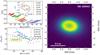Fig. 1

GRAVITY observations and best-fit model for HD 100453. Top left: squared visibilities as a function of spatial frequency. Colors refer to the different baselines. The inset presents the (u, v) plane coverage of the observations. Bottom left: closure phases as a function of the average spatial frequency. The various colors refer to the different triplets. Right panel: best-fit model.

3 Inner disks probed by VLTI/GRAVITY

The analysis of the inner disk geometries relies on the framework introduced by Lazareff et al. (2017). First, we fit the stellar SED to derive the disk K-band flux (Sect. 3.1). This parameter is required as an input for our parametric disk models that we fit to the GRAVITY data in order to derive the geometry of the inner disk of particular interest in this paper, namely its inclination and position angle (Sect. 3.2).

3.1 SED modeling

For each target we fit the photometric data points with two blackbodies B(ν, T) representing the stellar flux and the inner disk flux. The total flux density at frequency ν_k is given by $F (ν_{k}) = (F_{s V} \frac{B (ν_{k}, T_{eff})}{B (ν_{V}, T_{eff})} + F_{d K} \frac{B (ν_{k}, T_{dp})}{B (ν_{K}, T_{dp})}) \times 10^{- 0.4 A_{V} r_{k}},$ $\begin{equation*}F(\nu_k)=\left(F_{\mathrm{s}V}\frac{B(\nu_k,T_{\mathrm{eff}})}{B(\nu_V,T_{\mathrm{eff}})} + F_{\mathrm{d}K}\frac{B(\nu_k,T_{\mathrm{dp}})}{B(\nu_K,T_{\mathrm{dp}})}\right)\times10^{-0.4A_Vr_k},\end{equation*}$ (1)

where k ∈{1, …, 10} is an index for the photometric bandpasses; ν_k, ν_V, and ν_K are the mean frequencies of the k^th, V, and K band filter profiles, respectively; T_eff is the stellar effective temperature as presented in Table 1. r_k = A_k∕A_V is the extinction coefficient based on the extinction law of Cardelli et al. (1989). We adopt R_V = 3.1.

The fit parameters therefore are: F_sV, the stellar flux in the V band; F_dK, the thermal dust emission in the K band; the dust temperature T_dp, and A_V, the total extinction in the V band.

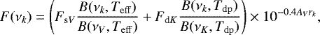
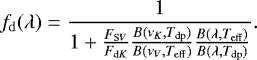
Due to numerical reasons, we fit for the logarithms of F_{s V}, F_{d K}, and T_dp (Lazareff et al. 2017). First, we applied a shuffled complex evolution (SCE) algorithm (Duan et al. 1993) to find the set of parameters that is minimizing the χ² map¹. This solution was used as a starting point for a Markov chain Monte Carlo (MCMC) sampler emcee (version 3.0.2; Foreman-Mackey et al. 2013), with 200 walkers and 10 000 steps to estimate the variances of model parameters. We discarded the first 1000 steps of each walker as the burn-in phase of the sampler; the convergence of the walkers was confirmed by visual inspection of the chains. To minimize the correlation among the resulting samples, we continued using only every 40^th step of the final chains. This provided 45 000 modelings of posterior samples for each target. We adopt the median and the 68% confidence interval as the final estimate for the fit parameters. An example SED fit for HD 100453 is presented in Fig. 2 and the best-fit parameters for all our targets are listed inTable 2. From these SED fits, we derived the flux contribution of the disk, f_d (λ) to the integrated flux at wavelength λ as $f_{d} (λ) = \frac{1}{1 + \frac{F_{S V}}{F_{d K}} \frac{B (ν_{K}, T_{dp})}{B (ν_{V}, T_{eff})} \frac{B (λ, T_{eff})}{B (λ, T_{dp})}} .$ $\begin{equation*}f_{\mathrm{d}}(\lambda) = \frac{1}{1 + \frac{F_{\mathrm{S}V}}{F_{\mathrm{d}K}}\frac{B(\nu_K,T_{\mathrm{dp}})}{B(\nu_V,T_{\mathrm{eff}})}\frac{B(\lambda,T_{\mathrm{eff}})}{B(\lambda,T_{\mathrm{dp}})}}.\end{equation*}$ (2)

This fraction is equivalent to the contribution of the second term in Eq. (1) to the total flux density, at a given wavelength λ. This contribution factor is required as an input parameter and initial value to our parametric models for the GRAVITY data and we evaluated Eq. (2) at the approximate central wavelength of the GRAVITY instrument at λ₀ = 2.25 μm (Table 2).

3.2 Parametric modeling of GRAVITY observations

We modeled the complex visibilities V (u, v, λ) using a combination of stellar (s), circumstellar (c), and halo (h) contributions. The halo mimics the contribution from an extended, over-resolved component due to scattered light. Models are fit to both squared visibilities and closure phases simultaneously.

We considered radial brightness distributions for the circumstellar component varying between a Gaussian profile and a Lorentzian profile. The model, of half-flux semi major axis a, is convolved with a kernel of semi major axis a_k, enabling us to describe rings of different widths as well as ellipsoids. All models include modulation amplitudes to first order m = 1. The model parameters are defined in Table 3 and a detailed description of the models can be found in Appendix B.1. Following the analysis of Lazareff et al. (2017), we added an extra term of ${(\frac{f_{c} - f_{d}}{σ_{f_{d}}})}^{2}$ $\begin{equation*}\left(\frac{f_{\mathrm{c}}-f_{\mathrm{d}}}{\sigma_{f_{\mathrm{d}}}}\right)^2\end{equation*}$ (3)

to the evaluation of χ². This assumption that f_d and f_c measure the same quantity helps to break the size-flux degeneracy of the model and to reduce the standard error of the disk half-light radii (see Sect. 3.4 of Lazareff et al. 2017). $σ_{f_{d}}$ $\sigma_{f_{\mathrm{d}}}$ refers to the uncertainty of the fractional flux contribution from the circumstellar disk at 2.25 μm (see Sect. 3.1 and Table 2).

We carry out an initial iteration of the SCE algorithm on the binned data to find the global minimum of the χ² map. The contributions of the squared visibilities and the closure phases to the combined χ² statistics were analyzed, and weighting factors were introduced such that (a) the χ² contributions for both squared visibilities and closure phases are the same and (b) the reduced χ² value is close to unity. After applying these weighting factors, the SCE algorithm was carried out again for both scenarios (a) and (b), and the results were used asstarting point for an MCMC. We used flat priors for all parameters as indicated in Table 3. Even though PA_in ∈ [0°, 180°] we allowed values in the range [−360°, 360°] for the fitting procedure. This allows continuous posterior distributions that do not exhibit any phase jumps when the true position angle is close to 0° or 180°. The final posterior distributions for PA_in were resampled such that the median value resided in the interval [0,180]. We used 200 walkers that are sampling 10 000 steps each. We discarded the first 1000 steps of each chain as burn-in phase and continue using every 40^th sample fromthe remaining posterior distributions. This provided 45 000 uncorrelated samples as our final posterior distribution. The MCMCwas carried out for both scenarios (a) and (b) and we used the median of the posterior distribution from method (b) as our best-fit model and derived associated uncertainties from the 68% confidence intervals generated by method (a).This procedure is analogous to the methodology described in Lazareff et al. (2017) and GRAVITY Collaboration (2019).

The physical quantities that correspond to the best-fit parameters, such as the half-flux radius, a, and the inner disk orientations, are presented in Table 4. Appendix B.1 provides the best-fit parameters (Table B.1), best-fit model maps (Fig. B.1) and comparison between best-fit model and observations(Fig. B.2).

Table 2

Results of our SED fits.

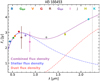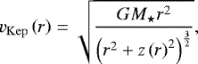
Fig. 2

SED fit for HD 100453. The circles represent the photometry and the solid purple curve, the best SED model from the MCMC posterior distribution. The model consists of two individual blackbody components that are visualized by the dashed lines: the blue curve represents the stellar flux density whereas the red curve shows the flux density of the circumstellar dust. The dotted line indicates the GRAVITY reference wavelength of 2.25 μm, at which we evaluate the dust flux contribution.

Table 3

Model parameter and priors of the MCMC fit to the GRAVITY data.

3.3 Critical view on geometric parameters uncertainties

We assessed how the uncertainties of our derived geometric parameters depend on the observational setup, in particular, the (u, v) plane coverage and the angular size of the disk. The results from this analysis are visualized in Fig. 3.

The (u, v) plane coverage, C_uv, was assessed geometrically. For each of the individual unbinned exposures we drew a circle for each baseline with a radius of 5 m around each measurement in the (u, v) plane. C_uv was determined as the fraction of area that was covered by these circles to the full area of a circle with the longest available baseline of 130.2 m as its radius. Accordingly, C_uv ∈ [0, 1] and the larger its value, the better the fractional coverage of the (u, v) plane. Both inclination and position angle are poorly constrained for the datasets with a scarcely sampled (u, v) plane. In the most extreme cases, we find uncertainties of up to 25° and 60° in inclination and position angle, respectively. For example, the observations of LkHα 330 have a very scarce (u, v) plane, yielding the large uncertainties of its inner disk inclination. The magnitude of these uncertainties decreases the larger C_uv, that is, the better the (u, v) plane is sampled. In the best constrained cases, we have uncertainties on the order of a few degrees.

For a few targets with C_uv < 0.05 though, we obtain a similarly low uncertainty. The reason for this good performance despite the scarce coverage of the (u, v) plane can be explained by the angular size of the environment that we try to resolve. As shown in the right panel of Fig. 3 there is a clear anticorrelation between the determined disk half-flux radius, a, and the uncertainties of the geometric parameters: the smaller the inner disk extent, the more difficult it is to derive its orientation. As the disk sizes depend on the stellar temperatures, the geometries for the Herbig AeBe stars are usually better constrained than for the T Tauri stars. There is one outlier, HD 139614, for which we measure the largest half-flux radius among the sample with ${4.75}_{- 0.42}^{+ 0.55}$ $4.75^{+0.55}_{-0.42}$ mas yet the uncertainties in inclination and position angle are comparably large, probably because the disk is observed almost face-on, which makes it challenging to precisely constrain inclination and position angle, or alternatively, because it is too resolved.

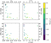Fig. 3

Uncertainties of the inner disk geometric parameters (i_in, PA_in) as a functionof (u, v) plane coverage, C_uv, and the disk half-flux radius, a. The colors indicate the stellar luminosity.

4 Outer disks probed with ALMA CO line data

In this section, we estimate the outer disk geometrical parameters by fitting gas velocity maps. While dust continuum observationsof our sample are available, some of them show substructures with significant asymmetry that could affect our estimates of the outer disk inclination and position angle. We therefore chose to model the velocity field of the rotating outer disk, assumed to be in Keplerian motion and considering its morphology as a conical surface (Teague et al. 2018).

4.1 Methodology

We collapsed the CO line data cubes using the quadratic collapsing method as implemented in the bettermoments Python library (Teague & Foreman-Mackey 2018). We masked out pixels with low signal-to-noise ratios in the peak line intensity after the calculation of the line center velocity, v₀. The magnitude of this clipping parameter was determined by visual inspection of the v₀ maps. An example moment map for HD 100453 is presented in the upper right panel of Fig. 4. We present the obtained velocity profiles for all targets in Fig. C.1.

For each target we fit the collapsed rotation profiles with the eddy Python tool (Teague 2019). We utilized the thick disk model, whose projected velocity profile is parametrized by $v_{proj} (r, ϕ) = v_{Kep} (r) \cos (ϕ) \sin (i_{out}) + v_{LSR}$ $\begin{equation*}v_{\mathrm{proj}}\left(r,\phi\right)=v_{\mathrm{Kep}}\left(r\right)\cos\left(\phi\right)\sin\left(i_{\mathrm{out}}\right)+v_{\mathrm{LSR}}\end{equation*}$ (4)

with Keplerian velocity $v_{Kep} (r) = \sqrt{\frac{G M_{⋆} r^{2}}{{(r^{2} + z {(r)}^{2})}^{\frac{3}{2}}}},$ $\begin{equation*}v_{\mathrm{Kep}}\left(r\right)=\sqrt{\frac{GM_{\star} r^2}{\left(r^2+z\left(r\right)^2\right)^{\frac{3}{2}}}},\end{equation*}$ (5)

the radius-dependent emission surface $z (r) = z_{0} {(\frac{r}{1 \hbox $^{''} $})}^{ψ},$ $\begin{equation*}z\left(r\right)=z_0\left(\frac{r}{1\hbox{$^{\prime\prime}$}}\right)^{\psi},\end{equation*}$ (6)

and the outer disk polar angle, ϕ in the disk-frame cylindrical coordinates. We use the local standard-of-rest (LSR) frame as a reference for radial velocities. The LSR is a point that has a velocity equal to the average velocity of stars in the solar neighborhood.

The fit parameters are: the outer disk inclination, i_out; the position angle of the outer disk, PA_out, defined from north to the redshifted part in an easterly direction; the systemic velocity v_LSR (the velocity of the star along the line of sight in the LSR frame); and the emission surface parameters z₀ and ψ. The outer position angle, PA_out, is uniquely defined within the interval [0°, 360°], whereas the outer inclination is bounded by [−90°, 90°]. To facilitatea proper comparison with the inner disk geometries we projected the outer disk inclinations to [0°, 90°] after the fitting. As there is a degeneracy between M_⋆ and i_out, we fixed thestellar mass for each target to the mean value from Table 1. The reported mass uncertainties were estimated after the fit of the outer disk by a Monte Carlo approach, exploiting the known 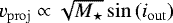$v_{proj} \propto \sqrt{M_{⋆}} \sin (i_{out})$ $v_{\mathrm{proj}}\propto \sqrt{M_{\star}}\sin\left(i_{\mathrm{out}}\right)$ dependency.

Due to beam smearing effects, we applied an inner mask of at least one beam major axis before proceeding with the fit. We further performed a down-sampling of the data to only fit spatially uncorrelated pixels, which additionally accelerates the fitting procedure. The fit was implemented using emcee, and we used 100 walkers with 4000 steps from which the first 2000 were discarded asburn-in phase. The MCMC fitting was repeated, using the marginalized posteriors of the first iteration as a starting value and again the initial 2000 steps of each chain were discarded. This provided 200 000 samples of our final posterior distribution. As the uncertainties might be underestimated, we performed a rescaling of the uncertainty map that was generated with bettermoments. The rescaling factor was calibrated to obtain a reduced χ² value of 1. The full MCMC process was repeated with these rescaled uncertainties. We adopted the median of the marginalized posterior distributions from this second fit as the best-fit parameters for the outer disk and used the 68% confidence intervals as corresponding uncertainties.

We confirmed the accuracy of our best fit models by visual inspection of iso-velocity contours plotted for the individual channel maps (Fig. 4, bottom), especially relevant for highly-inclined disks.

Table 4

Inner and outer disk geometries of our sample.

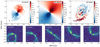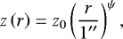
Fig. 4

Velocity maps and model fits to the ALMA CO line data of HD 100453. In all images north points up and east to the left. Top left: quadratically collapsed moment map derived with bettermoments. Top center: best-fit Keplerian disk model derived with the eddy tool. Top right: residuals after subtraction of the model from the data. Bottom panels: iso-velocity contours of the best-fit model plotted for the individual channel maps of the data cube.

4.2 Outer disk geometries

An example of the fit outer disk model and the corresponding residuals for HD 100453 is presented in Fig. 4. For all targets, we report the best-fit position angles, and outer disk inclinations that in addition consider the additional source of uncertainty from the stellar masses, in Table 4. The full output of the eddy Keplerian disk models to the ALMA data is listed in Table C.1. The uncertainties reported in this table represent the statistical errors that originate from the marginalized posterior distributions of the MCMC and do not include the mass uncertainties that need to be propagated to the derived inclinations. For some targets significant features are present after the subtraction of the velocity profile, in particular the residuals obtained for HD 100453, UX Tau A and CQ Tau, exhibit prominent spiral structures (e.g., Rosotti et al. 2020; Ménard et al. 2020; Wolfer et al. 2021). A detailed analysis of the morphology of the residuals from the fitting procedure on the full sample will be presented in a forthcoming publication (Wölfer et al., in prep.).

5 Inner and outer disk misalignments

5.1 Misalignment angles

We combine the results from the GRAVITY and ALMA data to probe potential misalignments between inner and outer disk geometry. To that end, we calculate a misalignment angle Δθ as a function of inner and outer inclinations, i_in and i_out, and position angles, PA_in and PA_out (see e.g., Fekel 1981; Min et al. 2017): $\begin{array}{l} Δ θ (i_{in}, {PA}_{in}, i_{out}, {PA}_{out}) \\ = \arccos [\sin (i_{in}) \sin (i_{out}) \cos ({PA}_{in} - {PA}_{out}) \\ + \cos (i_{in}) \cos (i_{out})] . \end{array}$ $\begin{eqnarray*}&& \Delta\theta(i_{\mathrm{in}},\mathrm{PA}_{\mathrm{in}},i_{\mathrm{out}},\;\mathrm{PA}_{\mathrm{out}})\nonumber\\&& \quad =\arccos \left[\sin\left(i_{\mathrm{in}}\right)\sin\left(i_{\mathrm{out}}\right)\cos\left(\mathrm{PA}_{\mathrm{in}} - \mathrm{PA}_{\mathrm{out}}\right) \right.\\&& \qquad \left. + \cos\left(i_{\mathrm{in}}\right) \cos\left(i_{\mathrm{out}}\right)\right].\nonumber\end{eqnarray*}$ (7)

This misalignment angle Δθ corresponds to the angle between the two normal vectors defined by the planes of the inner and outer disk, respectively. As introduced in Sect. 3, we cannot tell which side of the inner disk is closer to the observer and which is farther away. Accordingly, two potential misalignment angles need to be calculated that are representing each of the two scenarios. We define these two possibilities as $Δ θ_{1} = Δ θ (i_{in}, {PA}_{in}, i_{out}, {PA}_{out})$ $\begin{equation*}\Delta\theta_1=\Delta\theta(i_{\mathrm{in}},\mathrm{PA}_{\mathrm{in}},i_{\mathrm{out}},\mathrm{PA}_{\mathrm{out}})\end{equation*}$ (8)

and $Δ θ_{2} = Δ θ (i_{in}, {PA}_{in} + 180^{°}, i_{out}, {PA}_{out}) .$ $\begin{equation*}\Delta\theta_2=\Delta\theta(i_{\mathrm{in}},\mathrm{PA}_{\mathrm{in}}+180^{\circ},i_{\mathrm{out}},\mathrm{PA}_{\mathrm{out}}).\end{equation*}$ (9)

We estimated the uncertainties on the misalignment angles by a Monte Carlo approach, which randomly selected 200 000 samples from the posterior distribution of each required parameter. The median of this resulting distribution and the 68% confidence interval were selected as final values and uncertainties of the misalignment angles. The results of this analysis are presented in Table 4.

Figure 5 compares inner and outer inclinations (left panel) and position angles (right panel), respectively. The dashed lines indicate the values for which the inner and outer inclination and position angle are equal. Due to the uncertainty of the inner disk position angle, we present both solutions with PA_in ∈ [0°, 180°] (Δθ₁) as measured from the GRAVITY observables and PA_in + 180° (Δθ₂). If both the inclination and either of the two position angle solutions overlap with the dashed lines, it is possible that inner and outer disks are well aligned: this is supported for GM Aur, IP Tau, PDS 70, RX J1615, and SZ Cha within the 68% confidence intervals. For the remaining targets, our data is indicating that inner and outer disks exhibit a possible misalignment between inner and outer disk regions, which significance will be discussed in the following section.

5.2 Significance assessment

As Δθ ∈ [0°, 180°] and only configurations with perfectly aligned inner and outer disk geometries yield Δθ = 0, the derived misalignment angles usually deviate from zero, even within the provided uncertainties. It is therefore difficult to conclude from these angles, whether a disk is significantly misaligned or not. To properly test this underlying question in a statistical framework, we utilized an hypothesis testing approach. As a null hypothesis we assumed that the inner and outer disk are perfectly aligned, that is, i_in = i_out and PA_in = PA_out. The outer disk inclination and position angle are in most cases better constrained than the inner disk geometry. In addition to the posterior distributions of i_out and PA_out we shifted the posterior distributions of i_in and PA_in such that the median of the corresponding inner and outer distributions agreed. This simulates perfectly aligned inner and outer disks while accounting for the uncertainties that arise from the data and model fitting. From these simulated posterior distributions we calculated the misalignment angles $Δ θ_{1}^{sim}$ $\Delta\theta_1^{\mathrm{sim}}$ and $Δ θ_{2}^{sim}$ $\Delta\theta_2^{\mathrm{sim}}$ . These distributions describe how a perfectly aligned disk geometry would manifest in the fit results and derived parameters.

To test if our null hypothesis holds (i.e., the inner and outer parts of the analyzed disks are well aligned), we assessed how much the actual posterior distributions Δθ₁ and Δθ₂ and the simulations performed for the null hypothesis $Δ θ_{1}^{sim}$ $\Delta\theta_1^{\mathrm{sim}}$ and $Δ θ_{2}^{sim}$ $\Delta\theta_2^{\mathrm{sim}}$ were alike. We performed a Kolmogorov-Smirnov (KS) test and used the KS distance D_KS ∈ [0, 1] as a measure for the significance of the misalignment. The details of this framework are explained in Appendix D.

A value of D_KS close to zero indicates that inner and outer disks are almost perfectly aligned and D_KS close to unity indicates a significant misalignment. This framework naturally assigns lower values of D_KS to targets with loosely constrained geometries (i.e., broad distributions of Δθ₁ and Δθ₂). That way, it can be avoided that objects with large parameter uncertainties get misclassified as significantly misaligned with D_KS close to unity. On the other hand, large uncertainties do not necessarily provide D_KS values close to zero as the empirical distribution functions of relatively broad distributions can vastly differ if the medians of both distributions are distinct. We thus expect targets whose geometry is insufficiently characterized to exhibit intermediate values of D_KS ~ 0.5. For that reason we qualitatively identified three regimes with

(A)
0.9 < D_KS ≤ 1: targets that seem to exhibit significant misalignments between inner and outer disk structures;
(B)
0.3 ≤ D_KS ≤ 0.9: ambiguous targets, whose misalignment status is difficult to evaluate based on the current data;
(C)
and 0 ≤ D_KS < 0.3: targets that show no significant signs of misalignments.

Our goal here is to qualitatively distribute the systems in categories of disks that are more or less likely to be misaligned than others. Whereas targets in categories (A) and (C) provide strong statistical evidence to be either aligned or misaligned, we do not have conclusive evidence that significantly supports either state for the targets in the regime (B). We note that we use the KS distance D_KS instead of the p-values, as the latter are all too small to be used to categorize the disks, possibly due to the size of our sample.

The numerical values of the Kolmogorov-Smirnov distances for all targets are listed in Table 4 and visualized in Fig. 6. The figure presents D_KS sorted from best (bottom) to least (top) agreement with the null hypothesis. Histograms of the simulated and actual misalignment angle distributions can be found in Fig. D.1. Based on the selection criteria from Sect. 5 we find that SZ Cha, PDS 70, IP Tau, GM Aur, and RX J1615 show no significant signs for misalignments between inner and outer disks. This is in good agreement with the inclinations and position angles that are presented in Fig. 5: all of the aforementioned targets are compatible with the dashed lines that represent agreement of inner and outer disk orientations. On the other hand, V1366 Ori, HD 100453, CQ Tau, HD 142527, RY Lup, and V1247 Ori exhibit values of D_KS close to unity, indicative of significant misalignments present in these systems. The remaining targets fall into category (B), for which we cannot conclusively tell whether a misalignment is present or not.

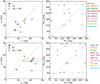Fig. 5

Misalignments between inner and outer disks in our sample of transition disks. The upper and bottom panels show the misalignments for the most massive stars of our sample (Herbig Ae/Be and intermediate-mass T Tauri stars) and for the T Tauri stars, respectively. Left panels: comparison of outer and inner disk inclinations. The dashed line indicates perfect alignment in inclination. Right panels: same as left panel but for inner and outer disk position angles. As we do not know the true orientation of the inner disk, we present both possibilities for the inner disk near sides. The full-colored markers represent the position angles from the GRAVITY fits and the white markers with the colored edges have an additional offset of 180°.

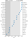Fig. 6

KS statistics testing the null hypothesis of perfectly aligned disk geometries. From bottom to top the targets are sorted from best (D_KS = 0) to worst agreement (D_KS = 1) with the null hypothesis. The different shades of background color indicate targets with no significant misalignment (left), significant misalignment (right) and dubious cases in the middle.

6 Shadows in scattered light images

Our targets were observed with VLT/SPHERE in scattered light, that is sensitive to illumination and shadowing effects. It is therefore informative to discuss these images in light of the inner disk orientations and misalignment angles derived before and check whether our predictions match the presence of shadows in scattered light images. For all targets, a gallery of this archival imagery is presented in Fig. E.1, and subsets of images are shown in Figs. 7 and 8. Each pixel in the disk images is scaled with squared radial distance to the star to account for the drop off in stellar illumination with increasing separation from the star and enhance faint features. We note that the image scaling does not take into account the geometry of the scattering surface which would be needed to derive an accurate morphology of the observed features. A plethora of substructures is visible for the transition disks of our sample that were discussed in the literature or are the subject of forthcoming publications (references given in Appendix E).

6.1 Methodolody

For targets that exhibit significant misalignments and the ambiguous cases, we further predict the locations of the shadows that depend on the morphology of the inner disk, and on the height of the scattering surface of the outer disk (Z_scat). This analysis follows the framework proposed by Min et al. (2017) and further used in Benisty et al. (2018). For given orientations of the inner and outer disk, and assuming Z_scat, the line connecting the shadows can be defined with its position angle 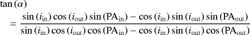$\begin{array}{l} \tan (α) \\ = \frac{\sin (i_{in}) \cos (i_{out}) \sin ({PA}_{in}) - \cos (i_{in}) \sin (i_{out}) \sin ({PA}_{out})}{\sin (i_{in}) \cos (i_{out}) \cos ({PA}_{in}) - \cos (i_{in}) \sin (i_{out}) \cos ({PA}_{out})} \end{array}$ $\begin{eqnarray*}&&\tan\left(\alpha\right)\nonumber\\&&\quad =\frac{\sin\left(i_{\mathrm{in}}\right)\cos\left(i_{\mathrm{out}}\right)\sin\left(\mathrm{PA}_{\mathrm{in}}\right) - \cos\left(i_{\mathrm{in}}\right)\sin\left(i_{\mathrm{out}}\right)\sin\left(\mathrm{PA}_{\mathrm{out}}\right)}{\sin\left(i_{\mathrm{in}}\right)\cos\left(i_{\mathrm{out}}\right)\cos\left(\mathrm{PA}_{\mathrm{in}}\right) - \cos\left(i_{\mathrm{in}}\right)\sin\left(i_{\mathrm{out}}\right)\cos\left(\mathrm{PA}_{\mathrm{out}}\right)}\end{eqnarray*}$ (10)

and offset in declination with respect to the star $η = \frac{Z_{scat} \cdot \cos (i_{in})}{\cos (i_{out}) \sin (i_{in}) \sin ({PA}_{in}) - \cos (i_{in}) \sin (i_{out}) \sin ({PA}_{out})} .$ $\begin{equation*}\eta = \frac{Z_{\rm{scat}} \cdot \cos\left(i_{\mathrm{in}}\right)}{\cos\left(i_{\mathrm{out}}\right)\sin\left(i_{\mathrm{in}}\right)\sin\left(\mathrm{PA}_{\mathrm{in}}\right) - \cos\left(i_{\mathrm{in}}\right)\sin\left(i_{\mathrm{out}}\right)\sin\left(\mathrm{PA}_{\mathrm{out}}\right)}.\end{equation*}$ (11)

As explained previously, depending on whether the near sides of the inner and outer disk match, these equations provide two sets of solutions. For all targets we assumed a fixed scattering height of Z_scat∕R = 0.1 as done by Min et al. (2017). The radial separation to the star, R, at which weconsider the scattering surface was determined by visual inspection of the scattered light images. We propagated the uncertainties of the inner and outer geometric disk parameters to obtain posterior distributions of α and η for each target.

6.2 Systems with significant misalignments

Our analysis predicts misalignments for six targets, HD 100453, HD 142527, CQ Tau, V1247 Ori, V1366 Ori and RY Lup, that we discuss in the following. For these, we show in Fig. 7 the two families of shadows in blue and orange, with 1000 randomly drawn samples from our posterior distributions of α and η.

HD 100453

This system exhibits dark lines in the east and the west. Ellipse fitting of the scattered light ring led to an outer disk inclination of ~ 38° and position angle of ~ 142° (Benisty et al. 2017). An inner disk inclination of ~48° and positionangle of ~80° were considered to reproduce the observed shadows, leading to a misalignment angle of ~ 72°. These values are in good agreement with our measurements: i_out ≈ 34°; PA_out ≈ 324°, and i_in = 46° ± 1°; PA_in = 82° ± 1°, yielding misalignment angles of Δθ₁ = 67° ± 1° and Δθ₂ = 41° ± 1°. As evident in Fig. 7, the solutions indicated with blue (Δθ₁) lines perfectly fit the location of the shadows. For the calculation of α and η, we assumed R = 40 au, yielding Z_scat = 4 au, as in Min et al. (2017).

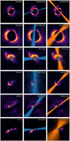Fig. 7

Left: scattered light images. Middle, right: same, with predicted lines connecting putative shadows based on both potential misalignment configurations, Δθ₁ and Δθ₂, respectively. The colored lines are 1000 randomly drawn samples from our posterior distributions that describe the shadow locations. The gray circles indicate the coronagraph.

HD 142527

The disk around this object also exhibits dark regions in the north and southeast of the star (see e.g., Fukagawa et al. 2006; Avenhaus et al. 2017). Marino et al. (2015) derived that inner and outer disks must be misaligned by 70°, with the inner disk position angle of −8°, to explain the observed morphology. This is marginally consistent with the position angle of PA_in = 15° ± 7° and the misalignment angle Δθ₁ = 59° ± 3° that we derived. Nevertheless, our analysis clearly confirms a strong misalignment between inner and outer disks. The shadow predictions for Δθ₁ as presented in Fig. 7, computed with R = 175 au, are in very good agreement with the observed shadow lanes.

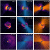Fig. 8

Predicted shadows for ambiguous cases that exhibit shadows in scattered light. The figure elements and image orientations are the same as for Fig. 7.

CQ Tau

The spiral structure seen in scattered light data of CQ Tau was presented by Uyama et al. (2020b). In the SPHERE data presented in this work, two dark regions are apparent in the south and in the west (Benisty et al., in prep.), at similar locations as the drop in peak intensity of the CO isotopologues seen in ALMA observations(Ubeira Gabellini et al. 2019; Wolfer et al. 2021). We derived an inner and outer disk inclination of 23° ± 3° and 32° ± 1° with associated position angles of $140_{- 9}^{+ 7}$ $140^{+7}_{-9}$ ° and 234° ± 1°, respectively, indicating a significant misalignment. For $Δ θ_{1} = 44_{- 3}^{+ 4}$ $\Delta\theta_1=44^{+4}_{-3}$ ° the predicted shadows with R = 15 au partly agree with the darker regions observed in scattered light (Fig. 7).

V1247 Ori

The disk shows asymmetries in scattered light (Ohta et al. 2016), in particular two spiral features well seen in the SPHERE data (Kraus et al., in prep.). ALMA continuum data show an asymmetric ring with a crescent and their analysis suggests a possible misalignment between inner and outer disk casting a shadow at a position angle of approximately 25° (Kraus et al. 2017). Our geometrical parameters suggest a significant misalignment between inner and outer disk components with $Δ θ_{1} = 15_{- 4}^{+ 3}$ $\Delta\theta_1=15^{+3}_{-4}$ ° and Δθ₂ = 59° ± 4°. For Δθ₁, the predicted locations of shadows (computed with R = 100 au) might trace some of the features observed in the scattered light image. Although the spiral structures makes it difficult to easily assess the presence of shadows, the shadows could be explaining why the spiral arms do not extend further. Neither solution of predicted shadows however agrees with a position angle of 25°.

V1366 Ori

The scattered light images, presented in de Boer et al. (2020), do not show any clear signatures of shadows but it might be due to the high inclination of the system, for which shadows could too narrow to be detected. We derive misaligment angles of Δθ₁ = 22° ± 6° or Δθ₁ = 108° ± 7°. The predicted shadow lanes, for R = 85 au, are presented in Fig. 7. Future observations with a higher signal-to-noise ratio and better angular resolution might reveal these predicted shadow lanes.

RY Lup

No clear shadows are visible in the scattered light images (Langlois et al. 2018), even though we derive a significant misalignment with D_KS = 0.98. Such nondetection can likely be attributed to the high inclination of the outer disk ( $i_{out} = 56_{- 5}^{+ 7}$ $i_{\mathrm{out}}=56^{+7}_{-5}$ °). Photometricand polarimetric observations of the system are indicative of a variable, highly inclined inner disk, with possible inner disk inclinations ranging from ~86° and ~55° (Manset et al. 2009). The latter estimate is marginally consistent with our estimate i_in = 46° ± 5°.

6.3 Ambiguous cases with known shadows

Three of the targets classified as ambiguous cases show shadow features in scattered light, while having intermediate values of D_KS. We present these cases below, and derive the predicted shadow positions in Fig. 8.

DoAr 44

North-south shadows are clearly evident in the scattered light data (Avenhaus et al. 2018). With an outer disk inclination and a position angle of 20° and 60°, respectively,estimated from ALMA dust continuum images, Casassus et al. (2018) used an inner disk inclination and position angle of 29.7° and 134°, respectively,to reproduce the shadows. The geometries obtained from our analysis agree very well with these values, and we find misalignment angles of Δθ₁ = 27° ± 9° and Δθ₂ = 39° ± 9°. We note that the solutions (with R = 20 au) for Δθ₁ reproduce well the shadows locations.

With D_KS = 0.68, we do not rank DoAr 44 as a significantly misaligned disk, yet the strong shadowing in scattered light is clearly supporting this. When inspecting the simulated and true posterior distributions of the misalignment angles (see Fig. D.1), it is obvious that the medians of these distributions are distinct. The rather large uncertainties for each of the distributions, however, do not allow for a value of D_KS > 0.9. Additional GRAVITY measurements that complete the (u, v) plane coverage should allow to derive better constraints on the inner disk inclination and especially its position angle that are currently dominating the uncertainties of the misalignment angles. These data would facilitate a confirmation of the misalignment hypothesis at higher statistical significance.

HD 135344 B

Even though this system shows clear signs of shadows in scattered light data, we do not find significant evidence for a misalignment with D_KS = 0.53. The large uncertainties for the inner disk parameters prohibited a higher value of D_KS. Interestingly, for that disk, three narrow shadow lanes, instead of two, were found, and are variable on timescales of (at least) months (Stolker et al. 2017). A misalignment angle of ~ 22° was inferred (Stolker et al. 2016), consistent with $Δ θ_{2} = 17_{- 6}^{+ 8}$ $\Delta\theta_2=17^{+8}_{-6}$ ° that we find. However, we find that while the shadow lanes associated with Δθ₂ (computed with R = 25 au) might explain two shadows, the morphology of the inner disk is likely too complex to be captured by our rather simplistic models.

HD 139614

More than half of the outer disk is not visible in scattered light. To generate such a broad shadow, the misalignment must be as small as 4° (Muro-Arena et al. 2020). The predicted inclination of the inner disk (20.6°) is in agreement with our findings 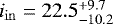$i_{in} = {22.5}_{- 10.2}^{+ 9.7}$ $i_{\mathrm{in}}=22.5^{+9.7}_{-10.2}$ °, while the predicted position angle (272°) differs from our estimate 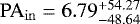${PA}_{in} = {6.79}_{- 48.64}^{+ 54.27}$ $\mathrm{PA}_{\mathrm{in}}=6.79^{+54.27}_{-48.64}$ °. However, the uncertainties on the inner disk position angle are very large, due to the fact that disk is nearly face-on. While $Δ θ_{1} = 27_{- 12}^{+ 13}$ $\Delta\theta_1=27^{+13}_{-12}$ ° predicts shadow lanes (with R = 30 au) over the disk area that is illuminated by stellar light, $Δ θ_{2} = 28_{- 12}^{+ 13}$ $\Delta\theta_2=28^{+13}_{-12}$ ° agrees muchbetter with the scattered light morphology.

In agreement with our derived misalignment angles and Kolmogorov-Smirnov statistics, none of the five targets in the category with aligned disks shows any significant shadow in scattered light.

7 Discussion

In the previous sections, we found that the predictions from our joint analysis of VLTI and ALMA observations are consistent with the presence of misalignment in at least 6 out of the 20 disks of our sample while 5/20 disks appear to have inner disks well aligned withtheir outer disks. Unfortunately, in nearly half of our sample (9/20 disks) a possible misalignment is difficult to assess. This is partly due to the limited angular resolution of VLTI insufficient to resolve the inner disk of T Tauri stars or due to the specific geometry of some disks. While our analysis can therefore not be conclusive on the occurrence rate of misalignments in transition disks, it sets the methodology for future higher quality observations of these disks. In the following, we discuss the possible origin of disk misalignments, in the light of the nature of these inner disks in transition disks.

Observational evidence for misalignments

The presence of misaligned disk regions, or more generally of warps in disks, has been long known, in particular from the modulation present in the photometric data of young stars. Most young stars are variable (Herbst et al. 1994; Herbst 2012) and a subclass of late-type objects, the so-called dippers, accounting for ~30% of the young stellar population (Cody & Hillenbrand 2018) show short duration extinction events, with highly variable photometric dips in both their occurrence timescales and shapes (e.g., Cody et al. 2014). These events were interpreted as being due to occulting dusty material very close to the star (McGinnis et al. 2015; Bodman et al. 2017). To hide part of the stellar surface, the dust shielding the star must be crossing our line of sight and therefore be moving on a very inclined orbit (Bouvier et al. 2003; Bodman et al. 2017). However, spatially resolved ALMA images of the outer disks of 24 dippers showed an isotropic distribution of inclinations, with some dipper disks close to face-on, indicating that disk misalignment might be quite common in young stars (Ansdell et al. 2018). In addition to photometric variations and shadows in scattered light images, there are further observational indications of misalignments in disks, such as different orientations of the dust continuum emission of transition disks (Francis & van der Marel 2020) or perturbed kinematics of gas (HCO+) emission (Loomis et al. 2017).

Origin of the misalignments

The dippers with periodic light curves, can be explained by the presence of an inclined magnetic field that induces a warp or misalignment in the innermost disk regions, that regularly crosses our line of sight (Bouvier et al. 1999). In aperiodic dippers, the stochastic extinction events must result from rapid changes in the inner disk structure and orientation that can produce asymmetric stellar occultations, but it is unclear what exactly is driving these changes. An unstable accretion regime leading to a magnetically-induced warp (Kurosawa & Romanova 2013), asymmetric density structures such as vortices induced by Rossby wave instabilities at the edge of a dead zone (Meheut et al. 2012; Flock et al. 2017), or dusty disk winds (Bans & Königl 2012) have been invoked. In variable intermediate-mass young stars (UX Ors), highly inclined dust clumps that sublimate close to the stars were suggested (Grinin et al. 1996) but their origin is not clear. It is difficult to constrain such scenarios with our observations, as simultaneous photometric and interferometric campaigns should be carefully planned to address this issue. However, we note that structural variability was already inferred in some objects, in particular in transition disks, from photometric, spectroscopic and interferometric studies (Espaillat et al. 2011, 2014; Chen et al. 2019).

Another scenario to consider is the presence of a massive companion that would induce a misalignment of specific disk radii. This other possibility appears as a natural one in transition disks as they show a dust-depleted cavity that can be carved by multiple planets (Bae et al. 2019) or by a stellar companion (Price et al. 2018). When the companion angular momentum is greater than the inner disk’s, the disk region within the companion’s orbit will be tilted (Xiang-Gruess & Papaloizou 2013; Matsakos & Königl 2017). Using 3D simulations, Nealon et al. (2018) similarly found that, for a planet massive enough to carve a gap, the inner and outer disk will be misaligned, and Bitsch et al. (2013) found that in some cases, the disk can have a higher inclination than the planet. In the extreme case of binary systems, the inner disk can even break and precess (Facchini et al. 2013), leading to a variety of misalignment angles that could induce narrow or broad shadows in scattered light (Facchini et al. 2018; Benisty et al. 2018). Significant misalignments can also be induced by secular precession resonances in the case of high stellar-companion mass ratio (Owen & Lai 2017). Interestingly, in the case of a triple system suchas HD100453, a massive planet located within the cavity can be brought to a high inclination via the Kozai-Lidoveffect and lead to an inner disk misalignment (Martin et al. 2016; Gonzalez et al. 2020; Nealon et al. 2020; Ballabio et al. 2021). While our observations are not sensitive to low mass companions, stellar binary companions of high mass ratio, within the field of view of the telescopes (250 mas for the ATs; 60 mas for the UTs), would have been detected in our interferometric observations. The detection limits available from direct imaging data in the inner regions (within transition disk cavities) are in general limited by the complexities of the disk structures and with the uncertainties in the evolutionary models considered, the current estimates are around a few to ~10 Jupiter masses (Asensio-Torres et al. 2021). So far, out of our sample, only PDS70 has directly imaged planets (Keppler et al. 2018)while yet-unconfirmed candidate companions were claimed in the cavities of LkCa15 and HD 100546 (Quanz et al. 2013; Sallum et al. 2015).

Finally, another possibility is that the misalignment is an outcome of earlier stages of star formation (Bate 2018). Bate et al. (2010) note that the inner disk could be misaligned with respect to the stellar rotation axis, due to the chaotic nature of star and disk formation. It was recently proposed that the outer disk could be misaligned as a result of late accretion events from material accreted with a misaligned angular momentum (Dullemond et al. 2019; Kuffmeier et al. 2021), a scenario possibly at play in SU Aur where both a large scale arm (Akiyama et al. 2019) and a misaligned inner disk are observed (Ginski et al. 2021). In the sample of transition disks that we studied in this paper, two targets within the “ambiguous” subset, HD 100546 and UX Tau A, show extended features in scattered light (Ardila et al. 2007; Ménard et al. 2020) but in the case of UX Tau A they seem well accounted for by a flyby.

Misalignment with respect to the stellar rotation axis

An interesting question which could help understand the cause for the misalignment, is whether in our sample of disks, it is the inner disk or the outer disk that is misaligned with respect to the stellar rotation axis. Within the transition disk sample analyzed in this paper, two objects are known dippers, LkCa15 (Alencar et al. 2018) and DoAr44 (Bouvier et al. 2020) and have been studied in great details. Alencar et al. (2018) find that LkCa15 must present an extended inner disk warp to reproduce the duration of the dips, and derive a stellar inclination i_⋆ larger than 65°, a value consistent with our estimate of the inner disk inclination ( $i_{in} = {61.0}_{- 20.8}^{+ 18.6}$ $i_{\mathrm{in}}=61.0^{+18.6}_{-20.8}$ °) although our estimate suffers large error bars. Spectro-polarimetric observations also confirm such a large inclination for the star (i_⋆ ≥ 70°; Donati et al. 2019). It is in any case, much higher than the inclination that we derive for the outer disk ( $i_{out} = {43.9}_{- 2.1}^{+ 2.3}$ $i_{\mathrm{out}}=43.9^{+2.3}_{-2.1}$ °) and that is obtained from continuum ALMA observations (50.16°± 0.03°; Facchini et al. 2020) and suggests that the outer disk is misaligned with respect to the star+inner disk system. Similarly, in DoAr 44, Bouvier et al. (2020) find that the stellar inclination is i_⋆ = 30° ± 5° in agreement with our estimate of the inner disk inclination. Finally, in another transition disk (and dipper) not included in our sample, RXJ1604.3-2130, Davies (2019) find that i_⋆ ≥ 61°, while its outer disk is seen almost face-on (Pinilla et al. 2018). It is unclear whether all transition disks have an inner disk sharing the same orientation as the star, but these three examples seem to suggest that the misalignment occurred on the outer disk. In these objects, it is likely that there is, in addition to a global misalignment of the inner disk, an additional warp due to an magnetic field inclined with respect to the stellar rotation axis (Sicilia-Aguilar et al. 2020).

Dependence on stellar properties

The three objects discussed above are at the same time, dippers and transition disks, and are surrounding T Tauri stars, for which a strong magnetic field shaping the innermost disk region can be inferred. In contrast, it is unclear whether Herbig AeBe stars host strong magnetic fields (Alecian et al. 2013) capable of warping the inner disk. However, it appears that shadows in scattered light, indirect tracers of disk misalignments, are predominant among the intermediate mass young stars, and in particular those with spiral arms and high near-infrared excess (Garufi et al. 2018), possibly hinting at another mechanism than in the T Tauri case. It is interesting to note that such a high near-infrared excess must result from a larger disk surface to reprocess the stellar light. This could imply that in these disks dust grains are lifted to higher altitude, possibly through a disk wind or due to the dynamical interaction with a massive companion.

Finally, we note that our current understanding of the nature of these inner disks in transition disk is limited by the complexity of the ongoing phenomena therein resulting in a strongly depleted cavity. In some cases, the dust in the inner disk even seems to be disappearing and rapidly replenished (e.g., Sicilia-Aguilar et al. 2020) and variable shadows (Stolker et al. 2017)indicate a highly dynamical structure. Other cases still show significant accretion rates (Manara et al. 2014) and accretion signatures similar to continuous disks (Bouvier et al. 2020). Given the complexity and the short dynamical timescales of the inner disk regions, it is remarkable that in several cases our parametric modeling of the VLTI observations of the inner disks matches so well the shadowing exhibited by the scattered light observations. One of the next steps forward will consist in studying these inner disks and the mass flow within the cavity simultaneously through high spectral and high angular observationsand if possible, follow the putative motions of shadows and/or substructures in the outer disk to constrain the origin of the misalignments.

8 Conclusions

We investigated misalignments between inner and outer disk regions of transitional disk systems using VLTI/GRAVITY and ALMA observations. The analysis is conducted for a sample of 20 transitional disks around stars of various masses and luminosities, comprising T Tauri stars with masses as low as 0.6 M_⊙ to Herbig stars with masses of up to 3 M_⊙. The geometries of the inner disk regions were constrained by parametric model fits to the squared visibilities and closure phases collected with GRAVITY. We fit ALMA molecular line velocity maps using a Keplerian disk model. From inner and outer disk orientations, we derived misalignment angles between the normal vectors of the planes of both disk components. We performed hypothesis testing in a Kolmogorov-Smirnov framework to assess whether the disks from our sample exhibited significant misalignments. For systems with significant misalignments or shadows observed in near-infrared scattered light, we simulated the positions of these shadows based on the orientations of the inner and outer disks.

Our main findings can be summarized as:

We find six systems whose outer and inner disk were significantly misaligned, 5 that appear to not have misalignments, and 9 targets for which we can not accurately evaluate this with the current data.
In those for which we find that the outer and inner disk are significantly misaligned: For HD 100453 and HD 142527, the predicted shadow positions are in great agreement with scattered light observations. For CQ Tau, the predicted shadow positions seems to probe parts of the disk that are less illuminated in scattered light. We do not find any evidence for shadows in the disks around V1247 Ori, V1366 Ori and RY Lup. Especially for the latter two systems this might be caused by the large inclination. Future observations at higher spatial resolution and with higher signal-to-noise ratio detections of these disks might reveal the shadow features that are predicted by our analysis.
Three disks around DoAr 44 and, HD 135344 B, and HD 139614 show dark regions in scattered light, even though we do not probe any significant misalignments with our analysis. This is mostly caused by the large uncertainties that we obtained for especially the inner disk geometries of these systems. In addition, the multiple shadow lanes and broad shadow regions in these disks are likely caused by complex physical processes that are not accurately modeled by our geometrical models.
With the current data available from VLTI, we can derive precise geometric constraints with uncertainties of a few degrees for the orientations of the inner disks of Herbig Ae/Be stars; we can measure the inner disk geometries of the T Tauri stars with marginal constraints of several tens of degrees. This correlation can be attributed to the angular size of the environment that needs to be resolved. Another important parameter for the quality of our fit results was the (u, v) plane coverage. Observations that only scarcely sampled this plane provided on average worse constraints for the inner disk inclinations and position angles.

We additionally discuss the possible origins of the misalignment in transition disks, although there is no consensus on the mechanisms responsible for it. As the nature of these inner disks in transition disk is very complex, future observing campaigns, at both high spectral and spatial resolution will be key to study the gas and dust content, structure, and dynamics therein, and help constrain the origin of the cavities and misalignments.

Acknowledgements

We are very grateful to Jaehan Bae, Paola Pinilla and Nicolas Kurtovic for insightful discussions. We thank the referee for a very constructive report that helped improve the quality of the manuscript. This paper makes use of the following ALMA data: ADS/JAO.ALMA#2011.0.00465.S, ADS/JAO.ALMA#2012.1.00158.S, ADS/JAO.ALMA#2012.1.00870.S, ADS/JAO.ALMA#2013.1.00498.S, ADS/JAO.ALMA#2013.1.00163.S, ADS/JAO. ALMA#2013.1.00592.S, ADS/JAO.ALMA#2013.1.01075.S, ADS/JAO.ALMA# 2015.1.00490.S, ADS/JAO.ALMA#2015.1.01301.S, ADS/JAO.ALMA#2015. 1.01600.S, ADS/JAO.ALMA#2015.1.00888.S, ADS/JAO.ALMA#2015.1. 00986.S, ADS/JAO.ALMA#2015.1.00192.S, ADS/JAO.ALMA#2016.A. 00026.S, ADS/JAO.ALMA#2016.1.00826.S, ADS/JAO.ALMA#2016.1.00344.S, ADS/JAO.ALMA#2017.A.00006.S, ADS/JAO.ALMA#2017.1.01404.S, ADS/JAO.ALMA#2017.1.01424.S, ADS/JAO.ALMA#2017.1.00449.S, ADS/JAO.ALMA#2018.1.01055.L, ADS/JAO.ALMA#2018.1.01255.S, ADS/JAO.ALMA#2018.1.01302.S. ALMA is a partnership of ESO (representing its member states), NSF (USA), and NINS (Japan), together with NRC (Canada), NSC and ASIAA (Taiwan), and KASI (Republic of Korea), in cooperation with the Republic of Chile. The Joint ALMA Observatory is operated by ESO, AUI/NRAO, and NAOJ. This project has received funding from the European Research Council (ERC) under the European Union’s Horizon 2020 research and innovation programme (grant agreements No. 101002188, No. 832428, No. 678194, No. 639889, No. 823823) and the Deutsche Forschungsgemeinschaft (DFG, German Research Foundation) – 325594231, FOR 2634/2. R.G.L. acknowledges support from Science Foundation Ireland under Grant No. 18/SIRG/5597. This research has made use of the Jean-Marie Mariotti Center Aspro and SearchCal services (available at http://www.jmmc.fr/aspro; http://www.jmmc.fr/searchcal). This research has used the SIMBAD database, operated at CDS, Strasbourg, France (Wenger et al. 2000). This work has used data from the European Space Agency (ESA) mission Gaia (https://www.cosmos.esa.int/gaia), processed by the Gaia Data Processing and Analysis Consortium (DPAC, https://www.cosmos.esa.int/web/gaia/dpac/consortium). This publication makes use of VOSA, developed under the Spanish Virtual Observatory project supported by the Spanish MINECO through grant AyA2017-84089. To achieve the scientific results presented in this article we made use of the Python programming language (Python Software Foundation, https://www.python.org/), especially the SciPy (Virtanen et al. 2020), NumPy (Oliphant 2006), Matplotlib (Hunter 2007), emcee (Foreman-Mackey et al. 2013), scikit-image (Van der Walt et al. 2014), scikit-learn (Pedregosa et al. 2012), photutils (Bradley et al. 2016), and astropy (Astropy Collaboration 2013, 2018) packages.

Appendix A Observing log

A.1 GRAVITY observations

We present the observational setup and observing conditions for all our observations in Table A.1. All observations were carried our in single field mode mode using either the UTs or ATs.

A.2 ALMA observations

For each target we search the ALMA archive for the CO isotopologue line data with the best combination of spatial resolution, spectral resolution and sensitivity. Generally the ¹²CO line is the brightest and thus chosen for our analysis, but in a few cases only the ¹³CO line was available. The properties of the ALMA line cube observations and references is presented in Table A.2. For most targets, the authors of the papers where these data were published provided the reduced fits files (PC). For GM Aur, HD 139614,SZ Cha and IP Tau, the datasets were downloaded directly from the ALMA archive (programs 2018.1.01055.L, PI Öberg; 2015.1.01600.S, PI Panic; 2013.1.00163.S, PI Simon; 2013.1.01075.S, PI Daemgen). For all these targets but GM Aur, the data were reduced using the provided calibration scripts and imaged using the tclean task with natural weighting.

A.3 Spectral energy distributions

The photometry collected from Tycho-2 (B and V bands), Gaia EDR3 (G_BP, G, and G_RP bands), USNO-B (R and I bands), 2MASS (J, H, and K bands) catalogs is presented in Table A.3.

Table A.1

Setup and weather conditions of the GRAVITY observations.

Table A.2

Basic properties of the ALMA line observations

Table A.3

Photometric data of the targets in our sample.

Appendix B GRAVITY inner disk modeling

In this section we present the parametric models that we use to fit the GRAVITY data. Sect. B.1 reiterates the main components of the analytical model derived by Lazareff et al. (2017) that is used to describe the observed complex visibilites.

B.1 Model description

B.1.1 Complex visibilities

We model the complex visibilities V (u, v, λ) as describedby Lazareff et al. (2017) using a combination of stellar (s), circum-stellar (c), and halo (h) contributions. For a proper derivation of the used model, the reader is referred to Sect. 3 of Lazareff et al. (2017). The final model is provided by $V (u, v, λ) = \frac{f_{s} {(λ_{0} / λ)}^{k_{s}} + V_{c} (u, v, λ) {(λ_{0} / λ)}^{k_{c}}}{(f_{s} + f_{h}) {(λ_{0} / λ)}^{k_{s}} + f_{c} {(λ_{0} / λ)}^{k_{c}}},$ $\begin{equation*}V(u,v,\lambda)=\frac{f_{\mathrm{s}}(\lambda_0/\lambda)^{k_{\mathrm{s}}}+V_{\mathrm{c}}(u,v,\lambda)(\lambda_0/\lambda)^{k_{\mathrm{c}}}}{(f_{\mathrm{s}}+f_{\mathrm{h}})(\lambda_0/\lambda)^{k_{\mathrm{s}}}+f_{\mathrm{c}}(\lambda_0/\lambda)^{k_{\mathrm{c}}}}\;,\end{equation*}$ (B.1)

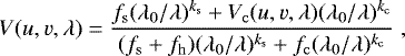
where λ₀ = 2.25 μm is defined as the GRAVITY reference wavelength as before; f_s, f_c, and f_h denote the fraction of the total flux at wavelength λ₀ within the VLTI field of view that originate from the star, the circumstellar material, and the halo component, respectively; and, k_s and k_c represent the spectral indices of stellar and circumstellar components, respectively.

Eq. B.1 assumes that the star is an unresolved point source for all baselines. V_c (u, v, λ) are the visibilities that are associated with the circumstellar dust. All three quantities f_s, f_c, and f_h are positive semi-definite and related by $f_{s} + f_{c} + f_{h} = 1 .$ $\begin{equation*}f_{\mathrm{s}}+f_{\mathrm{c}}+f_{\mathrm{h}}=1\;.\end{equation*}$ (B.2)

The fractional flux contribution f_h originates from a halo that is fully resolved at all the baseline configurations. This extended component mimics scattered light (e.g., Pinte et al. 2008).

The spectral dependence of the star and the circumstellar component is assumed to follow a power law whose spectral index at frequency ν is defined as $k = \frac{d \log_{10} (F_{ν})}{d \log_{10} (ν)} .$ $\begin{equation*}k=\frac{\mathrm{d}\log_{10}(F_{\nu})}{\mathrm{d}\log_{10}(\nu)}\;.\end{equation*}$ (B.3)

As the halo component is assumed to originate from scattered starlight, this component inhibits the same wavelength dependence – and therefore the identical spectral index – as the star. We derived the stellar spectral indices, k_s, at GRAVITY reference wavelength λ₀ = 2.25 μm, assuming blackbody emission with the host star temperatures reported in Table 1.

The closure phases that are corresponding to the disk model of Eq. (B.1) can be derived as $Φ (u_{1}, v_{1}, u_{2}, v_{2}, λ) = \arg (B_{123}) = \arctan (\frac{ℜ (B_{123})}{ℑ (B_{123})})$ $\begin{equation*}\Phi(u_1, v_1, u_2, v_2, \lambda) = \arg\left(B_{123}\right)= \arctan\left(\frac{\Re\left(B_{123}\right)}{\Im\left(B_{123}\right)}\right)\end{equation*}$ (B.4)

with the triple product $B_{123} (u_{1}, v_{1}, u_{2}, v_{2}, λ) = V (u_{1}, v_{1}, λ) V (u_{2}, v_{2}, λ) V^{*} (u_{1} + u_{2}, v_{1} + v_{2}, λ) .$ $\begin{equation*}B_{123}(u_1, v_1, u_2, v_2, \lambda)=V(u_1, v_1,\lambda) V(u_2, v_2, \lambda) V^*(u_1+u_2, v_1+v_2, \lambda)\;.\end{equation*}$ (B.5)

and with ℜ and ℑ refer to a complex number’s real and imaginary part, respectively, and ^* denotes the complex conjugate.

B.1.2 Disk model

A detailed analytical derivation of the complex visibilities associated with the models is presented in Sect. 3.6 of Lazareff et al. (2017) and we recall the main parameters in Table 3. With this prescription, we describe asymmetric ellipsoid and ring-like morphologies, and discuss in the following key parameters.

The parameter f_Lor ∈ [0, 1] describes the underlying radial profile of the emission: f_Lor = 0 correspondsto a Gaussian intensity profile that decays exponentially as exp (−r²), f_Lor = 1 describes a pseudo-Lorentzian profile that is proportional to r⁻³. Intermediate values of f_Lor refer to a combination of Gaussian and Lorentzian brightness distribution.

The parameter l_a is a measureof the half-flux extent of the disk. The parameter is connected via $l_{a} = \log_{10} (\frac{a}{1 mas})$ $\begin{equation*}l_a=\log_{10}\left(\frac{a}{1\,\mathrm{mas}}\right)\end{equation*}$ (B.6)

to the half-flux radius $a = (a_{r}^{2} + a_{k}^{2}),$ $\begin{equation*}a=\left(a_r^2+a_k^2\right)\;,\end{equation*}$ (B.7)

which is derived from the geometrical parameters a_r and a_k. a_r denotes the angular radius of the ring and a_k describes the angular radius of the kernel that is convolved with the disk geometry.

The parameter $l_{kr} = \log_{10} (\frac{a_{k}}{a_{r}})$ $\begin{equation*}l_{\mathrm{kr}}=\log_{10}\left(\frac{a_{\mathrm{k}}}{a_{\mathrm{r}}}\right)\end{equation*}$ (B.8)

captures the logarithmic ratio between these two variables. Accordingly, a value of l_kr < 0 corresponds to ring-like geometries with a_k ≪ a_r and l_kr > 0 creates ellipsoids with a_k ≫ a_r.

The pair of parameters c_j and s_j describe azimuthal modulation amplitudes that create azimuthal brightness asymmetries in the disk models. Those terms are required to describe well-resolved disks that are viewed at nonzero inclination. In cases such as these, the far side of the dust sublimation rim appears more luminous than the front side and azimuthal modulations are required for a proper description of the observed geometry. For each order m of modulation amplitudes that are included in the parametrization, one additional cosine c_j and a sine s_j term need to be considered.

The parameters that are most important within the scope of this work are $\cos (i_{in})$ $\cos\left(i_{\mathrm{in}}\right)$ and PA_in, which describe the inclination and position angle of the inner disk. From the GRAVITY observations, we cannot in general tell which side of the disk is closer to the observer (i.e., the front side) and which is farther away (i.e., the back side). Therefore, the inner disk inclination is defined as a positive angle in the range [0°, 90°] with i_in = 0° and i_in = 90° describing face-on and edge-on disk geometries, respectively. The position angle is defined on the interval PA_in ∈ [0°, 180°] and describes the positive rotation of the disk’s major axis with respect to north. One needs to keep in mind that a tuple of i_in and PA_in always refers to two potential physical configurations, which are mathematically represented by (i_in, PA_in) and (− i_in, PA_in). Without further information on the inner disk orientation it is not possible to break this degeneracy. This is considered when calculating misalignment angles as detailed in Sect. 5.

The model fitting results are given in Table B.1, with the best models shown in Fig. B.1. Fig. B.2 shows the observations and best-fit models.

Table B.1

Results of the model fits to the GRAVITY data.

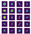Fig. B.1

Best-fit inner disk models from the GRAVITY observables. In all images north points up and east toward the left.

Fig. B.2

GRAVITY observables and model fits. In the upper left of each panel, the (u, v) plane coverage is shown. Each symbol corresponds to an individual exposures and the colors refer to the interferometric baselines. The other panels of the plot show the squared visibilities (right) and closure phases (left) for each baseline or triplet as a function of wavelength. The white markers with black contours represent the observational data and the black lines correspond to our best-fit model. The black markers on top of the lines indicate which curve corresponds to which exposure.

Appendix C ALMA data and best fit parameters

We present the velocity maps that were generated with the bettermoments tool in Fig. C.1. The best-fit parameters of our Keplerian disk models as introduced in Sect. 4 are presented in Table C.1. The corresponding residuals of the data and the best-fit eddy models will be discussed in a forthcoming publication (Wölfer et al., in prep.).

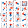Fig. C.1

ALMA line data of our targets. We present the quadratically collapsed moment maps that were created with bettermoments by quadratic collapsing of the frequency channels. The ellipse in the lower left of each panel indicates the beam size of the observation. For all images north points up and east to the left.

Table C.1

Results from the outer disk model fits of the ALMA line data cubes.

Appendix D Misalignment angles

To quantify the alikeness of the true and simulated misalignment distributions, we used Kolmogorov–Smirnov statistics. The Kolmogorov–Smirnov distance $D (F, G) = \max_{x} [\lvert F (x) - G (x) \rvert]$ $\begin{equation*}D(F,G)=\underset{x}{\max}\left[\lvert F(x)-G(x)\rvert\right]\end{equation*}$ (D.1)

measures the parameter x that maximizes the difference between two empirical distribution functions F and G, representing the samples X = {X₁, …X_n}~ F and Y = {Y₁, …Y_m}~ G. Accordingly, D(F, G) ∈ [0, 1] with D(F, G) = 0 indicates that both samples X and Y originate from the same underlying distribution. The stronger D(F, G) deviates from zero, the higher the likeliness that X and Y are not drawn from the same distribution.

This statistical framework can be applied to our problem as follows. Let $Δ θ_{1}^{sim} ~ F_{1}$ $\Delta\theta_1^{\mathrm{sim}}\sim F_1$ , $Δ θ_{2}^{sim} ~ F_{2}$ $\Delta\theta_2^{\mathrm{sim}}\sim F_2$ , Δθ₁ ~ G₁, and Δθ₂ ~ G₂ the (simulated) posterior distributions and corresponding empirical distribution functions. We define the final Kolmogorov–Smirnov distance between simulated and measured parameters as $\begin{matrix} D_{KS} : = \min { & \max [D (F_{1}, G_{1}), D (F_{2}, G_{2})], \\ \max [D (F_{1}, G_{2}), D (F_{2}, G_{1})]} \in [0, 1] . \end{matrix}$ $\begin{equation*}\begin{array}{@{}l@{}l}D_{\mathrm{KS}}:=\min\{&\max\left[D(F_1,G_1),D(F_2,G_2)\right],\\&\max\left[D(F_1,G_2),D(F_2,G_1)\right]\}\in[0,1]\;.\end{array}\end{equation*}$ (D.2)

It is insufficient if only one of the misalignment distributions Δθ₁ or Δθ₂ agrees with its simulated counterpart, that is, for perfect alignment it is not sufficient if for instance D(F₁, G₁) = 0 and D(F₂, G₂) = 1. For that reason, we calculate the maximum of both corresponding Kolmogorov–Smirnov distances.

Since the true orientation of the disk is unknown, we have to test both potential combinations, that is, $Δ θ_{1}^{sim}$ $\Delta\theta_1^{\mathrm{sim}}$ might either correspond to Δθ₁ or Δθ₂ and $Δ θ_{2}^{sim}$ $\Delta\theta_2^{\mathrm{sim}}$ to the respective remaining parameter. The minimum of these potential permutations allows to find the orientation that prefers our null hypothesis most. D_KS behaves as D(F, G) and a value close to zero can be interpreted as a confirmation of our null hypothesis, whereas a deviation from zero indicates a misalignment between inner and outer disk components. The magnitude of the deviation from zero further indicates the significance at which the null hypothesis must be rejected. The posterior distributions of our derived misalignment angles are presented inFig. D.1. The figure also shows the misalignment distributions that were simulated for a perfect alignment between inner and outer disk. The more both distributions deviate the higher the likelihood that our null hypothesis (i.e., the inner and outer disks are well aligned) needs to be rejected. The figure can be used to understand the associated values of D_KS that are presented in Table 4.

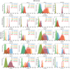Fig. D.1

Posterior distributions of the derived misalignment angles. We also present the simulated distributions for a perfectly aligned disk geometry. Good agreement of the true and simulated distributions indicates that inner and outer disk are well aligned. Deviations from this agreement are signs of potential misalignment.

Appendix E Scattered-light images

We present the corresponding SPHERE scattered light imagery in Fig. E.1. The figure shows the polarized Q_ϕ images that were obtained with the polarimetric modes of SPHERE (de Boer et al. 2020; Schmid et al. 2018). The data reduction was performed with IRDAP (van Holstein et al. 2020). The resulting images were scaled with r² to account for the radial decrease in scattered light intensity as a function of physical separation from the star. These images werepreviously discussed in Thalmann et al. (2016); Ginski et al. (2016); Stolker et al. (2016); Avenhaus et al. (2017); Pohl et al. (2017); Benisty et al. (2017); Keppler et al. (2018); Avenhaus et al. (2018); Casassus et al. (2018); Langlois et al. (2018); Muro-Arena et al. (2020); Ménard et al. (2020); de Boer et al. (2020) and some will be presented in forthcoming papers (Benisty et al., in prep, Ginski et al., in prep., Kraus et al., in prep, Pinilla et al., in prep.).

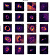Fig. E.1

SPHERE scattered light images. We present the Q_ϕ images that are scaled with r². The gray hatched circles indicate the size of the applied coronagraph. In all frames north points up and east to the left.

References

Akiyama, E., Vorobyov, E. I., Baobabu Liu, H., et al. 2019, AJ, 157, 165 [Google Scholar]
Alcalá, J. M., Manara, C. F., Natta, A., et al. 2017, A&A, 600, A20 [NASA ADS] [CrossRef] [EDP Sciences] [Google Scholar]
Alecian, E., Wade, G. A., Catala, C., et al. 2013, MNRAS, 429, 1001 [NASA ADS] [CrossRef] [Google Scholar]
Alencar, S. H. P., Bouvier, J., Donati, J. F., et al. 2018, A&A, 620, A195 [NASA ADS] [CrossRef] [EDP Sciences] [Google Scholar]
ALMA Partnership (Brogan, C. L., et al.) 2015, ApJ, 808, L3 [Google Scholar]
Andrews, S. M. 2020, ARA&A, 58, 483 [Google Scholar]
Andrews, S. M., Huang, J., Pérez, L. M., et al. 2018, ApJ, 869, L41 [NASA ADS] [CrossRef] [Google Scholar]
Ansdell, M., Williams, J. P., Trapman, L., et al. 2018, ApJ, 859, 21 [NASA ADS] [CrossRef] [Google Scholar]
Ardila, D. R., Golimowski, D. A., Krist, J. E., et al. 2007, ApJ, 665, 512 [Google Scholar]
Asensio-Torres, R., Henning, T., Cantalloube, F., et al. 2021, A&A, 652, A101 [NASA ADS] [CrossRef] [EDP Sciences] [Google Scholar]
Astropy Collaboration (Robitaille, T. P., et al.) 2013, A&A, 558, A33 [NASA ADS] [CrossRef] [EDP Sciences] [Google Scholar]
Astropy Collaboration (Price-Whelan, A. M., et al.) 2018, AJ, 156, 123 [Google Scholar]
Avenhaus, H., Quanz, S. P., Schmid, H. M., et al. 2017, AJ, 154, 33 [Google Scholar]
Avenhaus, H., Quanz, S. P., Garufi, A., et al. 2018, ApJ, 863, 44 [NASA ADS] [CrossRef] [Google Scholar]
Bae, J., Zhu, Z., & Hartmann, L. 2017, ApJ, 850, 201 [NASA ADS] [CrossRef] [Google Scholar]
Bae, J., Zhu, Z., Baruteau, C., et al. 2019, ApJ, 884, L41 [NASA ADS] [CrossRef] [Google Scholar]
Bailer-Jones, C. A. L., Rybizki, J., Fouesneau, M., Demleitner, M., & Andrae, R. 2021, AJ, 161, 147 [Google Scholar]
Ballabio, G., Nealon, R., Alexander, R. D., et al. 2021, MNRAS, 504, 888 [NASA ADS] [CrossRef] [Google Scholar]
Bans, A., & Königl, A. 2012, ApJ, 758, 100 [Google Scholar]
Bate, M. R. 2018, MNRAS, 475, 5618 [Google Scholar]
Bate, M. R., Lodato, G., & Pringle, J. E. 2010, MNRAS, 401, 1505 [NASA ADS] [CrossRef] [Google Scholar]
Benisty, M., Natta, A., Isella, A., et al. 2010, A&A, 511, A74 [NASA ADS] [CrossRef] [EDP Sciences] [Google Scholar]
Benisty, M., Stolker, T., Pohl, A., et al. 2017, A&A, 597, A42 [NASA ADS] [CrossRef] [EDP Sciences] [Google Scholar]
Benisty, M., Juhász, A., Facchini, S., et al. 2018, A&A, 619, A171 [NASA ADS] [CrossRef] [EDP Sciences] [Google Scholar]
Beuzit, J. L., Vigan, A., Mouillet, D., et al. 2019, A&A, 631, A155 [NASA ADS] [CrossRef] [EDP Sciences] [Google Scholar]
Bitsch, B., Crida, A., Libert, A. S., & Lega, E. 2013, A&A, 555, A124 [NASA ADS] [CrossRef] [EDP Sciences] [Google Scholar]
Bodman, E. H. L., Quillen, A. C., Ansdell, M., et al. 2017, MNRAS, 470, 202 [Google Scholar]
Bohn, A. J., Kenworthy, M. A., Ginski, C., et al. 2019, A&A, 624, A87 [EDP Sciences] [Google Scholar]
Bouvier, J., Chelli, A., Allain, S., et al. 1999, A&A, 349, 619 [NASA ADS] [Google Scholar]
Bouvier, J., Grankin, K. N., Alencar, S. H. P., et al. 2003, A&A, 409, 169 [NASA ADS] [CrossRef] [EDP Sciences] [Google Scholar]
Bouvier, J., Perraut, K., Le Bouquin, J. B., et al. 2020, A&A, 636, A108 [NASA ADS] [CrossRef] [EDP Sciences] [Google Scholar]
Bradley, L., Sipocz, B., Robitaille, T., et al. 2016, Photutils: Photometry tools [Google Scholar]
Calvet, N., D’Alessio, P., Hartmann, L., et al. 2002, ApJ, 568, 1008 [Google Scholar]
Cardelli, J. A., Clayton, G. C., & Mathis, J. S. 1989, ApJ, 345, 245 [Google Scholar]
Casassus, S., Avenhaus, H., Pérez, S., et al. 2018, MNRAS, 477, 5104 [NASA ADS] [CrossRef] [Google Scholar]
Chen, L., Moór, A., Kreplin, A., et al. 2019, ApJ, 887, L32 [NASA ADS] [CrossRef] [Google Scholar]
Cody, A. M., & Hillenbrand, L. A. 2018, AJ, 156, 71 [Google Scholar]
Cody, A. M., Stauffer, J., Baglin, A., et al. 2014, AJ, 147, 82 [Google Scholar]
Coulson, I. M., & Walther, D. M. 1995, MNRAS, 274, 977 [NASA ADS] [Google Scholar]
Cutri, R. M., Skrutskie, M. F., van Dyk, S., et al. 2003, VizieR Online Data Catalog: II/246 [Google Scholar]
Davies, C. L. 2019, MNRAS, 484, 1926 [NASA ADS] [CrossRef] [Google Scholar]
Davies, C. L., Kraus, S., Harries, T. J., et al. 2020, ApJ, 897, 31 [NASA ADS] [CrossRef] [Google Scholar]
de Boer, J., Langlois, M., van Holstein, R. G., et al. 2020, A&A, 633, A63 [NASA ADS] [CrossRef] [EDP Sciences] [Google Scholar]
Donati, J. F., Bouvier, J., Alencar, S. H., et al. 2019, MNRAS, 483, L1 [Google Scholar]
Dong, R., van der Marel, N., Hashimoto, J., et al. 2017, ApJ, 836, 201 [NASA ADS] [CrossRef] [Google Scholar]
Duan, Q., Gupta, V. K., & Sorooshian, S. 1993, J. Optim. Theory Appl., 76, 501 [Google Scholar]
Dullemond, C. P., & Monnier, J. D. 2010, ARA&A, 48, 205 [NASA ADS] [CrossRef] [Google Scholar]
Dullemond, C. P., Küffmeier, M., Goicovic, F., et al. 2019, A&A, 628, A20 [NASA ADS] [CrossRef] [EDP Sciences] [Google Scholar]
Espaillat, C., Furlan, E., D’Alessio, P., et al. 2011, ApJ, 728, 49 [NASA ADS] [CrossRef] [Google Scholar]
Espaillat, C., Muzerolle, J., Najita, J., et al. 2014, in Protostars and Planets VI, eds. H. Beuther, R. S. Klessen, C. P. Dullemond, & T. Henning (Tucson: University of Arizona Press), 497 [Google Scholar]
Facchini, S., Lodato, G., & Price, D. J. 2013, MNRAS, 433, 2142 [Google Scholar]
Facchini, S., Juhász, A., & Lodato, G. 2018, MNRAS, 473, 4459 [Google Scholar]
Facchini, S., Benisty, M., Bae, J., et al. 2020, A&A, 639, A121 [EDP Sciences] [Google Scholar]
Fairlamb, J. R., Oudmaijer, R. D., Mendigutía, I., Ilee, J. D., & van den Ancker, M. E. 2015, MNRAS, 453, 976 [Google Scholar]
Feiden, G. A. 2016, A&A, 593, A99 [NASA ADS] [CrossRef] [EDP Sciences] [Google Scholar]
Fekel, F. C., J. 1981, ApJ, 246, 879 [NASA ADS] [CrossRef] [Google Scholar]
Flock, M., Fromang, S., Turner, N. J., & Benisty, M. 2017, ApJ, 835, 230 [CrossRef] [Google Scholar]
Foreman-Mackey, D., Hogg, D. W., Lang, D., & Goodman, J. 2013, PASP, 125, 306 [Google Scholar]
Francis, L., & van der Marel, N. 2020, ApJ, 892, 111 [Google Scholar]
Fukagawa, M., Tamura, M., Itoh, Y., et al. 2006, ApJ, 636, L153 [Google Scholar]
Gahm, G. F., Fischerstrom, C., Liseau, R., & Lindroos, K. P. 1989, A&A, 211, 115 [Google Scholar]
Gaia Collaboration (Brown A. G. A., et al.) 2021, A&A, 649, A1 [NASA ADS] [CrossRef] [EDP Sciences] [Google Scholar]
Garufi, A., Benisty, M., Pinilla, P., et al. 2018, A&A, 620, A94 [NASA ADS] [CrossRef] [EDP Sciences] [Google Scholar]
Ginski, C., Stolker, T., Pinilla, P., et al. 2016, A&A, 595, A112 [NASA ADS] [CrossRef] [EDP Sciences] [Google Scholar]
Ginski, C., Facchini, S., Huang, J., et al. 2021, ApJ, 908, L25 [NASA ADS] [CrossRef] [Google Scholar]
Gonzalez, J.-F., van der Plas, G., Pinte, C., et al. 2020, MNRAS, 499, 3837 [Google Scholar]
GRAVITY Collaboration (Perraut, K., et al.) 2019, A&A, 632, A53 [NASA ADS] [CrossRef] [EDP Sciences] [Google Scholar]
GRAVITY Collaboration (Bouarour, Y. I., et al.) 2020, A&A, 642, A162 [NASA ADS] [CrossRef] [EDP Sciences] [Google Scholar]
GRAVITY Collaboration (Sanchez-Bermudez, J., et al.) 2021, A&A, 654, A97 [NASA ADS] [CrossRef] [EDP Sciences] [Google Scholar]
Grinin, V., Natta, A., & Tambovtseva, L. 1996, A&A, 313, 857 [NASA ADS] [Google Scholar]
Herbig, G. H., Vrba, F. J., & Rydgren, A. E. 1986, AJ, 91, 575 [NASA ADS] [CrossRef] [Google Scholar]
Herbst, W. 2012, J. Am. Assoc. Variab. Star Observ., 40, 448 [NASA ADS] [Google Scholar]
Herbst, W., Herbst, D. K., Grossman, E. J., & Weinstein, D. 1994, AJ, 108, 1906 [Google Scholar]
Herczeg, G. J., & Hillenbrand, L. A. 2014, ApJ, 786, 97 [Google Scholar]
Høg, E., Fabricius, C., Makarov, V. V., et al. 2000, A&A, 355, L27 [Google Scholar]
Huang, J., Andrews, S. M., Dullemond, C. P., et al. 2018, ApJ, 869, L42 [NASA ADS] [CrossRef] [Google Scholar]
Hunter, J. D. 2007, Comput. Sci. Eng., 9, 90 [NASA ADS] [CrossRef] [Google Scholar]
Isella, A., & Natta, A. 2005, A&A, 438, 899 [NASA ADS] [CrossRef] [EDP Sciences] [Google Scholar]
Kama, M., Min, M., & Dominik, C. 2009, A&A, 506, 1199 [NASA ADS] [CrossRef] [EDP Sciences] [Google Scholar]
Keppler, M., Benisty, M., Müller, A., et al. 2018, A&A, 617, A44 [NASA ADS] [CrossRef] [EDP Sciences] [Google Scholar]
Keppler, M., Teague, R., Bae, J., et al. 2019, A&A, 625, A118 [NASA ADS] [CrossRef] [EDP Sciences] [Google Scholar]
Kluska, J., Kraus, S., Davies, C. L., et al. 2018, ApJ, 855, 44 [Google Scholar]
Kraus, S., Ireland, M. J., Sitko, M. L., et al. 2013, ApJ, 768, 80 [NASA ADS] [CrossRef] [Google Scholar]
Kraus, S., Kreplin, A., Fukugawa, M., et al. 2017, ApJ, 848, L11 [Google Scholar]
Kuffmeier, M., Dullemond, C. P., Reissl, S., & Goicovic, F. G. 2021, A&A, 656, A161 [NASA ADS] [CrossRef] [EDP Sciences] [Google Scholar]
Kurosawa, R., & Romanova, M. M. 2013, MNRAS, 431, 2673 [Google Scholar]
Lacour, S., Dembet, R., Abuter, R., et al. 2019, A&A, 624, A99 [NASA ADS] [CrossRef] [EDP Sciences] [Google Scholar]
Langlois, M., Pohl, A., Lagrange, A. M., et al. 2018, A&A, 614, A88 [NASA ADS] [CrossRef] [EDP Sciences] [Google Scholar]
Lapeyrere, V., Kervella, P., Lacour, S., et al. 2014, Proc. SPIE, 9146, 91462D [Google Scholar]
Lazareff, B., Berger, J. P., Kluska, J., et al. 2017, A&A, 599, A85 [NASA ADS] [CrossRef] [EDP Sciences] [Google Scholar]
Loomis, R. A., Öberg, K. I., Andrews, S. M., & MacGregor, M. A. 2017, ApJ, 840, 23 [NASA ADS] [CrossRef] [Google Scholar]
Manara, C. F., Robberto, M., Da Rio, N., et al. 2012, ApJ, 755, 154 [NASA ADS] [CrossRef] [Google Scholar]
Manara, C. F., Testi, L., Natta, A., et al. 2014, A&A, 568, A18 [NASA ADS] [CrossRef] [EDP Sciences] [Google Scholar]
Manset, N., Bastien, P., Ménard, F., et al. 2009, A&A, 499, 137 [NASA ADS] [CrossRef] [EDP Sciences] [Google Scholar]
Marino, S., Perez, S., & Casassus, S. 2015, ApJ, 798, L44 [Google Scholar]
Martin, R. G., Lubow, S. H., Nixon, C., & Armitage, P. J. 2016, MNRAS, 458, 4345 [NASA ADS] [CrossRef] [Google Scholar]
Matsakos, T., & Königl, A. 2017, AJ, 153, 60 [NASA ADS] [CrossRef] [Google Scholar]
McGinnis, P. T., Alencar, S. H. P., Guimarães, M. M., et al. 2015, A&A, 577, A11 [NASA ADS] [CrossRef] [EDP Sciences] [Google Scholar]
Meheut, H., Meliani, Z., Varniere, P., & Benz, W. 2012, A&A, 545, A134 [NASA ADS] [CrossRef] [EDP Sciences] [Google Scholar]
Ménard, F., Cuello, N., Ginski, C., et al. 2020, A&A, 639, L1 [EDP Sciences] [Google Scholar]
Menu, J., van Boekel, R., Henning, T., et al. 2014, A&A, 564, A93 [NASA ADS] [CrossRef] [EDP Sciences] [Google Scholar]
Menu, J., van Boekel, R., Henning, T., et al. 2015, A&A, 581, A107 [NASA ADS] [CrossRef] [EDP Sciences] [Google Scholar]
Min, M., Stolker, T., Dominik, C., & Benisty, M. 2017, A&A, 604, L10 [NASA ADS] [CrossRef] [EDP Sciences] [Google Scholar]
Monet, D. G., Levine, S. E., Canzian, B., et al. 2003, AJ, 125, 984 [Google Scholar]
Monnier, J. D., Millan-Gabet, R., Billmeier, R., et al. 2005, ApJ, 624, 832 [NASA ADS] [CrossRef] [Google Scholar]
Monnier, J. D., Harries, T. J., Aarnio, A., et al. 2017, ApJ, 838, 20 [Google Scholar]
Mora, A., Merín, B., Solano, E., et al. 2001, A&A, 378, 116 [NASA ADS] [CrossRef] [EDP Sciences] [Google Scholar]
Müller, A., Keppler, M., Henning, T., et al. 2018, A&A, 617, L2 [Google Scholar]
Muro-Arena, G. A., Benisty, M., Ginski, C., et al. 2020, A&A, 635, A121 [NASA ADS] [CrossRef] [EDP Sciences] [Google Scholar]
Murphy, S. J., Corbally, C. J., Gray, R. O., et al. 2015, PASA, 32, e036 [Google Scholar]
Natta, A., Prusti, T., Neri, R., et al. 2001, A&A, 371, 186 [NASA ADS] [CrossRef] [EDP Sciences] [Google Scholar]
Nealon, R., Dipierro, G., Alexander, R., Martin, R. G., & Nixon, C. 2018, MNRAS, 481, 20 [Google Scholar]
Nealon, R., Pinte, C., Alexander, R., Mentiplay, D., & Dipierro, G. 2019, MNRAS, 484, 4951 [CrossRef] [Google Scholar]
Nealon, R., Cuello, N., Gonzalez, J.-F., et al. 2020, MNRAS, 499, 3857 [Google Scholar]
Ohta, Y., Fukagawa, M., Sitko, M. L., et al. 2016, PASJ, 68, 53 [Google Scholar]
Oliphant, T. E. 2006, A guide to NumPy (USA: Trelgol Publishing), 1 [Google Scholar]
Owen, J. E., & Lai, D. 2017, MNRAS, 469, 2834 [CrossRef] [Google Scholar]
Pascucci, I., Testi, L., Herczeg, G. J., et al. 2016, ApJ, 831, 125 [Google Scholar]
Pecaut, M. J.,& Mamajek, E. E. 2016, MNRAS, 461, 794 [NASA ADS] [CrossRef] [Google Scholar]
Pedregosa, F., Varoquaux, G., Gramfort, A., et al. 2012, ArXiv e-prints [arXiv:1201.0490] [Google Scholar]
Pérez, L. M., Isella, A., Carpenter, J. M., & Chandler, C. J. 2014, ApJ, 783, L13 [Google Scholar]
Pérez, S., Casassus, S., Hales, A., et al. 2020, ApJ, 889, L24 [Google Scholar]
Pinilla, P., Benisty, M., de Boer, J., et al. 2018, ApJ, 868, 85 [NASA ADS] [CrossRef] [Google Scholar]
Pinte, C., Ménard, F., Berger, J. P., Benisty, M., & Malbet, F. 2008, ApJ, 673, L63 [NASA ADS] [CrossRef] [Google Scholar]
Pinte, C., van der Plas, G., Ménard, F., et al. 2019, Nat. Astron., 3, 1109 [NASA ADS] [CrossRef] [Google Scholar]
Pohl, A., Benisty, M., Pinilla, P., et al. 2017, ApJ, 850, 52 [Google Scholar]
Price, D. J., Cuello, N., Pinte, C., et al. 2018, MNRAS, 477, 1270 [Google Scholar]
Quanz, S. P., Amara, A., Meyer, M. R., et al. 2013, ApJ, 766, L1 [Google Scholar]
Riello, M., De Angeli, F., Evans, D. W., et al. 2021, A&A, 649, A3 [NASA ADS] [CrossRef] [EDP Sciences] [Google Scholar]
Rosotti, G. P., Benisty, M., Juhász, A., et al. 2020, MNRAS, 491, 1335 [Google Scholar]
Sallum, S., Follette, K. B., Eisner, J. A., et al. 2015, Nature, 527, 342 [Google Scholar]
Schmid, H. M., Bazzon, A., Roelfsema, R., et al. 2018, A&A, 619, A9 [NASA ADS] [CrossRef] [EDP Sciences] [Google Scholar]
Setterholm, B. R., Monnier, J. D., Davies, C. L., et al. 2018, ApJ, 869, 164 [NASA ADS] [CrossRef] [Google Scholar]
Sicilia-Aguilar, A., Manara, C. F., de Boer, J., et al. 2020, A&A, 633, A37 [NASA ADS] [CrossRef] [EDP Sciences] [Google Scholar]
Simon, M., Guilloteau, S., Di Folco, E., et al. 2017, ApJ, 844, 158 [Google Scholar]
Skrutskie, M. F., Dutkevitch, D., Strom, S. E., et al. 1990, AJ, 99, 1187 [NASA ADS] [CrossRef] [Google Scholar]
Skrutskie, M. F., Cutri, R. M., Stiening, R., et al. 2006, AJ, 131, 1163 [NASA ADS] [CrossRef] [Google Scholar]
Stolker, T., Dominik, C., Avenhaus, H., et al. 2016, A&A, 595, A113 [NASA ADS] [CrossRef] [EDP Sciences] [Google Scholar]
Stolker, T., Sitko, M., Lazareff, B., et al. 2017, ApJ, 849, 143 [Google Scholar]
Strom, K. M., Strom, S. E., Edwards, S., Cabrit, S., & Skrutskie, M. F. 1989, AJ, 97, 1451 [Google Scholar]
Tannirkulam, A., Monnier, J. D., Harries, T. J., et al. 2008, ApJ, 689, 513 [NASA ADS] [CrossRef] [Google Scholar]
Teague, R. 2019, Res. Notes Am. Astron. Soc., 3, 74 [Google Scholar]
Teague, R., & Foreman-Mackey, D. 2018, Res. Notes Am. Astron. Soc., 2, 173 [Google Scholar]
Teague, R., Bae, J., Bergin, E. A., Birnstiel, T., & Foreman-Mackey, D. 2018, ApJ, 860, L12 [NASA ADS] [CrossRef] [Google Scholar]
Teague, R., Bae, J., & Bergin, E. A. 2019, Nature, 574, 378 [NASA ADS] [CrossRef] [Google Scholar]
Thalmann, C., Janson, M., Garufi, A., et al. 2016, ApJ, 828, L17 [Google Scholar]
Ubeira Gabellini, M. G., Miotello, A., Facchini, S., et al. 2019, MNRAS, 486, 4638 [NASA ADS] [CrossRef] [Google Scholar]
Uyama, T., Currie, T., Christiaens, V., et al. 2020a, ApJ, 900, 135 [NASA ADS] [CrossRef] [Google Scholar]
Uyama, T., Muto, T., Mawet, D., et al. 2020b, AJ, 159, 118 [Google Scholar]
van der Marel,N., van Dishoeck, E. F., Bruderer, S., et al. 2013, Science, 340, 1199 [NASA ADS] [CrossRef] [Google Scholar]
van der Marel,N., van Dishoeck, E. F., Bruderer, S., et al. 2016, A&A, 585, A58 [NASA ADS] [CrossRef] [EDP Sciences] [Google Scholar]
van der Marel,N., Williams, J. P., Ansdell, M., et al. 2018, ApJ, 854, 177 [Google Scholar]
van der Marel,N., Birnstiel, T., Garufi, A., et al. 2021, AJ, 161, 33 [Google Scholar]
Van der Walt, S., Schönberger, J. L., Nunez-Iglesias, J., et al. 2014, PeerJ, 2, e453 [Google Scholar]
van Holstein, R. G., Girard, J. H., de Boer, J., et al. 2020, A&A, 633, A64 [NASA ADS] [CrossRef] [EDP Sciences] [Google Scholar]
van Terwisga, S. E., van Dishoeck, E. F., Cazzoletti, P., et al. 2019, A&A, 623, A150 [NASA ADS] [CrossRef] [EDP Sciences] [Google Scholar]
Varga, J., Hogerheijde, M., van Boekel, R., et al. 2021, A&A, 647, A56 [NASA ADS] [CrossRef] [EDP Sciences] [Google Scholar]
Vieira, S. L. A., Corradi, W. J. B., Alencar, S. H. P., et al. 2003, AJ, 126, 2971 [Google Scholar]
Vioque, M., Oudmaijer, R. D., Baines, D., Mendigutía, I., & Pérez-Martínez, R. 2018, A&A, 620, A128 [NASA ADS] [CrossRef] [EDP Sciences] [Google Scholar]
Virtanen, P., Gommers, R., Oliphant, T. E., et al. 2020, Nat. Methods, 17, 261 [Google Scholar]
Wenger, M., Ochsenbein, F., Egret, D., et al. 2000, A&AS, 143, 9 [NASA ADS] [CrossRef] [EDP Sciences] [Google Scholar]
Wolfer, L., Facchini, S., Kurtovic, N. T., et al. 2021, A&A, 648, A19 [NASA ADS] [CrossRef] [EDP Sciences] [Google Scholar]
Xiang-Gruess, M., & Papaloizou, J. C. B. 2013, MNRAS, 431, 1320 [Google Scholar]
Yu, H., Teague, R., Bae, J., & Öberg, K. 2021, ApJ, 920, L33 [NASA ADS] [CrossRef] [Google Scholar]
Zhu, Z., Nelson, R. P., Hartmann, L., Espaillat, C., & Calvet, N. 2011, ApJ, 729, 47 [NASA ADS] [CrossRef] [Google Scholar]

¹

www.github.com/stijnvanhoey/Optimization_SCE

All Tables

Table 1

Stellar properties of our sample.

In the text

Table 2

Results of our SED fits.

In the text

Table 3

Model parameter and priors of the MCMC fit to the GRAVITY data.

In the text

Table 4

Inner and outer disk geometries of our sample.

In the text

Table A.1

Setup and weather conditions of the GRAVITY observations.

In the text

Table A.2

Basic properties of the ALMA line observations

In the text

Table A.3

Photometric data of the targets in our sample.

In the text

Table B.1

Results of the model fits to the GRAVITY data.

In the text

Table C.1

Results from the outer disk model fits of the ALMA line data cubes.

In the text

All Figures

	Fig. 1 GRAVITY observations and best-fit model for HD 100453. Top left: squared visibilities as a function of spatial frequency. Colors refer to the different baselines. The inset presents the (u, v) plane coverage of the observations. Bottom left: closure phases as a function of the average spatial frequency. The various colors refer to the different triplets. Right panel: best-fit model.
In the text

Fig. 2

SED fit for HD 100453. The circles represent the photometry and the solid purple curve, the best SED model from the MCMC posterior distribution. The model consists of two individual blackbody components that are visualized by the dashed lines: the blue curve represents the stellar flux density whereas the red curve shows the flux density of the circumstellar dust. The dotted line indicates the GRAVITY reference wavelength of 2.25 μm, at which we evaluate the dust flux contribution.

In the text

	Fig. 3 Uncertainties of the inner disk geometric parameters (i_in, PA_in) as a functionof (u, v) plane coverage, C_uv, and the disk half-flux radius, a. The colors indicate the stellar luminosity.
In the text

Fig. 4

Velocity maps and model fits to the ALMA CO line data of HD 100453. In all images north points up and east to the left. Top left: quadratically collapsed moment map derived with bettermoments. Top center: best-fit Keplerian disk model derived with the eddy tool. Top right: residuals after subtraction of the model from the data. Bottom panels: iso-velocity contours of the best-fit model plotted for the individual channel maps of the data cube.

In the text

Fig. 5

Misalignments between inner and outer disks in our sample of transition disks. The upper and bottom panels show the misalignments for the most massive stars of our sample (Herbig Ae/Be and intermediate-mass T Tauri stars) and for the T Tauri stars, respectively. Left panels: comparison of outer and inner disk inclinations. The dashed line indicates perfect alignment in inclination. Right panels: same as left panel but for inner and outer disk position angles. As we do not know the true orientation of the inner disk, we present both possibilities for the inner disk near sides. The full-colored markers represent the position angles from the GRAVITY fits and the white markers with the colored edges have an additional offset of 180°.

In the text

	Fig. 6 KS statistics testing the null hypothesis of perfectly aligned disk geometries. From bottom to top the targets are sorted from best (D_KS = 0) to worst agreement (D_KS = 1) with the null hypothesis. The different shades of background color indicate targets with no significant misalignment (left), significant misalignment (right) and dubious cases in the middle.
In the text

	Fig. 7 Left: scattered light images. Middle, right: same, with predicted lines connecting putative shadows based on both potential misalignment configurations, Δθ₁ and Δθ₂, respectively. The colored lines are 1000 randomly drawn samples from our posterior distributions that describe the shadow locations. The gray circles indicate the coronagraph.
In the text

	Fig. 8 Predicted shadows for ambiguous cases that exhibit shadows in scattered light. The figure elements and image orientations are the same as for Fig. 7.
In the text

	Fig. B.1 Best-fit inner disk models from the GRAVITY observables. In all images north points up and east toward the left.
In the text

Fig. B.2

GRAVITY observables and model fits. In the upper left of each panel, the (u, v) plane coverage is shown. Each symbol corresponds to an individual exposures and the colors refer to the interferometric baselines. The other panels of the plot show the squared visibilities (right) and closure phases (left) for each baseline or triplet as a function of wavelength. The white markers with black contours represent the observational data and the black lines correspond to our best-fit model. The black markers on top of the lines indicate which curve corresponds to which exposure.

In the text

	Fig. C.1 ALMA line data of our targets. We present the quadratically collapsed moment maps that were created with `bettermoments` by quadratic collapsing of the frequency channels. The ellipse in the lower left of each panel indicates the beam size of the observation. For all images north points up and east to the left.
In the text

	Fig. D.1 Posterior distributions of the derived misalignment angles. We also present the simulated distributions for a perfectly aligned disk geometry. Good agreement of the true and simulated distributions indicates that inner and outer disk are well aligned. Deviations from this agreement are signs of potential misalignment.
In the text

	Fig. E.1 SPHERE scattered light images. We present the Q_ϕ images that are scaled with r². The gray hatched circles indicate the size of the applied coronagraph. In all frames north points up and east to the left.
In the text

Current usage metrics show cumulative count of Article Views (full-text article views including HTML views, PDF and ePub downloads, according to the available data) and Abstracts Views on Vision4Press platform.

Data correspond to usage on the plateform after 2015. The current usage metrics is available 48-96 hours after online publication and is updated daily on week days.

Initial download of the metrics may take a while.

[1] Akiyama, E., Vorobyov, E. I., Baobabu Liu, H., et al. 2019, AJ, 157, 165 [Google Scholar]

[2] Alcalá, J. M., Manara, C. F., Natta, A., et al. 2017, A&A, 600, A20 [NASA ADS] [CrossRef] [EDP Sciences] [Google Scholar]

[3] Alecian, E., Wade, G. A., Catala, C., et al. 2013, MNRAS, 429, 1001 [NASA ADS] [CrossRef] [Google Scholar]

[4] Alencar, S. H. P., Bouvier, J., Donati, J. F., et al. 2018, A&A, 620, A195 [NASA ADS] [CrossRef] [EDP Sciences] [Google Scholar]

[5] ALMA Partnership (Brogan, C. L., et al.) 2015, ApJ, 808, L3 [Google Scholar]

[6] Andrews, S. M. 2020, ARA&A, 58, 483 [Google Scholar]

[7] Andrews, S. M., Huang, J., Pérez, L. M., et al. 2018, ApJ, 869, L41 [NASA ADS] [CrossRef] [Google Scholar]

[8] Ansdell, M., Williams, J. P., Trapman, L., et al. 2018, ApJ, 859, 21 [NASA ADS] [CrossRef] [Google Scholar]

[9] Ardila, D. R., Golimowski, D. A., Krist, J. E., et al. 2007, ApJ, 665, 512 [Google Scholar]

[10] Asensio-Torres, R., Henning, T., Cantalloube, F., et al. 2021, A&A, 652, A101 [NASA ADS] [CrossRef] [EDP Sciences] [Google Scholar]

[11] Astropy Collaboration (Robitaille, T. P., et al.) 2013, A&A, 558, A33 [NASA ADS] [CrossRef] [EDP Sciences] [Google Scholar]

[12] Astropy Collaboration (Price-Whelan, A. M., et al.) 2018, AJ, 156, 123 [Google Scholar]

[13] Avenhaus, H., Quanz, S. P., Schmid, H. M., et al. 2017, AJ, 154, 33 [Google Scholar]

[14] Avenhaus, H., Quanz, S. P., Garufi, A., et al. 2018, ApJ, 863, 44 [NASA ADS] [CrossRef] [Google Scholar]

[15] Bae, J., Zhu, Z., & Hartmann, L. 2017, ApJ, 850, 201 [NASA ADS] [CrossRef] [Google Scholar]

[16] Bae, J., Zhu, Z., Baruteau, C., et al. 2019, ApJ, 884, L41 [NASA ADS] [CrossRef] [Google Scholar]

[17] Bailer-Jones, C. A. L., Rybizki, J., Fouesneau, M., Demleitner, M., & Andrae, R. 2021, AJ, 161, 147 [Google Scholar]

[18] Ballabio, G., Nealon, R., Alexander, R. D., et al. 2021, MNRAS, 504, 888 [NASA ADS] [CrossRef] [Google Scholar]

[19] Bans, A., & Königl, A. 2012, ApJ, 758, 100 [Google Scholar]

[20] Bate, M. R. 2018, MNRAS, 475, 5618 [Google Scholar]

[21] Bate, M. R., Lodato, G., & Pringle, J. E. 2010, MNRAS, 401, 1505 [NASA ADS] [CrossRef] [Google Scholar]

[22] Benisty, M., Natta, A., Isella, A., et al. 2010, A&A, 511, A74 [NASA ADS] [CrossRef] [EDP Sciences] [Google Scholar]

[23] Benisty, M., Stolker, T., Pohl, A., et al. 2017, A&A, 597, A42 [NASA ADS] [CrossRef] [EDP Sciences] [Google Scholar]

[24] Benisty, M., Juhász, A., Facchini, S., et al. 2018, A&A, 619, A171 [NASA ADS] [CrossRef] [EDP Sciences] [Google Scholar]

[25] Beuzit, J. L., Vigan, A., Mouillet, D., et al. 2019, A&A, 631, A155 [NASA ADS] [CrossRef] [EDP Sciences] [Google Scholar]

[26] Bitsch, B., Crida, A., Libert, A. S., & Lega, E. 2013, A&A, 555, A124 [NASA ADS] [CrossRef] [EDP Sciences] [Google Scholar]

[27] Bodman, E. H. L., Quillen, A. C., Ansdell, M., et al. 2017, MNRAS, 470, 202 [Google Scholar]

[28] Bohn, A. J., Kenworthy, M. A., Ginski, C., et al. 2019, A&A, 624, A87 [EDP Sciences] [Google Scholar]

[29] Bouvier, J., Chelli, A., Allain, S., et al. 1999, A&A, 349, 619 [NASA ADS] [Google Scholar]

[30] Bouvier, J., Grankin, K. N., Alencar, S. H. P., et al. 2003, A&A, 409, 169 [NASA ADS] [CrossRef] [EDP Sciences] [Google Scholar]

[31] Bouvier, J., Perraut, K., Le Bouquin, J. B., et al. 2020, A&A, 636, A108 [NASA ADS] [CrossRef] [EDP Sciences] [Google Scholar]

[32] Bradley, L., Sipocz, B., Robitaille, T., et al. 2016, Photutils: Photometry tools [Google Scholar]

[33] Calvet, N., D’Alessio, P., Hartmann, L., et al. 2002, ApJ, 568, 1008 [Google Scholar]

[34] Cardelli, J. A., Clayton, G. C., & Mathis, J. S. 1989, ApJ, 345, 245 [Google Scholar]

[35] Casassus, S., Avenhaus, H., Pérez, S., et al. 2018, MNRAS, 477, 5104 [NASA ADS] [CrossRef] [Google Scholar]

[36] Chen, L., Moór, A., Kreplin, A., et al. 2019, ApJ, 887, L32 [NASA ADS] [CrossRef] [Google Scholar]

[37] Cody, A. M., & Hillenbrand, L. A. 2018, AJ, 156, 71 [Google Scholar]

[38] Cody, A. M., Stauffer, J., Baglin, A., et al. 2014, AJ, 147, 82 [Google Scholar]

[39] Coulson, I. M., & Walther, D. M. 1995, MNRAS, 274, 977 [NASA ADS] [Google Scholar]

[40] Cutri, R. M., Skrutskie, M. F., van Dyk, S., et al. 2003, VizieR Online Data Catalog: II/246 [Google Scholar]

[41] Davies, C. L. 2019, MNRAS, 484, 1926 [NASA ADS] [CrossRef] [Google Scholar]

[42] Davies, C. L., Kraus, S., Harries, T. J., et al. 2020, ApJ, 897, 31 [NASA ADS] [CrossRef] [Google Scholar]

[43] de Boer, J., Langlois, M., van Holstein, R. G., et al. 2020, A&A, 633, A63 [NASA ADS] [CrossRef] [EDP Sciences] [Google Scholar]

[44] Donati, J. F., Bouvier, J., Alencar, S. H., et al. 2019, MNRAS, 483, L1 [Google Scholar]

[45] Dong, R., van der Marel, N., Hashimoto, J., et al. 2017, ApJ, 836, 201 [NASA ADS] [CrossRef] [Google Scholar]

[46] Duan, Q., Gupta, V. K., & Sorooshian, S. 1993, J. Optim. Theory Appl., 76, 501 [Google Scholar]

[47] Dullemond, C. P., & Monnier, J. D. 2010, ARA&A, 48, 205 [NASA ADS] [CrossRef] [Google Scholar]

[48] Dullemond, C. P., Küffmeier, M., Goicovic, F., et al. 2019, A&A, 628, A20 [NASA ADS] [CrossRef] [EDP Sciences] [Google Scholar]

[49] Espaillat, C., Furlan, E., D’Alessio, P., et al. 2011, ApJ, 728, 49 [NASA ADS] [CrossRef] [Google Scholar]

[50] Espaillat, C., Muzerolle, J., Najita, J., et al. 2014, in Protostars and Planets VI, eds. H. Beuther, R. S. Klessen, C. P. Dullemond, & T. Henning (Tucson: University of Arizona Press), 497 [Google Scholar]

[51] Facchini, S., Lodato, G., & Price, D. J. 2013, MNRAS, 433, 2142 [Google Scholar]

[52] Facchini, S., Juhász, A., & Lodato, G. 2018, MNRAS, 473, 4459 [Google Scholar]

[53] Facchini, S., Benisty, M., Bae, J., et al. 2020, A&A, 639, A121 [EDP Sciences] [Google Scholar]

[54] Fairlamb, J. R., Oudmaijer, R. D., Mendigutía, I., Ilee, J. D., & van den Ancker, M. E. 2015, MNRAS, 453, 976 [Google Scholar]

[55] Feiden, G. A. 2016, A&A, 593, A99 [NASA ADS] [CrossRef] [EDP Sciences] [Google Scholar]

[56] Fekel, F. C., J. 1981, ApJ, 246, 879 [NASA ADS] [CrossRef] [Google Scholar]

[57] Flock, M., Fromang, S., Turner, N. J., & Benisty, M. 2017, ApJ, 835, 230 [CrossRef] [Google Scholar]

[58] Foreman-Mackey, D., Hogg, D. W., Lang, D., & Goodman, J. 2013, PASP, 125, 306 [Google Scholar]

[59] Francis, L., & van der Marel, N. 2020, ApJ, 892, 111 [Google Scholar]

[60] Fukagawa, M., Tamura, M., Itoh, Y., et al. 2006, ApJ, 636, L153 [Google Scholar]

[61] Gahm, G. F., Fischerstrom, C., Liseau, R., & Lindroos, K. P. 1989, A&A, 211, 115 [Google Scholar]

[62] Gaia Collaboration (Brown A. G. A., et al.) 2021, A&A, 649, A1 [NASA ADS] [CrossRef] [EDP Sciences] [Google Scholar]

[63] Garufi, A., Benisty, M., Pinilla, P., et al. 2018, A&A, 620, A94 [NASA ADS] [CrossRef] [EDP Sciences] [Google Scholar]

[64] Ginski, C., Stolker, T., Pinilla, P., et al. 2016, A&A, 595, A112 [NASA ADS] [CrossRef] [EDP Sciences] [Google Scholar]

[65] Ginski, C., Facchini, S., Huang, J., et al. 2021, ApJ, 908, L25 [NASA ADS] [CrossRef] [Google Scholar]

[66] Gonzalez, J.-F., van der Plas, G., Pinte, C., et al. 2020, MNRAS, 499, 3837 [Google Scholar]

[67] GRAVITY Collaboration (Perraut, K., et al.) 2019, A&A, 632, A53 [NASA ADS] [CrossRef] [EDP Sciences] [Google Scholar]

[68] GRAVITY Collaboration (Bouarour, Y. I., et al.) 2020, A&A, 642, A162 [NASA ADS] [CrossRef] [EDP Sciences] [Google Scholar]

[69] GRAVITY Collaboration (Sanchez-Bermudez, J., et al.) 2021, A&A, 654, A97 [NASA ADS] [CrossRef] [EDP Sciences] [Google Scholar]

[70] Grinin, V., Natta, A., & Tambovtseva, L. 1996, A&A, 313, 857 [NASA ADS] [Google Scholar]

[71] Herbig, G. H., Vrba, F. J., & Rydgren, A. E. 1986, AJ, 91, 575 [NASA ADS] [CrossRef] [Google Scholar]

[72] Herbst, W. 2012, J. Am. Assoc. Variab. Star Observ., 40, 448 [NASA ADS] [Google Scholar]

[73] Herbst, W., Herbst, D. K., Grossman, E. J., & Weinstein, D. 1994, AJ, 108, 1906 [Google Scholar]

[74] Herczeg, G. J., & Hillenbrand, L. A. 2014, ApJ, 786, 97 [Google Scholar]

[75] Høg, E., Fabricius, C., Makarov, V. V., et al. 2000, A&A, 355, L27 [Google Scholar]

[76] Huang, J., Andrews, S. M., Dullemond, C. P., et al. 2018, ApJ, 869, L42 [NASA ADS] [CrossRef] [Google Scholar]

[77] Hunter, J. D. 2007, Comput. Sci. Eng., 9, 90 [NASA ADS] [CrossRef] [Google Scholar]

[78] Isella, A., & Natta, A. 2005, A&A, 438, 899 [NASA ADS] [CrossRef] [EDP Sciences] [Google Scholar]

[79] Kama, M., Min, M., & Dominik, C. 2009, A&A, 506, 1199 [NASA ADS] [CrossRef] [EDP Sciences] [Google Scholar]

[80] Keppler, M., Benisty, M., Müller, A., et al. 2018, A&A, 617, A44 [NASA ADS] [CrossRef] [EDP Sciences] [Google Scholar]

[81] Keppler, M., Teague, R., Bae, J., et al. 2019, A&A, 625, A118 [NASA ADS] [CrossRef] [EDP Sciences] [Google Scholar]

[82] Kluska, J., Kraus, S., Davies, C. L., et al. 2018, ApJ, 855, 44 [Google Scholar]

[83] Kraus, S., Ireland, M. J., Sitko, M. L., et al. 2013, ApJ, 768, 80 [NASA ADS] [CrossRef] [Google Scholar]

[84] Kraus, S., Kreplin, A., Fukugawa, M., et al. 2017, ApJ, 848, L11 [Google Scholar]

[85] Kuffmeier, M., Dullemond, C. P., Reissl, S., & Goicovic, F. G. 2021, A&A, 656, A161 [NASA ADS] [CrossRef] [EDP Sciences] [Google Scholar]

[86] Kurosawa, R., & Romanova, M. M. 2013, MNRAS, 431, 2673 [Google Scholar]

[87] Lacour, S., Dembet, R., Abuter, R., et al. 2019, A&A, 624, A99 [NASA ADS] [CrossRef] [EDP Sciences] [Google Scholar]

[88] Langlois, M., Pohl, A., Lagrange, A. M., et al. 2018, A&A, 614, A88 [NASA ADS] [CrossRef] [EDP Sciences] [Google Scholar]

[89] Lapeyrere, V., Kervella, P., Lacour, S., et al. 2014, Proc. SPIE, 9146, 91462D [Google Scholar]

[90] Lazareff, B., Berger, J. P., Kluska, J., et al. 2017, A&A, 599, A85 [NASA ADS] [CrossRef] [EDP Sciences] [Google Scholar]

[91] Loomis, R. A., Öberg, K. I., Andrews, S. M., & MacGregor, M. A. 2017, ApJ, 840, 23 [NASA ADS] [CrossRef] [Google Scholar]

[92] Manara, C. F., Robberto, M., Da Rio, N., et al. 2012, ApJ, 755, 154 [NASA ADS] [CrossRef] [Google Scholar]

[93] Manara, C. F., Testi, L., Natta, A., et al. 2014, A&A, 568, A18 [NASA ADS] [CrossRef] [EDP Sciences] [Google Scholar]

[94] Manset, N., Bastien, P., Ménard, F., et al. 2009, A&A, 499, 137 [NASA ADS] [CrossRef] [EDP Sciences] [Google Scholar]

[95] Marino, S., Perez, S., & Casassus, S. 2015, ApJ, 798, L44 [Google Scholar]

[96] Martin, R. G., Lubow, S. H., Nixon, C., & Armitage, P. J. 2016, MNRAS, 458, 4345 [NASA ADS] [CrossRef] [Google Scholar]

[97] Matsakos, T., & Königl, A. 2017, AJ, 153, 60 [NASA ADS] [CrossRef] [Google Scholar]

[98] McGinnis, P. T., Alencar, S. H. P., Guimarães, M. M., et al. 2015, A&A, 577, A11 [NASA ADS] [CrossRef] [EDP Sciences] [Google Scholar]

[99] Meheut, H., Meliani, Z., Varniere, P., & Benz, W. 2012, A&A, 545, A134 [NASA ADS] [CrossRef] [EDP Sciences] [Google Scholar]

[100] Ménard, F., Cuello, N., Ginski, C., et al. 2020, A&A, 639, L1 [EDP Sciences] [Google Scholar]

[101] Menu, J., van Boekel, R., Henning, T., et al. 2014, A&A, 564, A93 [NASA ADS] [CrossRef] [EDP Sciences] [Google Scholar]

[102] Menu, J., van Boekel, R., Henning, T., et al. 2015, A&A, 581, A107 [NASA ADS] [CrossRef] [EDP Sciences] [Google Scholar]

[103] Min, M., Stolker, T., Dominik, C., & Benisty, M. 2017, A&A, 604, L10 [NASA ADS] [CrossRef] [EDP Sciences] [Google Scholar]

[104] Monet, D. G., Levine, S. E., Canzian, B., et al. 2003, AJ, 125, 984 [Google Scholar]

[105] Monnier, J. D., Millan-Gabet, R., Billmeier, R., et al. 2005, ApJ, 624, 832 [NASA ADS] [CrossRef] [Google Scholar]

[106] Monnier, J. D., Harries, T. J., Aarnio, A., et al. 2017, ApJ, 838, 20 [Google Scholar]

[107] Mora, A., Merín, B., Solano, E., et al. 2001, A&A, 378, 116 [NASA ADS] [CrossRef] [EDP Sciences] [Google Scholar]

[108] Müller, A., Keppler, M., Henning, T., et al. 2018, A&A, 617, L2 [Google Scholar]

[109] Muro-Arena, G. A., Benisty, M., Ginski, C., et al. 2020, A&A, 635, A121 [NASA ADS] [CrossRef] [EDP Sciences] [Google Scholar]

[110] Murphy, S. J., Corbally, C. J., Gray, R. O., et al. 2015, PASA, 32, e036 [Google Scholar]

[111] Natta, A., Prusti, T., Neri, R., et al. 2001, A&A, 371, 186 [NASA ADS] [CrossRef] [EDP Sciences] [Google Scholar]

[112] Nealon, R., Dipierro, G., Alexander, R., Martin, R. G., & Nixon, C. 2018, MNRAS, 481, 20 [Google Scholar]

[113] Nealon, R., Pinte, C., Alexander, R., Mentiplay, D., & Dipierro, G. 2019, MNRAS, 484, 4951 [CrossRef] [Google Scholar]

[114] Nealon, R., Cuello, N., Gonzalez, J.-F., et al. 2020, MNRAS, 499, 3857 [Google Scholar]

[115] Ohta, Y., Fukagawa, M., Sitko, M. L., et al. 2016, PASJ, 68, 53 [Google Scholar]

[116] Oliphant, T. E. 2006, A guide to NumPy (USA: Trelgol Publishing), 1 [Google Scholar]

[117] Owen, J. E., & Lai, D. 2017, MNRAS, 469, 2834 [CrossRef] [Google Scholar]

[118] Pascucci, I., Testi, L., Herczeg, G. J., et al. 2016, ApJ, 831, 125 [Google Scholar]

[119] Pecaut, M. J.,& Mamajek, E. E. 2016, MNRAS, 461, 794 [NASA ADS] [CrossRef] [Google Scholar]

[120] Pedregosa, F., Varoquaux, G., Gramfort, A., et al. 2012, ArXiv e-prints [arXiv:1201.0490] [Google Scholar]

[121] Pérez, L. M., Isella, A., Carpenter, J. M., & Chandler, C. J. 2014, ApJ, 783, L13 [Google Scholar]

[122] Pérez, S., Casassus, S., Hales, A., et al. 2020, ApJ, 889, L24 [Google Scholar]

[123] Pinilla, P., Benisty, M., de Boer, J., et al. 2018, ApJ, 868, 85 [NASA ADS] [CrossRef] [Google Scholar]

[124] Pinte, C., Ménard, F., Berger, J. P., Benisty, M., & Malbet, F. 2008, ApJ, 673, L63 [NASA ADS] [CrossRef] [Google Scholar]

[125] Pinte, C., van der Plas, G., Ménard, F., et al. 2019, Nat. Astron., 3, 1109 [NASA ADS] [CrossRef] [Google Scholar]

[126] Pohl, A., Benisty, M., Pinilla, P., et al. 2017, ApJ, 850, 52 [Google Scholar]

[127] Price, D. J., Cuello, N., Pinte, C., et al. 2018, MNRAS, 477, 1270 [Google Scholar]

[128] Quanz, S. P., Amara, A., Meyer, M. R., et al. 2013, ApJ, 766, L1 [Google Scholar]

[129] Riello, M., De Angeli, F., Evans, D. W., et al. 2021, A&A, 649, A3 [NASA ADS] [CrossRef] [EDP Sciences] [Google Scholar]

[130] Rosotti, G. P., Benisty, M., Juhász, A., et al. 2020, MNRAS, 491, 1335 [Google Scholar]

[131] Sallum, S., Follette, K. B., Eisner, J. A., et al. 2015, Nature, 527, 342 [Google Scholar]

[132] Schmid, H. M., Bazzon, A., Roelfsema, R., et al. 2018, A&A, 619, A9 [NASA ADS] [CrossRef] [EDP Sciences] [Google Scholar]

[133] Setterholm, B. R., Monnier, J. D., Davies, C. L., et al. 2018, ApJ, 869, 164 [NASA ADS] [CrossRef] [Google Scholar]

[134] Sicilia-Aguilar, A., Manara, C. F., de Boer, J., et al. 2020, A&A, 633, A37 [NASA ADS] [CrossRef] [EDP Sciences] [Google Scholar]

[135] Simon, M., Guilloteau, S., Di Folco, E., et al. 2017, ApJ, 844, 158 [Google Scholar]

[136] Skrutskie, M. F., Dutkevitch, D., Strom, S. E., et al. 1990, AJ, 99, 1187 [NASA ADS] [CrossRef] [Google Scholar]

[137] Skrutskie, M. F., Cutri, R. M., Stiening, R., et al. 2006, AJ, 131, 1163 [NASA ADS] [CrossRef] [Google Scholar]

[138] Stolker, T., Dominik, C., Avenhaus, H., et al. 2016, A&A, 595, A113 [NASA ADS] [CrossRef] [EDP Sciences] [Google Scholar]

[139] Stolker, T., Sitko, M., Lazareff, B., et al. 2017, ApJ, 849, 143 [Google Scholar]

[140] Strom, K. M., Strom, S. E., Edwards, S., Cabrit, S., & Skrutskie, M. F. 1989, AJ, 97, 1451 [Google Scholar]

[141] Tannirkulam, A., Monnier, J. D., Harries, T. J., et al. 2008, ApJ, 689, 513 [NASA ADS] [CrossRef] [Google Scholar]

[142] Teague, R. 2019, Res. Notes Am. Astron. Soc., 3, 74 [Google Scholar]

[143] Teague, R., & Foreman-Mackey, D. 2018, Res. Notes Am. Astron. Soc., 2, 173 [Google Scholar]

[144] Teague, R., Bae, J., Bergin, E. A., Birnstiel, T., & Foreman-Mackey, D. 2018, ApJ, 860, L12 [NASA ADS] [CrossRef] [Google Scholar]

[145] Teague, R., Bae, J., & Bergin, E. A. 2019, Nature, 574, 378 [NASA ADS] [CrossRef] [Google Scholar]

[146] Thalmann, C., Janson, M., Garufi, A., et al. 2016, ApJ, 828, L17 [Google Scholar]

[147] Ubeira Gabellini, M. G., Miotello, A., Facchini, S., et al. 2019, MNRAS, 486, 4638 [NASA ADS] [CrossRef] [Google Scholar]

[148] Uyama, T., Currie, T., Christiaens, V., et al. 2020a, ApJ, 900, 135 [NASA ADS] [CrossRef] [Google Scholar]

[149] Uyama, T., Muto, T., Mawet, D., et al. 2020b, AJ, 159, 118 [Google Scholar]

[150] van der Marel,N., van Dishoeck, E. F., Bruderer, S., et al. 2013, Science, 340, 1199 [NASA ADS] [CrossRef] [Google Scholar]

[151] van der Marel,N., van Dishoeck, E. F., Bruderer, S., et al. 2016, A&A, 585, A58 [NASA ADS] [CrossRef] [EDP Sciences] [Google Scholar]

[152] van der Marel,N., Williams, J. P., Ansdell, M., et al. 2018, ApJ, 854, 177 [Google Scholar]

[153] van der Marel,N., Birnstiel, T., Garufi, A., et al. 2021, AJ, 161, 33 [Google Scholar]

[154] Van der Walt, S., Schönberger, J. L., Nunez-Iglesias, J., et al. 2014, PeerJ, 2, e453 [Google Scholar]

[155] van Holstein, R. G., Girard, J. H., de Boer, J., et al. 2020, A&A, 633, A64 [NASA ADS] [CrossRef] [EDP Sciences] [Google Scholar]

[156] van Terwisga, S. E., van Dishoeck, E. F., Cazzoletti, P., et al. 2019, A&A, 623, A150 [NASA ADS] [CrossRef] [EDP Sciences] [Google Scholar]

[157] Varga, J., Hogerheijde, M., van Boekel, R., et al. 2021, A&A, 647, A56 [NASA ADS] [CrossRef] [EDP Sciences] [Google Scholar]

[158] Vieira, S. L. A., Corradi, W. J. B., Alencar, S. H. P., et al. 2003, AJ, 126, 2971 [Google Scholar]

[159] Vioque, M., Oudmaijer, R. D., Baines, D., Mendigutía, I., & Pérez-Martínez, R. 2018, A&A, 620, A128 [NASA ADS] [CrossRef] [EDP Sciences] [Google Scholar]

[160] Virtanen, P., Gommers, R., Oliphant, T. E., et al. 2020, Nat. Methods, 17, 261 [Google Scholar]

[161] Wenger, M., Ochsenbein, F., Egret, D., et al. 2000, A&AS, 143, 9 [NASA ADS] [CrossRef] [EDP Sciences] [Google Scholar]

[162] Wolfer, L., Facchini, S., Kurtovic, N. T., et al. 2021, A&A, 648, A19 [NASA ADS] [CrossRef] [EDP Sciences] [Google Scholar]