| Issue |
A&A
Volume 658, February 2022
|
|
|---|---|---|
| Article Number | A169 | |
| Number of page(s) | 22 | |
| Section | Stellar atmospheres | |
| DOI | https://doi.org/10.1051/0004-6361/202142037 | |
| Published online | 21 February 2022 | |
The super-soft source phase of the recurrent nova V3890 Sgr
1
European Space Agency (ESA), European Space Astronomy Centre (ESAC), Camino Bajo del Castillo s/n,
28692
Villanueva de la Cañada,
Madrid,
Spain
e-mail: This email address is being protected from spambots. You need JavaScript enabled to view it.
2
School of Physics & Astronomy, University of Leicester,
Leicester,
LE1 7RH,
UK
3
Advanced Technologies Research Institute, Faculty of Materials Science and Technology in Trnava, Slovak University of Technology in Bratislava,
Bottova 25,
917 24
Trnava,
Slovakia
4
Harvard-Smithsonian Center for Astrophysics,
60 Garden Street,
Cambridge,
MA
02138,
USA
5
Sterrenkundig Observatorium, Ghent University,
Krijgslaan 281 - S9,
9000
Gent,
Belgium
6
Department of Astronomy, University of Wisconsin,
475 N, Charter Str.,
Madison,
WI
53706,
USA
7
INAF – Osservatorio di Padova,
Vicolo Osservatorio 5,
35122
Padova,
Italy
8
INAF – IASF Palermo,
Via U. La Malfa 153,
90146
Palermo,
Italy
9
Indian institute of Science Education and Research Mohali,
Sector 81, SAS Nagar,
Manauli
PO 140306,
India
10
School of Earth and Space Exploration, Arizona State University,
Tempe,
AZ
85287-1404,
USA
Received:
17
August
2021
Accepted:
30
October
2021
Abstract
Context. The 30-yr recurrent symbiotic nova V3890 Sgr exploded on 2019 August 28 and was observed with multiple X-ray telescopes. Swift and AstroSat monitoring revealed slowly declining hard X-ray emission from shocks between the nova ejecta and the stellar wind of the companion. Later, highly variable super-soft-source (SSS) emission was seen. An XMM-Newton observation during the SSS phase captured the high degree of X-ray variability in terms of a deep dip in the middle of the observation.
Aims. This observation adds to the growing sample of diverse SSS spectra and allows spectral comparison of low- and high-state emission to identify the origin of variations and subsequent effects of such dips, all leading to new insights into how the nova ejecta evolve.
Methods. Based on an initial visual inspection, quantitative modelling approaches were conceptualised to test hypotheses of interpretation. The light curve was analysed with a power spectrum analysis before and after the dip and with an eclipse model to test the hypothesis of occulting clumps as in U Sco. A phenomenological spectral model (SPEX) was used to fit the complex Reflection Grating Spectrometer (RGS) spectrum accounting for all known atomic physics. A blackbody source function was assumed, as in all atmosphere radiation transport models, while the complex radiation transport processes were not modelled. Instead, one or multiple absorbing layers were used to model the absorption lines and edges, taking into account all state-of-the-art knowledge of atomic physics.
Results. In addition to the central deep dip, there is an initial rise of similar depth and shape, and, after the deep dip, there are smaller dips of ~10% amplitude, which might be periodic over 18.1-min. Our eclipse model of the dips yields clump sizes and orbital radii of 0.5–8 and 5–150 white dwarf radii, respectively. The simultaneous XMM-Newton UV light curve shows no significant variations beyond slow fading. The RGS spectrum contains both residual shock emission at short wavelengths and the SSS emission at longer wavelengths. The shock temperature has clearly decreased compared to an earlier Chandra observation (day 6). The dip spectrum is dominated by emission lines as in U Sco. The intensity of underlying blackbody-like emission is much lower with the blackbody normalisation yielding a similar radius to that of the brighter phases, while the lower bolometric luminosity is ascribed to lower Teff. This would be inconsistent with clump occultations unless Compton scattering of the continuum emission reduces the photon energies to mimic a lower effective temperature. However, systematic uncertainties are high. The absorption lines in the bright SSS spectrum are blueshifted by 870 ± 10 km s−1 before the dip and are slightly faster, 900 ± 10 km s−1, after the dip. The reproduction of the observed spectrum is astonishing, especially that only a single absorbing layer is necessary while three such layers are needed to reproduce the RGS spectrum of V2491 Cyg. The ejecta of V3890 Sgr are thus more homogeneous than many other SSS spectra indicate. Abundance determination is in principle possible but highly uncertain. Generally, solar abundances are found, except for N and possibly O, which are higher by an order of magnitude.
Conclusions. High-amplitude variability of SSS emission can be explained in several ways without having to give up the concept of constant bolometric luminosity. Variations in the photospheric radius can expose deeper lying plasma that could pulse with 18.1 min and that would yield a higher outflow velocity. Also, clump occultations are consistent with the observations.
Key words: novae, cataclysmic variables / X-rays: binaries
© ESO 2022
1 Introduction
While there is a high degree of diversity among stars, binaries are even more diverse, not only because of all the types of combinations of different stars, but also the various types of interactions between the two binary components. The class of cataclysmic variables (CVs) is defined by a white dwarf (WD) primary that accretes material from a secondary star. Properties of the WD that drive the observable characteristics are its mass, magnetic fields, and, to a lesser degree, parameters such as its spin period and surface composition. Accreting WDs with low magnetic fields are surrounded by an accretion disc, while those with strong magnetic fields, known as polars, accrete directly towards the magnetic poles. The properties of the companion star determine the properties of the accreted material, whereas the properties of the orbit (e.g. binary separation) drive parameters such as the accretion rate.
The class of symbiotic binaries is characterised by an evolved secondary star revolving around a WD primary in a wide (years) orbit. Evolved stars contribute a dense stellar wind with the capacity to absorb significant amounts of kinetic energy via shocks. While close CV binaries accrete via an overflow of material from the companion star through the Lagrange point 1 (L1), the companion star may not fill its Roche Lobe in a wide binary system. However, the high density of the stellar wind of an evolved star can still facilitate a significant accretion rate (wind accretor).
The class of novae are those CVs that accumulate hydrogen-rich accreted material on the surface of the white dwarf until the pressure is high enough to ignite explosive thermo-nuclear runaway reactions. The energy produced by CNO cycle nuclear fusion of hydrogen to helium is initially released as high-energy radiation that couples with the surface material, which is then ejected via radiation pressure. The ejected shell around the WD is optically thick to high-energy radiation, which is reprocessed to escape at optical and UV wavelengths through a photosphere (with variable radius) after undergoing complex radiation transport processes. Since the ejecta are not in hydrostatic equilibrium, the photospheric radius shrinks with time as the density of the outer ejecta decreases with the continuing expansion. This allows successively deeper views into the outflow, and Teff thus increases with time. Effectively, a nova is bright in optical light during the early evolutionary phases, and, while it declines in the optical, it becomes brighter in the UV bands. As long as the central nuclear burning rate remains stable, Lbol will not change when the peak of the spectral energy distribution gradually shifts to higher energies. With the continued outflow, the density of the outer ejecta goes down, becoming transparent. Eventually, the photospheric radius shrinks to near the surface of the white dwarf, and the observable spectrum then peaks in the soft X-rays (e.g. Starrfield et al. 2008). Most of the soft X-rays are absorbed in the interstellar medium with typical values of neutral hydrogen column densities several 1021 cm−2. The spectrum observed from Earth is known as the class of super-soft sources (SSS).
A nova is called recurrent if more than one outburst has been observed, obviously leading to a bias of novae with recurrence timescales of <100 yr. Since the white dwarf is not destroyed during the outburst and the binary orbit is not significantly altered, all novae should be recurrent. Recurrence timescales depend on the accretion rate (which drives how quickly fuel can be accumulated) and the WD mass (which drives the ignition conditions that are easy or difficult to achieve). For example, a higher WD mass already allows ignition at a lower amount of accreted mass.
V3890 Sgr is a recurrent (~30 yr) nova in a symbiotic binary system and has a famous sibling of the same type, RS Oph (~ 20 yr; see e.g. Ness et al. 2007). The ejecta from the nova outburst run into the dense wind of the evolved companion star where they dissipate some of their kinetic energy in the form of shocks, which is then released as radiation in the X-ray band consisting of bremsstrahlung continuum and characteristic collisionally excited emission lines that originate from collisionally ionised plasma.
The distance to V3890 Sgr can be assumed to be of the order of 9 kpc (Mikołajewska et al. 2021). Depending on the method, smaller values have been derived, for example 4.5 kpc from equivalent widths of the interstellar lines or 4.3 kpc from Gaia DR2. However, Mikołajewska et al. (2021) argue that it is not helpful that the Gaia EDR3 parallax is much different from the DR2 value. Also, Schaefer (2018) did not consider the Gaia parallax sufficiently reliable to include V3890 Sgr in their catalogue. Mikołajewska et al. (2021) derive the maximum distance set by the Roche Lobe radius derived from the results of their analysis of orbital variability and spectroscopic orbits. We caution, however, that this assumes Roche Lobe overflow while for RS Oph (for which the Gaia parallax is also not reliable) the distance of 1.6 kpc has become the canonical and unquestioned value, even though Schaefer (2009) argues that at this distance, the companion star underfills its Roche Lobe. The assumption of a Roche-Lobe filling companion would require a distance to RS Oph of 7.3 kpc. In the subsequent work, we assume 9 kpc distance to V3890 Sgr. The orbital period has also been determined by Mikołajewska et al. (2021) as 747.6 days from both photometric and spectroscopic data.
The third recorded outburst of V3890 Sgr was discovered by A. Pereira on 2019 August 27.87, which is defined as the reference time t0 in this work. The optical peak may have occurred on or around August 27.75 (Strader et al. 2019), and any day after t0 given here can be converted to days after optical maximum by adding 2.88 h.
During the 2019 outburst of V3890 Sgr, extensive observing campaigns were performed in all wavelength bands. X-ray monitoring observations of V3890 Sgr with Swift, NICER, and AstroSat with low temporal and spectral resolution but a large baseline allow studies of the long-term evolution. These datasets are described in detail by Page et al. (2020) and Singh et al. (2021). A deep Chandra observation of the early shock emission was taken on day 6 and is described by Orio et al. (2020). We focus here on a deep XMM-Newton1 observation of V3890 Sgr taken on 2019 September 15 that contains both shock emission and SSS emission.
2 Observations
Before turning our attention to the 2019 observations of V3890 Sgr, we had a quick look at a pre-outburst 56.7 ks XMM-Newton observation taken on 2010 April 8 (ObsID 0604980101) but only found a 0.2− 12 keV X-ray upper limit of 5.1 ×10⁻¹⁵ erg cm−2 s−1 using the XMM Upper Limit Server2. The OM was operated in image mode with multiple exposures in filters U, UVW1, and UVM2 yielding magnitudes of 16.6, 16.9, and 18.4, respectively. The UVM2 magnitude during the new outburst observation is 13 mag (see below), which is thus 5 orders of magnitude brighter than during quiescence. A linear decline rate in magnitude would bring the UVM2 magnitude to 18.4 on day 72; however, the Swift UVOT data show a non-linear decline (see Page et al. 2020).
Since early hard shock interactions between the nova ejecta and the dense stellar wind of the evolved companion star had been expected, Swift monitoring started within hours of discovery, with ~ 2 observationsper day. The campaign led to the surprisingly early discovery of SSS emission 8–9 days after t0 (Page et al. 2019). For RS Oph, first signs of SSS were only seen around day 26–29 after the outburst (Osborne et al. 2011).
As soon as the start of the SSS phase was confirmed, an XMM-Newton observation was triggered; however, it could not be performed before September 10, owing to visibility limitations. Further constraints led to the final observation being taken September 15 (day 18.12 after t0). Details of the exposures of all five instruments are given in Table 1. In anticipation of extremely bright soft emission as seen in RS Oph (Ness et al. 2007), the EPIC-pn instrument was operated in the very fast burst mode that has a low duty cycle to better handle extremely bright sources. V3890 Sgr was, in the end, fainter than RS Oph, but a serious drawback of the burst mode is that it is not sensitive below 0.7 keV where the SSS emission has its peak, and the pn data were thus not used in this work. The MOS1 camera operated in small window mode in order to obtain an image around the source, which is important in identifying any field sources thatmight contaminate a timing mode observation. MOS2 operated in timing mode to minimise pile up at the expense of spatial resolution. The Reflection Grating Spectrometer (RGS) is the prime instrument to obtain a high-resolution grating spectrum, and the optical monitor (OM) operated in image+fast mode in the UVM2 filter; an OM filter with higher throughput may have led to coincidence losses. Standard extraction methods were employed with SAS version 17.0.0 to extract images, light curves, and spectra. The MOS1 extraction region was placed at pixel coordinates (27 044, 27 615) with a radius of 300 pixels, while the background was extracted from (28 068, 26 527) with radius 320 pixels. The MOS2 products were extracted from the DETX pixel range 300–317.
A second observation was foreseen to be taken later during the SSS phase; however, the nova turned off much sooner than expected. Therefore, only a single X-ray grating observation was performed during the SSS phase and is presented here.
The combination of Swift, AstroSat, NICER, and XMM-Newton observations taken during the SSS phase is illustrated in Fig. 1. The UV brightness experienced a slow gradual decline, consistently seen in Swift UVOT and XMM-Newton OM. Both Swift XRT and AstroSat SXT show a highly variable bright episode between days 16 and 16.9, a faint episode without variability around days 16.9–17.9, and a brighter, less variable episode starting on day 17.9 and lasting until the end of the AstroSat campaign on day 19.5. The XMM-Newton observation was taken during the start of the second bright episode, fortunately shortly after the end of the faint phase. It started with a steep increase in brightness, consistent with Swift and AstroSat data, and contained another dip between days 18.2 and 18.3 that is not resolved in the Swift and AstroSat data.
Journal of exposures taken with the XMM-Newton observation ID 0821560201.
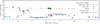 |
Fig. 1 Multi-mission X-ray+UV light curves during the SSS phase. UV data with UVM2 filter (2120 ± 500Å) were taken with Swift UVOT (ObsID ranges 00045788033–00045788053 and 00011558001–00011558021) and XMM-Newton OM (UV) and X-ray data over the energy range ~0.3−10 keV with AstroSat SXT (ObsIDs 9000003142 and 9000003160), Swift XRT, NICER (ObsIDs 2200810104 on day 18.3 and 2200810106 on day 21.3), and the MOS2 light curve extracted from our new XMM-Newton observation (see legend). The XMM-Newton MOS2 and OM UVM2 light curves were taken between two Swift observations but overlap with five AstroSat SXT observations. The high time resolution of the XMM-Newton observation demonstrates the high degree of variability in X-rays on timescales shorter than the Earth occultation gaps between Swift and AstroSat observations. Meanwhile, in the UV, a slow declining trend can be seen that is consistent in the Swift UVOT and XMM-Newton OM data (see Sect. 2 for discussion). |
3 Description of the data
The most robust information can be deduced from the data, without any bias from model assumptions. We thus present first the data in this section with qualitative results, while quantitative results can be found in Sect. 4.
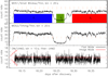 |
Fig. 2 XMM-Newton X-ray and UV light curves (units counts per second) extracted from MOS1 (small window, 200–850 eV range), MOS2 (timing mode, 200–850 eV range), and the optical monitor (image+fast mode with the UVM2 filter: ~ 1620−2620Å range). In the top panel, shaded areas mark three light curve segments analysed separately in Sect. 4.2. 22 short orange dotted vertical lines are spaced by 18.1 min (centred in the secondary dip within egress from the deep dip), corresponding to the frequency of 0.92 mHz discussed in Sect. 4.2. Of these 22 marks, eight (36%) correspond to an anomaly in the light curve (deep dip in- egress or small dip), while the duty cycle increases to 50% (5/10) after the dip, leading to a formally statistical detection. In the bottom panel, the high time resolution OM fast mode light curve is shown in black. Three OM Image mode exposures were taken simultaneously with each OM fast mode segment, and the average image mode count rates are shown with the horizontal orange lines covering the start+stop times. The red horizontal lines mark the magnitude range 12.97–12.99 within which the sources gradually fade from start to the end of the observation. This magnitude range is ~ 5 mag brighter than during quiescence (see text). See Sect. 3.1 for discussion. |
3.1 UV and X-ray light curves
The X-ray and UV light curves extracted from EPIC MOS and OM are shown in detail in Fig. 2. The initial steep rise and the deep dip are the most striking features in the X-ray light curves. The initial rise indicates the launch of the second SSS bright phase after a fainter interval of one day (Fig. 1, Singh et al. 2021). The deep dip lasted ~ 1 h, with steep ingress and egress and roughly constant emission in between. It was followed by a smaller dip within the rise back to the pre-dip count rate. Further smaller dips can be seen, at least one before and three after the main dip. The OM light curve shows a slow continuous declining trend from mag 12.97 and 12.99. The decline is consistent with the Swift UVOT data (see Fig. 1) yielding a decline rate of 0.1 mag per day. The UV light curve was unaffected by the events that caused the X-ray variability, which could mean that UV and X-ray emission come from different regions. If the X-ray dip was caused by an occulting body that moved in front of the regions emitting both UV and X-ray emission, it would consist of material that is optically thick only to X-rays. For example, as argued by Ness et al. (2012), neutral hydrogen is transparent to UV with energies < 13.5 eV while X-rays suffer photoelectric absorption depending on the column density.
3.2 High-resolution grating spectra
Common spectral analysis approaches of low-resolution CCD spectra are based on fitting a spectral model and drawing conclusions from the model. Meanwhile, high-resolution grating spectra allow us to draw conclusions directly from the data because individual emission and absorption lines can be resolved.
3.2.1 Overview and spectral evolution
In Fig. 3, we illustrate the time evolution of the RGS spectrum. We produced 48 RGS events files by filtering in adjacent time intervals of 500 s and extracted corresponding RGS spectra that are aligned as a time evolution map in the main panel visualising the spectral evolution. In the right panel, the light curve is shown along the vertical time axis with the count rate across and shadings marking time intervals from which a bright (light blue) and a dip spectrum (dark purple) have been extracted. The time stamp ranges are given for reproduction in mission time units (seconds since reference MJD 50 814 = 1998-01-01T00:00:00 TT) are (6.8490264−6.8490537) × 108 s for the dip spectrum (2.7 ks) and (6.8489253−6.8490220) × 108 s and (6.8490711−6.8491643) × 108 s for the bright spectra before and after the deep dip, respectively, with the summed exposure time of 19 ks. These ranges exclude the early rise and the dip. We also extracted RGS spectra during the three smaller dips after the deep dip, combining data from the time stamp ranges (6.8491072−6.849111) × 108 s, (6.8491183−6.8491218) × 108 s, and (6.8491287−6.8491318) × 108 s. Finally, we extracted a separate spectrum during the secondary dip within the egress part of the deep dip: time stamp range (6.8490613−6.8490688) × 108 s.
A blackbody model was fitted to the combined bright spectrum in an attempt to describe the overall spectral shape. To account for photoelectric absorption by the cold interstellar medium (ISM), we used the tbabs model by Wilms et al. (2000). The dominant ISM absorption is due to neutral hydrogen at energies above 13.6 eV (λ < 911Å), with exponentionally increasing transmission towards higher energies, thus affecting long wavelengths more than shorter wavelengths. The only model parameter is the neutral hydrogen column density NH, and we found a best fitting value of NH = 5.4 × 1021 cm−2. Photoelectric absorption by other elements are included in the tbabs model with default cosmic abundances. In order to best reproduce the O I absorption edge at 22.8 Å, we have reduced the abundance of oxygen by 30%. Since the tbabs model only accounts for neutral absorption, in order to reproduce the absorption edges of highly ionised N VI and N VII, two artificial absorption edges were included at 16.75 and 18.79 Å, with the column densities of 2.2 × 1017 cm−2 and 1.1 × 1017 cm−2, respectively, after manual adjustment. For the parameter Teff, we adopted a value of 6.9 × 10⁵ K, which roughly reproduces the overall spectral shape. We note that the assumed depths of edges and O I abundance have a strong effect on the best-fitting Teff and NH parameters as already noted by Page et al. (2020). We do not invest efforts into resolving the degeneracy of these model parameters as the (oversimplified) assumptions of a blackbody model are unphysical given the complex circumstances.
The blackbody fitting is not intended to derive physical quantities but to identify trends, similarly to Page et al. (2020), who studied the long evolutionary trends of, for example, Teff. In Fig. 4, we show the evolution of the observed spectrum-to-blackbody reference curve ratio. For each of the 48 sub-spectra, the same blackbody model was used as for the total spectrum, except for the normalisation, which was adapted to the brightness evolution. In the map, red and blue thus indicate excess above the blackbody line, while any light colours indicate reduced emission such as absorption lines. The vertical dashed lines guide the eye, demonstrating that absorption lines are blueshifted: N VII at 24.8 Å or O VII at 21.6 Å. Meanwhile, emission lines appearing strong relatively to the blackbody continuum during the dip are seen at rest wavelengths.
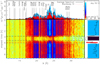 |
Fig. 3 Spectral time map based on 48 RGS spectra extracted from adjacent 500 s time intervals. The main panel shows the spectra with wavelength across, time down, and flux colour-coded following the non-linear colours shown as bars in the top rightpanel along the vertical flux axis. The shadings in the bottom right panel indicate time intervals from which the spectra shown in the same colour shadings in the top left panel have been extracted. In the top left panel, the total spectrum is also shown with a solid black line, and a simple blackbody fit is represented by the dotted red line. See Sect. 3.2.1 for details. |
3.2.2 Continued shock emission
The early shock emission before the SSS phase started was observed with Chandra on day 6.3 and was analysed by Orio et al. (2020). In Fig. 5, we show the hard part of the XMM-Newton RGS spectrum compared to the earlier Chandra HETGS spectrum. One can see that the Si and Mg XII lines have faded, while the (lower temperature) Mg XI and Ne lines are observed at about the same strengths; possibly also the (cooler) O VIII lines at 16 and 19 Å appear equally strong, although the Chandra HETGS has a very low sensitivity at those wavelengths. This is clearly a cooling effect as the Si XIV (log Tpeak = 7.2), Si XIII (log Tpeak = 7.0), and Mg XII (log Tpeak = 7.0) lines are formed at higher temperatures than the Mg XI (log Tpeak = 6.8), Ne X (log Tpeak = 6.8), and Ne IX (log Tpeak = 6.6) lines. The features at ~ 13.5Å may be either Ne IX or Fe XIX lines, the latter being formed at log Tpeak = 6.8 (Ness et al. 2003a). A slow reduction of temperature with time has been found from model fits to the X-ray spectra from the Swift monitoring campaign presented by Page et al. (2020). The asymmetric line profile of the Mg XII line appears to have become symmetric; however, close inspection of the line reveals that the profile is consistent with the RGS line spread function, and any asymmetry cannot be resolved with the RGS.
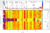 |
Fig. 4 Same as Fig. 3, where each of the 48 spectra were divided by a blackbody curve with the same parameters as the dotted red line in the top panel of Fig. 3, only re-normalised to the brightness of the respective spectrum. Wavelengths at which the ratio is below one indicate absorption lines; e.g., N VII at 24.8 Å, whereas wavelengthswith ratios greater than 1 indicate emission lines, that is, the same N VII or the N VI forbidden line at 29.1 Å duringthe dip. See Sect. 3.2.1 for details. |
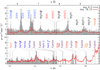 |
Fig. 5 Comparison of the pre-SSS Chandra HETG spectrum taken on day 6.3 (ObsID 22 845; Orio et al. 2020) and the XMM-Newton RGS spectrum taken on day 18.12. The line labels are placed at rest wavelengths using different colours for different elements for better distinction. See Sect. 3.2.2 for discussion. |
3.2.3 Identification of absorption and emission lines during the SSS phase
In Fig. 6, we compare the bright spectrum (blue line) and dip spectrum (dark green shadings) with RS Oph (light grey shadings) during the early SSS phase (Ness et al. 2007). Line labels of important transitions are marked in order to validate which of them are detected.
At short wavelengths λ < 16.5Å, the bright spectrum and the dip spectrum are identical, indicating that the shock spectrum shown in Fig. 5 was unaffected by the deep dip. This is a first indication that the cause of the dip is to be searched for near the surface of the white dwarf.
In the following, we describe absorption and emission lines from selected iso-electronic sequences. For the purpose of line identification, we ignore the blueshifts for the moment (thus line labels and observed features do not match exactly), while we measure them in Sect. 4.1.
The most prominent lines in SSS spectra of novae arise from the H-like Ly series of nitrogen, N VII: The Ly α (1s-2p) line at 24.78 Å can be seen both as a deep absorption line during the bright part and as an emission line in the dip spectrum. Also, the Ly β (1s-3p) line (20.90 Å) is likely detected as an absorption line, although there is a defect (chip gap) in the RGS1 at 20.81 Å3, and this wavelength range is not covered by the RGS2. The Ly γ (19.82 Å, 1s-4p) and Ly δ (19.36 Å, 1s-5p) lines are clearly seen in absorption, and the absorption edge at 18.6 Å is clearly visible.
Meanwhile, the He-like nitrogen lines, N VI, are much less dominant. While in RS Oph, the N VI 1s-2p line at 28.78 Å can clearly be seen in emission and absorption (also the intercombination and forbidden lines in emission), the features in the spectrum of V3890 Sgr cannot be clearly attributed to any of the N VI lines. It is possible that (see discussion later) diffuse line emission and absorption balance out. In fitting a blackbody continuum and looking at the residuals (see Fig. 4), an absorption feature at roughly the same blueshift as for N VII might be attributed to N VI He α4, and possibly also the intercombination and forbidden lines. The forbidden line of N VI He α at 29.54 Å especially appears prominent during the dip.
The N VIβ line at 24.9 Å blends with the N VIIα line and could contribute to the broad absorption feature. The emission line spectrum during the dip is dominated by the N VII line at 24.78 Å, while there is a somewhat weaker feature at 24.9 Å (best seen in Fig. 11) that appears to be N VI He β. Also, a weak N VI absorption line can be seen in the difference spectrum between bright and dip spectra (see right panel of Fig. 7). At the wavelengths of N VIγ (23.77 Å) and δ (23.28 Å), no convincing absorption feature is seen, as well as no edge at the ionisation energy of N VI to N VII at 22.46 Å.
The H-like Ly series lines of oxygen, O VIII, are clearly seen in RS Oph with the Ly α line at 18.97 Å, β at 16 Å, and possiblyγ at 16.77 Å. The SSS spectrum of V3890 Sgr has lower continuum at the wavelengths of the O VIII Ly series lines, but the Ly α and β lines can be seen in emission in the dip spectrum. Especially for the O VIII Ly β line, the emission in the dip and bright spectra are perfectly consistent with each other (as also the Fe XVII and Ne X lines). This indicates that the bright spectrum may be a composite of the dip emission and the photospheric SSS emission. Assuming the dip emission originates in the shock emission site (possibly a combination of collisional and photo-ionisation or excitation), the pure SSS spectrum can be reconstructed by subtracting the dip spectrum from the bright spectrum. The result is shown for the wavelength region around the O VIII Ly α line in the left panel of Fig. 7; the nearby O VII He β line at 18.62 Å is also included. While the bright spectrum shows little evidence of an absorption line, the difference spectrum clearly shows both lines as blueshifted saturated absorption lines. Also, the N VII and N VI blend (right panel) appears saturated with the two lines clearly separated as in the bright spectrum.
The He-like O VII He α line (21.6 Å) can clearly be seen in Fig. 6 in absorption and also in emission during the dip spectrum. The He β (18.62 Å) line is only seen as an absorption line in the difference spectrum (left panel of Fig. 7). The He γ and δ lines are clearly detected as blueshifted absorption lines with at best weak emission in the dip spectrum. They are suspiciously broad and deep, and one may wonder whether they could be contaminated by other lines; however, no transitions of sufficiently abundant elements with comparably high oscillator strengths are known at these wavelengths. There is no clear evidence of carbon lines from the various transitions marked in Fig. 6.
Other nova SSS spectra that have been studied in greater detail have shown absorption features that could not easily be identified see, e.g., Table 5 in Ness et al. (2011). We have searched for possible features around the wavelengths listed as projected wavelengths (thus assuming they are blueshifted by the same amount as known lines in the same spectra). In Fig. 8, we compare V3890 Sgr with two other novae and mark well-known and lesser known absorption features.
A feature at 26.93 Å listed in Table 5 of Ness et al. (2011) is seen in V3890 Sgr as possible blueshifted narrow absorption line and in V4743 Sgr as emission line at rest wavelength (see also Ness 2020). The Chianti atomic database (Dere et al. 2019) contains a C VI 1s-4p line (26.9 Å) and an Ar XV 2p-3d line at 27.04 Å. Since there are no other carbon lines detected, the Ar XV identification appears more likely. In emission, this line would be the strongest in the multiplet, while another Ar XV 2p-3d transition at 26.5 Å has a higher oscillator strength of gf = 5.1 and Chianti lists gf = 1.6 for the former transition. We do not see an absorption feature around 26.5 Å; either this is another unknown transition, or the oscillator strength in the Chianti database is incorrect.
The N VI 1s-2p line is only seen as a weak feature in V3890 Sgr (likely owing to overlapping weak SSS emission and strong emission from the shock regions, see discussion above) but as clear narrow blue-shifted absorption line in the other spectra, where some emission component can also be seen in SMC 2016 on day 38.9. The feature at 30.42 Å from Table 5 in Ness et al. (2011) can possibly be seen in V3890 Sgr but would not be identified as an absorption feature without the knowledge of an absorption line in other systems as can be seen in the spectra below. The Chianti database lists as possible candidates S XIV 2p-3d at 30.30 Å, S XIV 3s-3p at 30.43 Å, or Ca XI 2p-3d at 30.45 Å. The first transition has a high oscillator strength of gf = 4.6; however, the line would then be redshifted, against the trend of other lines. The second listed transition has a rather low oscillator strength of gf = 0.46, and stronger S XIV would need to be present. The Ca XI 2p-3d transition is the strongest in the multiplet and appears the most likely identification. The N I interstellar absorption line is always seen at 31.28 Å, but the continuum in V3890 Sgr is already quite weak.
A feature at ~32Å was not listed in Table 5 of Ness et al. (2011) but was discussed in Ness (2020) as being highly ‘mobile’; in SMC 2016, it disappeared between days 38.9 and 73.8, whereas in V4743 Sgr, it has shifted between days 180 and 197. This shift is shown in more detail in the top panel of Fig. 9 in velocity space. The location of the absorption line around 32 Å has changed by ~ 500 km s−1 within only two weeks. No other absorption line shifted by this amount (Ness 2020). The line is clearly detected in V3890 Sgr at lower blueshift, although the rest wavelength is obviously highly uncertain, and with only one observation we do not know whether such a shift may have occurred before or after this observation. The Chianti database lists as possible transitions S XIII 1s-3p at 32.24 Å or S XIV 2p-3d at 32.56 Å. The S XIII line with the highest oscillator strength is expected at 34.85 Å (gf = 5 compared to gf = 0.5 for the 32.24-Å line) where we do not see an absorption line, although the continuum is already very low. The S XIV 2p-3d line at 32.56 Å has a value of gf = 2.4, but another S XIV 2p-3d at 30.77 Å is listed with gf = 2.8, which is not as clearly seen.
In the bottom panel of Fig. 9, the 26.93 Å region is shown in comparison to RS Oph, where an absorption line only seen on day 40 had disappeared two weeks later. The rest wavelengths of the two lines are assumed here to yield the same blueshift in V3890 Sgr.
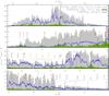 |
Fig. 6 Comparison of RGS spectra of V3890 Sgr extracted during the dip (dark green shadings) and during time intervals excluding the dip and the initial rise (blue line). The top panel shows the full spectral range of interest, while the panels below zoom in to show more detail. The light grey shading is the Chandra LETGS spectrum of RS Oph taken on day 39.7 after outburst (Chandra ObsID 7296), scaled down by a factor of 5. See Sect. 3.2.3 for discussion. Labels with different colours for different ions are included at their rest wavelengths. |
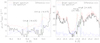 |
Fig. 7 Dip spectrum, shown with dotted blue lines, most likely represents emission that is also present during the bright spectrum (red dotted lines). It probably does not originate from the SSS photosphere but further outside, likely the shock emission site. As an illustration of how the pure SSS spectrum may look, the difference between bright and dip spectrum is shown with black solid lines for oxygen (left) and the nitrogen lines (right; see labels). See Sect. 3.2.3 for discussion. |
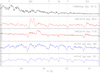 |
Fig. 8 Comparison of spectral range between 26 and 35 Å of V3890 Sgr with the novae SMC 2016 on days 38.9 (Chandra ObsID 19011) and 73.8 (XMM-Newton ObsID 0794180201) and V4743 Sgr on days 180 (Chandra ObsID 3775) and 197 (XMM-Newton ObsID 0127720501). Dotted vertical lines mark wavelengths of absorption features to draw attention to,with labels (only if unambiguously known) or question marks given at the top. See Sect. 3.2.3for discussion. |
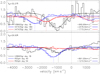 |
Fig. 9 Comparison of line profiles of unidentified lines. Top: assumed rest wavelength 32.27 Å compared to V4743 Sgr on days 180 (Chandra ObsID 3775) and 197 (XMM-Newton ObsID 0127720501). Bottom: assumed rest wavelength 26.93 Å compared to RS Oph on days 40 (Chandra ObsID 7296) and 54 (XMM-Newton ObsID 0410180301). See Sect. 3.2.3 for discussion. |
3.2.4 The dip spectrum
The dip spectrum is dominated by emission lines that can either be formed by collisional or radiative interactions. In Fig. 10, the dip spectrum is shown by zooming in on the He-like triplet lines of O VII, N VI, and Ne IX. The He-like triplets consist of a 1s 1S0-2p 1P1 resonance line, usually labelled with r, and two forbidden lines: an intercombination line 1s 1S0-2p 3P1 (thus forbidden spin flip), labelled as i and a forbidden line 1s 1S0-2s 3S1 (thus forbidden spin flip plus forbidden l = 0 transition), commonly labelled as f. The intercombination line was already seen in the 1960s in solar spectra as a result of the low density in which the correspondingly low collision rates allow enough time for the excited states of forbidden transitions to radiate back to the ground. Meanwhile, the forbidden line was not expected to be seen because of the even longer radiative de-excitation timescales, yet a strong line was seen at 22.1 Å leading Gabriel & Jordan (1969) to make careful calculations, ultimately demonstrating that the densities were indeed low enough to allow the forbidden line of O VII to be formed and to escape. The hugely different excitation and de-excitation probabilities of these lines, formed by the same element in the same ionisation stage, offer a wide range of plasma diagnostics independent of elemental abundance and of a plasma within a narrow temperature range. The various combinations of ratios are powerful plasma diagnostics, namely:
R = f∕i depends on the plasma density. At increasing density, the timescale for collisional excitations of 1s2s 3S1−1s2p 3P1 (thus f → i) becomes shorter than de-excitations 1s2s 3S1−1s2p 1P1 (f line to the ground), and the i line increases at the expense of the f line.
R = f∕i also depends on the intensity of the UV radiation field. The f → i can also be triggered by photons at the right energy which lies in the UV. Independent measurements of the UV intensity at the energy E(i) − E(f), combined with measurements of the R ratio allows calculation of the dilution factor and thus the distance between UV emission source and X-ray plasma.
G = (f + i)∕r depends on the plasma temperature in a collisional plasma. The collisional excitation probabilities of the r line depend differently on temperature than i and f lines.
G = (f + i)∕r is an indicator to distinguish photo-ionised from collisionally ionised plasmas. In a photoionised plasma, dominated by radiative recombination processes, the forbidden lines i and f are favoured over the r line, leading to a higher G ratio, whereas a collisional plasma yields G ~ 1.
In light of these rich diagnostics possibilities, we took a closer look at the He-like triplets of various ions that probe different temperature regions. The signal to noise is very low in the dip spectrum, owing to the short duration of the dip, and determination of accurate line fluxes is beyond reach. However, the detection or non-detection alone of one or the other line can give us qualitative information.
The best case is O VII, and this is therefore shown in the top panel of Fig. 10. The r and the f lines can clearly be seen, while the i line is not detected in the dip spectrum. Since all lines are broadened, any measured flux depends on the number of spectral bins included and would thus be highly uncertain. Nevertheless, the absence of the i and detection of r and f lines at about the same strength suggests we are dealing with a low-density plasma dominated by collisional interactions. Also, the intensity of any UV radiation at the site of O VII emission must be low.
The presence of a few bad pixels around 21.8 Å may cast some doubt on the non-detection of the i line, but we argue that the i line should also be broadened as the r and f lines, in which case we should see some emission outside the bad pixels. This can be seen in the bright spectrum (which also contains a suspicious pixel) where a broad emission feature can clearly be seen around the i line, which is in fact equally as strong as the f line. The r line can only be seen as an absorption line in the bright spectrum, while the emission line does not appear substantially stronger during the bright phaseas the i line. All thisevidence suggests that during the dip phase we only see the emission originating from the shocked plasma that is collisionally dominated, while during the bright phase we see additional photoexcited plasma.
The N VI and Ne IX lines probe cooler and hotter plasma, respectively, and are thus also of interest. For N VI, the only line that appears clearly detected is the i line and perhaps the f line, although both would be blue shifted by a few pixels (~ 500 km s−1). There is noemission feature that could be attributed to the r line which complicates the interpretation. The r line is possibly self-absorbed owing to a geometry preferably scattering out of the line of sight; this would not affect the i and f lines as they have lower radiative excitation probabilities. The bright spectrum shows a similarly confusing picture, and drawing any conclusions from the N VI triplet is thus difficult.
The Ne IX triplet can be blended with Fe XIX (see Ness et al. 2003a), but the apparent emission features appear in random places and may just be noise. Since the 13-Å region contains no SSS emission from the WD photosphere, the bright spectrum (of longer duration) should not be different and shows none of the apparent emission features. The effect of resonant scattering into the line of sight only during the dip spectrum appears unlikely in this case as none of the spikes can be associated with a resonance emission line. We thus consider the Ne IX triplet not detected.
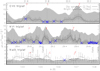 |
Fig. 10 He-like triplet lines of O VII (top), N VI (middle), and Ne IX (bottom) during the dip (black histogram, 2.7 ks) and during the bright time intervals (light shadings, 19 ks). The blue crosses mark bad pixels with suspicious or invalid flux values. Dotted vertical lines mark the resonance (r: 1s2p 1P1) intercombination (i: 1s2p 3P1), and forbidden (f: 1s2s 3S1) lines. In thebottom panel, potentially blending lines of Fe XIX are also marked and labelled. All spectra are smoothed with a Gaussian kernel of 0.03 Å, the instrumental broadening, for better visualisation. See Sect. 3.2.4 for discussion. |
4 Analysis
In the previous section, all conclusions that can be drawn directly from the data are presented. They are the most robust conclusions because they only depend on the quality of the data and calibration. In this section, we derive more quantitative conclusions that have a higher physical value but require models that depend on more assumptions and on the quality of atomic databases.
4.1 Absorption line profiles
The absorption line profiles provide information about the opacity distribution within the ejecta and thus the radial density distribution. It is important to assess the degree of complexity of the density profiles in the various absorption lines for the interpretation of global spectral models that usually assume some homogeneous density distribution in an easy-to-handle geometry (e.g. spherical symmetry).
We used the method described by Ness (2010) and Ness et al. (2011) to determine line shifts λshift, width λwidth, optical depths at line centre τc, and line column densities NX with results given in Table 2; columns show the ion name plus rest wavelength, line shift, line width, optical depth, oscillator strength, and ion column density. Additional rows marked with ‘add’ indicate that the model was added to the dip spectrum (see example in bottom right panel of Fig. 11), and ‘diff’ indicates that the absorption model was fitted to a difference spectrum (see example in bottom left panel of Fig. 11). The approach assumes a Gaussian optical depth profile τ(λ), and after fitting the parameters to the observations, NX is computed by integration over τ(λ) using oscillator strengths extracted from the Chianti database (Dere et al. 2019). The challenges when fitting the line profiles are how to deal with overlapping (blending) lines and how to account for the role of the dip spectrum that radiates emission which certainly should also be present during the bright spectrum.
In Fig. 11, four options are shown illustrating how to deal with the blended N VII Ly α (1s-2p) and N VI He β (1s-3p) lines. In the top left panel, a free fit of two line templates to the bright spectrum is shown yielding a good reproduction of the general shape of the broad absorption feature. The N VI absorption line comes out about half as broad as the N VII line. If the dip spectrum (dark green shaded) represents diffuse emission that is always present, the strong emission lines at the respective rest wavelengths of N VII and N VI could fill the red wing of the absorption feature, which would then mostly affect the blueshifted N VI line. In the bottom left panel of Fig. 11, the same two lines are fitted to the difference spectrum between bright and dip spectra (see right panel of Fig. 7), and the N VI line is now much broader, while the N VII line is narrower. A similar result is found when adding the model to the dip spectrum while fitting to the bright spectrum (bottom right panel). Note that the formal value of reduced χ2 is much smaller which is only partially owing to better fit. To properly account for the combined uncertainty of two data sets (bright and dip spectra), the error bars in each spectral bin are increased, and this may be an over-estimate. Finally, we also tested the possibility of a single line with the results shown in the top right panel yielding a visually good fit, although χ2 is slightly worse. The line blend is thus not well resolved.
As a comparison to RS Oph, in the top left panel we include two Chandra spectra taken at different times, indicated by grey shadings. One can clearly see that the overall absorption feature was much narrower in RS Oph. While the red wing essentially matches, the blue wing extends to much larger velocities in V3890 Sgr. On day 39 of the evolution of RS Oph (light grey), there was also an emission line component (Ness et al. 2007), but for RS Oph we were not lucky enough to separately see diffuse emission originating from outside the SSS atmosphere.
We performed the same fits to the bright spectrum while ignoring the dip spectrum and adding and subtracting it to or from the model to various absorption lines, and we summarise all results in Table 2. A graphical illustration of the results is shown in Fig. 12. It can be seen that most blueshifts cluster around 800−1500 km s−1 except for the N VIIα and possibly N VI He β line (with large uncertainty). It is also noteworthy that the 1s-2p transitions of N VII, O VII, and possibly N VI have a lower line column density than the transitions between higher principal quantum numbers and the ground, labelled as β, γ, and δ. Meanwhile, the line widths are mostly found within the 800−1500 km s−1 range, thus similar widths as shifts. The only outlier is O VII He-β, which is complicated to fit as the bright spectrum does not show any clear absorption feature. Whether or not there is an O VII He-β absorption line depends on the assumption that the diffuse emission line feature in the dip spectrum balances with a photospheric absorption line.
From the individual line profile analysis, we can conclude that there is a bulk velocity component of ~ 1000 km s−1 with a similar spread in velocities (line widths). The application of a global model assuming a single outflow component is thus justified (see Sect. 4.3).
4.2 Timing analysis
For the interpretation of the X-ray light curve (Fig. 2), we first applied an eclipse model assuming clumps crossing the line of sight as applied to the X-ray light curve of U Sco (Ness et al. 2012) in Sect. 4.2.1. We then checked for the presence of any periodic patterns in the light curve in Sect. 4.2.2.
4.2.1 Eclipse modelling
In this section, we assume obscuring bodies cause the large dip and the various smaller dips observed in the X-ray light curve (see Fig. 2). The spectrum during the central deep dip indeed suggests a total eclipse, as all soft photospheric emission has disappeared. Following the approach by Ness et al. (2012) for U Sco, for the modelling we assumed that the various dips in the light curve are caused by eclipses by spherical clumps orbiting around the white dwarf in circular orbits. Since obscuring bodies may be forming and disappearing, these assumptions may appear oversimplified, however the derived parameters of clump radius and orbital radius also correspond to the size of the clump and the distance from the white dwarf, even if not orbiting around the white dwarf. For the sake of simplicity, we assume an inclination angle of 90 degrees; moreover, we argue that the inclination angle is irrelevant for our purposes, as we only studied dips caused by clumps crossing the line of sight, while there may be many other clumps in the system.
If the central deep dip was caused by an orbiting body, it is tempting to interpret the initial rise in X-rays as an eclipse egress caused by the same body orbiting at a period of ~ 13.5 ks. However, if this period is stable, the next deep dip would then start its ingress still within the observation which is not observed. The initial rise to maximal SSS emission thus needs to be attributed to an additional body while the central dip could be associated with a large obscuring clump of orbital period P > 13.5 ks. We note, however, that the AstroSat light curve after the XMM-Newton observation contains no dips (see Fig. 1). The deep dip in the XMM-Newton observation fell exactly between two AstroSat data points, and we have not found any significant periodicity around 13.5 ks in the AstroSat light curve. It appears unlikely that all dips from an orbiting large clump would escape coverage by AstroSat. The occulting body having caused the large dip may have thus disappeared, or the next orbit may have been above or below the sight line.
A gravitationally bound system with a large body orbiting at P > 13.5 ks would be equivalent to  , with a the semi-major axis of the clump orbit, and MWD the white dwarf mass. We find the obscuring body in a wide orbit around the white dwarf primary, with a > 1.23 ⋅ R⊙ for a massive white dwarf MWD > M⊙, which is expected for a recurrent nova system with a recurrence timescale as short as V3890 Sgr. From the total eclipse duration one can estimate the size for this obscuring body to be r ≈ 2.8 ⋅ RWD, with RWD the white dwarf photospheric radius. This same result for the clump radius is recovered by fitting the ingress and egress light curve shapes, from which one can also find the tangential velocity for the obscuring body as vT = 1.3 × 10⁶ ⋅ (RWD∕R⊙) ms−1. For a circular orbit, this corresponds to an orbital radius of
  , which results in a = 161 ⋅ RWD when assuming a white dwarf mass MWD = 1.35 ⋅ M⊙ close to the Chandrasekhar mass limit and a photospheric radius RWD = 0.1 ⋅ R⊙ (see Page et al. 2020).
The observed X-ray (MOS2) light curve can be reproduced by a model including a compact white dwarf photosphere at a count rate of 26.20 counts per second, in addition to faint shock emission originating from a more extended region at 6.17 counts per second (see Sect. 3.2.4). The bright photospheric emission is dynamically obscured by multiple orbiting clumps, as the additional substructure in the central eclipse can only be modelled by introducing two smaller clumps next to the large orbiting body, with clump sizes as derived from the dip-depths. The eclipse modelling results are shown in Fig. 13, with the best-fit parameters provided in Table 3. The egress during the initial 420 s could be included in the model as an extra body (i.e. clump 0 in Table 3); however, these clump parameters are poorly constrained as the corresponding eclipse is not fully observed. Three additional clumps could be introduced to reproduce the three dips following the central eclipse. On the other hand, these dips could also be interpreted as oscillations linked to the white dwarf’s spin period (see Sect. 4.2.2). The best-fit model parameters provided in Table 3 face slight degeneracies in relation to the inclination of the orbital plane and the eccentricity of the orbit for each body, and so they do not form a unique solution. However, this model serves as a proof of concept for the straightforward interpretation of orbiting clumps causing the observed structure in the soft X-ray light curve.
The origin of the clumps could be similar to that of U Sco, i.e., we may be dealing with an accretion stream as part of a reforming accretion disc. The material within the stream may be clumpy. If the UV emission originates from the inner regions as in U Sco (evidenced by reduced UV emission during the primary eclipse), the absence of any corresponding clump occultations in the UV (Sect. 3.1) puts a strong constraint on the fabric of the clumps being of gasnature and transparent to UV while opaque to X-rays. Alternatively, the UV emission may originate from outside the inner regions or even be emitted by the clumps themselves and illuminated by the soft X-rays. Since in this model each clump is only seen once, the scenario of clump occultations is plausible but difficult to confirm.
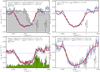 |
Fig. 11 Absorption line profile fitting to the bright spectrum (blue histogram) following the concepts described by Ness et al. (2011) for the two blended lines of N VII (λ0 = 24.78Å) and N VI (λ0 = 24.90Å); labels are included in the rest frame of the N VII line with black vertical lines. The respective best-fit models are shown with a thickred line, the assumed continuum level with the dashed blue line, and the model components for each line with dotted red lines. Top left: for comparison, Chandra spectra of RS Oph taken on days 39 (ObsID 7296, light grey) and 67 (ObsID 7297, dark grey) are included, re-scaled to the assumed continuum level showing the absorption line in V3890 Sgr was much broader. Top right: only a single line is fitted assuming that all contributions come from the N VII line. Bottom left: assuming the emission during the dip was also present during the bright phases, the dip spectrum is added to the model in each iteration step. The thin red dotted line represents the model spectrum without the addition of the dip spectrum. Bottom right: model fit to the difference spectrum in the right panel of Fig. 7. The fit results ofall lines are given in Table 2. See Sect. 4.1 for discussion. |
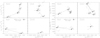 |
Fig. 12 Results from absorption line profile fitting showing the line column densities in the left panel and the line widths in the right panel, both as functions of line shift. The black data points represent the results when assuming the dip spectrum to represent a ‘background’ source of the level emission observed during the dip (see bottom left panel of Fig. 11). The 1σ error bars are large because the measurement uncertainties of both the bright and dip spectra are taken into account. The grey data points represent results from simple fitting to the bright spectrum (see top left panel of Fig. 11). The instrumental line broadening (of order 300 km s−1) has notbeen taken into account. Except for some outliers (see Sect. 4.1), a fairly uniform value of line blueshift and line width can be identified of the order of 800− 1500 km s−1, which is animportant finding in relation to the interpretation of the global spectral modelling results described in Sect. 4.3. |
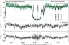 |
Fig. 13 Eclipse modelling for the XMM-Newton MOS2 X-ray light curve data of V3890 Sgr, with model parameters provided in Table 3; see Sect. 4.2.1 for discussion. |
4.2.2 Power spectrum analysis
In the top two panels of Fig. 2, 22 vertical tick marks are included that are separated by 18.1 min. Each of the smaller dips in all X-ray light curves, plus the ingress and egress parts of the dips, occur at one of these marks, suggesting a quasi-periodic behaviour. On the other hand, the majority of tick marks (14/22 = 64%) do not match any particular feature in the light curve. To substantiate this visual impression, in this section we describe a formal timing analysis performed using the Lomb-Scargle (L-S) method (Scargle 1982). The OM UVM2 light curve contains no periodic signal, and we thus focus on the X-ray timing analysis. The shaded areas in the top panel of Fig. 2 indicate three time segments that we analyse separately, the bright episode before the dip, the dip itself, and the bright episode after the dip. One can see thatthe variability behaviour changed after the dip, showing more smaller dips than before the deep dip.
Each time interval was de-trended with a third-order polynomial before computing the corresponding periodograms. For the time interval t2, during the dip, no periodic signal was found, and we thus focus on the pre- and post-dip time intervals, t1 and t3, respectively. In Fig. 14, we show the resulting periodograms, and in Table 4 we provide the derived frequency peaks above the 99% confidence level. Errors are estimated as the half width at half maximum of the power curve. Comparable values are aligned. Since the value of 0.92 mHz measured in the t3 interval of MOS2 agrees within the errors with both f3 and f4, it is placed in the middle. The pre-dip periodogram contains some peaks rising above the 90% confidence level; however, none of them are detected in both MOS1 and MOS2 light curves. We thus conclude that there is no significant periodic signal in the pre-dip light curve.
Meanwhile, the post-dip light curve contains three strong peaks in the power spectrum at frequencies below 2 mHz. The lowest frequency period of 47.6 min (f2 = 0.35 mHz) is detected consistently in both MOS1 and MOS2 light curves. This corresponds to a period of 2857 s, but the post-dip light curve only contains three cycles of variations, and we do not consider this sufficient evidence and thus discard this period from further studies. A period of 18.1 min (f3 = 0.92 mHz) appears as a single peak in the MOS2 light curve, while split into two signals at f3 = 0.85 mHz and f4 = 1.1 mHz and lower L-S power in the MOS1 light curve. The lower L-S power indicates a smaller amplitude, and that can be due to pile up. MOS1 operated in small window mode, which has a longer readout time than the timing mode that was used for MOS2. The longer readout time for MOS1 can lead to stronger pile up effects: two photons arriving within the readout time are registered as one photon with the sum of their energies. The distortion of the spectrum is the most critical effect, but it can also have an impact on the light curve as times of higher count rates suffer more pile up and a slight reduction in the count rate compared to times of lower count rates. This can reduce peaks in the light curve leading to a smaller amplitude in MOS1 compared to MOS2. We thus suspect the less significant peak in the MOS1 periodogram is a consequence of pile up and that both light curves are consistent with a frequency of 0.92 mHz, hence the 18.1-min cycle marked in Fig. 2. The frequency f5 is about twice 0.92 mHz, and we interpret this peak as the first harmonics of the 0.92 mHz frequency. Therefore, we conclude that the value of 0.92 mHz is the fundamental frequency, thus confirming the visual impression described above. While it is only detected in the light curve segment after the major dip, there is one smaller dip at approximately day 18.153, which coincides with one of the 18.1-min tick marks and may thus belong to the same cyclic behaviour.
In Fig. 15, we show phased and binned MOS1 and MOS2 light curves. The amplitude of the variations is of the order of 12%, with a slightly higher amplitude in the MOS2 light curve. As discussed above, this is likely due to pile up in the MOS1 detector, owing to the different mode.
As independent evidence for the 18.1-min period, we searched for this period in the AstroSat SXT data but did not detect it. This weakens the evidence, however, and we caution that a 10% amplitude of brightness variations is close to the limit of what can be detected with AstroSat.
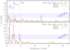 |
Fig. 14 Periodograms of the detrended light curve segments t1 (pre-dip, toppanel) and t3 (post-dip, bottom panel) computed from the respective MOS1 (black) and MOS2 (orange) data. Vertical blue dotted lines represent the detected frequencies f2 = 0.35 mHz and f3 = 0.92 mHz with its first harmonics 2 × f3 ~ 1.84 mHz (see Table 4). Horizontal blue lines represent the 90, 99, and 99.9% confidence levels. |
4.3 Spectral modelling
While the analysis in the previous section is closest to the data, we now attempt a global approach in which all atomic data are used in a self-consistent way based on the respective physical assumptions given in thefollowing sub-sections. The phenomenological spectral modelling was performed using the SPEX5 code (Kaastra et al. 1996, 2018) following the approach by Pinto et al. (2012) for V2491 Cyg.
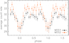 |
Fig. 15 Phased MOS1 and MOS2 light curves for the post-dip episode, t3, assuming the frequency of 0.92 mHz. The points represent averaged values with error of the mean. |
4.3.1 Spectral modelling of the dip spectrum
The observational evidence suggests the dip spectrum to be representative of a plasma located far enough outside of the atmosphericSSS emission to escape any occultations such that it is always present. To be consistent with a collisional plasma and that we have shown to have cooled (Fig. 5), the best candidate for this emission component are shocks whose emission was seen on day 6.3 with Chandra. Emission lines arising from ions formed at lower temperatures (such as O VII) can thus be expected to be stronger than in the Chandra observation on day 6.3 (Orio et al. 2020). These ‘cooler’ lines arise longwards of 18 Å, where the bright SSS emission is observed.
In Fig. 16, we show dip and bright spectra in log units to emphasise the fainter end of the emission. The red line is the best-fit APEC model to the earlier Chandra spectrum (Orio et al. 2020), folded through the RGS response without any re-scaling. It reproduces the range around the Ne X line of the (grey) dip spectrum on day 18.12 well but is brighter at shorter wavelengths and fainter at longer wavelengths. This indicates the cooling of the shocked ejecta. The yellow shaded area is the (down-scaled) bright spectrum, and it can clearly be seen that it deviates longwards of 17 Å. The blue curve is a best-fit model obtained with SPEX, which reproduces the faint and brighter parts of the dip spectrum well.
With SPEX, we have tested models including multiphase plasma in either collisional or photoionisation equilibrium.SPEX provides both a large database of atomic data and a powerful data fitting package based on the CSTAT parameter as a goodness of fit criterion. The CSTAT parameter scales well with χ2 and it does not depend on the assumption of Gaussian noise in the data. It assumes Poissonian statistics and is thus much more accurate if there are bins <25 counts. For a reference to the accuracy and power of CSTAT and its application to SPEX, see Kaastra (2017).
We describe the X-ray continuum with a blackbody component, BB. The absorption from the cold interstellar medium located along the line of sight towards V3890 Sgr and/or in its circumstellar medium is described with the HOT model in the SPEX nomenclature with a low temperature0.2 eV (e.g. Pinto et al. 2013) characterised by mainly neutral species.
Line emission (and/or absorption) from a plasma in photoionisation equilibrium is provided by the newly implemented and self-consistent PION6 model in SPEX, which is optimised to perform instantaneous calculation of ionisation balance, once a photoionising continuum is provided (inthis case the blackbody), and of the corresponding transmission and emission of the photoionised plasma. For the dip spectrum, which is dominated by emission lines, we chose the option to include only emission lines and not transmission in order to understand whether these can be described by gas in photoionisation balance. We found that a single PION component is not able to fit the strongest emission lines even if assuming exotic abundances and parameters.
We have also tested models of collisionally-ionised gas with a Gaussian or a power law-like emission measure distribution (GDEM and PDEM models in SPEX) but again without success. Non equilibrium models (NEI) also do not work, which means that separate model components are required. Particularly difficult is to simultaneously fit the resonance and forbidden lines of the O VII triplet and the Fe XVII L-shell lines at 15–17 Å. Moreover, the observed resonant lines seem fainter than their paired forbidden lines when compared to the model predictions. Since the models assume an optically thin plasma, the reduced resonance line emission relative to forbidden lines suggests resonant line scattering out of the sight line.
We achieved the qualitatively good fit illustrated with the blue line in Fig. 16 using an emission model consisting of two isothermal, collisionally ionised components (CIE models in SPEX nomenclature) and the parameters listed in Table 5. We also tested a model with photoionised components (PIE) that could be associated with the absorbing plasma in the (PION) component. However, CIE and PIE fits are statistically indistinguishable. In order to distinguish between CIE and PIE, we would need well-resolved He-like triplet lines; however, as discussed in Sect. 3.2.4 and seen in Fig. 10, the critical intercombination and forbidden lines are not well-enough resolved, owing to weak lines in contrast with the continuum and the resonance line self-absorbed by an unknown amount that is further complicated by the broadening of the lines. The weak conclusion in Sect. 3.2.4 is that during the dip, we only see the emission originating from the shocked plasma, hence our choice of the CIE components, while during the bright phase we might see additional photoexcited plasma.
The velocity dispersion of the two CIE components is tied in the fit and yields v = 890 ± 90 km s−1 with a line-of-sight velocity consistent with zero (i.e. at rest). The two added CIE contribute a total of ~ 1037 erg s−1 within 0.3–10 keV, assuming a distance of 9 kpc, while the blackbody has an X-ray luminosity of about 2 × 1037 erg s−1. The abundances are broadly consistent with Solar except for nitrogen, which is a factor of ~ 10 higher, as shown by its prominent emission lines, despite its cosmic abundance being lower than oxygen. The abundance scale used here is the default one in SPEX (protosolar, Lodders & Palme 2009). Enhanced N abundance is expected in CNO burning plasmas.
We caution that the error estimates in Table 5 are strictly statistical errors, not taking into account systematic effects. To obtain an idea of systematic effects, we performed several tests probing different scenarios. For example, with and without a PION component and variable or fixed values of NH and CF, we find areas between 8.2 × 1015 cm2 and 4.5 × 1018 cm2 and blackbody temperatures from kT = 62−125 eV. The parameters of the dip spectrum are thus not as well constrained as suggested from the formal errors. Statistically, the all-frozen configuration is not favoured, which is why we report the results with NH as a free parameter. However, there is only a difference of 30 in the CSTAT parameter between a model without a PION absorber and a PION with free NH. This means PION is statistically not required for the low-flux spectrum. Therefore, it is still possible (although not necessarily the truth) that something opaque stood in our line of sight obscuring the inner region (which was absorbed by PION) but not any other (cooler) scattered emission coming from outside and not absorbed by PION.
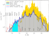 |
Fig. 16 Comparisons of spectral models with the dip (grey) and bright (yellow) spectra. The red line is the best-fit model to the earlier Chandra spectrum on day 6.3 (Orio et al. 2020), folded through the RGS response, and one can see that it has more hard emission and less soft emission than the dip spectrum on day 18.12. The blue line indicates the SPEX model for the dip spectrum, see Sect. 4.3.1 for discussion. |
RGS best-fit parameters to the two flux-resolved spectra.
4.3.2 Spectral modelling of the bright spectrum
The RGS spectrum of V3890 Sgr extracted during the high-flux intervals as indicated in Fig. 2 is characterised by strong blueshifted absorption lines carved into a super-soft X-ray continuum, with additional emission lines that appear primarily in the harder energy band below 17 Å. We also attempted to model the RGS spectrum extracted during this phase with SPEX following the approach of Pinto et al. (2012) for V2491 Cyg.
As described in Sect. 3.2.1, we adopted a blackbody continuum component (BB) and interstellar neutral absorption (HOT) with a low temperature parameter. Given the higher continuum in this spectral state and the strength of the oxygen K edge, we accounted for any dust or molecular gas absorption through the AMOL model in SPEX, which was necessary to correctly model the neutral O K edge in nova V2491 Cyg (Pinto et al. 2012) and in common X-ray binaries (Pinto et al. 2013). The line emission presumably produced by shocks around the nova and likely of collisional-ionisation nature is not included through a collisional-ionisation model but rather by using the low-flux dip spectrum as a template emission model that we include as an additive emission component, Fλ DIP. This choice was dictated by the fact that the emission lines do not seem to significantly change throughout the whole observation. The photospheric absorption lines produced in the nova ejecta were modelled with the PION model. Compared to the work previously done in nova V2491 Cyg (Pinto et al. 2012), this model represents an evolution of the XABS model used in that paper as PION calculates the ionisation balance instantaneously from the simultaneously fitted continuum. Previously, we needed to provide a given SED and pre-calculate the ionisation balance and the strength of the lines, thereby preventing us from obtaining constraints on both the shape of the ionising continuum and the properties of the ejecta.
The spectrum extracted outside the dips is therefore modelled with a multi-component model Fλ symbolicallydescribed as
 (1)
(1)
Free parameters are the column density, NH, and the oxygen abundance of the interstellar absorber (HOT). The strong O K edge around 23.0 Å and the 1s-2p line at 23.5 Å allow us to achieve high sensitivity on the contributions from oxygen, dust, and gas phases thanks to the relative ratio of the edge and line depths and the detailed shape of the edge. The column density of the dusty AMOL component is a free parameter. We tested several compounds (ice, iron oxides, silicates, and some carbon molecules) and achieved the best fit using silicates from pyroxene, although olivine provides comparable results. This agrees with previous results concerning nova V2491 Cyg and Galactic low-mass X-ray binaries (Pinto et al. 2012, 2013). The normalisation and the temperature of the blackbody were also free to vary. For the PION component, we fitted the column density, the ionisation parameter (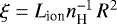 ), the outflow velocity, the velocity dispersion, and the abundances of the atomic species responsible for the detected lines (e.g. C, N, O, Si, S, Ar, Ca, Fe, Ni). We adopted solar abundances for all other species (X/H = 1) including neon and magnesium because the spectral continuum is too low below 15 Å to be sensitive to their absorption lines. This model is simpler than the one used for V2491 Cyg in Pinto et al. (2012), where we employed up to three layers of photoionised gas as there was a strong trend between the line blueshift and the corresponding ionisation potential. As can be seen from Fig. 12, the line blueshifts are rather homogeneous, except for the N VII line.
The best-fit model and residuals are shown in the top two panels of Fig. 17 with the best-fit parameters listed in the right column of Table 5. Our simple model provides a good description of the overall spectrum, matching the strengths and centroids of most absorption lines, yielding a reduced C statistic of C∕d.o.f. = 10 070∕1716 = 5.9, which is a substantial improvement on a model without PION absorption (C∕d.o.f. = 50548∕1693 = 30.0) or the simple blackbody model (C∕d.o.f. = 86 404.84∕1694 = 51.0). A reduced C-statistic value of 5.9 is not formally considered an acceptable fit, but we notice that given the high count rate of the source, any uncertainties in the RGS calibration, the atomic database (whose cross-sections are known to be uncertain up to the 20% level), or the structure of the outflow (i.e. in the case of a multi-phase plasma such as in V2491 Cyg), the presence of additional processes such as resonant scattering and photoionisation (re)emission will prevent us from achieving C∕d.o.f. ~ 1.
For the blackbody, we estimated a temperature of 90 ± 1 eV = 1 × 10⁶ K (similar to the SSS phase of V2491 Cyg, Pinto et al. 2012) and an X-ray luminosity of 178 × 1036 erg s−1, assuming isotropy and a distance of 9 kpc. For the cold interstellar medium, we estimate a column density NH = 4.3 ± 0.1 × 1021 cm−2, with the oxygen abundance slightly above the solar value and dust silicates contributing between 20 and 30% of the interstellar neutral oxygen as previously found in nova V2491 Cyg and most X-ray binaries (Pinto et al. 2012, 2013).
For the photoionised absorber, i.e. the nova ejecta, we estimated a column density NH = 18 ± 3 × 1021cm−2 and an ionisation parameter Log ξ = 2.29 ± 0.05 erg s−1 cm. For the outflow velocity and the velocity dispersion, we find − 900 ± 10 km s−1 and 350 ± 5 km s−1, respectively.Most element abundances are broadly consistent with the solar values, except for nitrogen (N/H ≳ 40) and oxygen (O/H ≳ 25). As previously shown for V2491 Cyg (Pinto et al. 2012), the absolute abundances (i.e. relative to hydrogen) may be subject to large uncertainties, particularly those driven by the knowledge of the exact continuum (flux and shape). However, the relative abundance ratios between atomic species responsible for the detected lines are much better constrained (e.g. O/N = 0.7 ± 0.1 and C/N = 0.11 ± 0.01, which is expected given the lack of strong carbon lines). The abundances obtained here have a pattern similar to the one measured for V2491 Cyg (Pinto et al. 2012).
We also fitted the same spectral model to the pre- and post-dip spectra separately (time intervals in Fig. 2 are marked in blue and red, respectively). We found all parameters consistent with each other, except for the velocity ΔV, for which we found − 870 ± 10 km s−1 before the dip and − 900 ± 10 km s−1 after the dip.
5 Summary of results
In summary, we obtain the following results directly from our observations:
The SSS emission is highly variable between two distinct brightness levels that we refer to as the bright phase and the dip phase. This short-term variability is consistent with Swift and AstroSat long-term light curves.
In the UVM2 band (~1620−2620Å), no such variability is seen on long-term or short-term timescales. A slow decline of 0.1 mag per day is seen.
The X-ray spectrum consists of bright SSS emission and emission lines from the cooling shocked plasma.
The emission lines from the shocks have evolved since a Chandra HETGS spectrum was taken on day 6.3. They show weaker emission in lines formed at higher temperatures and equal emission from lines formed at intermediate temperatures. The shocked plasma has thus cooled, consistently with expectations. Consequently, lines formed at lower temperatures should be stronger, but they arise at wavelengths where strong SSS emission is additionally seen. The SSS emission and the outer cooling shocks cannot easily be disentangled visually, except possibly during the dip. While the Chandra HETGS spectrum shows skewed emission line profiles, the XMM-Newton RGS resolution is not sufficient to resolve such a profile shape.
The SSS continuum shape resembles a blackbody with Teff~ 6.9 × 10⁵ K and NH~ 5.4 × 1021 cm−2 and ionisation edges from O I (interstellar, NH~ 4.3 × 1021 cm−2), N VI, and N VII (both local, 2.2 × 1017 cm−2 and 1.1 × 1017 cm−2, respectively).
Blueshifted broadened absorption lines can be identified from N VII Ly series and O VII He series. Weaker absorption features are likely also present fromO VIII Ly α and He-like N VI.
Absorption features seen at 26.93 Å, 30.42 Å, and 32 Å may arise from Ar XV, Ca XI, and S XIV, although these identifications are uncertain owing to discrepancies with other expected lines. These lines have also been seen in other SSS spectra, e.g., SMC 2016, V4743 Sgr, and RS Oph. The 32-Å lines especially seem highly ‘mobile’ with the ability to shift by as much as 500 km s−1 within two weeks.
The dip spectrum (2.7 ks duration) contains emission lines from Fe XVII, O VIII, O VII, N VII, and N VI.
At low significance, the He-like triplet lines of O VII suggest that the dip spectrum is dominated by collisional plasma at densities < 109 cm−3, while during the bright phases additional contributions from photoexcitations are seen.
The direct results from observations are more robust than model-dependent results, which in turn can give us more quantitative results.
Line profile fitting to individual absorption lines yields consistent line widths and blueshifts in most lines that correspond to a bulk velocity component of ~ 1000 km s−1. The line profiles are generally much more similar to each other than in V2491 Cyg, where at least three types of profiles were found (Ness et al. 2011). Nevertheless, some outliers are found, namely:
The absorption line complex at 24.8 Å, N VII Ly α, and N VI He β yields a particularly high value of line shift, while the line widths are consistent with all other lines.
Line column densities of 1s-2p transitions appear lower than transitions between ground-state and higher principal quantum numbers.
The column densities of absorption lines are about a factor of 2–5 lower than those of the absorption edges of N VI and N VII.
A power spectrum analysis of the light curve segment after the dip results in a significant detection of an 18.1 min period. Visual inspection of the whole light curve confirms several dips and the ingress and egress of the large dip and the initial rise to be in phase with this period. The duty cycle is low, with 36% in the whole light curve and 50% after the dip (including egress).
A global phenomenological spectral model implemented in SPEX was used to reproduce the observed dip and bright spectra.
During the bright episodes before and after the deep dip, the spectrum can be reproduced with a six-component model with 26 parameters. This is much less than the SPEX model fitted to V2492 Cyg (Pinto et al. 2012).
Assuming spherical symmetry and a distance of 9 kpc, the normalisation of the SPEX model implies a compact white dwarf of ~ 6000 km radius, which implies the photospheric radius to be close to the white dwarf surface.
The bolometric luminosity Lbol during the bright episodes, assuming a distance of 9 kpc, ranges mildly above the Eddington luminosity of a 1 M⊙ object.
The bright episode after the dip yields a slightly higher velocity derived from the blueshifts of the absorption lines compared to before the dip.
The dip spectrum contains emission lines that can be modelled with two collisional equilibrium components and a faint blackbody component. The observed X-ray flux of this component is a factor of ~ 10 fainter than during the bright phase, while the derived bolometric luminosity during the dip is a factor ~ 4 lower. Teff is much lower, while NH and emitting area are consistent within the uncertainties (see, however, the discussion on systematics in Sect. 6.2).
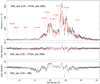 |
Fig. 17 XMM-Newton RGS spectrum of V3890 Sgr extracted during time intervals excluding the dip with the full SPEX model overlaid (top panel); for parameters, see Table 5. The rest-frame wavelengths of the dominant transitions are labelled. The middle panel shows the residuals, and the lower panel shows the residuals without the PION model. |
6 Discussion
6.1 Variability
Our results from Sect. 4.2.2 suggest small dips seen in Fig. 2 to be aligned with an 18.1 minute period, albeit at a low duty cycle and not supported by other data. An 18.1 minute period would be typical for the rotation period of the WD; however, the shape of the small dips cannot be explained by anything that would be co-rotating on the surface of the visible photosphere. Even small features would cause much broader phase profiles than those seen in Fig. 15. In this section, we discuss possible interpretations of the dips via clump occultation or surface features; however, none of them are necessarily periodic.
Ness et al. (2012) describe how deep dips in the U Sco X-ray light curve can be due to clumps passing through the line of sight that belong to an accretion stream within the ecliptic plane. This could be a periodic process which for U Sco could not be checked because less than one orbit had been observed. For V3890 Sgr, this scenario does not work because the orbit is much longer and the inclination angle is much lower than in U Sco. The clump model described in Sect. 4.2.1 thus assumes random clumps that are not necessarily in an orbit around the white dwarf, and in this model the small dips as well as the deep dip would coincidentally occur in a semi-regular cycle.
The spectrum in U Sco during the deep dips shows clear signs of scattered continuum emission, which in V3890 Sgr is much weaker during the dip. The intensity of the remaining continuum emission should be driven by the amount of surrounding scattering material of which there must then be much less than in U Sco.
Deep dips leading to the complete disappearance of SSS emission have also been seen in V4743 Sgr (Ness et al. 2003b) and V2491 Cyg (Ness et al. 2011). As these systems are also not edge-on systems like U Sco, it is plausible to conclude that a large number of occulting bodies would be distributed in all directions with no preference for the ecliptic plane. Only a very small fraction of them leads to observable dips, independently of the viewing direction.
What is more difficult is to understand why the minor dips all have similar profiles (see Fig. 15). In particular, having the same depth requires some fine-tuning of all clumps, which need to be of the same size and cross geometries to cause the same types of partial occultations. One may consider partial absorption as it is reasonable to assume that all clumps consist of the same material in similar physical conditions. However, partial occultation should be energy-dependent, and we would see a harder spectrum during the partial dips.
In the top panel of Fig. 18, the spectra during three of the minor dips is compared with the bright spectrum, and we do see energy-dependent absorption; however, this is not to the extent that would be expected for a partial absorber that would reduce the flux more at soft energies (longest wavelengths). Moreover we see the flux reduction at intermediate wavelengths, ~ 19−25.5Å. We tested some simple models, and this behaviour cannot be explained by simple absorption but requires some more complex processes. The simplest model we could find that can reproduce this behaviour is shown in the bottom panel of Fig. 18. It consists of the sum of a bright spectrum that is reduced by the same fraction (e.g. 10%) at all wavelengths and an additional cooler component. The sum of both components is then absorbed by the same column density of interstellar material.
This model experiment suggests that the small dips may not simply be absorption events but that a small fraction of the photospherecould temporarily be replaced by cooler plasma. Various possibilities could be imagined, examples include magnetic field lines suppressing convection as in the solar atmosphere (sun spots), material falling back through the photosphere creating temporarily cooler impact craters, or small compact plasma cells temporarily rising up from below the photosphere. If such plasma cells are more compressed than the rest of the photosphere, their photospheric temperature would be cooler. In all these examples, the sum of remaining photosphere and a smaller cooler component could produce dips with a spectrum similar to the red model in the bottom panel of Fig. 18.
These are only suggestions and would require deeper studies to test and validate them, which are beyond the scope ofthis work. Features such as sun spots appear unlikely to us as they would co-rotate with the white dwarf and form broader phase profiles than observed. That features such as sun spots could be so short-lived that each spot creates one dip appears rather unlikely to us. Material falling back appears possible, with each impact causing a dip; however, we cannot identify a situation in which this would be a semi-periodic process. Meanwhile, rising plasma cells might be controlled in some way by the rotation of the WD if some latitudes are more favourable to such rising cells than others. However, they would have to dissolve on timescales of the dip duration (~ 5 min). We can therefore think of various processes causing major and minor dips but do not have enough observational evidence to explain why these processes would occur periodically.
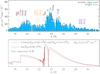 |
Fig. 18 Illustration of spectral changes with the small dips. Top: comparison of spectra extracted during the bright intervals (black histogram) and during three smaller dips after the deep dip (light blue). The emission only deviates at intermediate wavelengths but is similar at long wavelengths (driven by NH) and at short wavelengths (driven by Teff and edge absorption). Bottom: Ad hoc model to attempt to reproduce this behaviour. The black curve represents a blackbody curve (in arbitrary flux units) with the best-fit parameters to the observed bright spectrum. The red curve represents the sum of the black curve, reduced by 10%, and a blackbody spectrum with a lower temperature but absorbed by the same NH (see legend for values). The red model could be compared to the spectrum extracted during the smaller dips. See Sect. 6.1 for discussion. |
6.2 Spectroscopy
Super-soft-source spectra, at the time of their discovery, appeared to be quite easy to parameterise with blackbody fits that yielded good reproduction of observed CCD-type spectra (e.g. Krautter et al. 1996). The strongest reason for developing more complex models to fit CCD spectra of SSS spectra were the unrealistically high bolometric luminosities (Lbol) derived from the effective temperature (Teff) of blackbody fits. The fit quality from fitting LTE and NLTE models has not always improved, but more realistic bolometric luminosities (Lbol) were derived (e.g. Balman et al. 1998; Parmar et al. 1997, 1998). Since the fit quality has not improved, the lower values of Lbol were not required by the data but were a result of expectations. The only conclusion that can be drawn is that super-Eddington luminosities are not required by the data, but they are only ruled out by theory. Therefore, the higher spectral resolution of the Chandra and XMM-Newton gratings promised a breakthrough; however, the grating spectra turned out to be notoriously complex, and so far no model has been found that yields a statistically significant fit. A simple blackbody fit still reproduces the general shape fairly well, although no longer at a  level. However, no self-consistent atmosphere model that should reproduce the resolved absorption lines has come anywhere near
  .
.
Visual inspection is therefore not just pedantry but is needed to conceptualise the modelling approach. We should not be driven only by theoretical expectations, we also need to take into account strategic details such as weak forbidden lines or small line shifts that do not contribute significantly to χ2 of a global fit. A key result from the inspection of individual absorption lines is the finding that most lines are shifted by the same amount of ~ 800−1500 km s−1. In contrast, for V2491 Cyg, Ness et al. (2011) found a wide range of line shifts (see their Fig. 10), and a global model presented by Pinto et al. (2012) required a high number of layers.
The SPEX model presented by Pinto et al. (2012) may be a good compromise between an oversimplified blackbody fit and a complex atmosphere model. Just like an atmosphere model, it starts with a blackbody source function but then only adds phenomenological absorbing layers rather than computing the results of full-fledged radiative transport processes. While this approach is not fully physically self-consistent, the full (known) atomic physics is accounted for when fitting the absorption lines and edges. The reproduction of the data was much better than any atmosphere model to date; however, the number of layers was rather high, giving the impression of arbitrarily adding components until the data are reproduced. Thanks to the prior inspection of the individual absorption lines, this can be understood as dealing with multiple velocity components.
In this work, we were able to find a model with a single absorbing layer which is consistent with the findings from individual lines. The CSTAT value of ~6 is, strictly speaking, still not an acceptable fit, but it is much better than anything seen before when fitting models to SSS grating spectra. We also attempted to fit atmosphere models but failed to find anything close to an acceptable fit to the data. Nevertheless, Teff is in rough agreement with the SPEX result.
From both direct inspection and global model approaches, we can thus conclude that, compared to V2491 Cyg (Pinto et al. 2012), the atmosphere of V3890 Sgr appears relatively uniform. The good fit quality allows quantitative conclusions from the resulting parameters listed in Table 5; however, this is always with the caveat that the conclusions are model dependent (see below).
We are dealing with a hot atmosphere, close to a million degrees, much higher than Teff of a blackbody fit, which confirms many findings of blackbody fits underestimating Teff. This is quite easy to understand: a model ignoring the effects of the absorbing layers above the central source function that remove emission at the high-energy end of the Wien tail (e.g. by ionisation edges) needs to place the Wien tail of the source function at lower energies, and thus lower Teff. Models accounting for absorption edges will thus always lead to high Teff. Through temperature scaling with the fourth power while the radius is only squared, Lbol will be underestimated. The inclusion of ionisation edges in a blackbody fit is only the first step towards physically realistic model conditions. Apparently, accounting for all (known) absorbing atomic and ionic transitions in an arbitrary absorption layer can lead to a more adequate estimation of Teff of the underlying source function leading to similar results as a fully fledged radiation transport model. Very possibly, the exact radiation transport processes may not be the decisive factor when finding realistic Teff and thus Lbol.
The resulting photospheric radius falls into the ball park of typical white dwarf radii suggesting that the observed continuum emission originates from close to the surface of the white dwarf. This result assumes the emission to homogeneously be emitted by a spherically symmetric photosphere. If the symmetry assumption is not valid, then all estimates of radius and luminosities are invalid, and we may be dealing with much smaller emitting regions, each of them with luminosities much lower than 1038 erg s−1.
The dip spectrum, dominated by emission lines, can only be reproduced if the presence of an additional atmosphere is assumed and modelled in SPEX with a blackbody source function and the same PION absorption layer with the same parameters obtained from the bright spectrum. The X-ray flux of this component has decreased by a factor of ~ 10, while Lbol has only decreased by a factor of 4. Since the radius remained the same, the reduction in Lbol is thus owed only to the reduction of Teff 7. The reduction of LX by a factor of 10 is due to the fact that the peak of the spectral energy distribution has shifted into the FUV, where a larger fraction of flux is lost to the interstellar medium by means of photoelectric absorption by neutral hydrogen. A quick check comparing blackbody spectra with Teff = 10.4 × 10⁵ K and 7.2 × 10⁵ K (yielding a factor 4 in Lbol) yields a factor of 22 in LX assuming NH = 4.25 × 1021 cm−2. Therefore, at least within the statistical uncertainties, the deep dip could be explained by a reduced temperature alone without any other factor such as occultations that are assumed in Sect. 4.2.1.
The interpretation of the dip by reduced Teff alone and a corresponding reduction in Lbol implies a reduction in the nuclear burning rate as this is the only available energy source. A reduction by a factor of 4 on such short time scales defies physical principles of thermodynamic cooling and appears impossible to reproduce with nova evolution models.
Meanwhile, in the occultation model for U Sco, the observed blackbody-shaped continuum emission was interpreted by Thomson scattering in the ambient medium. This, however, would lead to a smaller radius (that is derived from the normalisation), while Teff would be unchanged. If, however, we are not dealing with Thomson scattering but significant contributions from Compton scattering, the photon energies would be reduced with each scattering event, leading to a softer spectrum that would yield lower Teff. This would lead to an apparent reduction in flux, and a reduced radius would not be needed. For photons well below 511 keV, as in our case, a single Compton scattering event does reduce the photon energy sufficiently to lead to such a large reduction in measured effective temperature; thus, multiple scattering events would be needed, as found in an optically thick photoionised blob. Since treating the radiative transfer with Compton redistribution is complex, we are unable to assess the viability of Compton scattering in detail, but we refer the reader to Suleimanov et al. (2006) for more work on Compton versus Thomson scattering in white dwarfs.
It is thus not necessary to give up the concept of constant bolometric luminosity, and it would need to be revisited if the assumption of Thomson scattering for the spectral analysis of U Sco could actually be replaced by Compton scattering. For U Sco, however, we do not have the original photospheric spectrum and a comparison is not so straight forward as in the case of V3890 Sgr.
As cautioned before, these conclusions are model dependent, and the uncertainty ranges given in Table 5 are only statistical uncertainties; thus, with 68% likelihood, results within these ranges are found again when repeating the fit with the same data and the same model. The accuracy of the values also depends on the quality and completeness of underlying atomic data and calibration uncertainty in the observations that are more difficult to quantify. Furthermore, the model assumptions may be different from reality, in which case none of the conclusions hold. Incorrect model assumptions can of course not be quantified. As an example, the intrinsic value of NH was found much lower in the dip spectrum (< 0.6 × 1021 cm−2) than in the bright spectrum (18 ± 3 × 1021 cm−2; see Table 5). Lower NH allows more soft emission to pass the interstellar medium, which can then lead to a lower temperature. Fixing NH to the value of the bright spectrum yields the same or even higher value of Teff for the dip spectrum, which does then not require the conclusion of Compton rather than Thomson scattering. The result thus depends strongly on the details of modelling photoelectric absorption.
7 Summary and conclusions
The third recorded outburst of V3890 Sgr has been observed in X-rays with Swift, AstroSat, NICER, Chandra, and XMM-Newton. All these observatories consistently found a slowly fading hard collisional emission line spectrum and a highly variable super-soft source atmospheric emission spectrum. All evidence supports that the collisional emission originates from shocks between the nova ejecta and the dense wind of the giant stellar companion star. The SSS spectrum is consistent with emission powered by residual nuclear burning on the surface of the white dwarf. Meanwhile, Swift UVOT and XMM-Newton OM light curves show a slow, smooth decline in UV as in the collisional X-ray emission. The UV emission is thus unrelated to the SSS emission from the white dwarf, both in terms of direct emission and inelastic scattering. The high-resolution XMM-Newton RGS spectrum revealed a clear reduction of the shock temperature compared to an earlier Chandra HETGS observation.
The focus of this work is on the timing and spectral analysis of the XMM-Newton data of the SSS component. The high degree of variability of the SSS component manifests itself in the XMM-Newton X-ray light curves as variations up to a factor of 4 between a bright state (65% of the time) and two low states (12% of the time), dominated by one deep dip in the middle of the observation and a likely similar dip that is only seen in egress at the start of the observation.
A possible 18.1-min oscillation During the bright phases, we see variations of the order of 10% that appear periodic with 18.1-minutes and are formally statistically significant after the deep dip but with a low duty cycle. This period was not found in the long-term AstroSat SXT data; however, a 10% brightness variation is close to the limit of what can be detected with AstroSat. Possible interpretations may be pulsations from the surface of the white dwarf (possibly related to the rotation of the white dwarf) that are damped while propagating to the outer layers. If the photospheric radius has shrunk after recovering from the deep dip, the amplitude of the dampened pulsations, then at lower radius, might have increased and become detectable.
Another interpretation may be the presence of slightly denser (and thus cooler) co-rotating bulges (e.g. at the magnetic poles) that are buried within the optically thick envelope until the photospheric radius shrinks to a critical limit. Again, if the recovery from the deep dip has resulted in a smaller photospheric radius, one or both co-rotating bulges would have become visible and would thus modulate the light curve with the white dwarf rotation period.
Eclipses by clumps are another possibility to explain the high-amplitude variations. Clump formation is expected in photoionised winds as in O stars, and a phenomenological eclipse model with seven clumps rotating on orbits between 5 and 150 times the radius of the white dwarf and sizes between 0.5 and 10 times the radius of the white dwarf can reproduce the observed light curve. In the model, each clump only crosses the line of sight once as the respective orbital periods are longer than the observation duration. Since the spectral shape with given energy of the Wien tail dictates that the central source must be very small, partial eclipses require a certain amount of fine-tuning; however, the system likely contains a much higher number than seven clumps, and only a small fraction of them will lead to partial or total eclipses.
The dip spectrum is dominated by mildly broadened emission lines at rest wavelengths, indicating that all SSS photospheric emission has disappeared, leaving behind ‘coronal’ emission originating from the cooler components of the shock plasma and possibly photoionised thin ejecta. The phenomenon of total disappearance of SSS emission during short periods of time has been observed before, in V4743 Sgr or RS Oph, for example. The steep recovery of emission to pre-dip levels after such dips supports interpretations of geometrical occultations compared to such abrupt changes in the nuclear burning rate. In the high-inclination U Sco system, the X-ray spectrum was constantly dominated by such emission lines and was interpreted as obscuration of the central SSS emission by the accretion disc or stream. Residual blackbody emission was seen and interpreted as Thomson scattering, and a weak blackbody component can also be identified in V3890 Sgr, although only with a spectral model (see below).
The photospheric X-ray absorption lines are resolved in the XMM-Newton RGS spectrum and are systematically blueshifted by ~ 800−1500 km s−1 and broadened within the same range. Other novae such as V2491 Cyg are much less homogeneous in these parameters, and this simplifies the spectral modeling.
The measurement of these velocity values is compromised by the relatively strong ‘coronal’ background emission lines seen at rest wavelengths during the dip, which then fill up the red wings of the blueshifted absorption lines, making them appear narrower than they would be when leaving the photosphere.
The SPEX modelling results in highly satisfactory reproduction of the complex SSS RGS spectrum with a relatively low number of components assuming a blackbody source function that is absorbed by a single photoionised layer (called PION in SPEX); for comparison, for V2491 Cyg, three PION layers had to be assumed. The CNO abundances were found to be non-solar, as is expected for nuclearly processed material. The shock component is also overabundant in N but less than in the photosphereindicating mixing between CNO-enrichted nova ejecta and solar-composition material from the companion star.
The SPEX model was also used to probe spectral changes with the variability patterns. In the deep-dip spectrum, a blackbody component can be detected, yielding a similar surface area but lower Teff compared to the bright spectrum. This implies a reduced value of Lbol and thus a reduced nuclear burning rate, which may be difficult to achieve on the short timescales of ingress and egress of the deep dip. The SPEX results and the clump occultation model combined lead to the picture of total occultation of the central source and Compton scattering ofphotospheric emission in the ambient, electron-rich medium. Compton scattering leads to a softer spectrum and thus lower Teff and reduced brightness, without the need for reduced Lbol.
The SPEX model also detected a small increase in blueshift of absorption lines from 870 ± 10 km s−1 before the dip to 900 ± 10 km s−1 after the dip. This supports interpretations of a smaller photospheric radius after recuperation from the dip which would also support both hypotheses for seeing 18.1 min oscillations only after the dip. Possible speculation might be that a large occulting clump has ripped off a small amount of plasma from the photospheric layers as a result of a grazing passage, or that it was ejected from the optically thick envelope.
Finally, the mystery of fast and high-amplitude variations started with the steep decline in a 2002 Chandra observation of V4743 Sgr and culminated with high-amplitude variability in the 2006 Swift monitoring observations of RS Oph. We show that the concept of constant Lbol does not need to be given up on, as such steep brightness variations can be caused by occultations, while the reduced photospheric temperaturein the scattered light can be explained by Compton scattering processes.
Acknowledgements
A.P.B., J.P.O., K.L.P. acknowledge support from the UK Space Agency. M.H. acknowledges support from an ESA fellowship. A.D. and P.B. were supported by the Slovak grant VEGA 1/0408/20, and by the Operational Programme Research and Innovation for the project: Scientific and Research Centre of Excellence SlovakION for Material and Interdisciplinary Research”, code of the project ITMS2014+: 313011W085 co-financed by the European Regional Development Fund. S.S. gratefully acknowledges partial support from NSF and NASA grants to ASU. BV gratefully acknowledges support by the Research Foundation – Flanders (FWO-Vlaanderen, project 11H2121N).
References
- Balman, S., Krautter, J., & Ögelman, H. 1998, ApJ, 499, 395 [NASA ADS] [CrossRef] [Google Scholar]
- Dere, K. P., Del Zanna, G., Young, P. R., Landi, E., & Sutherland, R. S. 2019, ApJS, 241, 22 [Google Scholar]
- Dobrotka, A., & Ness, J.-U. 2017, MNRAS, 467, 4865 [Google Scholar]
- Gabriel, A. H., & Jordan, C. 1969, MNRAS, 145, 241 [Google Scholar]
- Kaastra, J. S. 2017, A&A, 605, A51 [NASA ADS] [CrossRef] [EDP Sciences] [Google Scholar]
- Kaastra, J. S., Mewe, R., & Nieuwenhuijzen, H. 1996, in UV and X-ray Spectroscopy of Astrophysical and Laboratory Plasmas, eds. K. Yamashita, & T. Watanabe (Cambridge: Cambridge University Press), 411 [Google Scholar]
- Kaastra, J. S., Raassen, A. J. J., de Plaa, J., & Gu, L. 2018, SPEX X-ray spectral fitting package [Google Scholar]
- Krautter, J., Ögelman, H., Starrfield, S., Wichmann, R., & Pfeffermann, E. 1996, ApJ, 456, 788 [NASA ADS] [CrossRef] [Google Scholar]
- Lodders, K., & Palme, H. 2009, Meteorit. Planet. Sci. Suppl., 72, 5154 [Google Scholar]
- Mikołajewska, J., Iłkiewicz, K., Gałan, C., et al. 2021, MNRAS, 504, 2122 [CrossRef] [Google Scholar]
- Ness, J. 2010, Astron. Nachr., 331, 179 [NASA ADS] [CrossRef] [Google Scholar]
- Ness, J.-U. 2020, Adv. Space Res., 66, 1202 [NASA ADS] [CrossRef] [Google Scholar]
- Ness, J., Brickhouse, N. S., Drake, J. J., & Huenemoerder, D. P. 2003a, ApJ, 598, 1277 [NASA ADS] [CrossRef] [Google Scholar]
- Ness, J., Starrfield, S., Burwitz, V., et al. 2003b, ApJ, 594, L127 [Google Scholar]
- Ness, J., Starrfield, S., Beardmore, A., et al. 2007, ApJ, 665, 1334 [NASA ADS] [CrossRef] [Google Scholar]
- Ness, J.-U., Osborne, J. P., Dobrotka, A., et al. 2011, ApJ, 733, 70 [NASA ADS] [CrossRef] [Google Scholar]
- Ness, J., Schaefer, B. E., Dobrotka, A., et al. 2012, ApJ, 745, 43 [NASA ADS] [CrossRef] [Google Scholar]
- Orio, M., Drake, J. J., Ness, J. U., et al. 2020, ApJ, 895, 80 [NASA ADS] [CrossRef] [Google Scholar]
- Osborne, J. P., Page, K. L., Beardmore, A. P., et al. 2011, ApJ, 727, 124 [NASA ADS] [CrossRef] [Google Scholar]
- Page, K. L., Beardmore, A. P., Osborne, J. P., et al. 2019, ATel, 13084, 1 [NASA ADS] [Google Scholar]
- Page, K. L., Kuin, N. P. M., Beardmore, A. P., et al. 2020, MNRAS, 499, 4814 [CrossRef] [Google Scholar]
- Parmar, A. N., Kahabka, P., Hartmann, H. W., et al. 1997, A&A, 323, L33 [NASA ADS] [Google Scholar]
- Parmar, A. N., Kahabka, P., Hartmann, H. W., Heise, J., & Taylor, B. G. 1998, A&A, 332, 199 [NASA ADS] [Google Scholar]
- Pinto, C., Ness, J.-U., Verbunt, F., et al. 2012, A&A, 543, A134 [NASA ADS] [CrossRef] [EDP Sciences] [Google Scholar]
- Pinto, C., Kaastra, J. S., Costantini, E., & de Vries, C., 2013, A&A, 551, A25 [NASA ADS] [CrossRef] [EDP Sciences] [Google Scholar]
- Scargle, J. D. 1982, ApJ, 263, 835 [Google Scholar]
- Schaefer, B. E. 2009, ApJ, 697, 721 [NASA ADS] [CrossRef] [Google Scholar]
- Schaefer, B. E. 2018, MNRAS, 481, 3033 [NASA ADS] [CrossRef] [Google Scholar]
- Singh, K. P., Girish, V., Pavana, M., et al. 2021, MNRAS, 501, 36 [Google Scholar]
- Starrfield, S., Iliadis, C., & Hix, W. R. 2008, in Classical Novae, ed. M. Bode, & A. Evans (Cambridge: Cambridge University Press), 77 [CrossRef] [Google Scholar]
- Strader, J., Chomiuk, L., Aydi, E., et al. 2019, ATel, 13 047, 1 [Google Scholar]
- Suleimanov, V., Madej, J., Drake, J. J., Rauch, T., & Werner, K. 2006, A&A, 455, 679 [NASA ADS] [CrossRef] [EDP Sciences] [Google Scholar]
- Wilms, J., Allen, A., & McCray, R. 2000, ApJ, 542, 914 [Google Scholar]
XMM-Newton is an ESA science mission with instruments and contributions directly funded by ESA Member States and NASA.
He α denotes a 1s-2p transition in a He-like ion, He β 1s-3p, etc.
With values from Table 5, 
All Tables
All Figures
|
Fig. 1 Multi-mission X-ray+UV light curves during the SSS phase. UV data with UVM2 filter (2120 ± 500Å) were taken with Swift UVOT (ObsID ranges 00045788033–00045788053 and 00011558001–00011558021) and XMM-Newton OM (UV) and X-ray data over the energy range ~0.3−10 keV with AstroSat SXT (ObsIDs 9000003142 and 9000003160), Swift XRT, NICER (ObsIDs 2200810104 on day 18.3 and 2200810106 on day 21.3), and the MOS2 light curve extracted from our new XMM-Newton observation (see legend). The XMM-Newton MOS2 and OM UVM2 light curves were taken between two Swift observations but overlap with five AstroSat SXT observations. The high time resolution of the XMM-Newton observation demonstrates the high degree of variability in X-rays on timescales shorter than the Earth occultation gaps between Swift and AstroSat observations. Meanwhile, in the UV, a slow declining trend can be seen that is consistent in the Swift UVOT and XMM-Newton OM data (see Sect. 2 for discussion). |
| In the text | |
|
Fig. 2 XMM-Newton X-ray and UV light curves (units counts per second) extracted from MOS1 (small window, 200–850 eV range), MOS2 (timing mode, 200–850 eV range), and the optical monitor (image+fast mode with the UVM2 filter: ~ 1620−2620Å range). In the top panel, shaded areas mark three light curve segments analysed separately in Sect. 4.2. 22 short orange dotted vertical lines are spaced by 18.1 min (centred in the secondary dip within egress from the deep dip), corresponding to the frequency of 0.92 mHz discussed in Sect. 4.2. Of these 22 marks, eight (36%) correspond to an anomaly in the light curve (deep dip in- egress or small dip), while the duty cycle increases to 50% (5/10) after the dip, leading to a formally statistical detection. In the bottom panel, the high time resolution OM fast mode light curve is shown in black. Three OM Image mode exposures were taken simultaneously with each OM fast mode segment, and the average image mode count rates are shown with the horizontal orange lines covering the start+stop times. The red horizontal lines mark the magnitude range 12.97–12.99 within which the sources gradually fade from start to the end of the observation. This magnitude range is ~ 5 mag brighter than during quiescence (see text). See Sect. 3.1 for discussion. |
| In the text | |
|
Fig. 3 Spectral time map based on 48 RGS spectra extracted from adjacent 500 s time intervals. The main panel shows the spectra with wavelength across, time down, and flux colour-coded following the non-linear colours shown as bars in the top rightpanel along the vertical flux axis. The shadings in the bottom right panel indicate time intervals from which the spectra shown in the same colour shadings in the top left panel have been extracted. In the top left panel, the total spectrum is also shown with a solid black line, and a simple blackbody fit is represented by the dotted red line. See Sect. 3.2.1 for details. |
| In the text | |
|
Fig. 4 Same as Fig. 3, where each of the 48 spectra were divided by a blackbody curve with the same parameters as the dotted red line in the top panel of Fig. 3, only re-normalised to the brightness of the respective spectrum. Wavelengths at which the ratio is below one indicate absorption lines; e.g., N VII at 24.8 Å, whereas wavelengthswith ratios greater than 1 indicate emission lines, that is, the same N VII or the N VI forbidden line at 29.1 Å duringthe dip. See Sect. 3.2.1 for details. |
| In the text | |
|
Fig. 5 Comparison of the pre-SSS Chandra HETG spectrum taken on day 6.3 (ObsID 22 845; Orio et al. 2020) and the XMM-Newton RGS spectrum taken on day 18.12. The line labels are placed at rest wavelengths using different colours for different elements for better distinction. See Sect. 3.2.2 for discussion. |
| In the text | |
|
Fig. 6 Comparison of RGS spectra of V3890 Sgr extracted during the dip (dark green shadings) and during time intervals excluding the dip and the initial rise (blue line). The top panel shows the full spectral range of interest, while the panels below zoom in to show more detail. The light grey shading is the Chandra LETGS spectrum of RS Oph taken on day 39.7 after outburst (Chandra ObsID 7296), scaled down by a factor of 5. See Sect. 3.2.3 for discussion. Labels with different colours for different ions are included at their rest wavelengths. |
| In the text | |
|
Fig. 7 Dip spectrum, shown with dotted blue lines, most likely represents emission that is also present during the bright spectrum (red dotted lines). It probably does not originate from the SSS photosphere but further outside, likely the shock emission site. As an illustration of how the pure SSS spectrum may look, the difference between bright and dip spectrum is shown with black solid lines for oxygen (left) and the nitrogen lines (right; see labels). See Sect. 3.2.3 for discussion. |
| In the text | |
|
Fig. 8 Comparison of spectral range between 26 and 35 Å of V3890 Sgr with the novae SMC 2016 on days 38.9 (Chandra ObsID 19011) and 73.8 (XMM-Newton ObsID 0794180201) and V4743 Sgr on days 180 (Chandra ObsID 3775) and 197 (XMM-Newton ObsID 0127720501). Dotted vertical lines mark wavelengths of absorption features to draw attention to,with labels (only if unambiguously known) or question marks given at the top. See Sect. 3.2.3for discussion. |
| In the text | |
|
Fig. 9 Comparison of line profiles of unidentified lines. Top: assumed rest wavelength 32.27 Å compared to V4743 Sgr on days 180 (Chandra ObsID 3775) and 197 (XMM-Newton ObsID 0127720501). Bottom: assumed rest wavelength 26.93 Å compared to RS Oph on days 40 (Chandra ObsID 7296) and 54 (XMM-Newton ObsID 0410180301). See Sect. 3.2.3 for discussion. |
| In the text | |
|
Fig. 10 He-like triplet lines of O VII (top), N VI (middle), and Ne IX (bottom) during the dip (black histogram, 2.7 ks) and during the bright time intervals (light shadings, 19 ks). The blue crosses mark bad pixels with suspicious or invalid flux values. Dotted vertical lines mark the resonance (r: 1s2p 1P1) intercombination (i: 1s2p 3P1), and forbidden (f: 1s2s 3S1) lines. In thebottom panel, potentially blending lines of Fe XIX are also marked and labelled. All spectra are smoothed with a Gaussian kernel of 0.03 Å, the instrumental broadening, for better visualisation. See Sect. 3.2.4 for discussion. |
| In the text | |
|
Fig. 11 Absorption line profile fitting to the bright spectrum (blue histogram) following the concepts described by Ness et al. (2011) for the two blended lines of N VII (λ0 = 24.78Å) and N VI (λ0 = 24.90Å); labels are included in the rest frame of the N VII line with black vertical lines. The respective best-fit models are shown with a thickred line, the assumed continuum level with the dashed blue line, and the model components for each line with dotted red lines. Top left: for comparison, Chandra spectra of RS Oph taken on days 39 (ObsID 7296, light grey) and 67 (ObsID 7297, dark grey) are included, re-scaled to the assumed continuum level showing the absorption line in V3890 Sgr was much broader. Top right: only a single line is fitted assuming that all contributions come from the N VII line. Bottom left: assuming the emission during the dip was also present during the bright phases, the dip spectrum is added to the model in each iteration step. The thin red dotted line represents the model spectrum without the addition of the dip spectrum. Bottom right: model fit to the difference spectrum in the right panel of Fig. 7. The fit results ofall lines are given in Table 2. See Sect. 4.1 for discussion. |
| In the text | |
|
Fig. 12 Results from absorption line profile fitting showing the line column densities in the left panel and the line widths in the right panel, both as functions of line shift. The black data points represent the results when assuming the dip spectrum to represent a ‘background’ source of the level emission observed during the dip (see bottom left panel of Fig. 11). The 1σ error bars are large because the measurement uncertainties of both the bright and dip spectra are taken into account. The grey data points represent results from simple fitting to the bright spectrum (see top left panel of Fig. 11). The instrumental line broadening (of order 300 km s−1) has notbeen taken into account. Except for some outliers (see Sect. 4.1), a fairly uniform value of line blueshift and line width can be identified of the order of 800− 1500 km s−1, which is animportant finding in relation to the interpretation of the global spectral modelling results described in Sect. 4.3. |
| In the text | |
|
Fig. 13 Eclipse modelling for the XMM-Newton MOS2 X-ray light curve data of V3890 Sgr, with model parameters provided in Table 3; see Sect. 4.2.1 for discussion. |
| In the text | |
|
Fig. 14 Periodograms of the detrended light curve segments t1 (pre-dip, toppanel) and t3 (post-dip, bottom panel) computed from the respective MOS1 (black) and MOS2 (orange) data. Vertical blue dotted lines represent the detected frequencies f2 = 0.35 mHz and f3 = 0.92 mHz with its first harmonics 2 × f3 ~ 1.84 mHz (see Table 4). Horizontal blue lines represent the 90, 99, and 99.9% confidence levels. |
| In the text | |
|
Fig. 15 Phased MOS1 and MOS2 light curves for the post-dip episode, t3, assuming the frequency of 0.92 mHz. The points represent averaged values with error of the mean. |
| In the text | |
|
Fig. 16 Comparisons of spectral models with the dip (grey) and bright (yellow) spectra. The red line is the best-fit model to the earlier Chandra spectrum on day 6.3 (Orio et al. 2020), folded through the RGS response, and one can see that it has more hard emission and less soft emission than the dip spectrum on day 18.12. The blue line indicates the SPEX model for the dip spectrum, see Sect. 4.3.1 for discussion. |
| In the text | |
|
Fig. 17 XMM-Newton RGS spectrum of V3890 Sgr extracted during time intervals excluding the dip with the full SPEX model overlaid (top panel); for parameters, see Table 5. The rest-frame wavelengths of the dominant transitions are labelled. The middle panel shows the residuals, and the lower panel shows the residuals without the PION model. |
| In the text | |
|
Fig. 18 Illustration of spectral changes with the small dips. Top: comparison of spectra extracted during the bright intervals (black histogram) and during three smaller dips after the deep dip (light blue). The emission only deviates at intermediate wavelengths but is similar at long wavelengths (driven by NH) and at short wavelengths (driven by Teff and edge absorption). Bottom: Ad hoc model to attempt to reproduce this behaviour. The black curve represents a blackbody curve (in arbitrary flux units) with the best-fit parameters to the observed bright spectrum. The red curve represents the sum of the black curve, reduced by 10%, and a blackbody spectrum with a lower temperature but absorbed by the same NH (see legend for values). The red model could be compared to the spectrum extracted during the smaller dips. See Sect. 6.1 for discussion. |
| In the text | |
Current usage metrics show cumulative count of Article Views (full-text article views including HTML views, PDF and ePub downloads, according to the available data) and Abstracts Views on Vision4Press platform.
Data correspond to usage on the plateform after 2015. The current usage metrics is available 48-96 hours after online publication and is updated daily on week days.
Initial download of the metrics may take a while.