| Issue |
A&A
Volume 658, February 2022
|
|
|---|---|---|
| Article Number | A30 | |
| Number of page(s) | 29 | |
| Section | Stellar structure and evolution | |
| DOI | https://doi.org/10.1051/0004-6361/202141931 | |
| Published online | 27 January 2022 | |
Kinematics, structure and abundances of supernova remnant 0540-69.3⋆
1
Department of Astronomy, AlbaNova University Center, Stockholm University, 10691 Stockholm, Sweden
e-mail: This email address is being protected from spambots. You need JavaScript enabled to view it.
2
The Oskar Klein Centre, AlbaNova, 10691 Stockholm, Sweden
3
Ioffe Institute, Politekhnicheskaya 26, St. Petersburg 194021, Russia
4
Peter the Great St. Petersburg Polytechnic University, Politekhnicheskaya 29, St. Petersburg 195251, Russia
Received:
2
August
2021
Accepted:
28
October
2021
Abstract
Aims. Our goal is to investigate the structure, elemental abundances, physical conditions, and the immediate surroundings of supernova remnant 0540-69.3 in the Large Magellanic Cloud.
Methods. Imaging in [O III] and spectroscopic studies through various slits were carried out using European Souther Observatory’s Very Large and New Technology Telescopes. Densities, temperatures, and abundances were estimated applying nebular analysis for various parts of the remnant.
Results. Several new spectral lines are identified, both from ejecta embedded in the pulsar-wind nebula, and in interstellar clouds shocked by the supernova blast wave. For the filaments in the pulsar-wind nebula, all lines are redshifted by 440 ± 80 km s−1 with respect to the rest frame of the host galaxy, and a 3D representation of the [O III] emission displays a symmetry axis of ring-like structures which could indicate that the pulsar shares the same general redshift as the central supernova ejecta. We note that [O II], [S II], [Ar III], and Hβ share a common more compact structure than [O III], and possibly [Ne III]. The average [O III] temperature for the filaments in the pulsar-wind nebula is 23 500 ± 1800 K, and the electron density derived from [S II] is typically ∼ 103 cm−3. By mass, the relative elemental abundances of the shocked ejecta in the pulsar-wind nebula are O : Ne : S : Ar ≈ 1 : 0.07 : 0.10 : 0.02, consistent with explosion models of 13 − 20 M⊙ progenitors, and similar to that of SN 1987A, as is also the explosive mixing of hydrogen and helium into the center. From Hβ and He Iλ5876, the mass ratio of He/H in the center is estimated to be in excess of ∼0.8. The rapid cooling of the shocked ejecta could potentially cause variations in the relative abundances if the ejecta are not fully microscopically mixed, and this is highlighted for S/O for the period 1989–2006. Also, [O III] is seen in presumably freely coasting photoionized ejecta outside the pulsar-wind nebula at inferred velocities out to well above 2000 km s−1, and in projection, [O III] is seen out to ∼10″ from the pulsar. This was used to estimate that the pulsar age is ≈1200 years. The freely coasting [O III]-emitting ejecta have a strictly nonspherical distribution, and their mass is estimated to be ∼0.12 M⊙. A possible outer boundary of oxygen-rich ejecta is seen in [O II] λλ3726,3729 at ∼2000 − 2100 km s−1. Four filaments of a shocked interstellar medium are identified, and there is a wide range in the degree of ionization of iron, from Fe+ to Fe13+. One filament belongs to a region also observed in X-rays, and another one has a redshift of 85 ± 30 km s−1 relative to the host. From this we estimate that the electron density of the [O III]-emitting gas is ∼ 103 cm−3, and that the line of the most highly ionized ion, [Fe XIV] λ5303, comes from an evaporation zone in connection with the radiatively cooled gas emitting, for example, [O III], and not from immediately behind the blast wave. We do not find evidence for nitrogen-enriched ejecta in the southwestern part of the remnant, as was previously suggested. Emission in this region is instead from a severely reddened H II-region.
Key words: ISM: supernova remnants / supernovae: general / pulsars: individual: PSR B0540-69
Based on observations performed at the European Southern Observatory, La Silla and Paranal, Chile (ESO Programmes 56.C-0731 and 68.D-0394).
© ESO 2022
1. Introduction
Supernova remnant (SNR) 0540-69.3 (henceforth simply 0540) has been observed at wavelengths ranging from X-rays to the radio. Both in the radio and in X-rays, the remnant is bounded by an outer shell, which has a radius of ∼20 − 35″ (Manchester et al. 1993b; Gotthelf & Wang 2000). In the optical, the outer shell coincides with two bright filaments to the west and southwest (Mathewson et al. 1980), one emitting [O III] and the other [N II], respectively. As cautioned by these authors, the [N II] filament may not belong to the remnant, as it coincides with two bright stars.
Inside the outer shell, the emission from the remnant is concentrated in a substantially smaller nebula (Mathewson et al. 1980; Kirshner et al. 1989; Caraveo et al. 1992; Morse 2003; Serafimovich et al. 2005; Lundqvist et al. 2011). In [O III], the diameter of the main emission is ∼8″ (Caraveo et al. 1992). Henceforth we refer to this as the “central part of the SNR” (SNRC), and in [S II] and Hα, the observed structures are even smaller and weaker, decreasing in size and strength in this order.
The SNRC also contains an optical continuum source; this is synchrotron emission from the pulsar wind nebula (PWN; Chanan et al. 1984; Serafimovich et al. 2004; Lundqvist et al. 2011). The synchrotron emission and its spectral characteristics have been studied throughout the energy range from radio to X-rays (Serafimovich et al. 2004; Lundqvist et al. 2011, 2020; Mignani et al. 2012; Brantseg et al. 2014). A PWN is expected since the remnant harbors the young pulsar (PSR) B0540-69 whose pulsed emission has been documented in X-rays (Seward et al. 1984), in the UV (Mignani et al. 2019), in the optical (Middleditch & Pennypacker 1985), and in the radio (Manchester et al. 1993a).
The SNRC with its pulsar bears many similarities to the Crab Nebula, and a detailed discussion and comparison of 0540 with the Crab pulsar and its PWN can be found in Serafimovich et al. (2004). However, as revealed by spectral studies in the optical (Mathewson et al. 1980; Dopita & Tuohy 1984; Kirshner et al. 1989; Morse et al. 2006), the elemental abundances in 0540 are very different from those in the Crab. While the Crab is helium-rich, but not conspicuous in other respects (MacAlpine et al. 1996), 0540 is dominated by forbidden oxygen and sulfur lines, and is classified as an “oxygen-rich SNR” (OSNR). The most studied object in this class is undoubtedly Cas A, which, however, is not pulsar-powered, although it contains a neutron star (Tananbaum 1999; Pavlov et al. 2000). SN 1987A is another case that is now entering its remnant stage, with an oxygen-mass of ∼1.8 − 1.9 M⊙ within its innermost ejecta, that is, out to ∼2000 km s−1 (Kozma & Fransson 1998; Jerkstrand et al. 2011). 0540 makes an interesting link between pulsar-powered remnants in general and OSNRs.
In all the emission lines, projected images on the sky of the SNRC appear to be concentrated to a few blobs (e.g., Lundqvist et al. 2011). In addition, spectroscopy of 0540 by Kirshner et al. (1989) showed that the weighted emission of the SNRC is redshifted with respect to the LMC rest velocity. This was further studied by Morse et al. (2006) who, however, also revealed a faint [O III] “halo” between −1400 and +1900 km s−1, with the center of expansion close to the systemic velocity of the surrounding H II region. Sandin et al. (2013) used the integral field unit (IFU) ESO/VLT/VIMOS to probe the 3D structure of the whole SNRC, and found that [O III] fills the full velocity range between − 1650 ≤ v[O III] ≤ + 1700 km s−1, where v[O III] is relative to the systemic velocity of local LMC redshift. In the plane of the sky, an [O III] halo can be traced out to ∼8″ from the pulsar (Morse et al. 2006). Williams et al. (2008, who also included infrared observations with the Spitzer Space telescope) interpreted the halo emission to come from photoionized unshocked supernova ejecta outside the PWN, but inside the reverse shock of the SNR. At a distance of 50 kpc, ∼8″ and v[O III] ≈ 1700 km s−1 would imply an age of ∼1.1 × 10³ years for 0540, which is less than the spin down age of the pulsar (1.6 × 10³ years, Reynolds 1985).
Spectroscopy and imaging show that there are clear differences, not only in the size of the SNRC, but also in the structure of the emitting gas, depending on the emission line traced. In particular, the structures of [O III] and [S II] emission have a very low correlation in the bright southwest part of the SNRC, while the [S II] emission correlates well with continuum emission (Lundqvist et al. 2011). This could be due to differences in the ionization structure as a function of position angle, or it could be difference in elemental structure.
The 3D structure probed by Sandin et al. (2013) shows that [S II] comes from a more central part, − 1200 ≤ v[S II] ≤ + 1200 km s−1, than [O III] with very weak emission in the − 1200 ≤ v[S II] ≤ − 800 km s−1 range. Sandin et al. (2013) used the [S II] line to make a map of the electron density, ne, and found that the [S II] emission mainly comes from regions with ne ≲ 750 cm−3, although there could be “pockets” with ne ∼ 2 × 10⁻³ cm−3. In particular, [S II] emission is strong from a specific feature called “the blob” in our previous papers (Serafimovich et al. 2004, 2005; Lundqvist et al. 2011; Sandin et al. 2013), located  southwest of the pulsar. This blob is conspicuous in continuum emission from radio to X-rays (Lundqvist et al. 2011, 2020), and De Luca et al. (2007) argued for that the blob appears to change position and continuum brightness between 1995 and 2005. Lundqvist et al. (2011) offered the alternative explanation, also including optical polarimetry and X-ray data in their analysis, that a local energy deposition may have occurred around 1999, and that the emission from that faded until later epochs. Sandin et al. (2013) suggested that the energy deposition in the blob region could be due to interaction of the blob with the pulsar-wind torus.
There are also more recent evidence of time-varying emission from the PWN. Ge et al. (2019) showed that the sudden change in the spin-down rate in December 2011 could be linked to a gradual brightening of the PWN in X-rays by ∼30% in about ∼2 years. Lundqvist et al. (2011) suggested that spatial changes in polarization angle along an axis in the northeast-southwest direction, and crossing the blob, point to past changes in activity along this axis. It is intriguing that the presumed pulsar jet has been suggested to point nearly orthogonal to this axis (e.g., Gotthelf & Wang 2000).
Here we report on imaging and spectroscopic observations of 0540 and its immediate surroundings using NTT/EMMI data from 1996 and VLT/FORS data from 2002 (Sects. 2 and 3). We also include results from Sandin et al. (2013). Since our data are deeper than previously reported spectral studies, our aim is to improve the knowledge about the spatial velocity distribution of various elements, and on the temperature and ionization of the different parts of the remnant and its neighborhood. We summarize our conclusions in Sect. 4. A preliminary version of parts of our work was presented in Serafimovich et al. (2005).
2. Observations and data analysis
2.1. NTT observations
Observations of 0540 were performed on 1996 January 17, using the 3.58m ESO/NTT equipped with the ESO Multi-Mode Instrument (EMMI). Narrow-band images were obtained in [O III] λ = 5007 Å at zero velocity using the [O III]/0 filter1, and through the [O III]/6000 filter which is shifted to +6000 km s−1 from the rest wavelength of [O III]. The pixel size was 0 268 × 0
 268. On the same night we also carried out low-resolution (2.23 Å pixel−1) long-slit spectroscopy of 0540 in the 3850–8450 Å range using the EMMI RILD mode with grism#32. The log of the observations is presented in Table 1. The EMMI [O III]/0 image of the 0540 neighborhood is shown in Fig. 1, where we also show the slit position of the NTT spectral observation (marked by “2”). The position angle of the slit is PA = 22°, and the slit crosses the SNRC containing the pulsar and the PWN.
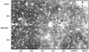 |
Fig. 1. 3 |


Log of observations of SNR 0540-69.3.
2.2. VLT observations
Further spectral observations were carried out in the 3600–6060 Å range on 2002 January 9 and 10 with the FOcal Reducer/low dispersion Spectrograph (FORS1) on the 8.2m UT3 (MELIPAL) of ESO/VLT, using the grism GRIS_600B3. This has a dispersion of 50 Å mm−1, or 1.18 Å pixel−1. The optical path also includes a Linear Atmospheric Dispersion Corrector that compensates for the effects of atmospheric dispersion (Avila et al. 1997). The spatial scale of the FORS1 CCD is 0 2 per pixel. On January 9 and 10 we obtained seven and six exposures of 1320 s each, respectively (see Table 1), that is, a total exposure time of 154 and 132 min. The position angles, PA = 88° and PA = 51°, were the same in all these exposures, and the slit positions are marked by “1” and “3” in Fig. 1, respectively.
Slits 1 (VLT) and 2 (NTT) were chosen to include the SNRC and the pulsar. Slit 3 (VLT) does not cross the SNRC, but was placed west of it, to probe the emission from the outer shell, that is most clearly identified in the Chandra X-ray images (Hwang et al. 2001, see Fig. 2). All spectroscopic observations (both NTT and VLT) were performed using a slit width of 1″, and the seeing was generally about 1″.
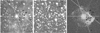 |
Fig. 2. 100″ × 100″ region of the field around 0540 marked with a box in Fig. 1. The images are obtained in the [O III]/0 (left) and [O III]/6000 (middle) bands with NTT/EMMI, and in the 1.5–6.4 keV X-ray range (right) with Chandra/ACIS (Hwang et al. 2001). The positions of all the slits used in the spectral observations, and of the detected H II regions are marked as in Fig. 1. The agreement between the optical and X-ray coordinates is subarcsecond since the pulsar was used as a reference (see Lundqvist et al. 2011). A 20″ × 20″ box marks the inner region of 0540 blown up in Fig. 4. We note that the H II structures named as “F1”, “F2”, “F4” and “F5” are projected on regions with strong X-ray emission from the SNR. |
2.3. NTT and VLT data reduction
The spatial and spectral images were bias subtracted and flat-fielded using standard procedures and utilities from the NOAO IRAF package. We used the averaged sigma clipping algorithm avsigclip with the scale parameter set equal to none to combine the images. Wavelength calibration for the 2D spectral images were done using arc frames obtained with a He/Ar lamp and procedure transform. The spectra of the objects were then extracted from the 2D image using the apall and background tasks. Flux calibration of the spectra was accomplished by comparison to the spectrophotometric standard star LTT 3864 (Hamuy et al. 1994) for both the NTT and VLT spectra. Atmospheric extinction corrections were performed using the spectroscopic extinction table atmoexan provided by ESO, and discussed in Patat et al (2011).
2.4. HST and Chandra observations
The SNR 0540-69.3 field has been imaged with the HST several times in various bands. In particular, narrow and medium band filters are useful to compare with our spectral information. The HST data highlighted here are described and discussed in Morse (2003), Morse et al. (2006) and Lundqvist et al. (2011).
To compare the optical and X-ray data, we also discuss data retrieved from the Chandra archive. In Lundqvist et al. (2011) we discuss these data in greater detail and how they were reduced.
3. Results and discussion
3.1. Imaging
Narrow-band [O III] images of 0540 obtained with NTT/EMMI through the zero velocity and +6000 km s−1 filters ([O III]/0 and [O III]/6000, respectively) are shown in the left and middle panels of Fig. 2, respectively. The FWHM of the transmission curve for both filters corresponds to 3300 km s−1 (cf. Fig. 3). The +6000 km s−1 image shows no obvious sign of [O III] emission in any part of the remnant, confirming the spectroscopic observations by Kirshner et al. (1989), who did not find any line emission with redshifts higher than ∼ 3000 km s−1. The only emission seen from the remnant in the +6000 km s−1 image is the continuum radiation from the PWN powered by the pulsar B0540-69.3 in SNRC (see Serafimovich et al. 2004; Lundqvist et al. 2011, for details on the continuum part).
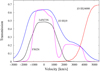 |
Fig. 3. Effective transmission curves for the ESO/[O III]/0 (blue), ESO[O III]/6000 (red) and HST/F502N (magenta) filters. The velocity is centered on the rest velocity of [O III] λ5007 in the local gas in the LMC, which we assume has a systemic shift of + 273 km s−1 compared to Earth (cf. Morse et al. 2006). The red wings of the curves ESO/[O III]/0 and HST/F502N are due to emission from [O III] λ4959 that enters the filter with a shift of ∼ 2870 km s−1. We have assumed that this line is a factor of three weaker than [O III] λ5007. The black curve shows twice the effective transmission for HST/F673N centered on [S II] λ6731, assuming the intensity of [S II] λ6716 and [S II] λ6731 to be equal. |
The zero-velocity [O III] image of Fig. 2 reveals more extended emission in accordance with Caraveo et al. (1992). Faint patchy nebulosity from the LMC background is also seen. A comparison between the [O III]/0 image and the X-ray image obtained with Chandra/ACIS (right panel of Fig. 2), where the shell-like structure associated with the outer SNR shock activity is clearly detected (Hwang et al. 2001), shows no obvious morphology that connects the optical to the X-ray emission. As seen in Fig. 2, the slits used for our spectroscopic observations encapsulate X-ray structures of the SNR. This enables us to test (see Sect. 3.3.2) whether or not optical structures projected on the regions with strong X-ray emission and named “F1”, “F2”, “F4”, and “F5” in Figs. 1 and 2 belong to, or are affected by the SNR.
The high spatial resolution of HST/WFPC2 allows us to resolve in great detail the filamentary structure of the SNRC. In Fig. 4 we present an image of this field obtained in the narrow band F673N, centered on [S II] λλ6716,6731. The F637N data, and data for the F502N band, centered on [O III] λ5007, were shown and discussed by Morse et al. (2006) and Lundqvist et al. (2011).
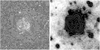 |
Fig. 4. Central 20″ × 20″ field of 0540 as viewed by HST/WFPC2/F673N (left, positive) and NTT/EMMI/[O III]/0 (right, negative). North is up and east to the left. The contours of the Chandra/ACIS X-ray fluxes in Fig. 2 are overlaid in both images. The spatial distribution of the X-ray emission shows an elongated structure with NW-SE jets, which is associated with the PWN (cf. Serafimovich et al. 2004; Lundqvist et al. 2011). As seen, the [S II] emission dominating in the HST image does not extend outside the PWN, whereas the [O III] glow in the NTT image extends far outside the PWN. |
Although detailed, the HST [S II] and [O III] narrow-band images may not fully reliably reveal the real structure and size of the SNRC. The reason is that the narrow band filters F502N and F673N may not fully cover the whole line profiles of the [O III] and [S II] emission, respectively. As shown in Morse et al. (2006), the F502N filter cuts around 5035 Å, which corresponds to ∼ + 1330 km s−1 from the rest wavelength of [O III] λ5007 (if we include a systemic shift of + 273 km s−1 for the local gas in the LMC and + 84 km s−1 for a wavelength correction for vacuum compared to air), but spectroscopic studies show (Kirshner et al. 1989, Sect. 3.2 of this paper) that the faint [O III] emission extends up to at least +1700 km s−1 (in the rest frame of LMC). This can, as pointed out by Morse et al. (2006), mean that F502N image misses out some high-velocity features of the SNRC (see also below).
The F673N filter cuts around 6770 Å, which corresponds to ∼ + 1390 km s−1 from the rest wavelength of [S II] λ6731 (for the same systemic redshift). Since the [S II] emitting region is truly more compact than that emitting [O III], also along the line of sight (Sandin et al. 2013), the F673N filter (cf. Fig. 4) should encapsulate most of the [S II] emission (see also below).
Figure 4 demonstrates the difference between the HST/WFPC2/F673N (left) and NTT/EMMI/[O III]/0 (right) images. The images are presented for the same spatial scale, and the contours of the Chandra/ACIS X-ray image are overlaid on each optical image to help us to better compare the sizes and shapes of the SNRC in both images. In the F673N image, the emission from the SNRC in the optical traces the X-ray emission, and we see no [S II] emission outside the X-ray PWN (see also Lundqvist et al. 2011).
One effect not discussed in Morse et al. (2006) is the influence of the [O III] λ4959 line on filter observations centered on [O III] λ5007. Since the velocities of the remnant are high enough for the λ4959 component to be probed by the F502N filter at velocities in the range 1900 − 4000 km s−1 (including LMC redshift), and since the expected intensity ratio Iλ5007/Iλ4959 is 3, the effective F502N filter transmission of [O III] λλ4959, 5007 looks like the magenta curve in Fig. 3. From this we can clearly see that [O III] λλ4959, 5007 is not probed well by F502N for v[O III] ≤ − 1300 km s−1, and at a redshift between 1300 − 1800 km s−1, bottoming at around 5% effective transmission at ∼ + 1500 km s−1, while emission from gas at higher velocities has about 20% effective transmission. If we compare with the velocity maps of Sandin et al. (2013) for the VIMOS/IFU field, the F502N filter mainly misses emission from gas moving away from us at projected positions ∼2″ − 3″ northeast and northwest of the pulsar, close to the pulsar, and ∼3″ southwest of the pulsar (cf. Fig. 6). As we discuss in Sect. 3.2, there are also regions outside the VIMOS/IFU field that are not probed well by the F502N filter.
The situation is different for [S II]. When both [S II] λ6716 and [S II] λ6731 are considered, Fig. 3 shows that [S II] emission is probed for the full velocity range between ∼ − 2000 km s−1 and ∼ + 2000 km s−1, with [S II] λ6716 probing the highest velocities on the red side, and [S II] λ6731 the highest velocities on the blue side. This velocity range encapsulates all [S II] emission identified by Sandin et al. (2013).
The [O III]/0 filter used in our NTT/EMMI observations has its peak transmission at 5009 Å, and has 25% transmission of the peak value at 5042 Å. Including the emission in [O III] λ4959, Fig. 3 shows that 20% effective transmission extends out to ∼ + 3500 km s−1 (including LMC redshift), without any dropouts in transmission like those of the F502N filter. The 20% transmission cutoff on the blue side of [O III] λ5007 is at ∼ − 2200 km s−1. The [O III]/0 filter is therefore likely to probe gas with all likely velocities, and with less bias than the F502N filter. Figure 3 also shows that the effective transmission is the same (19 %) for [O III]/0 and [O III]/6000 filters at ∼ 3600 km s−1, and that the [O III]/6000 filter only kicks in at velocities ≳ 3000 km s−1, which is higher than seen in spectra for [O III].
A difference image between [O III]/0 and [O III]/6000 filter observations should therefore remove stars and the synchrotron continuum from the PWN, and in principle provide a cleaner image than using HST/F502N to probe [O III]-emitting gas moving at velocities between ∼ − 2200 km s−1 and ∼ + 3000 km s−1, albeit at lower spatial resolution. We show such an image in Fig. 5. The [O III]/0 image was smoothed to match the slightly worse seeing of the [O III]/6000 image before subtraction. However, some residuals from the image subtraction remain. The surface intensity has a square root scaling to bring out faint emission. To guide the eye, we have included a circle, which corresponds to the distance freely expanding SN ejecta would reach in 1100 years if moving at 2 150 km s−1 (or in 1200 years, if moving at 1980 km s−1), and for a distance to the LMC of 50 kpc (e.g., Pietrzyński et al. 2019). Although the nebulous [O III] emission is complex, there is a hint of emission associated with the SNRC out to this radius. Figure 5 also highlights filaments F1, F2, F4, and F5.
 |
Fig. 5. 65″ × 33″ difference image between NTT/EMMI/[O III]/0 and NTT/EMMI/[O III]/6000 with square root intensity scaling to bring out faint details. The [O III]/0 image was smoothed to match the slightly worse seeing of the [O III]/6000 image before subtraction. North is up and east is to the left. The image can trace faint [O III] emission to large distances from the pulsar. A blue circle is drawn with radius 10 |

For the PWN part of the SNRC, the ground-based VIMOS/IFU [O III] images in Sandin et al. (2013), are superior to the combination of [O III]/0 and[O III]/6000, as it also adds velocity information, but those images only cover 13″ × 13″. A problem with all the mentioned methods to study the SNRC, even with the good spectral resolution of the VIMOS/IFU data, is to clean the images from [O III], and to a minor extent, He Iλ5016 (cf. Fig. 6) emission from H II regions in the LMC.
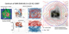 |
Fig. 6. Right: 20″ × 20″ difference image between the NTT/EMMI/[O III]/0 and NTT/EMMI/[O III]/6000 images. The blue circle has the same meaning as in Fig. 5. The flux scaling is linear. To highlight the [O III] glow, red contours are inserted for intensities up to 23% of the peak surface intensity of the PWN. Filament F1 has been marked. North is up and east to the left. Middle two top panels: [O III] λ5007 as viewed by VIMOS/IFU Sandin et al. (2013). The left of the two middle panels shows the central part, where blue is for approaching ejecta, and red for receding. A possible jet axis is highlighted for the pulsar jet. The right of the two panels brings out fainter halo emission. Middle two bottom panels: same as the two top panels, but in velocity space. A symmetry axis (also shown in the top panel) is marked that goes through rings of [O III] emitting ejecta, and the possible jet axis is highlighted for the pulsar jet (guided by Fig. 4 of Sandin et al. 2013). For the lower right panel, likely contamination from LMC H II region He Iλ5016 is marked, as is also a region with emission on the approaching side (≤ − 750 km s−1) named the blue “Wall” (also seen for [O III] λ5007 in Fig. 10). Left: Wavelet filtered HST/WFPC2/F502N map and contours of a wavelet filtered HST/WFPC2/F457M map (Lundqvist et al. 2011). Areas where the F502N fails to detect [O III] emission are highlighted. To guide the eye, a 1″ slit with PA = 90° has been drawn across all top panels. A green line in the rightmost panel marks how far west the VIMOS field reaches. All images are to scale. |
The [O III] emission in our NTT image extends outside the X-ray PWN, and the faint [O III] glow fills the space out to filament F1. This can certainly not be explained by worse spatial resolution of the ground-based observations, and further shows that we are losing some important information in the narrow band HST filters. Extended [O III] emission was discussed in Morse et al. (2006), and was traced out to a radius of ∼8″. As filament F1 lies at a projected distance of  from the pulsar, the [O III] glow is therefore more extended than argued for by Morse et al. (2006, see also below). As shown in Fig. 5, there is in particular a broad region of [O III] glow to the southwest which extends well outside the ring with a radius of 10″. We return to this below whether or not this glow is intrinsic to 0540, or emanates from other nebulae.
The [O III] glow in 0540 contrasts the situation for the Crab nebula, where the filamentary structure terminates with a shell-like structure. Observations of the filamentary ejecta in the Crab (e.g., Blair et al. 1997; Hester 1998) suggest that the filaments are the result of Rayleigh-Taylor instabilities at the interface between the synchrotron nebula and the swept-up ejecta. The emission comes from the cooling region behind the shock driven into the extended remnant by the pressure of the PWN. The same most likely applies to 0540 (cf. Williams et al. 2008, see also Sect. 3.4), but in the Crab there is no external glow (e.g., Tziamtzis et al. 2009), presumably simply because of lack of fast SN ejecta (Yang & Chevalier 2015). Further comparing with the Crab, the protruded [O III] glow in the southwestern direction in 0540, bears similarities with the Crab chimney (e.g., Rudie et al. 2008), especially when viewed through the HST/WFPC2/F502N filter (see Fig. 6).
3.2. Two-dimensional spectroscopy
As seen from Fig. 1, slits 1 and 2 cross the SNRC in two almost orthogonal directions. In both directions, the angular sizes of the SNRC are about ten times larger than the ∼1″ seeing value in our NTT and VLT spectral observations. This enables us to spectrally resolve different spatial parts of the SNRC projected on the slits, i.e., to create space-velocity maps of the encapsulated SN ejecta. In these space-velocity maps, the continuum emission was subtracted using the IRAFbackground task along the spatial axis to reveal the kinematic structure from the emission lines. We caution that the uneven LMC background introduces some uncertainty in the derived velocity structure, especially for Hα, at velocities embracing the LMC redshift, i.e., at ∼ 270 ±150 km s−1. In Fig. 6, where we include results for [O III] from Sandin et al. (2013), we have used LMC redshift as the reference velocity, and will continue to do so as default throughout the paper, unless otherwise remarked.
The slit (“slit 2”) in Fig. 7 (top panel) is oriented almost along the continuum-emitting elongated structure of the central PWN, discussed in detail by Lundqvist et al. (2011). In Fig. 7 we have used a zoomed-in and rotated version of our NTT/EMMI [O III] difference image in the right panel of Fig. 6 for reference, as this image is free from continuum sources, to show how slit 2 probes 0540.
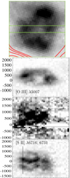 |
Fig. 7. Top panel: central 8″ × 8″ of SNR 0540-69.3 using the NTT/EMMI difference image with linear intensity scaling in Fig. 6, rotated 68° to match the horizontally marked slit 2. Lower panels: space-velocity images along slit 2 for [O III] λ5007, Hα, and [S II] λλ6716,6731. The vertical and horizontal axes show the velocity (in km s−1, corrected for the LMC redshift) and the spatial coordinate (in arcseconds) along the slit, respectively. The horizontal black lines (for Hα) mark the velocity spread of H II regions in LMC (∼ ± 125 km s−1). The velocity interval affected by the subtraction of the uneven LMC background is somewhat larger because of the finite spectral resolution. Hα is more affected by the background subtraction than other lines, and blended with [N II] λλ6548,6583. The vertical line in the [S II] image is described in Sect. 3.2. |
The second panel from the top in Fig. 7 shows the space-velocity distribution of the [O III] λ5007 emitting material encapsulated by slit 2. The space-velocity structure of [O III] λ5007 is unaffected by contamination from [O III] λ4959, which is shifted in velocity to [O III] λ5007 by 2870 km s−1.
The [O III] emission is dominated by a component with an average redshift velocity of ∼ 400 km s−1 (relative to LMC redshift). There is a slight asymmetry with the northeast part being redshifted with a few hundred km s−1 more than the southwestern part. From the 3D structure of [O III] outlined by Sandin et al. (2013), the dominating centra of [O III] emission in our space-velocity map are parts of two separate dominating ring-like structures in the ejecta. They are clearly displayed in Fig. 6.
To highlight the fainter [O III] emission, we have constructed a similar plot to that in Fig. 7, but for wider velocity and spatial ranges. This is shown in Fig. 8 where we have again used our NTT/EMMI [O III] difference image, but this time a rotated version of that in Fig. 5 to highlight fainter emission. Figure 8 also includes [O III] λ4959, which is ≈3 times fainter than [O III] λ5007, as expected. Both components of the doublet are shown to more easily evaluate high-velocity features, as well as the structure of the faint glow outside the SNRC. We have carefully subtracted stars, the PWN, and LMC H II regions to trace the weakest features. Despite this, artifacts due to over-subtraction of the LMC background emission are seen, but are not crucial to conclusions about the space-velocity structure of the [O III] glow.
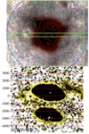 |
Fig. 8. Top panel: central 20″ × 17″ of SNR 0540-69.3 using the NTT/EMMI difference image with square root intensity scaling in Fig. 5, rotated 68° to match the horizontally marked slit 2 Bottom panel: Space-velocity image along slit 2 for [O III] λλ4959,5007. Velocity, corrected for the LMC redshift, is for [O III] λ5007. The large dynamic range of the images reveals the faint glow emission outside the SNRC of 0540. |
As seen, the faint glow has a completely different structure to that of the core, as its maximum redshift, close to + 2100 km s−1, occurs in the southwestern part, whereas the maximum blueshift, ∼ − 1300 km s−1, is in the northeastern part. The structures apparent for the two [O III] line components do not overlap, and have counterparts in both components that increase the reliability of the velocity structure. It is evident that the SNRC emission and the outer [O III] glow form two distinctly different ejecta components, which is fully consistent with the findings of Sandin et al. (2013) (see also Fig. 6), although the 3D cube of Sandin et al. (2013) did not include the highest velocities on the receding side.
We also note that the + 2100 km s−1 component has a continuation from ∼3 − 4″ southwest of the pulsar, and further along the slit in the same direction, all the way out to the edge of the frame at 9″ from the pulsar, where the glow has a velocity just redward of LMC rest velocity, but perhaps also connects to emission on the blue side. It appears as if the glow is part of an incomplete shell structure with stronger emission on the receding side to the southwest, and on the approaching side to the northeast. This is also consistent with the VIMOS/IFU image in Fig. 6. The glow continues further to the southwest, but the signal-to-noise is too low in the NTT/EMMI spectrum to trace the velocity outside the frame of Fig. 8. Signal-to-noise was also too low in the study of Mathewson et al. (1980) to probe possible broad-line emission in this direction (at PA = 60°).
Turning to [S II] λλ6716,6731 in Fig. 7, we note that it has a smaller extent to the southwest than [O III], but similar extent to the northeast. Although not shown here, we see a similarly small extent in [Ar III] λ7136. The two line components of [S II] blend together which makes the real space-velocity structure of each component more difficult to disentangle than for [O III]. In Sandin et al. (2013) we devised a way to separate the components, and at the same time create an electron density map from the relative intensities of the two [S II] line components, and we highlight this here in Sect. 3.2. The [S II] lines follow the trend for [O III] in Fig. 7, that is, there is a general redshift toward the northeast compared to the southwest. The spectral structure range between a blueshift of ∼ 800 km s−1 and a redshift of ∼ 1100 km s−1.
The Hα space-velocity structure (second panel from the bottom of Fig. 7) is less organized, mainly due to subtraction of the uneven LMC background in Hα, but there is also a hint of subtraction residuals due to [N II] λλ6548,6583. The bright emission between 700 − 1200 km s−1 actually falls on top of the [N II] λ6583 line from the LMC. Hα or [N II] was a serious matter of discussion in Kirshner et al. (1989). To underline this, there is no strong [O III] or [S II] emission just north of the pulsar along the slit reaching out to ∼ + 1900 km s−1), whereas the Hα plot shows emission there. We agree with Morse et al. (2006) that [N II] λ6583 from 0540 contributes at those wavelengths. That we expect Hα from 0540 at all mainly rests on the results from slit 1, which clearly displays several Balmer lines (see below). This was reported for the first time in Serafimovich et al. (2005), and this has led to the interpretation that 0540 stems from a Type II SN explosion with a zero-age main-sequence mass of ∼20 M⊙ (Chevalier 2006; Williams et al. 2008; Lundqvist et al. 2011).
Moving to the space-velocity diagrams for slit 1, these are shown in the images in Fig. 9. We have again used a zoomed-in and rotated (this time by 2°) version of our NTT/EMMI [O III] difference image in the right panel of Fig. 6 for reference. The [O III] λ5007 VLT/FORS image along slit 1 (Fig. 9) has a “pepper-slice”-like shape that also reflects the expansion of the SNRC. As for slit 2, the emission is heavily redshifted, but less skewed in the space-velocity diagram. The line can be traced between about − 700 km s−1 and + 1400 km s−1. It is easy to imagine a relatively symmetric (but redshifted) shell with filamentary structures reaching inward toward the center around the average velocity of the shell, i.e., ∼ 400 km s−1. However, judging from the 3D structure derived by Sandin et al. (2013) and shown in Fig. 6, the eastern and western parts of the “pepper” come from the same two ring-like features for the SNRC discussed for slit 2 above.
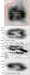 |
Fig. 9. Same as in Fig. 7, but for slit 1 (cf. Fig. 2), and for a different set of emission lines, as marked in the panels. The spatial extent of the images along the slit is 10″. As for Hα in Fig. 7, the Hβ image is corrupted by subtraction of the uneven LMC background. We note very different structures in [O II] and [O III]. |
Hβ (panel two from the bottom of Fig. 9) is partly corrupted by the LMC background subtraction, but can be seen to have a surprisingly similar structure to that of [O II] λλ3727,3729 (bottom panel of Fig. 9 in which the velocity scale is centered on 3727.5 Å). Both Hβ and the [O II] lines lack emission at the highest velocities (≳ 1200 km s−1) west of the pulsar. The different structures in [O II] and [O III] reveal different ionization conditions, especially in the western part along the slit. As a matter of fact, the [S II] 3D structure of Sandin et al. (2013) resembles those of Hβ and [O II] in Fig. 9, which may argue for that the differences between the [O III] and [S II] are more likely to be due to an effect of different levels of ionization rather than abundance effects. Moreover, the similarity between Hβ and [O II] further argues for contamination of [N II] in the Hα image in Fig. 7.
As for the NTT data in Fig. 8, the VLT data in Fig. 10 show a glow of [O III] λ5007 emission outside the inner part of the SNRC. The glow extends out to a radius of about 8″ − 10″, and seems to connect to filament F1 in the west, which in turn appears to emit at a velocity close to LMC rest velocity. The blue circle in the upper panel marks a 10″ radius from the pulsar. The space-velocity plot in Fig. 10 reveals four interesting features: fast blueshifted (at least to − 1600 km s−1) faint emission around the pulsar position, fast redshifted (at least to + 1800 km s−1) faint emission to the west of the pulsar, no redshifted emission at the pulsar position that was not already revealed by the bright emission in Fig. 9, and an intricate low-velocity structure which seems to form a loop to the east, and a stream to the west possibly connecting to regions around F1. Filament F1 itself stands out clearly, which could indicate that it is just an H II-region projected onto 0540. However, as we see in Sect. 3.4, this is not the correct interpretation. In Sect. 3.4. we also discuss [Fe III] λ4986, which would introduce emission in Fig. 10 at ∼ − 1250 km s−1. Contamination by He Iλ5016 would introduce emission at ∼ + 530 km s−1, and could be responsible for the “horn” sticking out on the eastern side in the space-velocity plot, but a similar feature is seen for [O III] λ4959, so background subtractions do not leave imprints from He Iλ5016 in Fig. 8, contrary to the VLT/VIMOS/IFU images of Sandin et al. (2013, cf. Fig. 6). We highlight that the VLT/VIMOS/IFU images neither cover F1 nor the low-velocity feature to the east.
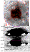 |
Fig. 10. Same as in Fig. 8, but for slit 1. The spatial extent of the images along the slit is 20″. Filament F1 is highlighted. Ellipses are drawn around [O III] λ5007, marking an ejecta velocity of + 1900 km s−1 at 4″ west of the pulsar, assuming freely coasting ejecta, and an age of 1100 years (blue) and 1200 years (red) for 0540. See text for further details. |
The impression from slit 1 is the same as from slit 2, i.e., there appears to be glow from fast [O III]-emitting ejecta with a tilt toward red on the western side and toward the blue on the eastern side. “Glow” (or at least fast [O III]-emitting ejecta) can be seen in the VIMOS/IFU image in Fig. 6 to be more pronounced for ejecta moving toward us than away from us, and this agrees with the fast blue-shifted ejecta in Fig. 10 with a projected center slightly to the east of the pulsar position.
The blue circle drawn in, for example, Fig. 10 has a radius of 10″ and corresponds to a maximum velocity of freely coasting [O III]-emitting ejecta with velocity
![Mathematical equation: $$ \begin{aligned} { v}_{\rm max}([{\text{O }}{{\small{\text{III}}}}]) = 2150\ \left(\frac{D_{\rm LMC}}{50}\right)\ \left(\frac{t_{\rm yr}}{1100}\right)^{-1} \mathrm{\,km\,s}^{-1}, \end{aligned} $$](/articles/aa/full_html/2022/02/aa41931-21/aa41931-21-eq9.gif) (1)
(1)
where DLMC is the distance to 0540 in kpc, and tyr is the age of 0540 in years. As the space-velocity spectra do not really reveal [O III] at velocities ≳ 2000 km s−1 (taking the spectral resolution into account), one may come to the conclusion that there is no support for space motions of [O III]-emitting gas much in excess of 2000 km s−1 (relative to LMC). However, for both slits 1 and 2, the maximum velocity on the red side occurs ∼4″ west and southwest of the pulsar, respectively. The true space motion of ballistic ejecta, vtrue, if originating from a central position in the SNRC, is therefore
 (2)
(2)
where robs is the projected distance from the pulsar at which the maximum observed redshift velocity, vobs, of [O III], emission occurs, and t is the age since explosion. With D = 50 kpc and robs ≈ 3.0 × 1018 cm (corresponding to 4″), one obtains vtrue([O III]) ∼ 2090(2060) km s−1 for tyr = 1100(1200) and vobs = 1900 km s−1 for slit 1, and vtrue([O III]) ∼ 2270(2240) km s−1 for tyr = 1100(1200) and vobs = 2100 km s−1 for slit 2, respectively. This is several hundred km s−1 faster than vmax([O III]) for the SNRC on the red side, and also faster than the glow on the blue side, although confusion with [O III] λ4959 causes uncertainty there.
To guide the eye, we have inserted two ellipses in Fig. 10. Both are for constant vtrue in all azimuthal directions carved out by the slit, and they are both tuned to give vobs ± 1900 km s−1 at 4″ west of the pulsar (as for slit 1). The blue and red curves are for tyr = 1100 and tyr = 1200, respectively, and DLMC = 50. Both curves encapsulate F1, but reach zero velocity at  and
and  , respectively. If vtrue is indeed the same for the full region encapsulated by the slit west of the SNRC, Figs. 5 and 10 point to an age of 1100 ≲ tyr ≲ 1200. At the position of F1 (i.e., at
  ), the red side of [O III] λ5007 should reach 800 km s−1 for tyr = 1100, and 1200 km s−1 for tyr = 1200. For a non-accelerating scenario determining vtrue (as in Eq. (2)), the pulsar seems to be significantly younger than the spin-down age, i.e., ∼1600 years. We return to the pulsar age in Sect. 3.4.3.
Looking at other parts of the space-velocity structure of the [O III] λ5007 glow for slit 1, we note that vtrue appears to be significantly lower than for the receding region west of the SNRC, perhaps except for the very eastern part, and toward the center of the SNRC on the blue side. The absence of [O III] λ5007 at high velocities on the red side toward the SNRC is remarkable, This could be due to real differences in the azimuthal distribution of [O III]-emitting gas, but it could in principle also be due to dust absorption screening off the red side behind the SNRC. We find this explanation less likely though, since the dust would have to be located between the SNRC and fast (unseen due to dust) ejecta on the blue side, while there is no dust counterpart on the approaching side. Moreover, one does not see this effect in the Crab, despite it containing large amounts of dust (Gomez et al. 2012). In the Crab the dust is concentrated to filaments with modest filling factor, which in the optical are notably strong in [O III].
The picture that emerges for the [O III] glow, seen through slits 1 and 2, is that it does not come from a spherically symmetric shell surrounding the SNRC, but from a much less complete structure. On the blue side it appears to be concentrated to the “wall”-like structure centered just west of the pulsar position and reaching out to ∼ − 1600 km s−1 seen and marked as “Blue Wall” in Fig. 6, and shown by Sandin et al. (2013). On the red side, the fastest glow is in the southwestern and western parts ∼4″ from the pulsar reaching space velocities well in excess of 2000 km s−1. In the eastern part, velocities covered by slits 1 and 2 are less extreme, especially on the receding side. However, our slits do not cover the southeastern part. Here we make use of the long-slit observations by Morse et al. (2006) (described more in Sect. 3.3.1) as they cover the southeastern and northwestern parts of the [O III] glow region. Figure 5a of Morse et al. (2006) shows a clear asymmetry for the [O III] glow not covered by our slits 1 and 2, or the VIMOS/IFU data of Sandin et al. (2013). The figure of Morse et al. (2006) shows strong [O III] glow on the approaching side to the northwest, as well to the southeast for the receding side. Apart from the “wall”-like structure on the blue side (which is also evident as the blue-ward emission in the VIMOS/IFU spectrum in Fig. 19), it appears as if the incomplete shell of [O III] glow is devoid of emission on the receding northern side, and on the approaching southern side.
The two components of the [S II] doublet in Fig. 7 have a difference in wavelength corresponding to a velocity shift of ≈ 640 km s−1. In 0540 they blend together because of the velocity broadening of the emitting gas. There are, however, a few positions along the slit for which the blend is small. One such position is marked with a vertical solid line in Fig. 7, along detector row 29 in our notation. We discussed the deblending of [S II] λλ6716,6731 along this row in Serafimovich et al. (2005), assuming that the line intensity ratio ![Mathematical equation: $ R_{[{\mathrm{S}\,\small{\text{II}}}]} = \frac{I(\lambda6716)}{I(\lambda6731)} $](/articles/aa/full_html/2022/02/aa41931-21/aa41931-21-eq14.gif) is the same for all parts of the supernova remnant encapsulated by the slit row. As R[S II] is density sensitive (e.g., Osterbrock & Ferland 2006), we effectively assumed that the density is constant in this part of the remnant. The deblendig in Serafimovich et al. (2005) resulted in R[S II] = 0.7, and the multilevel model for [S II] described in Maran et al. (2000) was used to obtain ne(1.4 − 4.3) × 103 cm−3 for the temperature T = 104 K, and ne = (1.8 − 5.3) × 103 cm−3 for T = 2 × 10⁴ K.
is the same for all parts of the supernova remnant encapsulated by the slit row. As R[S II] is density sensitive (e.g., Osterbrock & Ferland 2006), we effectively assumed that the density is constant in this part of the remnant. The deblendig in Serafimovich et al. (2005) resulted in R[S II] = 0.7, and the multilevel model for [S II] described in Maran et al. (2000) was used to obtain ne(1.4 − 4.3) × 103 cm−3 for the temperature T = 104 K, and ne = (1.8 − 5.3) × 103 cm−3 for T = 2 × 10⁴ K.
As we discuss in Sect. 3.4, the temperature in the [S II]-emitting gas is probably T ∼ 15 000 K. In addition, a more careful background subtraction along row 29 than the preliminary one in Serafimovich et al. (2005) gives R[S II] = 0.85 ± 0.10, translating into ne = (0.9 − 2.0) × 103 cm−3. This is fully consistent with densities found in the Crab Nebula for which [O II] and [S II] line ratios indicate electron densities in the range 4 × 10² − 4 × 103 cm−3 for the various filaments observed (Davidson & Fesen 1985). For the region mapped out by our detector row 29, Sandin et al. (2013) estimate ne ≲ 1 × 103 cm−3. As emphasized by these authors there are, however, pockets of ejecta with ne ∼ (1 − 2) × 103 cm−3 in the SNRC when spectra from individual fibers are studied; their density plot was smoothed over a 2 × 2 pixel kernel. Inspection of the individual fiber spectra of Sandin et al. (2013) also reveals background LMC residuals, which introduces a bias to underestimate electron densities from [S II]. The reason is the small field of view of VIMOS, which makes background subtraction cumbersome. Our estimate of ne ∼ (1 − 2) × 103 cm−3 for detector row 29 are therefore not in conflict with Sandin et al. (2013). For a more complete discussion about the variation of electron density from [S II] within the SNRC, we refer to Sandin et al. (2013), with the caveat in mind that the electron densities in that paper could be somewhat underestimated in general. In addition, we emphasize that the densities derived for detector row 29, and in Sandin et al. (2013), are average densities along the line-of-sight for the SNRC, unlike the situation in the Crab, for which more detailed 3D studies can be done more easily, due its proximity (e.g., Charlebois et al. 2010; Martin et al. 2021). In the analysis in Sect. 3.4 for the SNRC, we use ne = 103 cm−3 unless otherwise specified.
3.3. One-dimensional spectroscopy
3.3.1. The central part of 0540
Previous optical spectroscopic studies of the SNRC were carried out by Mathewson et al. (1980), Kirshner et al. (1989) and Morse et al. (2006), and we reported preliminary results of our NTT/EMMI and VLT/FORS observations in Serafimovich et al. (2005). We mainly compare with Kirshner et al. (1989) and Morse et al. (2006). Kirshner et al. (1989) used a slightly larger slit ( ) than us, and positioned their slit to cross the SNRC at PA = 77°. Morse et al. (2006) used an even wider slit (2″) at PA = 124°, and we discussed some of their results already in Sect. 3.2.
We extracted 1D spectra of the SNRC from our spectral images using the IRAF procedure apall, and spatial extents of 10″ and 8″ centered on the pulsar for slits “1” and “2”, respectively. The extracted windows correspond to the observed extents of the SNRC along the respective slit directions. The extracted spectra are shown in Figs. 11 and 12.
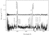 |
Fig. 11. Spectrum of the central part of the SNR 0540-69.3 obtained with ESO/NTT (PA = 22°). The lower panel has an expanded flux scale to highlight weaker lines. The spectrum has been dereddened using E(B − V) = 0.19 and RV = 3.1. “Hα” is a blend of Hα and [N II] λλ6548,6583. |
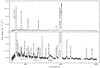 |
Fig. 12. Spectrum obtained with ESO/VLT (PA = 88°), and again (as in the Fig. 11) the lower panel is plotted to bring out weaker lines. The spectrum has been dereddened using E(B − V) = 0.19 and RV = 3.1. We note the significantly higher signal-to-noise in the VLT spectrum compared to Fig. 11, which made it possible to detect new lines in SNR 0540-69.3 as reported in Serafimovich et al. (2005) and here. Of particular importance are the [Ne III] lines and Hβ (see text). |
Line fluxes were derived by integrating over each line profile. (No Gausian fitting can be done since the line profiles are strongly non-Gaussian.) This gives accurate fluxes for strong lines like [O II] and [O III], as found from a test where we varied the background level up and down by 1σ from the mean value; the statistical error of the strongest lines is less than 5%. For faint lines, like the [Fe II] lines and Mg I], the flux uncertainty can be up to 40%. In Table 2, we have marked the fluxes of such lines by a colon.
Dereddened line fluxes relative to [O III] λ5007 and line velocities in SNR 0540-69.3.
A list of identified lines and their measured fluxes, central wavelengths, and velocities, is presented in Table 2. The results of Kirshner et al. (1989) and Morse et al. (2006) are also included for comparison. All our fluxes have been dereddened using E(B − V) = 0.19 and RV = 3.1, as was also done by Kirshner et al., while Morse et al. (2006) used E(B − V) = 0.20. A detailed discussion on the extinction toward 0540 can be found in Serafimovich et al. (2004). From that discussion, we highlight that the uncertainty in line ratios for 0540 for the optical range, due to uncertainty in extinction, should be small (≲5%).
Our fluxes were normalized to [O III] λ5007. We note that Kirshner et al. (1989) and Morse et al. (2006) normalized to the sum of [O III] λ4959 and [O III] λ5007. In Table 2, we therefore simply assumed a 1 : 3 line ratio for those two components, and renormalized all fluxes in Kirshner et al. (1989) and Morse et al. (2006) to [O III] λ5007. Guided by the VIMOS/IFU observations of Sandin et al. (2013), who concentrated on the two doublets [O III] λλ4959, 5007 and [S II] λλ6716, 6731, one expects line fluxes for the various slit orientations shown in Table 2 to be different, just because of different parts of the SNRC being caught by the slits.
Our 1D spectra of the SNRC are consistent with those of the other studies, but also reveal many differences. The higher sensitivity of the VLT observations allowed us in Serafimovich et al. (2005) to report many new lines not detected in previous studies, and we report more here. The most important findings in Serafimovich et al. (2005) were [Ne III] λλ3869,3967 and Balmer lines of hydrogen all the way down to H Iλ3889 (Hζ). While the neon lines constrain the supernova, the Balmer lines show that the previously detected emission around Hα is at least partly due to Hα, and not only to [N II] λ6583, or any other line as discussed by Caraveo et al. (1998). We do not try to separate Hα from [N II] λλ6548,6583. However, from the Hα panel of Fig. 7 it is clear that [N II] is present with a velocity structure that looks similar to that of [S II], and with a velocity for [N II] λ6583 that reaches at least + 1000 km s−1 in the LMC rest frame. Morse et al. (2006) estimated an intensity ratio of IHα/IN II] ∼ 1.1 for their slit position.
The [Ne III] λλ3869,3967 lines, and [O III] λ4363 are all contaminated by H I lines, which leads to an overestimate of the fluxes of these lines, neither accounted for in Table 2, nor for [O III] λ4363 fluxes in previous investigations. Another complication is that all H I lines suffer from influence of the uneven LMC background which must be compensated for. We discuss this further Sect. 3.4.
Using unblended lines we estimate that the mean velocity of the central region of the 0540 system is +500 ± 55 km s−1 for slit “1” and +380 ± 60 km s−1 for slit “2”, respectively, when the LMC redshift of 270 km s−1 is accounted for. Within errors both values are consistent with each other, and a mean velocity of the two gives +440 ± 80 km s−1. This is ∼ 100 km s−1 higher than the value of Kirshner et al. (1989), but the two investigations are consistent with each other, despite different slit orientations.
The redshift of the SNRC of 0540 is indeed large. An explanation could be that the 0540 system is the result of an asymmetric explosion, as discussed by Serafimovich et al. (2004). The SNRC of 0540 is not unique in that sense. Balick & Heckman (1978) found that the oxygen-rich SNR NGC 4449 also moves at a velocity of ∼ 500 km s−1 relative to its surrounding H II regions. As for 0540, this remnant is also oxygen-rich. Over a larger scale, 0540 may not be all that asymmetric, as revealed by the [O III] glow from ejecta moving at high speed (≳ 1500 km s−1) both toward and away from us discussed in Sect. 3.2. (see also Morse et al. 2006; Sandin et al. 2013).
3.3.2. Filaments
SNR 0540-69.3 is near the LMC H II region DEM 269 and the OB association LH 104 (see Kirshner et al. 1989, and references therein, as well as below). This is consistent with that we detect narrow emission lines that vary spatially in strength along our slits. The lines are spectrally unresolved (except for one case, see below).
To study whether or not some of these emitting regions are affected by the SNR activity, we looked at filaments detected along the slits. We mainly considered those with an [O III] temperature in clear excess of 104 K, as is usually observed in shocks or photoionization heated regions of known SNRs. We assumed the same extinction for the filaments as for the remnant, and used the standard ratio ![Mathematical equation: $ R_{[{\mathrm{O}\,\small{\text{III}}}]} = \frac{I(\lambda4959)+I(\lambda5007)}{I(\lambda4363)} $](/articles/aa/full_html/2022/02/aa41931-21/aa41931-21-eq16.gif) for the temperature (e.g., Osterbrock & Ferland 2006). We also looked for lines of highly ionized ions as tracers of influence by the SNR. We detected a few filaments of interest along the VLT slits “1” and “3”, and they are marked as F1, F2, F4, and F5 in Fig. 1. We also mark filament F3, and use this as reference for a presumed LMC H II region.
for the temperature (e.g., Osterbrock & Ferland 2006). We also looked for lines of highly ionized ions as tracers of influence by the SNR. We detected a few filaments of interest along the VLT slits “1” and “3”, and they are marked as F1, F2, F4, and F5 in Fig. 1. We also mark filament F3, and use this as reference for a presumed LMC H II region.
The typical size of the filaments along the slit is ∼3″. As in the case of the SNRC, we have constructed 1D spectra for each filament. The dereddened spectra of F1, which is closest to the SNRC in projection, and F5, which appears close to the outer shock front detected in X-rays, are shown in Figs. 13 and 14, respectively. Spectra of the other filaments are similar to the ones presented. Lists of identified spectral lines for F1-F5 with measured fluxes, central wavelengths, and velocities, are presented in Tables 3 and 4. We return to a more detailed discussion of the filaments in Sect. 3.4.3.
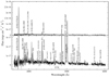 |
Fig. 13. Spectrum of filament F1 in the vicinity of SNR 0540-69.3. The filament is situated only 8″ west of the pulsar (see Figs. 1 and 2). As in Figs. 11 and 12, we have also plotted the spectra with expanded flux scales to highlight weaker lines. The spectrum was dereddened using E(B − V) = 0.19 and RV = 3.1. We note that the broad base of the [O III] λλ4959,5007 lines is skewed to the red as compared to the narrow components, reaching at least +1700 km s−1. No such features are seen in spectra of the emission from filaments F2, F3, F4, or F5 (see Fig. 14), as marked in Fig. 1. Line fluxes of all filaments are given in Tables 3 and 4. |
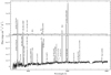 |
Fig. 14. Spectrum of an H II region along the VLT slit “3” at a projected distance of 25″ to the west of the pulsar (called filament F5 in Figs. 1 and 2). As in Fig. 11, we have also plotted spectra with expanded flux scales to highlight weaker lines. The spectrum have been dereddened using E(B − V) = 0.19 and RV = 3.1. |
Dereddened line fluxes relative to Hβ and line velocity in H II regions along the VLT “slit 1”.
Dereddened line fluxes relative to Hβ and line velocities in H II regions along the VLT “slit 3”.
3.4. Line profiles and intensities
3.4.1. The central part
Supernova remnants are good laboratories to test the theory of stellar evolution, explosive nucleosynthesis, radiation processes, and shock physics. To test the first two items, an estimate of elemental abundances of the ejecta is essential. As the information from SNRs mainly rests on collisionally excited lines, we therefore also require knowledge about the density and temperature of the emitting gas.
The observed strength of the spectral lines allow us to deduce this information. The prime thermometer is R[O III]. Because we see [O III] λλ4959, 5007 and [O III] λ4363 in all VLT spectra of 0540 and the filaments, we are able to estimate the temperature of the [O III] emitting plasma in both the SN ejecta and the filaments.
Unfortunately, for the SNRC with its broade lines, [O III] λ4363 is blended with Hγ. This may lead to over-estimating the [O III] temperature. To get the real [O III] temperature, we subtracted Hγ from the line profile of the observed [O III] λ4363+Hγ blend. As a template profile for all H I lines we used Hβ. As shown in Fig. 15, the Hβ template is affected by [Fe III] λ4481, but this has very small impact on the process of removing the bluer Balmer lines. A further complication is that all hydrogen lines suffer from background contamination of emission around LMC rest velocity. We approximated this for all H I lines by a linear approximation of the flux across the corrupted frequency range.
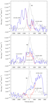 |
Fig. 15. Line profiles of the Balmer lines from 0540 in velocity space relative to LMC for the VLT spectrum in Fig. 12. Top panel: Hζ blended with [Ne III] λ3869, middle panel: Hϵ blended with [Ne III] λ3967, and bottom panel: Hγ blended with [O III] λ4363. In all panels we also show Hβ (gray) and the continuum level (black). Hβ was used as a template to subtract the expected emission from Hγ, Hϵ and Hζ using Case B line ratios (Brocklehurst 1971). The blue and red solid lines show [O III] λ4363 and [Ne III] λλ3869,3967 before and after deblending, respectively. |
The expected flux of Hγ relative to Hβ was estimated from Case B theory (Brocklehurst 1971). The bottom panel of Fig. 15 shows how we were able to remove Hγ from the [O III] λ4363+Hγ blend. As a spin-off, the line subtraction confirms the values we used for the dereddening, i.e., E(B − V) = 0.19 and RV = 3.1; when the Balmer line was removed, continuum level was attained.
After the Hγ subtraction, the flux of [O III] λ4363 relative to [O III] λ5007 (set to 100) is ∼4.3 (instead of 5.7, if Hγ is unaccounted for). This gives R[O III] ∼ 31. We can, however, refine this analysis by comparing the deblended profile of [O III] λ4363 to that of a template profile for [O III] λλ4959,5007. The template for the latter was made from a similar procedure to what was done in Sandin et al. (2013), that is, the blue part of [O III] λ4959 and the red part of [O III] λ5007 were used as initial guesses for the template. With the known intensity ratio of 3 for I(λ5007)/I(λ4959), we constructed the combined [O III] λλ4959,5007 template shown in red in Fig. 16. The template is for the sum of the two line components. In the same figure we have also included the “clean” [O III] λ4363 profile from Fig. 15. Once multiplied by a factor of 28, and once by 34. In general, the [O III] λ4363 profile is similar to that of the [O III] λλ4959,5007 template, although noise limits the usefulness of the [O III] λ4363 profile in its wings.
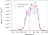 |
Fig. 16. Line profiles of [O III] λλ4959,5007 and [O III] λ4363 of the emission from 0540 as observed through the VLT slit. The velocity is relative to LMC. The [O III] λλ4959,5007 profile was created from a cleaning procedure described in the text, and is for the sum of the two line components. The [O III] λ4363 is the blue-red profile in the bottom panel of Fig. 15. The flux of [O III] λ4363 has been multiplied by 28 and 34 to match the various parts of the line profiles. There is a tendency of relatively weaker [O III] λ4363 emission on the blue side, which could mean hotter [O III]-emitting plasma on the receding side of 0540 (see text). |
We thus find R[O III] = 31 ± 3, with a tendency for a lower ratio in the blue part of the line profile compared to the red. The corresponding [O III] temperature range for the SNRC is 23 500 ± 1800 K (cf. Table 5). This is less than ∼34 000 K, but consistent with ≈25 500 K estimated by Kirshner et al. (1989) and Morse et al. (2006), resepctively. In neither of those two studies Hγ was accounted for. The slightly larger ratio we find for R[O III] for the receding side of the remnant (compared to LMC rest velocity) could be due to a lower temperature in this part of the SNRC, or intrinsic dust reddening. The latter would not be surprising considering that dust in the Crab nebula is concentrated to [O III]-emitting filaments, and the pathlength through dust to the receding side of the SNRC is likely to be longer than to ejecta moving toward us. To compensate for the factor ∼1.2 larger R[O III]-value for the red side, E(B − V) would have to be ∼0.5 instead of 0.19. This would depress the red side of the line profiles severely, which is not what we see. Dust is therefore not a likely reason for the large R[O III]-value on the red side of the [O III] lines.
Figure 16 shows that the blue sides of [O III] λ4959 and [O III] λ5007 nearly reach − 1900 km s−1, which was difficult to disentangle from Fig. 10 due to blending. For the red side, the maximum velocity is + 1700 km s−1, which is consistent with the space-velocity results. Figure 17 shows that the construction of the [O III] λλ4959,5007 template reveals a residual that we attribute to [Fe III] λ4986, a line that is also seen in the spectra of the filaments and other SNRs (Fesen & Hurford 1996).
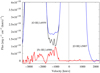 |
Fig. 17. Sum of the “cleaned” [O III]λλ4959,5007 profiles (cf. Fig. 16) of the emission from 0540 (black) compared to the observed emission (blue). The velocity scale is for the λ5007 component relative to LMC. The difference (red) is attributed to [Fe III] λ4986. The maximum velocity on the red side of [O III] λ5007 is ≈ + 1800 km s−1, which may be less than on the blue side (≈ − 1900 km s−1, see Fig. 16). |
The [Ne III] λλ3869,3967 doublet is also affected by blending with Balmer lines. The same subtraction routine was applied for both components of [Ne III], and in Fig. 15 we show how the Balmer lines Hζ and Hϵ were removed from their blends with [Ne III] λ3869 and [Ne III] λ3968, respectively. As seen from the figure, [Ne III] λ3869 is insignificantly contaminated by Balmer line emission, whereas [Ne III] λ3967 is more affected.
A direct comparison between [Ne III] λ3869 and [O III] λ5007 is shown in Fig. 18. The profile of the neon line is fairly noisy, but it is consistent with the general features and maximum velocities of [O III] λ5007. The ratio of the two lines is I[O III] λ5007/I[Ne III] λ3869 ∼ 30. With a temperature of 23 500 ± 1800 K, and assuming similar ionization structures of O2+ and Ne2+, our multilevel atom models (e.g., Maran et al. 2000; Mattila et al. 2010), updated with the recent atomic data in the CHIANTI database (Del Zanna et al. 2021), result in a mass ratio MNe/MO ∼ 0.07, which should probably be considered a lower limit since the ionization zone of O2+ is likely to be wider than that of Ne2+. In this context, we highlight the observations of Morse et al. (2006). They detected [Ne III] λ3869, but neither got a 3σ detection of [Ne III] λ3967, nor corrected for Balmer line contamination. Their flux values translate into MNe/MO ∼ 0.13 for the temperature we find from [O III].
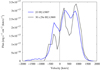 |
Fig. 18. Same profile for [O III] as in Fig. 16, but only for [O III] λ5007 (blue) together with the “cleaned” [Ne III] λ3869 profile in Fig. 15. The [Ne III] profile was multiplied by a factor of 30 to match [O III] λ5007. We note similar widths and structures of the two profiles. Noise is too high for the [Ne III] line to trace it out the highest velocities on the blue side. |
Williams et al. (2008) modeled the emission from 0540, and in those models they assumed the abundance ratio Ne/O = 0.2 (i.e., a mass ratio of 0.25), and obtained I[Ne III] λ3869/I[O III] λ5007 = 0.093. This is almost three times the value we obtain from our observations; if the MNe/MO ratio in their model is lowered to 0.085 (i.e., close to our value of 0.07), their predicted line ratio should agree with our observations. The question is how likely a value of MNe/MO ∼ 0.1 could be. It is, for example, about half the mass ratio for the inner ejecta found in a recent model for the nucleosynthesis yields for the central part of an exploding 11.8 M⊙ star (Sieverding et al. 2020), but the models of Chieffi & Limongi (2013), which take rotation of the progenitor into account, yield MNe/MO = 0.063 (0.053) (0.21) M⊙ for progenitor masses of 13 (15) (20) M⊙. For nonrotating progenitors Chieffi & Limongi (2013) find MNe/MO = 0.22 (0.46) (0.32) M⊙. Judging from this, rotation could be important as MNe/MO in those models agree with the values derived from observations.
In the models of Williams et al. (2008), infrared lines observed with the Spitzer Space Telescope were included. To compare the IR lines to optical lines, these authors multiplied the fluxes in Morse et al. (2006) by a factor of 4 to account for the 2″ slit in the optical as the infrared observations observed the full region. We use the same procedure, but to put the slit compensation on firmer footing, we make use of the VLT/VIMOS observations of Sandin et al. (2013). In Fig. 19 we show the line profile of [O III] λ5007 for the full 13″ × 13″ field observed with VIMOS, and compare this to 7.2× the template [O III] λ5007 profile from our slit 1 observations. With the 7.2 factor, the integrated emission of the two profiles is the same for velocities ≳ − 750 km s−1. About 10% of the VIMOS [O III] λ5007 flux falls at velocities below − 750 km s−1, and is mainly attributed to [O III] glow not captured efficiently by the slits used by Morse et al. (2006) and us. We therefore use the factor of 7.2 for most lines For lines with suspected glow we use 8.0, since the Spitzer field-of-view is likely to capture much of the glow. (The corresponding numbers for our NTT/EMMI slit, i.e., slit 2, is 6.3 and 6.6, respectively.) As Morse et al. (2006) obtain ≈1.6 times larger [O III] λ5007 flux through their 2″ × 11″ slit than we do through our 1″ × 10″ slit, the conversion factor Williams et al. (2008) should have used for most lines is 4.5, instead of their 4. For [O III] λ5007, and other possible lines with glow, a conversion factor of 5 would have been more appropriate.
 |
Fig. 19. Same profile for [O III]λλ4959,5007 as in Fig. 16 (blue), together with the [O III]λλ4959,5007 profile for the full 13″ × 13″ field as observed by Sandin et al. (2013). The slit 1 profile was multiplied by a factor of 7.2 to match the integrated emission at ≥ − 750 km s−1. We note strong [O III] emission for ≤ − 750 km s−1 for the larger field-of-view compared to the slit 1 observations. This emission corresponds to about 10% of the total [O III] emission. A minor fraction (∼10%) of the emission at ≤ − 750 km s−1 could be due to [Fe III] λ4986, as displayed in Fig. 17, but most of it comes from the approaching “wall” described in Sect. 3.2. |
Williams et al. (2008) measure (7.29 ± 0.56)×10−14 erg cm−2 s−1 for [Ne III] 15.6μ. If we use our VLT observations, multiplied by 8, the [Ne III] λ3869 flux is 1.1 × 10⁻¹⁴ erg cm−2 s−1, i.e., I[Ne III] 15.6μ/I[Ne III] λ3869 ∼ 6.7, which is twice as high as in the model of Williams et al. (2008). From our multilevel modeling it is obvious that the [Ne III] 15.6μ flux cannot come from the same hot gas as the [O III] lines we observe, since the ratio for this at 23 000 K is I[Ne III] 15.6μ/I[Ne III] λ3869 ∼ 0.14. An intensity ratio of 6.7 is only obtained for temperatures ≲7000 K. Although there are several uncertainties, the main explanation must be that [Ne III] 15.6μ predominantly comes from regions with much lower temperatures than that emitting the optical [O III] and [Ne III] lines. The most likely region is gas heated by photionization rather than by shocks, as shock-heated material would be hotter. Extinction due to internal dust may be a complementary explanation as this would not affect the IR line.
Figure 19 emphasizes the redshift of all [O III] emission from the full SNRC, and shows that the line profile through slit 1 surprisingly well represents the emission at most velocities. The most obvious difference is the strong emission at velocities ≲ − 750 km s−1 (which is also evident from Fig. 6, and which is mainly due to the approaching “wall” described in Sect. 3.2) as well as slightly more emission at ≳ + 750 km s−1. The peak around LMC rest velocity is at least to some extent artificial due to difficulty with removing LMC background emission due to the small field-of-view of VIMOS. The VIMOS data are not sensitive enough to trace velocities ≳ ∣±1500∣ km s−1.
Turning to ions of lower degree of ionization observed through slit 1, we show [O II] λλ3726,3729 in Fig. 20, [S II] λλ4069,4076 in Fig. 21, and He Iλ5876 in Fig. 22. For [O II] and [S II] we have centered the velocity on 3727.5 Å and the strongest component of [S II] (i.e., λ4069), respectively. As already discussed in Sect. 3.2, [O II] has a profile similar to that of Hβ, and [S II] λλ4069,4076 is similarly narrow, that is, primarily extends from ∼ − 700 km s−1 to ∼ + 1000 km s−1, although there is a blue wing of [O II] that reaches ∼ − 1400 km s−1. This is not seen for [S II] λλ4069,4076 in Fig. 21, but the low signal-to-noise does not allow us to draw firm conclusions on that part of the line profile. Interestingly enough, the full view SNRC observations in [S II] λλ6716,6731 by Sandin et al. (2013, their Fig. 2) does show a blue wing between − 1200 km s−1 and − 700 km s−1. Our choice to center the [O II] doublet on 3727.5 Å is because this does not introduce any bias for either of the two doublet components. What is intrinsically assumed by centering on 3727.5 Å is that we assume that I[O II] λ3729/I[O II] λ3726 ≈ 1.11, which means ne ∼ 350(400) cm−3 for T ∼ 20 000 (30 000) K. According to our multilevel model, the intensity ratio decreases from ≈1.35 to ≈0.38, as electron density increases from 102 cm−3 to 104 cm−3.
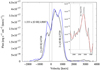 |
Fig. 20. Same profile for [O III]λλ4959,5007 as in Fig. 16 (blue), together with the combined [O II] λλ3726,3729 profile. The velocity for the [O II] lines is centered on 3727.5 Å. The [O II] profile was multiplied by a factor of 2 to match 1.33× [O III] λ5007. We note that [O II] λ3726 only reaches ≈ − 1400 km s−1 on the blue side (when the 118 km s−1 difference between [O II] λ3726 and 3727.5 Å is accounted for). On the red side of [O II] λ3729 the emission is blended with [Fe VII] λ3759, as shown by the inset. The red curve is Savitzky-Golay fitting to the noisy [Fe VII] line profile. |
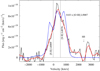 |
Fig. 21. Same as in Fig. 18, but for [S II] λλ4069,4076 (black, and smoothed in red) instead of [Ne III] λ3869. The [O IIII] profile was multiplied by a factor of 0.03 to match [S II]. The sulfur doublet was velocity-centered on the λ4069 component. LMC rest frame velocities for both components are marked by vertical thin lines. The red side of the [S II] doublet is affected by Hδ. (The dip in Hδ is due to over-subtraction of the LMC background.) |
Our observed I[S II] λλ4069,4076/I[O II] λλ3726,3729 ratio is ∼0.06. For the temperature interval 10 000 − 15 000 K, and density interval 500 − 1000 cm−3, our multilevel model atoms translate the observed ratio into an abundance ratio of S/O = 0.05 ± 0.01, and thus a mass ratio MS/MO = 0.10 ± 0.02. The models of Chieffi & Limongi (2013) predict a ratio of 0.05 − 0.06 for rotating progenitors for progenitor masses between 13 − 20 M⊙, and between 0.05 − 0.13 for nonrotating (with 0.05 for 20 M⊙). The more recent model of Sieverding et al. (2020) predicts MS/MO = 0.085 from their 11.8 M⊙ model for the inner ejecta, and 0.12 M⊙ for all ejecta. Williams et al. (2008) assumed MS/MO = 0.05 in their models, and underproduced [S III] 18μ and [S IV] 10μ by factors of ∼1.4 and ∼2.8, respectively, when we adjust their results with more accurate slit compensations. It therefore appears as if their model would fit the Spitzer data better with MS/MO ∼ 0.1, which is consistent with both Chieffi & Limongi (2013) and Sieverding et al. (2020), albeit perhaps not for nonrotating low-mass progenitors in the case of Chieffi & Limongi (2013). However, the model of Williams et al. (2008) gives an I[S II] λλ4069,4076/I[O II] λλ3726,3729 ratio which is ∼0.09, and that is on the high side compared to our observations already with MS/MO = 0.05.
The ratio MS/MO can also be estimated from our slit 2 data, for which we have I[S II] λλ6716,6731/I[O II] λλ7319−7331 ∼ 9.0. This is similar to ≈8.4 by Kirshner et al. (1989), and 10 in the model of Williams et al. (2008) assuming S/O = 0.1). Our multilevel atom modeling shows that a temperature ≳20 000 K is needed to excite O+ to emit [O II] λλ7319-7331 at the observed relative intensity. In particular, for the [O III] temperature T ∼ 23 000 K, I[S II] λλ6716,6731/I[O II] λλ7319−7331 ∼ 7 for S/O = 0.1 and electron densities estimated by Sandin et al. (2013). The ratio rises steeply below 20 000 K.
Another way to estimate a temperature in the [O II]-emitting regions is from the ratio I[O II] λλ3726,3729/I[O II] λλ7319−7331, but for this we have to combine slits 1 and 2. Using the slit correction factors 7.2 and 6.3, respectively, we obtain ∼6.2, which is very close to ∼6.5 by Kirshner et al. (1989), but very different from the modeled flux by Williams et al. (2008), which is ≈14.7. Our multilevel model suggests very high temperatures (well above 30 000 K) to get a ratio below 8.0, which appears unlikely. Since our flux agrees with that of Kirshner et al. (1989), a possible explanation could be that [O II] λλ7319−7331 is contaminated by [Ca II] in both our slit 2 and the data in Williams et al. (2008). Such contamination (at 20% level) was already discussed by Kirshner et al. (1989).
A combination of slits 1 and 2 can also be used to estimate an [S II]- temperature from I[S II] λλ6716,6731/I[S II] λλ4069,4076, which with our slit compensations is ∼30. This is much higher than ∼17 by Kirshner et al. (1989), and inconsistent with ∼9.4 by Morse et al. (2006), as well as the model by Williams et al. (2008) which predicts ∼7.4. Our multilevel models show some density dependence, but intensity ratios such as those by Morse et al. (2006) and Williams et al. (2008) require temperatures at least as high as our derived [O III] temperature from slit 1, whereas our ratio and that of Kirshner et al. (1989) indicate temperatures of well below 10 000 K and around 15 000 K, respectively. Comparing observations through different slits, and at different epochs, admittedly increases the risk of systematic errors, so to make a consistency check we have used the full SNRC [S II] spectra of Sandin et al. (2013) to make artificial observations of [S II] through slits 1 and 2. From this exercise, we find that the slit compensation for [S II] λλ6716,6731 is 6.5 for slit 1 and 7.7 for slit 2 (instead of the values 7.2 and 6.3, as indicated by [O III]). This is not large enough to change our I[S II] λλ6716,6731/I[S II] λλ4069,4076 ratio by much (and actually makes it even larger).
The source of inconsistency for I[S II] λλ6716,6731/I[S II] λλ4069,4076 could either lie in the large relative [S II] λλ6716,6731 flux we get for slit 2 compared to others (cf. Table 2), and/or the lower flux we measure for [S II] λλ4069,4076. The latter is not unreasonable since [S II] λλ4069,4076 is affected by Hδ. From Brocklehurst (1971) we estimate that Hδ would amount to ∼25% of Hβ, which would decrease the I[S II] λλ6716,6731/I[S II] λλ4069,4076 ratio accordingly, if not corrected for. This effect, of course, does not affect the modeled results of Williams et al. (2008). Regarding [S II] λλ6716,6731 we can do a direct test against the VIMOS observations of Sandin et al. (2013) by placing artificial slits on the VIMOS images to simulate slits 1 and 2. From Fig. 3 of Sandin et al. (2013) it can be seen that I[S II] λλ6716,6731/I[O III] λ5007 is never higher than ∼0.8, and for slits 1 and 2 we get ∼0.47 and ∼0.35, respectively. Even if we allow for slight displacement of slit 2 due to atmospheric dispersion (which was not accounted for in the NTT/EMMI observations), the ratio will not increase by more than ∼20%. Careful check of possible erroneous background subtraction of [S II] λλ6716,6731, together with the fact that the flux of other lines through slit 2 agrees with the results of Kirshner et al. (1989) and Morse et al. (2006), leaves us no choice other than to suggest that the [S II] λλ6716,6731 flux could vary with time. If we use a ratio of 0.35 from a simulated slit 2, we obtain I[S II] λλ6716,6731/I[S II] λλ4069,4076 ∼ 12, which is more aligned with what other groups get, and would suggest an [S II] temperature of ∼20 000 K. The question remains regarding our high [S II] λλ6716,6731 flux. We note that there are NTTT/EMMI spectra covering [S II] λλ6716,6731 from 1995 January, that is, only one year before our NTT spectrum, which were shown in Caraveo et al. (1998). Unfortunately, these authors did not provide any fluxes. As there is activity going on in the southwestern part of the PWN, at least between 1999-2007, the NTT spectra of Caraveo et al. (1998) could prove decisive regarding temporal variations in [S II] λλ6716,6731. As discussed in Sect. 3.4.1, variations of line emission from elements other than oxygen on relative short time scale are conceivable.
Figure 22 shows that He Iλ5876 is very concentrated to within ± 500 km s−1, in a fairly similar fashion to Hβ and [S II]. This means that hydrogen was deeply mixed into the core region during the explosion. Such mixing is expected from 3D explosion models (e.g., Hammer et al. 2010), and the amount of hydrogen mixed into the SNRC is sensitive to hydrodynamic instabilities at the composition interfaces (e.g., Wongwathanarat et al. 2015). A crude He/H ratio for the SNRC can be estimated from recombination theory, assuming similar ionization zones for H and He. The observed flux ratio of He Iλ5876 to Hβ for our slit 1 is ∼0.24, with at least 40% uncertainty. For a temperature in the range 10 000 − 20 000 K this translates into a mass ratio of He+/H+ which is ∼0.8. As He0 roughly has the same ionization potential as S+, and [S II] emission dominates over [S III] in 0540 (Kirshner et al. 1989), a larger fraction of helium is likely to be neutral than for hydrogen, and MHe/MH is likely to be larger than 0.8 for the SNRC of 0540. The fraction of fully ionized helium could in principle be tested with He IIλ4686, but it sits in a spectral range with strong [Fe III] lines, and is not detected. SN 1987A may serve as interesting comparison for MHe/MH, and we note that Jerkstrand et al. (2011) estimate that both H and He have ∼1.2 M⊙ each in the central 2000 km s−1 region of SN 1987A, that ia, the mass ratio is MHe/MH ≈ 1, which is consistent with what we estimate for the SNRC of 0540.
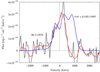 |
Fig. 22. Same as in Fig. 18, but for He Iλ5876 (black, and smoothed in red) instead of [Ne III] λ3869. The [O IIII] profile was multiplied by a factor of 0.01 to match the He I line. LMC rest frame velocity is marked by a vertical thin line. The red side of the He I line appears depreciated compared to [O IIII], similar to Hβ in Fig. 15. |
Through slit 2 we also detect [Ar III] λ7136 and [Ni II] λ7378 with intensities relative to [O III] λ5007 similar to what was reported by Kirshner et al. (1989) (cf. Table 2). On the other hand, the modeled [Ar III] λ7136 flux by Williams et al. (2008) was more than twice as high as the observed relative flux of the line. This could suggest that Ar/O is less than the value of 0.1 assumed by Williams et al. (2008). Tuning the model results of Williams et al. (2008) with the observed [Ar III] λ7136 fluxes then suggests MAr/MO ∼ 0.02. The nucleosynthesis yields in the model of Sieverding et al. (2020) give the same value, that is, MAr/MO ∼ 0.02 for the total yield of Ar and O. The ratios in Chieffi & Limongi (2013) are ∼0.01 for 13 − 20 M⊙ rotating, and 20 M⊙ for nonrotating progenitors, whereas the ratio is higher, ∼0.02, for 13 M⊙ nonrotating progenitors. Our multilevel model atoms suggest MAr/MO = 0.015(0.030) for equal ionization zones of Ar2+ and O2+ in the SNRC and for temperatures of 20 000 (30 000) K. The observed level of [Ar III] λ7136 is therefore consistent with that expected from elemental yields in progenitor models, and with [O III] temperatures.
As shown in Fig. 17 ([Fe III] λ4986), Fig. 20 ([Fe V] λ3726), and Fig. 23 ([Fe II] λ5159, [Fe III] λ5270, [Fe V] λ4227 and [Fe VII] λ5721), we detect several forbidden iron lines through slit 1, with decent signal-to-noise. We also detect [Fe II] λλ4287,4414,5044, [Fe III] λ4658,4881,4986, [Fe V] λλ3783−3797, and [Fe VII] λ5721. The strongest line is [Fe III] λ4658, but it blends with several other [Fe III] lines, as do also several [Fe II] lines around ∼ 4474 Å. Through slit 2 we detect [Fe II] λ5159 and [Fe III] λλ4658,5270, but with poor signal-to-noise.
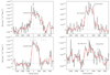 |
Fig. 23. Same as in Fig. 22, but for several forbidden iron lines (black, and smoothed in red) instead of He Iλ5876. The velocities are centered on LMC rest frame velocities of [Fe II] λ5159 (upper left panel), [Fe III] λ5270 (lower left), [Fe V] λ4227 (upper right), and [Fe VII] λ721 (lower right). In each panel gray arrows mark velocities for other nebular lines seen in SNRs (Fesen & Hurford 1996). In particular, [Fe II] λ5159 could be blended with (and even dominated by) [Fe VII] λ5159. We note broad wings of [Fe V] λ4227, possibly reaching ± 2000 km s−1. |
We have chosen to concentrate on presumably unblended lines observed through slit 1. In general, the line profiles are similar to those of the [O II] lines. In particular this is the case for [Fe III] λ5270 and the core of [Fe V] λ4227, whereas [Fe VII] λ5721 is noisy, and perhaps also affected by [N II] λ5755 in the far red wing. In Fig. 23 we have marked the velocities corresponding to other lines detected in SNRs (Fesen & Hurford 1996), which could perhaps contribute to the lines we have highlighted. For example, [Fe II] λ4247 could contribute to the red wing of [Fe V] λ4227, and our identification of [Fe II] λ5159 could instead be dominated by [Fe VII] λ5159, in particular since we also detect [Fe VII] λ5721. To test this we have used our nine-level model atom for Fe6+, including data from Berrington et al. (2000) and Del Zanna et al. (2021, and references therein). For ne = 103 cm−3 and T = 30 000 K, the expected strongest [Fe VII] lines are (in order and normalized to [Fe VII] λ5721): [Fe VII] λ6089, [Fe VII] λ3759, [Fe VII] λ3587, [Fe VII] λ4990, and [Fe VII] λ5159 with relative strengths 1.9, 1.4, 1.0, 0.7, and 0.5, respectively. Unfortunately, [Fe VII] λ3587 and [Fe VII] λ6089 are outside the spectral range of our slit 1 observations, although the latter line can, after smoothing, be hinted in the NTT/EMMI spectrum. [Fe VII] λ3759 is clearly detected through slit 1, and [Fe VII] λ4990 may add to [Fe III] λ4986 in Fig. 17. Judging from the weak measured flux of [Fe VII] λ5721, and that [Fe VII] λ5159 is not expected to be stronger, we conclude that the spectral line at ∼5171 Å (and ∼5160 Å through slit 2) is dominated by [Fe II] λ5159. The line has a possible broad blue wing, which is also hinted for [Fe V] λ4227 (cf. Fig. 23). However, since no such wing is expected for [Fe II] lines, it is probably not real. Deeper observations are needed to check the wing of the [Fe V] line.
3.4.2. Masses and abundances – a summary
In the previous section we estimated the relative abundances in 0540. We now summarize this and estimate the total ejecta mass of the elements we have discussed. The mass of O2+ ions in the SNRC emitting [O III] λ5007 is
![Mathematical equation: $$ \begin{aligned}&M(\mathrm{O}^{2+}) \approx 3.2\times 10^{-5}\ \left( \frac{f_{[{\text{O}}{\small{\text {{ III}}}}]\lambda 5007}}{10^{-13}\ \mathrm{erg\ cm}^{-2}\ \mathrm{s}^{-1}} \right) \left( \frac{D}{50\ \mathrm{kpc}} \right)^{2} \nonumber \\&\qquad \quad \left( \frac{n_{\rm e}}{10^{3}\ \mathrm{\,cm}^{-3}} \right)^{-1} \left( \frac{j_{[{\text{O}}{\small{\text{ III}}}]\lambda 5007}}{10^{-21}\ \mathrm{erg\ cm}^{3}\ \mathrm{s}^{-1}\ \mathrm{sr}^{-1}} \right)^{-1} \ \,{M}_\odot . \end{aligned} $$](/articles/aa/full_html/2022/02/aa41931-21/aa41931-21-eq17.gif) (3)
(3)
Here f[O III]λ5007 is the dereddened flux for one of the slit positions with a slit correction included to account for the full SNRC. For the SNRC we get f[O III]λ5007 ∼ 3.0 × 10⁻¹³ erg cm−2 s−1. j[O III]λ5007 is the emissivity of the λ5007 transition, which for T = 23 500 K is ∼1.1 × 10⁻²¹ erg cm3 s−1 sr−1. For ne = 103 cm−3 one then gets M(O2+)∼9 × 10⁻⁵ M⊙.
A similar estimate for M(O+) from [O II] λλ3726,3729 gives M(O+)∼5 × 10⁻⁵ M⊙ when we use T = 20 000 K (and from this j[O III]λλ3726,3729 ∼ 1.1 × 10⁻²¹ erg cm3 s−1 sr−1). A combined mass of M(O+)+M(O2+)∼1.4 × 10⁻⁴ M⊙ may seem like a surprisingly low mass considering that about two solar masses of oxygen should be present in 0540 (if similar to, e.g., SN 1987A). However, this estimate is only for the amount of oxygen in the SNRC that has been recently shocked. Those shocks are thin due to intense radiative cooling. The cooling time, calculated from a simple six-level model atom of pure O2+ at T = 30 000 K with ne = 103 cm−3, is ∼0.02 years, and at T = 50 000 K it is ∼0.024 years. The similar numbers for pure O+ at T = 20 000 K and T = 30 000 K are ∼0.023 years and ∼0.02 years. The real cooling time is longer if the shocked gas starts out hotter than T = 50 000 K, although this is not so important since the cooling function for pure oxygen peaks around ∼2 × 10⁵ K (cf. Borkowski & Shull 1990), and falls monotonically toward lower temperatures. More important is that the cooling is counteracted by photoionization of ambients photons from the PWN. With this in mind, a lower limit on the cooling time is ∼0.05 years. Thus, ∼1.4 × 10⁻⁴ M⊙ has to be replenished every ≳0.05 years, which means ∼0.3 M⊙ of shocked oxygen in ≳100 years.
Williams et al. (2008) did shock modeling for a similar situation where they assumed a low-velocity shock of 20 km s−1 aided by photoionization of PWN photons to account for the heavy-element ejecta lines. This is much lower than the shock velocity in Borkowski & Shull (1990) for Cas A, although that study only included preionization by photons produced by the shock. The oxygen column density of the emitting region in Williams et al. (2008) is ∼1014 cm−2, and the mass flux of ejecta flowing into the low-velocity shocks is ∼0.01 M⊙ yr−1, which appears consistent with our estimate of ≲0.003 Xother M⊙ yr−1, where Xother > 1 is the correction factor to include all elements, and not only oxygen.
The mass fractions we estimated in Sect. 3.4.1 for the SNRC of 0540, namely O : Ne : S : Ar = 1 : 0.07 : 0.10 : 0.02 and H : He = 1 : ≳0.8, are thus sampled over a very small fraction of the inner ejecta at any given time. How representative these numbers are for all inner ejecta is not very clear. However, one could imagine that there could be fluctuations on moderate time scales if the low-velocity shocks run into regions which are not fully microscopically mixed. This could be the reason for the apparent elevated sulfur abundance indicated by our NTT/EMMI observations.
We highlight that fluctuations in line ratios may also be caused by magnetic fields. As discussed by Hartigan et al. (1994) and Hartigan & Wright (2015), a strong field in the cooling region lowers the density of the shocked plasma (due to the added magnetic pressure), which extends both the cooling times and the size of the cooling zone. For metal-rich plasmas with very rapid cooling times, such as discussed here for 0540, and discussed by Blair et al. (2000) for SNRs N132D and 1E0102-7219, one could imagine time-varying cooling and relative line fluxes depending on changes in the post-shock magnetic field strength. In this case, line intensity ratios for lines of even the same ion could fluctuate. For the oxygen-rich ejecta of 0540, one such ratio is I[O II] λλ3726,3729/I[O II] λλ7319−7331 which is density sensitive. For a temperature of 20 000 K, our multilevel model atom shows that this intensity ratio is ≳20, ∼12 and ∼7 for the electron densities 102 cm−3, 103 cm−3, and 3 × 103 cm−3, respectively. that is, for the range of electron densities discussed by Sandin et al. (2013). A weak magnetic field would thus limit the flux of [O II] λλ3726, 3729 due to larger compression and, as a consequence, collisional deexcitation, while [O II] λλ7319 − 7331 would be less affected.
3.4.3. The halo and beyond
Added to the mass of the SNRC is the mass of ejecta in the unshocked freely moving supernova ejecta. According to Williams et al. (2008), the inner part of this is photoionized to O2+, so we use Equation 3 with ne = 1 cm−3 and f[O III]λ5007 ∼ 1.5 × 10⁻¹³ erg cm−2 s−1, which corresponds to the integrated broad base of [O III] emission in Fig. 19, and assuming that the VIMOS/IFU field-of-view misses roughly one third of the halo emission. For the photoionized halo we further assume a temperature of ∼12 000 K, so that j[O III]λ5007 ∼ 4 × 10⁻²² erg cm3 s−1 srs−1. With these assumptions, the mass of O2+ in the halo, M(O2+)halo ∼ 0.12 M⊙. The mass is most likely higher since ne = 1 cm−3 only stems from the 4 a.m.u. at the inner boundary of the unshocked SN ejecta estimated by Williams et al. (2008). The average electron density could be ne < 1 cm−3 in the unshocked [O III] emitting halo. According to Williams et al. (2008), enough ionizing photons are produced to ionize ∼1 M⊙ halo ejecta. In a mixed abundance model by Blinnikov et al. (2000) for SN 1987A, which contains ∼2.0 M⊙ of oxygen, with a drop in mass fraction just short of 2000 km s−1, the mass fraction of oxygen falls from ∼0.3 from ∼ 1300 km s−1 to well below 0.1 at 2000 km s−1. Choosing 0.1 for the 0540 halo makes our estimate for M(O2+)halo consistent with the ionized mass estimated by Williams et al. (2008), and if the total oxygen mass is similar to that in SN 1987A, roughly half of the oxygen is now confined to the filaments in the SNRC.
In SN 1987A, the total mass inside 2000 km s−1 is dominated by He, O, and H (cf. Blinnikov et al. 2000). We may assume the same situation for 0540. For a density of 4 a.m.u. at the inner boundary of the halo, corresponding to Vhalo,inner ∼ 1200 km s−1, and an outer velocity for the ionized halo of Vhalo,outer ≳ 1900 km s−1 (as is indicated by our results here), the total mass in this shell is ∼6.8 M⊙, assuming a flat density profile of the unshocked ejecta (cf. Williams et al. 2008). This compares well with the mixed model for SN 1987A by Blinnikov et al. (2000) in which the total mass inside the radius corresponding to this velocity is about 5 − 6 M⊙. It therefore seems that 0540 and SN 1987A could be fairly similar, and perhaps stem from progenitors with roughly similar zero-age-main sequence masses. The main difference between the dynamics in these events is of course the influence of a pulsar, which, if existent in SN 1987A (e.g., Cigan et al. 2019; Greco et al. 2021; Alp et al. 2021), plays a much smaller role than in 0540. On top of that, one has the 3D effects stemming from the explosion hydrodynamics, and possibly pre-explosion rotation. In our mass estimates for the halo we have compared with models assuming 1D, but from Sect. 3.2 it is evident that the halo is far from spherically symmetric. This obviously introduces uncertainties in our mass estimates for the halo.
Moving further away from the SNRC, we introduced in Sect. 3.3.2 five interesting filaments which we have named F1–F5. For all filaments, the spectral lines are unresolved, except for F1, which displays broad bases of the [O III] λλ4959,5007 line profiles, skewed to the red as compared to the positions of the narrow and strong (unresolved) peaks of these lines (cf. Fig. 24). The minimum and maximum velocities of the base (relative to LMC) are at least − 900 km s−1 and + 1300 km s−1, with a possible extension in the red to even larger velocities. No such features are seen in spectra of F2-F5. The presence of the broad base is consistent with the fact that F1 is projected onto the region showing the faint [O III] glow (cf. Fig. 10, top panel). As seen in the lower panel of Fig. 10, high redshifted velocities from the glow (which is emitted by the halo discussed above) occur close to the position of F1. Despite its projected proximity to the SNRC, the unresolved spectral components of filament F1 are therefore not part of the inner region of the SNR itself (see also below).
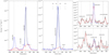 |
Fig. 24. Spectra of forbidden lines from F1 (cf. Figs. 5 and 13). All spectra are in the LMC rest frame, and the velocities are for [O III] λ5007 (left), 3727.5 Å (middle), [Fe II] λ5159 (upper right), and [Fe XIV] λ5303 (lower right). For the oxygen lines, the line profiles of the emission from the SNRC in Figs. 16 and 20, multiplied by a factor of 0.01, have been included for comparison (in red). The narrow spectral lines are unresolved, as highlighted for [O III] λ5007 and the [O II] doublet, where the solid black lines show Gaussians with the expected FWHM of the instrument at 5007 Å and 3727.5 Å, i.e., ∼ 355 km s−1 and ∼ 476 km s−1, respectively. Note the broad bases seen for [O III] and possible broad base wings for [O II] λλ3726,3729. Lines of the H I Balmer series are marked in the middle panel. For the iron lines, Gaussians have also been drawn (in blue) according to the expected resolution. Several other lines have also been indicated. Red marks Savitzky-Golay fitting to the spectrum. |
In Sect. 3.2 we connected the maximum recession velocity of the glow at F1 to the pulsar age. For a maximum velocity of ≳ + 1200 km s−1, the pulsar would be older than 1200 years. Figure 24 shows that this could be the case. However, a maximum velocity of + 1300 km s−1 at the position of F1 would imply vtrue ∼ 2130 km s−1 for a pulsar age of 1200 years, which in turn would correspond to a radius of  , rather than
  in Fig. 5 for the same expansion as vtrue in the westward direction orthogonal to the line-of sight. Figure 5 does not really support this, which could indicate aspherical symmetry of the fastest glow even on smaller scales. Unfortunately, the VIMOS/IFU field does not reach this far from the pulsar to test the degree of nonsphericity over a larger scale, but Fig. 19 shows that even within the 13″ × 13″ field of view of VIMOS, there is large asymmetry of the fast “glow”. However, at the position of F1 specifically, the broad base is fairly symmetric, and less redshifted than the emission from the SNRC (highlighted in red in Fig. 24). Given the results in Sect. 3.2 and what is shown in Fig. 24, the pulsar age is closer to 1200 years than 1100 years.
Figure 24 also shows the [O II] λλ3726,3729 doublet along with [Fe II] λ5159, [Fe XIV] λ5303, and other lines as marked in Fig. 24. [Fe II] λ5159 and [Fe III] λ5270 both showed hints of broad wings for the SNRC. Nothing like that is seen for the position at F1, but this could be due to the limited signal-to-noise. Of greater importance are the two spectral bumps on each side of the central unresolved blend of the [O II] doublet. One possible interpretation is that they originate in the same part of the ejecta as the [O III] halo, and possibly in its outermost part as a result of a transition of the photoionized state from O2+ to O+, at vtrue ∼ 2000 km s−1. Another possibility is that the bumps are due to Balmer lines emission from F1. We have marked the positions of them in the middle panel of Fig. 24. On the blue side, H Iλλ3712,3722 emit at ≈ − 1 249 km s−1 and ≈ − 443 km s−1, respectively (when we center on 3727.5 Å), but on the red side, no H I line fits. Moreover, the strengths of the λ3712 and λ3722 lines are expected to be < 1% of [O II] λλ3726,3729, using Hβ as template. Deeper observations are needed to test the [O II] interpretation, along with photoionization modeling like that in Williams et al. (2008).
Closing in on the narrow components of the lines from the filaments, the weighted velocity of individual lines can be used to test both the physical velocity of the filaments and to check possible systematics in the wavelength calibration. The calibration is problematic far in the very blue due to warped spectra, which makes the velocities for [O II] λλ3726,3729 systematically low. As an example, we show in Fig. 25 the velocities of the detected lines across the spectrum for F1. The velocity of [O II] λλ3726,3729 was estimated using 3727.5 Å (see below). We note that a group of lines tend to have LMC redshift, while most lines cluster at ∼ + 120 km s−1 compared to the LMC. The dashed lines in Fig. 25 show 1σ uncertainties for the wavelength solution. Taking the extremes of this fit (i.e., the solid line in the figure) to assign a combined uncertainty, we arrive at 355 ± 30 km s−1 for F1. For the other filaments we find 260 ± 25 km s−1 for F2, 290 ± 30 km s−1 for F3, 255 ± 20 km s−1 for F4, and 240 ± 20 km s−1 for F5. This means that all of them have velocities consistent with LMC velocity, except for F1, which is redshifted by an extra 85 ± 30 km s−1.
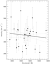 |
Fig. 25. Velocities estimated for emission lines from Filament F1. No doublets or multiplets are included except [O II] λλ3726,3729. As can be seen, the wavelength calibration is stable across the spectrum. Interestingly, there is a group of lines with LMC redshift, although the majority has a redshift close to ∼ + 120 km s−1 compared to LMC redshift. See Table 3 and text for further details. |
In Table 5 we list [O III] temperatures of all filaments. The temperatures were calculated in the same way as for the SNRC in Sect. 3.3.2. For the filaments, we have assumed an electron density of ne = 103 cm−3 (see below), but the difference in estimated temperature is very small for electron densities in the range 102 − few × 103 cm−3. The temperature is highest for F1. If we include [O III] λλ4959,5007 with its full base, we get (3.6 ± 0.4)×104 K. However, from the Gaussian fit for [O III] λ5007 in Fig. 25 we estimate that only ∼60% of the flux is in the spectrally unresolved component. If the base originates in a photoionized halo with a presumed temperature of ≲2 × 10⁴ K, no base is expected to be detected from F1 for the weak [O III] λ4363 line, which is also confirmed by our data. For the unresolved component, a better estimate of the [O III] temperature could therefore be ≳5.5 × 10⁴ K. For the other filaments we estimate (3.0 ± 0.4)×104 K (F2), (1.8 ± 0.2)×104 K (F3) (1.9 ± 0.2)×104 K (F4), and (2.5 ± 0.4)×104 K (F5). The temperatures are somewhat higher than reported in our preliminary analysis in Serafimovich et al. (2005). For the central peak of [O II] λλ3726,3729, we tested possible skewness to reveal the density of F1 (cf. Sect.3.4.1 for how I[O II] λ3729/I[O II] λ3726 depends on density). Unfortunately, the spectral resolution is too poor to draw any such conclusions.
The spectra of all filaments show many forbidden iron lines. Filaments F1 and F3 have lines of [Fe II] and [Fe III], whereas F2 also shows [Fe V] λ4227. Filaments F1, F4, and F5 show the very highly ionized [Fe XIV] λ5303 (cf. Fig. 24), possibly with some contamination from [Ca V] λ5309. There is also a line at λ5537.9 for F1 that could be [Ar X] λ5534. Based on these findings, the X-ray morphology of the remnant, the filament dispositions (cf. Fig. 2), and the high temperatures of the filaments, it is likely that filaments F1, F2, F4 and F5 are ionized by the SNR, most likely through shock activity. Filament F3 sits 1 4 east of the pulsar and has no physical connection to the remnant. However, it is not a normal H II region in the LMC. Typical [O III] temperatures in, for example, the 30 Doradus region vary rather mildly (±140 K) from the average value of 10 270 K (Krabbe & Copetti 2002). The high [O III] temperature of F3, 18 000 ± 2000 K, suggests that it too is affected by the remnant, presumably through intense photoionization by high-energy photons.
Brantseg et al. (2014) studied the radio and X-ray emission from 0540, and we note that one of the regions they studied in detail includes our filament F4. Their models of the detected X-ray emission from this region indicate a shock temperature of Ts ∼ 7 × 10⁶ K. Three of the five other outer SNR regions they studied have similar temperatures, whereas the two other are cooler and hotter by a factor of ∼2. Using the Rankine-Hugoniot relations for fully ionized plasma, this translates into a shock speed of Vs ∼ 510 km s−1 for the region including F4 (e.g., Brantseg et al. 2014). Brantseg et al. (2014) argue for a sufficiently short timescale for temperature equilibration between electrons and ions, and we we use this here as well. Brantseg et al. (2014) also estimated the electron density of the X-ray-emitting regions, and arrive at ne ∼ a few cm−3, and for the region including F4 in particular,  .
.
A shock with velocity Vs ∼ 510 km s−1 can collisionally ionize iron up to Fe18+, with almost no iron in Fe13+ if the plasma is in collisional equilibrium (e.g., Arnaud & Raymond 1992). However, with the low densities in the shocks studied by Brantseg et al. (2014), collisional equilibrium is not fully established, and one has instead to resort to nonequilibrium ionization. More specifically, the collisional ionization time-scale of Fe13+ to Fe14+ is
 (4)
(4)
where Cion(Fe13+) is the collisional ionization rate coefficient for collisions from Fe13+. We use the formalism of Arnaud & Rothenflug (1985) which gives Cion(Fe13+) ≈ 6.8 × 10⁻¹⁰ cm3 s−1 for Ts ∼ 7 × 10⁶ K, which means tion(Fe13+) ∼ 12 years for ne = 4.0 cm−3. The corresponding time scales tion(Fe14+), tion(Fe15+) and tion(Fe16+) are ∼15 years, ∼29 years and ∼230 years, respectively. For young enough shocks, there will certainly be no iron ionized beyond Fe16+, and for shocks younger than a couple of decades, Fe13+ should still be present. Brantseg et al. (2014) estimated an ionization time scale of ∼1600 years for ne = 4.0 cm−3, which seems unreasonably long for F4, unless the density of the shocked gas is substantially higher than 4.0 cm−3. This could be the case for a low filling factor of the shocked gas.
The ionization time scales should be compared with recombination time scales, and for the recombination from Fe13+ to Fe12+, trec(Fe13+), we write
 (5)
(5)
where αrec(Fe13+) is the recombination rate coefficient. If we use the results of Schmidt et al. (2006), that is, αrec(Fe13+) ≈ 1.55 × 10⁻¹¹ cm3 s−1 at Ts ∼ 7 × 10⁶ K, we get trec(Fe13+) ∼ 510 years for ne = 4.0 cm−3. This means that once ionized to Fe13+, the ISM shocked by SNR 0540-69.3 would not have time to recombine. Collisional ionization to Fe14+ is far superior, which immediately shows that the low-density shocked ISM with ne = 4.0 cm−3 is not the source of the low-ionization lines from filament F4.
This is further strengthened if we study the cooling time of the shocked gas. For this we use an expression for the shocked circumstellar matter of SN 1987A, which reads (Gröningsson et al. 2006), valid for 100 km s−1 ≲ Vs ≲ 600 km s−1,
 (6)
(6)
Here nfilament is the density of the filament. Even though this expression was tailored for the enriched He and N abundances of SN 1987A, it is obvious that the cooling time for 0540 is far too long for the shocked gas to cool down to the temperature derived from [O III].
From our discussion, we find that the shocks running into the low-density ISM are adiabatic. Fe13+ is most likely in a transitory state to becoming further ionized, although full collisional equilibrium will not be attained. This plasma cannot be the same as that emitting low-ionization like, for example, [O III] (see below). The situation could therefore be similar to that in the Cygnus Loop (Ballet et al. 1989; Fesen & Hurford 1996; Raymond et al. 2015), N49, N63A, N103b, N132D, and SN 1987A in the LMC (Danziger & Dennefeld 1976; Murdin et al. 1978; Dopita & Mathewson 1979; Blair et al. 2000; Gröningsson et al. 2006; Dopita et al. 2019), Puppis A (Clark et al. 1979), and SNR S8 in IC 1613 (Fesen & Weil 2020), all in which coronal iron lines coexist with lower-ionization iron lines. The situation is different from that in, for example, SNR 1E0102.2-7219 in the SMC (Vogt et al. 2017), where only coronal lines are seen, nicely tracing the blast wave. We return to [Fe XIV] λ5303 below.
The low-ionization lines from F1, F2, F4, and F5 likely originate as results of shocks with lower velocity than the shocks studied by Brantseg et al. (2014). From Filament F1 we detect Fe6+ lines, and in collisional equilibrium this ion peaks in abundance at ∼(2 − 3)×105 K, corresponding to a shock speed of ∼ 100 km s−1. Since we expect the shock speed in the filaments to scale as  , the density of the filaments emitting the low-ionization lines should be ∼ 4.0(VX−ray/Vopt)2 cm−3, where VX − ray and Vopt are the shock speeds in the X-ray emitting region and low-ionization line emitting region, respectively. This points to nfilament ∼ 102 cm−3 for the low-ionization line emitting regions. According to Equation 5, this would mean tcool ∼ 13 years (for Vopt = 100 km s−1). These shocks are therefore radiative (as opposed to the adiabatic shock created by the blast wave). If the postshock gas is in near pressure equilibrium, the density in the [O III]-emitting region should be a factor of ∼10 higher than that emitting [Fe VII] lines, that is, ∼ 103 cm−3. This justifies our choice of 103 cm−3 when we estimated the [O III] temperature earlier in this subsection. A decisive measurement for this picture would be to measure the density from [O II] and/or [S II]. Unfortunately, [S II] emits outside the spectral range of our filament spectra, and the spectral resolution is too low to draw conclusions from [O II].
While four of our filaments have velocities consistent with LMC velocity, Figs. 24 and 25 show that filament F1 recedes by 85 ± 30 km s−1 compared to the others. This is also the only filament which is not situated at, or outside the projected position of the blast wave. According to the Rankine-Hugoniot shock relations for polytropic index γ = 5/3, this means that the shocked gas in the low-ionixzation line-emitting medium is accelerated to 3Vopt/4. For a spherically- symmetric model with a shock radius corresponding to ∼20″ − 25″ at the distance of LMC, and  for the projected distance between the pulsar and F1, the observed 85 ± 30 km s−1 for F1 translates into 90 ± 35 km s−1. If we correct for the factor 4/3, we arrive at Vopt = 120 ± 45 km s−1, which is fully consistent with what we estimated from the estimated shock velocity required to ionize up to Fe6+ for a radiative shock being responsible for the low-ionization lines. In reality, there are most likely a range of shock velocities depending on the distribution of densities, much in the same way as for the well-studied inner ring of SN 1987A (Gröningsson et al. 2006). We reiterate that the broad and narrow lines from the F1 region come from completely different components; the broad [O III] lines come from the halo of freely coasting SN ejecta, while the narrow lines come from the shocks at the SNR front on the rear side of the remnant. Filaments F2, F4, and F5 are moving mainly orthogonal to the line-of-sight, and do not show any blue- or redshift compared to LMC velocity.
In this picture, the [Fe XIV] λ5303 velocity for F1 should be more redshifted than lines from low-ionization ions, that is, if it comes from behind the blast wave. Although [Fe XIV] λ5303 may be slightly more redshifted than the bulk of the emission lines (cf. Table 3 and Fig. 25), we do not see a several hundred km s−1 difference in velocity. There could be at least two explanations for this. The first is that we have misinterpreted another spectral line for being [Fe XIV] λ5303, and the second is that if [Fe XIV] λ5303 is indeed the correct identification, it is not emitted immediately behind the inter-cloud fast shock. Instead it originates from closer to the clouds. To check the first explanation, we focus on the right panels of Fig. 24 in which the stronger iron lines peak around 130 − 140 km s−1, whereas [Fe XIV] λ5303 peaks at ∼ 180 km s−1. The Gaussian fit to [Fe XIV] λ5303 is consistent with a single feature. The FWHM is ≈ 335 km s−1, so any thermal broadening of the line is impossible to trace. That the line may appear somewhat broader than the Gaussian fit is likely due to poor signal-to-noise. In the line list by Fesen & Hurford (1996), there are a few lines close to [Fe XIV] λ5303, namely [Fe II] λ5297 and [Ca V] λ5309. (None of them are marked in Fig. 24). Their velocities relative to [Fe XIV] λ5303 are − 340 km s−1 and + 357 km s−1, respectively. Whereas there is no hint for the [Fe II] line, [Ca V] line could be responsible for a possible slight extension of the [Fe XIV] λ5303 main part of the line feature. This is why we have added the [Ca V] λ5309 line in Tables 3 and 4. That [Fe XIV] λ5303 is present seems solid.
A model for the narrow lines from F1 must explain why [Fe XIV] λ5303 is not more redshifted than the lower-ionization iron lines in Fig. 24. The results of Miceli et al. (2006) may provide a clue. These authors performed 2D axial symmetric simulations of a fast shock interacting with a cloud in a tenuous medium. The setup was intended to model the X-ray emission from the Vela SNR, but general conclusions can be drawn. They tested two geometries, a spherical cloud, and an elliptical cloud with major axis along the shock direction (to simulate a filament). In the spherical cloud case (which we concentrate on), the shock interaction results in something like a two-temperature situation, where soft X-rays are produced in the transmitted shock in the cloud, and a higher-temperature region in the shocked tenuous medium emits harder X-rays. What is important is that the hard X-ray emission does not mainly come from region immediately behind the blast wave. It instead comes from a halo around the cloud. Conduction between the cloud and the hot shocked tenuous medium drives an evaporation of the cloud and the formation of a hot diffuse halo. We suggest that [Fe XIV] λ5303 originates in this zone along with the hard X-rays. As this zone is tied to the cloud, there should not be any significant difference in velocity as determined from the line profiles. Future tests of this scenario would be to study the 0540 filaments in higher spectral resolution, as well as in the red part of the spectrum to probe, for example, [Fe X] λ6374 and [Fe XI] λ7892, as well as to measure the [S II] density.
We note that Blair et al. (2000) discussed a similar situation for their knot P1 in N132D, interpreted as a dense (∼ 200 cm−3) ISM cloudlet being hit by the SNR blast wave, as we do for the 0540 filaments. They concluded, after thorough shock modeling, that the cloudlet N132D−P1 is hit by shocks with a range of velocities between 40 km s−1 and 240 km s−1, and that those shocks are radiative, compressing the shocked gas to densities well above 103 cm−3. The ram pressure of those shocks are of the same order as that of the main blast wave shocking interstellar gas at another position of the remnant where the ISM density is estimated to be ∼ 3 cm−3 (Morse et al. 1995). Blair et al. (2000) detected [Fe XIV] λ5303 in N132D−P1, just as we do for F1, F3, and F4 in 0540, but [Fe XIV] λ5303 was not included in the models of Blair et al. (2000). It seems reasonable that the [Fe XIV] λ5303 emission in N132D−P1 could be explained in a similar fashion as we suggest for the 0540 filaments, especially since the blast wave propagates at ∼ 800 km s−1 in N132D at the position studied by Morse et al. (1995) and referred to here, that is, even faster than for the F4 region of 0540.
Moving to regions in the southwestern part of SNR 0540-69.3, the possibly N-rich filament identified by Mathewson et al. (1980) is outside the reach of our slits, and the field-of-view of the VIMOS/IFU of Sandin et al. (2013). However, our NTT/EMMI slit covers a region close to it which shows strong nebular emission. In Fig. 26, we show this region and its spectrum, dereddened using EB − V = 0.19, and normalized to [O III] λ5007. (The region discussed by Mathewson et al. 1980, is marked with an “M”.) The electron density from [S II] in the yellow-marked region along the EMMI slit is ≲ 102 cm−3, which is fully consistent with an H II region in the LMC, as is also the velocity of the emitting region. However, there is an oddity with the overall spectrum in that it is very red. With EB − V = 0.19 the Balmer decrement Hα/Hβ ∼ 5.0., which is almost a factor of ≈1.8 higher than expected from an H II region. The simplest solution to this is that the emission comes from an H II region, but that EB − V ∼ 0.95 for this area, rather than the value we use for 0540. From a visual inspection of Fig. 1, it is clear that the nebulous emission is less pronounced in an area that includes both the yellow part along the slit in Fig. 26 and the region M highlighted by Mathewson et al. (1980). Absence of [O III]-emission is also very clearly seen for this region in Fig. 1A of Mathewson et al. (1980). Such a patchy structure is expected if there are dusty regions embedded in a large H II region like N 158 (Henize 1956) with its superbubble around the OB association LH 104 in the north (Lucke & Hodge 1970; Testor & Niemela 1998). which dominates this part of the LMC. Finally, we note that the filter used by Mathewson et al. (1980) to study [N II] was centered on 6584 Å with a FWHM of 16 Å. With an LMC redshift of 270 km s−1, Hα is redshifted to ∼6569 Å and [N II] λ6584 to 6589 Å. In the spectrum of Fig. 26, I[N II]λ6584/IHα ∼ 2.2, and if this is also the case for region “M”, ∼20% of the emission in the 6584 Å filter used by Mathewson et al. (1980) is due to Hα (if Gaussian), however, the exact fraction being sensitive to the transparency of the blue wing of their 6584 Å filter.
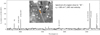 |
Fig. 26. Spectrum of a region (marked in yellow) along the NTT/EMMI slit close to the “N-rich” region identified by Mathewson et al. (1980), here marked with “M”. The map in the inset is from Fig. 2. The spectrum was dereddened with E(B − V) = 0.19, and plotted relative to [O III] λ5007. The electron density is from [S II] λλ6716,6731, and the velocity of the emitting gas is LMC rest velocity. See text for further details. |
4. Conclusions
A combination of [O III] filters centered on 0 km s−1 and + 3000 km s−1 was used to reveal structures of filaments in the central part of SNR 0540-69.3 (SNRC), not previously detected by HST filters, and disproves some structures indicated by the VLT/VIMOS integral-field-unit (IFU) observations by Sandin et al. (2013). We detect [O III] emission out to ∼10″ from the pulsar, which corresponds to an average ejecta velocity of ∼ 2000 km s−1 for an age of 1200 years. The filter images complement the IFU images in [O III] to suggest ring-like structures around a symmetry axis from northeast to southwest, also seen in [S II] (Sandin et al. 2013). In a 3D-representation, the symmetry axis crosses the projected pulsar position ∼ 500 km s−1 on the receding side of the remnant, which if it is due to pulsar activity, could indicate that the pulsar shares the same general redshift as the SNRC. Such pulsar activity could occur if the pulsar jet is oriented along this axis rather than as displayed in Fig. 6. It is emphasized that there is evidence for substantial past and present activity along the suggested jet axis (cf. Lundqvist et al. 2011), but the rings could also have an origin related to the supernova explosion.
SNR 0540-69.3 was also studied through two slits roughly orthogonal to each other (PA = 22° and PA = 88°). Several new spectral lines are identified for the SNRC, and 2D spectroscopy along the slits reveals fast [O III]-emitting ejecta outside the SNRC corresponding to a space velocity of vtrue ∼ 2100 km s−1 on the receding western part. This velocity agrees with our imaging, as well as a pulsar age of ≈1200 years, which is much less than the spin-down age of the pulsar (≈1600 years, Reynolds 1985). 0540 is therefore the remnant of one of the most recent supernovae in the LMC. While SN 1987A is obviously the youngest, Kirshner et al. (1989) and Morse et al. (2006) discussed that 0540 could be the second youngest. This may still be the case for core-collapse SNe (Maggi et al. 2016), but a few Type Ia SNRs are younger, with the 400 ± 120 year old SNR J0509−6731 likely being the youngest (Rest et al. 2005).
In the southwest, on the receding side, vtrue ≳ + 2200 km s−1. On the approaching side, the [O III] emission reaches vtrue ∼ 1900 km s−1. Although substantially weaker, [Ne III] emission has similar structure to that of [O III], whereas [O II], [S II], [Ar III], and Hβ are emitted by the more compact structure of the SNRC, in agreement with the [S II] IFU image of Sandin et al. (2013). The luminosity-weighted average of the lines is +440 ± 80 km s−1 with respect to the host galaxy, which is in accord with previous findings, as well as the possible pulsar motion.
The average [O III] temperature of filaments in the SNRC is 23 500 ± 1800 K, which is somewhat lower than previously reported, mainly because we have included a correction of the [O III] λ4363 flux due to the blend with Hγ. The electron density derived from [S II] λλ6716,6731 is found to be ne ∼ 103 cm−3, which is slightly higher than in the density map of Sandin et al. (2013).
The VIMOS/IFU data of Sandin et al. (2013) were used to construct slit correction factors for our spectroscopic data in order to estimate overall abundances and masses of various elements for the filaments in the SNRC. Infrared data from Spitzer (Williams et al. 2008) were also included in these estimates. In particular, relative mass ratios were found to be O : Ne : S : Ar ≈ 1 : 0.07 : 0.10 : 0.02. Those ratios are consistent with explosion models of 13 − 20 M⊙ progenitors (e.g., Chieffi & Limongi 2013; Sieverding et al. 2020), as well as SN 1987A (cf. Jerkstrand et al. 2011). The argon abundance is a factor of ∼2 lower than used in the models by Williams et al. (2008) (which was also suggested by those authors as a possibility). The fact that we detect H and He mixed in deep into the central region is a clear sign of explosive mixing, as in SN 1987A. The mass ratio of He/H in the SNRC is estimated to be at least ∼0.8, which is another similarity with SN 1987A.
The mass of [O II] and [O III] emitting oxygen in the SNRC is only ∼1.4 × 10⁻⁴ M⊙, but the cooling time of shocked gas in the SNRC is so short (≳0.05 years) that the mass flux through the low-velocity shocks in the SNRC can be up to ∼0.003 Xother M⊙ yr−1, where Xother is the correction factor to include all elements, not only oxygen. This is on the low side compared with ∼0.01 M⊙ yr−1 estimated by Williams et al. (2008). The rapid cooling of the shocked gas in the SNRC could in principle make it possible to detect fluctuations in the flux of lines other than those from oxygen if the SNRC is not microscopically mixed. We note a possible such fluctuations in [S II]λλ6716,6731 between 1989–2006. This effect could potentially make abundance estimates for the whole SNRC vulnerable for elements other than oxygen in the SNRC, and also for oxygen if magnetic pressure effects are important. IFU images for various spectral lines separated in time by several years could resolve this uncertainty4. In the mid-infrared, observations with MIRI on the James Webb Space Telescope (JWST) would provide a serious upgrade for the 5 − 28 μm range compared to the Spitzer data presented by Williams et al. (2008), both in terms of sensitivity and spatial resolution. Apart from spectral line information, the localization of 50 − 55 K dust (Williams et al. 2008; Lundqvist et al. 2020) may be constrained. NIRSpec on JWST, with its spectral range of 0.7 − 5 μm, would bridge optical and MIRI data. An interesting possibility to study fluctuations in the SNRC is monitoring by the Vera C. Rubin Observatory, although it may be difficult to separate out fluctuations of spectral lines from fluctuations of continuum emission, such as those discussed by Lundqvist et al. (2011), using broadband filters.
The fastest emitting [O III] ejecta (which have components with velocities in excess of 2000 km s−1) come from a freely coasting halo of photoionized supernova ejecta. The mass of the halo is ∼0.12 M⊙, if spherical symmetry is assumed. However, the halo shows clear asymmetry, with no detectable emission on the receding side to the north, and only weak emission on the approaching side to the south. On the approaching side, there appears to be a “wall”-like feature centered slightly to the northwest of the projected pulsar position, and it has velocities more blueward than ∼ − 750 km s−1. We have used the VIMOS/IFU results of Sandin et al. (2013) to constrain that structure. There is a hint of [O II] λλ3726,3729 emission from fast photoionized ejecta (both approaching and receding), which would mark the outer boundary of the photoionized region. Oxygen-rich ejecta out to ∼ 2000 − 2200 km s−1, and a total mass of oxygen of ∼2 M⊙, are yet other similarities with SN 1987A (cf. Jerkstrand et al. 2011, and references therein for properties of SN 1987A). However, for 0540 most of the oxygen is likely to be located in filaments in a pulsar-wind nebula, which for SN 1987A is not the case.
A third slit was placed along the western part of the supernova remnant shock. Two optical filaments, named F4 and F5, are detected for this slit position, and three further filaments (F1, F2, and F3) are identified for the PA = 88° slit. Although having an [O III] temperature of 18 000 ± 2000 K, filament F3 lies too far from SNR 0540-69.3 to be physically connected to it, and is most likely an H II region in the vicinity of the remnant. The other filaments are hotter, and three of them (F2, F4, and F5) show [Fe XIV] λ5303 emission. The hottest (F1), with an [O III] temperature in excess of 55 000 K, is redshifted by 85 ± 30 km s−1 relative to the LMC redshift, and is located only  west of the pulsar. We argue that the redshift was acquired when F1 was shocked by the SNR blast wave. Similar acceleration for F2, F4, and F5 would have occurred orthogonal to the line of sight since they show no red- or blueshift. Filament F4 overlaps with a region studied in X-rays by Brantseg et al. (2014), and including temperatures and densities from the X-ray modeling by these authors, we conclude that most of the optical lines from F1, F2, F4, and F5 come from radiative shocks in ISM clouds, overtaken by the supernova blastwave. The electron density of the [O III] emitting gas is estimated to be ∼ 103 cm−3. Lines from more highly ionized ions, and in particular [Fe XIV] λ5303, are argued to come from an evaporation zone in connection with the radiatively cooled gas. Future observations of these and possible other filaments at higher spectral resolution is needed to test these conclusions. In addition, an increased spectral range, including UV with the Hubble Space Telescope, and the full optical/NIR range with, for example, ESO/VLT/X-shooter is needed to aid reddening corrections, and for comprehensive shock modeling similar to that in Blair et al. (2000) for N132D-P1.
A portion of the NTT slit with PA = 22° was used to probe a region close to a possibly N-rich filament identified by Mathewson et al. (1980). Our spectrum reveals that the emission is highly reddened with a Balmer decrement of Hα/Hβ ∼ 5.0, and that the emitting gas has a low electron density (≲ 102 cm−3). It is most likely emission from an H II region unrelated to the supernova. The severe reddening boosts red lines compared to, for example, [O III] which is weak in this region. The [N II] filter used by Mathewson et al. (1980) could also have been affected by Hα emission. An N-rich supernova filament in this region therefore seems unlikely.
After this work was completed, new data with MUSE and X-shooter on ESO/VLT were presented in Larsson et al. (2021). Those observations, followed by similar observations in the future, may be used to study fluctuations, although the MUSE IFU data (unlike the X-shooter slit data) do not include, for example, [O II] λλ3726, 3729.
Acknowledgments
We thank R. J. Cumming for helping out with the NTT observations and A. Koptsevich for being part of the preparations of the VLT observations. We are also grateful to C. Fransson, J. Larsson, C. Sandin, and J. Sollerman for discussions, and the referee for insightful comments and suggestions. The research of P. L. is sponsored by the Swedish Research Council. Early on in this project, P. L. was a Research Fellow at the Royal Swedish Academy supported by a grant from the Wallenberg Foundation, and N. L. was supported by the Swedish Institute. YuAS is partially supported by the Russian Foundation for Basic Research (RFBR) according the project 19-52-12013. We made use of the Atomic Line List (Van Hoof 2018), and the CHIANTI data base. CHIANTI is a collaborative project involving George Mason University, the University of Michigan (USA), University of Cambridge (UK) and NASA Goddard Space Flight Center (USA). This research has also made use of NASA’s Astrophysics Data System Bibliographic Services.
References
- Alp, D., Larsson, J., & Fransson, C. 2021, ApJ, 916, 76 [NASA ADS] [CrossRef] [Google Scholar]
- Arnaud, M., & Raymond, J. 1992, ApJ, 398, 394 [CrossRef] [Google Scholar]
- Arnaud, M., & Rothenflug, R. 1985, A&AS., 60, 425 [NASA ADS] [Google Scholar]
- Avila, G., Gero, R., & Beckers, J. M. 1997, in Optical Telescopes of Today and Tomorrow, SPIE 2871, ed. A. Ardeberg, 1135 [Google Scholar]
- Balick, B., & Heckman, T. 1978, ApJ, 226, L7 [NASA ADS] [CrossRef] [Google Scholar]
- Ballet, J., Caplan, J., Rothenflug, R., Dubreuil, D., & Soutoul, A. 1989, A&A, 211, 217 [Google Scholar]
- Berrington, K. A., Nakazaki, S., & Norrington, P. H. 2000, A&AS, 142, 313 [NASA ADS] [CrossRef] [EDP Sciences] [Google Scholar]
- Blair, W. P., Davidson, K., Fesen, R. A., et al. 1997, ApJS, 109, 473 [NASA ADS] [CrossRef] [Google Scholar]
- Blair, W. P., Morse, J. A., Raymond, J. C., et al. 2000, ApJ, 537, 667 [NASA ADS] [CrossRef] [Google Scholar]
- Blinnikov, S., Lundqvist, P., Bartunov, O., Nomoto, K., & Iwamoto, K. 2000, ApJ, 532, 1132 [NASA ADS] [CrossRef] [Google Scholar]
- Borkowski, K. J., & Shull, J. M. 1990, ApJ, 348, 169 [NASA ADS] [CrossRef] [Google Scholar]
- Brantseg, T., McEntaffer, R. L., Bozzetto, L. M., Filipovic, M., & Grieves, N. 2014, ApJ, 780, 50 [Google Scholar]
- Brocklehurst, M. 1971, MNRAS, 153, 471 [Google Scholar]
- Caraveo, P. A., Bignami, G. F., Mereghetti, S., & Mombelli, M. 1992, ApJ, 395, L103 [NASA ADS] [CrossRef] [Google Scholar]
- Caraveo, P. A., Mignani, R., & Bignami, G. F. 1998, Mem. Soc. Astron. It., 69, 1061 [NASA ADS] [Google Scholar]
- Chanan, G. A., Helfand, D. J., & Reynolds, S. P. 1984, ApJ, 287, L23 [NASA ADS] [CrossRef] [Google Scholar]
- Charlebois, M., Drissen, L., Bernier, A.-P., Grandmont, F., & Binette, L. 2010, AJ, 139, 2083 [NASA ADS] [CrossRef] [Google Scholar]
- Chevalier, R. A. 2006, ArXiv e-prints [arXiv:astro-ph/0607422] [Google Scholar]
- Chieffi, A., & Limongi, M. 2013, ApJ, 764, 21 [Google Scholar]
- Cigan, P., Matsuura, M., Gomez, H. L., et al. 2019, ApJ, 886, 51 [NASA ADS] [CrossRef] [Google Scholar]
- Clark, D. H., Murdin, P., Zarnecki, J. C., & Culhane, J. L. 1979, MNRAS, 188, 11 [Google Scholar]
- Danziger, I. J., & Dennefeld, M. 1976, PASP, 88, 44 [NASA ADS] [CrossRef] [Google Scholar]
- Davidson, K., & Fesen, R. A. 1985, ARA&A, 23, 119 [NASA ADS] [CrossRef] [Google Scholar]
- De Luca, A., Mignani, R. P., Caraveo, P. A., & Bignami, G. F. 2007, ApJ, 667, 77 [Google Scholar]
- Del Zanna, G., Dere, K. P., Young, P. R., & Landi, E. 2021, ApJ, 999, 38 [NASA ADS] [CrossRef] [Google Scholar]
- Dopita, M. A., & Mathewson, D. S. 1979, ApJ, 231, L147 [NASA ADS] [CrossRef] [Google Scholar]
- Dopita, M. A., & Tuohy, I. R. 1984, ApJ, 282, 135 [NASA ADS] [CrossRef] [Google Scholar]
- Dopita, M. A., Seitenzahl, I. R., Sutherland, R. S., et al. 2019, AJ, 157, 50 [Google Scholar]
- Fesen, R. A., & Hurford, A. P. 1996, ApJS, 106, 563 [NASA ADS] [CrossRef] [Google Scholar]
- Fesen, R. A., & Weil, K. E. 2020, ApJ, 902, 19 [NASA ADS] [CrossRef] [Google Scholar]
- Ge, M. Y., Lu, F. J., Yan, L. L., et al. 2019, Nat. Astron., 3, 1122 [NASA ADS] [CrossRef] [Google Scholar]
- Gomez, H. L., Krause, O., Barlow, M. J., et al. 2012, ApJ, 760, 96 [NASA ADS] [CrossRef] [Google Scholar]
- Gotthelf, E. V., & Wang, Q. D. 2000, ApJ, 532, L117 [NASA ADS] [CrossRef] [Google Scholar]
- Greco, E., Miceli, M., Orlando, S., et al. 2021, ApJ, 908, L45 [NASA ADS] [CrossRef] [Google Scholar]
- Gröningsson, P., Fransson, C., Lundqvist, P., et al. 2006, A&A, 456, 581 [NASA ADS] [CrossRef] [EDP Sciences] [Google Scholar]
- Hammer, M., Janka, H-Th., & Müller, E. 2010, ApJ, 714, 1371 [NASA ADS] [CrossRef] [Google Scholar]
- Hamuy, N. J., Suntzeff, N. B., & Heathcote, S. R. 1994, PASP, 106, 566 [NASA ADS] [CrossRef] [Google Scholar]
- Hartigan, P., & Wright, A. 2015, ApJ, 811, 12 [NASA ADS] [CrossRef] [Google Scholar]
- Hartigan, P., Morse, J. A., & Raymond, J. C. 1994, ApJ, 436, 125 [NASA ADS] [CrossRef] [Google Scholar]
- Henize, K. G. 1956, ApJS, 2, 315 [CrossRef] [Google Scholar]
- Hester, J. J. 1998, Rev. Mex. Astron. Astrofis., 7, 90 [NASA ADS] [Google Scholar]
- Hwang, U., Petre, R., Holt, S. S., & Szymkowiak, A. E. 2001, ApJ, 560, 742 [NASA ADS] [CrossRef] [Google Scholar]
- Jerkstrand, A., Fransson, C., & Kozma, C. 2011, A&A, 530, 45 [Google Scholar]
- Kirshner, R. P., Morse, J. A., Winkler, P. F., & Blair, W. P. 1989, ApJ, 342, 260 [NASA ADS] [CrossRef] [Google Scholar]
- Kozma, C., & Fransson, C. 1998, ApJ, 497, 431 [NASA ADS] [CrossRef] [Google Scholar]
- Krabbe, A. C., & Copetti, M. V. F. 2002, A&A, 387, 295 [NASA ADS] [CrossRef] [EDP Sciences] [Google Scholar]
- Larsson, J., Sollerman, J., Lyman, J. D., et al. 2021, ApJ, 922, 265 [CrossRef] [Google Scholar]
- Lucke, P., & Hodge, P. W. 1970, AJ, 75, 171 [NASA ADS] [CrossRef] [Google Scholar]
- Lundqvist, N., Lundqvist, P., Björnsson, C.-I., et al. 2011, MNRAS, 413, 611 [NASA ADS] [CrossRef] [Google Scholar]
- Lundqvist, P., Lundqvist, N., Vlahakis, C., et al. 2020, MNRAS, 496, 1834 [NASA ADS] [CrossRef] [Google Scholar]
- MacAlpine, G. M., Lawrence, S. S., Sears, R. L., et al. 1996, ApJ, 463, 650 [NASA ADS] [CrossRef] [Google Scholar]
- Maggi, P., Haberl, F., Kavanagh, P. J., et al. 2016, A&A, 585, A162 [NASA ADS] [CrossRef] [EDP Sciences] [Google Scholar]
- Manchester, R. N., Staveley-Smith, L., & Kesteven, M. J. 1993a, ApJ, 411, 756 [NASA ADS] [CrossRef] [Google Scholar]
- Manchester, R. N., Mar, D. P., Lyne, A. G., Kaspi, V. M., & Johnston, S. 1993b, ApJ, 403, 29 [Google Scholar]
- Maran, S. P., Sonneborn, G., Pun, C. S. J., et al. 2000, ApJ, 545, 390 [NASA ADS] [CrossRef] [Google Scholar]
- Martin, T., Milisavljevic, D., & Drissen, L. 2021, MNRAS, 502, 186 [NASA ADS] [Google Scholar]
- Mathewson, D. S., Dopita, M. A., Tuohy, I. R., & Ford, V. L. 1980, ApJ, 242, L73 [NASA ADS] [CrossRef] [Google Scholar]
- Mattila, S., Lundqvist, P., Gröningsson, P., et al. 2010, ApJ, 717, 1140 [NASA ADS] [CrossRef] [Google Scholar]
- Miceli, M., Reale, F., Orlando, S., & Bocchino, F. 2006, A&A, 458, 213 [NASA ADS] [CrossRef] [EDP Sciences] [Google Scholar]
- Middleditch, R. N., & Pennypacker, C. R. 1985, Nature, 313, 659 [NASA ADS] [CrossRef] [Google Scholar]
- Mignani, R. P., De, A., Hummel, W., et al. 2012, A&A, 544, 100 [Google Scholar]
- Mignani, R. P., Shearer, A., de Luca, A., et al. 2019, ApJ, 871, 246 [NASA ADS] [CrossRef] [Google Scholar]
- Morse, J. A. 2003, Rev. Mex. Astron. Astrofis. Conf. Ser., 15, 243 [NASA ADS] [Google Scholar]
- Morse, J. A., Winkler, P. F., Kirshner, R. P., et al. 1995, AJ, 109, 2104 [NASA ADS] [CrossRef] [Google Scholar]
- Morse, J. A., Smith, N., Blair, W. P., Kirshner, R. P., et al. 2006, ApJ, 644, 188 [NASA ADS] [CrossRef] [Google Scholar]
- Murdin, P., Clark, D. H., & Culhane, J. L. 1978, MNRAS, 183, 79 [Google Scholar]
- Osterbrock, D. E., & Ferland, G. J. 2006, Astrophysics of Gaseous Nebulae and Active Galactic Nuclei (Sausalito, CA: University Science Books) [Google Scholar]
- Patat, F., Moehler, S., O{’}Brien, K., et al. 2011, A&A, 527, A91 [NASA ADS] [CrossRef] [EDP Sciences] [Google Scholar]
- Pavlov, G. G., Zavlin, V. E., Aschenbach, B., Trümper, J., & Sanwal, D. 2000, ApJ, 531, L53 [NASA ADS] [CrossRef] [Google Scholar]
- Pietrzyński, G., Graczyk, D., Gallenne, A., et al. 2019, Nature, 567, 200 [Google Scholar]
- Raymond, J. C., Edgar, R. J., Ghavamian, P., & Blair, W. P. 2015, ApJ, 438, 1132 [NASA ADS] [Google Scholar]
- Rest, A., Suntzeff, N. B., Olsen, K., et al. 2005, Nature, 384, 1200 [Google Scholar]
- Reynolds, S. P. 1985, ApJ, 291, 152 [CrossRef] [Google Scholar]
- Rudie, G. C., Fesen, R. A., & Yamada, T. 2008, ApJ, 384, 1200 [Google Scholar]
- Sandin, C., Lundqvist, P., Lundqvist, N., et al. 2013, MNRAS, 432, 2854 [NASA ADS] [CrossRef] [Google Scholar]
- Schmidt, E. W., Schippers, S., & Müller, A. 2006, ApJ, 641, L157 [NASA ADS] [CrossRef] [Google Scholar]
- Serafimovich, N. I., Shibanov, Yu. A., Lundqvist, P., & Sollerman, J. 2004, A&A, 425, 1041 [NASA ADS] [CrossRef] [EDP Sciences] [Google Scholar]
- Serafimovich, N. I., Lundqvist, P., Shibanov, Yu. A., & Sollerman, J. 2005, AdSpR, 35, 1106 [NASA ADS] [Google Scholar]
- Seward, F. D., Harnden, F. R., Jr, & Helfand, D. J. 1984, ApJ, 287, L19 [NASA ADS] [CrossRef] [Google Scholar]
- Sieverding, A., Müller, B., & Qian, Y.-Z. 2020, ApJ, 904, 163 [NASA ADS] [CrossRef] [Google Scholar]
- Tananbaum, H. 1999, IAU Circ., 7246, 1 [NASA ADS] [Google Scholar]
- Testor, G., & Niemela, V. 1998, A&AS, 130, 527 [NASA ADS] [CrossRef] [EDP Sciences] [Google Scholar]
- Tziamtzis, A., Schirmer, M., Lundqvist, P., & Sollerman, J. 2009, A&A, 497, 167 [NASA ADS] [CrossRef] [EDP Sciences] [Google Scholar]
- Van Hoof, P. A. M. 2018, Galaxies, 6, 63 [NASA ADS] [CrossRef] [Google Scholar]
- Vogt, F. P., Seitenzahl, I. R., Dopita, M. A., & Ghavamian, P. 2017, A&A, 602, L4 [NASA ADS] [CrossRef] [EDP Sciences] [Google Scholar]
- Williams, B. J., Borkowski, K. J., Reynolds, S. P., et al. 2008, ApJ, 687, 1054 [NASA ADS] [CrossRef] [Google Scholar]
- Wongwathanarat, A., Müller, E., & Janka, H-Th. 2015, A&A, 577, A48 [NASA ADS] [CrossRef] [EDP Sciences] [Google Scholar]
- Yang, H., & Chevalier, R. A. 2015, ApJ, 86, 153 [NASA ADS] [CrossRef] [Google Scholar]
All Tables
Dereddened line fluxes relative to [O III] λ5007 and line velocities in SNR 0540-69.3.
Dereddened line fluxes relative to Hβ and line velocity in H II regions along the VLT “slit 1”.
Dereddened line fluxes relative to Hβ and line velocities in H II regions along the VLT “slit 3”.
All Figures
|
Fig. 1. 3 |
| In the text | |
|
Fig. 2. 100″ × 100″ region of the field around 0540 marked with a box in Fig. 1. The images are obtained in the [O III]/0 (left) and [O III]/6000 (middle) bands with NTT/EMMI, and in the 1.5–6.4 keV X-ray range (right) with Chandra/ACIS (Hwang et al. 2001). The positions of all the slits used in the spectral observations, and of the detected H II regions are marked as in Fig. 1. The agreement between the optical and X-ray coordinates is subarcsecond since the pulsar was used as a reference (see Lundqvist et al. 2011). A 20″ × 20″ box marks the inner region of 0540 blown up in Fig. 4. We note that the H II structures named as “F1”, “F2”, “F4” and “F5” are projected on regions with strong X-ray emission from the SNR. |
| In the text | |
|
Fig. 3. Effective transmission curves for the ESO/[O III]/0 (blue), ESO[O III]/6000 (red) and HST/F502N (magenta) filters. The velocity is centered on the rest velocity of [O III] λ5007 in the local gas in the LMC, which we assume has a systemic shift of + 273 km s−1 compared to Earth (cf. Morse et al. 2006). The red wings of the curves ESO/[O III]/0 and HST/F502N are due to emission from [O III] λ4959 that enters the filter with a shift of ∼ 2870 km s−1. We have assumed that this line is a factor of three weaker than [O III] λ5007. The black curve shows twice the effective transmission for HST/F673N centered on [S II] λ6731, assuming the intensity of [S II] λ6716 and [S II] λ6731 to be equal. |
| In the text | |
|
Fig. 4. Central 20″ × 20″ field of 0540 as viewed by HST/WFPC2/F673N (left, positive) and NTT/EMMI/[O III]/0 (right, negative). North is up and east to the left. The contours of the Chandra/ACIS X-ray fluxes in Fig. 2 are overlaid in both images. The spatial distribution of the X-ray emission shows an elongated structure with NW-SE jets, which is associated with the PWN (cf. Serafimovich et al. 2004; Lundqvist et al. 2011). As seen, the [S II] emission dominating in the HST image does not extend outside the PWN, whereas the [O III] glow in the NTT image extends far outside the PWN. |
| In the text | |
|
Fig. 5. 65″ × 33″ difference image between NTT/EMMI/[O III]/0 and NTT/EMMI/[O III]/6000 with square root intensity scaling to bring out faint details. The [O III]/0 image was smoothed to match the slightly worse seeing of the [O III]/6000 image before subtraction. North is up and east is to the left. The image can trace faint [O III] emission to large distances from the pulsar. A blue circle is drawn with radius 10 |
| In the text | |
|
Fig. 6. Right: 20″ × 20″ difference image between the NTT/EMMI/[O III]/0 and NTT/EMMI/[O III]/6000 images. The blue circle has the same meaning as in Fig. 5. The flux scaling is linear. To highlight the [O III] glow, red contours are inserted for intensities up to 23% of the peak surface intensity of the PWN. Filament F1 has been marked. North is up and east to the left. Middle two top panels: [O III] λ5007 as viewed by VIMOS/IFU Sandin et al. (2013). The left of the two middle panels shows the central part, where blue is for approaching ejecta, and red for receding. A possible jet axis is highlighted for the pulsar jet. The right of the two panels brings out fainter halo emission. Middle two bottom panels: same as the two top panels, but in velocity space. A symmetry axis (also shown in the top panel) is marked that goes through rings of [O III] emitting ejecta, and the possible jet axis is highlighted for the pulsar jet (guided by Fig. 4 of Sandin et al. 2013). For the lower right panel, likely contamination from LMC H II region He Iλ5016 is marked, as is also a region with emission on the approaching side (≤ − 750 km s−1) named the blue “Wall” (also seen for [O III] λ5007 in Fig. 10). Left: Wavelet filtered HST/WFPC2/F502N map and contours of a wavelet filtered HST/WFPC2/F457M map (Lundqvist et al. 2011). Areas where the F502N fails to detect [O III] emission are highlighted. To guide the eye, a 1″ slit with PA = 90° has been drawn across all top panels. A green line in the rightmost panel marks how far west the VIMOS field reaches. All images are to scale. |
| In the text | |
|
Fig. 7. Top panel: central 8″ × 8″ of SNR 0540-69.3 using the NTT/EMMI difference image with linear intensity scaling in Fig. 6, rotated 68° to match the horizontally marked slit 2. Lower panels: space-velocity images along slit 2 for [O III] λ5007, Hα, and [S II] λλ6716,6731. The vertical and horizontal axes show the velocity (in km s−1, corrected for the LMC redshift) and the spatial coordinate (in arcseconds) along the slit, respectively. The horizontal black lines (for Hα) mark the velocity spread of H II regions in LMC (∼ ± 125 km s−1). The velocity interval affected by the subtraction of the uneven LMC background is somewhat larger because of the finite spectral resolution. Hα is more affected by the background subtraction than other lines, and blended with [N II] λλ6548,6583. The vertical line in the [S II] image is described in Sect. 3.2. |
| In the text | |
|
Fig. 8. Top panel: central 20″ × 17″ of SNR 0540-69.3 using the NTT/EMMI difference image with square root intensity scaling in Fig. 5, rotated 68° to match the horizontally marked slit 2 Bottom panel: Space-velocity image along slit 2 for [O III] λλ4959,5007. Velocity, corrected for the LMC redshift, is for [O III] λ5007. The large dynamic range of the images reveals the faint glow emission outside the SNRC of 0540. |
| In the text | |
|
Fig. 9. Same as in Fig. 7, but for slit 1 (cf. Fig. 2), and for a different set of emission lines, as marked in the panels. The spatial extent of the images along the slit is 10″. As for Hα in Fig. 7, the Hβ image is corrupted by subtraction of the uneven LMC background. We note very different structures in [O II] and [O III]. |
| In the text | |
|
Fig. 10. Same as in Fig. 8, but for slit 1. The spatial extent of the images along the slit is 20″. Filament F1 is highlighted. Ellipses are drawn around [O III] λ5007, marking an ejecta velocity of + 1900 km s−1 at 4″ west of the pulsar, assuming freely coasting ejecta, and an age of 1100 years (blue) and 1200 years (red) for 0540. See text for further details. |
| In the text | |
|
Fig. 11. Spectrum of the central part of the SNR 0540-69.3 obtained with ESO/NTT (PA = 22°). The lower panel has an expanded flux scale to highlight weaker lines. The spectrum has been dereddened using E(B − V) = 0.19 and RV = 3.1. “Hα” is a blend of Hα and [N II] λλ6548,6583. |
| In the text | |
|
Fig. 12. Spectrum obtained with ESO/VLT (PA = 88°), and again (as in the Fig. 11) the lower panel is plotted to bring out weaker lines. The spectrum has been dereddened using E(B − V) = 0.19 and RV = 3.1. We note the significantly higher signal-to-noise in the VLT spectrum compared to Fig. 11, which made it possible to detect new lines in SNR 0540-69.3 as reported in Serafimovich et al. (2005) and here. Of particular importance are the [Ne III] lines and Hβ (see text). |
| In the text | |
|
Fig. 13. Spectrum of filament F1 in the vicinity of SNR 0540-69.3. The filament is situated only 8″ west of the pulsar (see Figs. 1 and 2). As in Figs. 11 and 12, we have also plotted the spectra with expanded flux scales to highlight weaker lines. The spectrum was dereddened using E(B − V) = 0.19 and RV = 3.1. We note that the broad base of the [O III] λλ4959,5007 lines is skewed to the red as compared to the narrow components, reaching at least +1700 km s−1. No such features are seen in spectra of the emission from filaments F2, F3, F4, or F5 (see Fig. 14), as marked in Fig. 1. Line fluxes of all filaments are given in Tables 3 and 4. |
| In the text | |
|
Fig. 14. Spectrum of an H II region along the VLT slit “3” at a projected distance of 25″ to the west of the pulsar (called filament F5 in Figs. 1 and 2). As in Fig. 11, we have also plotted spectra with expanded flux scales to highlight weaker lines. The spectrum have been dereddened using E(B − V) = 0.19 and RV = 3.1. |
| In the text | |
|
Fig. 15. Line profiles of the Balmer lines from 0540 in velocity space relative to LMC for the VLT spectrum in Fig. 12. Top panel: Hζ blended with [Ne III] λ3869, middle panel: Hϵ blended with [Ne III] λ3967, and bottom panel: Hγ blended with [O III] λ4363. In all panels we also show Hβ (gray) and the continuum level (black). Hβ was used as a template to subtract the expected emission from Hγ, Hϵ and Hζ using Case B line ratios (Brocklehurst 1971). The blue and red solid lines show [O III] λ4363 and [Ne III] λλ3869,3967 before and after deblending, respectively. |
| In the text | |
|
Fig. 16. Line profiles of [O III] λλ4959,5007 and [O III] λ4363 of the emission from 0540 as observed through the VLT slit. The velocity is relative to LMC. The [O III] λλ4959,5007 profile was created from a cleaning procedure described in the text, and is for the sum of the two line components. The [O III] λ4363 is the blue-red profile in the bottom panel of Fig. 15. The flux of [O III] λ4363 has been multiplied by 28 and 34 to match the various parts of the line profiles. There is a tendency of relatively weaker [O III] λ4363 emission on the blue side, which could mean hotter [O III]-emitting plasma on the receding side of 0540 (see text). |
| In the text | |
|
Fig. 17. Sum of the “cleaned” [O III]λλ4959,5007 profiles (cf. Fig. 16) of the emission from 0540 (black) compared to the observed emission (blue). The velocity scale is for the λ5007 component relative to LMC. The difference (red) is attributed to [Fe III] λ4986. The maximum velocity on the red side of [O III] λ5007 is ≈ + 1800 km s−1, which may be less than on the blue side (≈ − 1900 km s−1, see Fig. 16). |
| In the text | |
|
Fig. 18. Same profile for [O III] as in Fig. 16, but only for [O III] λ5007 (blue) together with the “cleaned” [Ne III] λ3869 profile in Fig. 15. The [Ne III] profile was multiplied by a factor of 30 to match [O III] λ5007. We note similar widths and structures of the two profiles. Noise is too high for the [Ne III] line to trace it out the highest velocities on the blue side. |
| In the text | |
|
Fig. 19. Same profile for [O III]λλ4959,5007 as in Fig. 16 (blue), together with the [O III]λλ4959,5007 profile for the full 13″ × 13″ field as observed by Sandin et al. (2013). The slit 1 profile was multiplied by a factor of 7.2 to match the integrated emission at ≥ − 750 km s−1. We note strong [O III] emission for ≤ − 750 km s−1 for the larger field-of-view compared to the slit 1 observations. This emission corresponds to about 10% of the total [O III] emission. A minor fraction (∼10%) of the emission at ≤ − 750 km s−1 could be due to [Fe III] λ4986, as displayed in Fig. 17, but most of it comes from the approaching “wall” described in Sect. 3.2. |
| In the text | |
|
Fig. 20. Same profile for [O III]λλ4959,5007 as in Fig. 16 (blue), together with the combined [O II] λλ3726,3729 profile. The velocity for the [O II] lines is centered on 3727.5 Å. The [O II] profile was multiplied by a factor of 2 to match 1.33× [O III] λ5007. We note that [O II] λ3726 only reaches ≈ − 1400 km s−1 on the blue side (when the 118 km s−1 difference between [O II] λ3726 and 3727.5 Å is accounted for). On the red side of [O II] λ3729 the emission is blended with [Fe VII] λ3759, as shown by the inset. The red curve is Savitzky-Golay fitting to the noisy [Fe VII] line profile. |
| In the text | |
|
Fig. 21. Same as in Fig. 18, but for [S II] λλ4069,4076 (black, and smoothed in red) instead of [Ne III] λ3869. The [O IIII] profile was multiplied by a factor of 0.03 to match [S II]. The sulfur doublet was velocity-centered on the λ4069 component. LMC rest frame velocities for both components are marked by vertical thin lines. The red side of the [S II] doublet is affected by Hδ. (The dip in Hδ is due to over-subtraction of the LMC background.) |
| In the text | |
|
Fig. 22. Same as in Fig. 18, but for He Iλ5876 (black, and smoothed in red) instead of [Ne III] λ3869. The [O IIII] profile was multiplied by a factor of 0.01 to match the He I line. LMC rest frame velocity is marked by a vertical thin line. The red side of the He I line appears depreciated compared to [O IIII], similar to Hβ in Fig. 15. |
| In the text | |
|
Fig. 23. Same as in Fig. 22, but for several forbidden iron lines (black, and smoothed in red) instead of He Iλ5876. The velocities are centered on LMC rest frame velocities of [Fe II] λ5159 (upper left panel), [Fe III] λ5270 (lower left), [Fe V] λ4227 (upper right), and [Fe VII] λ721 (lower right). In each panel gray arrows mark velocities for other nebular lines seen in SNRs (Fesen & Hurford 1996). In particular, [Fe II] λ5159 could be blended with (and even dominated by) [Fe VII] λ5159. We note broad wings of [Fe V] λ4227, possibly reaching ± 2000 km s−1. |
| In the text | |
|
Fig. 24. Spectra of forbidden lines from F1 (cf. Figs. 5 and 13). All spectra are in the LMC rest frame, and the velocities are for [O III] λ5007 (left), 3727.5 Å (middle), [Fe II] λ5159 (upper right), and [Fe XIV] λ5303 (lower right). For the oxygen lines, the line profiles of the emission from the SNRC in Figs. 16 and 20, multiplied by a factor of 0.01, have been included for comparison (in red). The narrow spectral lines are unresolved, as highlighted for [O III] λ5007 and the [O II] doublet, where the solid black lines show Gaussians with the expected FWHM of the instrument at 5007 Å and 3727.5 Å, i.e., ∼ 355 km s−1 and ∼ 476 km s−1, respectively. Note the broad bases seen for [O III] and possible broad base wings for [O II] λλ3726,3729. Lines of the H I Balmer series are marked in the middle panel. For the iron lines, Gaussians have also been drawn (in blue) according to the expected resolution. Several other lines have also been indicated. Red marks Savitzky-Golay fitting to the spectrum. |
| In the text | |
|
Fig. 25. Velocities estimated for emission lines from Filament F1. No doublets or multiplets are included except [O II] λλ3726,3729. As can be seen, the wavelength calibration is stable across the spectrum. Interestingly, there is a group of lines with LMC redshift, although the majority has a redshift close to ∼ + 120 km s−1 compared to LMC redshift. See Table 3 and text for further details. |
| In the text | |
|
Fig. 26. Spectrum of a region (marked in yellow) along the NTT/EMMI slit close to the “N-rich” region identified by Mathewson et al. (1980), here marked with “M”. The map in the inset is from Fig. 2. The spectrum was dereddened with E(B − V) = 0.19, and plotted relative to [O III] λ5007. The electron density is from [S II] λλ6716,6731, and the velocity of the emitting gas is LMC rest velocity. See text for further details. |
| In the text | |
Current usage metrics show cumulative count of Article Views (full-text article views including HTML views, PDF and ePub downloads, according to the available data) and Abstracts Views on Vision4Press platform.
Data correspond to usage on the plateform after 2015. The current usage metrics is available 48-96 hours after online publication and is updated daily on week days.
Initial download of the metrics may take a while.