| Issue |
A&A
Volume 648, April 2021
The LOFAR Two Meter Sky Survey
|
|
|---|---|---|
| Article Number | A6 | |
| Number of page(s) | 17 | |
| Section | Extragalactic astronomy | |
| DOI | https://doi.org/10.1051/0004-6361/202039343 | |
| Published online | 07 April 2021 | |
The LOFAR Two-metre Sky Survey Deep Fields
The star-formation rate–radio luminosity relation at low frequencies
1
Centre for Astrophysics Research, University of Hertfordshire,
Hatfield,
AL10 9AB, UK
e-mail: This email address is being protected from spambots. You need JavaScript enabled to view it.
2
CSIRO Astronomy and Space Science,
PO Box 1130,
Bentley
WA 6102, Australia
3
SUPA, Institute for Astronomy,
Royal Observatory, Blackford Hill,
Edinburgh,
EH9 3HJ, UK
4
Leiden Observatory, Leiden University,
PO Box 9513,
2300 RA
Leiden, The Netherlands
5
Harvard-Smithsonian Center for Astrophysics,
60 Garden St,
Cambridge,
MA
02138, USA
6
Astronomy Centre, Department of Physics & Astronomy, University of Sussex,
Brighton,
BN1 9QH, UK
7
ASTRON, Netherlands Institute for Radio Astronomy,
Oude Hoogeveensedijk 4,
7991 PD
Dwingeloo, The Netherlands
8
GEPI & USN, Observatoire de Paris, Université PSL, CNRS,
5 place Jules Jannsen,
92190
Meudon, France
9
Department of Physics & Electronics, Rhodes University,
PO Box 94,
Grahamstown
6140, South Africa
10
INAF – Istituto di Radioastronomia,
Via P. Gobetti 101,
40129
Bologna, Italy
11
Italian ALMA Regional Centre,
Via Gobetti 101,
40129
Bologna, Italy
12
INAF – Osservatorio Astronomico di Padova,
Vicolo dell’Osservatorio 5,
35122
Padova, Italy
13
Astrophysics, Department of Physics,
Keble Road,
Oxford,
OX1 3RH, UK
14
Department of Physics & Astronomy, University of the Western Cape,
Private Bag X17,
Bellville,
Cape Town
7535, South Africa
15
SRON Netherlands Institute for Space Research,
Landleven 12,
9747 AD
Groningen, The Netherlands
16
Kapteyn Astronomical Institute, University of Groningen,
Postbus 800,
9700 AV
Groningen, The Netherlands
Received:
4
September
2020
Accepted:
12
November
2020
Abstract
In this paper, we investigate the relationship between 150 MHz luminosity and the star-formation rate – the SFR-L150 MHz relation – using 150 MHz measurements for a near-infrared selected sample of 118 517 z < 1 galaxies. New radio survey data offer compelling advantages over previous generation surveys for studying star formation in galaxies, including huge increases in sensitivity, survey speed, and resolution, while remaining impervious to extinction. The LOFAR Surveys Key Science Project is transforming our understanding of the low-frequency radio sky, with the 150 MHz data over the European Large Area Infrared Space Observatory Survey-North 1 field reaching an rms sensitivity of 20 μJy beam−1 over 10 deg2 at 6 arcsec resolution. All of the galaxies studied have SFR and stellar mass estimates that were derived from energy balance spectral energy distribution fitting using redshifts and aperture-matched forced photometry from the LOFAR Two-metre Sky Survey (LoTSS) Deep Fields data release. The impact of active galactic nuclei (AGN) is minimised by leveraging the deep ancillary data in the LoTSS data release, alongside median-likelihood methods that we demonstrate are resistant to AGN contamination. We find a linear and non-evolving SFR-L150 MHz relation, apparently consistent with expectations based on calorimetric arguments, down to the lowest SFRs < 0.01M⊙ yr−1. However, we also recover compelling evidence for stellar mass dependence in line with previous work on this topic, in the sense that higher mass galaxies have a larger 150 MHz luminosity at a given SFR, suggesting that the overall agreement with calorimetric arguments may be a coincidence. We conclude that, in the absence of AGN, 150 MHz observations can be used to measure accurate galaxy SFRs out to z = 1 at least, but it is necessary to account for stellar mass in the estimation in order to obtain 150 MHz-derived SFRs accurate to better than 0.5 dex. Our best-fit relation is log10(L150 MHz ∕W Hz−1) = (0.90 ± 0.01)log10(ψ∕M⊙ yr−1) + (0.33 ± 0.04)log10(M∕1010M⊙) + 22.22 ± 0.02.
Key words: galaxies: star formation / radio continuum: galaxies
© ESO 2021
1 Introduction
Observations at radio wavelengths have great advantages for studying star formation across cosmic history, in particular the fact that they are impervious to the effects of the dust obscuration that blights star-formation rate (SFR) measures at optical wavelengths (e.g. Kennicutt 1998). In addition, as we embark upon the construction of the Square Kilometre Array (SKA; e.g. Carilli & Rawlings 2004; Dewdney et al. 2009), radio observations are undergoing an explosion of capabilities, including huge increases in survey speed, spatial resolution, and sensitivity. The Low Frequency Array (LOFAR; van Haarlem et al. 2013) is already revolutionising our understanding of the low-frequency radio sky, and the LOFAR Surveys Key Science Project (LSKSP; Röttgering et al. 2011) aims to survey the entire northern sky with an unprecedented combination of sensitivity and angular resolution. Huge progress has already been made: the first data release (DR1) of the LOFAR Two-metre Sky Survey (LoTSS: Shimwell et al. 2017, 2019; Duncan et al. 2019; Williams et al. 2019) covered an area of 424 deg2 with a median sensitivity of 71 μJy at 150 MHz and with 6 arcsec resolution, while the forthcoming second data release will cover 5200 deg2 of the northern sky with similar sensitivity. Within the LSKSP, the Low Band Antenna (LBA) is also being used to carry out a sister survey to LoTSS at 60 MHz: the LOFAR LBA Sky Survey (LoLSS; De Gasperin et al. 2021).
In addition to the 150 MHz survey that covers the entire northern sky, the LSKSP also produces deeper observations of multiple 10 deg2-scale regions withthe best multi-wavelength data, known as the LoTSS Deep Fields. The first three of these fields, Boötes, European Large Area Infrared Space Observatory Survey-North 1 (ELAIS-N1), and Lockman Hole (which are the subject of the first deep field data release and are fully described in four papers: Tasse et al. 2021; Sabater et al. 2021; Kondapally et al. 2021; and Duncan et al. 2021), reach sensitivities between 20 and 35 μJy rms, a factor of two to three times deeper than the standard LoTSS observations. At these flux densities, the source counts are increasingly dominated by star-forming galaxies (e.g. Retana-Montenegro et al. 2018; Williams et al. 2019) in which the synchrotron radiation is attributed to electrons accelerated by the remnants of supernovae that are the end points of the evolution of short-lived massive stars. The association between particle acceleration and the supernova rate has been used to directly calibrate the synchrotron luminosity as an SFR indicator (e.g. Condon 1992; Cram et al. 1998).
Further support for the use of radio frequency observations to study star formation in galaxies comes in the form of the far-infrared to radio correlation (FIRC), which many works have shown to be a tight and constant relationship that persists over several orders of magnitude in luminosity (e.g. van der Kruit 1971; de Jong et al. 1985; Helou et al. 1985; Yun et al. 2001; Appleton et al. 2004; Jarvis et al. 2010; Ivison et al. 2010a,b; Sargent et al. 2010; Bourne et al. 2011; Delhaize et al. 2017). However, relying on the FIRC to underpin the SFR calibration of radio luminosity is sub-optimal, in the sense that although a constant FIRC can be explained by calorimetry arguments, conspiracies (i.e. the precise balance between disparate phenomena such as the cosmic ray electron escape fraction and the optical depth to UV photons; e.g. Lisenfeld et al. 1996; Bell 2003; Lacki et al. 2010) are required to explain the correlation itself. Furthermore, there is good empirical evidence that the FIRC is not constant, varying in different galaxy types (e.g. Molnár et al. 2018; Read et al. 2018) as a function of dust temperature (Smith et al. 2014) and redshift (e.g. Magnelli et al. 2015).
Clearly then, it is essential that we use the best observations available to test the efficacy of radio continuum data as an SFR indicator and determine the best functional form to use. Many observational works have looked directly at the SFR – radio luminosity relation (e.g. Condon 1992; Cram et al. 1998; Garn et al. 2009; Kennicutt et al. 2009; Murphy et al. 2011; Tabatabaei et al. 2017), finding broad support for proportionality. On the other hand, Bell (2003) determined a downturn in the relation at low SFRs (in the sense of lower luminosity per unit SFR) on the pragmatic basis of a decreasing non-thermal fraction at 1.4 GHz in less luminous sources; this was couched within a wider discussion of possible physical reasons for the variation, including the possibility of increasing cosmic ray escape in this regime (e.g. Chi & Wolfendale 1990; Murphy et al. 2008). Similarly, Lacki & Thompson (2010) and Murphy (2009) predict a deviation in the relation at high-z due to inverse Compton losses that are the result of a significantly increased cosmic microwave background photon density at earlier points in cosmic history. Davies et al. (2017) used data from the Galaxy And Mass Assembly (GAMA; Driver et al. 2011) and Faint Images of the Radio Sky at Twenty Centimeters (FIRST; Becker et al. 1995) surveys to study the SFR – radio luminosity relation, while Hodge et al. (2008) used the reprocessed Sloan Digital Sky Survey (SDSS) spectroscopy (York et al. 2000) in the Max Planck Institute for Astrophysics and John Hopkins University catalogue (MPA-JHU; Brinchmann et al. 2004) alongside FIRST data to do likewise; both studies uncovered clear evidence for a super-linear slope1. Each of these studies present strong evidence for deviation from the linear (i.e. gradient of unity) form that would be expected on the basis of calorimetric models.
In addition to the survey speed, sensitivity, and resolution benefits that LOFAR provides, LoTSS observations have far superior sensitivity to extended emission compared to FIRST due to the short baselines sampled (e.g. Hardcastle et al. 2019a; Mahatma et al. 2019; Tasse et al. 2021). Furthermore, the low frequencies may also be preferable for studying the relationship between the SFR and radio luminosity since free-free emission (which can dominate at gigahertz frequencies, e.g. Condon 1992; Murphy et al. 2011) makes a negligible contribution to the 150 MHz luminosity. Low-frequency observations are therefore potentially “cleaner” than the much better studied gigahertz frequency range (provided that we do not observe to such low frequencies that the spectra become self-absorbed, e.g. Kellermann & Owen 1988). With the advent of LOFAR, several works have looked at this issue at low frequencies (e.g. Brown et al. 2017; Calistro Rivera et al. 2017; Gürkan et al. 2018; Wang et al. 2019). Brown et al. (2017) found a slightly super-linear relationship between the SFR and the 150 MHz luminosity (hereafter the “SFR-L150 MHz” relation) with a gradient of 1.14 ± 0.05, using 150 MHz data from the Tata Institute of Fundamental Research Giant Metrewave Radio Telescope Sky Survey (TGSS; Intema et al. 2017). Wang et al. (2019) found an even steeper relationship (gradient of 1.3− 1.4) using a 60 μm-selected sample from the revised Infrared Astronomical Satellite (IRAS) Faint Source Survey Redshift Catalogue (Wang et al. 2014) that they matched to LOFAR data from LoTSS DR1. Calistro Rivera et al. (2017) used a 150 MHz-selected sample of 750 z < 2.5 star-forming galaxies identified in LoTSS data over 7 deg2 of the Boötes field, alongside SFRs from spectral energy distribution (SED) fitting, to find evidence for significant evolution in the FIRC, curved radio spectra, and an increase in the observed radio luminosity for a given SFR at higher redshift.
Of particular relevance, Gürkan et al. (2018, hereafter G18) studied SFR-L150 MHz using a spectroscopically classified sample from the MPA-JHU catalogue containing ~ 15k galaxies with the first LOFAR observations of the Herschel Astrophysical Terahertz Large Area Survey (H-ATLAS) North Galactic Pole (NGP) field (from Hardcastle et al. 2016, reaching an rms of 100 μJy near the centre of the field but with non-uniform coverage). G18 used SFRs and stellar masses based on 14-band SED fitting with the MAGPHYS code (da Cunha et al. 2008) and found compelling evidence for (a) significant scatter about the maximum-likelihood SFR-L150 MHz relation, (b) a strong preference for a mass dependence in SFR-L150 MHz, and, perhaps most intriguingly (c) an upturn towards larger radio luminosity at SFRs log10(ψ∕M⊙ yr−1) < 0, in the direction opposite to that expected from calorimetry arguments. This L150 MHz excess was also found by Read et al. (in prep.) using 150 MHz data from LoTSS DR1 over the Hobby-Eberly Telescope Dark Energy Experiment (HETDEX) field alongside SFRs derived from the MPA-JHU catalogue. The cause of this extra radio luminosity in the galaxies with the lowest SFRs is of potentially great interest since the rapid increase in radio survey capabilities means that future radio surveys will access this regime ever more readily. Possible mechanisms for providing additional cosmic rays at low SFRs include pulsars, type Ia supernovae, residual contamination by active galactic nuclei (AGN), and varying magnetic field properties (see also Sudoh et al. 2020).
Putting these issues to one side, perhaps the principal reason against using low-frequency radio observations for studying star formation is that other physical phenomena can also be bright at radio frequencies. The main issue for this type of study is activity due to AGN, where the synchrotron radio luminosity is linked not to star formation but to accretion, with the necessary relativistic electrons instead coming from particle acceleration in jets. While Sabater et al. (2019) has shown that the most massive radio-selected galaxies are always radio loud, AGN are far from ubiquitous in optically selected samples. However, AGN contamination is virtually impossible to eradicate completely from samples of star-forming galaxies at any wavelength due to the fact that AGN can be highly dust obscured (e.g. Antonucci 1993; Lacy et al. 2004; Martínez-Sansigre et al. 2005) since accretion processes are variable (e.g. Read et al. 2020) and since AGN are highly multi-modal (e.g. Hardcastle et al. 2007; Best & Heckman 2012). In addition, radio AGN have a very large range of power (e.g. Hardcastle et al. 2019b), extending down to values that would be typical of star-forming galaxies (e.g. Sadler et al. 2002; Hardcastle et al. 2016; Lofthouse et al. 2018), which makes simple cuts in luminosity suboptimal.
Despite the issues that AGN contamination presents, the potential gains from using radio survey data for studying star formation are significant, and this is reflected by the wide range of authors who have done so to date (e.g. Haarsma et al. 2000; Hopkins et al. 2003; Pannella et al. 2009, 2015; Karim et al. 2011; Zwart et al. 2014; Bonato et al. 2017; Novak et al. 2017; Upjohn et al. 2019; Leslie et al. 2020). In this paper, we revisit the low-frequency radio luminosity SFR relation using data from the LOFAR deep fields. The structure of this work is as follows: In Sect. 2, we introduce the different data sets that we use for our analysis, while in Sect. 3 we discuss our analysis and present the results. In Sect. 4, we present some concluding remarks. We assume a standard cosmology with H0 = 70 km s−1 Mpc−1, Ωm = 0.3, and ΩΛ = 0.7.
2 Data
In this work, we focus on the 6.7 deg2 of the ELAIS-N1 field, where the best multi-wavelength data exist (Kondapally et al. 2021). We describe here the key data sets that we use in Sects. 2.1–2.5.
2.1 Multi-wavelength data
We used the aperture-matched photometry from Kondapally et al. (2021). In the ELAIS-N1 field, the photometric bands include the Spitzer Adaptation of the Red-sequence Cluster Survey (SpARCS) u-band (Wilson et al. 2009; Muzzin et al. 2009), Panoramic Survey Telescope and Rapid Response System (PanSTARRS) grizy (Chambers et al. 2016), and NB921 narrow-band data from Hyper Suprime-Cam Subaru Strategic Program (HSC-SSP) public data release 1 (Aihara et al. 2018), J- and K-band data from the Deep Extragalactic Survey (DXS; Lawrence et al. 2007), Infrared Array Camera (IRAC) channel 1-4 data from the Spitzer Wide-Area Infrared Extragalactic Survey (SWIRE; Lonsdale et al. 2003), and channel 1 and 2 data from the Spitzer Extragalactic Representative Volume Survey (SERVS; Mauduit et al. 2012). These data have been reprocessed onto a common pixel scale and used in combination with state-of-the-art photometric redshift information from Duncan et al. (2021) to produce consistent aperture forced photometry for every sourcein the catalogue. In this paper, we use the compiled spectroscopic redshifts where available and reliable, and the Duncan et al. (2021) photometric redshift estimates otherwise (1.5% of our sample have spectroscopic redshifts). We have also used the SWIRE 24 μm data as provided by the Herschel Extragalactic Legacy Project (HELP; Shirley et al. 2019); this also includes far-infrared data in the 100, 160, 250, 350, and 500μm bands from the Herschel Multi-tiered Extragalactic Survey (HerMES; Oliver et al. 2012) that we probabilistically de-blended using the XID+ tool (Hurley et al. 2017) as described by McCheyne et al. (in prep.). To demonstrate the full wavelength coverage of the extensive multi-wavelength data set that has been assembled, we show in Fig. 1 the filter curves overlaid on an indicative galaxy spectrum template from Smith et al. (2012). The template is shown both at z = 0 and with the wavelength axis shifted to z = 1 to illustrate the range spanned by our sample; it is clear that there is excellent coverage all the way from the near-ultraviolet to the far-infrared wavelengths.
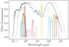 |
Fig. 1 Filter curves of the assembled multi-wavelength data set (coloured lines), overlaid with a galaxy template from Smith et al. (2012). The SED has been normalised to have a peak flux of 1, and it is shown both at z = 0 (in grey) andwith the wavelength axis shifted to z = 1 (in silver) to give the reader an impression of how the excellent multi-wavelength coverage in ELAIS-N1 samples a galaxy’s SED. |
2.2 Sample definition
To avoid thepossible influence of radio selection on our results (see Appendix B for further details), we begin with a sample identified in the 3.6 μm data from SWIRE. These data are not only very sensitive, but they are also less susceptible to the influence of the dust obscuration that could introduce bias into samples identified at shorter wavelengths. We selected those sources with measured 3.6 μm flux density >10 μJy, approximately equal to the 5σ detection threshold in the SWIRE 3.6 μm data and as recommended on the SWIRE webpages2. We includedonly those sources with the necessary flags in the band-merged catalogue, as recommended in Kondapally et al. (2021), to ensure we used only those sources with the highest-quality photometry, the best wavelength coverage, and the most reliable photometric redshifts3. This leaves us with a parent sample of 142 037 3.6 μm-selected sources at z < 1, where Duncan et al. (2021) show that the photometric redshifts have an average scatter of σNMAD < 0.04(1 + z) and an outlier fraction around 5%4.
2.3 LOFAR data
We used the new deep LOFAR observations of the ELAIS-N1 field (Sabater et al. 2021). They cover an area of 10 deg2 that has an rms below 30 μJy, reaching 20 μJy in the deepest regions, which makes them the most sensitive data in the LoTSS Deep Fields DR1. Although the area covered is significantly narrower than that studied in G18, the 150 MHz data are around five times deeper. Importantly, due to the very high qualityof the multi-wavelength data in this field, more than 97 percent of the sources in the ELAIS-N1 LoTSS 150 MHz catalogue have counterparts in at least one band, which have been reliably identified using a new colour-dependent implementation (Kondapally et al. 2021) of the likelihood ratio method (Sutherland & Saunders 1992; Smith et al. 2011; McAlpine et al. 2012; Nisbet 2018; Williams et al. 2019). We used the Sabater et al. (2021) catalogue total 150 MHz flux densities and uncertainties where they exist; however, for the ~ 91 percent of IRAC sources that are not identified as the counterparts of sources in the 150 MHz catalogue, we used pixel flux densities, specifically the flux density measured in the 150 MHz map at the pixel corresponding to the coordinates of each IRAC source. These values indicate the maximum likelihood estimate of the integrated flux density for sources that are unresolved on the scale of the 6 arcsec LoTSS beam, and they are strongly preferred over aperture photometry in these deep data since they are less susceptible to influence from neighbouring sources. Including these sources is especially important since, although they are not individually detected (in the sense that they have a signal-to-noise ratio (S∕N) < 3), they are numerically dominant and together can provide significant diagnostic power, as we shall demonstrate. To limit the potential influence of IRAC sources with 150 MHz emission more extended than 6 arcsec, we only considered the 130 689 sources at z > 0.05. The Kondapally et al. catalogue includes size information for sources in the χ2 image used for source detection, which we have used to estimate the extent of the sources in our sample. The mean full width at half maximum (FWHM) of galaxies along their major axes decreases from 2.7 arcsec at the lowest redshifts to around 1.2 arcsec by z = 1. In practice, therefore, this cut does not have a significant impact on our results since > 99.5% of z < 1 sources – and >98% even at z < 0.2 – have an FWHM smaller than 6 arcsec in the multi-wavelength data. We also include 150 MHz flux density uncertainties measured from the corresponding pixel of the rms map.
2.4 SFR and mass estimation
We used thepanchromatic energy balance SED fitting code MAGPHYS to fit the multi-wavelength matched-aperture photometry and determine the physical properties of each source. MAGPHYS is fully described in da Cunha et al. (2008), but to summarize: it uses an energy balance criterion to link the stellar emission that dominates at optical and near-infrared (ONIR) wavelengths with the dust emission that dominates in the far-infrared. The stellar emission is modelled using the templates from Bruzual & Charlot (2003) and assuming an initial mass function (IMF) from Chabrier (2003), attenuated using a two-component dust model from Charlot & Fall (2000); the energy absorbed is then re-radiated using a multi-component dust model (including dust grains of various sizes and temperatures, as well as polycyclic aromatic hydrocarbons). The energy balance criterion is used to combine an ONIR library based on 50 000 SEDs, which represent exponentially declining star-formation histories with stochastic bursts superposed, with a library of 50 000 dust SEDs with a realistic range of physical properties. The energy balance criterion is designed to ensure that only physical combinations of the stellar and dust SEDs are used to model the input photometry. MAGPHYS does not account for possible additional dust heating due to AGN (though see e.g. Berta et al. 2013, for an attempt to include it). As well as producing best-fit SEDs for every source, we also obtained best-fit physical parameters with marginalised probability distribution functions (PDFs) for each parameter. These PDFs were used to derive median-likelihood parameter estimates (which are the values corresponding to the 50th percentile of the PDF) as well as the 16th and 84th percentiles, which are equivalent to the ± 1σ values for each parameter in the limit of Gaussian statistics.
Since the multi-wavelength data over the ELAIS-N1 field have been compiled from a wide range of sources with different coverage (see Sect. 2.1), not every source has measured photometry in every band. Table 1 shows the fraction of sources in our sample that have coverage and/or a ≥ 3σ detection in each band, while Table 2 shows the fraction of sources that have measured photometry and ≥ 3σ detections in at least N photometricbands. While Table 1 highlights that 100% of our sample have Herschel coverage, only ~ 15% are detected at ≥ 3σ in the most-sensitive 250 μm band, with 22% ≥ 2σ and 43% ≥ 1σ. Indeed, only ~65% of the sample have been assigned Herschel photometry by XID+; the fact that the remaining 3.6 μm sources were not assigned any measurable Herschel flux density, despite the absence of an SED prior in the version of XID+ we used (cf. Pearson et al. 2017), is a strong indication that they are fainter than the confusion noise in each of the Photodetector Array Camera and Spectrometer (PACS) and SPIRE bands (Hurley et al. 2017). To include this “upper limit” information in the MAGPHYS parameter estimation, we assigned these sources uncertainties in the PACS and SPIRE bands equal to the median uncertainty for the sources that do have measured flux densities (these values are 10.3, 14.1, 2.6, 2.8, and 3.7 mJy in the 100, 160, 250, 350, and 500 μm bands, respectively), alongside a small flux density (equal to 0.1% of the median uncertainty)5.
The principal quantities of interest for this work are the stellar mass and the SFR averaged over the last 100 Myr, forwhich MAGPHYS estimates have been shown to be reliable in a range of different situations (e.g. Hayward & Smith 2015; Smith & Hayward 2018; Dudzevičiūtė et al. 2020). To ensure that the MAGPHYS parameters are as reliable as possible, we further refined our sample to include only those 123 425 galaxies for which MAGPHYS has been able to produce an acceptable fit. We define “acceptable” to mean that the χ2 parameter that compares the goodness of the fit between the model and the observed photometry is below the 99 percent confidence threshold derived for the number of bands of photometry available for each object, as discussed in Smith et al. (2012). Though we are unable to repeat their emission line classification, our sample is roughly a factor of eight larger than the one used by G18. In addition, the multi-wavelength data set is far better; the HSC i-band data in ELAIS-N1 are four magnitudes deeper (and the comparison is similar in the other HSC bands), while the IRAC 3.6 μm data are >20 times as sensitive as the closest comparable band in that work. Not only are the individual observations more sensitive, but there are also many more bands of photometry available for us to use. We demonstrate this in Table 2, which shows that more than half of our sample has photometry in 23 or more bands, as compared to the maximum of 14 that were available in the H-ATLAS NGP area used by G18.
Percentage of the area covered in this study by each set of ancillary data used for the SED fitting, along with the mean percentage of sources detected at ≥ 3σ in the most sensitive band of each data set.
Percentage of sources in our parent sample with measured photometry (middle column) and a ≥ 3σ detection in at least N bands.
2.5 Sample properties and AGN contamination
As recommended by Duncan et al. (2021), we removed: (a) the most obvious AGN in our mass-selected sample using the flags supplied in the input catalogue, which include sources in the Million Quasar Catalog (Flesch 2019) and sources spectroscopically classified as AGN in the literature, (b) those sources that fall into the Donley et al. (2012) infrared colour space dominated by AGN, and (c) those with bright X-ray counterparts (see Duncan et al. 2021 for details); this left us with 122 646 sources. However, for those galaxies with 150 MHz detections, we also removed additional AGN that were identified using the method from Best et al. (in prep.), which relies on the results of a comprehensive multi-wavelength SED fitting analysis, using our MAGPHYS results alongside those derived using BAGPIPES (Carnall et al. 2018), AGNFITTER (Calistro Rivera et al. 2016), and CIGALE (Burgarella et al. 2005). The details of the Best et al. method are complex, but the general idea is to compare the results of those SED fitting codes that account for AGN (AGNFITTER and CIGALE) with those that are focussed on normal star-forming and passive galaxies (MAGPHYS and BAGPIPES) considering all of the available information including comparing the goodness-of-fit that each code produces, accounting for the best-fit AGN fractions, and identifying sources with a clear radio excess. A comparison between the Best et al. (in prep.). AGN flagging procedure and the results of removing the bad MAGPHYS fits using the aforementioned χ2 threshold method from Smith et al. (2012) suggests that applying the MAGPHYS threshold alone removes ~ 96 percent of the flagged AGN. This is especially useful for this work since the Best et al. (in prep.) AGN flags have only been derived for the sources detected in the 150 MHz catalogue6. After applying these cuts, we were left with 120 232 z < 1 galaxies, of which 9298 (25 777) are detected at ≥5σ (≥3σ) in the deep LoTSS data. We also identified 1715 further sources that were not flagged as AGN in the Best et al. radio excess sample but which had a clear radio excess in our pixel flux density measurements (> 5σ 150 MHz detections and L150 MHz more than 1 dex larger than the SFR-L150 MHz relation from G18; this is 1.4 percent of our sample), which indicates they are likely undiagnosed AGN; we thus removed them from our sample, leaving us with 118 517 galaxies on which to base our analyses. We repeated the analyses and note that the results did not significantly change regardless of whether or not we included these sources, whether or not we used a 1 dex excess or a 0.7 dex radio excess to identify residual AGN, or whether or not we instead used the mass-dependent SFR-L150 MHz relation from G18.
Histograms showing the median-likelihood SFR, stellar mass, redshift, and 150 MHz S/N distribution for the galaxies in our sample are shown in Fig. 2. In Fig. 3, we display the stellar mass (top) and SFR (bottom) distributions as a function of redshift, colour-coded by the number of galaxies in each bin.
In Fig. 4, we show the location of the SFR and 150 MHz luminosity for those 25 777 sources that are detected at > 3σ in the deep LoTSS data, overlaid with the mass-independent SFR-L150 MHz relation (orange line) and broken power-law parameterisation (dashed blue line) found by G18 (which was based on a sample identified based on the MPA-JHU catalogue at optical wavelengths). The apparent offset to larger L150 MHz in this sample relative to the G18 relations is an artefact of the data having been censored by the 3σ threshold in L150 MHz, and it does not account for the large majority of sources in our sample that fall below it. The formally non-detected (i.e. < 3σ) radio sources have huge potential diagnostic power due to their numerical dominance (e.g. Zwart et al. 2015; Malefahlo et al. 2020), but they are challenging to visualise in the SFR-L150 MHz plane. As the lower-right panel of Fig. 2 shows, the vast majority of sources in our IRAC-selected sample have 150 MHz flux densities with <3σ significance, and a substantial minority have negative measured flux densities. It is critical that we also account for these sources since failure to do so clearly truncates the luminosity distribution at a given SFR, and, left unchecked, this would have the potential to introduce significant bias into our results.
Finally, to test the possible influence of sample incompleteness on our results, we used the method from Pozzetti et al. (2010) to identify those galaxies with masses in excess of the 95% mass completeness limit as a function of redshift (shown as the dashed blue line in the upper panel of Fig. 3). We repeated all of the following analyses considering only those galaxies with masses in excess of the 95% completeness limit and found that our results did not change when the uncertainties were taken into account. We therefore conclude that incompleteness does not exert significant influence on our results.
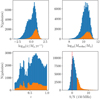 |
Fig. 2 Histograms (clockwise from the top-left) showing the SFR (ψ), stellar mass, 150 MHz S/N, and redshift distributions for the 118 517 galaxies in our 3.6 μm-selected z < 1 sample after applying the cuts discussed in Sect. 2. The overlaid orange histograms show the corresponding distributions for the subset of the sample that is detected to ≥ 3σ at 150 MHz. |
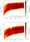 |
Fig. 3 Heatmaps showing the variation in median-likelihood stellar mass in M⊙ (top) and SFR (ψ) in units of M⊙ yr−1 (bottom) as a function of redshift in our IRAC-selected sample. The redshift axis is common to both plots, and the number of galaxies in each bin is indicated by the colour scales to the right. Upper panel: the dashed blue line indicates the 95% mass completeness limit as a function of redshift, derived using the method from Pozzetti et al. (2010). |
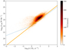 |
Fig. 4 SFR-L150 MHz plane populated by the 25 777 sources with ≥3σ detections in the 150 MHz data, with the colour bar to the right indicating the bin occupancy. The best-fit relations from G18 are overlaid for comparison; the mass-independent relation is shown in orange, while the broken power-law relation evaluated at 1010 M⊙ is shown as the dashed blue line. |
3 Results
3.1 The SFR-L150 MHz relation
We determined the SFR-L150 MHz relation in ELAIS-N1, while accounting for uncertainties on both SFR and L150 MHz, as follows. First, for each source in our sample, we created a two-dimensional PDF in the SFR-L150 MHz parameter space with logarithmic axes in both directions, with 70 equally spaced bins of SFR between − 3 < log10(ψ∕M⊙ yr−1) < 3 and 180 equally log-spaced bins of L150 MHz between 17 < log10 (L150 MHz∕W Hz−1) < 26. We generated each source’s PDF by creating a histogram using the aforementioned bins, populated by 100 samples each in the SFR and L150 MHz directions, assuming that the uncertainties in SFR and L150 MHz are uncorrelated. For the L150 MHz values, we adopted a normally distributed error distribution (in linear space) with median and standard deviation equal to those derived using the measured flux densities and an rms from the LoTSS data at each source’s redshift in our adopted cosmology. To ensure that the low signal to noise and negative values of L150 MHz are included in the PDF – essential to avoid biasing them by censure – we arbitrarily assigned samples with log10L150 MHz < 17 (including the negative values) to the lowest bin of the L150 MHz PDF. For the SFRs, we adopted an asymmetric error distribution with a median equal to the median-likelihood value of the MAGPHYS SFR PDF, and a different standard deviation on either side of the median, equal to the difference between the 84th (16th) and 50th percentiles of the SFR PDF for the positive (negative) wings of the error distribution. We then summed these PDFs over the whole sample to arrive at a stacked PDF showing the distribution of SFR and L150 MHz that includes the uncertainties for the whole sample in both directions. This is shown as the heatmap in the background of Fig. 5, with the colour bar to the right indicating the number of galaxies in each bin7.
One of the most interesting results from G18 was the discovery of an upturn in the SFR-L150 MHz relation at low SFRs, below log10 (ψ∕M⊙ yr−1) ≈ 0, and the G18best-fit broken power-law relation is shown as the dashed blue line in Fig. 5 (for a stellar mass of 1010 M⊙, typical of galaxies in our sample). In order to identify the SFR-L150 MHz relation in our data, we used a non-parametric approach. Non-parametric methods have the implicit advantage of being agnostic about the precise formof any relation that they may recover, and are therefore ideal for determining whether the data support an upturn at a low SFR, of the type seen in G18, or not. At each SFR, we calculated the 16th, 50th, and 84th percentiles of the L150 MHz distribution in the stacked two-dimensional PDF. The 50th percentile of the distribution then corresponds to our median-likelihood estimate of the SFR-L150 MHz relation at that particular SFR, while the 16th and 84th percentiles also depend on the combination of the uncertainties on the luminosity estimates, plus any intrinsic scatter in the relation itself. We estimated the uncertainties on the median-likelihood value in each SFR bin by using the median statistics method from Gott et al. (2001). A further appealing feature of a median-likelihood estimate is that it has a degree of built-in resistance to outliers, such as might be expected from, for example, some residual minority of sources hosting unidentified radio excess due to AGN activity. We also note that deriving the best-fit relation in this way does not require us to account for the intrinsic dispersion of the relation itself, σL, to which we will return in Sect. 3.2.
The results are shown as the red lines overlaid on Fig. 5, with the thick line corresponding to the median-likelihood estimate of SFR-L150 MHz over the range − 2 < log10(ψ∕M⊙ yr−1) < 2, with the 16th and 84th percentiles shown as the thin red lines. It is immediately clear that the median-likelihood relation is similar to the mass-independent relation found by G18, albeit slightly flatter, and that the recovered values appear consistent with a power-law relationship across the full range of the SFRs spanned by our sample, with no evidence of an upturn in L150 MHz at low SFRs. To determine the best-fit parameters, we adopted the form of the SFR-L150 MHz relation from G18, specifically
 (1)
(1)
and find best-fit values of log10L1 = 22.181 ± 0.005 and β = 1.041 ± 0.007, where the uncertainties have been determined using the emcee (Foreman-Mackey et al. 2013) Monte Carlo Markov chain (MCMC) algorithm with 16 walkers and a chain length of 10 000 samples.
In Appendix C, we present a suite of simulations conducted to test how well we can recover a known SFR-L150 MHz relation using this method, and we find that the best-fit estimates are likely to be systematically offset by Δ log10L1 ≈ 0.040 and Δβ ≈ 0.016. Correcting for these effects gives our best estimate of the overall SFR-L150 MHz relation, which is log10L150 MHz = (22.221 ± 0.008) + (1.058 ± 0.007)log10(ψ∕M⊙ yr−1). Although these values are formally inconsistent with the results from G18 (i.e. log10L1 = 22.06 ± 0.01, β = 1.07 ± 0.01), the fact that they are this close is encouraging, given the large differences in methodology and sample definition.
Figure 5 shows a clear offset between the apparent peak of the stacked PDF (background colour scale) and the median-likelihood values (thick red lines), which corresponds to our estimate of the SFR-L150 MHz relation. This effect results from sampling linear L150 MHz values in a logarithmic PDF, which means that the lower half of the PDF is effectively spread out over a larger number of bins compared to the higher half 8. This effect is also clearly apparent in the simulations of our method discussed in Appendix C, which underlines that the non-Gaussianity in the PDF does not stop the median-likelihood values (of the individual sources and of the population) from being able to recover the true SFR-L150 MHz relation.
The third important thing to notice about Fig. 5 is that the 16th percentile of the L150 MHz distribution (shown as the lower red line) rapidly decreases below the bottom of the plotting window at log10ψ < 0.7. This highlights the importance of including the formally undetected sources in this study (i.e. those with 150 MHz flux density < 3σ), and this importance of course increases as we move to lower SFRs, where an increasing fraction of objects have 150 MHz flux densities below 1σ. The simulations discussed in Appendix C further highlight the importance of accounting for the negative L150 MHz samples since not doing so would introduce significant positive bias into the median flux density.
It is tempting to also determine the SFR-L150 MHz relation by finding the “ridge-line” in the stacked two-dimensional PDF that corresponds to the modal value of L150 MHz at a given SFR. If we do this, we obtain good agreement with the above median-likelihood estimates at log10(ψ ∕ M⊙ yr−1) > 1; however, as we move to lower SFRs, we begin to see positive bias introduced, similar to the upturn seen in G18. This is another facet of the aforementioned issue with increasingly sampling the noise distribution as we move to lower SFRs: if all sources were at the same redshift, then we are effectively attempting to plot a histogram of the logarithm of a normal distribution in luminosity that is centred very close to zero, and the ridge-line becomes increasingly biased.
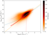 |
Fig. 5 Stacked heatmap showing the two-dimensional PDF for SFR and L150 MHz for all 118 517 galaxies in our sample, including the uncertainties on the SFR (derived based on the percentiles of the MAGPHYS SFR PDF) and on L150 MHz (using the pixel flux densities and rms values at the redshift in the Duncan et al. 2021 catalogue). The “effective” number of galaxies in each bin – we recall that each galaxy is sampled 100 times (with each sample representing 0.01 galaxies) and can therefore contribute to multiple pixels in the stack – is indicated by the colour bar to the right. The best-fit SFR-L150 MHz relationship from G18 is overlaid as the solid orange line, along with the broken power-law G18 relation (which we have evaluated at a canonical stellar mass of 1010 M⊙, and which is shown as the dashed blue line) along with (in red) the 16th, 50th, and 84th percentiles of the L150 MHz distribution at each SFR. |
3.2 Scatter on SFR-L150 MHz
In addition to the form of the SFR-L150 MHz relation, it is also of interest to determine the scatter on the relation itself, σL, which is usually quoted in logarithmic terms (dex). Whatever the cause, σL is important since it forms a key part of the process of identifying AGN in 150 MHz samples on the basis of an SFR-dependent radio excess (Best et al., in prep.). It is also of interest when studying the so-called “main sequence” of star formation – the relationship between the stellar mass and SFR of star-forming galaxies (e.g. Noeske et al. 2007; Johnston et al. 2015; Schreiber et al. 2015) – using radio observations (e.g. Leslie et al. 2020). The width of the main sequence has been interpreted as a manifestation of the variation in a star-forming galaxy’s gas supply (Tacchella et al. 2016); therefore, an additional source of scatter in the SFR indicator itself has the potential to bias the results if it is not measured and accounted for.
To measure the scatter on the SFR-L150 MHz in our data, we used Monte Carlo simulations. We did this by creating multiple realisations of our sample, using the best-fit redshifts alongside random draws from the MAGPHYS SFRs (assuming the same asymmetric error distribution as in Sect. 3.1) and from the best-fit relation (Eq. (1)), with a scatter in the range 0.0 < σL < 0.5 dex, to calculate a model L150 MHz for each source. We used these values to derive “true” flux densities and simulate measurement errors based on realisations of the values in the rms map at the position of that source in the real data. For each simulation, we conducted two-sample Kolmogorov-Smirnov (KS) tests to compare the model flux densities with the real flux density distribution for any choice of SFR and redshift, to in turn determine the degree of support for the hypothesis that the simulated flux densities are consistent with being drawn from the same distribution as the real values, as a function of σL. Figure 6 shows the true pixel flux density distribution in red, overlaid on one set of Monte Carlo simulations covering the full range in scatter (shaded grey). The individual grey histograms are transparent, such that lighter grey regions reveal the variation in the flux density distribution for the range of scatter considered. Following Macfarlane et al. (2020), we truncated the distribution above a flux density of 1 mJy to avoid giving undue influence to residual undiagnosed AGN in our sample (this does not make a significant difference to the results). We determined the mean P returned by the KS test (averaging over all 10 000 Monte Carlo simulations) as a function of σL and marginalised the resulting distribution. We were then able to calculate median-likelihood estimates of σL along with uncertainties by estimating the 16th, 50th, and 84th percentiles of the PDF, as well as Bayesian estimates calculated according to ∑ σLP(σL).
Figure 7 shows our results from using the KS tests to determine the level of support in the data for different values of σL as a function of SFR in bins with a constant width of 1 dex in SFR on a sliding scale from − 2< log10(ψ∕M⊙ yr−1) < 2. We only detect significant scatter about SFR-L150 MHz at log10(ψ∕M⊙ yr−1) > 0, with σL apparently increasing with SFR and reaching 0.31 ± 0.01 dex at 1< log10(ψ∕M⊙ yr−1) < 2. This may be because the scatter in the flux density distribution is increasingly dominated by the sensitivity of the LOFAR observations as we approach lower SFRs, rather than by the physical effect that is most visible at larger SFRs. It will be of great interest to see whether this effect persists with larger samples of log10(ψ∕M⊙ yr−1) < 0 galaxies from the wider-area LoTSS second data release once it is available, and in due course with the huge increase in sensitivity that the SKA will provide.
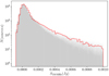 |
Fig. 6 Histogram with logarithmic ordinates, showing the true observed flux density distribution (in red) overlaid on individual Monte Carlo realisations (shown in grey with transparency, such that lighter shading indicates the range of outputs) based on assuming the best-fit SFR-L150 MHz relation from Sect. 3.1 with the full range of intrinsic scatter 0.0 < σL < 0.5. |
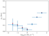 |
Fig. 7 Variation in median-likelihood estimates of σL as a function of the central value of each SFR bin. The error bars in the vertical direction are derived from the 16th and 84th percentiles of the PDF, while in the horizontal direction the error bars indicate the bin width. Also overlaid are red circles, indicating the Bayesian estimates of scatter from the PDF, calculated according to the product of Σ σLP (σL). |
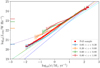 |
Fig. 8 Median-likelihood estimates of the SFR-L150 MHz relation for the wholesample (red circles) and in four redshift bins (0.05 < z < 0.30, 0.30 < z < 0.60, 0.60 < z < 0.80, and 0.80 < z < 1.00 are shown as the blue, orange, green, and red crosses, respectively). Error bars on the median L150 MHz are calculatedusing the median statistics method from Gott et al. (2001). Also overlaid are the SFR-L150 MHz relationships from Bell (2003, dot-dashed purple line) and Murphy et al. (2011, dashed cyan line), converted to 150 MHz assuming a canonical spectral index α = 0.7, and the 150 MHz relations from G18 (mass-independent shown as the solid orange line, broken power law evaluated at 1010 M⊙ as the dashed purple line) and Wang et al. (2019) (shown as the dotted blue line). The literature calibrations have been converted toour adopted IMF from Chabrier (2003) using the factors recommended in Madau & Dickinson (2014). The horizontal coloured lines immediately to the right of the left-hand vertical axis indicate the luminosity corresponding to the 60 μJy at the lower redshift bound of each bin, as indicated by the colour (see text for details). |
3.3 Evolution of SFR-L150 MHz and σL
In order to investigate the possibility of evolution in the derived properties of SFR-L150 MHz, we split the sample into four redshift bins and repeated the analysis from the previous two sections. Figure 8 shows the median-likelihood SFR-L150 MHz derived over the full redshift range (in red) and overlaid with the values derived for each redshift bin (coloured as in the legend). For the purposes of comparison, we have once again overlaid the G18 relation (in orange) as well as the empirical relations from Bell (2003) and Murphy et al. (2011), both converted from the 1.4 GHz expectations assuming a canonical spectral index of α = 0.7 (similar to values in the literature, e.g. Mauch et al. 2013; Prescott et al. 2016), and the relation from Wang et al. (2019). All of these literature relations have been converted to the Chabrier (2003) IMF used in this work where necessary, using the corrections provided in Madau & Dickinson (2014). To indicate the flux density scale in each redshift bin, we have also overlaid horizontal coloured lines adjacent to the left-hand vertical axis, which indicate values of L150 MHz corresponding to 60 μJy (i.e. the approximate3σ limit in the deepest regions of the 150 MHz data) at the lowest redshift bound of each bin (indicated by the colour of the line).
At log10 (ψ∕M⊙ yr−1) > 1, there is negligible difference apparent between the SFR-L150 MHz relation derived over the full redshift range and the values in each redshift bin. However, at log10(ψ∕M⊙ yr−1) < 1, there is the first piece of evidence of variation and perhaps evidence of an excess in radio luminosity that increases towards the lowest SFR end of the data sampled in each redshift range, where the individual galaxies’ 150 MHz flux densities are formally undetected. To determine whether this effect is real or instrumental, we conducted further simulations, repeating the analysis using a known input SFR-L150 MHz relation, sampling the observed z and SFR distributions and uncertainties alongside a realistic model for mass-dependent AGN contamination following Sabater et al. (2019), and modelling the effects of noise in the 150 MHz flux densities by sampling from the real data set. The simulations are discussed in further detail in Appendix C. We were unable to reproduce variations in SFR-L150 MHz, such as the possible upturn seen at log10(ψ∕M⊙ yr−1) < 1 using a mass-independent SFR-L150 MHz relation of the form given by Eq. (1). If this effect is real, it may point to possible mass dependence in SFR-L150 MHz as found by G18. We will return to this topic in Sect. 3.4.
To make a better comparison with G18, who used a z < 0.3 sample that was defined based on SDSS spectroscopy, we also derived best-fit parameters for the corresponding redshift range in our sample (our lowest redshift bin). We find best-fit parameters of log10L1 = 22.14 ± 0.01 and β = 1.22 ± 0.01, corrected for residual bias in the same way as in Sect. 3.1. Although our z < 0.3 L1 estimate is comparable, the value for β that we obtain in the lowest redshift bin is significantly steeper than that from G18, who found L1 = 22.06 ± 0.01 and β = 1.07 ± 0.01. As mentioned in Sect. 3.1, there are significant differences in the methodology used by the two works, especially the selection function, meaning that we are not necessarily comparing like with like.
We also searched for evidence of evolution in the scatter using the same method as in Sect. 3.2, but limiting the SFR range to 0.5 < log10(ψ∕M⊙ yr−1) < 1.5 (to mitigatepossible variation in scatter over SFR) and limiting the stellar mass range to 10 < log10(M∕M⊙) < 11 (to mitigate any possible influence of the mass dependence in SFR-L150 MHz found by G18), using the same redshift bins as above. In Fig. 9, we plot the derived values as a function of redshift, along with their error bars. While some variation in σL is possible within the uncertainties, the data do not show any evidence for linear evolution in σL, at least out to z = 1.
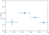 |
Fig. 9 Variation in σL for galaxies with 0.5 < log10ψ < 1.5, 10 < log10(M∕M⊙) < 11 as a function of redshift – with error bars derived from the 16th and 84th percentiles of the PDF – and centred on the median-likelihood values. The error bars in the redshift (horizontal) direction indicate the bounds of each redshift bin. |
3.4 Mass dependence of SFR-L150 MHz
Finally, we also considered the possibility of stellar mass dependence in SFR-L150 MHz as discussed by G18 and Read (2019, and in prep.). To do this, we introduced a three-dimensional version of the method we used in Sect. 3.1, now producing 100 samples in each of the SFR, stellar mass, and L150 MHz directions to make a three-dimensional PDF for each source. Once again, we accounted for possible asymmetry in the SFR and stellar mass error bars by using the 16th, 50th, and 84th percentiles of the MAGPHYS estimates and sampling from a linear space in the uncertainty on L150 MHz. As before, we then summed over all 118 517 sources in our sample. We used 50 equally spaced logarithmic bins of stellar mass between 7.5 < log10(M∕M⊙) < 11.8, 60 equally spaced logarithmic bins of SFR between − 3 < log10(ψ∕M⊙ yr−1) < 3, and 180 equally spaced logarithmic bins of L150 MHz between 17 < log10(L150 MHz∕W Hz−1) < 26 to calculate the median-likelihood L150 MHz in each bin. The left-hand panel of Fig. 10 shows values of median-likelihood L150 MHz as a function of the SFR at a constant stellar mass indicated by the colour bar, effectively slicing through our three-dimensional stellar mass–SFR–L150 MHz distribution. Similarly, the right-hand panel shows corresponding values of L150 MHz as a function of stellar mass at a fixed SFR (with the SFR indicated for each line by the colour bar). In both panels, we show only those bins populated by at least 15 galaxies (after accounting for the fact that each galaxy is sampled 100 times), though there are still some effects of small number statistics visible in the lowest SFR bins, particularly in the right-hand panel. Nevertheless, the left-hand panel reveals a variation of at least 0.5 dex in L150 MHz for a given SFR, depending on the stellar mass, while the right-hand panel shows more than 2 dex of SFR-dependence in L150 MHz at a fixed stellar mass. These effects are clearly large enough to potentially account for the difference in SFR-L150 MHz that we observe in our lowest redshift bin relative to G18, and which we discussed in Sect. 3.3.
To quantify our results, we used the mass-dependent parameterisation from G18:
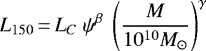 (2)
(2)
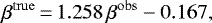
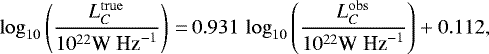
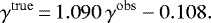
and obtain best-fit values of log10LC = 22.111 ± 0.004, β = 0.850 ± 0.005, and γ = 0.402 ± 0.005, where G18 obtained log10LC = 22.13 ± 0.01, β = 0.77 ± 0.01, and γ = 0.43 ± 0.01. We conducted an additional set of simulations, which we discuss in Appendix C, to determine how well we are able to recover a known relation of the form given by Eq. (2). We find that, using this method, the best-fit estimates are likely to be offset by a residual bias of Δβ = 0.053, Δ log10LC = 0.107, and Δγ = −0.072, giving best estimates of β = 0.903 ± 0.012, log10LC = 22.218 ± 0.016, and γ = 0.332 ± 0.037 where we have propagated the uncertainties based on the systematic corrections by adding in quadrature with those values derived from our MCMC fitting.
To visualise the improvement in accuracy resulting from Eq. (2), we show in Fig. 11 the same data as in Fig. 10, but with the mass and SFR dependency taken out (in the left- and right-hand panels, respectively) using the best-fit parameters from Eq. (2). Together, these plots reveal compelling evidence for mass dependence in SFR-L150 MHz, in the sense that more massive galaxies have a larger radio luminosity at a fixed SFR. The fact that the mass dependence appears constant, and that it is clearly evident even in galaxies with stellar masses below 1010 M⊙, suggests that it is unlikely to be caused by some undiagnosed AGN contamination, given the mass dependence in AGN fraction shown by Sabater et al. (2019), for example.
Interestingly, we repeated the Monte Carlo simulations discussed in Sect. 3.2 to see whether assuming a mass-dependent SFR-L150 MHz relation and including the MAGPHYS stellar mass information in the simulations made any difference to our measurements of σL. The results on both the SFR and redshift dependence in σL are consistent within the uncertainties whether we use a mass-dependent or mass-independent SFR-L150 MHz, suggesting that mass dependence – at least as parameterised in Eq. (2) – cannot explain the scatter on SFR-L150 MHz.
We also used a mass-dependent SFR-L150 MHz relation as an input to the simulations discussed in Appendix C.1 and find that it allows us to recover an excess L150 MHz at low SFRs, very similar to the possible excess observed in the redshift bins of Fig. 8. Mass dependence on SFR-L150 MHz may therefore beable to explain the possible variation revealed in Fig. 8, and it may also provide an explanation for the radio excess apparent at low SFRs first noticed by G18. We intend to revisit this issue in a future work.
4 Discussion and conclusions
We have studied the relationship between SFRs and 150 MHz luminosity using new sensitive deep field observations from the LoTSS Deep Fields DR1. Starting from a near-infrared selected sample, we leveraged the multi-wavelength aperture-matched forced photometry and state-of-the-art photometric redshifts, alongside the new LoTSS maps of the ELAIS-N1 field, to produce stellar mass and SFR estimates using energy balance SED fits with the MAGPHYS package. We used 150 MHz flux densities from the ELAIS-N1 catalogue, plus pixel flux densities for the remaining 109 206 IRAC sources that are not identified as counterparts to catalogued 150 MHz sources, to estimate the median-likelihood L150 MHz as a function of the SFR and stellar mass.
The 150 MHz data used in this study are five times more sensitive than those used by G18, the sample size is eight times larger, and the multi-wavelength coverage in this field is far superior. This is true both in terms of depth (e.g. the HSC i-band data over ELAIS-N1 reach a 5σ magnitude fainter than 26 mag, around four magnitudes deeper than the SDSS imaging used in G18) and in terms of the number of photometric bands that are available (Table 2 reveals that more than half of our sample have ≥ 3σ flux densities in at least 16 bands, as compared to a maximum of 14 in G18). The LoTSS deep field data in ELAIS-N1 are around 35 times deeper than the FIRST data that have been used for previous studies of this topic (e.g. Hodge et al. 2008; Garn et al. 2009; Davies et al. 2017), assuming a standard canonical spectral index value of α = 0.7; they are comparable to the deepest degree-scale interferometric radio data in existence (e.g. Smolčić et al. 2017) but cover an area of sky five times larger.
Using a non-parametric approach, we find an apparently linear relationship between the SFR and L150 MHz over the range in SFR − 2 < log10(ψ∕M⊙yr−1) < 2 of the form L150 MHz = L1ψβ, with best-fit parameters equal to log10L1 = 22.221 ± 0.008 and β = 1.058 ± 0.007. We find an SFR-dependent scatter about the SFR-L150 MHz relation, reaching σL ≈ 0.31 ± 0.01 dex at 1 < log10(ψ∕M⊙ yr−1) < 2. Our inability to detect significant scatter at lower SFRs log10(ψ∕M⊙ yr−1) < 0 may be a limitation of the sensitivity in the 150 MHz data, even though they are the deepest in existence. Neither the scatter nor the high-SFR end (log10(ψ∕M⊙ yr−1) > 1) of the best-fit relation show significant evidence for redshift evolution, with the latter found to be in agreement with, for example, Garn et al. (2009) and Duncan et al. (2020), out to larger SFRs and redshifts. Our results also agree with Calistro Rivera et al. (2017, who used a 150 MHz and i-band selected sample) out to our z < 1 limit, though they do see evidence for evolution in SFR-L150 MHz in more distant sources.
The (close to) unitary slope that we determine for the best-fit SFR-L150 MHz relation is apparently consistent with expectations based on calorimetry models (e.g. Chi & Wolfendale 1990; Yun et al. 2001; Lacki et al. 2010), and it is similar to previous low-frequency results (e.g. Brown et al. 2017, who found β = 1.14 ± 0.05, and G18, who found β = 1.07 ± 0.01). However, like G18 and Read (2019), we find a clear mass dependence in the SFR-L150 MHz relation, in the sense that higher mass galaxies have a larger L150 MHz at a fixed SFR. Our best-fit mass-dependent relation is log10L150 MHz = (0.90 ± 0.01)log10 (ψ∕M⊙ yr−1) + (0.33 ± 0.04)log10(M∕1010M⊙) + 22.22 ± 0.02. Using a suite of realistic simulations, we have shown that the mass dependence can explain the possible observed deviation from linearity in the redshift-binned SFR-L150 MHz relation, as well as potentially the radio excess in low-SFR galaxies found by G18. This implies that the unitary slope we recovered in the overall SFR-L150 MHz may be a coincidence, and – assuming direct proportionality in the relationship between the far-infrared luminosity and the SFR as described, for example, in Kennicutt & Evans (2012) – we expect to observe similar mass dependence in the FIRC.
One possible explanation for these results could be a mass-dependent cosmic ray escape fraction that allows particles to remove energy from the galaxy before it can be radiated away at radio frequencies, especially in lower mass (smaller) galaxies. However, it is also important to consider whether undiagnosed AGN contamination can play a role since a radio excess that increases with growing stellar mass would be in keeping with previous results on the massdependence of the AGN fraction (Sabater et al. 2019). However, the mass dependence apparent in our data is clear and consistent across the whole sample, including in galaxies with stellar masses below 1010 M⊙, implying that it is unlikely to be due to undiagnosed AGN contamination. At the same time, we are unable to rule out the presence of undiagnosed AGN in our sample altogether, especially low-excitation systems (which manifest as a large accretion-related radio excess but with little or no evidence for AGN in the multi-wavelength SED, e.g. Hardcastle et al. 2007; Best & Heckman 2012), but this type of undiagnosed AGN is unlikely to explain our results. Such issues relating to mass dependence are also discussed by Molnár et al. (2018) in the context of a variation in the FIRC in bulge-dominated galaxies (which also tend to be more massive than pure disk-dominated systems). We defer a more detailed discussion of this aspect of our results to a future work.
Irrespective of the cause, the size of this trend is such that failing to account for the stellar mass dependence can introduce systematic offsets on 150 MHz-derived SFRs, with a magnitude around 0.5 dex in either direction (consistent with the results shown in Read 2019), which are therefore potentially larger than the scatter inherent in SFR-L150 MHz. This value is also large enough that mass effects may explain the redshift evolution in the SFR-L150 MHz relation found by Calistro Rivera et al. (2017), although it is also possible that the evolution they report is partly due to their selection function (as underlined by our tests in Appendix B) and/or is only detectable at the higher redshifts probed by that work.
We continue to obtain new 150 MHz data over the ELAIS-N1 field, with the ultimate goal of reaching another factor of two greater sensitivity over the coming years. Complete optical spectroscopy using the William Herschel Telescope Enhanced Area Velocity Explorer (WEAVE: Dalton 2016) instrument will be obtained for every ELAIS-N1 150 MHz source brighter than 100 μJy as part of the WEAVE-LOFAR survey (Smith et al. 2016), which is scheduled to begin in the second quarter of 2021. Over five initial years of survey operations, WEAVE-LOFAR will obtain around a million spectra of LOFAR-selected sources in the best studied extragalactic fields in the Northern Hemisphere at every scale (ranging from deep fields such as ELAIS-N1, Lockman Hole, and Boötes and covering, for example, the whole of the H-ATLAS NGP field used by G18 and thousands of square degrees at high galactic latitudes), providing precise redshifts for virtually every source placed in a WEAVE fibre at z < 1. These new data will enable the use of extensive emission line classifications and Balmer-decrement derived SFRs to study the SFR-L150 MHz relation, which will in turn enable us to significantly improve on this work, including the full coverage of the luminosity-redshift plane simultaneously sampled by the wide and deep fields with highly uniform spectroscopy.
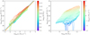 |
Fig. 10 L150 MHz dependence with SFR and stellar mass. Left: SFR-L150 MHz relation as a function of stellar mass, indicated by the colour of the line and relative to the colour bar, overlaid on the mass-independent relation from G18 (solid orange line) and our best-fit estimate from Sect. 3.1 (dashed blue line). Each coloured line shows the median-likelihood L150 MHz at a given SFR and stellar mass. Right: relationship between stellar mass and median-likelihood L150 MHz, coloured as a function of SFR with the scale indicated by the bar to the right. |
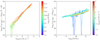 |
Fig. 11 Accounting for stellar mass effects in SFR-L150 MHz. Left: SFR-L150 MHz relationship with the mass dependence taken out using Eq. (2) and the best-fit parameters. Stellar mass is indicated by the colour bar to the right. Right: same as the left, but with the relationship between the stellar mass and radio luminosity normalised by the SFR using Eq. (2). |
Acknowledgements
The authors would like to thank the anonymous reviewer for a positive and constructive report which has improved the quality of the paper. M.J.H. acknowledges support from the UK Science and Technology Facilities Council (ST/R000905/1). R.K. acknowledges support from the Science and Technology Facilities Council (STFC) through an STFC studentship via grant ST/R504737/1. K.J.D. and H.R. acknowledge support from the ERC Advanced Investigator programme NewClusters 321271. I.M. acknowledges support from STFC via grant ST/R505146/1. P.N.B. and J.S. are grateful for support from the UK STFC via grant ST/R000972/1. M.J.J. acknowledges support from the UK Science and Technology Facilities Council (ST/N000919/1) and the Oxford Hintze Centre for Astrophysical Surveys which is funded through generous support from the Hintze Family Charitable Foundation. M.Bo. acknowledges support from INAF under PRIN SKA/CTA FORECaST and from the Ministero degli Affari Esteri della Cooperazione Internazionale – Direzione Generale per la Promozione del Sistema Paese Progetto di Grande Rilevanza ZA18GR02. I.P. acknowledges support from INAF under the SKA/CTA PRIN “FORECaST” and the PRIN MAIN STREAM “SAuROS” projects. This research has made use of NASA’s Astrophysics Data System Bibliographic Services. LOFAR (van Haarlem et al. 2013) is the Low Frequency Array designed and constructed by ASTRON. It has observing, data processing, and data storage facilities in several countries, which are owned by various parties (each with their own funding sources), and that are collectively operated by the ILT foundation under a joint scientific policy. The ILT resources have benefited from the following recent major funding sources: CNRS-INSU, Observatoire de Paris and Université d‘Orléans, France; BMBF, MIWF-NRW, MPG, Germany; Science Foundation Ireland (SFI), Department of Business, Enterprise and Innovation (DBEI), Ireland; NWO, The Netherlands; The Science and Technology Facilities Council, UK; Ministry of Science and Higher Education, Poland; The Istituto Nazionale di Astrofisica (INAF), Italy. This research made use of the Dutch national e-infrastructure with support of the SURF Cooperative (e-infra 180169) and the LOFAR e-infra group. The Jülich LOFAR Long Term Archive and the German LOFAR network are both coordinated and operated by the Jülich Supercomputing Centre (JSC), and computing resources on the supercomputer JUWELS at JSC were provided by the Gauss Centre for Supercomputing e.V. (grant CHTB00) through the John von Neumann Institute for Computing (NIC). This research made use of the University of Hertfordshire high-performance computing facility and the LOFAR-UK computing facility located at the University of Hertfordshire and supported by STFC [ST/P000096/1], and of the Italian LOFAR IT computing infrastructure supported and operated by INAF, and by the Physics Department of Turin University (under an agreement with Consorzio Interuniversitario per la Fisica Spaziale) at the C3S Supercomputing Centre, Italy.
Appendix A Generating stacked PDFs by sampling
To illustratethe way that we created stacked two-dimensional PDFs using random sampling, we have included the following simple example based on two model parameters of interest. We assumed that both parameters have asymmetric uncertainties, but for different reasons. In the case of our first parameter (hereafter “parameter 1”), we assumed uncertainties that are normally distributed in linear space, but we wished to stack the PDF in log space (as in the case for L150 MHz in our real data set). For our second parameter (“parameter 2”), we proceeded as we did for our MAGPHYS estimates of stellar masses or SFRs since the MAGPHYS PDFs generally do not have an analytic form. We therefore made the simplifying assumption that the underlying PDF is Gaussian distributed, and we set the width of the distribution on the positive (negative) side using the difference between the 84th (16th) and 50th percentiles of the MAGPHYS PDF.
The four panels of Fig. A.1a show the PDFs assumed for parameters 1 and 2 in blue and orange, respectively, for some arbitrarily chosen values as well as for the hypothetical case of the four galaxies that we wish to stack. We then generated 100 samples from the assumed PDF for each parameter and for each galaxy; histograms of these samples have been overlaid in Fig. A.1a. Since we assume that the uncertainties are independent, we can use these samples to create a two-dimensional PDF for each object by creating a two-dimensional histogram using the same samples and then normalising. Examples of these two-dimensional PDFs for the four hypothetical objects are displayed in Fig. A.1b.
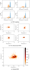 |
Fig. A.1 Constructing PDFs for individual galaxies. Top four panels: analytic PDFs assumed for parameter 1 (blue) and parameter 2 (orange). We then created 100 random samples drawn from each distribution, and the results for each parameter are shown as the shaded histograms of the corresponding colours. Middle panels: two-dimensional PDFs for each hypothetical“galaxy”, derived by assuming that the samples shown in the top panels for each parameter are independent. Bottom panel: stack of the individual two-dimensional PDFs for the four model galaxies and the two indicative parameters shown in the upper panels. The colour bar indicates the number of model galaxies that we expect in each bin; the total obtained by summing all of the pixel values equals the total number of galaxies in the stack. Clearly, individual pixels can take non-integer values since we have sampled each galaxy 100 times. |
To study the relation between the two parameters for the full population (in this case, the hypothetical population of four galaxies, though in Sect. 3.1 we used around 120 000 galaxies), we can then stack the PDFs by summing up the values of the individual two-dimensional PDFs in each bin. The results for our hypothetical data set are shown in Fig. A.1c: with increasingly large numbers of galaxies, these PDFs become increasingly smooth, to the point that (as in Fig. 5) the distribution appears continuous despite the individual galaxies being sampled only 100 times. Each pixel in the stack shows how many galaxies we would expect to find in that bin; since we have sampled each galaxy multiple times and re-normalised (to retain the correct total number of galaxies), these need not be integers, as shown in Fig. A.1c.
Appendix B Studying SFR-L150 with a 150 MHz-selected sample
Many previous works have investigated the SFR – radio luminosity relation using a sample identified at radio frequencies (e.g. Bell 2003; Murphy et al. 2011; Brown et al. 2017; Calistro Rivera et al. 2017; Wang et al. 2019). To see the possible impact of this on our results for SFR-L150 MHz, we repeatedour analysis, but instead included only those sources that are detected at 150 MHz with ≥ 5σ significance.
Figure B.1 reveals that making this kind of selection gives results that are biased to higher L150 at a given SFR (relative to both our IRAC-selected sample shown in Fig. 8 and to the best-fit relation from G18, which is shown as the solid orange line). Dividing such a sample into four redshift bins also reveals an apparent evolution in SFR-L150 MHz – in the sense of an apparent increase in L150 MHz at a given SFRat higher redshift – which is not recovered when the full IRAC-selected sample is considered.
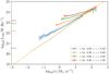 |
Fig. B.1 SFR-L150 MHz plane, as inFig. 5. The coloured lines with error bars indicate the SFR-L150 MHz relation recovered in each of the four redshift bins detailed in the legend – identical to those used in Fig. 8, and which are also reproduced here as the circles – but including only those sources with ≥ 5σ 150 MHzdetections. Also overlaid is the best-fit relation from G18; the horizontal bars adjacent to the left-hand vertical axis indicate the luminosity corresponding to 60 μJy at the lower bound of each redshift bin. |
We conclude that great care is required when interpreting the results of this type of study, based on radio-frequency selected samples, even when using the most sensitive radio data in existence, such as the data used in this work from the LoTSS ELAIS-N1 deep field.
Appendix C Supporting simulations
In order to test that our method of determining the median-likelihood SFR is able to recover the true SFR-L150 MHz relation, we conducted a set of simulations, each based on sampling 120 000 model galaxies with a range of SFRs, stellar masses, and redshifts from our real data. We assigned each galaxy a true L150 MHz value using an arbitrary mass-dependent SFR-L150 MHz relation following Eq. (2), and we simulated Gaussian scatter about that relation assuming a standard width (in dex). Using Eq. (2), we were also able to simulate a stellar-mass independent SFR-L150 MHz relation by setting γ = 0.
We then generated a set of mock observed data by converting the noiseless values of L150 MHz to true flux densities at 150 MHz, before adding on Gaussian noise using a random number generator multiplied by the flux density uncertainty measured for the real sources in our LoTSS catalogue. We also simulated measuring the SFRs (and stellar masses if required) by resampling the true values to give model-observed values with uncertainties that were sampled in the same way as our real MAGPHYS results. Our simulations account for AGN contamination by randomly assigning galaxies an excess radio luminosity drawn from a log-normal distribution with a mean of 23.86 and a standard deviation of 0.91, based on the mean and standard deviation of the L150 MHz of the flagged AGN in the Best et al. (in prep.) sample. The probability that a model galaxy is given such an excess luminosity is based on a mass-dependent probability using the luminosity-averaged results from Sabater et al. (2019), which are shown in Table C.1.
Probability that a galaxy of a given stellar mass is assigned a radio luminosity excess in our simulations, based on the luminosity-averaged results from Sabater et al. (2019).
We then attempted to recover the known relation using the method discussed in Sect. 3.1. Figure C.1 shows an example visualisation of the two-dimensional PDF obtained from one of the simulations, assuming an SFR-L150 MHz relation of the mass-independent form given in Eq. (1) with β = 1.01, log10L1 = 22.15 (shown as the dashed pink line), and with scatter σL = 0.25 dex. The thick red line shows the median-likelihood estimate of the L150 MHz in bins of SFR, while the purple line shows the best fit to the data over the range − 1< ψ < 1, the same range used for the real data. It is clear that, just as in the real data, the median-likelihood estimate (thick red line) appears to be offset to lower SFRs than the apparent peak in the PDF, and it suggests that our explanation for this effect in Sect. 3.1 is plausible.
To better quantify the level of agreement between the input and output parameters in plausible realistic circumstances, we conducted 1000 Monte Carlo simulations of 120 000 model sources. We assumed a range of true values, 0.5 ≤ β ≤ 1.0, 21.5≤ log10LC ≤ 22.5, and 0.30< γ < 0.60, in ten equal steps each, and a fixed scatter of σL = 0.25.
We conducted the simulations twice: once simulating the recovery of the true input parameters for the mass-independent SFR-L150 MHz (results displayed in Fig. C.2) and once simulating the recovery of the mass-dependent version (results displayed inFig. C.3). In Fig. C.2, the left-hand panel shows the recovery of β, while the right-hand panel shows how well L1 is recovered.The 1:1 relation is indicated by the dotted line, while the best-fit relation between the input and the “observed” values is shown as the dashed grey line. The best fit relationships between the input and observed values are:

where the superscripts indicate the observed and true (i.e. model input) parameters. For the best-fit values quoted in Sect. 3.1, the difference in the parameters is small: Δβ ≡ βtrue − βobs = 0.016 and  , with scatter about the best-fit relation of σβ = 0.006 and
 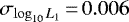 ; we quoted these systematic offsets and propagated the uncertainties on the values quoted in Sect. 3.1.
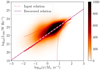 |
Fig. C.1 Heatmap showing the stacked two-dimensional PDF derived based on 120 000 galaxies with a redshift distribution sampled from our real data set and accounting for the uncertainties in both SFR and L150 MHz as in Fig. 5. The median-likelihood estimate of the SFR-L150 MHz relation is shown as the thick red line, while the recovered relation (in purple) is very close to the true SFR-L150 MHz relation (dashed pink line). The colour bar to the right shows the effective number of galaxies in each bin. |
Similarly for the three-dimensional simulations, using ten bins of β, log10LC, and γ, the best-fit relations are:
 (C.3)
(C.3)
 (C.4)
(C.4)
 (C.5)
(C.5)
For the best-fit values quoted in Sect. 3.4, the difference in the quoted parameters is Δβ ≡ βtrue − βobs = 0.051,  , and Δγ ≡ γtrue − γobs = − 0.057. The mean scatter about each best-fit relation dominates the uncertainties on these corrections, and the values are σβ = 0.011,
 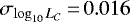 , and σγ = 0.037.
C.1 Flux density limit or mass dependence?
Finally, we performed two further tests to see whether the possible redshift-dependent upturn to higher L150 MHz at lower SFRs shown in Fig. 8 is real or an artefact of the finite S/N available in the 150 MHz data set. First, we created a simulation identical to the ones in the previous section, with an input SFR-L150 MHz relation that is independent of mass and repeated the analysis from Sect. 3.3 to see how well it was recovered. The left-hand panel of Fig. C.4 shows the results: while there is a slight bias towards a flatter SFR-L150 MHz relation (as discussed in Appendix C), there is no evidence of an upturn, including below the approximate flux density limits indicated for each redshift bin by the horizontal error bars adjacent to the left vertical axis.
In the right-hand panel of Fig. C.4, we show the results of repeating an identicalanalysis using a second simulation, which includes a mass-dependent SFR-L150 MHz relation of the form given in Eq. (2). The upturn to higher L150 MHz towards lower SFRs is now clear, underlining our view that this effect – if real – is consistent with being a consequence of the mass dependence in the SFR-L150 MHz relation.
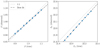 |
Fig. C.2 Simulations showing the observed values of β and L1 obtained using the method described in Sect. 3.1 as a function of the known input values, assuming a fixed width of σL = 0.25 and mass-dependent AGN contamination following Sabater et al. (2019). The best-fit relations between the two sets of values – shown as the dashed grey line – are given in the text. The 1:1 line is shown as the dotted line. |
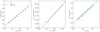 |
Fig. C.3 Simulations showing the observed values of β and L1 obtained using the method described in Sect. 3.1 as a function of the known input values, assuming a fixed width of σL = 0.25 and AGN contamination following Sabater et al. (2019). The best-fit relations between the two sets of values are shown as the dashed grey lines, and they are parameterised as in the text. The dotted line in each panel shows the 1:1 relation. |
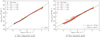 |
Fig. C.4 Simulations of possible redshift evolution in the SFR-L150 MHz relation using: (a) a mass-independent input relation of the form given in Eq. (1), and (b) a mass-dependent input relation of the form given in Eq. (2). The method used to obtain these figures is identical, and only the mass-dependent simulation reveals an upturn in L150 MHz at lower SFRs, as seen for the real data set analysed in Fig. 8 (see that caption for further details). |
References
- Aihara, H., Arimoto, N., Armstrong, R., et al. 2018, PASJ, 70, S4 [NASA ADS] [Google Scholar]
- Antonucci, R. 1993, ARA&A, 31, 473 [Google Scholar]
- Appleton, P. N., Fadda, D. T., Marleau, F. R., et al. 2004, ApJS, 154, 147 [NASA ADS] [CrossRef] [Google Scholar]
- Becker, R. H., White, R. L., & Helfand, D. J. 1995, ApJ, 450, 559 [NASA ADS] [CrossRef] [Google Scholar]
- Bell, E. F. 2003, ApJ, 586, 794 [Google Scholar]
- Berta, S., Lutz, D., Santini, P., et al. 2013, A&A, 551, A100 [NASA ADS] [CrossRef] [EDP Sciences] [Google Scholar]
- Best, P. N., & Heckman, T. M. 2012, MNRAS, 421, 1569 [NASA ADS] [CrossRef] [Google Scholar]
- Bonato, M., Negrello, M., Mancuso, C., et al. 2017, MNRAS, 469, 1912 [Google Scholar]
- Bourne, N., Dunne, L., Ivison, R. J., et al. 2011, MNRAS, 410, 1155 [NASA ADS] [CrossRef] [Google Scholar]
- Brinchmann, J., Charlot, S., White, S. D. M., et al. 2004, MNRAS, 351, 1151 [NASA ADS] [CrossRef] [Google Scholar]
- Brown, M. J. I., Moustakas, J., Kennicutt, R. C., et al. 2017, ApJ, 847, 136 [NASA ADS] [CrossRef] [Google Scholar]
- Bruzual, G., & Charlot, S. 2003, MNRAS, 344, 1000 [NASA ADS] [CrossRef] [Google Scholar]
- Burgarella, D., Buat, V., & Iglesias-Páramo, J. 2005, MNRAS, 360, 1413 [Google Scholar]
- Calistro Rivera, G., Lusso, E., Hennawi, J. F., & Hogg, D. W. 2016, ApJ, 833, 98 [NASA ADS] [CrossRef] [Google Scholar]
- Calistro Rivera, G., Williams, W. L., Hardcastle, M. J., et al. 2017, MNRAS, 469, 3468 [NASA ADS] [CrossRef] [Google Scholar]
- Carilli, C. L., & Rawlings, S. 2004, New Astron. Rev., 48, 979 [Google Scholar]
- Carnall, A. C., McLure, R. J., Dunlop, J. S., & Davé, R. 2018, MNRAS, 480, 4379 [NASA ADS] [CrossRef] [Google Scholar]
- Chabrier, G. 2003, PASP, 115, 763 [Google Scholar]
- Chambers, K. C., Magnier, E. A., Metcalfe, N., et al. 2016, ArXiv e-prints [arXiv:1612.05560] [Google Scholar]
- Charlot, S., & Fall, S. M. 2000, ApJ, 539, 718 [Google Scholar]
- Chi, X., & Wolfendale, A. W. 1990, MNRAS, 245, 101 [Google Scholar]
- Condon, J. J. 1992, ARA&A, 30, 575 [NASA ADS] [CrossRef] [MathSciNet] [Google Scholar]
- Cram, L., Hopkins, A., Mobasher, B., & Rowan-Robinson, M. 1998, ApJ, 507, 155 [NASA ADS] [CrossRef] [Google Scholar]
- da Cunha, E., Charlot, S., & Elbaz, D. 2008, MNRAS, 388, 1595 [Google Scholar]
- Dalton, G. 2016, ASP Conf. Ser., 507, 97 [Google Scholar]
- Davies, L. J. M., Huynh, M. T., Hopkins, A. M., et al. 2017, MNRAS, 466, 2312 [Google Scholar]
- De Gasperin, F., Williams, W. L., Best, P., et al. 2021, A&A, in press, https://doi.org/10.1051/0004-6361/202140316 [Google Scholar]
- de Jong, T., Klein, U., Wielebinski, R., & Wunderlich, E. 1985, A&A, 147, L6 [NASA ADS] [Google Scholar]
- Delhaize, J., Smolčić, V., Delvecchio, I., et al. 2017, A&A, 602, A4 [NASA ADS] [CrossRef] [EDP Sciences] [Google Scholar]
- Dewdney, P. E., Hall, P. J., Schilizzi, R. T., & Lazio, T. J. L. W. 2009, IEEE Proc., 97, 1482 [Google Scholar]
- Donley, J. L., Koekemoer, A. M., Brusa, M., et al. 2012, ApJ, 748, 142 [Google Scholar]
- Driver, S. P., Hill, D. T., Kelvin, L. S., et al. 2011, MNRAS, 413, 971 [Google Scholar]
- Dudzevičiūtė, U., Smail, I., Swinbank, A. M., et al. 2020, MNRAS, 494, 3828 [Google Scholar]
- Duncan, K. J., Sabater, J., Röttgering, H. J. A., et al. 2019, A&A, 622, A3 [NASA ADS] [CrossRef] [EDP Sciences] [Google Scholar]
- Duncan, K. J., Shivaei, I., Shapley, A. E., et al. 2020, Phys. Rev. D, 91, 043510 [Google Scholar]
- Duncan, K., Kondapally, R., Brown, M., et al. 2021, A&A, 648, A4 (LoTSS SI) [EDP Sciences] [Google Scholar]
- Flesch, E. W. 2019, ArXiv e-prints [arXiv:1912.05614] [Google Scholar]
- Foreman-Mackey, D., Hogg, D. W., Lang, D., & Goodman, J. 2013, PASP, 125, 306 [Google Scholar]
- Garn, T., Green, D. A., Riley, J. M., & Alexander, P. 2009, MNRAS, 397, 1101 [NASA ADS] [CrossRef] [Google Scholar]
- Gott, J. R., I., Vogeley, M. S., Podariu, S., & Ratra, B. 2001, ApJ, 549, 1 [NASA ADS] [CrossRef] [Google Scholar]
- Gürkan, G., Hardcastle, M. J., Smith, D. J. B., et al. 2018, MNRAS, 475, 3010 [NASA ADS] [CrossRef] [Google Scholar]
- Haarsma, D. B., Partridge, R. B., Windhorst, R. A., & Richards, E. A. 2000, ApJ, 544, 641 [NASA ADS] [CrossRef] [Google Scholar]
- Hardcastle, M. J., Evans, D. A., & Croston, J. H. 2007, MNRAS, 376, 1849 [NASA ADS] [CrossRef] [Google Scholar]
- Hardcastle, M. J., Gürkan, G., van Weeren, R. J., et al. 2016, MNRAS, 462, 1910 [NASA ADS] [CrossRef] [Google Scholar]
- Hardcastle, M. J., Croston, J. H., Shimwell, T. W., et al. 2019a, MNRAS, 488, 3416 [NASA ADS] [CrossRef] [Google Scholar]
- Hardcastle, M. J., Williams, W. L., Best, P. N., et al. 2019b, A&A, 622, A12 [NASA ADS] [CrossRef] [EDP Sciences] [Google Scholar]
- Hayward, C. C., & Smith, D. J. B. 2015, MNRAS, 446, 1512 [NASA ADS] [CrossRef] [Google Scholar]
- Helou, G., Soifer, B. T., & Rowan-Robinson, M. 1985, ApJ, 298, L7 [Google Scholar]
- Hodge, J. A., Becker, R. H., White, R. L., & de Vries, W. H. 2008, AJ, 136, 1097 [Google Scholar]
- Hopkins, A. M., Miller, C. J., Nichol, R. C., et al. 2003, ApJ, 599, 971 [NASA ADS] [CrossRef] [Google Scholar]
- Hurley, P. D., Oliver, S., Betancourt, M., et al. 2017, MNRAS, 464, 885 [NASA ADS] [CrossRef] [Google Scholar]
- Intema, H. T., Jagannathan, P., Mooley, K. P., & Frail, D. A. 2017, A&A, 598, A78 [NASA ADS] [CrossRef] [EDP Sciences] [Google Scholar]
- Ivison, R. J., Alexander, D. M., Biggs, A. D., et al. 2010a, MNRAS, 402, 245 [NASA ADS] [CrossRef] [Google Scholar]
- Ivison, R. J., Magnelli, B., Ibar, E., et al. 2010b, A&A, 518, L31 [NASA ADS] [CrossRef] [EDP Sciences] [Google Scholar]
- Jarvis, M. J., Smith, D. J. B., Bonfield, D. G., et al. 2010, MNRAS, 409, 92 [NASA ADS] [CrossRef] [Google Scholar]
- Johnston, R., Vaccari, M., Jarvis, M., et al. 2015, MNRAS, 453, 2540 [NASA ADS] [CrossRef] [Google Scholar]
- Karim, A., Schinnerer, E., Martínez-Sansigre, A., et al. 2011, ApJ, 730, 61 [NASA ADS] [CrossRef] [Google Scholar]
- Kellermann, K. I., & Owen, F. N. 1988, Galactic and Extragalactic Radio Astronomy (Berlin: Springer), 563 [Google Scholar]
- Kennicutt, R. C., J. 1998, ARA&A, 36, 189 [Google Scholar]
- Kennicutt, R. C., & Evans, N. J. 2012, ARA&A, 50, 531 [NASA ADS] [CrossRef] [Google Scholar]
- Kennicutt, R. C., J., Hao, C.-N., Calzetti, D., et al. 2009, ApJ, 703, 1672 [NASA ADS] [CrossRef] [Google Scholar]
- Kondapally, R., Best, P., Hardcastle, M., et al. 2021, A&A, 648, A3 (LoTSS SI) [EDP Sciences] [Google Scholar]
- Lacki, B. C., & Thompson, T. A. 2010, ApJ, 717, 196 [NASA ADS] [CrossRef] [Google Scholar]
- Lacki, B. C., Thompson, T. A., & Quataert, E. 2010, ApJ, 717, 1 [NASA ADS] [CrossRef] [Google Scholar]
- Lacy, M., Storrie-Lombardi, L. J., Sajina, A., et al. 2004, ApJS, 154, 166 [Google Scholar]
- Lawrence, A., Warren, S. J., Almaini, O., et al. 2007, MNRAS, 379, 1599 [NASA ADS] [CrossRef] [MathSciNet] [Google Scholar]
- Leslie, S., Schinnerer, E., Liu, D., et al. 2020, ApJ, 899, 58 [Google Scholar]
- Lisenfeld, U., Voelk, H. J., & Xu, C. 1996, A&A, 306, 677 [Google Scholar]
- Lofthouse, E. K., Kaviraj, S., Smith, D. J. B., & Hardcastle, M. J. 2018, MNRAS, 479, 807 [Google Scholar]
- Lonsdale, C. J., Smith, H. E., Rowan-Robinson, M., et al. 2003, PASP, 115, 897 [NASA ADS] [CrossRef] [Google Scholar]
- Macfarlane, C., Best, P. N., Sabater, J., & Gürkan, G. 2020, MNRAS, submitted [Google Scholar]
- Madau, P., & Dickinson, M. 2014, ARA&A, 52, 415 [NASA ADS] [CrossRef] [Google Scholar]
- Magnelli, B., Ivison, R. J., Lutz, D., et al. 2015, A&A, 573, A45 [NASA ADS] [CrossRef] [EDP Sciences] [Google Scholar]
- Mahatma, V. H., Hardcastle, M. J., Williams, W. L., et al. 2019, A&A, 622, A13 [NASA ADS] [CrossRef] [EDP Sciences] [Google Scholar]
- Malefahlo, E., Santos, M. G., Jarvis, M. J., White, S. V., & Zwart, J. T. L. 2020, MNRAS, 492, 5297 [Google Scholar]
- Martínez-Sansigre, A., Rawlings, S., Lacy, M., et al. 2005, Nature, 436, 666 [NASA ADS] [CrossRef] [Google Scholar]
- Mauch, T., Klöckner, H.-R., Rawlings, S., et al. 2013, MNRAS, 435, 650 [NASA ADS] [CrossRef] [Google Scholar]
- Mauduit, J. C., Lacy, M., Farrah, D., et al. 2012, PASP, 124, 714 [NASA ADS] [CrossRef] [Google Scholar]
- McAlpine, K., Smith, D. J. B., Jarvis, M. J., Bonfield, D. G., & Fleuren, S. 2012, MNRAS, 423, 132 [NASA ADS] [CrossRef] [Google Scholar]
- Molnár, D. C., Sargent, M. T., Delhaize, J., et al. 2018, MNRAS, 475, 827 [NASA ADS] [CrossRef] [Google Scholar]
- Murphy, E. J. 2009, ApJ, 706, 482 [NASA ADS] [CrossRef] [Google Scholar]
- Murphy, E. J., Helou, G., Kenney, J. D. P., Armus, L., & Braun, R. 2008, ApJ, 678, 828 [NASA ADS] [CrossRef] [Google Scholar]
- Murphy, E. J., Condon, J. J., Schinnerer, E., et al. 2011, ApJ, 737, 67 [NASA ADS] [CrossRef] [Google Scholar]
- Muzzin, A., Wilson, G., Yee, H. K. C., et al. 2009, ApJ, 698, 1934 [NASA ADS] [CrossRef] [Google Scholar]
- Nisbet, D. M. 2018, PhD thesis, University of Edinburgh, UK [Google Scholar]
- Noeske, K. G., Weiner, B. J., Faber, S. M., et al. 2007, ApJ, 660, L43 [Google Scholar]
- Novak, M., Smolčić, V., Delhaize, J., et al. 2017, A&A, 602, A5 [NASA ADS] [CrossRef] [EDP Sciences] [Google Scholar]
- Oliver, S. J., Bock, J., Altieri, B., et al. 2012, MNRAS, 424, 1614 [Google Scholar]
- Pannella, M., Carilli, C. L., Daddi, E., et al. 2009, ApJ, 698, L116 [Google Scholar]
- Pannella, M., Elbaz, D., Daddi, E., et al. 2015, ApJ, 807, 141 [NASA ADS] [CrossRef] [Google Scholar]
- Pearson, W. J., Wang, L., van der Tak, F. F. S., et al. 2017, A&A, 603, A102 [NASA ADS] [CrossRef] [EDP Sciences] [Google Scholar]
- Pozzetti, L., Bolzonella, M., Zucca, E., et al. 2010, A&A, 523, A13 [NASA ADS] [CrossRef] [EDP Sciences] [Google Scholar]
- Prescott, M., Mauch, T., Jarvis, M. J., et al. 2016, MNRAS, 457, 730 [Google Scholar]
- Read, S. C. 2019, PhD thesis, University of Hertfordshire, UK [Google Scholar]
- Read, S. C., Smith, D. J. B., Gürkan, G., et al. 2018, MNRAS, 480, 5625 [NASA ADS] [CrossRef] [Google Scholar]
- Read, S. C., Smith, D. J. B., Jarvis, M. J., & Gürkan, G. 2020, MNRAS, 492, 3940 [Google Scholar]
- Retana-Montenegro, E., Röttgering, H. J. A., Shimwell, T. W., et al. 2018, A&A, 620, A74 [NASA ADS] [CrossRef] [EDP Sciences] [Google Scholar]
- Röttgering, H., Afonso, J., Barthel, P., et al. 2011, JApA, 32, 557 [NASA ADS] [CrossRef] [Google Scholar]
- Sabater, J., Best, P. N., Hardcastle, M. J., et al. 2019, A&A, 622, A17 [NASA ADS] [CrossRef] [EDP Sciences] [Google Scholar]
- Sabater, J., Best, P., Tasse, C., et al. 2021, A&A, 648, A2 (LoTSS SI) [EDP Sciences] [Google Scholar]
- Sadler, E. M., Jackson, C. A., Cannon, R. D., et al. 2002, MNRAS, 329, 227 [NASA ADS] [CrossRef] [Google Scholar]
- Sargent, M. T., Schinnerer, E., Murphy, E., et al. 2010, ApJ, 714, L190 [NASA ADS] [CrossRef] [Google Scholar]
- Schreiber, C., Pannella, M., Elbaz, D., et al. 2015, A&A, 575, A74 [NASA ADS] [CrossRef] [EDP Sciences] [Google Scholar]
- Shimwell, T. W., Röttgering, H. J. A., Best, P. N., et al. 2017, A&A, 598, A104 [NASA ADS] [CrossRef] [EDP Sciences] [Google Scholar]
- Shimwell, T. W., Tasse, C., Hardcastle, M. J., et al. 2019, A&A, 622, A1 [NASA ADS] [CrossRef] [EDP Sciences] [Google Scholar]
- Shirley, R., Roehlly, Y., Hurley, P. D., et al. 2019, MNRAS, 490, 634 [CrossRef] [Google Scholar]
- Smith, D. J. B., & Hayward, C. C. 2018, MNRAS, 476, 1705 [CrossRef] [Google Scholar]
- Smith, D. J. B., Dunne, L., Maddox, S. J., et al. 2011, MNRAS, 416, 857 [NASA ADS] [CrossRef] [Google Scholar]
- Smith, D. J. B., Dunne, L., da Cunha, E., et al. 2012, MNRAS, 427, 703 [NASA ADS] [CrossRef] [Google Scholar]
- Smith, D. J. B., Jarvis, M. J., Hardcastle, M. J., et al. 2014, MNRAS, 445, 2232 [NASA ADS] [CrossRef] [Google Scholar]
- Smith, D. J. B., Best, P. N., Duncan, K. J., et al. 2016, SF2A-2016: Proceedings of the Annual meeting of the French Society of Astronomy and Astrophysics, eds. C. Reylé, J. Richard, L. Cambrésy, et al., 271 [Google Scholar]
- Smolčić, V., Novak, M., Bondi, M., et al. 2017, A&A, 602, A1 [NASA ADS] [CrossRef] [EDP Sciences] [Google Scholar]
- Sudoh, T., Linden, T., & Beacom, J. F. 2020, ArXiv e-prints [arXiv:2005.08982] [Google Scholar]
- Sutherland, W., & Saunders, W. 1992, MNRAS, 259, 413 [NASA ADS] [CrossRef] [Google Scholar]
- Tabatabaei, F. S., Schinnerer, E., Krause, M., et al. 2017, ApJ, 836, 185 [Google Scholar]
- Tacchella, S., Dekel, A., Carollo, C. M., et al. 2016, MNRAS, 457, 2790 [NASA ADS] [CrossRef] [Google Scholar]
- Tasse, C., Shimwell, T., Hardcastle, M., et al. 2021, A&A, 648, A1 (LoTSS SI) [EDP Sciences] [Google Scholar]
- Upjohn, J. E., Brown, M. J. I., Hopkins, A. M., & Bonne, N. J. 2019, PASA, 36, e012 [Google Scholar]
- van der Kruit,P. C. 1971, A&A, 15, 110 [Google Scholar]
- van Haarlem, M. P., Wise, M. W., Gunst, A. W., et al. 2013, A&A, 556, A2 [NASA ADS] [CrossRef] [EDP Sciences] [Google Scholar]
- Wang, L., Rowan-Robinson, M., Norberg, P., Heinis, S., & Han, J. 2014, MNRAS, 442, 2739 [NASA ADS] [CrossRef] [Google Scholar]
- Wang, L., Gao, F., Duncan, K. J., et al. 2019, A&A, 631, A109 [CrossRef] [EDP Sciences] [Google Scholar]
- Williams, W. L., Hardcastle, M. J., Best, P. N., et al. 2019, A&A, 622, A2 [NASA ADS] [CrossRef] [EDP Sciences] [Google Scholar]
- Wilson, G., Muzzin, A., Yee, H. K. C., et al. 2009, ApJ, 698, 1943 [NASA ADS] [CrossRef] [Google Scholar]
- York, D. G., Adelman, J., Anderson, J. E., J., et al. 2000, AJ, 120, 1579 [CrossRef] [Google Scholar]
- Yun, M. S., Reddy, N. A., & Condon, J. J. 2001, ApJ, 554, 803 [NASA ADS] [CrossRef] [Google Scholar]
- Zwart, J. T. L., Jarvis, M. J., Deane, R. P., et al. 2014, MNRAS, 439, 1459 [NASA ADS] [CrossRef] [Google Scholar]
- Zwart, J. T. L., Santos, M., & Jarvis, M. J. 2015, MNRAS, 453, 1740 [NASA ADS] [CrossRef] [Google Scholar]
We note that the slope of 0.75 ± 0.03 quoted by Davies et al. (2017) uses the inverse definition of the SFR – radio luminosity relation, which is why the quoted value is lower than unity.
As noted in Kondapally et al. (2021), in the ELAIS-N1 field, the necessary flags to apply are flag_clean=1 & flag_overlap=7.
The scatter is measured in terms of the normalised median absolute deviation, which is defined as σNMAD = 1.48 × median(|Δz|∕(1 + zspec)), while outliers are defined as those sources where |Δz|∕(1 + zspec) > 0.15.
We repeated all of the following analysis both with and without including these sources in the analysis, and the results do not show significant variation.
This is not unreasonable given the immense SED-fitting effort required to replicate them for the full IRAC-selected sample.
Appendix A describes an illustrative example of this method, along with more of the intermediate steps for the interested reader.
We can consider, for example, that the ± 2σ confidence interval in log values for a 3σ source with a true luminosity of 1024 W Hz−1 is 23.52 < log10(L150 MHz∕W Hz−1) < 24.22. The range is more than twice as large on the negative side as on positive side.
All Tables
Percentage of the area covered in this study by each set of ancillary data used for the SED fitting, along with the mean percentage of sources detected at ≥ 3σ in the most sensitive band of each data set.
Percentage of sources in our parent sample with measured photometry (middle column) and a ≥ 3σ detection in at least N bands.
Probability that a galaxy of a given stellar mass is assigned a radio luminosity excess in our simulations, based on the luminosity-averaged results from Sabater et al. (2019).
All Figures
|
Fig. 1 Filter curves of the assembled multi-wavelength data set (coloured lines), overlaid with a galaxy template from Smith et al. (2012). The SED has been normalised to have a peak flux of 1, and it is shown both at z = 0 (in grey) andwith the wavelength axis shifted to z = 1 (in silver) to give the reader an impression of how the excellent multi-wavelength coverage in ELAIS-N1 samples a galaxy’s SED. |
| In the text | |
|
Fig. 2 Histograms (clockwise from the top-left) showing the SFR (ψ), stellar mass, 150 MHz S/N, and redshift distributions for the 118 517 galaxies in our 3.6 μm-selected z < 1 sample after applying the cuts discussed in Sect. 2. The overlaid orange histograms show the corresponding distributions for the subset of the sample that is detected to ≥ 3σ at 150 MHz. |
| In the text | |
|
Fig. 3 Heatmaps showing the variation in median-likelihood stellar mass in M⊙ (top) and SFR (ψ) in units of M⊙ yr−1 (bottom) as a function of redshift in our IRAC-selected sample. The redshift axis is common to both plots, and the number of galaxies in each bin is indicated by the colour scales to the right. Upper panel: the dashed blue line indicates the 95% mass completeness limit as a function of redshift, derived using the method from Pozzetti et al. (2010). |
| In the text | |
|
Fig. 4 SFR-L150 MHz plane populated by the 25 777 sources with ≥3σ detections in the 150 MHz data, with the colour bar to the right indicating the bin occupancy. The best-fit relations from G18 are overlaid for comparison; the mass-independent relation is shown in orange, while the broken power-law relation evaluated at 1010 M⊙ is shown as the dashed blue line. |
| In the text | |
|
Fig. 5 Stacked heatmap showing the two-dimensional PDF for SFR and L150 MHz for all 118 517 galaxies in our sample, including the uncertainties on the SFR (derived based on the percentiles of the MAGPHYS SFR PDF) and on L150 MHz (using the pixel flux densities and rms values at the redshift in the Duncan et al. 2021 catalogue). The “effective” number of galaxies in each bin – we recall that each galaxy is sampled 100 times (with each sample representing 0.01 galaxies) and can therefore contribute to multiple pixels in the stack – is indicated by the colour bar to the right. The best-fit SFR-L150 MHz relationship from G18 is overlaid as the solid orange line, along with the broken power-law G18 relation (which we have evaluated at a canonical stellar mass of 1010 M⊙, and which is shown as the dashed blue line) along with (in red) the 16th, 50th, and 84th percentiles of the L150 MHz distribution at each SFR. |
| In the text | |
|
Fig. 6 Histogram with logarithmic ordinates, showing the true observed flux density distribution (in red) overlaid on individual Monte Carlo realisations (shown in grey with transparency, such that lighter shading indicates the range of outputs) based on assuming the best-fit SFR-L150 MHz relation from Sect. 3.1 with the full range of intrinsic scatter 0.0 < σL < 0.5. |
| In the text | |
|
Fig. 7 Variation in median-likelihood estimates of σL as a function of the central value of each SFR bin. The error bars in the vertical direction are derived from the 16th and 84th percentiles of the PDF, while in the horizontal direction the error bars indicate the bin width. Also overlaid are red circles, indicating the Bayesian estimates of scatter from the PDF, calculated according to the product of Σ σLP (σL). |
| In the text | |
|
Fig. 8 Median-likelihood estimates of the SFR-L150 MHz relation for the wholesample (red circles) and in four redshift bins (0.05 < z < 0.30, 0.30 < z < 0.60, 0.60 < z < 0.80, and 0.80 < z < 1.00 are shown as the blue, orange, green, and red crosses, respectively). Error bars on the median L150 MHz are calculatedusing the median statistics method from Gott et al. (2001). Also overlaid are the SFR-L150 MHz relationships from Bell (2003, dot-dashed purple line) and Murphy et al. (2011, dashed cyan line), converted to 150 MHz assuming a canonical spectral index α = 0.7, and the 150 MHz relations from G18 (mass-independent shown as the solid orange line, broken power law evaluated at 1010 M⊙ as the dashed purple line) and Wang et al. (2019) (shown as the dotted blue line). The literature calibrations have been converted toour adopted IMF from Chabrier (2003) using the factors recommended in Madau & Dickinson (2014). The horizontal coloured lines immediately to the right of the left-hand vertical axis indicate the luminosity corresponding to the 60 μJy at the lower redshift bound of each bin, as indicated by the colour (see text for details). |
| In the text | |
|
Fig. 9 Variation in σL for galaxies with 0.5 < log10ψ < 1.5, 10 < log10(M∕M⊙) < 11 as a function of redshift – with error bars derived from the 16th and 84th percentiles of the PDF – and centred on the median-likelihood values. The error bars in the redshift (horizontal) direction indicate the bounds of each redshift bin. |
| In the text | |
|
Fig. 10 L150 MHz dependence with SFR and stellar mass. Left: SFR-L150 MHz relation as a function of stellar mass, indicated by the colour of the line and relative to the colour bar, overlaid on the mass-independent relation from G18 (solid orange line) and our best-fit estimate from Sect. 3.1 (dashed blue line). Each coloured line shows the median-likelihood L150 MHz at a given SFR and stellar mass. Right: relationship between stellar mass and median-likelihood L150 MHz, coloured as a function of SFR with the scale indicated by the bar to the right. |
| In the text | |
|
Fig. 11 Accounting for stellar mass effects in SFR-L150 MHz. Left: SFR-L150 MHz relationship with the mass dependence taken out using Eq. (2) and the best-fit parameters. Stellar mass is indicated by the colour bar to the right. Right: same as the left, but with the relationship between the stellar mass and radio luminosity normalised by the SFR using Eq. (2). |
| In the text | |
|
Fig. A.1 Constructing PDFs for individual galaxies. Top four panels: analytic PDFs assumed for parameter 1 (blue) and parameter 2 (orange). We then created 100 random samples drawn from each distribution, and the results for each parameter are shown as the shaded histograms of the corresponding colours. Middle panels: two-dimensional PDFs for each hypothetical“galaxy”, derived by assuming that the samples shown in the top panels for each parameter are independent. Bottom panel: stack of the individual two-dimensional PDFs for the four model galaxies and the two indicative parameters shown in the upper panels. The colour bar indicates the number of model galaxies that we expect in each bin; the total obtained by summing all of the pixel values equals the total number of galaxies in the stack. Clearly, individual pixels can take non-integer values since we have sampled each galaxy 100 times. |
| In the text | |
|
Fig. B.1 SFR-L150 MHz plane, as inFig. 5. The coloured lines with error bars indicate the SFR-L150 MHz relation recovered in each of the four redshift bins detailed in the legend – identical to those used in Fig. 8, and which are also reproduced here as the circles – but including only those sources with ≥ 5σ 150 MHzdetections. Also overlaid is the best-fit relation from G18; the horizontal bars adjacent to the left-hand vertical axis indicate the luminosity corresponding to 60 μJy at the lower bound of each redshift bin. |
| In the text | |
|
Fig. C.1 Heatmap showing the stacked two-dimensional PDF derived based on 120 000 galaxies with a redshift distribution sampled from our real data set and accounting for the uncertainties in both SFR and L150 MHz as in Fig. 5. The median-likelihood estimate of the SFR-L150 MHz relation is shown as the thick red line, while the recovered relation (in purple) is very close to the true SFR-L150 MHz relation (dashed pink line). The colour bar to the right shows the effective number of galaxies in each bin. |
| In the text | |
|
Fig. C.2 Simulations showing the observed values of β and L1 obtained using the method described in Sect. 3.1 as a function of the known input values, assuming a fixed width of σL = 0.25 and mass-dependent AGN contamination following Sabater et al. (2019). The best-fit relations between the two sets of values – shown as the dashed grey line – are given in the text. The 1:1 line is shown as the dotted line. |
| In the text | |
|
Fig. C.3 Simulations showing the observed values of β and L1 obtained using the method described in Sect. 3.1 as a function of the known input values, assuming a fixed width of σL = 0.25 and AGN contamination following Sabater et al. (2019). The best-fit relations between the two sets of values are shown as the dashed grey lines, and they are parameterised as in the text. The dotted line in each panel shows the 1:1 relation. |
| In the text | |
|
Fig. C.4 Simulations of possible redshift evolution in the SFR-L150 MHz relation using: (a) a mass-independent input relation of the form given in Eq. (1), and (b) a mass-dependent input relation of the form given in Eq. (2). The method used to obtain these figures is identical, and only the mass-dependent simulation reveals an upturn in L150 MHz at lower SFRs, as seen for the real data set analysed in Fig. 8 (see that caption for further details). |
| In the text | |
Current usage metrics show cumulative count of Article Views (full-text article views including HTML views, PDF and ePub downloads, according to the available data) and Abstracts Views on Vision4Press platform.
Data correspond to usage on the plateform after 2015. The current usage metrics is available 48-96 hours after online publication and is updated daily on week days.
Initial download of the metrics may take a while.