| Issue |
A&A
Volume 643, November 2020
|
|
|---|---|---|
| Article Number | A177 | |
| Number of page(s) | 25 | |
| Section | Cosmology (including clusters of galaxies) | |
| DOI | https://doi.org/10.1051/0004-6361/202039083 | |
| Published online | 20 November 2020 | |
The search for galaxy cluster members with deep learning of panchromatic HST imaging and extensive spectroscopy⋆
1
Department of Physics and Earth Science of the University of Ferrara, Via Saragat 1, 44122 Ferrara, Italy
e-mail: gius.angora@gmail.com
2
INAF – Astronomical Observatory of Bologna, via Gobetti 93/3, 40129 Bologna, Italy
3
INAF – Astronomical Observatory of Capodimonte, Salita Moiariello 16, 80131 Napoli, Italy
4
Department of Physics of the University of Milano, via Celoria 16, 20133 Milano, Italy
5
Dark Cosmology Centre, Niels Bohr Institute, University of Copenhagen, Lyngbyvej 2, 2100 Copenhagen, Denmark
6
INAF – IASF Milano, Via A. Corti 12, 20133 Milano, Italy
7
Kapteyn Astronomical Institute, University of Groningen, Postbus 800, 9700 AV Groningen, The Netherlands
8
INAF – Astronomical Observatory of Trieste, via G. B. Tiepolo 11, 34131 Trieste, Italy
9
INFN, Sezione di Ferrara, Via Saragat 1, 44122 Ferrara, Italy
Received:
1
August
2020
Accepted:
16
September
2020
Context. The next generation of extensive and data-intensive surveys are bound to produce a vast amount of data, which can be efficiently dealt with using machine-learning and deep-learning methods to explore possible correlations within the multi-dimensional parameter space.
Aims. We explore the classification capabilities of convolution neural networks (CNNs) to identify galaxy cluster members (CLMs) by using Hubble Space Telescope (HST) images of fifteen galaxy clusters at redshift 0.19 ≲ z ≲ 0.60, observed as part of the CLASH and Hubble Frontier Field programmes.
Methods. We used extensive spectroscopic information, based on the CLASH-VLT VIMOS programme combined with MUSE observations, to define the knowledge base. We performed various tests to quantify how well CNNs can identify cluster members on ht basis of imaging information only. Furthermore, we investigated the CNN capability to predict source memberships outside the training coverage, in particular, by identifying CLMs at the faint end of the magnitude distributions.
Results. We find that the CNNs achieve a purity-completeness rate ≳90%, demonstrating stable behaviour across the luminosity and colour of cluster galaxies, along with a remarkable generalisation capability with respect to cluster redshifts. We concluded that if extensive spectroscopic information is available as a training base, the proposed approach is a valid alternative to catalogue-based methods because it has the advantage of avoiding photometric measurements, which are particularly challenging and time-consuming in crowded cluster cores. As a byproduct, we identified 372 photometric cluster members, with mag(F814) < 25, to complete the sample of 812 spectroscopic members in four galaxy clusters RX J2248-4431, MACS J0416-2403, MACS J1206-0847 and MACS J1149+2223.
Conclusions. When this technique is applied to the data that are expected to become available from forthcoming surveys, it will be an efficient tool for a variety of studies requiring CLM selection, such as galaxy number densities, luminosity functions, and lensing mass reconstruction.
Key words: Galaxy: general / galaxies: photometry / galaxies: distances and redshifts / techniques: image processing / methods: data analysis
The spectroscopic training set and the members identified in the four clusters RX J2248-4431, MACS J0416-2403, MACS J1206-0847 and MACS J1149+2223 are only available at the CDS via anonymous ftp to cdsarc.u-strasbg.fr (130.79.128.5) or via http://cdsarc.u-strasbg.fr/viz-bin/cat/J/A+A/643/A177
© ESO 2020
1. Introduction
Over the past decade, the field of astrophysics has been experiencing a true paradigmatic shift, moving rapidly from relatively small data sets to the big data regime. Dedicated survey telescopes, both ground-based and space-borne, are set to routinely produce tens of terabytes of data of unprecedented quality and complexity on a daily basis. These volumes of data can be dealt with through a novel framework, delegating most of the work to automatic tools and by exploiting all advances in high-performance computing, machine learning, data science and visualisation (Brescia et al. 2018). The paradigms of machine learning (ML) and deep learning (DL) paradigms embed the intrinsic data-driven learning capability to explore huge amounts of multi-dimensional data by searching for hidden correlations within the data parameter space.
Here, we explore the application of ML techniques in the context of studies of galaxy clusters, more specifically, to identify cluster members (CLMs) based on imaging data alone. In fact, obtaining a highly complete sample of spectroscopic members is an extremely expensive and time-consuming task, which can be simplified and accelerated thanks to the use of a limited amount of spectroscopic information in training ML methods.
Disentangling CLMs from background and foreground sources is an essential step in the measurement of physical properties of galaxy clusters, measuring, for example, the galaxy luminosity and stellar mass functions (e.g. Annunziatella et al. 2016, 2017), in addition to studies of the cluster mass distribution via strong and weak lensing techniques (e.g. Caminha et al. 2017a, 2019; Lagattuta et al. 2017; Medezinski et al. 2016). In particular, the study of the inner mass substructure of cluster cores with high-precision strong-lensing models and their comparison with cosmological simulations requires the simultaneous identification of background multiply lensed images and member galaxies to separate the sub-halo population from the cluster projected total mass distribution (e.g. Grillo et al. 2015; Bergamini et al. 2019). Such studies provide tests for structure-formation models and the cold dark matter paradigm (Diemand & Moore 2011; Meneghetti et al. 2020). The need for efficient and reliable methods to identify cluster member galaxies from the overwhelming population of fore and background galaxies will become particularly pressing when a vast amount of photometric information becomes available with forthcoming surveys with, for example, the Large Synoptic Survey Telescope (LSST, Ivezić et al. 2019) and Euclid (Laureijs et al. 2014).
Owing to their ability to extract information from images, convolution neural networks (CNNs, LeCun et al. 1989) have been widely used in several astrophysical applications, generally showing higher robustness and efficiency with respect to traditional statistical approaches. For example, they have been applied to phase-space studies of mock distributions of line-of-sight velocities of member galaxies at different projected radial distances. These DL techniques were able to reduce the scatter of the relation between cluster mass and cluster velocity dispersion by ∼35% and by ∼20% when compared to similar ML methods, for instance, the support distribution machines (Ho et al. 2019). A similar DL approach has been successfully used to predict cluster masses from mock Chandra X-ray images, by limiting the parameter space to photometric features only, thus minimising both bias (∼5%) and scatter (∼12%), on average (Ntampaka et al. 2015, 2016, 2019). Such CNNs were also successfully used to discriminate between degenerate cosmologies, including modified gravity and massive neutrinos, by inspecting simulated cluster mass maps. Merten et al. (2019) showed that the DL techniques are able to capture distinctive features in maps mimicking lensing observables, improving the classification success rate with respect to classical estimators and map descriptors.
In recent years, the selection of CLMs has been addressed in several ways: via the classical identification of the members’ red-sequence in colour-magnitude diagrams, aided by spectroscopic measurements (e.g. Caminha et al. 2019 for strong lensing applications); by measuring photometric redshifts with a Bayesian method (Molino et al. 2017, 2019); by exploiting an ML approach based on the so-called multi-layer perceptron trained by a quasi-Newton approximation (Biviano et al. 2013; Cavuoti et al. 2015; Brescia et al. 2013); or by fitting a multivariate normal distribution to the colour distribution of both spectroscopic members and field galaxies (Grillo et al. 2015). All these methods require accurate photometric measurements, which are difficult to obtain with standard photometric techniques in galaxy clusters, due to the strong contamination from bright cluster galaxies, including the brightest cluster galaxies (BSGs), and the intra-cluster light (Molino et al. 2017).
In this work, we exploit the paradigm of DL by designing a CNN that is able to identify cluster members using only HST images, based on CLASH (Postman et al. 2012) and Hubble Frontier Fields (HFF, Lotz et al. 2017, Koekemoer et al., in prep.) surveys and spectroscopic observations for the training set obtained with the VIMOS and MUSE spectrographs at the VLT.
The paper is structured as follows. In Sect. 2, we describe the HST imaging, spectroscopy measurements, and data configuration. We introduce the adopted DL approach in Sect. 3, including a synthetic description of the training setup and the metrics used to evaluate the network performance. In Sect. 4, we illustrate details regarding the experiment configuration and results, as well as presenting a comparison of our model capabilities with other methods. In Sect. 5, we describe the process to identify new members by complementing the spectroscopic catalogues. We discuss in Sect. 6 the potential and limitations of the method. Finally, we draw our conclusions in Sect. 7.
Throughout the paper, we adopt a flat ΛCDM cosmology model with ΩM = 0.3, ΩΛ = 0.7, and H0 = 70 km s−1 Mpc−1. All of the astronomical images are oriented with north at the top and east to the left. Unless otherwise specified, magnitudes are in the AB system.
2. Data layout
In order to build a knowledge base, that is, to label a set of sources deemed suitable for training the neural network, we used the spectroscopic information based on the CLASH-VLT VIMOS programme (ESO 200h Large Program 186.A-0798, “Dark Matter Mass Distributions of Hubble Treasury Clusters and the Foundations of ΛCDM Structure Formation Models”, PI: P. Rosati; Rosati et al. 2014), combined with archival observations carried out with the MUSE spectrograph (Bacon et al. 2014) (see Table 1).
Cluster sample description.
In the spectroscopic catalogues, we defined the CLMs as those having velocities |v|≤3000 kms−1, with respect to the cluster rest-frame central velocity (Grillo et al. 2015; Caminha et al. 2016, 2017b). On the contrary, non-cluster-members (NCLMs) were those having greater differences in velocity.
Cluster images were acquired by the HST ACS and WFC3 cameras as part of the CLASH (Postman et al. 2012) and HFF (Lotz et al. 2017) surveys. The images were calibrated, reduced and then combined into mosaics with spatial resolutions of 0.065″ (see Koekemoer et al. 2007, 2011). The fifteen clusters used in our study are shown in Fig. 1. Colour images were produced with the Trilogy code (Coe et al. 2012), by combining HST filters from the optical to the near-infrared (NIR). Among the 16 available HST filters used in our experiments, we considered bands covering the spectral range 4000 Å − 16 000 Å (Postman et al. 2012), that is, the optical and NIR bands, excluding the UV filters for which the signal-to-noise ratio (S/N) of faint CLMs was too low.
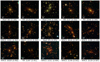 |
Fig. 1. Colour-composite images of the 15 clusters included in our analysis, obtained by combining HST bands from optical to near IR. The images are squared cut-outs, ∼130″ across, centred on the cluster core. |
For each spectroscopic source within the HST images, we extracted a squared cut-out with a side of ∼4″ (64 pixels), centered on the source position. A sample of the dataset is shown in Fig. 2, where CLMs were extracted from five clusters: Abell 383 (A383, z = 0.188), RX J2248-44311 (R2248, z = 0.346), MACS J0416-2403 (M0416, z = 0.397), MACS J1206-0847 (M1206, z = 0.439), and MACS J1149+2223 (M1149, z = 0.542). Due to different pointing strategies and the fields of view of HST cameras, many sources do not have a complete photometric coverage, especially in the IR range. As a result, these objects with missing information were not useful for the training process (Batista & Monard 2003; Marlin 2008; Parker 2010). With the aim of maximising the number of training samples with available spectroscopic redshift information, we chose four different band configurations:
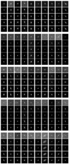 |
Fig. 2. Examples of cut-outs of cluster members extracted from HST images (F435, F606, F814, F105, F140 bands), corresponding to five clusters (from top to bottom): A383 (z = 0.188), R2248 (z = 0.346), M0416 (z = 0.397), M1206 (z = 0.439), M1149 (z = 0.542). All the cut-outs are 4 arcsec across. |
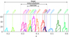 |
Fig. 3. Redshift distribution of 1629 spectroscopic members used for the EXP2 configuration. The three clusters A370 (z = 0.375, 224 CLMs), MS2137 (z = 0.316, 45 CLMs) and M0329 (z = 0.450, 74 CLMs) are used as blind test set. |
– ACS: only the seven optical bands (i.e. F435, F475, F606, F625, F775, F814, F850) were included in the training set, obtaining 1603 CLMs and 1899 NCLMs;
– ALL: the training set involved all twelve bands (i.e. the seven optical bands and the five IR bands F105, F110, F125, F140, F160), thus reducing the number of objects to 1156 and 1425, respectively for CLMs and NCLMs, due to the rejection of missing data;
– Mixed: we selected five bands, corresponding to the filters available in the Hubble Frontier Fields survey, covering the optical-IR range, namely, F435, F606, F814, F105, F140, respectively. This includes 1249 CLMs and 1571 NCLMs;
– Mixed*: same band combination as in the previous case (mixed), but including two further clusters, namely, Abell 2744 (A2744) and Abell 370 (A370), for which only HFF imaging were available. This set is composed of 1629 CLMs and 2161 NCLMs.
In practice, the three configurations, ACS, ALL and mixed, share the same clusters, while exploring different spectral information by varying the number of sources. The mixed* configuration considers an augmented cluster data set by including additional spectroscopic members. A summary of the cluster sample and the spectroscopic data sets is given in Table 1.
3. Methodology
In this work, we discuss the results achieved by a VGGNET-like2 model, which is a CNN implementation inspired by the VGG network proposed by Simonyan & Zisserman (2014).
As is customary in applications of ML methods, the data require a preparation phase, which, in this case, consisted of a data augmentation procedure, that is meant to construct a consistent labelled sample, followed by a partitioning of the dataset into training, validation, and blind testing sets.
Regarding data augmentation, given the relatively small sample of spectroscopic sources with respect to the typical size of the knowledge base required by supervised ML experiments, we increased the training set by adding images of spectroscopic sources, obtained from the original ones, through rotations and flips. The inclusion of these images in the training set also offered the possibility to make the network invariant to these operations, which works as an advantage for astronomical images as there is no defined orientation for the observed sources.
Concerning the partitioning of the data set, in order to fully cover the input parameter space, we opted for a stratified k-fold partitioning approach (Hastie et al. 2009; Kohavi 1995): the whole data set was split into k = 10 non-overlapping folds, of which, iteratively, one extracted subset was used as a blind test set, while the others were taken as a training set. Such an approach has several advantages: (i) increase of the statistical significance of the test set; (ii) the blind test is performed only on original images; and (iii) complete coverage of both training and test sets, keeping them well-separated at the same time.
The classification performance, obtained through all the experiments performed by this procedure, was evaluated by adopting a set of statistical estimators, directly derived from the classification confusion matrix (Stehman 1997), namely, the classification efficiency (AE), averaged over the two classes (members and non-members), the purity (pur), the completeness (comp), and the harmonic mean of purity and completeness (F1, see Appendix A.3). The last three estimators have been measured for each class. Completeness (also known as recall) and purity (also known as precision) are the most interesting estimators, suitable for measuring the quality of the classification performed by any method. The completeness, in fact, measures the capability to extract a “complete” set of candidates of a given class, while purity estimates the capability of selecting a “pure” set of candidates (thus, minimising the contamination). Therefore, the classification quality is usually based on either one of such two estimators or their combination, depending on the specific interest of an experiment (D’Isanto et al. 2016). In our case, we were most interested in finding the best trade-off between both estimators for the cluster members. The statistical evaluation was completed by also using the receiver operating characteristic curve (ROC, Hanley & McNeil 1982), which is a diagram where the true positive rate (TPR, i.e. the completeness rate) is plotted versus the false positive rate (FPR, i.e. the contamination rate, which corresponds to 1-purity) by varying the membership probability threshold. The model performances are measured in terms of the area under the curve (AUC), thus providing an aggregate measure of performance across all possible classification thresholds.
A full description of the data preparation procedure and the statistical estimators is given in Appendix A, while details about the architecture and configuration of the DL model are reported in Appendix B.
4. Experiments
In this section, we describe several experiments designed to test the performance of the CNNs and other methods. Specifically, with the data described in Sect. 2, we performed the following tests or experiments:
– EXP1: efficiency of the DL approach by stacking the data of all the clusters in terms of:
-
EXP1a: global evaluation
-
EXP1b: redshift-dependence, namely separating CLMs into redshift bins;
– EXP2: magnitude or colour dependence, by stacking data of a group of three clusters and varying their redshift range through:
-
EXP2a: separating bright and faint sources
-
EXP2b: separating red and blue galaxies
– EXP3: a comparison of performances of our image-based CNN technique with other approaches, based on photometric measurements of field and cluster galaxies.
4.1. EXP1: Combination of all clusters
At the first stage, we evaluated the global efficiency of a DL approach including all the available clusters, regardless of their redshift (ranging between 0.2 and 0.6), by exploring different combinations of photometric bands (as described in Sect. 2) and assembling the data set by stacking the information from all the images extracted from our cluster sample. We wanted to verify that DL models, given their intrinsic generalisation capabilities, were able to learn how to disentangle cluster members from non-member (foreground or background) sources, independently from the cluster redshift (EXP1a). This although their members have different characteristics, such as apparent magnitudes or sizes, and also different signal-to-noise ratio at a fixed apparent magnitude, due to the different image depths. The results are shown in Fig. 4 and Table D.1, as a function of the band configuration, described in Sect. 2.
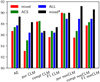 |
Fig. 4. Performance percentages of the CNN in the EXP1 experiment with the four band configurations (see Sect. 2) in terms of the statistical estimators described in Appendix A.3. |
For NCLM, we found similar values of the average efficiency (87%−89%), the purity (stable around ∼90%) and the F1-score (with variations within 1.5%), regardless of band configuration. On the other hand, the CLM identification was, in general, characterised by larger variation (83%−91%) in the statistical estimators. With the mixed* configuration, CNN achieved the best performances for CLM and it was also very stable in terms of NCLM, reaching an overall efficiency of ∼89%.
We also show, in Appendix D.1, the estimators obtained for each cluster (Table D.2 and Fig. D.1). This analysis confirmed that the mixed* combination showed the highest statistical values for all the thirteen clusters. Moreover, as expected, we demonstrated that there is a clear improvement of classification capabilities as the number of sources increases (an accuracy gain of ∼2.3% for an increment of 500 samples). Furthermore, fluctuations of these estimators tend to be better constrained for a large set of objects, stabilising around 3% when the number of samples is ≥2000 and showing an average reduction of ∼9% by quadrupling the number of sources.
Since the training set we used in this study was composed of galaxies spanning a large redshift range, as part of EXP1, we investigated whether any dependence on redshift is present. To this aim, the CLM redshift range was split into five equal-sized bins (∼280 samples). The performances and fluctuations related to the mixed* band combination are shown in Fig. 5, while details on the metrics are given in Table D.3. Despite the dissimilarities between galaxies at different depths, the CNN did not seem to be affected by the CLM redshift. In fact, CNN performances achieved in different redshift bins were all comparable, with a dispersion included within 0.04 − 1σ for the 65% of cross-compared estimator pairs and a mean separation of ∼0.8σ.
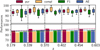 |
Fig. 5. Percentages of CNN classification results for the four statistical estimators, measured as a function of CLM redshift range (EXP1). The top panel describes their fluctuation in each bin, with the boxes delimiting the 25th and 75th percentiles (first and third quartile) and error bars enclosing the maximum point variations. The bottom panel shows the same metrics globally evaluated in each redshift bin, together with the best-fit lines. |
Since the mixed* band combinations provided the best results, all further experiments in the next sections refer to this band configuration.
4.2. EXP2: Selection of clusters as blind test set
A second set of experiments was devoted to the study of the CNN capability to predict cluster membership of sources belonging to clusters that are not included in the training set, that is, avoiding having member galaxies belonging to the same cluster populating both the training and test sets. Thus, we considered A370 (z = 0.375), MS 2137-2353 (MS2137, z = 0.316), and MACS J0329-0211 (M0329, z = 0.450) as blind test clusters, while the remaining clusters were organised into three different training sets based on different redshift ranges, as shown in Fig. 3. Specifically:
– Narrow: clusters with redshift 0.332 ≤ z ≤ 0.412 (514 CLMs, 555 NCLMs)
– Intermediate: clusters with redshift 0.286 ≤ z ≤ 0.467 (898 CLMs, 1157 NCLMs)
– Large: clusters with redshift 0.174 ≤ z ≤ 0.606 (1286 CLMs, 1725 NCLMs).
The training set configurations were mostly organised to identify CLMs in A370. This is the most significant test bench since it includes 535 spectroscopic sources and is in the middle of CLM redshift range. The other two clusters, MS2137 and M0329, were chosen as additional test sets located at redshifts lying outside the narrow and intermediate ranges, while remaining well within the large training set.
The results are shown Fig. 6 and detailed in Table D.4. They show that: (i) the large training set reached best results in most cases, with an average improvement between 1.1% and 4.3% with respect to the intermediate case; (ii) the narrow training ensemble provided, in most cases, the worst results, showing a lower trade-off between purity and completeness, particularly evident (larger than 3σ) for A370 and M0329. This confirmed that the best performances were reached by extending the knowledge base, that is, when the CLM training sample covers the largest available redshift range.
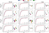 |
Fig. 6. Summary of the EXP2 experiment. The statistical performances for the three clusters (A370, M0329 and MS2137) are reported in each row, while results for the three training configurations (i.e. narrow, intermediate and large) are organised by column. The global performances achieved by stacking together the three clusters are reported in the bottom row. For each test set, we display the ROC curves (grey lines refer to the performances achieved by any training fold, while the main trend is emphasised in red, together with its AUC score); the box plots represent the fluctuation of measured estimators related to the CLMs, together with the average efficiency measured for both classes. As in Fig. 5, such boxes delimit the 25th and 75th percentiles, while error bars enclose the maximum point variations. |
We also analysed the CNN classification performances separately on bright and faint (EXP2a) galaxies, as well as on red and blue galaxies (EXP2b). The magnitude values adopted to split the CLM into equally sized samples are F814 = 22.0, 21.7, and 21.6 mag for A370, M0329, and MS2137, respectively. For the analysis of the colour dependence, we used the (F814 − F160) colour. However, since this colour depends on the F814 magnitude, we defined the difference between the observed colour and the colour-magnitude relation, that is, (F814 − F160)diff = (F814 − F160)obs− [colour–magnitude(F814)]. The colour-magnitude relation was fitted for each cluster with spectroscopic confirmed members, using a robust linear regression (Cappellari et al. 2013), which is a technique that allows for a possible intrinsic data scatter and clips outliers, adopting the least trimmed squares technique (Rousseeuw & Driessen 2006). By applying the correction for the colour-magnitude, we found that blue members can be defined as galaxies having (F814 − F160)diff < −0.160, −0.165, −0.157 for A370, M0329, and MS2137, respectively. Both experiments (a and b) were performed using the large redshift configuration.
The results of the CLM identification are shown in Table 2. In EXP2a, all the statistical estimators indicated a very good performance of the method, although with a slightly lower efficiency in identifying faint objects. In fact, brighter members were detected with higher completeness (90%−98%) and purity (81%−91%), with a significant F1 score improvement (89%−92%), when compared to fainter members (completeness: 80%−85%; purity: 77%−85%; F1 score: 78%−83%), obtaining remarkable results for A370, in which purity and completeness of CLMs are ∼88% and ∼97%, respectively. Nevertheless, fainter CLMs were identified with an acceptable F1 score (∼80%).
Statistical performances of the CNN model in EXP2.
The experiment, EXP2b, also showed good performances of the method for both red and blue objects, although the colour dependence of the results was evident. In particular, red galaxies were classified with a mean F1 score of ∼91%, decreasing down to ∼77% for blue objects. The results reflect the underlying similarity between blue members and background objects, which implies that they cannot be separated easily. This was confirmed by the analysis of false positives and false negatives discussed in Sect. 6.
4.3. EXP3: Comparison with photometric approaches
This section is dedicated to a comparison of the classification performance of cluster members using the image-based DL method described above along with two different techniques based on photometric catalogues. The first is a random forest classifier (developed by our team) and the second one is a photometry-based Bayesian model described in Grillo et al. (2015) and in Appendix C.
In this experiment, our CNN was trained with the mixed* filter set (see Sect. 2). We focused on the results obtained by these three methods on R2248, M0416, M1206, and M1149. The statistical estimators are shown in detail in Table D.5 and in Fig. D.3 as ROC curves, while in Fig. 7, the performances are summarised by combining the results from the four clusters based on their ROC curves (top), the trade-off between purity and completeness (middle), and the usual statistical estimators (bottom). The photometric techniques show an average efficiency around 86 − 89%, with some values ≳96% for the Bayesian approach, although the F1 scores always remain between 83% and 88%. The CNN confirmed its ability to detect CLMs with an F1 score between 87% and 91%. The upper panel in Fig. 7 shows that globally CNN reaches an AUC of ∼94%, which is ∼8% higher than the Bayesian method, while exhibiting the sharpest rise and the highest plateau. This means that for the CNN method there is a larger probability range in which the performances remain stable, while for the other methods a fine-tuning of the probability value is needed to balance purity and completeness. Furthermore, CNN reached the best trade-off between purity and completeness with a cross-over at ∼89%. A summary of the results is shown in the bottom panel of Fig. 7, where the differences among the CNN and the two photometric methods are measured using the four statistical estimators. The CNN performances were overall near 90% and remained consistently higher than those of photometric-based methods. Finally, we analysed the common predictions among the three methods, both in terms of correctly classified and misclassified sources, separately for CLMs and NCLMs. Such results are graphically represented in Fig. D.2. All three methods share ∼76% of their commonalities (i.e. summing of correct and incorrect predictions), of which, ∼97% (i.e. 74.6% with respect to the whole set of common sources) were correctly classified. Common true positives and true negatives (i.e. CLMs and NCLMs that have been correctly classified) were ∼75%. The CNN and Bayesian method shared the largest fraction of predictions ∼90% (of which ∼93% were correct) with respect to the joint classification of CNN and RF (∼82%); this implied that RF had a significant fraction of uncommon predictions (∼14%).
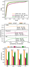 |
Fig. 7. Comparison among the image-based CNN and two photometric catalogue-based approaches, namely, a random forest and Bayesian method (EXP3), by combining results from the four clusters (R2248, M0416, M1206, M1149). Upper panel shows the ROC curves for the three methods with measured Area Under the Curve (AUC). The middle panel reports the trends of purity and completeness as a function of the probability thresholds used to obtain the ROC curves. In the three diagrams, we mark the intersection between such curves, i.e. the probability for which completeness and purity are equal. Bottom panel shows the differences between the three methods based on the statistical estimators described in Appendix A.3. |
Concerning the misclassified objects, the methods shared ∼2% of incorrect predictions, of which: ∼1% of CLMs were common false negatives (FNs, i.e. CLMs sources wrongly predicted as NCLMs), while 2.5% were common false positives (FPs, i.e. NCLMs sources wrongly predicted as CLMs). The CNN exhibited the least fraction of misclassifications (about 10%). The CNN showed a percentage of FNs larger than Bayesian (10% versus 7%), which, in turn, had a wider FP rate (11% versus 17%). Therefore, although CNN and Bayesian methods shared a significant fraction of incorrect predictions (85% of common misclassifications, suggesting the existence of a fraction of sources for which the membership is particularly complex for both of them), these two models exhibit a different behaviour: the CNN tended to produce more pure than complete CLMs samples, whereas the Bayesian method showed the opposite, which is in agreement with what is reported in Table D.5.
5. Photometric selection of CLMs
The experiments described in the previous sections are mostly focused on the classification efficiency and limits of the image-based CNN approach and evaluating its dependence from observational parameters such as redshift, number of CLM, photometric band compositions, magnitude, and colour. In this section, we are mainly interested in evaluating the degree of generalisation capability of the trained CNN in classifying new sources as cluster members, a step process that is commonly referred to as run in the ML context.
In particular, we applied the CNN model to the photometrically selected CLMs in R2248, M0416, M1206, and M1149. The training set was constructed by combining all clusters with the mixed* band configuration, using the k-fold approach (see Sect. 3).
Similarly to what was done to build the knowledge base (see Sect. 2), for the run set we used squared cut-outs ∼4″ across, centered on the source positions as extracted by SExtractor (Bertin & Arnouts 1996). Thus, the run set was composed by 5269 unknown sources, of which 1286, 1029, 1246, and 1708 were in the FoV of R2248, M0416, M1206, and M1149, respectively.
The CNN identified a total of 372 members with F814 ≤ 25 mag, which is approximately the magnitude limit of the spectroscopic members (only ∼3% of spectroscopic members has F814 > 25), with ∼46% of candidate CLMs having membership probabilities larger than 90%. The spatial distribution of both spectroscopic and predicted CLMs are shown in Fig. 8, while the magnitude (F814) distribution and the colour-magnitude relations (F606 − F814 versus F814) for both spectroscopic and predicted members are shown in Fig. 9. The magnitude distributions indicate that the CNN was able to complete the spectroscopic CLMs sample down to F814 = 25. This was also confirmed by the analysis of the colour-magnitude diagrams, which show that the photometrically identified CLMs complete the spectroscopic red-sequence at F814 < 25, emphasising the CNN capability to disentangle CLMs from background objects. We counted also the number of recognised CLMs within, respectively, 1, 2, and 3σ from the median of differential colour (F606 − F814)diff.
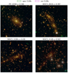 |
Fig. 8. CNN member selection (marked with open magenta squares) obtained with the run set, together with the spectroscopic CLMs (marked with open green squares), in the core of the four clusters R2248 (z = 0.346), M0416 (z = 0.397), M1206 (z = 0.439) and M1149 (z = 0.542). All images are 130 arcsec across. |
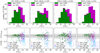 |
Fig. 9. CNN membership prediction (run) together with spectroscopic sources, represented as (i) CLMs distribution of F814 magnitudes (first row), (ii) differential colour – magnitude sequence for both CLMs and NCLMs. Spectroscopic CLMs are shown in green, candidate members in purple, spectroscopic NCLMs with blue squares and candidate NCLMs with open cyan circle. We only plot CNN cluster members with F814 ≤ 25 mag. The grey region within the CM diagrams limits the area corresponding to ±1σ from the median (dashed horizontal line) of (F606 − F814)diff. |
6. Discussion
One particular aspect that is often addressed when using ML methods is the impact on the classification performances carried by the amount of data available, both in terms of the number of features (photometric bands) and amount of training objects. The EXP1 (see Sect. 4.1) enabled an analysis of the trade-off between the information carried by the imaging bands and the number of samples in the dataset. As reported in Table D.1 and Table D.2, there was a small improvement of efficiency (∼3%) by increasing the size of the training sample by 34%, when comparing the two mixed and mixed* configurations. However, these two data samples included both optical and infrared information. To better understand this important aspect, we performed a comparison between data samples with and without the infrared bands. Such analysis was carried out by directly comparing the two ACS and ALL configurations, although the sample size of the second one was ∼30% smaller. The results, shown in Table D.1 and Table D.2, suggested that the addition of infrared imaging adequately compensated the smaller size of the training set.
We also investigated the dependence of member classification performance on the magnitudes and colours. Here, the EXP2a showed very good performances of the method for both bright and faint sources, although with a slightly lower efficiency in identifying fainter objects. On the other hand, EXP2b showed a mean efficiency of ∼91% in classifying red galaxies, which was reduced to ∼77% for blue objects (see Table 2).
To further investigate the robustness in the identification of cluster members (i.e. the positive class), from the classification confusion matrices, we defined true positives (TPs) the CLMs correctly classified, false positives (FPs) NCLMs classified as CLMs, false negatives (FNs) the CLMs classified as NCLMs, and, finally, true negatives (TNs) as NCLMs correctly classified. A short sample of TPs, FPs and FNs in R2248 and M0416, and in M1206 and M1149 are shown in Figs. 10 and 11, respectively. We explored the model predictions, by inspecting the TPs and the distribution of FPs and FNs as function of their magnitude and colour.
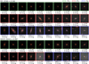 |
Fig. 10. Ensemble of object cut-outs with a size of 64 pixels (∼4″), corresponding to some specific CNN predictions in the clusters R2248 (first three rows) and M0416 (last two rows). The True Positives (TPs), i.e. the CLMs correctly identified, are shown on first and fourth row with green boxes, while False Positive and False Negative (FPs and FNs) are shown on the second, third and fifth row, framed by red and blue boxes, respectively. The images were obtained by combining five HST bands: F435, F606, F814, F105, F140. The figure shows sources in the F814 band with a magnitude F814 ≤ 25 mag. TPs are shown together with their spectroscopic redshift, while FNs together with their cluster rest-frame velocity separation. For convenience, in the case of FPs, their cluster velocity separations are quoted when within ±9000 km s−1, otherwise their redshift is shown. |
A critical aspect of the classification of members within the central cluster region is the impact of crowding. Therefore, we specifically focused on the DL ability to predict cluster membership in such circumstances (see a few examples of cut-outs in Figs. 10 and 11).
We introduced a contamination index (CI) for each cut-out, defined as:  , where Nc is the number of contaminants in the cut-outs, di is the distance in arcsec between the central source and i−th contaminant, while F814i is the magnitude of the contaminating source. The indices for cut-outs without contaminants were set to zero. Then, we normalised this index in the [0, 1] interval. Figure 12 shows that the four contamination index distributions of, respectively, TPs, TNs, FPs and FNs mostly overlapped and followed the same trend. In fact, the 48% of FNs and 28% of FPs had a non-zero contamination index, as well as the 31% and 43% of TNs and TPs. The lack of a correlation between the contamination index and incorrect prediction rates (FPs and FNs) suggests that the source crowding did not significantly affect the CNN classification efficiency.
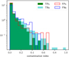 |
Fig. 12. Logarithmic distribution of the contamination index for true positives (TPs, green), true negatives (cyan), false positives (red), and false negatives (blue). The distribution includes all available clusters. |
By analysing the FP and FN rows in Figs. 10 and 11, we can see an interesting dichotomy: FPs appear as red galaxies, while FNs as blue; in addition, the FPs have F814 < 24, whereas FNs are found also down to F814 ∼ 25. In order to quantify such behaviours, we analysed the distribution of FPs and FNs in terms of: (i) the F814 magnitude for both FPs and FNs (Fig. 13a); (ii) the correlation between the CNN incorrect predictions and differential colours (F606 − F814)diff (Fig. 13b). These results are summarised in Table 3.
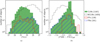 |
Fig. 13. Magnitude (left panel) and colour (right panel) logarithmic distributions of FPs (red) and FNs (blue), overlapped to the CLM (green) and NCLM distributions, for the fifteen clusters (stacked) included in our study. The number of objects for each plotted distribution is quoted in brackets in the legend. The differential colour (F606 − F814)diff is obtained by applying the correction for the mean colour-magnitude relation for each cluster. Table 3 outlines such results. |
Summary of FP and FN distributions.
Figure 13a and Col. 4 in Table 3 showed that almost all CLMs fainter than F814W = 25 (representing a small fraction with respect to the total, see Col. 2 in Table 3) were FNs. This was not due to any failure on the part of the model, but, rather, to the poor sampling of such objects within the parameter space available to train the model. This was also confirmed when comparing the percentage of FPs and FNs with respect to the percentage of CLMs and NCLMs in Table 3 as a function of magnitude. In fact, Table 3 showed that the model tried to reproduce the distribution in terms of fractions of CLMs for FPs, and in terms of the fraction of NCLMs for FNs.
Finally, we analysed the correlations between the CNN incorrect predictions and colours. These distributions are shown in Fig. 13b using the differential colour (F606 − F814)diff, while, in Table 3, the misclassification percentages are summarised. Also in this case, the distributions of FPs and FNs as a function of colours, are mimicking, respectively, the distributions of CLMs and NCLMs in Table 3.
Very blue sources ((F606 − F814)diff < −0.5) populated only 5.8% of CLMs and represented the ∼35.4% of incorrect predictions, which is very similar to the fraction of very blue sources in the population of NCLMs (i.e. 43.2%). Conversely, redder sources were typically correctly classified, showing a FN rate of 16.6%. Moreover, from the fraction of FN/CLMs, we observed that almost all the blue cluster members were wrongly classified as NCLMs (see Col. 4 in Table 3 and Fig. 13b).
Regarding FPs, there was not a real classification problem with faint and very blue objects, whose rates in terms of CLMs were, respectively, 3.4% and 5.8%, corresponding to 2.2% and 4.3% of incorrect predictions, respectively. From Table 3, it was also evident that within red misclassifications, FPs were more frequent than FNs (29.5% versus 16.6%), reproducing the distributions of CLMs (39.2%) and NCLMs (15.4%), respectively.
Figure 14 shows the colour-magnitude relation of CLMs (green squares), overlapping the FP (red cross), FN (blue cross) and NCLM (grey circle) distributions. It emphasises the CLMs undersampling of the blue and faint region, together with the large concentration of FNs among bluer and fainter sources (see blue crosses). Among all the FNs, ∼35% are very blue ((F606 − F814)diff < −0.5), ∼40% of these had F814 > 25 mag, suggesting that in the bluer region the FNs follows the NCLM distribution, while among FPs, ∼64% of them are red ((F606 − F814)diff > −0.1), but only ∼1% of these have magnitude fainter than F814 > 25 mag. On the other hand, ∼35% of all FPs were within the yellow contours, which refer to the 1σ colour-magnitude relation, indicating that they were on the red sequence.
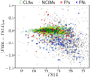 |
Fig. 14. Colour-magnitude relation for the CLMs (green squares), with the overlapped distributions of FPs (red crosses), FNs (blue crosses) and NCLMs (grey circles), for the sample of fifteen clusters (stacked). The yellow contour delimits the red-sequence at 1σ confidence level. Colours reported on the y-axis are corrected for the mean red-sequence of each cluster (see Sect. 4). |
In order to understand the impact of this misclassification of faint and very blue sources, we report, in Table 4, the statistical estimators for the stacked sample and, individually for R2248, M0416, M1206, M1149), considering either the whole sample or by removing sources with F814 > 25 and very blue objects, that is, with (F606 − F814)diff < −0.5. By comparing these results, we observed a relevant increase of the completeness (for the stacked sample, it goes from 84.8% to 90.8%). This was mainly motivated by the sensible reduction of the FNs amount, which, by definition, had a higher impact on the completeness, rather than on other estimators. In fact, the purity and F1 score showed a smaller improvement, going, respectively, from 87.9% to 88.4% and from 86.3% to 88.9%.
Comparison among CNN performances considering the whole sample (Col. 2) and by removing sources with F814 ≥ 25 and (F606 − F814)diff < −0.5 (Col. 3).
In summary, the FNs were mainly blue and faint. This was expected, given their under-representation in the dataset and their similarity with NCLMs. We note, in fact, that we were mapping a population of cluster members in the central and highest density region of clusters, dominated by a high fraction of bright and red members. Nevertheless, the simple exclusion of fainter sources with F814 > 25 and (F606 − F814)diff < −0.5 improved the CNN performance. Similar performances in terms of the distribution of false positives and negatives for sources with F814 > 25 and (F606 − F814)diff < −0.5 were obtained by the random forest classifier and the photometry-based Bayesian method. By comparing the behaviour of these three models on four clusters (R2248, M0416, M1206 and M1149), we found that the rate of blue FN is 28% for the Bayesian method and 25% for the random forest versus the 20% for the CNN. The rate of faint FN is 1% for the random forest and 6% for the Bayesian method versus the 5% of CNN. For what concerns FPs, the CNN, being the purest method, preserved the lowest contamination for both bluer and fainter members, with only four NCLMs classified as CLMs, compared with the 12 and 24 NCLMs for the Bayesian method and the random forest, respectively.
This comparison, while it confirms the good performances of the CNN, also shows that the three methods have comparable efficiencies in the faint and blue region of the parameter space, which is likely due to undersampling of members in this region of the knowledge base, as pointed out above. This is due to the fact that the population of galaxies in the densest central cluster regions is brighter and redder than that of the less dense and outer cluster regions (see Annunziatella et al. 2014; Mercurio et al. 2016 for the specific study of M1206). Clearly, an improvement of the model’s performances would require including member galaxies in the outer cluster regions and balancing the number of bluer and fainter members. In our case, even if the spectroscopic data cover more than two cluster virial radii, multi-band HST imaging with sufficient depth is only available in the central cluster regions.
Finally, we used both spectroscopic members and candidate CLMs identified by CNN to estimate the cumulative projected number of cluster members and the differential number density profiles (Fig. 15). According to our previous analysis, we excluded candidate CLMs with F814 > 25 mag, where only ∼3% of spectroscopic members were present. To properly compare profiles of clusters with different virial masses, we computed the values R200 from of the values of M200c obtained by Umetsu et al. (2018) with independent weak lensing measurements3. We then computed all profiles as a function of the projected radius in units of R200 and rescaled them by the number of members, N0, found within the radius R/R200 = 0.15 in each cluster. In Fig. 15, we showed the cumulative projected number and the differential projected number density profiles of cluster members after applying such renormalisations, where the shaded areas correspond to 68% confidence levels. Interestingly, we found that the radial distributions of all clusters followed a universal profile, including M0416, which is an asymmetric merging cluster. We noted that a similar homology relation among rescaled projected mass profiles was found in Bonamigo et al. (2018) and Caminha et al. (2019), using strong lensing modelling. This result confirms that our methodology was able to identify the CLM population with a high degree of purity and completeness.
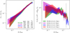 |
Fig. 15. Cumulative (left) and differential (right) projected number of CLM for the four clusters (R2248, M0416, M1206, and M1149), including spectroscopic CLMs and candidate members identified by CNN (limited to F814 ≤ 25 mag). The areas correspond to the 68% confidence level regions. All profiles are normalised by the number N0 of members with R < 0.15 R200 in all clusters. The number of spectroscopic, CNN-identified members (“run”), and N0 values are quoted in the left panel. The adopted values of R200 are quoted in the right panel, the computed values of N0 are quoted in the left panel, together with the corresponding numbers of spectroscopic and “run” members. The dashed line in the right panel corresponds to R = 0.15 R200. |
7. Conclusions
In this work, we carry out a detailed analysis of CNN capabilities to identify members in galaxy clusters, disentangling them from foreground and background objects, based on imaging data alone. Such a methodology, therefore, avoided the time consuming and challenging task of building photometric catalogues in cluster cores. We used OPT-NIR high quality HST images, supported by MUSE and CLASH-VLT spectroscopic observations of fifteen clusters, spanning the redshift range zcluster = (0.19, 0.60).
We used this extensive spectroscopic coverage to build a training set by combining CLMs and NCLMs. We performed three experiments by consecutively varying the HST band combinations and the set of training clusters to study the dependence of DL efficiency on (i) the cluster redshift (EXP1); and (ii) the magnitude and colour of cluster galaxies (EXP2). We also compared the CNN performance with other methods (random forest and Bayesian model), based instead on photometric measurements (EXP3). The main results can be summarised as follows:
-
Despite members belonging to clusters spanning a wide range of redshift, the CNN achieved a purity-completeness rate ≳90%, showing a stable behaviour and a remarkable generalisation capability over a relatively wide cluster redshift range (Sect. 4.1).
-
The CNN efficiency was maximised when a large set of sources was combined with HST passbands, including both optical and infrared information. The robustness of the trained model appeared reliable even when a subset of clusters was moved from the training to the blind test set, causing a small drop (< 5%) in performance. We observed some performance differences for bright and faint sources, as well as for red and blue galaxies. However, the results maintained the purity, completeness and F1 score greater than 72% (Table 2 in Sect. 4.2).
-
By using images, rather than photometric measurements, the CNN technique was able to identify CLMs with the lowest rate of contamination and the best trade-off between purity and completeness, when compared to photometry-based methods, which instead require a critical fine-tuning of the classification probability.
-
The false negatives, that is, the NCLMs wrongly classified as CLMs were mainly blue and faint. This was simply the result of their limited under-sampling in the training dataset, as well as their similarity with NCLMs. However, by excluding sources with F814 > 25 mag and (F606 − F814)diff < −0.5, the CNN performance improved significantly. These performances reflected the capability of the CNN to classify unknown objects, from which a highly complete and pure magnitude limited sample of candidate CLMs could be extracted for several different applications in the study of the galaxy populations and mass distribution of galaxy clusters via lensing techniques.
Therefore, based on an adequate spectroscopic survey of a limited sample of clusters as a training base, the proposed methodology can be considered a valid alternative to photometry-based methods, circumventing the time-consuming process of multi-band photometry, and working directly on multi-band imaging data in counts. To improve CNN performance to recognise the faintest and blue CLMs, it would be desirable to plan both HST and spectroscopic observations also covering control fields in the outer cluster regions, with the same depth and passbands as the central regions.
Furthermore, the generalisation capability of this kind of models makes them both versatile and reusable tools. In fact, the convolution layers of a trained deep network can be reused as shared layers in larger models, such as the Faster Region CNN (Ren et al. 2015) and Masked Region CNN (He et al. 2017), which exploit kernel weights to extract multidimensional information suitable to performing object detection. Such architectures have already found interesting astrophysical applications, for example, in the identification of radio sources (Wu et al. 2019) and the automatic deblending of astronomical sources (Burke et al. 2019).
In future works, we will extend this analysis to wide-field ground-based observations and explore other promising deep learning architectures, such as deep auto-encoders (Goodfellow 2010) and conditional generative adversarial networks (Mirza & Osindero 2014), to integrate the ground-based lower resolution images with the high quality of HST images in cluster fields. We also plan to investigate new techniques to overcome the problem of missing data, thus increasing the size of the training set with a more homogeneous sampling of the entire parameter space.
We tested different network architectures, e.g. Residual Net X (He et al. 2015; Xie et al. 2016) and Inception Net (Szegedy et al. 2014). Due to their lower performances, we limited the description of the results to the VGGNET-like model, to avoid weighing down the text.
Acknowledgments
The authors thank the anonymous referee for the very useful comments and suggestions. The software package HIGHCoOLS (Hierarchical Generative Hidden Convolution Optimization System, http://dame.oacn.inaf.it/highcools.html), developed within the DAME project (Brescia et al. 2014), has been used for the deep learning models described in this work. We acknowledge funding by PRIN-MIUR 2017WSCC32 “Zooming into dark matter and proto-galaxies with massive lensing clusters”, INAF mainstream 1.05.01.86.20: “Deep and wide view of galaxy clusters (ref. Mario Nonino)” and INAF mainstream 1.05.01.86.31 (ref. Eros Vanzella). MB acknowledges financial contributions from the agreement ASI/INAF 2018-23-HH.0, Euclid ESA mission – Phase D and with AM the INAF PRIN-SKA 2017 program 1.05.01.88.04. CG acknowledges support through Grant no. 10123 of the VILLUM FONDEN Young Investigator Programme. In this work several public software was used: Topcat (Taylor 2005), Astropy (Astropy Collaboration 2013, 2018), TensorFlow (Abadi et al. 2015), Keras (Chollet 2015) and Scikit-Learn (Pedregosa et al. 2011).
References
- Abadi, M., Agarwal, A., Barham, P., et al. 2015, TensorFlow: Large-Scale Machine Learning on Heterogeneous Systems, software available from tensorflow.org (San Francisco: Astronomical Society of the Pacific) [Google Scholar]
- Annunziatella, M., Biviano, A., Mercurio, A., et al. 2014, A&A, 571, A80 [NASA ADS] [CrossRef] [EDP Sciences] [Google Scholar]
- Annunziatella, M., Mercurio, A., Biviano, A., et al. 2016, A&A, 585, A160 [NASA ADS] [CrossRef] [EDP Sciences] [Google Scholar]
- Annunziatella, M., Bonamigo, M., Grillo, C., et al. 2017, ApJ, 851, 81 [NASA ADS] [CrossRef] [Google Scholar]
- Astropy Collaboration (Robitaille, T. P., et al.) 2013, A&A, 558, A33 [NASA ADS] [CrossRef] [EDP Sciences] [Google Scholar]
- Astropy Collaboration (Price-Whelan, A. M., et al.) 2018, AJ, 156, 123 [Google Scholar]
- Bacon, R., Vernet, J., Borisova, E., et al. 2014, Messenger, 157, 13 [Google Scholar]
- Balestra, I., Mercurio, A., Sartoris, B., et al. 2016, ApJS, 224, 33 [Google Scholar]
- Batista, G. E. A. P. A., & Monard, M. C. 2003, Appl. Artif. Intell., 17, 519 [CrossRef] [Google Scholar]
- Bengio, Y. 2012, Neural networks: Tricks of trade, Springer, 437 [CrossRef] [Google Scholar]
- Bergamini, P., Rosati, P., Mercurio, A., et al. 2019, A&A, 631, A130 [NASA ADS] [CrossRef] [EDP Sciences] [Google Scholar]
- Bertin, E., & Arnouts, S. 1996, Ap&SS, 117, 393 [Google Scholar]
- Bishop, C. M. 2006, Pattern Recognition and Machine Learning (Information Science and Statistics) (Secaucus, NJ, USA: Springer-Verlag, New York, Inc.) [Google Scholar]
- Biviano, A., Rosati, P., Balestra, I., et al. 2013, A&A, 558, A1 [NASA ADS] [CrossRef] [EDP Sciences] [Google Scholar]
- Bonamigo, M., Grillo, C., Ettori, S., et al. 2018, ApJ, 864, 98 [NASA ADS] [CrossRef] [Google Scholar]
- Breiman, L. 2001, Mach. Learn., 45, 5 [CrossRef] [Google Scholar]
- Brescia, M., Cavuoti, S., D’Abrusco, R., Longo, G., & Mercurio, A. 2013, ApJ, 772, 140 [NASA ADS] [CrossRef] [Google Scholar]
- Brescia, M., Cavuoti, S., Longo, G., et al. 2014, PASP, 126, 783 [Google Scholar]
- Brescia, M., Cavuoti, S., Amaro, V., et al. 2018, in Data Analytics and Management in Data Intensive Domains, eds. L. Kalinichenko, Y. Manolopoulos, O. Malkov, et al. (Cham: Springer International Publishing), Commun. Comput. Inf. Sci., 822, 61 [CrossRef] [Google Scholar]
- Burke, C. J., Aleo, P. D., Chen, Y.-C., et al. 2019, MNRAS, 490, 3952 [CrossRef] [Google Scholar]
- Caminha, G. B., Grillo, C., Rosati, P., et al. 2016, A&A, 587, A80 [NASA ADS] [CrossRef] [EDP Sciences] [Google Scholar]
- Caminha, G. B., Grillo, C., Rosati, P., et al. 2017a, A&A, 600, A90 [NASA ADS] [CrossRef] [EDP Sciences] [Google Scholar]
- Caminha, G. B., Grillo, C., Rosati, P., et al. 2017b, A&A, 607, A93 [NASA ADS] [CrossRef] [EDP Sciences] [Google Scholar]
- Caminha, G. B., Rosati, P., Grillo, C., et al. 2019, A&A, 632, A36 [CrossRef] [EDP Sciences] [Google Scholar]
- Cappellari, M., Scott, N., Alatalo, K., et al. 2013, MNRAS, 432, 1709 [NASA ADS] [CrossRef] [Google Scholar]
- Cavuoti, S., Brescia, M., De Stefano, V., & Longo, G. 2015, Exp. Astron., 39, 45 [NASA ADS] [CrossRef] [Google Scholar]
- Chollet, F., et al. 2015, Keras, https://keras.io [Google Scholar]
- Coe, D., Umetsu, K., Zitrin, A., et al. 2012, ApJ, 757, 22 [NASA ADS] [CrossRef] [Google Scholar]
- Cui, X., Goel, V., & Kingsbury, B. 2015, IEEE/ACM Trans. Audio Speech Lang. Process., 23, 1469 [CrossRef] [Google Scholar]
- Devroye, L., Györfi, L., & Lugosi, G. 1996, in A Probabilistic Theory of Pattern Recognition, (Springer), Stochastic Modell. Appl. Probab., 31, 1 [CrossRef] [Google Scholar]
- Diemand, J., & Moore, B. 2011, Adv. Sci. Lett., 4, 297 [NASA ADS] [CrossRef] [Google Scholar]
- D’Isanto, A., Cavuoti, S., Brescia, M., et al. 2016, MNRAS, 457, 3119 [NASA ADS] [CrossRef] [Google Scholar]
- Duchi, J., Hazan, E., & Singer, Y. 2011, J. Mach. Learn. Res., 12, 2121 [Google Scholar]
- Girardi, M., Mercurio, A., Balestra, I., et al. 2015, A&A, 579, A4 [NASA ADS] [CrossRef] [EDP Sciences] [Google Scholar]
- Goodfellow, I. J. 2010, Technical Report: Multidimensional, Downsampled Convolution for Autoencoders, Tech. rep. (Université de Montréal) [Google Scholar]
- Goodfellow, I., Bengio, Y., & Courville, A. 2016, Deep Learning (MIT Press), http://www.deeplearningbook.org [Google Scholar]
- Grillo, C., Suyu, S. H., Rosati, P., et al. 2015, ApJ, 800, 38 [NASA ADS] [CrossRef] [Google Scholar]
- Grillo, C., Karman, W., Suyu, S. H., et al. 2016, ApJ, 822, 78 [NASA ADS] [CrossRef] [Google Scholar]
- Hanley, J. A., & McNeil, B. J. 1982, Radiology, 143, 29 [CrossRef] [PubMed] [Google Scholar]
- Hastie, T., Tibshirani, R., & Friedman, J. 2009, in The Elements of Statistical Learning: Data Mining, Inference, and Prediction, Second Edition, (New York: Springer), Springer Ser. Stat. [Google Scholar]
- He, K., Zhang, X., Ren, S., & Sun, J. 2015, ArXiv e-prints [arXiv:1512.03385] [Google Scholar]
- He, K., Gkioxari, G., Dollár, P., & Girshick, R. 2017, ArXiv e-prints [arXiv:1703.06870] [Google Scholar]
- Hebb, D. O. 1949, The Organization of Behavior: a Neuropsychological Theory/D. O. Hebb, xix (New York: Wiley), 335 [Google Scholar]
- Ho, M., Rau, M. M., Ntampaka, M., et al. 2019, ApJ, 887, 25 [NASA ADS] [CrossRef] [Google Scholar]
- Ivezić, Ž., Kahn, S. M., Tyson, J. A., et al. 2019, ApJ, 873, 111 [NASA ADS] [CrossRef] [Google Scholar]
- Kingma, D. P., & Ba, J. 2014, ArXiv e-prints [arXiv:1412.6980] [Google Scholar]
- Koekemoer, A. M., Aussel, H., Calzetti, D., et al. 2007, ApJS, 172, 196 [NASA ADS] [CrossRef] [Google Scholar]
- Koekemoer, A. M., Faber, S. M., Ferguson, H. C., et al. 2011, ApJS, 197, 36 [NASA ADS] [CrossRef] [Google Scholar]
- Kohavi, R. 1995, Proceedings of the 14th International Joint Conference on Artificial Intelligence - Volume 2, IJCAI’95 (San Francisco, CA, USA: Morgan Kaufmann Publishers Inc.), 1137 [Google Scholar]
- Lagattuta, D. J., Richard, J., Clément, B., et al. 2017, MNRAS, 469, 3946 [Google Scholar]
- Lagattuta, D. J., Richard, J., Bauer, F. E., et al. 2019, MNRAS, 485, 3738 [NASA ADS] [Google Scholar]
- Laureijs, R., Hoar, J., Buenadicha, G., et al. 2014, in The Euclid Mission: Cosmology Data Processing and Much More, (Astronomical Society of the Pacific), ASP Conf. Ser., 485, 495 [Google Scholar]
- LeCun, Y., Boser, B., Denker, J. S., et al. 1989, Neural Comput., 1, 541 [CrossRef] [Google Scholar]
- Lotz, J. M., Koekemoer, A., Coe, D., et al. 2017, ApJ, 837, 97 [Google Scholar]
- Maas, A. L., Hannun, A. Y., & Ng, A. Y. 2013, ICML Workshop on Deep Learning for Audio, Speech and Language Processing [Google Scholar]
- Mahler, G., Richard, J., Clément, B., et al. 2018, MNRAS, 473, 663 [NASA ADS] [CrossRef] [Google Scholar]
- Marlin, B. 2008, PhD Thesis, Department of Computer Science, University of Toronto [Google Scholar]
- Medezinski, E., Umetsu, K., Okabe, N., et al. 2016, ApJ, 817, 24 [NASA ADS] [CrossRef] [Google Scholar]
- Meneghetti, M., Davoli, G., Bergamini, P., et al. 2020, Science, 369, 1347 [Google Scholar]
- Mercurio, A., Annunziatella, M., Biviano, A., et al. 2016, in The Universe of Digital Sky Surveys, eds. N. R. Napolitano, G. Longo, M. Marconi, M. Paolillo, E. Iodice, et al., 42, 225 [CrossRef] [Google Scholar]
- Merten, J., Giocoli, C., Baldi, M., et al. 2019, MNRAS, 487, 104 [CrossRef] [Google Scholar]
- Mirza, M., & Osindero, S. 2014, ArXiv e-prints [arXiv:1411.1784] [Google Scholar]
- Molino, A., Benítez, N., Ascaso, B., et al. 2017, MNRAS, 470, 95 [NASA ADS] [CrossRef] [Google Scholar]
- Molino, A., Costa-Duarte, M. V., Mendes de Oliveira, C., et al. 2019, A&A, 622, A178 [NASA ADS] [CrossRef] [EDP Sciences] [Google Scholar]
- Monna, A., Seitz, S., Zitrin, A., et al. 2015, MNRAS, 447, 1224 [NASA ADS] [CrossRef] [Google Scholar]
- Ntampaka, M., Trac, H., Sutherland, D. J., et al. 2015, ApJ, 803, 50 [NASA ADS] [CrossRef] [Google Scholar]
- Ntampaka, M., Trac, H., Sutherland, D. J., et al. 2016, ApJ, 831, 135 [NASA ADS] [CrossRef] [Google Scholar]
- Ntampaka, M., ZuHone, J., Eisenstein, D., et al. 2019, ApJ, 876, 82 [CrossRef] [Google Scholar]
- Parker, R. 2010, Missing Data Problems in Machine Learning (VDM Verlag) [Google Scholar]
- Pedregosa, F., Varoquaux, G., Gramfort, A., et al. 2011, J. Mach. Learn. Res., 12, 2825 [Google Scholar]
- Perez, L., & Wang, J. 2017, ArXiv e-prints [arXiv:1712.04621] [Google Scholar]
- Postman, M., Coe, D., Benítez, N., et al. 2012, ApJS, 199, 25 [NASA ADS] [CrossRef] [Google Scholar]
- Prechelt, L. 1997, Neural Networks: Tricks of the Trade, volume 1524 of LNCS, Chapter 2 (Springer-Verlag), 55 [Google Scholar]
- Raskutti, G., Wainwright, M. J., & Yu, B. 2011, 49th Annual Allerton Conference on Communication, Control, and Computing (Allerton), 1318 [CrossRef] [Google Scholar]
- Ren, S., He, K., Girshick, R., & Sun, J. 2015, ArXiv e-prints [arXiv:1506.01497] [Google Scholar]
- Rosati, P., Balestra, I., Grillo, C., et al. 2014, Messenger, 158, 48 [Google Scholar]
- Rousseeuw, P. J. 1984, J. Am. Stat. Assoc., 79, 871 [CrossRef] [Google Scholar]
- Rousseeuw, P. J., & Driessen, K. 2006, Data Min. Knowl. Discov., 12, 29 [CrossRef] [Google Scholar]
- Simard, P. Y., Steinkrau, D., & Buck, I. 2005, Eighth International Conference on Document Analysis and Recognition (ICDAR’05)(ICDAR), 1115 [Google Scholar]
- Simonyan, K., & Zisserman, A. 2014, ArXiv e-prints [arXiv:1409.1556] [Google Scholar]
- Srivastava, N., Hinton, G., Krizhevsky, A., Sutskever, I., & Salakhutdinov, R. 2014, J. Mach. Learn. Res., 15, 1929 [Google Scholar]
- Stehman, S. V. 1997, Remote Sens. Environ., 62, 77 [CrossRef] [Google Scholar]
- Szegedy, C., Liu, W., Jia, Y., et al. 2014, ArXiv e-prints [arXiv:1409.4842] [Google Scholar]
- Taylor, M. B. 2005, in Astronomical Data Analysis Software and Systems XIV, eds. P. Shopbell, M. Britton, & R. Ebert, ASP Conf. Ser., 347, 29 [Google Scholar]
- Treu, T., Brammer, G., Diego, J. M., et al. 2016, ApJ, 817, 60 [NASA ADS] [CrossRef] [Google Scholar]
- Umetsu, K., Sereno, M., Tam, S.-I., et al. 2018, ApJ, 860, 104 [NASA ADS] [CrossRef] [Google Scholar]
- Wu, C., Wong, O. I., Rudnick, L., et al. 2019, MNRAS, 482, 1211 [NASA ADS] [CrossRef] [Google Scholar]
- Xie, S., Girshick, R., Dollár, P., Tu, Z., & He, K. 2016, ArXiv e-prints [arXiv:1611.05431] [Google Scholar]
- Zeiler, M. D. 2012, ArXiv e-prints [arXiv:1212.5701] [Google Scholar]
Appendix A: Methodology
The data preparation phase, preceding the application of the ML based classifiers, is organised as a series of pre-processing steps, detailed in the following sections.
A.1. Data augmentation
The cut-outs have been rotated around the three right angles and flipped with respect to the horizontal and vertical axes (an example of such process is shown in Fig. A.1). Given the considerable number of model parameters to fit (∼105), deep learning networks require an adequate amount of samples, in order to avoid overfitting (Cui et al. 2015; Perez & Wang 2017). However, an uncontrolled augmentation could introduce false correlations among the training samples. Therefore, only a fraction of sources have been subject to these transformations: 15% of the available images have been randomly extracted and used for such transformations mentioned above. The resulting augmentation factor was 1.75 times the original dimension of the training set. Obviously, such augmentation process involved only the training images.
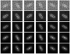 |
Fig. A.1. Data augmentation example for a CLM at redshift z = 0.531 (e.g. within the gravitational potential of M1149). Five HST bands are represented from the top to the bottom (F435, F606, F814, F105, F140). The first column shows the original cut-out, while the three rotations (90°, 180°, 270°) are reported in Cols. 2–4. The two vertical and horizontal flips are shown in the last two columns. |
A.2. Setup of training and test sets
Before the k-fold splitting and the augmentation process, described above, we randomly extracted a small sample of sources (10% of the data set), reserved as validation set during the training phase in order to control the gradual reduction of the learning rate on the plateau of the cost function (Bengio 2012) and an early stopping regularisation process (Prechelt 1997; Raskutti et al. 2011). The data preparation flow is depicted in Fig. A.2: (i) the dataset is composed by multi-bands images; (ii) a fraction of sources (10%) is extracted as validation set; (iii) the remaining samples are split into k = 10 folds without overlapping; (iv) for each of them, a fraction (15%) of samples is augmented through cut-out rotations and flips; (v) the training sets are built by concatenating k − 1 folds (composed by the original images and the artefacts) and the learning is evaluated on the kth fold (without artefacts), acting as blind test; (vi) finally, the model performances are evaluated on the whole training set, obtained by stacking all its (test) folds.
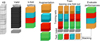 |
Fig. A.2. Data preparation flow: from the whole dataset (i.e. the knowledge base) a validation set is extracted. The rest of the dataset is split through a k-fold partitioning process (in this image, we simplified the figure assuming k = 4 folds, while in reality we used k = 10). The training samples are then arranged, by permuting the involved augmented folds, while the test samples dof not include the artefact images generated by the augmentation process. These sets are finally stacked in order to evaluate the global training performances. |
A.3. Statistical evaluation of performance
In order to assess the model classification performances, we chose the following statistical estimators: “average efficiency” (among all classes, abbreviated as “AE”), “purity” (also know as “positive predictive value” or “precision”, abbreviated as “pur”), “completeness-” (also known as “true positive rate” or “recall”, abbreviated as “comp”), and F1-score (a measure of the combination of purity and completeness, abbreviated as “F1”).
In a binary confusion matrix, as in the example shown in Table A.1, columns indicate the class objects as predicted by the classifier, while rows refer to the true objects per class. The main diagonal terms contain the number of correctly classified objects for each class, while the terms FP and FN report the amount of, respectively, false positives and false negatives. Therefore, the derived estimators are computed as:
Generic confusion matrix for a binary classification problem.
The AE is the ratio between the sum of the correctly classified objects (for all the involved classes) and the total amount of objects; it describes an average evaluation weighted on all involved classes. The “purity” of a class is the ratio between the correctly classified objects and the sum of all objects assigned to that class (i.e. the predicted membership); it measures the precision of the classification. The “completeness” of a class is the ratio between the correctly classified objects and the total amount of objects belonging to that class (i.e. the “true” membership), it estimates the sensitivity of the classification. Finally, the F1-score is the harmonic average between purity and completeness. By definition, the dual quantity of purity is the “contamination”, a measure which indicates the amount of misclassified objects for each class.
Moreover, from the probability vector (i.e. the set of values stating the probability that an input belongs to a certain class), it is possible to extract another useful estimator, the receiver operating characteristic (ROC) curve. It is a diagram in which the true positive rate is plotted versus the false positive rate by varying a membership probability threshold (see Fig. 6). The overall score is measured by the area under the ROC curve (AUC), where an area of 1 represents a perfect classification, while an area of 0.5 indicates a useless result (akin to a toss of a coin).
Appendix B: Convolution neural networks
In this appendix, CNNs theory and our specific implementation are briefly described. while a synthetic view of the implemented model is shown in Fig. B.1.
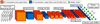 |
Fig. B.1. Streamlined representation of the architecture designed for the CNN model used in this work. Orange and blue items describe two different block operations, respectively: (i) convolution and activation function, (ii) convolution, activation function and pooling. The simultaneous reduction of the square dimensions and their increasing amount intuitively represent the abstraction process typical of a CNN. Green circular units are arranged in order to describe the fully connected (i.e. dense) layers. The dimensions of the feature maps are reported for each pooling operation, together with the number of features extracted by the CNN. |
As any other artificial neural networks, convolution neural networks (CNNs, LeCun et al. 1989) are inspired by biological behaviours. Artificial neurons are arranged in several layers, where each neuron takes as input the signal coming from neurons belonging to the previous layer; such as biological neurons, the variation of the synaptic connection sensibility (with respect to a certain input signal) is correlated to the learning mechanism (Hebb 1949). During the training, these connection sensibilities among layers (i.e. the weights) are adapted through a forward-backward mechanism, at the base of the iterative learning process (Bishop 2006). After training, supervised Machine Learning methods define a non-linear relation between the input and output spaces, which is encoded within the weight matrices.
CNNs represent one of the most widely-used supervised techniques among the Deep Neural Networks (DNN, Goodfellow et al. 2016), whose peculiarity is an ensemble of receptive fields which trigger neuron activity. The receptive field is represented by a small matrix (called as kernel or filter), which connects two consecutive layers through a convolution operation. Similar to the adaptation mechanism imposed by supervised machine learning, the kernels are modified during the training. The peculiarity of such kind of models is the capability to automatically extract meaningful features from images (such as edges and shapes), which become the input vector to any standard ML model that outputs the class of the input image. The idea behind CNN is a convolution-subsampling chain mechanism: deep networks are characterised by tens of layers (in some cases hundreds, as proposed by He et al. 2015 and Xie et al. 2016), where at each depth level, the convolution acts as a filter, emphasising (or suppressing) some properties; while the subsampling (often called pooling) makes sure that only essential information is moved towards the next layer.
CNNs are organised as a hierarchical series of layers, typically based on convolution and pooling operations. Convolution kernel is represented by a 4-D matrix K, where the element Ki, j, k, l is the connection weight between the output unit i and the input unit j, with an offset of k rows and l columns. This kernel is convoluted with the input signal and adapted during the training. Given an input V, whose element Vi, j, k represents an observed data value of the channel i at row j and column k, the neuron activity can be expressed as (Goodfellow 2010):
where c(K, V, s) is the convolution operation between the input V and the kernel K with stride s; b is an addend that acts as bias; p(Z, d) is the pooling operation with down-sampling factor d; f(Z, {a}q) is the activation function characterised by the set of hyper-parameters {a}q. The pooling function reduces the dimension, by replacing the network output at a certain location with a summary statistic of nearby outputs (Goodfellow et al. 2016).
Unlike traditional artificial neural networks (e.g. Multi-Layer Perceptron), where all neurons of two consecutive layers are fully connected among them, the connection among neurons in a CNN is “sparse”, that is, the interaction between neurons belonging to different layers is limited to a small fraction. This reduces the number of operations, the memory requirements and, thus, the computing time. The output layer consists of an ensemble of sub-images with reduced dimensions, called feature maps, each of them represents a feature extracted from the original signal, processed by the net in order to solve the assigned problem.
Another common operation performed during the training of a CNN is the random dropout of weights. This function prevents units from co-adapting, reduces significantly overfitting and gives major improvements over other regularization methods (Srivastava et al. 2014). At the end of the network, the resulting feature maps ensemble is fully connected with one or more hidden layers (also called “dense layers”), the last of which, in turn, is fully connected to the output layer. The net output must have the same shape of the known target: within the supervised learning paradigm, the comparison between output and target induces the kernel adaptations. When the net task is a classification problem (as in this work), the output is a matrix of probabilities, that is, each sample has a membership probability related to any class of the problem. In order to transform floating values into probabilities (i.e. forced to the constraint  ), the activation function of the final dense layer is typically a softmax, which normalises a vector into a probability distribution (Bishop 2006). In order to solve a classification problem, the network learns how to disentangle objects in the train set, minimising a loss function (or cost function). The most common choice for the loss function is the cross-entropy (Goodfellow et al. 2016):
where y is the target and  is the output of the final layer. Thus, during the training, images extracted from the train set are propagated through the network, while weights and biases are adapted along with a backward flow in order to minimise the cost function. To perform such optimization, it is necessary to state the minimization algorithm. The simplest and most used optimiser is the Stochastic Gradient Descendent (Bishop 2006), but in recent years several optimisers have been proposed (e.g. Duchi et al. 2011; Zeiler 2012; Kingma & Ba 2014), which offer a faster convergence to the minimum, avoiding the local dump of the cost function. In this work we chose Adadelta (Zeiler 2012) as optimiser. Furthermore, we included (i) an early stopping regularisation criterion (Prechelt 1997; Raskutti et al. 2011), preventing overfitting; and (ii) a gradual reduction of the learning rate on the plateau of the loss function (as function of epochs, Bengio 2012). Both techniques exploit a validation set, extracted from the train set, used to compute and evaluate the learning efficiency within the training cycles. In our case, to avoid memory loss, the network has been trained with input data batches of size equals to 64 patterns.
The architecture of our VGGNET-like model is reported in Table B.1. It is composed of 47 layers and convolution kernels with a window size of 3 × 3. The max pooling criterion was preferred to the average algorithm, in order to reduce the noise contribution. We set the Leaky version of a Rectified Linear Unit (LeReLU, Maas et al. 2013) as activation function for all the neurons. This type of activation allows (i) a small, non-zero gradient also when the unit is saturated and not active, (ii) a gain of the convergence with the increase of the units, defined as:
VGGNET-like model configuration.
where α is a hyper-parameter set to 0.3.
This network has been implemented through keras (Chollet 2015), with tensorflow (Abadi et al. 2015) as backend system. Both of them are open-source Python libraries, allowing the automatic handling of the Graphic Processing Unit (GPU), achieving a huge gain in terms of computational cost (∼700 see Simard et al. 2005). In this work the experiments were performed with an NVIDIA GPU Titan Xp and an NVIDIA GPU Quadro P5000, requiring ∼30 minutes to complete the training (on a single fold, see Appendix A.2).
Appendix C: Benchmark methods
We compared CNN performances with two techniques based on photometric catalogues: a random forest (RF, Breiman 2001) and a Bayesian Method (briefly described in Grillo et al. 2015).
A Bayesian classifier is a model able to minimise the error probability (Devroye et al. 1996), defined as: L(g) = P[g(X)≠Y], where (X, Y) are pair values ∈ℝd × {1, …, M} (i.e. Y is the ensemble of class labels related to the manifold X), g is a classifier (i.e. a function g : x ∈ X ⊆ ℝd → y ∈ {1, …, M}), L is an application mapping g into probabilities. The minimal probability error is denoted L* = L(g*), that can be written as:
![$$ \begin{aligned} g^* = \underset{g:\mathbb{R} ^d\rightarrow \{1, \dots , M\}}{\mathrm{argmin}} P[g(X)\ne Y] \end{aligned} $$](/articles/aa/full_html/2020/11/aa39083-20/aa39083-20-eq14.gif)
Given a classical linear model  , i = 1, …, n, the method estimates
  in order to minimise a coherent combination of the residuals
  . The implemented method exploits a minimum covariance determinant method (Rousseeuw 1984), which is based on the minimization of the median of squared residuals.
Random forest is a machine learning classifier consisting of a collection of tree-structured classifiers {h(x, θk),k = 1, …} where the {θk} are independent identically distributed random vectors and each tree casts a unit vote for the most popular class at input x. The generalisation error for this algorithm depends on the strength of single trees and from their correlations through the raw margin functions. To improve the model accuracy by keeping trees strength, the correlation between trees is decreased and bagging with a random selection of features is adopted. Bagging, or bootstrap aggregating, is a method designed to improve the stability and accuracy of machine learning algorithms. It also reduces variance and helps to avoid overfitting. In this work, we used the RF provided by Scikit-Learn python library (Pedregosa et al. 2011).
Appendix D: Technical descriptions of our performed experiments
In this appendix, we report tables and figures describing in detail the analysis performed for each experiment.
D.1. EXP1
With this experiment, we evaluated the CNN capabilities to identify CLMs at different cluster redshifts, zcluster ∈ (0.2, 0.6), using different HST band combinations (see Sects. 2 and 4.1). Furthermore, in this experiment, we studied the dependence on redshift and on the number of spectroscopic sources involved in the training. The results related to this experiment have been summarised in Sect. 4.1.
In Table D.1, we report the results achieved globally by CNN, that is, by combining the available clusters (see also Fig. 4), while Table D.2 outlines the performances for each involved cluster, varying the band combinations. The experiment has been carried out with the k-fold approach, stacking sources in the FoV of 13 (15 only for the mixed* configuration) clusters, ensuring that the k-est fold is populated by objects extracted from each involved cluster, proportionally to the number of available spectroscopic sources, that is, providing adequate coverage of the training set respect to the test set.
CNN percentage performances in the EXP1 experiment.
CNN percentage performances evaluated for each cluster and for each band configuration related to the EXP1 experiment.
The comparison between the band configurations is also shown in Fig. D.1, in which performances and their fluctuations are displayed as function of the involved number of samples. For each configuration, we split the knowledge space into ten disjointed subsets, which have been progressively merged in order to build a dataset with which CNN has been trained and tested, always using the k-fold approach.
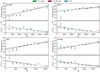 |
Fig. D.1. Comparison among the four band configurations (see Sect. 2), in terms of F1 score and average efficiency (AE) percentages (top panels), together with their square root of variances (bottom panels), as the number of spectroscopic sources in the training set increases (EXP1). In all panels, the linear best-fit trends are displayed as dashed lines. Due to the k-fold approach, performances have been averaged over the 10 folds, i.e. the x-axis shows the dimension of the training set, thus, the k-est fold used as test set has a size of N/9. |
In order to analyse the dependence on redshift, we split the CLM redshift range into five equally populated bins and, to complete the knowledge space, with extracted without repetitions from the NCLM population an appropriate number of objects. The network has been trained within each ensemble adopting the k-fold approach, using only the mixed* band combination. The result is graphically shown in Fig. 5 and it is stored in Table D.3, in which, we have specified the fluctuation of estimators as an error estimated on the ten folds.
Statistical estimators measured in each redshift bin for the EXP1a experiment.
D.2. EXP2
In this experiment, we explored the limits of the CNN in terms of its classification efficiency. With this aim, we excluded three clusters from the training sample, respectively, A370 (z = 0.375), MS2137 (z = 0.316) and M0329 (z = 0.450), which were considered as the blind test set. Such experiment is particularly suitable to evaluate the model capability to predict the cluster membership of sources extracted from clusters unused during training. Furthermore, in this experiment, we varied the training configuration based on three redshift ranges centered on A370 cluster redshift (named as narrow, intermediate and large, see Sect. 4.2 and Fig. 3), exploiting the mixed* band configuration. This experiment has been described in Sect. 4.2. Table D.4 outlines the results achieved on the three configurations together with Fig. 6. As second step, we analysed the CNN classification capabilities by separating, respectively, brighter from fainter (EXP2a), and redder from bluer objects (EXP2b). Concerning the magnitude threshold, we split the CLM F814 distribution into two equal-sized sets (F814 limits are 22.0 mag, 21.7 mag, and 21.6 mag for, respectively, A370, M0329 and MS2137). Regarding the colour split, we exploited the correlation between the Balmer break and the differential colour, as shown in Girardi et al. (2015): (F814 − F160)diff = (F814 − F160Wobs − CM(F814), that is, the difference between the observed colour and the one of the colour-magnitude (CM) relation at a given magnitude. For each cluster, we fitted the CM sequence using a robust linear regression (Cappellari et al. 2013) involving spectroscopic confirmed members. By applying this kind of correction to the source colour, redder members were centered around zero, while bluer objects have differential colours around −0.2 mag. The differential colour thresholds were −0.160, −0.165, −0.157 mag for, respectively, A370, M0329 and MS2137. For both experiments, we opted for a large ensemble and mixed* band configuration. The results are shown in Table 2.
Percentage performances on a blind test set related to the EXP2 experiment.
D.3. EXP3
This test was devoted to the comparison of CNN performance with two different photometry-based methods, exploiting a random forest classifier (Breiman 2001) and a Bayesian model (Grillo et al. 2015). Both techniques critically use multi-band photometric information, for example, magnitudes and colours. This experiment has been outlined in Sect. 4.3. The Bayesian method has already been applied in order to enlarge the cluster member selection, including galaxies without spectroscopic information, for four clusters: R2248, M0416, M1206, and M1149 (Grillo et al. 2015; Caminha et al. 2016, 2017a; Treu et al. 2016). We compare these methods with our CNN, trained with the mixed* band configuration, constraining the results to these four involved clusters. The comparison is summarised in Table D.5 in term of statistical estimators, whereas, in Fig. 7 and Fig. D.3, it is shown in terms of ROC curves (see Appendix A.3), in Fig. D.2 in terms of commonalities among predictions. Particularly, we also compared performances between CNN and photometric methods by computing the differences: Δestim = estimCNN − max{estimRF, estimBayesian} for estim ∈ [pur, compl, F1, AE], that is, the difference between CNN metrics and the corresponding maximum scores achieved by RF or Bayesian model. All these differences are listed in the last column of Table D.5, together with the average among these Δs for each cluster (rows μΔ).
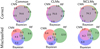 |
Fig. D.2. Venn diagrams reporting the percentages of membership predictions performed by three different methods (CNN, RF, and Bayesian), measured on the common blind test set, obtained by combining the four clusters R2248, M0416, M1206, and M1149 (EXP3). On the columns, the common areas refer to the available shared sources, respectively, 460 CLMs and 519 NCLMs). On the rows, common predictions are split between correct and incorrect classifications. Global commonalities can be derived by summing values on the rows. |
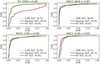 |
Fig. D.3. Comparison between the image-based CNN ant two photometric catalogue-based approaches, RF and Bayesian method (EXP3) in term of ROC curves for the four clusters: R2248 (top-left panel), M0416 (top-right panel), M1206 (bottom left panel), M1149 (bottom right panel). |
Comparison between our image-based CNN model and two different photometric catalogue-based approaches, referred to the EXP3 experiment.
An additional comparison of the three methods based on common membership predictions (see Fig. D.2), is discussed in Sect. 4.3.
All Tables
Comparison among CNN performances considering the whole sample (Col. 2) and by removing sources with F814 ≥ 25 and (F606 − F814)diff < −0.5 (Col. 3).
CNN percentage performances evaluated for each cluster and for each band configuration related to the EXP1 experiment.
Statistical estimators measured in each redshift bin for the EXP1a experiment.
Comparison between our image-based CNN model and two different photometric catalogue-based approaches, referred to the EXP3 experiment.
All Figures
|
Fig. 1. Colour-composite images of the 15 clusters included in our analysis, obtained by combining HST bands from optical to near IR. The images are squared cut-outs, ∼130″ across, centred on the cluster core. |
| In the text | |
|
Fig. 2. Examples of cut-outs of cluster members extracted from HST images (F435, F606, F814, F105, F140 bands), corresponding to five clusters (from top to bottom): A383 (z = 0.188), R2248 (z = 0.346), M0416 (z = 0.397), M1206 (z = 0.439), M1149 (z = 0.542). All the cut-outs are 4 arcsec across. |
| In the text | |
|
Fig. 3. Redshift distribution of 1629 spectroscopic members used for the EXP2 configuration. The three clusters A370 (z = 0.375, 224 CLMs), MS2137 (z = 0.316, 45 CLMs) and M0329 (z = 0.450, 74 CLMs) are used as blind test set. |
| In the text | |
|
Fig. 4. Performance percentages of the CNN in the EXP1 experiment with the four band configurations (see Sect. 2) in terms of the statistical estimators described in Appendix A.3. |
| In the text | |
|
Fig. 5. Percentages of CNN classification results for the four statistical estimators, measured as a function of CLM redshift range (EXP1). The top panel describes their fluctuation in each bin, with the boxes delimiting the 25th and 75th percentiles (first and third quartile) and error bars enclosing the maximum point variations. The bottom panel shows the same metrics globally evaluated in each redshift bin, together with the best-fit lines. |
| In the text | |
|
Fig. 6. Summary of the EXP2 experiment. The statistical performances for the three clusters (A370, M0329 and MS2137) are reported in each row, while results for the three training configurations (i.e. narrow, intermediate and large) are organised by column. The global performances achieved by stacking together the three clusters are reported in the bottom row. For each test set, we display the ROC curves (grey lines refer to the performances achieved by any training fold, while the main trend is emphasised in red, together with its AUC score); the box plots represent the fluctuation of measured estimators related to the CLMs, together with the average efficiency measured for both classes. As in Fig. 5, such boxes delimit the 25th and 75th percentiles, while error bars enclose the maximum point variations. |
| In the text | |
|
Fig. 7. Comparison among the image-based CNN and two photometric catalogue-based approaches, namely, a random forest and Bayesian method (EXP3), by combining results from the four clusters (R2248, M0416, M1206, M1149). Upper panel shows the ROC curves for the three methods with measured Area Under the Curve (AUC). The middle panel reports the trends of purity and completeness as a function of the probability thresholds used to obtain the ROC curves. In the three diagrams, we mark the intersection between such curves, i.e. the probability for which completeness and purity are equal. Bottom panel shows the differences between the three methods based on the statistical estimators described in Appendix A.3. |
| In the text | |
|
Fig. 8. CNN member selection (marked with open magenta squares) obtained with the run set, together with the spectroscopic CLMs (marked with open green squares), in the core of the four clusters R2248 (z = 0.346), M0416 (z = 0.397), M1206 (z = 0.439) and M1149 (z = 0.542). All images are 130 arcsec across. |
| In the text | |
|
Fig. 9. CNN membership prediction (run) together with spectroscopic sources, represented as (i) CLMs distribution of F814 magnitudes (first row), (ii) differential colour – magnitude sequence for both CLMs and NCLMs. Spectroscopic CLMs are shown in green, candidate members in purple, spectroscopic NCLMs with blue squares and candidate NCLMs with open cyan circle. We only plot CNN cluster members with F814 ≤ 25 mag. The grey region within the CM diagrams limits the area corresponding to ±1σ from the median (dashed horizontal line) of (F606 − F814)diff. |
| In the text | |
|
Fig. 10. Ensemble of object cut-outs with a size of 64 pixels (∼4″), corresponding to some specific CNN predictions in the clusters R2248 (first three rows) and M0416 (last two rows). The True Positives (TPs), i.e. the CLMs correctly identified, are shown on first and fourth row with green boxes, while False Positive and False Negative (FPs and FNs) are shown on the second, third and fifth row, framed by red and blue boxes, respectively. The images were obtained by combining five HST bands: F435, F606, F814, F105, F140. The figure shows sources in the F814 band with a magnitude F814 ≤ 25 mag. TPs are shown together with their spectroscopic redshift, while FNs together with their cluster rest-frame velocity separation. For convenience, in the case of FPs, their cluster velocity separations are quoted when within ±9000 km s−1, otherwise their redshift is shown. |
| In the text | |
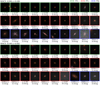 |
Fig. 11. Same of Fig. 10 for the cluster M1206 (first three rows) and M1149 (last three rows). |
| In the text | |
|
Fig. 12. Logarithmic distribution of the contamination index for true positives (TPs, green), true negatives (cyan), false positives (red), and false negatives (blue). The distribution includes all available clusters. |
| In the text | |
|
Fig. 13. Magnitude (left panel) and colour (right panel) logarithmic distributions of FPs (red) and FNs (blue), overlapped to the CLM (green) and NCLM distributions, for the fifteen clusters (stacked) included in our study. The number of objects for each plotted distribution is quoted in brackets in the legend. The differential colour (F606 − F814)diff is obtained by applying the correction for the mean colour-magnitude relation for each cluster. Table 3 outlines such results. |
| In the text | |
|
Fig. 14. Colour-magnitude relation for the CLMs (green squares), with the overlapped distributions of FPs (red crosses), FNs (blue crosses) and NCLMs (grey circles), for the sample of fifteen clusters (stacked). The yellow contour delimits the red-sequence at 1σ confidence level. Colours reported on the y-axis are corrected for the mean red-sequence of each cluster (see Sect. 4). |
| In the text | |
|
Fig. 15. Cumulative (left) and differential (right) projected number of CLM for the four clusters (R2248, M0416, M1206, and M1149), including spectroscopic CLMs and candidate members identified by CNN (limited to F814 ≤ 25 mag). The areas correspond to the 68% confidence level regions. All profiles are normalised by the number N0 of members with R < 0.15 R200 in all clusters. The number of spectroscopic, CNN-identified members (“run”), and N0 values are quoted in the left panel. The adopted values of R200 are quoted in the right panel, the computed values of N0 are quoted in the left panel, together with the corresponding numbers of spectroscopic and “run” members. The dashed line in the right panel corresponds to R = 0.15 R200. |
| In the text | |
|
Fig. A.1. Data augmentation example for a CLM at redshift z = 0.531 (e.g. within the gravitational potential of M1149). Five HST bands are represented from the top to the bottom (F435, F606, F814, F105, F140). The first column shows the original cut-out, while the three rotations (90°, 180°, 270°) are reported in Cols. 2–4. The two vertical and horizontal flips are shown in the last two columns. |
| In the text | |
|
Fig. A.2. Data preparation flow: from the whole dataset (i.e. the knowledge base) a validation set is extracted. The rest of the dataset is split through a k-fold partitioning process (in this image, we simplified the figure assuming k = 4 folds, while in reality we used k = 10). The training samples are then arranged, by permuting the involved augmented folds, while the test samples dof not include the artefact images generated by the augmentation process. These sets are finally stacked in order to evaluate the global training performances. |
| In the text | |
|
Fig. B.1. Streamlined representation of the architecture designed for the CNN model used in this work. Orange and blue items describe two different block operations, respectively: (i) convolution and activation function, (ii) convolution, activation function and pooling. The simultaneous reduction of the square dimensions and their increasing amount intuitively represent the abstraction process typical of a CNN. Green circular units are arranged in order to describe the fully connected (i.e. dense) layers. The dimensions of the feature maps are reported for each pooling operation, together with the number of features extracted by the CNN. |
| In the text | |
|
Fig. D.1. Comparison among the four band configurations (see Sect. 2), in terms of F1 score and average efficiency (AE) percentages (top panels), together with their square root of variances (bottom panels), as the number of spectroscopic sources in the training set increases (EXP1). In all panels, the linear best-fit trends are displayed as dashed lines. Due to the k-fold approach, performances have been averaged over the 10 folds, i.e. the x-axis shows the dimension of the training set, thus, the k-est fold used as test set has a size of N/9. |
| In the text | |
|
Fig. D.2. Venn diagrams reporting the percentages of membership predictions performed by three different methods (CNN, RF, and Bayesian), measured on the common blind test set, obtained by combining the four clusters R2248, M0416, M1206, and M1149 (EXP3). On the columns, the common areas refer to the available shared sources, respectively, 460 CLMs and 519 NCLMs). On the rows, common predictions are split between correct and incorrect classifications. Global commonalities can be derived by summing values on the rows. |
| In the text | |
|
Fig. D.3. Comparison between the image-based CNN ant two photometric catalogue-based approaches, RF and Bayesian method (EXP3) in term of ROC curves for the four clusters: R2248 (top-left panel), M0416 (top-right panel), M1206 (bottom left panel), M1149 (bottom right panel). |
| In the text | |
Current usage metrics show cumulative count of Article Views (full-text article views including HTML views, PDF and ePub downloads, according to the available data) and Abstracts Views on Vision4Press platform.
Data correspond to usage on the plateform after 2015. The current usage metrics is available 48-96 hours after online publication and is updated daily on week days.
Initial download of the metrics may take a while.