| Issue |
A&A
Volume 698, June 2025
|
|
|---|---|---|
| Article Number | A272 | |
| Number of page(s) | 14 | |
| Section | Extragalactic astronomy | |
| DOI | https://doi.org/10.1051/0004-6361/202554495 | |
| Published online | 19 June 2025 | |
Virial quantities of galaxy clusters from extrapolating strong-lensing mass profiles
1
Dipartimento di Fisica, Università degli Studi di Milano, Via Celoria 16, I-20133
Milano, Italy
2
INAF – IASF Milano, Via A. Corti 12, I-20133
Milano, Italy
3
INAF – OAS, Osservatorio di Astrofisica e Scienza dello Spazio di Bologna, Via Gobetti 93/3, I-40129
Bologna, Italy
4
INFN – Sezione di Bologna, Viale Berti Pichat 6/2, I-40127
Bologna, Italy
⋆ Corresponding author: enrico.maraboli@unimi.it
Received:
12
March
2025
Accepted:
5
May
2025
We study the radial total mass profiles of nine massive galaxy clusters (M200c > 5 × 10¹⁴ M⊙) in the redshift range 0.2 < z < 0.9. These clusters were observed as part of the CLASH, HFF, BUFFALO, and CLASH-VLT programs, which provided high-quality photometric and spectroscopic data. Additional high-resolution spectroscopic data were obtained with the integral-field spectrograph MUSE at the Very Large Telescope. Our research takes advantage of strong-lensing analyses that rely on deep panchromatic and spectroscopic measurements. From these data, we measure the projected total mass profiles of each galaxy cluster in our sample. We fit these mass profiles with simple one-component spherically symmetric mass models including the Navarro–Frenk–White (NFW) nonsingular isothermal sphere, dual pseudo-isothermal ellipsoidal, a beta model, and Hernquist profiles. We performed a Bayesian analysis to sample the posterior probability distributions of the free parameters of the models. We find that the NFW, Hernquist, and beta models are the most suitable profiles for fitting the measured projected total mass profiles of the clusters. Moreover, we tested the robustness of our results by changing the region in which we performed the fits: We slightly modified the center of the projected mass profiles and the radial range of the region. We employed the results obtained with the Hernquist profile to compare our total mass estimates (MHtot = MH(r→+∞)) with the M200c values from weak-lensing studies. Through this analysis, we found scaling relations between MHtot and M200c and a value of the scale radius, rS, and R200c. Interestingly, we also found that the M200c values we obtained by extrapolating the total mass profiles we fit are very close to the weak-lensing results. This feature can be exploited in future studies of clusters and cosmology because it provides an easy way to infer the virial masses of clusters.
Key words: galaxies: clusters: general / cosmology: observations
© The Authors 2025
 Open Access article, published by EDP Sciences, under the terms of the Creative Commons Attribution License (https://creativecommons.org/licenses/by/4.0), which permits unrestricted use, distribution, and reproduction in any medium, provided the original work is properly cited.
This article is published in open access under the Subscribe to Open model. Subscribe to A&A to support open access publication.
1. Introduction
Galaxy clusters play a crucial role in astrophysics and cosmology. They are some of the most interesting physics laboratories for studying the evolution and current state of the Universe. They have therefore been the targets of many recent observational campaigns that were carried out by facilities such as the Hubble Space Telescope (HST), the Spitzer Space Telescope (SST), the Röntgensatellit (ROSAT), and the James Webb Space Telescope (JWST) (e.g., Postman et al. 2012; Mann & Ebeling 2012; Lotz et al. 2017; Bezanson et al. 2024; Treu et al. 2022). In addition to these space-based observations, ground-based complementary follow-up programs have been set up to complete the photometric and spectroscopic datasets (see, e.g., Rosati et al. 2014). The general purpose of this intense data collection is to provide the most accurate description of galaxy clusters by creating a detailed multiwavelength view of these structures on a wide range of scales. One of the most interesting features of galaxy clusters is their mass composition. This includes not only the stellar component (≤5% of total mass), but also the dark matter (DM; 80%–85% of total mass) and hot intracluster gas (also known as the intracluster medium; ICM. This constitutes 10%–15% of the total mass). The mass components of the galaxy clusters are often in a dynamical equilibrium status, which makes them very sensitive and effective cosmological probes (Kravtsov & Borgani 2012). By studying the matter composition of the galaxy cluster and the distribution of the different mass components, we can provide a fair test of the currently accepted cosmological model by testing the dark matter accretion theories or the hierarchical paradigm growth of large-scale structures, and we can constrain the normalized value of the baryonic density of the Universe, ΩB (Bahcall & Kulier 2014). Moreover, the cosmological simulations parameters can be tuned better when they are based on accurate studies of the mass composition to provide further checks and insights into current cosmological theories (Huss et al. 1999).
We study the total mass distribution of galaxy clusters starting from the results obtained by strong lensing (SL). To do this, we exploit the new results from the campaigns described above. We analyze nine massive (total mass M200c > 5 × 10¹⁴ M⊙) galaxy clusters in the redshift range 0.2 < z < 0.9 by fitting the projected radial mass profiles of the total mass with a set of single-component spherical models. We base our work on robust mass measurements obtained from the most recent SL studies (Caminha et al. 2016, 2017a,b; Bonamigo et al. 2017, 2018; Bergamini et al. 2019; Caminha et al. 2019, 2023; Bergamini et al. 2023), from which we derive the cumulative total mass profiles that we studied. The main purpose of this paper is to investigate whether the total mass profiles of our sample of galaxy clusters can be described by one (or more) spherically symmetric parametric models. We also test whether any of the models that reproduce the mass profiles better is related to a finite value of the total mass for r → +∞. When this occurs, we search for a relation between the total mass of the galaxy clusters obtained from our models and the respective values of M200c1 derived from the weak-lensing analysis (e.g., Umetsu et al. 2018).
The paper is organized as follows. In Section 2 we present the galaxy clusters sample, the dataset, and the derived total projected mass profiles from previously published strong-lensing galaxy cluster studies. In Section 3 we present all the models we employed to reconstruct the projected mass profiles and the methods we used to perform the numerical fits. In Section 4 we present the results of the numerical fits of the total mass profiles, and we discuss the performance of our models. In Section 5 we present the relation that we find between the total masses from our models and the M200c values from the literature. In Section 6 we discuss our results and the interplay between our models and the adopted hypotheses. Throughout the paper, we assume a flat ΛCDM cosmological model, in which the Hubble constant value is H0 = 70 km s−1 Mpc−1, and the total matter density value is Ωm = 0.3.
2. Data sample
We studied the nine galaxy clusters listed in Table 1: RX J2129.7+0005 (namely RXJ2129), Abell 2744 (A2744), RXC J2248.7−4431 (AS1063), MACS J1931.8−2635 (M1931), MACS J0416.1−2403 (M0416), MACS J1206.2−0847 (M1206), MACS J0329.7−0211 (M0329), MACS J2129.4−0741 (M2129), and ACT-CL J0102−4915 (ACT0102, or El Gordo). These are massive galaxy clusters with M200c > 5 × 10¹⁴ M⊙, and they span a wide redshift range (0.2 < z < 0.9). They are quite regular virialized clusters that are observed by different photometric and spectroscopic observational campaigns. We report the details of these campaigns in the next sections.
List of the galaxy clusters with relevant information for the strong-lensing analyses.
The nine galaxy clusters were selected to have high-quality and homogeneous data that were the basis for the accurate strong-lensing models in the reference papers. The high-quality data enabled us to measure the total mass values and cumulative mass profiles of the clusters, which we used here.
2.1. Photometric and spectroscopic data in SL models
The projected total mass measurements of the cluster, as we show below, come from different studies that mainly relied on the observations made by the Cluster Lensing And Supernova survey with the HST (CLASH; Postman et al. 2012). All the clusters of our sample except for A2744 and ACT0102 were targeted by CLASH, and this program is the main photometric source for them. In addition to CLASH, HST took images of M0416, A2744, and AS1063 within the Hubble Frontier Fields (HFF; Lotz et al. 2017) program. This significantly augmented their photometric datasets by adding deeper exposures in seven filters (F435W, F606W, F814W, F105W, F125W, F140W, and F160W).
The photometry of A2744 is composite, and it takes advantage of many different sources in addition to the HFF program, for example, from the Beyond Ultra-deep Frontier Fields And Legacy Observations (BUFFALO; Steinhardt et al. 2020) program and from the recent observations of the GLASS-JWST (Treu et al. 2022) program. The complete list of the photometry sources for A2744 can be found in Section 2.1 of Bergamini et al. (2023).
For ACT0102, the photometric observations employed by Caminha et al. (2023) were provided by the Reionization Lensing Cluster Survey (RELICS; Coe et al. 2019) program.
Most of the spectroscopic data for the galaxy clusters in this paper were taken from the Multi Unit Spectroscopic Explorer (MUSE; Bacon et al. 2010) at the Very Large Telescope (VLT). MUSE observations are available for every galaxy cluster we studied, and they have been exploited in the strong-lensing analyses by Caminha et al. (2019, 2023) and Bergamini et al. (2019, 2023) (see these papers for a detailed description of each MUSE pointing). The MUSE exposure time for each galaxy cluster in the sample is 2.45 hours at least, and this time was one of the determining factors for the choice of our galaxy cluster sample.
The other main spectroscopic data source for the galaxy clusters in this paper was the CLASH-VLT program (Rosati et al. 2014), which relied on the VIsual Multi-Object Spectrograph (VIMOS; Le Fèvre et al. 2003). This program targeted all the galaxy clusters in our sample, except for A2744 and ACT0102.
Although A2744 is not part of CLASH-VLT, its spectroscopic dataset includes other VIMOS observations (Braglia et al. 2009) in addition to the data from MUSE: the Grism Lens-Amplified Survey from Space (GLASS; Treu et al. 2015) and the AAOmega multi-object spectrograph (Owers et al. 2011) (see Bergamini et al. 2023 for details). The SL analysis by Caminha et al. (2023) of ACT0102 instead entirely relied on the MUSE observations.
2.2. Strong-lensing data
The cluster-projected total mass profiles come from homogeneous strong-lensing analyses in our sample. In particular, we extracted the cumulative total mass profiles from the mass models reconstructed by Caminha et al. (2019) for M0329, RXJ2129, M1931, and M2129; by Bergamini et al. (2019) for AS1063, M0416, and M1206; by Caminha et al. (2023) for ACT0102, and by Bergamini et al. (2023) for A2744. The authors employed the robust photometric and spectroscopic information described above either to build new strong-lensing models, for example, Bergamini et al. (2023), or to enhance some existing models by adding new observations. As an example, in the analysis of AS1063, M0416, and M1206, Bergamini et al. (2019) combined the stellar kinematic information of the cluster members with strong-lensing models based on large samples of spectroscopically confirmed multiple images. There, the kinematic measurements provided specific priors for the free parameters of the lens model describing the total mass distribution of the cluster members. This additional effort allowed the authors to improve the previous models implemented by Caminha et al. (2016, 2017a,b) for AS1063, M0416, and M1206, respectively, by reducing some degeneracies among the free parameters.
The total mass distribution of a cluster in parametric lens models is generally divided into a widespread component on the cluster scale, made of one or more DM halos, and a subhalo component on smaller scales that traces the cluster galaxies (Natarajan & Kneib 1997). The cluster-scale mass components are commonly modeled with pseudo-isothermal elliptical mass distributions (PIEMD; Kassiola & Kovner 1993), while the galaxy-scale subhalos are modeled with dual pseudo-isothermal mass density profiles (dPIE; Elíasdóttir et al. 2007). In order to reduce the number of free parameters of the model, it is generally assumed that the parameters of the subhalo population (the central velocity dispersion of the cluster member, σv, gal, and the truncation radius, rcut, gal) follow a scaling relation that is compatible with the so-called tilt of the fundamental plane,
where Lgal is the luminosity of the cluster member, and Lref is the reference luminosity;  and
and  are assumed to be free parameters. The total mass distribution of every galaxy cluster was modeled with the publicly available software lenstool (Kneib et al. 1996; Jullo et al. 2007, 2010). The characteristics of the strong-lensing model are different for each galaxy cluster. In Table 1 we report some relevant information of the SL analysis, such as the number of cluster members included in each lensing model and the number of multiple images employed as observables. In the last column of Table 1, we report the values of the total root mean-square separation between the model-predicted and observed positions of the multiple images (ΔRMS). We note that the median ΔRMS value of the model is < 0.8 arcsec. This feature demonstrates the high quality of the strong-lensing studies on which our paper is based and is also reflected by the very small errors on the projected total mass profiles. These small errors consequently made so that the free parameters of our models have small statistical uncertainties, as we show in Section 4.
For each cluster, we derived the cumulative projected total mass profiles from the corresponding strong-lensing model by considering circular regions with increasing radii on the projected plane of the sky and by measuring the total mass value enclosed within every circle. The clusters AS1063, M1206, RXJ2129, M1931, M0329, and M2129 have a single brightest central galaxy (BCG), and the circular regions are accordingly centered on it. For A2744, we decided to center our profile on the northern BCG of the main clump (called BCG-N in Bergamini et al. 2023). Similarly, we centered the circular regions for M0416 on the northern BCG and for ACT0102 on the southern BCG. In order to test the robustness of our results, we tested for the galaxy clusters A2744, M0416, M0329, and ACT0102 whether the best-fit parameters of the deprojected mass models changed significantly when the center of the circular regions was moved to another point. We fully describe this and the outcomes of these tests in Section 6.3. In Figure 1 the maximum circular regions and circle centers are marked in red.
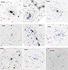 |
Fig. 1. The galaxy clusters of our sample. The background images are from the HST and JWST optical/infrared passbands. The blue circles represent the positions of the multiple images employed in the strong-lensing studies by Caminha et al. (2019, 2023) and Bergamini et al. (2019, 2023). The red circles show the area surrounding the multiple images that we considered for the measurement of the projected total mass profiles. The red crosses indicate the centers of the red circles and the origin point of each projected total mass profile. The green lines represent the radii of the red circles, whose length is shown near them. |
In conclusion, the final dataset for each cluster consisted of ∼100 measurements of its projected cumulative total mass with increasing radial distance (MSL(R) hereafter), accompanied by their intervals at the 68%, 95%, and 99.8% confidence levels.
3. Mass models
The accurate photometric and spectroscopic multiband data listed in the previous section allowed us to inspect the mass structure for each galaxy cluster in the sample in detail. The different mass diagnostics employed by previous works on these clusters, such as strong lensing, weak lensing, galaxy, and hot gas dynamics (see, e.g., Biviano et al. 2013; Bonamigo et al. 2018; Caminha et al. 2019; Sartoris et al. 2020; Bergamini et al. 2023), showed unprecedent details of the total mass structure of these clusters, in particular, in their central regions. In some specific cases (see, e.g., Bonamigo et al. 2017, 2018), it was shown that these structures are composed of a set of smaller substructures. However, we decided to simplify and modeled all the galaxy clusters by assuming one-component spherically-symmetric mass models. As we discuss in Section 6, the symmetry breaking introduced by the substructures does not seem to affect the MSL(R) profiles and their fits significantly.
3.1. Models for the total mass distribution
We tested several mass models to fit the MSL(R) profiles. These were all spherical models with two or thre free parameters. In the following, we present all the parametric mass density profiles, ρ(r), we employed, together with their corresponding three-dimensional cumulative mass profiles, M(r), which are linked through the relation
We indicate with ρ0 and rs (or rC and rT) the values of the characteristic scale mass density and radius. In detail, we considered
-
the Navarro–Frenk–White (Navarro et al. 1997) profile,
-
the nonsingular isothermal sphere (NIS) profile,
-
the dual pseudo-isothermal ellipsiodal (dPIE) profile (Kassiola & Kovner 1993; Elíasdóttir et al. 2007),
-
the Herquist profile (Hernquist 1990),
and
-
the beta profile (e.g., Ettori 2000),
where 2F1 is the hypergeometric function (Gauss 1813), and β is another free parameter in addition to ρ0 and rs.
![$$ \begin{aligned} \rho _{\rm NFW}(r)&=\frac{\rho _{\rm 0}}{\frac{r}{r_{\rm s}}\left(1+\frac{r}{r_{\rm s}}\right)^2} \, ;\nonumber \\ \quad M_{\rm NFW}(r)&= 4\pi \rho _{\rm 0}r_{\rm s}^3\left[\ln {\left(1+\frac{r}{r_{\rm s}}\right)}- \frac{r}{r+r_{\rm s}}\right], \end{aligned} $$](/articles/aa/full_html/2025/06/aa54495-25/aa54495-25-eq7.gif)
![$$ \begin{aligned} \rho _{\rm NIS}(r) = \frac{\rho _{\rm 0}}{4\pi } \frac{1}{1+\frac{r^2}{r_{\rm s}^2}} \ ; \ M_{\rm NIS}(r) = \rho _{\rm 0}r_{\rm s}^3 \left[\frac{r}{r_{\rm s}}-\mathrm{arctan}\left(\frac{r}{r_{\rm s}}\right)\right], \end{aligned} $$](/articles/aa/full_html/2025/06/aa54495-25/aa54495-25-eq8.gif)
![$$ \begin{aligned} \rho _{\rm \beta }(r) = \frac{\rho _{\rm 0}}{4\pi } \frac{1}{\left(1+\frac{r^2}{r_{\rm s}^2}\right)^{3 \beta /2}} \ ; \ M_{\rm \beta }(r) = \frac{1}{3} \rho _{\rm 0}r^3 \, _2F_1 \left[\frac{3}{2},\frac{3\beta }{2}, \frac{5}{2}, -\frac{r^2}{r_{\rm s}^2}\right], \end{aligned} $$](/articles/aa/full_html/2025/06/aa54495-25/aa54495-25-eq11.gif)
3.2. Projection and MCMC fitting
To fit the cluster cumulative projected total mass profiles, we adopted the following formula for the cumulative two-dimensional mass, M(R), which was derived from the projection of the total mass density profile,
where M(r) is the three-dimensional mass profile (see Equation (2)), and
is the surface mass density. We note that we indicate the projected two-dimensional radius and the three-dimensional radius with R and r , respectively.
In order to perform the numerical fits of the MSL(R) profiles, we adopted a Bayesian approach to optimize the free parameters. Specifically, we used the publicly available Python library emcee (Foreman-Mackey et al. 2013) to sample the posterior distributions of the model free parameters. The values presented as results in the next section correspond to the 50th percentile (the median) and to the 16th and 84th percentiles (the 1σ confidence level errors) of the posterior distributions. Henceforth, we report the median values of the free parameters for each total mass model, and we consequently plot the corresponding profiles.
4. Results
In Figure 2 we show the cumulative projected total mass profiles for each cluster in the sample and the corresponding errors together with the best-fitting profiles for each model and their respective uncertainties. The reported error bars and shadowed regions were computed with a two-step method. The first step consisted of randomly selecting 100 sets of parameter values from the Monte Carlo Markov chains, and to generate the corresponding total mass profiles with them. The second step was to extract at each projected radius R the 16th and the 84th percentiles of the previously generated 100 total mass values and to identify them as the confidence boundaries.
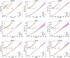 |
Fig. 2. Cumulative projected total mass profiles for the nine clusters in the sample. The red dots show the measured values with their corresponding errors (1σ error bars), and the solid lines represent the best fits of the MSL(R) profiles of each mass model (NFW, NIS, Hernquist, and beta model). The shaded regions represent the 1σ (68%) confidence regions. Each dashed rectangle is zoomed-in the upper left corner of each plot. |
We fit the measured MSL(R) profiles with all the mass models we presented in Section 3.1: Figure 2 demonstrates that different mass profiles reproduce the SL total mass measurements equally well. When we focus on the central cluster regions, the dPIE and NIS models produce very similar results. This behavior can be explained by noting that the sizes of the investigated radial regions are small compared to the scale of a possible truncation radius rT and that the dPIE profile reduces to an NIS profile when rT ≫ r, as in our case. Henceforth, we only report the results for the NIS model because they are the same as those for the dPIE model. In Figure 3 we show the relative differences ΔSL, defined as
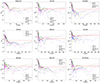 |
Fig. 3. Absolute values of the relative differences between the measured and modeled cumulative projected total mass profiles rescaled to the measured profiles (ΔSL; see Equation (10)) for each galaxy cluster. The horizontal red line in each plot represents the 5% threshold. |
where  is the 2D projection (see Equation (8)) of the mass models listed in Section 3.1. The ΔSL values are almost always low, except in the very central regions up to 20–25 kpc. Additionally, we report in Table 2 the values of the reduced χ2 for the different models. These values are significantly higher than one for some of the galaxy clusters in the sample. This is due to the simplified (circular one-component) total mass parameterization that we adopted. As explained in Section 2.2, the very small errors (barely visible in Figure 2) on the measured projected total mass values result in strongly peaked probability distributions and in accordingly small uncertainties for the free parameter values of each model. Nevertheless, the small relative difference between the models and measurements (see Figure 3) demonstrates that our models are good global probes of the measured total mass profiles we studied. In the following subsections, we discuss the results of our fits and the performances of our mass models for each galaxy cluster in detail.
Values of the reduced χ2 for each mass profile fit to the sample of galaxy clusters
4.1. M0416, M1206, and ACT0102
The galaxy clusters M0416, M1206, and ACT0102 are best represented by a NFW mass profile. Interestingly, these three clusters share another common feature: They were all proven to be merging clusters (e.g., Jee et al. 2014; Balestra et al. 2016). Figure 2 shows that while all models reproduce the MSL(R) profiles well for small radii, the NFW model fits the outer regions of the three galaxy clusters better. This behavior is confirmed by the reduced χ2 values reported in Table 2. We also note that the results obtained from the fits of the Hernquist profile are almost as compatible with the data as those of the NFW model. This demonstrates that this profile reconstructs the total mass profiles of the clusters equally well.
4.2. AS1063, M1931, and M2129
The model that describes the total mass profile of AS1063, M1931, and M2129, best is the Hernquist profile as we show in Table 2. For these three galaxy clusters, the difference between the proposed models is not clearly visible in the plots in Figure 2. Although the Hernquist model is best suited for these clusters, the small difference between the Hernquist and NFW reduced χ2 values means that these two models fit the measurements equally well.
We note an interesting feature in the measured total mass profile of M1931: a kink at very small radii, smaller than 5 kpc. This peculiar characteristic arises from the underlying model of the DM halo, which was obtained in the strong-lensing analysis (see Section 2.2). For most of the galaxy clusters, the reconstructed DM mass distribution is approximately flat in the center, but the main DM halo of M1931 (similarly to those of AS1063 and M2129) has a particularly small core radius, unlike AS1063 and M2129. This creates the small difference between the DM halo and the BCG centers, and in the case of M1931, it is particularly well visible.
4.3. RXJ2129, A2744, and M0329
For RXJ2129, A2744, and M0329, the best-fit of their MSL(R) is obtained with the beta model. The strong agreement between this model and the measured total mass profile for M0329 is clearly visible in Figure 2. Even though it is not evident from the figures, the beta profile is also the best-fitting model for RXJ2129 and A2744, as shown in Table 2. We note that the other available models for these three clusters are not as competitive with the best model as they were in the previous cases. Moreover, similarly to M1931, the projected mass profile of RXJ2129 presents a kink at radii smaller than 5–6 kpc.
5. Virial mass relation
We note that the Hernquist profile alone of the adopted mass profiles listed in Section 3.1 has a finite value of M(r) for r → +∞. We call this quantity  , which from Equation (6) is
By using the inferred values and uncertainties of ρ0 and rs, we measured the values of  for each cluster in the sample, and we compared them with the values of M200c obtained from independent weak-lensing (WL) analyses. Specifically, as shown in Table 1, the available M200c values were measured by Umetsu et al. (2018)2 for AS1063, M0416, M1206, RXJ2129, M1931, and M0329, by Medezinski et al. (2016) for A2744, and by Jee et al. (2014) for ACT0102. At the time of writing, no measurements for the M200c value of M2129 were available. We therefore excluded this galaxy cluster from the followinganalyses.
In Figure 4 we plot  as a function of M200c for the different galaxy clusters. Moreover, we selected a subsample of galaxy clusters in which we only included the most regular clusters (namely RXJ2129, AS1063, M1931, M1206, M0329, and M2129) from the original sample. Since our study is based on strong-lensing models, we considered as regular clusters those that were modeled with a single main dark matter halo and showed no evident substructures. For these six clusters, the hypothesis of a spherical symmetry is more valid, and we expected to obtain a
  versus M200c scaling relation that is more precise for this sample than for the whole sample. We fit the
  and M200c values of this smaller set of galaxy clusters with a linear function and a power law. We report in Table 4 the median values and 1σ confidence level errors of their free parameters, together with the corresponding reduced χ2 values. Although there is some scatter, these scaling relations can provide a fair estimate of M200c by analyzing only the innermost regions of a regular galaxy cluster.
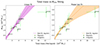 |
Fig. 4. Scaling relation between the total mass from the Hernquist profile, |

Furthermore, we searched for a possible linear scaling relation between the values of the characteristic radius of the Hernquist model (rS; see Table 3) and those of R200c. We computed the R200c values and their errors starting from the M200c measurements reported in Table 1 by assuming the cosmological model described at the end of Section 1. In Figure 5 we plot the relation between rS and R200c. We note that the difference between the two galaxy cluster subsamples is even clearer here than in the previous case. Moreover, the R200c value for ACT0102 is not the highest of the cluster sample, as might be expected because it has the highest M200c value. This is due to the significantly higher critical cosmic mass density value at the ACT0102 redshift (0.87), which is ∼335 M⊙/kpc3, which is different from the ≲200 M⊙/kpc3 for the other galaxy clusters.
Median values and 1σ confidence level errors of the parameters for each total mass model for each galaxy cluster.
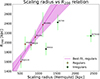 |
Fig. 5. Relation between the fitted scale radii of the Hernquist profile, rs, and the R200c values obtained from the available values of M200c. The solid line shows the linear best fit, and its corresponding 1σ uncertainty is represented by the shaded zone. |
We list the parameter values of this fit and the reduced χ2 value in Table 4. In particular, we note that when we blindly apply the scaling law found from the regulars to the large-scale radii of A2744, M0416, and ACT0102 (the less regular clusters), we find values of R200c that are higher than those measured from WL. This behavior can be explained by noting that the prominent substructures in A2744, M0416, and ACT0102 give the total projected mass of these clusters an elongated shape (see Bergamini et al. 2019; Caminha et al. 2023), and in single-component models like ours, these elongations translate into larger-scale radii than in the regular case. The scatter on the rS − R200c relation is similar to that of  . The observed scaling relation can provide useful information on virial quantities in this case as well, however, by extrapolating those obtained in the central regions.
Values of the fit parameters for each proposed scaling law.
The relation between SL- and WL-based measurements is further strengthened by the fact that the M200c and R200c values measured in the weak-lensing regime are consistent with those that we can measure in our SL-based analyses. When we consider the equation
where ρcrit(z) is the critical density of the Universe at redshift z, and the fact that we fit the scale parameters ρ0 and rs, we can solve Equation 12 for R200c. Consequently, we can also compute
Thus, we can measure the values of R200c and M200c starting from our SL-based mass fits. In Figure 6 we compare these values derived from the fitted NFW and Hernquist profile with the WL results.
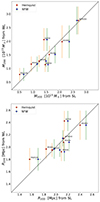 |
Fig. 6. Upper panel: comparison between the SL-based M200c measurements and those based on the WL. Lower panel: Comparison between the SL-based R200c measurements and those based on the WL. These measurements are very close to a 1:1 ratio, especially those relative to the most regular galaxy clusters. |
We note that the R200c and M200c values we obtained from the results of our fits, especially those that were derived with the Hernquist profile, are very close to the weak-lensing measurements in the literature (Jee et al. 2014; Medezinski et al. 2016; Umetsu et al. 2018). Conversely, the M200c and R200c values obtained from the NFW profiles are slightly overestimated with respect to the Hernquist profiles. The less regular clusters, that is, A2744, M0416, and ACT0102, also agree very well between the SL and WL measurements, even though their scale radii are different (see Section 5). The reason is that the larger-scale radii are compensated for by lower central densities, following the behavior that we showed in Figure 7 and discussed in Section 6.2. This balance between the parameters means that the R200c and M200c values of the less regular galaxy clusters are as valid as those of the more regular clusters. The excellent match between the SL and WL measured M200c values shows overall that high-quality SL models, with low RMS and tens of multiple images, extend the information-extraction capabilities to regions that lie well beyond the borders of the multiple-image positions.
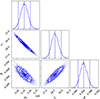 |
Fig. 7. Corner plot of the beta model parameters for the galaxy cluster M1206. The vertical dashed lines in the histograms represent from left to right the 16th, 50th, and 84th percentiles of the distribution, and in the 2D histograms the 0.5, 1, 1.5, and 2 σ equivalent contours are drawn. The central density ρ0 and the scaling radius rs are strongly correlated. This behavior is observed for all models of each galaxy cluster. |
6. Discussion
The datasets at our disposal, as explained in Section 2.2, consist of cumulative projected total mass profiles. The lack of information about the third spacial dimension is inconvenient for two reasons. First, the real geometry of the structure is hidden by the projection on the sky plane, hence the assumptions for the models we made cannot be completely verified, and second, the stacking of information due to the projection operation may soften some features in the projected mass profile, such as mass substructures.
6.1. Assumption of spherical symmetry
In this section, we discuss the effects of our assumption of spherical symmetry for the clusters on the results. The hypothesis of spherical symmetry has the great advantage of resulting in simple and analytical solutions to all the deprojected massmodels listed in Section 3.1. However, it excludes a possible (and often observed, e.g., Despali et al. 2014; Bonamigo et al. 2015) bi- or triaxial configuration. Moreover, the spherical assumption does not take the specific characteristics of galaxy clusters into account, such as mass substructures, which may introduce a perturbation in the total mass distribution that is neglected in our hypothesis. Overall, we consider the spherical symmetry approximation a good tradeoff between its limitations and advantages because its simplicity allows us not only to have analytical solutions, but also to handle a limited number of free parameters that can immediately be compared with the measurements or with other models (as we did for the  and rS − R200crelations).
The impact of the spherical symmetry assumption is hard to quantify and is different from one cluster to the next. However, we can quantify the impact of this hypothesis with two different tests. First, we can examine the reduced χ2 values presented in Table 2. As we mentioned in Section 4, these values are often significantly higher than one. This might suggest that spherical models are too simplistic for an accurate representation of the projected total mass profiles. The very small error bars on the measured quantities cause the high values of the χ2. We also note that we modeled some galaxy clusters with the assumption of spherical symmetry that are known to be composed of more complex mass substructures (see Section 3.1). The performances of the spherical models are particularly good in terms of relative errors, however. In Figure 3 we illustrate the absolute values of the relative errors between the projected total mass measured from the SL analysis and our models. For more than 90% of the considered radii, the relative errors δR (at least of the best-fitting model) are clearly below the 5% threshold (drawn as the horizontal red lines). This fact shows that although the reduced χ2 values might suggest that the spherical models are not very accurate, the relative difference in measured and modeled total mass is particularly small. For these reasons, we consider our models as a competitive solution for an interpretation of the projected total mass profiles in the selected sample of galaxy clusters.
6.2. Projection effects
In this section, we discuss the projection effect of the total mass distribution, resulting from the SL analysis, on the characteristics of the final profiles. As shown by Bonamigo et al. (2017, 2018), some clusters we studied present evident mass substructures in their cores. In these works, the massive substructures were taken into account in the strong-lensing analyses. Except for a kink in the innermost regions (see Figure 2 and Sections 4.1, 4.2, 4.3), the cumulative total mass profiles show no evident features or irregularities caused by the substructures. This behavior is related to the nature of the SL analysis, which measures the total mass that is enclosed within a certain area (that is, within a projected radius) and sums all the relevant mass contributions on the projected plane. Consequently, the mass perturbations introduced by the substructures become less relevant and are not detected in the cumulative projected total mass profiles. Based on this argument, we neglected the presence and effects of any substructure in our sample of galaxy clusters.
The projected quantities also affect the parameter values of the adopted models. Two of the free parameters of the chosen mass models are indeed strongly correlated (models with three free parameters show no preferential pairs of correlated parameters). As an example, we show in Figure 7 the parameter degeneracies that we obtained when we fit the total mass profile of M1206 with the beta model. The values of the central density ρ0 and the scaling radius rs are strongly correlated. A similar behavior is found in every plot of the posterior distributions. The degeneracy between ρ0 and rs for these models is indeed harder to break when some information is lacking due to the projection.
Results of the moving center tests.
6.3. Robustness tests
As mentioned in Section 2.2, we tested whether the values of best-fit parameters of the mass models changed significantly when the center of the circular regions was moved to a different point and the total mass distribution within the new regions was fit accordingly. We also tested whether the values of the best-fit parameters changed appreciably when the maximum radii of the circular areas were increased while the centers were kept fixed.
We chose to change the centers of A2744, M0416, and ACT0102 because they are the least regular clusters in our sample. Specifically, for A2744, we measured a new total mass profile centered on the southern BCG of the galaxy cluster (called BCG-S in Bergamini et al. 2023) in contrast to the original mass profile that was centered on BCG-N. For M0416, we measured two new total mass profiles, one centered on the southern BCG, and the other located in the mean point between the two BCGs. For ACT0102, we measured two new profiles centered on the middle of the northern clump3 and on the mean point between this latter position and the BCG. We used the Hernquist model when the profiles were centered on a BCG and the NIS model for the other positions. The choice of testing only the Hernquist model was justified by the long computational times required to explore all the models, and because this model was adopted to calibrate the scaling laws in Section 5. On the other hand, we decided to test the NIS model in the BCG midpoints of M0416 and ACT0102 because the most relevant mass component is the large-scale DM halo of the galaxy clusters at these locations. It is characterized by a nearly flat profile in its core. We report in Table 5 the results for the original projected mass fits and the outcomes of the tests on the new regions for A2744, M0416, and ACT0102. We adopt different models for different center positions and therefore include in Table 5 the total mass value within 500 kpc computed with the best-fit parameter values. The distance of 500 kpc is the best compromise between the innermost regions of the clusters (where the multiple images are detected) and the outer regions, where the total mass values that we can obtain from our fitted models are fully based on an extrapolation. The different models are in good agreement between each other, which indicates that the choice of the center position is not the most relevant factor when the shape of the cumulative total mass profiles is to be determined. Moreover, Figure 8 shows that the relative differences ΔSL of the new fits with the shifted centers are still clearly below the 5% treshold for the vast majority of the considered radii. We conclude that when the centers of the projected total mass profiles are moved, our spherical models reproduce cumulative total mass values that are consistent with previous results even when the parameter values change slightly.
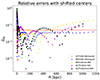 |
Fig. 8. Relative differences ΔSL (absolute values) of the mass models fit on the projected profiles with shifted centers. As in Figure 3, the horizontal red line in the plot shows the 5% threshold. |
We chose the increasing radius test for M0329 and A2744 because the first cluster is representative of the regular galaxy cluster class (in which we count RXJ2129, AS1063, M1931, M1206, M0329, and M2129) and the second represents the less regular class (in which we list A2744, M0416 and ACT0102). We performed this test in two ways: For A2744, we tested all our four best models (NFW, NIS, Hernquist, and beta) assuming a maximum radius of 190″ from the BCG-N, so that the resulting area also enclosed the more external clumps G1, G2, and G3 (see Bergamini et al. 2023 for reference). For M0329 we instead changed the maximum radius the radius five times and kept the Hernquist model fixed.
Table 6 shows that the growth of the maximum radius for M0329 does not affect the parameter values much even when the considered area is 36 times larger than the original. This behavior is reflected in the total mass values within 500 kpc, which do not change significantly when the maximum radius is increased. A2744 presents a more complex situation, in which the parameter values vary with respect to the original choice of the mass profile center because an unregular cluster like A2744 can show local peaks in the mass distribution at large radii (in the case of A2744, these peaks correspond to clumps G1, G2, and G3). This can significantly influence the behavior of the total mass fits. Consequently, the total mass values within 500 kpc can become inconsistent although the relative difference between them lies below 15%. We note, however, that the variation in the parameters follows the correlation pattern described in Section 6.2: an increase in the central density that is counterbalanced by a decrease in the scaling radius. This behavior can be also observed for M0329, but it is not as pronounced there.
Results of the increasing radius tests.
Although we did not repeat these tests for every cluster in our sample, there are further arguments in favor of the robustness of our measurements. First, for the galaxy clusters of the regular class, it would not be very useful to measure the projected mass profile with a center that is shifted from the original center because this type of galaxy clusters has a single well-determined peak in the total mass density (e.g., Figure 2 in Bonamigo et al. 2018 for AS1063 and M1206). For all the unregular clusters, we instead tested the effects of the center shift because the multiple peaks in the total mass density prevented us from unequivocably determining the position for the cluster center. Second, the radii of the set of circles in which the total mass is measured were spaced logarithmically so that the innermost regions of the clusters could be sampled better, where the strong-lensing measurements are more robust. Even though we did not perform the increasing radius test on every galaxy cluster, we therefore expect that the model parameter values we measured by fitting on smaller regions do not change significantly when the size of the region is increased. This conclusion holds true especially for the most regular galaxy clusters in our sample. The previous argument is supported by an additional third test. Specifically, we verified that when the models (computed with the parameters fit in the regions that are showed in Figure 1) were extended to larger radii, the reduced χ2 values did not varysignificantly.
7. Conclusions
We studied the galaxy clusters RXJ2129, A2744, AS1063, M1931, M0416, M1206, M0329, M2129, and ACT0102 (see Table 1 and Figure 1). These nine well-studied massive galaxy clusters lie at intermediate redshifts (0.2 < z < 0.9). Their rich photometric and spectroscopic datasets mainly come from the CLASH, HFF, and CLASH-VLT programs combined with MUSE measurements and allowed detailed studies of their mass composition (Caminha et al. 2016, 2017a,b; Bonamigo et al. 2017, 2018; Bergamini et al. 2019; Caminha et al. 2019, 2023; Bergamini et al. 2023) and measurements of their cumulative radial total mass profiles. We performed the analysis we summarize below.
-
We selected simple one-component spherically symmetric models (see Section 3.1), with two or three free parameters that were simply related to the characteristic quantities of galaxy clusters in order to fit their projected total mass profiles. The numeric fits were performed with a Monte Carlo Bayesian analysis of the posterior probability distribution of the free model parameters (Section 3.2).
-
The results of the MCMC fits (Figure 2) showed that NFW, Hernquist, and beta model profiles are generally well suited to reproducing the projected mass profiles of the selected galaxy clusters. Although the best mass model varies from one cluster to the next, the NIS model is unsuitable in all cases.
-
We employed the results from the projected total mass profiles to derive new possible scaling relations. In particular, we compared the total mass values of the Hernquist model (
 ) for each galaxy cluster with the M200c values measured from WL analyses. We also compared the scale lengths rS of the Hernquist model and the R200c value for each galaxy cluster and searched for a possible relation.
 -
The comparison between SL-based (
 , rS) and WL-based measurements (M200c, R200c) led to different scaling relations. We found a linear scaling law for
  -M200c and rS-R200c, and we tested a power-law dependence for the
 -M200c relation (Figures 4 and 5). We performed this test on a reduced galaxy cluster sample, from which we discarded the least regular clusters.
 -
Although they were applied to very different regions of galaxy clusters, the correspondence between SL and WL measured M200c (and R200c) values in Figure 6 showed that these two techniques can be linked under the proper conditions. This relation can be further investigated and exploited in future studies.
We draw three main conclusions from our modeling of galaxy clusters. First, different mass models can reproduce the projected total radial mass profiles equally well. For our galaxy cluster sample, the best-fitting models were the Navarro–Frenk–White (NFW, Navarro et al. 1997), the Hernquist (Hernquist 1990), and the beta models. Second, although galaxy clusters may present a complex structure, single-component spherical models can reconstruct the inner mass distribution of the whole structure with very small relative errors (≲5%). Last, we found two scaling laws between the SL ( , rS) and WL (M200c, R200c) measured quantities. The
  and rS − R200c relations can be used as powerful tools in future studies on the total mass distribution in galaxy clusters. This link was further enforced by the excellent match between the SL and WL measured M200c values as well as between the R200c values.
Our work provided new insights into the behavior of the total mass distribution in massive galaxy clusters. The study of the total mass profiles in galaxy clusters through well-known analytical models can be further improved in order to have a fair balance between a simple description of these objects and an accurate tool for further measurements. As a first future development, we suggest to enlarge the sample of analyzed galaxy clusters: This would allow us to improve the scaling laws that we found in this work in an extended effort to reduce the scatter of these relations. Through the modeling performed in this work, we set the basis for a sample of galaxy clusters with simple but accurate total mass models that can immediately render their most important properties. Moreover, a determination of the quantities that can be measured through both SL and WL techniques might lead to surprising new methods for the study of galaxy clusters.
In the paper by Umetsu et al. (2018), the authors employ a cosmological model slightly different from ours, setting Ωm = 0.27, ΩΛ = 0.73, and H0 = 70 km s−1 Mpc−1. However, we have checked that the effective change in the critical surface mass density Σcrit in the WL analysis introduced by these different parameter values is ≲2%. Therefore, we neglect the errors related to this change, since they are significantly smaller than the statistical uncertainties reported by the authors.
References
- Bacon, R., Accardo, M., Adjali, L., et al. 2010, in Ground-based and Airborne Instrumentation for Astronomy III, eds. I. S. McLean, S. K. Ramsay, & H. Takami, SPIE Conf. Ser., 7735, 773508 [Google Scholar]
- Bahcall, N. A., & Kulier, A. 2014, MNRAS, 439, 2505 [Google Scholar]
- Balestra, I., Mercurio, A., Sartoris, B., et al. 2016, ApJS, 224, 33 [Google Scholar]
- Bergamini, P., Rosati, P., Mercurio, A., et al. 2019, A&A, 631, A130 [NASA ADS] [CrossRef] [EDP Sciences] [Google Scholar]
- Bergamini, P., Acebron, A., Grillo, C., et al. 2023, ApJ, 952, 84 [NASA ADS] [CrossRef] [Google Scholar]
- Bezanson, R., Labbe, I., Whitaker, K. E., et al. 2024, ApJ, 974, 92 [NASA ADS] [CrossRef] [Google Scholar]
- Biviano, A., Rosati, P., Balestra, I., et al. 2013, A&A, 558, A1 [Google Scholar]
- Biviano, A., Moretti, A., Paccagnella, A., et al. 2017, A&A, 607, A81 [NASA ADS] [CrossRef] [EDP Sciences] [Google Scholar]
- Bonamigo, M., Despali, G., Limousin, M., et al. 2015, MNRAS, 449, 3171 [NASA ADS] [CrossRef] [Google Scholar]
- Bonamigo, M., Grillo, C., Ettori, S., et al. 2017, ApJ, 842, 132 [NASA ADS] [CrossRef] [Google Scholar]
- Bonamigo, M., Grillo, C., Ettori, S., et al. 2018, ApJ, 864, 98 [Google Scholar]
- Braglia, F. G., Pierini, D., Biviano, A., & Böhringer, H. 2009, A&A, 500, 947 [NASA ADS] [CrossRef] [EDP Sciences] [Google Scholar]
- Caminha, G. B., Grillo, C., Rosati, P., et al. 2016, A&A, 587, A80 [NASA ADS] [CrossRef] [EDP Sciences] [Google Scholar]
- Caminha, G. B., Grillo, C., Rosati, P., et al. 2017a, A&A, 600, A90 [NASA ADS] [CrossRef] [EDP Sciences] [Google Scholar]
- Caminha, G. B., Grillo, C., Rosati, P., et al. 2017b, A&A, 607, A93 [NASA ADS] [CrossRef] [EDP Sciences] [Google Scholar]
- Caminha, G. B., Rosati, P., Grillo, C., et al. 2019, A&A, 632, A36 [NASA ADS] [CrossRef] [EDP Sciences] [Google Scholar]
- Caminha, G. B., Grillo, C., Rosati, P., et al. 2023, ApJ, 678, A3 [Google Scholar]
- Coe, D., Salmon, B., Bradač, M., et al. 2019, ApJ, 884, 85 [Google Scholar]
- Despali, G., Giocoli, C., & Tormen, G. 2014, MNRAS, 443, 3208 [Google Scholar]
- Elíasdóttir, Á., Limousin, M., Richard, J., et al. 2007, ArXiv e-prints [arXiv:0710.5636] [Google Scholar]
- Ettori, S. 2000, MNRAS, 311, 313 [NASA ADS] [CrossRef] [Google Scholar]
- Foreman-Mackey, D., Hogg, D. W., Lang, D., & Goodman, J. 2013, PASP, 125, 306 [Google Scholar]
- Gauss, K. F. 1813, Carl Friedrich Gauss Werke, 3, 123 [Google Scholar]
- Hernquist, L. 1990, ApJ, 356, 359 [Google Scholar]
- Huss, A., Jain, B., & Steinmetz, M. 1999, MNRAS, 308, 1011 [Google Scholar]
- Jee, M. J., Hughes, J. P., Menanteau, F., et al. 2014, ApJ, 785, 20 [NASA ADS] [CrossRef] [Google Scholar]
- Jullo, E., Kneib, J. P., Limousin, M., et al. 2007, New J. Phys., 9, 447 [Google Scholar]
- Jullo, E., Natarajan, P., Kneib, J. P., et al. 2010, Science, 329, 924 [Google Scholar]
- Kassiola, A., & Kovner, I. 1993, ApJ, 417, 450 [Google Scholar]
- Kneib, J. P., Ellis, R. S., Smail, I., Couch, W. J., & Sharples, R. M. 1996, ApJ, 471, 643 [Google Scholar]
- Kravtsov, A. V., & Borgani, S. 2012, ARA&A, 50, 353 [Google Scholar]
- Le Fèvre, O., Saisse, M., Mancini, D., et al. 2003, in Instrument Design and Performance for Optical/Infrared Ground-based Telescopes, eds. M. Iye, & A. F. M. Moorwood, SPIE Conf. Ser., 4841, 1670 [CrossRef] [Google Scholar]
- Lotz, J. M., Koekemoer, A., Coe, D., et al. 2017, ApJ, 837, 97 [Google Scholar]
- Mann, A. W., & Ebeling, H. 2012, MNRAS, 420, 2120 [NASA ADS] [CrossRef] [Google Scholar]
- Medezinski, E., Umetsu, K., Okabe, N., et al. 2016, ApJ, 817, 24 [NASA ADS] [CrossRef] [Google Scholar]
- Natarajan, P., & Kneib, J.-P. 1997, MNRAS, 287, 833 [Google Scholar]
- Navarro, J. F., Frenk, C. S., & White, S. D. M. 1997, ApJ, 490, 493 [Google Scholar]
- Owers, M. S., Randall, S. W., Nulsen, P. E. J., et al. 2011, ApJ, 728, 27 [Google Scholar]
- Postman, M., Coe, D., Benítez, N., et al. 2012, ApJ, 199, 25 [Google Scholar]
- Rosati, P., Balestra, I., Grillo, C., et al. 2014, The Messenger, 158, 48 [NASA ADS] [Google Scholar]
- Sartoris, B., Biviano, A., Rosati, P., et al. 2020, A&A, 637, A34 [NASA ADS] [CrossRef] [EDP Sciences] [Google Scholar]
- Steinhardt, C. L., Jauzac, M., Acebron, A., et al. 2020, ApJS, 247, 64 [Google Scholar]
- Treu, T., Schmidt, K. B., Brammer, G. B., et al. 2015, ApJ, 812, 114 [Google Scholar]
- Treu, T., Roberts-Borsani, G., Bradac, M., et al. 2022, ApJ, 935, 110 [NASA ADS] [CrossRef] [Google Scholar]
- Umetsu, K., Sereno, M., Tam, S.-I., et al. 2018, ApJ, 860, 104 [Google Scholar]
Appendix A: Parameter scaling with M200c
We plot in Figure A.1 the relation between the best-fitting parameters of the NFW and Hernquist profile for each galaxy cluster in the sample. We notice that the larger the scale radii rs are, the higher are the corresponding M200c values. This fact can be interpreted as a consequence of the concentration-mass relation (e.g. Biviano et al. 2017). Regarding the ρ0 values, we can justify their behavior by considering the anticorrelation between parameters that we discuss in Section 6.2. It is then straightforward to see that the most massive galaxy clusters are also those with the lowest scale density.
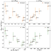 |
Fig. A.1. Relation between the best-fitting parameters of the NFW and Hernquist profile for each galaxy cluster in the sample. On the left column we plot the ρ0 vs M200c relation, while on the right we plot rs vs M200c. |
All Tables
List of the galaxy clusters with relevant information for the strong-lensing analyses.
Values of the reduced χ2 for each mass profile fit to the sample of galaxy clusters
Median values and 1σ confidence level errors of the parameters for each total mass model for each galaxy cluster.
All Figures
|
Fig. 1. The galaxy clusters of our sample. The background images are from the HST and JWST optical/infrared passbands. The blue circles represent the positions of the multiple images employed in the strong-lensing studies by Caminha et al. (2019, 2023) and Bergamini et al. (2019, 2023). The red circles show the area surrounding the multiple images that we considered for the measurement of the projected total mass profiles. The red crosses indicate the centers of the red circles and the origin point of each projected total mass profile. The green lines represent the radii of the red circles, whose length is shown near them. |
| In the text | |
|
Fig. 2. Cumulative projected total mass profiles for the nine clusters in the sample. The red dots show the measured values with their corresponding errors (1σ error bars), and the solid lines represent the best fits of the MSL(R) profiles of each mass model (NFW, NIS, Hernquist, and beta model). The shaded regions represent the 1σ (68%) confidence regions. Each dashed rectangle is zoomed-in the upper left corner of each plot. |
| In the text | |
|
Fig. 3. Absolute values of the relative differences between the measured and modeled cumulative projected total mass profiles rescaled to the measured profiles (ΔSL; see Equation (10)) for each galaxy cluster. The horizontal red line in each plot represents the 5% threshold. |
| In the text | |
|
Fig. 4. Scaling relation between the total mass from the Hernquist profile, |
| In the text | |
|
Fig. 5. Relation between the fitted scale radii of the Hernquist profile, rs, and the R200c values obtained from the available values of M200c. The solid line shows the linear best fit, and its corresponding 1σ uncertainty is represented by the shaded zone. |
| In the text | |
|
Fig. 6. Upper panel: comparison between the SL-based M200c measurements and those based on the WL. Lower panel: Comparison between the SL-based R200c measurements and those based on the WL. These measurements are very close to a 1:1 ratio, especially those relative to the most regular galaxy clusters. |
| In the text | |
|
Fig. 7. Corner plot of the beta model parameters for the galaxy cluster M1206. The vertical dashed lines in the histograms represent from left to right the 16th, 50th, and 84th percentiles of the distribution, and in the 2D histograms the 0.5, 1, 1.5, and 2 σ equivalent contours are drawn. The central density ρ0 and the scaling radius rs are strongly correlated. This behavior is observed for all models of each galaxy cluster. |
| In the text | |
|
Fig. 8. Relative differences ΔSL (absolute values) of the mass models fit on the projected profiles with shifted centers. As in Figure 3, the horizontal red line in the plot shows the 5% threshold. |
| In the text | |
|
Fig. A.1. Relation between the best-fitting parameters of the NFW and Hernquist profile for each galaxy cluster in the sample. On the left column we plot the ρ0 vs M200c relation, while on the right we plot rs vs M200c. |
| In the text | |
Current usage metrics show cumulative count of Article Views (full-text article views including HTML views, PDF and ePub downloads, according to the available data) and Abstracts Views on Vision4Press platform.
Data correspond to usage on the plateform after 2015. The current usage metrics is available 48-96 hours after online publication and is updated daily on week days.
Initial download of the metrics may take a while.