| Issue |
A&A
Volume 675, July 2023
|
|
|---|---|---|
| Article Number | A56 | |
| Number of page(s) | 12 | |
| Section | Cosmology (including clusters of galaxies) | |
| DOI | https://doi.org/10.1051/0004-6361/202346545 | |
| Published online | 30 June 2023 | |
An IllustrisTNG view of the caustic technique for galaxy cluster mass estimation
1
Department of Astronomy and Physics, Saint Mary’s University, 923 Robie Street, Halifax B3H3C3, Canada
e-mail: This email address is being protected from spambots. You need JavaScript enabled to view it.
2
Smithsonian Astrophysical Observatory, 60 Garden Street, Cambridge, MA, 02138
USA
3
Dipartimento di Fisica, Università di Torino, Via P. Giuria 1, 10125 Torino, Italy
4
Istituto Nazionale di Fisica Nucleare (INFN), Sezione di Torino, Via P. Giuria 1, 10125 Torino, Italy
Received:
30
March
2023
Accepted:
31
May
2023
Abstract
The TNG300-1 run of the IllustrisTNG simulations includes 1697 clusters of galaxies with M200c > 1014 M⊙ covering the redshift range 0.01 − 1.04. We built mock spectroscopic redshift catalogs of simulated galaxies within these clusters and applied the caustic technique to estimate the cumulative cluster mass profiles. We computed the total true cumulative mass profile from the 3D simulation data, calculated the ratio of caustic mass to total 3D mass as a function of cluster-centric distance, and identified the radial range where this mass ratio is roughly constant. The ratio of 3D to caustic mass on this plateau defines ℱβ. The filling factor, ℱβ = 0.41 ± 0.08, is constant on a plateau that covers a wide cluster-centric distance range, (0.6 − 4.2) R200c. This calibration is insensitive to redshift. The calibrated caustic mass profiles are unbiased, with an average uncertainty of 23%. At R200c, the average MC/M3D = 1.03 ± 0.22; at 2 R200c, the average MC/M3D = 1.02 ± 0.23. Simulated galaxies are unbiased tracers of the mass distribution. IllustrisTNG is a broad statistical platform for application of the caustic technique to large samples of clusters with spectroscopic redshifts for ≳200 members in each system. These observations will allow extensive comparisons with weak-lensing masses and will complement other techniques for measuring the growth rate of structure in the Universe.
Key words: galaxies: clusters: general / Galaxy: kinematics and dynamics / methods: numerical
© The Authors 2023
 Open Access article, published by EDP Sciences, under the terms of the Creative Commons Attribution License (https://creativecommons.org/licenses/by/4.0), which permits unrestricted use, distribution, and reproduction in any medium, provided the original work is properly cited.
This article is published in open access under the Subscribe to Open model. This email address is being protected from spambots. You need JavaScript enabled to view it. to support open access publication.
1. Introduction
Massive clusters of galaxies serve as testbeds for cosmological models (e.g., Mantz et al. 2008, 2010, 2015; Rapetti et al. 2009, 2013; Vikhlinin et al. 2009) and as laboratories for galaxy evolution (Lin & Mohr 2004; Oliva-Altamirano et al. 2014; Kravtsov et al. 2018; Sohn et al. 2020, 2022; Golden-Marx et al. 2022). Clusters evolve over the age of the Universe as they accrete material from their surroundings (e.g., Press & Schechter 1974; White & Rees 1978; Bower 1991; Lacey & Cole 1993; Sheth & Tormen 2002; Zhang et al. 2008; Corasaniti & Achitouv 2011; De Simone et al. 2011; Achitouv et al. 2014; Musso et al. 2018).
Measurements of the mass profile of clusters beyond the virial radius are critical for understanding the growth of clusters of galaxies (e.g., Diaferio 2004; Reiprich et al. 2013; Diemer & Kravtsov 2014; Lau et al. 2015; Walker et al. 2019; Rost et al. 2021). Radii typically larger than the fiducial radius R200c1, an estimate of the viral radius, probe the infall region of clusters where they still accrete mass. Mass profiles beyond the approximate virial radius enable estimates of the cluster accretion rate as a function of cosmological epoch (van den Bosch 2002; McBride et al. 2009; Fakhouri et al. 2010; Diemer et al. 2017; De Boni et al. 2016; Pizzardo et al. 2021, 2022). They also provide a route to estimating the splashback radius (e.g., Adhikari et al. 2014; Diemer & Kravtsov 2014; More et al. 2015; Diemer et al. 2017; Contigiani et al. 2019; Xhakaj et al. 2020).
At radii exceeding ∼R200c, the cluster accretes galaxies and dark matter; the system is not in equilibrium (Ludlow 2009; Bakels et al. 2021). Techniques that assume dynamical equilibrium, including virial masses (Zwicky 1937), X-ray masses (Sarazin 1988), and Jeans’ analyses (The & White 1986; Merritt 1987; Binney & Tremaine 2011), are not applicable at large radius. Weak gravitational lensing (Bartelmann 2010; Hoekstra et al. 2013; Umetsu 2020) and the caustic technique (Diaferio & Geller 1997; Diaferio 1999; Serra et al. 2011) do not depend on dynamical equilibrium. Thus these techniques are a route to deriving cluster mass profiles at large radius.
Umetsu et al. (2014, 2016) obtained weak-lensing mass profiles for radii ≲(3 − 5.7) Mpc (a few times R200c). Steadily improving large datasets and sophisticated treatment of systematic issues (Hoekstra 2003; Hoekstra et al. 2011) continually advance the sensitivity and reliability of lensing-mass estimates that extend to a larger radius (Umetsu et al. 2011; Umetsu 2013, 2020).
The caustic technique (Diaferio & Geller 1997; Diaferio 1999) is another strategy for mass estimation beyond R200c. This dynamical method exploits the trumpet-like pattern in the projected phase-space distribution of cluster galaxies that results from the continual infall of matter. The caustic pattern reflects the escape velocity from the cluster. Identification of the region where the phase space density changes sharply enables reconstruction of the mass profile.
Collisionless N-body simulations suggest that the caustic mass profile is an unbiased estimator with a reliability of ∼50% for radii ≲4 R200c. Application of the caustic technique requires dense spectroscopic sampling of a cluster including more than ∼150 galaxies within a radius of ∼3 R200c (Diaferio 1999; Serra et al. 2011).
Rines & Diaferio (2006) and Rines et al. (2013) used two large spectroscopic surveys as a basis for application of the caustic technique to well-defined sets of massive clusters. The Cluster Infall Regions in the Sloan Digital Sky Survey (CIRS) and the Hectospec Cluster Survey (HeCS) surveys characterize the mass profiles of ∼130 clusters of galaxies within a limiting radius of ∼5 Mpc. Pizzardo et al. (2021) used the caustic technique to estimate the mass accretion rate of these clusters based on the mass profile in the range ∼(2 − 3) R200c. Pizzardo et al. (2022) extended the study to stacked clusters from the HectoMAP spectroscopic survey (Sohn et al. 2021a,b). The accretion rates agree with the predictions of N-body simulations of the ΛCDM model, our standard model for cosmological structure formation where the laws of gravity follow general relativity in a flat spacetime with a positive cosmological constant, Λ, and matter content dominated by collisionless cold dark matter (CDM).
Weak lensing and the caustic technique offer complementary approaches for studying the outskirts of clusters of galaxies. Diaferio et al. (2005) and Geller et al. (2013) show that caustic and weak-lensing profiles of the ∼20 HeCS clusters agree within 20 − 30%. Future spectrographs (see, e.g., Dalton et al. 2012; Tamura et al. 2016; Marshall et al. 2019) will enable larger spectroscopic surveys to compare with the ever increasing number of high-quality weak-lensing mass profiles derived from comprehensive, deep photometric surveys.
For application to future ambitious spectroscopic surveys combined with weak lensing, a broad, robust statistical platform for the caustic technique is needed. Previous studies calibrated the caustic mass profiles with N-body simulations where the galaxies were either identified with semi-analytic prescriptions (Diaferio 1999) or associated with random samples of dark matter particles (Serra et al. 2011). Semi-analytical prescriptions for galaxy formation do not capture the full complexity of the hydrodynamics of clusters. Dark matter only simulations rely on the assumption of negligible velocity bias between galaxies and dark matter. In addition, previous work was generally limited to nearby clusters with z ≈ 0. In a first application of the caustic technique to a large hydrodynamical simulation, Armitage et al. (2019) analyzed 30 massive clusters at z = 0 drawn from the Cluster-EAGLE simulation (Barnes et al. 2017; Bahé et al. 2017) and derived a single mass calibration at M200c in 3D space.
To extend statistical calibration of the caustic technique to larger z, we analyze a sample of 1697 clusters from the magneto-hydrodynamical IllustrisTNG simulations (Pillepich et al. 2018; Springel et al. 2018; Nelson et al. 2019), a platform that provides the phase-space distributions of cluster galaxies and dark matter for the same systems. The analysis of simulated galaxy catalogs makes no assumptions about cluster dynamics. IllustrisTNG provides a new, broad statistical platform for application of the caustic technique for systems with z ≲ 1.
In Sect. 2, we review the caustic technique. Section 3 describes the IllustrisTNG simulations, the sample of simulated clusters, and the construction of mock galaxy redshift surveys of the 1697 clusters in the IllustrisTNG sample. Section 4 outlines the calibration of the caustic technique in the redshift range 0.01 − 1.04. Section 5 evaluates the calibrated caustic technique as an estimator of cluster radius and mass. Section 6 compares the simulated galaxies with the dark matter as tracers of the total matter distribution. We also include a survey of some previous applications of the caustic technique. We conclude in Sect. 7.
2. The caustic technique
The caustic technique (Diaferio & Geller 1997; Diaferio 1999; Serra et al. 2011; Serra & Diaferio 2013) estimates the three-dimensional cumulative mass profile (from now on, the “caustic mass profile”) of a cluster from the line-of-sight escape velocity profile of the cluster members, vesc, los(r), where r is the projected cluster-centric distance.
The r − vlos diagram, the line-of-sight velocity with respect to the cluster center, vlos, as a function of r, is the basis for the caustic mass profile. In this space, cluster galaxies delineate a trumpet-shaped pattern with a decreasing amplitude as r increases. The gravitational potential of the cluster causes departure of infalling galaxies from the Hubble flow thus producing this distinctive pattern. Throughout this region, the cluster is not in dynamical equilibrium.
We define the caustics as the symmetric boundaries of the trumpet-shaped region of the r − vlos diagram. The caustic amplitude, 𝒜(r), is half of the distance between the upper and lower caustic. The caustic technique locates the caustics and computes 𝒜(r). Diaferio & Geller (1997) showed that the caustic amplitude approximates the escape velocity profile from a cluster, 𝒜(r)≈vesc, los(r). The square of the caustic amplitude,  , is linked to the gravitational potential of the cluster and thus to its mass profile. The caustics separate member galaxies that lie between the upper and the lower caustic from foreground and background objects.
The caustic technique estimates the mass profile as
 (1)
(1)
where ℱβ is a constant filling factor. In the original formulation of the caustic technique, ℱβ is the average of a function that combines the mass density profile ρ(r), the gravitational potential ϕ(r), and the velocity anisotropy parameter β(r). In hierarchical clustering scenarios, this function depends only weakly on the cluster-centric distance for r ≳ 0.5 R200c (Diaferio 1999; Serra et al. 2011).
Previous studies calibrated ℱβ based on collisionless N-body simulations at z = 0. This approach neglects any bias between dark matter particles and galaxies. Previous studies did not investigate the dependence of ℱβ on redshift. Here we calibrate ℱβ with the IllustrisTNG simulations in the redshift range 0.01 − 1.04.
3. The IllustrisTNG simulations
We extract simulated clusters from the TNG300-1 run of the IllustrisTNG simulations (Pillepich et al. 2018; Springel et al. 2018; Nelson et al. 2019). This sample includes three-dimensional (3D) matter distributions and galaxy mock redshift surveys of the clusters at eleven different redshifts. We describe the simulation in Sect. 3.1, the samples of 3D clusters in Sect. 3.2, and the galaxy mock redshift surveys in Sect. 3.3.
3.1. Basic properties of the IllustrisTNG TNG300-1 simulation
We extract cluster samples from the IllustrisTNG simulations (Pillepich et al. 2018; Springel et al. 2018; Nelson et al. 2019), a set of gravo-magnetohydrodynamical simulations based on the ΛCDM model. Each simulation differs in the size of the simulated volume, the resolution, and the matter content.
The simulations are normalized at z = 127 with the Planck cosmological parameters Planck Collaboration XXVII (2016): cosmological constant ΩΛ0 = 0.6911, cosmological total matter density Ωm0 = 0.3089, baryonic mass density Ωb0 = 0.0486, Hubble constant H0 = 67.74 km s−1 Mpc−1, power spectrum normalisation σ8 = 0.8159, and power spectrum index ns = 0.9667. All of the IllustrisTNG baryonic runs are based on the AREPO code (Springel 2010) which solves the equations of continuum magnetohydrodynamics coupled with Newtonian self-gravity. The simulations include the following baryonic processes: primordial and metal-line cooling in the presence of an ionizing background radiation field, stochastic star formation, stellar evolution with the associated chemical enrichment and mass loss, ISM pressurization resulting from unresolved supernovae, stellar feedback, seeding and growth of supermassive black holes, feedback from supermassive black holes, and the dynamical impact of the amplification of a small primordial magnetic field.
We use the TNG300-1 run of IllustrisTNG. This baryonic run has the highest resolution among the runs with the largest simulated volumes. The comoving box size is 302.6 Mpc on a side. TNG300-1 contains 25003 dark matter particles with mass mDM = 5.88 × 10⁷ M⊙ and the same number of gas cells with average mass mb = 1.10 × 10⁷ M⊙.
Structures in the simulations are identified with a Friends-of-Friends (FoF) algorithm with linking length  , where
  is the mean Lagrangian inter-particle separation. The algorithm is applied only to the dark matter particles. Gas, stars, and black holes are then attached to the same FoF group as their nearest dark matter particle.
The substructures of each FoF group are identified as the gravitationally bound structures within the group by means of the Subfind algorithm (Springel et al. 2001), which runs over all the particle types. A synthetic cluster corresponds to a cluster-mass FoF group. The cluster member galaxies correspond to the substructures identified within the group. We identify the center of each cluster as the center of mass of its most massive, or primary, Subfind group. The center of mass is the sum of the mass-weighted coordinates of all the particles and cells in the substructure.
3.2. 3D information
We build the sample of synthetic clusters starting from the group catalogs compiled by the TNG Collaboration. These catalogs list the global properties of the FoF groups along with the substructures identified by the Subfind algorithm. We use these catalogs to select all of the FoF groups with  .
.
For each FoF halo, we extract a spherical volume from the raw snapshots. This volume is centered on the center of mass of the most massive substructure of the halo. The radius of the volume is  , and it contains all of the matter species including the dark matter, gas, stars, and black holes. From the 3D distribution of matter, we compute the true cumulative mass profile (from now on, the “true mass profile”) of each cluster, M3D(r), in 200 logarithmically spaced bins in the radial range
  . From these profiles, we compute the
  and
and  for each cluster. We use
  to select the final cluster samples of the systems with mass
  . We include clusters in eleven redshift intervals: z = 0.01, 0.11, 0.21, 0.31, 0.42, 0.52, 0.62, 0.73, 0.82, 0.92, and 1.04.
Table 1 lists the number of synthetic clusters, the medians and the 68% widths of the distributions of their masses ( ), and the minimum and the maximum
  at each redshift.
Cluster samples from Illustris TNG300-1.
3.3. Mock redshift surveys
We associate a galaxy mock redshift survey with each simulated cluster. We follow a procedure similar to Pizzardo et al. (2021). They build mock catalogs of clusters from the simulated 3D distribution of the dark matter particles of an N-body simulation. Here we use the distribution of the synthetic galaxies rather than the dark matter particles. This approach produces mock catalogs that automatically include any velocity or spatial bias between dark matter particles and galaxies.
To generate each mock catalog, we extract a squared-basis truncated pyramid centered on the cluster. The smaller basis is closer to the fictitious observer and the pyramid axis is aligned with the x-axis of the simulation that we identify with the line of sight (see Fig. 1 of Pizzardo et al. 2021). The height of the simulated pyramid is 2bL ≈ 177 Mpc. The vertical section of the pyramid at the center is a square with rFOV ≈ 17.7 Mpc on a side.
We use the group catalogs to select all of the substructures with a center of mass within the pyramid. We include substructures within all of the resolved FoF groups regardless of their total mass. To simulate catalogs of cluster galaxies, we consider only the Subfind substructures with stellar mass > 108 M⊙. This selection mimics observable galaxies. Hereafter we refer to these substructures as galaxies.
We use these mock catalogs to estimate the caustic mass profile of the clusters. The basis of this technique is the r − vlos diagram (Sect. 2). To transform the simulations to this observable plane, we need the positions on the sky and the redshifts of the galaxies. Thus, for each simulated cluster, we translate the 3D galaxy coordinates into right ascension α, declination δ, and total redshift z along the line-of-sight.
We translate the original three-dimensional comoving position, rc, i, of each galaxy in the pyramidal volume so that the comoving distance between the observer and the center of the pyramid is  , where E(z) = [(Ωm0 + Ωb0)(1 + z)3 + ΩΛ]1/2 in the flat ΛCDM model, and zs is the redshift of the particular snapshot. The new 3D positions are ri = rs + rc, i. Setting the celestial coordinates of the center of the pyramid to (αc, δc) = (π/2, 0) in radians, standard geometrical transformations yield the celestial coordinates (αi, δi) of the synthetic galaxies. The observed redshift associated with each galaxy is czobs = czi + vlos(1 + zi), where zi is the cosmological redshift obtained by inverting the integral expression of the comoving distance between the observer and the galaxy,
  , and vlos is the component of the peculiar velocity of the galaxy along the observer’s line of sight. Each mock catalog lists the two celestial coordinates and the observed redshift of the constituent galaxies.
The median number of galaxies in the catalogs is 1835, with a 68% range ∼1350 − 2430. The catalogs include foreground and background objects. Within a three-dimensional distance of  , the median number of galaxies in the catalogs lies in the range 172 − 210 (Table 1, Col. 7). Previous studies suggest that this sampling is a solid basis for application of the caustic technique (Serra et al. 2011).
4. Calibration of the caustic technique
The IllustrisTNG simulations provide a platform for the first calibration of caustic mass profiles throughout the redshift range 0.01 − 1.04 with a hydrodynamical simulation. The mock catalogs extracted from the TNG300-1 simulation allow the measurement of ℱβ (Eq. (1)) based on the distribution of simulated galaxies rather than dark matter particles. TNG300-1 also enables the first investigation of possible redshift dependence of ℱβ in the range 0.01 − 1.04. TNG300-1 allows a standardized statistical approach for applying the caustic technique. This statistical approach is independent of the details of individual clusters.
Section 4.1 describes the application of the caustic technique to the mock catalogs. Section 4.2 describes the measurement of filling factor, ℱβ, and its behavior as a function of redshift.
4.1. Caustic mass profiles from the mock catalogs
We apply the caustic technique to 1697 mock catalogs to obtain a set of uncalibrated cumulative caustic mass profiles. Each mass profile is the radial integral of the square of the caustic amplitude (Eq. (1)). The caustic technique uses a hierarchical binary tree based on projected binding energy to select the galaxies used to build the r − vlos diagram. The technique is based on the cluster-centric distances and line-of-sight velocities of the galaxies relative to the angular coordinates and redshift of the cluster center. The center of each synthetic cluster is the position of the most massive substructure within its corresponding FoF halo, analogous to choosing the BCG as the cluster center (Sohn et al. 2022). The position of this substructure is consistent with the center of mass of the FoF halo.
To apply the caustic technique, we smooth the data in the r − vlos diagram to construct a continuous distribution. The parameter hc determines the smoothing scale used to build the continuous density distribution (see, e.g., Eqs. (15)–(17) of Diaferio 1999). We adopt no constraint on the value of the smoothing parameter hc. The standard approach that we follow sets hc with an adaptive kernel that minimizes the integrated square error between the continuous density estimator and the true density determined by the r − vlos diagram (see Eq. (18) of Diaferio 1999). Finally the caustic technique locates the caustics as isocurves of the continuous 2D galaxy number density in phase space.
Figure 1 shows two random examples of typical r − vlos diagrams at z = 0.11 with the associated caustic profiles. The upper (lower) panel shows the result for a cluster with mass larger (smaller) than the median mass. In each panel, points represent simulated galaxies. The blue curves show the caustic profiles. The cluster members delineate a trumpet-shaped pattern in the r − vlos diagram (Sect. 2). The caustic technique locates the caustics which delimit this region. The caustic curves separate cluster members (orange points) from foreground and background objects (green points). The cluster in the upper (lower) panel has 710 (213) caustic member galaxies within  .
.
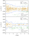 |
Fig. 1. Two examples of simulated r − vlos diagrams at z = 0.11. Blue curves show the caustic profiles. Orange points denote simulated cluster members, green points denote background and foreground galaxies. |
4.2. Measurement of the filling factor
Calibration of the caustic technique with the TNG300-1 simulation has two main steps. First, we identify the radial range where the ratio between the caustic and the true mass profiles is approximately constant. Then, the typical ratio between the two masses on this plateau calibrates the filling factor that normalizes the mass ratio to unity.
In Fig. 2, the two curves show the ratio between the caustic mass profile, MC (= ), and the true mass profile, M3D, as a function of
  for two clusters at redshift z = 0.11. The blue (orange) profile refers to the same cluster used for the top (bottom) r − vlos diagram in Fig. 1.
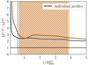 |
Fig. 2. Ratio between the caustic and the 3D true mass profile as a function of the cluster-centric distance |

The ratios show three clear regimes. At small radii,  , there is a rapid decrease. At intermediate cluster-centric distances,
  , there is a plateau. At larger radii, the ratios decrease. In Fig. 2, the colored vertical bands delimit the plateau for the correspondingly colored individual profile.
On the plateau, with a typical extent of  , the ratio between the caustic and the true mass profiles is approximately constant. Figure 2 shows that the caustic mass profiles overestimate the true profiles in this radial range by a nearly constant factor. The mass ratio on the plateaus is a direct measure of the filling factor, ℱβ, for each profile.
The first step in measuring the filling factor is the definition of the plateau. For each redshift sample, we compute the  profiles for each cluster. We then bin the clusters in N = 101 equally spaced bins of
  in the range
  .
.
In building the distribution of the mass ratio profiles, we reject a cluster if its caustic amplitude shrinks to zero at a radius  because the signal-to-noise ratio (S/N) decreases substantially at large cluster-centric distances. On average we remove only 1.5% of the sample for this reason.
For each redshift, we adopt an iterative procedure to identify the radial range of the plateau. We begin by computing σ0, the standard deviation of the mass ratios MC/M3D over the entire radial range  . At each iteration, n, we then compute two new standard deviations. We first omit the bin at the smallest radius from the sample and compute σn, b for the remaining interval. Then we omit only the bin at the largest radius and compute σn, e for all of the remaining bins. The subscripts b and e indicate omission of a bin at the “beginning” and at the “end” of the radial range, respectively. If σn, b < σn, e, we define σn ≡ σn, b and drop the first radial bin. If σn, b > σn, e, σn ≡ σn, e and we drop the last radial bin. Iterating this procedure for n ≤ N − 1 where N = 101 yields a set of shrinking radial intervals with the goal of minimizing the dispersion in the distribution of mass ratios at each step.
As the interval is reduced, the standard deviations first decrease rapidly and then decreases slowly. The onset of the shallower decrease sets the radial limits of the plateau. To locate the plateau numerically, we calculate the set of σn for i = 0, …, N − 11 (where N = 101). We select 11 sequential standard deviations σn, …, σn + 10 for iterations n = 0, 1, 2, etc. Then we calculate ten differences δσn, i = |σn + i − σn + i + 1| where i indicates the ith difference and the bars indicate the modulus of the difference. The average of the ten values of δσn, i is ⟨δσn⟩. For the next set, n + 1, the average is ⟨δσn+1⟩. We define the plateau as the largest interval (or, equivalently, lowest n) where the difference ⟨δσn⟩ is less than ε. We choose ε = 0.001. Our choice is based on the average behavior of ⟨δσn⟩ as a function of n. For the largest candidate plateaus (intervals), or, equivalently, lowest values of n, ⟨δσn⟩ ∼ 0.1. For smaller intervals and larger n, ⟨δσn⟩ steadily decreases. The value reaches ⟨δσn⟩ ≳ 10−4 as the width of the remaining interval becomes  . The choice ε = 0.001 ensures sufficient flatness over the plateau. Figure 2 shows the plateau limits for two of the clusters in the full sample.
In each redshift sample, the sequence of standard deviations may not relax below ε for some clusters. We exclude these clusters in locating the typical plateau. Depending on redshift, we exclude 14.5% to 27.8% of the clusters. On average we exclude 22.6% of the sample.
For each redshift, we compute a single plateau delimited by the median of the smallest radius and the median of the largest radius of the individual cluster plateaus. Finally, we compute a global plateau from the medians of the 11 smallest and the largest radii of the 11 plateaus at fixed redshift. This unique average plateau covers the radial range  .
.
The second step in the calibration procedure exploits the plateau 𝒫 to determine the filling factor as a function of redshift. For each cluster in a redshift bin, we compute the average value of its profile ratio  on the plateau 𝒫. On the interval 𝒫,
  measures the filling factor for that individual kth cluster, ℱβk. The optimal filling factor for the cluster sample in a given bin is the average of the estimates for the individual clusters.
We measure ℱβk for the clusters in each redshift sample. This procedure yields a distribution of ℱβk’s. Figure 3 shows the distribution of individual ℱβk’s for samples at three different redshifts (z = 0.01, 0.52, and 1.04 from left to right, respectively). The distributions have an asymmetric bell shape that is skewed toward large values of ℱβ. The mean of each distribution (dashed line) has a substantial offset with respect to the median (solid line). The means are sensitive to the tails of the distributions, but the medians are located near the peak of the distributions. For each cluster sample, we take the median of the individual ℱβk’s as the optimal filling factor for the redshift interval.
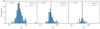 |
Fig. 3. Histograms of the individual ℱβk for 3 cluster samples at different redshifts. Redshift increases from left to right. The thick solid (thin dotted) line in each panel shows the median (mean) of the distribution. |
Table 2 lists the numerical values of the filling factor and its interquartile range in the 11 redshift bins. Figure 4 shows the optimal filling factor as a function of redshift. The error bars show the interquartile ranges. The horizontal line shows the mean filling factor averaged over the 11 redshift ranges,  . Figure 4 and Table 2 show that the optimal filling factor is essentially constant throughout the entire redshift range that we consider. The factor is ℱβ ∼ 0.40 for z < 0.62 and it increases by ∼7% at higher redshifts. The increase with redshift is not statistically significant and is a result of the limited size of the cluster samples at z ≥ 0.62. For z ≥ 0.62 the samples contain fewer than 100 clusters (Table 2, Col. 2). The τ statistic of Kendall’s nonparametric measure of the correlation between ℱβ and redshift is ∼0.06; thus we conclude that ℱβ is independent of redshift. This redshift independence of ℱβ is a distinctive result of the calibration of the caustic technique with Illustris TNG300-1.
 |
Fig. 4. ℱβ as a function of redshift. Error bars show the interquartile range for each redshift sample. The black horizontal line shows the average value of the filling factor over redshift, |

Filling factors.
5. The caustic technique as a cluster mass profile estimator
Based on the optimal filling factors in each redshift bin (Table 2), we evaluate the caustic technique as an estimator of the cluster characteristic radius and mass. For clusters where  lies within the interval 𝒫, we compare the caustic radius
  with
with  . The ratio between the caustic and the true mass profile of the simulated clusters provides the basis for use of the caustic technique as a method for determining cluster mass profiles in observational datasets.
We begin by comparing the radii  ’s estimated from the caustic profiles with the true
  ’s. For each cluster in the simulation (Sect. 4), we compute
  . We remove profiles where
  is indeterminate because it lies at too small a radius to overlap the calibrated range
  where the technique holds. Fewer than 1% of the systems have an indeterminate
  .
.
In Fig. 5 the violet and orange histograms show the distributions of the caustic and true R200c, respectively for all 11 redshift samples. The dash-dotted vertical lines show the interquartile range of the distribution with the corresponding color. The two distributions are similar. The peaks of both distributions are at ∼1 Mpc; the median  is only 1.9% larger than the median
  . Because
  has a larger intrinsic error, the interquartile range of the caustic radii, (0.88 − 1.19) Mpc slightly exceeds the interquartile range of the true 3D radii, (0.90 − 1.14) Mpc.
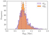 |
Fig. 5. Histograms of |


Figure 6 shows the ratio between the caustic and true R200c’s as a function of  . Each point represents a simulated cluster in one of the 11 redshift samples. In the plot, we omit 12 clusters with a ratio > 1.5 to show the dispersion around a ratio of 1 more clearly. The nine logarithmic bins spanning the range of
  ’s account for the relative sampling densities at the lower and upper extrema of true radii.
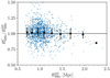 |
Fig. 6. Ratios between |


In each bin, we compute the median and the interquartile range of all the ratios (Fig. 6, black points with error bars). The horizontal line indicates  . The ratios are generally consistent with equality, but the medians of the best sampled bins show that
  overestimates
  slightly. The typical overestimation is ∼1.4% and the dispersion is ∼6.6%. Thus the small overestimate is well within the error in its determination.
We next assess the performance of the caustic technique as a mass estimator in the interval 𝒫. For each cluster in each sample, we normalize the caustic profile by  and obtain
  . Similarly, we normalize the true mass profile by the true
  to determine
  . We then compute the ratio of the two profiles as a function of
  . Finally we compute the median profile of the distribution of individual mass ratio profiles.
The solid black curves in the three panels of Fig. 7 show the median mass ratio profile in the redshift ranges z = 0.01, z = 0.52, and z = 1.04 (left to right). The shaded blue areas show the interquartile range of the profiles. The dashed horizontal line shows equality between the caustic and the true mass profile.
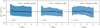 |
Fig. 7. Ratio between the caustic and true mass profiles of the simulated clusters for three different redshifts, z = 0.01, 0.52, and 1.04 (left to right). The solid black curve in each panel shows the median radial profile of the mass ratios. The blue area shows the interquartile range. The black dashed line shows MC(r) = M3D(r). We scale the caustic and true profiles by |


The median caustic and true profiles are on average equal in the interval 𝒫 where we calibrate ℱβ. Averaging over redshift, the median mass ratio in the calibrated range is unbiased and lies between 0.92 and 1.10. On average the caustic technique returns unbiased mass profiles within 10% of the true profiles. The average uncertainty is ∼23%, and is typically ≲29%. At R200c, on average MC/M3D = 1.03 ± 0.22. At 2 R200c, on average MC/M3D = 1.02 ± 0.23.
6. Discussion
The Illustris TNG300 simulations enable the first test of the caustic technique for the estimation of cluster mass profiles based on galaxies extracted from hydrodynamical simulations (Sect. 5). Previous analyses were based either on galaxies identified in N-body simulations with semi-analytical methods (Diaferio 1999) or random samples of dark matter particles (Serra et al. 2011). Armitage et al. (2019) provide the first application of the caustic technique using a hydrodynamical simulation. They derive a single mass calibration at M200c in 3D space at z = 0. In contrast with earlier work, the Illustris TNG300-1 approach covers a broad redshift range 0.01 − 1.04.
Illustris TNG300 provides the basis for testing the caustic technique on both galaxies and dark matter for the same set of clusters. We first address the limitations of the analysis (Sect. 6.1). We then consider evidence for possible bias between simulated galaxies and the dark matter as tracers of the cluster potential (Sect. 6.2). We compare Illustris TNG300-1 results with previous studies in Sect. 6.3.
6.1. Limitations of the analysis
To calibrate the caustic technique with Illustris TNG300-1, we treat galaxies as point-like tracers of the cluster gravitational potential. We apply the caustic technique in the same unconstrained way to every simulated cluster.
Limitations of this approach include possible dependence on the resolution of the simulation and on cluster properties including mass, dynamical state, and shape. Using C-EAGLE simulations with a gas resolution ∼10 times that of TNG300-1 (Barnes et al. 2017; Bahé et al. 2017), Armitage et al. (2019) calibrate the caustic technique at R200c and derive a ℱβ, A = 0.75 (with no quoted error) based on a sample of 30 clusters with a median mass ∼5 × 10¹⁴ M⊙ at z = 0.
To investigate the impact of the Illustris TNG300-1 resolution on the results, we first examine the lower stellar mass cutoff. In the analysis so far, this cutoff is M⋆ > 108 M⊙ (Sect. 3.3). For the TNG300-1 baryonic resolution of ∼1.1 × 10⁷ M⊙ (Nelson et al. 2019), galaxies with the limiting low stellar masses contain only ∼10 baryonic cells. The caustic analysis treats galaxies as point-like tracers of the potential. Thus the analysis should be insensitive to details of the baryonic physics within galaxies.
Comparison with results based on a larger low-M⋆ cutoff, M⋆ > 109 M⊙, probes the dependence on resolution. We explore a low-mass cut of M⋆ > 109 M⊙. This larger low-mass cutoff results in many fewer galaxies per cluster and thus reduces the number of clusters where we can apply the caustic technique in a robust way (Serra et al. 2011). At z = 0, 47 clusters contain more than 150 galaxies above the higher low-mass cutoff within  . Among these 47 clusters, only 34 show the plateau necessary for calculating the filling factor ℱβ in both the original cluster catalog and the catalog with the larger cutoff mass (Sect. 4.2). We compute ℱβ, S and ℱβ, C (Sect. 4) for this subsample of 34 clusters based on the original low-mass cutoff (denoted with subscript S) and the higher low-mass limit (denoted with subscript C). These 34 clusters have median mass M200c ∼ 3.9 × 10¹⁴ M⊙. The larger low-mass cutoff results in a larger filling factor ℱβ, C = 0.57 ± 0.21 but with a substantial error. This filling factor is within 1σ of the estimate for these 34 clusters based on the original mass limit, ℱβ, S = 0.45 ± 0.13. The calibration ℱβ, C = 0.57 ± 0.21 for this subsample is also within 1σ of the global Illustris TNG300-1 result, ℱβ = 0.41 ± 0.08 and overlaps the result of Armitage et al. (2019).
The original catalogs for the 34 clusters contain an average of 389 galaxies within the cluster-centric distance  ; the corresponding catalogs with larger low-mass cutoff typically contain 194 galaxies. To isolate any dependence on relative sampling, we randomly undersample the original catalogs and build new catalogs with the same number of galaxies as in the corresponding catalogs with the higher low-mass cutoff M⋆ = 109 M⊙. Calibrating these caustic profiles leads to a filling factor, ℱβ, U = 0.43 ± 0.11. The effect of undersampling on the calibration is small compared with the impact of the change in the low-mass cutoff.
Calibration based on the original catalogs of the 34 clusters with M200c ∼ 3.9 × 10¹⁴ M⊙ leads to ℱβ, S = 0.45 ± 0.13 slightly exceeding the filling factor ℱβ, 0 = 0.40 ± 0.11 for the entire sample of 224 clusters at z = 0, with median mass M200c ∼ 1.6 × 10¹⁴ M⊙ (Tables 1 and 2). Although this difference in calibration is well within the 1σ error, it hints at a variation of ℱβ with the cluster mass. However, the sample size and the cluster mass distributions in IllustrisTNG are inadequate for statistically significant determination of any potential correlations between ℱβ and mass. The mass distributions peak at ∼1.5 × 10¹⁴ M⊙. Only ∼15% of clusters (∼5 − 35 depending on redshift) have masses ≳(2 − 3)×1014 M⊙.
Theoretical investigations of the caustic technique (Diaferio & Geller 1997; Diaferio 1999; Serra et al. 2011) emphasize that the method is independent of the cluster dynamical state by construction. Scatter in the caustic mass profile reflects both departures from spherical symmetry and the amount of substructure. Biviano & Girardi (2003), Rines et al. (2013), Serra et al. (2011), and Pizzardo et al. (2021) show that results from ensembles of individual clusters like the ones we construct from IllustrisTNG agree with analyses performed by stacking individual clusters within the ensemble. Stacked clusters generally approach spherical symmetry. Qualitative inspection of a random subsample of clusters reveals no obvious correlation between the filling factor and either the dynamical state or the cluster shape. The cluster sample we extract from TNG300-1 is too small to support a robust statistical study that addresses these issues as a function of mass and redshift.
Larger volume hydrodynamical simulations, such MillenniumTNG with its 740 Mpc comoving size, will enable calibration of the caustic technique over the full observed cluster mass range. These larger simulations will naturally include a larger number of the most massive systems than Illustris TNG300-1. These simulations will enable reliable, robust evaluation of the sensitivity of the caustic method to the resolution of the simulation and to cluster properties including mass, dynamical state, shape, and the amount of substructure.
6.2. Comparing the caustic technique for galaxies and dark matter
Galaxies, real or simulated, may be biased tracers of the dark matter distribution. To examine this issue we apply the caustic technique to the dark matter distribution in the same cluster catalogs we explore with simulated galaxies.
For this test we use two catalogs: 255 simulated clusters at z = 0.11 and 178 clusters at z = 0.42 (Table 1). For each cluster, we build one dark matter mock redshift survey following the procedure outlined in Sect. 3.3. We use the Subfind dark matter substructures (rather than galaxies) with stellar mass larger than 107 M⊙. This stellar mass threshold encompasses more than 96% of the total cluster substructures resolved by Subfind. Among these substructures, we select those with total mass larger than 2.1 × 10¹⁰ M⊙; the number of substructures within  is then comparable to the number of galaxies in the corresponding galaxy catalogs. The difference between galaxy and dark matter catalogs is driven by the presence, in the latter, of dark matter subhalos with total mass comparable to galaxies.
The dark matter mock catalogs contain, on average, 62% more substructures than the corresponding number of galaxies. The primary difference is that the dark matter mock catalogs are richer in foreground and background structures than the corresponding galaxy catalogs.
We apply the caustic technique to the dark matter catalogs following Sect. 4.1. For each of the two sets of dark matter catalogs we choose hc as the median of the distribution of the individual hc’s determined from the galaxy mock catalogs at the corresponding redshift (Sect. 4.1). In other words, we locate the caustics from the 2D projected phase-space dark matter densities with the smoothing scale adopted for galaxies. The smoothing parameters are hc = 0.44 and hc = 0.50 for z = 0.11 and z = 0.42, respectively.
We calibrate the filling factor from the dark matter caustic profiles following the procedure in Sect. 4.2. First, we locate the common plateau of the mass profiles from the dark matter catalogs. In this procedure, we end up removing 19.3% of cluster profiles where the plateau is indeterminate. This percentage is analogous to the 22.6% removal of systems based on simulated galaxy catalogs.
The dark matter caustic profiles yield a well defined global plateau with a radial range  . This plateau extends to larger cluster-centric distances than the plateau based on the analogous galaxy catalogs. The more extended dark matter plateau results from the excess of dark matter substructures compared with simulated galaxies. For the galaxy catalogs the extent of the plateau is
  and it is included within the dark matter plateau. We limit the analysis of dark matter caustic profiles to the plateau region defined by the simulated galaxies.
We measure the filling factor from the dark matter caustic profiles following Sect. 4.2. At z = 0.11, ℱβ = 0.37 with an interquartile range 0.30 − 0.46. At z = 0.42, ℱβ = 0.37 with an interquartile range 0.31 − 0.44. These values are in excellent agreement with those obtained from galaxy mock catalogs (Table 2).
We compare the radii  estimated from the galaxy caustic profiles with the corresponding set of
  estimated from the dark matter caustic profiles. There are 272 clusters that allow estimation of both radii on the plateau 𝒫. Figure 8 shows the ratio
  for each cluster (blue points) in the two redshift samples. Black points with error bars show the median and interquartile range of the distribution of these ratios in five logarithmic bins of
  . In the plot, we omit the four clusters with ratios larger than 1.5 and the four clusters with
  larger than 1.75 Mpc. These systems have a negligible effect on the median and the interquartile range in the relevant bins. On average, the radii based on simulated galaxies slightly exceed the radii based on dark matter by ∼3.3%. The typical interquartile range is ∼7%. The small overestimation is thus well within the uncertainty.
 |
Fig. 8.
|


The ratio between the simulated galaxy and dark matter caustic mass profiles of individual clusters provides a platform for assessing the bias between the dark matter and simulated galaxies as tracers of the matter distribution derived from the caustic technique. There are 177 and 110 clusters that support this analysis at z = 0.11 and z = 0.42, respectively.
We normalize the galaxy and the dark matter based caustic mass profiles of each cluster by its  , and obtain
  and
and  , respectively. Then, for each cluster, we compute the ratio profile of the normalized galaxy-based and dark-matter-based mass profiles at fixed
  .
.
Figure 9 shows the median of the individual ratio profiles for z = 0.11 (orange) and z = 0.42 (violet). The shaded areas show the interquartile ranges of the profiles. At z = 0.11, MC is ∼2% smaller than MC, dm; at z = 0.42, MC is ∼4% larger than MC, dm. The difference in the ratio is small compared with the interquartile range of ∼21%. Thus comparison of the caustic technique applied to both galaxy and dark matter catalogs in Illustris TNG300-1 demonstrates that the simulated galaxies are essentially unbiased tracers of the dark matter distribution.
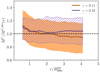 |
Fig. 9. Ratio between caustic profiles based on simulated galaxies and dark matter, for clusters at z = 0.11 (orange) and z = 0.42 (violet). Solid curves show the median radial profile of the mass ratios. The shaded regions areas show the interquartile range. The black dashed line shows MC(r) = MC, dm(r). We scale both profiles by |

6.3. Comparison with previous investigations
We next place the IllustrisTNG results in the context of previous investigations of the caustic technique. In particular, we review various estimates of the filling factor ℱβ = 0.5. We briefly review observational applications of the technique and preview future extensions of the caustic technique to large cluster redshift survey that extend to high redshift. Throughout we emphasize the robustness and redshift independence of ℱβ = 0.41 demonstrated by IllustrisTNG.
The caustic technique was originally developed by Diaferio & Geller (1997) and Diaferio (1999). Other studies of the technique (e.g., Biviano & Girardi 2003; Serra et al. 2011; Gifford & Miller 2013; Gifford et al. 2013; Armitage et al. 2019) adopt a variety of complementary technical approaches including variations in the algorithm for locating the caustics. They may also adopt nonconstant filling factors ℱβ(r). We limit our detailed comparisons to the work of Diaferio & Geller (1997) and Diaferio (1999), where the approach is most similar. Most observational analyses employ the caustic technique based on this work.
Initially Diaferio & Geller (1997) derived ℱβ = 0.5 assuming a hierarchical clustering scenario. Diaferio (1999) used the GIF (Kauffmann et al. 1999) ΛCDM N-body simulation at z = 0 to provide the first simulation-based evaluation of ℱβ(r). This estimate is based on the cluster mass density, the potential, and the velocity anisotropy (see Sect. 2). The value ℱβ = 0.5 is an average value of ℱβ(r) within ∼(1 − 3) R200c.
The IllustrisTNG calibration, ℱβ = 0.41, is typically ∼18% smaller than previous results, but it is based on a broader, more robust platform. The earlier studies are based on collisionless N-body simulations with more limited volume and with lower resolution. In contrast TNG300-1 (Pillepich et al. 2018; Springel et al. 2018; Nelson et al. 2019) is a benchmark for large-scale hydrodynamical simulations. The Illustris TNG300-1 measurement of the filling factor is based only on the relationship between the caustic and the true mass profile of clusters evaluated consistently from the simulated clusters. In contrast with previous work, we extend the measurement of the filling factor beyond z ∼ 0 and reach a limiting z ∼ 1.
Illustris TNG300-1 is a platform for establishing a standardized statistical approach for application of the caustic technique to the outskirts of clusters of galaxies. The identical, unconstrained setup of the analysis applies to every optimally sampled cluster (Sect. 4.1).
Comparisons between caustic and weak-lensing masses (Diaferio et al. 2005; Geller et al. 2013) and caustic and X-ray masses (e.g., Maughan et al. 2016; Andreon et al. 2017; Lovisari et al. 2020; Logan et al. 2022) generally show consistency between the caustic masses obtained with the implementation of Diaferio & Geller (1997) and Diaferio (1999) for ℱβ = 0.5. Both the caustic technique and weak lensing have the strength that they are independent of equilibrium assumptions in contrast with X-ray estimates.
Weak lensing and the caustic technique probe a similar radial range of the cluster mass profile. In contrast, X-ray approaches apply to the smaller range ∼(0 − 1) R200c. In general, the spectroscopic sampling and the variable parameters used to analyze each cluster make it difficult to assess the detailed reasons for differing results.
Geller et al. (2013) show that the caustic mass estimate exceeds the weak-lensing estimate by ∼20 − 30% at radii ∼(0.5 − 1.3) R200c and is ∼20 − 30% below the weak-lensing estimate in the radial range ∼(1.3 − 3) R200c. On average X-ray M200c’s generally exceed the caustic masses by ∼10 − 30% (Maughan et al. 2016; Lovisari et al. 2020; Logan et al. 2022). Andreon et al. (2017) infers caustic masses ∼10% larger than X-ray masses.
The ∼18% smaller (a caustic amplitude correspondingly lower by ∼9%) Illustris TNG300-1 filling factors reduce the caustic mass estimates by approximately this factor. Taken at face value, this revision of the filling factor implies underestimation relative to weak-lensing mass profile at large radii by ∼35 − 40%. Relative to the X-ray M200c, the revised caustic masses are lower by ∼25 − 45%. These simple estimates ignore underlying differences between the Illustris TNG300-1 platform and the application of the caustic technique to previously observed cluster samples.
Optimal sampling of the cluster velocity field is fundamental to robust application of the caustic technique. Redshifts of ≳200 members within a 3D radius of  (e.g., Serra et al. 2011) are optimal. Sparser sampling leads to smaller caustic amplitudes and thus an underestimate of the mass profile.
The CIRS and HeCS survey (Rines & Diaferio 2006; Rines et al. 2013; Sohn et al. 2020) samples provide the best presently available spectroscopic samples. There are typically ≲100 − 150 total spectroscopic members within the probable  .
.
Published observational studies already reflect the dependence of the caustic masses on spectroscopic sampling. For example, out of the 19 clusters in the weak lensing comparison by Geller et al. (2013), the caustic masses of the four best sampled clusters exceed the weak-lensing mass by 20% and up to 50% over the entire radial range. This behavior contrasts with the average underestimate of the caustic masses relative to weak-lensing masses.
Lovisari et al. (2020) computed the ratio between the X-ray mass  and the caustic
  of 25 clusters. On average the ratio
  decreases from 1.30 to 1.03 as the sampling increases. Logan et al. (2022) also show that
  decreases (from ∼1.69 to ∼1.12) as the average number of cluster members increases from 93 to 181. This effect results from the natural underestimate of the caustic amplitude as the sampling becomes poorer.
The Illustris TNG300-1 platform for the caustic technique has no fine tuning of the parameters in the global analysis. Previous application of the caustic technique includes fine tuning of various parameters fundamental to caustic mass estimates. These parameters modify the sample of candidate caustic members, the smoothing parameter, and/or the selection of the isocurve in the continuous projected phase-space of the cluster galaxies. These effects can easily exceed the ∼9% reduction of the caustic amplitude in the Illustris TNG300-1 calibration relative to previous results.
Illustris TNG300-1 provides a solid statistical foundation for the caustic technique, placing the method among the most robust techniques for cluster mass profile reconstruction. Focusing on M200c, X-ray estimates have a ∼5 − 10% scatter in M200c with a possible systematic underestimation of ∼10 − 20% (Ettori et al. 2013). In contrast, at M200c the caustic technique overestimates the true mass by only ∼3% on average. The scatter in the caustic estimates is ∼23%. At the same mass, weak-lensing masses lead to a mild systematic mass underestimate of ≲5% with a scatter of ∼16 − 26% (Becker & Kravtsov 2011; Sommer et al. 2022). This result emphasizes the potential synergy between the caustic and weak-lensing techniques for providing accurate, precise measurement of cluster mass profiles at large radius (Dell’Antonio et al. 2019; Pizzardo et al. 2022).
The Illustris TNG300-1 investigation of the caustic technique provides robust estimates of cluster mass profiles covering a significant radial range extending beyond the virialized region of clusters. The calibration of the caustic technique is stable over a large redshift range, z = 0.01 − 1.04. Upcoming large samples of spectroscopically observed clusters will provide a basis for application of the Illustris TNG300-1 approach to caustic mass estimation. Planned observations with the William Herschel Telescope Enhanced Area Velocity Explorer on WHT (WEAVE, Dalton et al. 2012), the Prime Focus Spectrograph on Subaru (PSF, Tamura et al. 2016), and eventually the Maunakea Spectroscopic Explorer on CFHT (MSE, Marshall et al. 2019) should provide thousands of clusters at redshifts ∼0.5 − 0.6 including spectroscopically determined redshifts of hundreds of members.
7. Conclusion
The IllustrisTNG simulations open a new window on the application of the caustic technique for measuring the masses of clusters of galaxies (Diaferio & Geller 1997; Diaferio 1999). From the TNG300-1 simulation, we construct a catalog of 1697 optimally sampled clusters with M > 1014 M⊙ (Pillepich et al. 2018; Springel et al. 2018; Nelson et al. 2019) that cover the redshift range 0.01 − 1.04. We then derive the total mass including dark matter, stars, gas, and black holes as a function of cluster-centric distance r for each cluster. After applying the caustic technique to each cluster, we calculate the ratio of caustic mass to the total 3D mass, ℱβ, as a function of r and look for the span of r where ℱβ is roughly constant.
The analysis yields a clear plateau where ℱβ = 0.41 ± 0.08 over a large range in cluster-centric distance, (0.6−4.2) R200c. The existence of this plateau enables robust calibration and application of the caustic technique to real systems of galaxies. The technique also provides an unbiased estimate of the true  ,
,  . The range of the plateau, the derived ℱβ, and the estimate for R200c are insensitive to redshift. The caustic technique returns unbiased mass profiles with an average uncertainty of 23%. At R200c, on average MC/M3D = 1.03 ± 0.22; at 2 R200c, on average MC/M3D = 1.02 ± 0.23.
This approach has several distinct advantages over previous investigations. The simulations provide the phase space distributions of cluster galaxies and dark matter for the same systems. The analysis applies a single, unconstrained setup to every cluster to derive the caustic mass profile. We also employ a robust algorithm to find the plateau where ℱβ is roughly constant. The applicable redshift range for this technique, z ≲ 1, is much larger than previous efforts that focus on z ≈ 0.
The caustic amplitude as a function of cluster-centric radius provides an estimate of the local escape velocity. For both galaxies and dark matter in the TNG300-1 simulations, the analysis yields a robust comparison between the mass profiles of both galaxies and dark matter simultaneously. This comparison demonstrates that galaxies are unbiased tracers of the mass distribution.
IllustrisTNG provides a broad statistical platform for application of the caustic technique to large samples of clusters with spectroscopic redshifts for ≳200 members. Instruments including WEAVE on WHT (Dalton et al. 2012), PSF on Subaru (Tamura et al. 2016), and eventually MSE on CFHT (Marshall et al. 2019) will provide the necessary observational foundation. These observations will support extensive comparisons between caustic masses and weak-lensing masses extending to large radius. These two approaches to cluster mass estimation share the strength that they are independent of equilibrium assumptions and they extend outside the virial region. The large future datasets will also support application of the caustic technique as a route for measuring the cluster growth rate as a function of redshift (Diaferio 2004; Adhikari et al. 2014; More et al. 2015; De Boni et al. 2016; Diemer et al. 2017; Walker et al. 2019; Cataneo & Rapetti 2020; Pizzardo et al. 2021, 2022). The cluster mass accretion rate complements other techniques for measuring the growth rate of structure in the Universe.
The next generation of larger volume hydrodynamical simulations such as MillenniumTNG will naturally include a larger number of the most massive systems. They will provide larger samples of highly resolved clusters covering a wide range of mass and redshift. These simulations will enable refinements of the calibration that include reliable, robust evaluation of the sensitivity of the caustic method to the resolution and to cluster properties including mass, dynamical state, shape, and amount of substructure.
In the following, R200c is the radius enclosing an average mass density 200 times the critical density of the Universe at the appropriate redshift. In addition, M200c denotes the corresponding mass.
Acknowledgments
We thank the referee for comments that led to improvements in this paper. We thank Jubee Sohn for insightful discussions. M.P. and I.D. acknowledge the support of the Canada Research Chair Program and the Natural Sciences and Engineering Research Council of Canada (NSERC, funding reference number RGPIN-2018-05425). The Smithsonian Institution supports the research of M.J.G. and S.J.K. A.D. acknowledges partial support from the INFN grant InDark. Part of the present analyses was performed with the computer resources of INFN in Torino and of the University of Torino. This research has made use of NASA’s Astrophysics Data System Bibliographic Services. All of the primary TNG simulations have been run on the Cray XC40 Hazel Hen supercomputer at the High Performance Computing Center Stuttgart (HLRS) in Germany. They have been made possible by the Gauss Centre for Supercomputing (GCS) large-scale project proposals GCS-ILLU and GCS-DWAR. G.C.S. is the alliance of the three national supercomputing centres HLRS (Universitaet Stuttgart), JSC (Forschungszentrum Julich), and LRZ (Bayerische Akademie der Wissenschaften), funded by the German Federal Ministry of Education and Research (BMBF) and the German State Ministries for Research of Baden-Wuerttemberg (MWK), Bayern (StMWFK) and Nordrhein-Westfalen (MIWF). Further simulations were run on the Hydra and Draco supercomputers at the Max Planck Computing and Data Facility (MPCDF, formerly known as RZG) in Garching near Munich, in addition to the Magny system at HITS in Heidelberg. Additional computations were carried out on the Odyssey2 system supported by the FAS Division of Science, Research Computing Group at Harvard University, and the Stampede supercomputer at the Texas Advanced Computing Center through the XSEDE project AST140063.
References
- Achitouv, I., Wagner, C., Weller, J., & Rasera, Y. 2014, JCAP, 2014, 077 [Google Scholar]
- Adhikari, S., Dalal, N., & Chamberlain, R. T. 2014, JCAP, 11, 019 [Google Scholar]
- Andreon, S., Trinchieri, G., Moretti, A., & Wang, J. 2017, A&A, 606, A25 [NASA ADS] [CrossRef] [EDP Sciences] [Google Scholar]
- Armitage, T. J., Kay, S. T., Barnes, D. J., Bahé, Y. M., & Dalla Vecchia, C. 2019, MNRAS, 482, 3308 [NASA ADS] [CrossRef] [Google Scholar]
- Bahé, Y. M., Barnes, D. J., Dalla Vecchia, C., et al. 2017, MNRAS, 470, 4186 [Google Scholar]
- Bakels, L., Ludlow, A. D., & Power, C. 2021, MNRAS, 501, 5948 [NASA ADS] [CrossRef] [Google Scholar]
- Barnes, D. J., Kay, S. T., Bahé, Y. M., et al. 2017, MNRAS, 471, 1088 [Google Scholar]
- Bartelmann, M. 2010, Class. Quant. Grav., 27, 233001 [CrossRef] [Google Scholar]
- Becker, M. R., & Kravtsov, A. V. 2011, ApJ, 740, 25 [NASA ADS] [CrossRef] [Google Scholar]
- Binney, J., & Tremaine, S. 2011, Galactic Dynamics (Princeton: Princeton University Press) [CrossRef] [Google Scholar]
- Biviano, A., & Girardi, M. 2003, ApJ, 585, 205 [NASA ADS] [CrossRef] [Google Scholar]
- Bower, R. G. 1991, MNRAS, 248, 332 [NASA ADS] [CrossRef] [Google Scholar]
- Cataneo, M., & Rapetti, D. 2020, Modified Gravity: Progresses and Outlook of Theories, Numerical Techniques and Observational Tests (World Scientific), 143 [Google Scholar]
- Contigiani, O., Vardanyan, V., & Silvestri, A. 2019, Phys. Rev. D, 99, 064030 [NASA ADS] [CrossRef] [Google Scholar]
- Corasaniti, P. S., & Achitouv, I. 2011, Phys. Rev. Lett., 106, 241302 [NASA ADS] [CrossRef] [Google Scholar]
- Dalton, G., Trager, S. C., Abrams, D. C., et al. 2012, Proc. SPIE, 8446, 220 [Google Scholar]
- De Boni, C., Serra, A. L., Diaferio, A., Giocoli, C., & Baldi, M. 2016, ApJ, 818, 188 [NASA ADS] [CrossRef] [Google Scholar]
- De Simone, A., Maggiore, M., & Riotto, A. 2011, MNRAS, 418, 2403 [CrossRef] [Google Scholar]
- Dell’Antonio, I., Sohn, J., Geller, M. J., McCleary, J., & von der Linden, A. 2019, ApJ, accepted [arXiv:1912.05479] [Google Scholar]
- Diaferio, A. 1999, MNRAS, 309, 610 [CrossRef] [Google Scholar]
- Diaferio, A. 2004, Outskirts of Galaxy Clusters (IAU C195): Intense Life in the Suburbs No. 195 (Cambridge: Cambridge University Press) [Google Scholar]
- Diaferio, A., & Geller, M. J. 1997, ApJ, 481, 633 [NASA ADS] [CrossRef] [Google Scholar]
- Diaferio, A., Geller, M. J., & Rines, K. J. 2005, ApJ, 628, L97 [NASA ADS] [CrossRef] [Google Scholar]
- Diemer, B., & Kravtsov, A. V. 2014, ApJ, 789, 1 [NASA ADS] [CrossRef] [Google Scholar]
- Diemer, B., Mansfield, P., Kravtsov, A. V., & More, S. 2017, ApJ, 843, 140 [NASA ADS] [CrossRef] [Google Scholar]
- Ettori, S., Donnarumma, A., Pointecouteau, E., et al. 2013, Space Sci. Rev., 177, 119 [Google Scholar]
- Fakhouri, O., Ma, C.-P., & Boylan-Kolchin, M. 2010, MNRAS, 406, 2267 [Google Scholar]
- Geller, M. J., Diaferio, A., Rines, K. J., & Serra, A. L. 2013, ApJ, 764, 58 [NASA ADS] [CrossRef] [Google Scholar]
- Gifford, D., & Miller, C. J. 2013, ApJ, 768, L32 [NASA ADS] [CrossRef] [Google Scholar]
- Gifford, D., Miller, C., & Kern, N. 2013, ApJ, 773, 116 [NASA ADS] [CrossRef] [Google Scholar]
- Golden-Marx, J. B., Miller, C. J., Zhang, Y., et al. 2022, ApJ, 928, 28 [NASA ADS] [CrossRef] [Google Scholar]
- Hoekstra, H. 2003, MNRAS, 339, 1155 [NASA ADS] [CrossRef] [Google Scholar]
- Hoekstra, H., Hartlap, J., Hilbert, S., & van Uitert, E. 2011, MNRAS, 412, 2095 [NASA ADS] [CrossRef] [Google Scholar]
- Hoekstra, H., Bartelmann, M., Dahle, H., et al. 2013, Space Sci. Rev., 177, 75 [NASA ADS] [CrossRef] [Google Scholar]
- Kauffmann, G., Colberg, J. M., Diaferio, A., & White, S. D. M. 1999, MNRAS, 303, 188 [NASA ADS] [CrossRef] [Google Scholar]
- Kravtsov, A. V., Vikhlinin, A. A., & Meshcheryakov, A. V. 2018, Astron. Lett., 44, 8 [Google Scholar]
- Lacey, C., & Cole, S. 1993, MNRAS, 262, 627 [NASA ADS] [CrossRef] [Google Scholar]
- Lau, E. T., Nagai, D., Avestruz, C., Nelson, K., & Vikhlinin, A. 2015, ApJ, 806, 68 [NASA ADS] [CrossRef] [Google Scholar]
- Lin, Y.-T., & Mohr, J. J. 2004, ApJ, 617, 879 [Google Scholar]
- Logan, C. H. A., Maughan, B. J., Diaferio, A., et al. 2022, A&A, 665, A124 [NASA ADS] [CrossRef] [EDP Sciences] [Google Scholar]
- Lovisari, L., Ettori, S., Sereno, M., et al. 2020, A&A, 644, A78 [NASA ADS] [CrossRef] [EDP Sciences] [Google Scholar]
- Ludlow, A. D. 2009, PhD Thesis, University of Victoria, Canada [Google Scholar]
- Mantz, A., Allen, S. W., Ebeling, H., & Rapetti, D. 2008, MNRAS, 387, 1179 [CrossRef] [Google Scholar]
- Mantz, A., Allen, S. W., Rapetti, D., & Ebeling, H. 2010, MNRAS, 406, 1759 [NASA ADS] [Google Scholar]
- Mantz, A. B., von der Linden, A., Allen, S. W., et al. 2015, MNRAS, 446, 2205 [Google Scholar]
- Marshall, J., Bolton, A., Bullock, J., et al. 2019, BAAS, 51, 126 [Google Scholar]
- Maughan, B. J., Giles, P. A., Rines, K. J., et al. 2016, MNRAS, 461, 4182 [NASA ADS] [CrossRef] [Google Scholar]
- McBride, J., Fakhouri, O., & Ma, C.-P. 2009, MNRAS, 398, 1858 [NASA ADS] [CrossRef] [Google Scholar]
- Merritt, D. 1987, ApJ, 313, 121 [Google Scholar]
- More, S., Diemer, B., & Kravtsov, A. V. 2015, ApJ, 810, 36 [Google Scholar]
- Musso, M., Cadiou, C., Pichon, C., et al. 2018, MNRAS, 476, 4877 [Google Scholar]
- Nelson, D., Springel, V., Pillepich, A., et al. 2019, Comput. Astrophys. Cosmol., 6, 1 [NASA ADS] [CrossRef] [Google Scholar]
- Oliva-Altamirano, P., Brough, S., Lidman, C., et al. 2014, MNRAS, 440, 762 [NASA ADS] [CrossRef] [Google Scholar]
- Pillepich, A., Springel, V., Nelson, D., et al. 2018, MNRAS, 473, 4077 [Google Scholar]
- Pizzardo, M., Di Gioia, S., Diaferio, A., et al. 2021, A&A, 646, A105 [NASA ADS] [CrossRef] [EDP Sciences] [Google Scholar]
- Pizzardo, M., Sohn, J., Geller, M. J., Diaferio, A., & Rines, K. 2022, ApJ, 927, 26 [NASA ADS] [CrossRef] [Google Scholar]
- Planck Collaboration XXVII. 2016, A&A, 594, A27 [NASA ADS] [CrossRef] [EDP Sciences] [Google Scholar]
- Press, W. H., & Schechter, P. 1974, ApJ, 187, 425 [Google Scholar]
- Rapetti, D., Allen, S. W., Mantz, A., & Ebeling, H. 2009, MNRAS, 400, 699 [NASA ADS] [CrossRef] [Google Scholar]
- Rapetti, D., Blake, C., Allen, S. W., et al. 2013, MNRAS, 432, 973 [NASA ADS] [CrossRef] [Google Scholar]
- Reiprich, T. H., Basu, K., Ettori, S., et al. 2013, Space Sci. Rev., 177, 195 [Google Scholar]
- Rines, K., & Diaferio, A. 2006, AJ, 132, 1275 [Google Scholar]
- Rines, K., Geller, M. J., Diaferio, A., & Kurtz, M. J. 2013, ApJ, 767, 15 [NASA ADS] [CrossRef] [Google Scholar]
- Rost, A., Kuchner, U., Welker, C., et al. 2021, MNRAS, 502, 714 [Google Scholar]
- Sarazin, C. L. 1988, X-ray Emission from Clusters of Galaxies (Cambridge: Cambridge University Press) [Google Scholar]
- Serra, A. L., & Diaferio, A. 2013, ApJ, 768, 116 [NASA ADS] [CrossRef] [Google Scholar]
- Serra, A. L., Diaferio, A., Murante, G., & Borgani, S. 2011, MNRAS, 412, 800 [NASA ADS] [Google Scholar]
- Sheth, R. K., & Tormen, G. 2002, MNRAS, 329, 61 [Google Scholar]
- Sohn, J., Geller, M. J., Diaferio, A., & Rines, K. J. 2020, ApJ, 891, 129 [NASA ADS] [CrossRef] [Google Scholar]
- Sohn, J., Geller, M. J., Hwang, H. S., et al. 2021a, ApJ, 909, 129 [NASA ADS] [CrossRef] [Google Scholar]
- Sohn, J., Geller, M. J., Hwang, H. S., et al. 2021b, ApJ, 923, 143 [NASA ADS] [CrossRef] [Google Scholar]
- Sohn, J., Geller, M. J., Vogelsberger, M., & Damjanov, I. 2022, ApJ, 931, 31 [NASA ADS] [CrossRef] [Google Scholar]
- Sommer, M. W., Schrabback, T., Applegate, D. E., et al. 2022, MNRAS, 509, 1127 [Google Scholar]
- Springel, V. 2010, MNRAS, 401, 791 [Google Scholar]
- Springel, V., White, S. D. M., Tormen, G., & Kauffmann, G. 2001, MNRAS, 328, 726 [Google Scholar]
- Springel, V., Pakmor, R., Pillepich, A., et al. 2018, MNRAS, 475, 676 [Google Scholar]
- Tamura, N., Takato, N., Shimono, A., et al. 2016, Int. Soc. Opt. Photon., 9908, 99081M [Google Scholar]
- The, L. S., & White, S. D. M. 1986, AJ, 92, 1248 [NASA ADS] [CrossRef] [Google Scholar]
- Umetsu, K. 2013, ApJ, 769, 13 [NASA ADS] [CrossRef] [Google Scholar]
- Umetsu, K. 2020, A&ARv, 28, 7 [Google Scholar]
- Umetsu, K., Broadhurst, T., Zitrin, A., Medezinski, E., & Hsu, L.-Y. 2011, ApJ, 729, 127 [NASA ADS] [CrossRef] [Google Scholar]
- Umetsu, K., Medezinski, E., Nonino, M., et al. 2014, ApJ, 795, 163 [NASA ADS] [CrossRef] [Google Scholar]
- Umetsu, K., Zitrin, A., Gruen, D., et al. 2016, ApJ, 821, 116 [Google Scholar]
- van den Bosch, F. C. 2002, MNRAS, 331, 98 [CrossRef] [Google Scholar]
- Vikhlinin, A., Kravtsov, A. V., Burenin, R. A., et al. 2009, ApJ, 692, 1060 [Google Scholar]
- Walker, S., Simionescu, A., Nagai, D., et al. 2019, Space Sci. Rev., 215, 1 [CrossRef] [Google Scholar]
- White, S. D. M., & Rees, M. J. 1978, MNRAS, 183, 341 [Google Scholar]
- Xhakaj, E., Diemer, B., Leauthaud, A., et al. 2020, MNRAS, 499, 3534 [NASA ADS] [CrossRef] [Google Scholar]
- Zhang, J., Ma, C.-P., & Fakhouri, O. 2008, MNRAS, 387, L13 [CrossRef] [Google Scholar]
- Zwicky, F. 1937, ApJ, 86, 217 [NASA ADS] [CrossRef] [Google Scholar]
All Tables
All Figures
|
Fig. 1. Two examples of simulated r − vlos diagrams at z = 0.11. Blue curves show the caustic profiles. Orange points denote simulated cluster members, green points denote background and foreground galaxies. |
| In the text | |
|
Fig. 2. Ratio between the caustic and the 3D true mass profile as a function of the cluster-centric distance |
| In the text | |
|
Fig. 3. Histograms of the individual ℱβk for 3 cluster samples at different redshifts. Redshift increases from left to right. The thick solid (thin dotted) line in each panel shows the median (mean) of the distribution. |
| In the text | |
|
Fig. 4. ℱβ as a function of redshift. Error bars show the interquartile range for each redshift sample. The black horizontal line shows the average value of the filling factor over redshift, |
| In the text | |
|
Fig. 5. Histograms of |
| In the text | |
|
Fig. 6. Ratios between |
| In the text | |
|
Fig. 7. Ratio between the caustic and true mass profiles of the simulated clusters for three different redshifts, z = 0.01, 0.52, and 1.04 (left to right). The solid black curve in each panel shows the median radial profile of the mass ratios. The blue area shows the interquartile range. The black dashed line shows MC(r) = M3D(r). We scale the caustic and true profiles by |
| In the text | |
|
Fig. 8.
|
| In the text | |
|
Fig. 9. Ratio between caustic profiles based on simulated galaxies and dark matter, for clusters at z = 0.11 (orange) and z = 0.42 (violet). Solid curves show the median radial profile of the mass ratios. The shaded regions areas show the interquartile range. The black dashed line shows MC(r) = MC, dm(r). We scale both profiles by |
| In the text | |
Current usage metrics show cumulative count of Article Views (full-text article views including HTML views, PDF and ePub downloads, according to the available data) and Abstracts Views on Vision4Press platform.
Data correspond to usage on the plateform after 2015. The current usage metrics is available 48-96 hours after online publication and is updated daily on week days.
Initial download of the metrics may take a while.