| Issue |
A&A
Volume 682, February 2024
|
|
|---|---|---|
| Article Number | A80 | |
| Number of page(s) | 13 | |
| Section | Cosmology (including clusters of galaxies) | |
| DOI | https://doi.org/10.1051/0004-6361/202244448 | |
| Published online | 05 February 2024 | |
The mass distribution in the outskirts of clusters of galaxies as a probe of the theory of gravity
1
Department of Astronomy and Physics, Saint Mary’s University, 923 Robie Street, Halifax B3H3C3, Canada
e-mail: This email address is being protected from spambots. You need JavaScript enabled to view it.
2
Dipartimento di Fisica, Università di Torino, Via P. Giuria 1, 10125 Torino, Italy
3
Istituto Nazionale di Fisica Nucleare (INFN), Sezione di Torino, Via P. Giuria 1, 10125 Torino, Italy
4
Department of Physics and Astronomy, Western Washington University, Bellingham, WA 98225, USA
Received:
7
July
2022
Accepted:
24
November
2023
Abstract
We show that ς, the radial location of the minimum in the differential radial mass profile M′(r) of a galaxy cluster, can probe the theory of gravity. We derived M′(r) of the dark matter halos of galaxy clusters from N-body cosmological simulations that implement two different theories of gravity: standard gravity in the ΛCDM model, and f(R). We extracted 49 169 dark matter halos in 11 redshift bins in the range 0 ≤ z ≤ 1 and in three different mass bins in the range 0.9 < M200c/1014 h−1 M⊙ < 11. We investigated the correlation of ς with the redshift and the mass accretion rate (MAR) of the halos. We show that ς decreases from ∼3R200c to ∼2R200c when z increases from 0 to 1 in the ΛCDM model. At z ∼ 0.1, ς decreases from 2.8R200c to ∼2.5R200c when the MAR increases from ∼104 h−1 M⊙ yr−1 to ∼2 × 10⁵ h−1 M⊙ yr−1. In the f(R) model, ς is ∼15% larger than in ΛCDM. The median test shows that for samples of ≳400 dark matter halos at z ≤ 0.8, ς is able to distinguish between the two theories of gravity with a p-value ≲10−5. Upcoming advanced spectroscopic and photometric programs will allow a robust estimation of the mass profile of enormous samples of clusters up to large clustercentric distances. These samples will allow us to statistically exploit ς as probe of the theory of gravity, which complements other large-scale probes.
Key words: methods: numerical / galaxies: clusters: general / galaxies: kinematics and dynamics
© The Authors 2024
 Open Access article, published by EDP Sciences, under the terms of the Creative Commons Attribution License (https://creativecommons.org/licenses/by/4.0), which permits unrestricted use, distribution, and reproduction in any medium, provided the original work is properly cited.
This article is published in open access under the Subscribe to Open model. This email address is being protected from spambots. You need JavaScript enabled to view it. to support open access publication.
1. Introduction
According to the standard ΛCDM model, the gravitational dynamics of the Universe and its content is described by General Relativity in a flat space-time with a positive cosmological constant, Λ. The matter content of the Universe mainly consists of cold dark matter (CDM), and baryons are a minor component. In this model, cosmological structures form hierarchically through consecutive mergers of smaller halos into larger halos (e.g., Press & Schechter 1974; White & Rees 1978; Lacey & Cole 1993; Bower 1991; Sheth & Tormen 2002; Zhang et al. 2008; De Simone et al. 2011; Corasaniti & Achitouv 2011; Achitouv et al. 2014; Musso et al. 2018).
For a long time, the outskirts of clusters of galaxies have been regarded as a potentially powerful probe of the model of structure formation and evolution (e.g., Diaferio 2004; Reiprich et al. 2013; Diemer & Kravtsov 2014; Lau et al. 2015; Walker et al. 2019; Rost et al. 2021). At radii larger than the virial radius, this region is linked to the cosmic large-scale structure, which is sensitive to the model of gravity and to the nature of dark matter. Furthermore, unlike the central regions of clusters, comparisons of the dynamical properties of these regions with simulations are more robust because the relevant physical processes are dominated by gravity and not by baryonic physics (e.g., Diemand et al. 2004; Hellwing et al. 2016; Armitage et al. 2018; Velliscig et al. 2014; van Daalen et al. 2014; Shirasaki et al. 2018).
The most widely investigated feature of cluster outskirts is the splashback radius, Rspl, which roughly corresponds to the first apocenter of the orbits of recently accreted material (Adhikari et al. 2014). This radius has an important physical meaning: It separates particles that are orbiting in the gravitational potential of the halo from matter falling onto it (Diemer & Kravtsov 2014; Adhikari et al. 2014; More et al. 2015; Diemer 2020, 2021). For this reason, More et al. (2015) proposed it as the physical boundary of clusters. Diemer & Kravtsov (2014) and More et al. (2015) showed that this feature can be detected as a sudden drop in the logarithmic slope of the halo density profile. These works employed N-body simulations, and they showed that Rspl is usually located at ∼2R200c1 and that it decreases with increasing mass accretion rate (MAR) and redshift.
The splashback radius is a genuine prediction of the hierachical model of structure formation. It is therefore expected to be sensitive to the model of gravity and the nature of dark matter and dark energy (Diemer & Kravtsov 2014; Adhikari et al. 2014, 2018; Contigiani et al. 2019; Banerjee et al. 2020; Diemer 2020; Umetsu 2020). Adhikari et al. (2018) proposed the exploitation of Rspl as a probe of cosmic expansion and the model of gravity for the first time. They used analytical models and N-body simulations to study the impact of dark energy and modifications in gravity on the value of Rspl. They showed that this feature is sensitive both to the w parameter of the equation of state of the dark energy fluid and to two screened modified gravity models, f(R) and nDGP. They pointed out that the outskirts of galaxy clusters are the transition region between the screened and unscreened regimes of modified gravity models, and thus they are the ideal region in which to detect signatures of modified gravity.
In the data, several works detected a change in the slope of the mass density profile at a radius compatible with the expected Rspl (e.g., More et al. 2016; Baxter et al. 2017; Umetsu & Diemer 2017; Chang et al. 2018; Zürcher & More 2019; Shin et al. 2019; Murata et al. 2020; Bianconi et al. 2021; Gonzalez et al. 2021). However, although these results are encouraging, observational estimates are affected by both projection effects and by the fact that we observe galaxies rather than dark matter particles. Dark matter particles and dark matter subhalos, with which galaxies might be associated, do not necessarily share the same apocenter (Diemer et al. 2017). Recent investigations based on hydrodynamical simulations showed that Rspl derived from galaxies or gas particles can substantially differ from Rspl derived from dark matter (Baxter et al. 2021; Deason et al. 2021; O’Neil et al. 2021; O’Neil et al. 2022; Dacunha et al. 2022). These discrepancies behave in a complex way that depends on the halo mass and selection criteria. Therefore, further observational and methodological efforts are required.
High-precision measurements require high-quality spectroscopic and wide-field surveys. These will be available in the near future by ongoing or planned experiments; in addition, an improved understanding of the systematics that affect the methods that are used to estimate the mass profile of clusters is necessary. Currently, weak gravitational lensing (Bartelmann 2010; Umetsu 2020) and the caustic technique (Diaferio 1999; Serra et al. 2011) are the only methods that estimate the cluster mass profile at large cluster-centric distances without relying on dynamical equilibrium. Weak-lensing is steadily improving with the acquisition of large combined spectroscopic and photometric datasets and methodological advancements (Umetsu 2013; Dell’Antonio et al. 2020; Umetsu 2020). Synergies with the caustic technique (Diaferio 1999; Serra et al. 2011) promise unbiased and accurate mass profiles that extend to large radii.
On the theoretical side, we need to thoroughly characterize the dynamics of clusters in their outer region. This plan requires investigating other characteristic radii of cluster outskirts in addition to Rspl. Beyond Rspl, clusters present an extended region in which matter is falling onto them. The radius at which the radial velocity profile has its minimum traces the region of clusters in which the dynamics is a genuine infall (De Boni et al. 2016; Vallés-Pérez et al. 2020; Pizzardo et al. 2021, 2023b). Characteristic radii also arise from the halo-matter bias (Fong & Han 2021; García et al. 2021). These radii depend on the cluster mass and redshift. Because these radii are tightly connected with the cluster MAR, they are probably extremely sensitive to the gravity model. Studies aiming at the quantitative determination of the dependence of these radii on the gravity model are vital for the exploitation of cluster outskirts as a cosmological probe.
Here, we focus on a radius that is different from both Rspl and the radius of the minimum of the radial velocity profile. We consider the radial location, ς, of the minimum of the radial differential mass profile of galaxy clusters, M′(r). We investigate whether ς can distinguish between standard gravity and f(R) gravity based on galaxy cluster halos in wide redshift and mass ranges. The radius ς complements Rspl as a probe of the external region of clusters of galaxies: ς reduces the large errors in Rspl that originate from the logarithmic slope of the density profile, and it can thus in principle be located in individual systems. We prove that although ς and Rspl are not equivalent, they share similar trends with redshift, mass, and MAR.
The paper is organized as follows. In Sect. 2 we present the simulations (Sect. 2.1) and the samples of simulated halos (Sect. 2.2). In Sect. 3 we present our theoretical results: in Sect. 3.1 we compare ς with Rspl, and in Sect. 3.2 we study whether ς can distinguish between two different gravity models. We discuss our results in Sect. 4 and conclude in Sect. 5.
2. Simulations and samples of halos
2.1. DUSTGRAIN simulations
We extracted our samples of simulated halos from DUSTGRAIN (Giocoli et al. 2018), which is a suite of N-body cosmological simulations implementing the standard ΛCDM model and various extensions of General Relativity in the form of f(R). The simulations might include a non-negligible fraction of massive neutrinos. Appendix A reports a basic review of the f(R) model considered in these simulations. For our purposes, we used only the ΛCDM and the fR4 runs; the latter is an f(R) run with scalaron fR0 = −1 × 10⁻⁴ and without massive neutrinos (Ων = 0).
The DUSTGRAIN simulations were normalized at the cosmic microwave background (CMB) epoch with cosmological parameters consistent with the Planck 2015 constraints (Ade et al. 2016). The cosmological matter density is ΩM ≡ ΩCDM + Ωb + Ων = 0.31345, where ΩCDM, Ωb, and Ων are the current CDM, baryonic, and neutrino density parameters, respectively. The DUSTGRAIN simulations had Ωb = 0. Furthermore, they had a cosmological constant ΩΛ = 0.68655, a Hubble constant H0 = 100 h km s−1 Mpc−1, with h = 0.6731, an initial perturbation amplitude 𝒜s = 2.199 × 10⁻⁹, and a power spectrum index ns = 0.9658. The normalization of the power spectrum of the perturbations at the CMB epoch implies that the value of the power spectrum normalization at z = 0, σ8, generally differs among the different simulations. In the two runs relevant for this work, ΛCDM and fR4, σ8 = 0.847 and σ8 = 0.967, respectively2. The box size was 750 h−1 Mpc on a side in comoving coordinates. The simulation contained 7683 collisionless dark matter particles with mass mDM = 8.1 × 10¹⁰ h−1 M⊙ each. Because hydrodynamics is absent, the ΛCDM and the fR4 runs are two standard collisionless N-body simulations with ΩM = ΩCDM = 0.31345 and Ωb = Ων = 0.
The CDM halos were identified with a friends-of-friends (FoF) algorithm (Davis et al. 1985) with linking length  , where
  is the mean Lagrangian interparticle separation. The SUBFIND algorithm (Springel et al. 2001) was run on the FoF groups to identify their gravitationally bound substructures. A synthetic cluster corresponds to the most massive detected substructure, whose most tightly bound particle is the cluster center.
2.2. Samples of simulated halos
For the theoretical investigations presented in this work, we considered the three-dimensional synthetic clusters of DUSTGRAIN (Sect. 2.1) in 11 redshift bins in the range 0 ≤ z ≤ 1. Table 1 lists the main properties of the cluster samples at each redshift: the number of clusters, the median mass, and the median MAR with the 68th percentile ranges of these quantities.
Samples of simulated clusters.
The clusters were separated into low-, intermediate-, and high-mass samples. The low-mass samples contained all the simulated halos with mass M200c ∈ (0.9, 1.1)×1014 h−1 M⊙, and the intermediate- and high-mass samples contained all the halos with mass M200c ∈ (4.0, 6.0)×1014 h−1 M⊙ and M200c ∈ (9.0, 11.0)×1014 h−1 M⊙, respectively. The high-mass samples are missing at z > 0.3 because the number of halos in this mass range is ∼0 − 10 and these small samples would not provide statistically robust results.
We had 26 independent samples of three-dimensional halos for each of the two models we considered: 11 samples of low-mass (L) halos, 11 samples of intermediate-mass (I) halos, and 4 samples of high-mass (H) halos. In total, the 26 ΛCDM (fR4) halo samples are provided with the six phase-space coordinates of the dark matter particles in 20 887 (28 282) synthetic clusters; the higher number of halos for fR4 is the result of the higher σ8 of this model.
As an effect of the cluster mass function, the low-mass samples have ∼2000 halos at each redshift (1736 and 2303, averaging over all redshifts, for ΛCDM and fR4, respectively), the intermediate-mass samples have ∼200 halos (154 and 251, averaging over all redshifts, for ΛCDM and fR4, respectively), and the high-mass samples have ∼35 halos (25 and 46, averaging over all redshifts, for ΛCDM and fR4, respectively). The redshift dependence of the mass function has clear consequences for the size of the samples in the same mass bin but different redshift: for the low-mass samples, the number of halos at z = 0.00 is ∼3 − 4 times higher than at z = 1.00; for the intermediate-mass samples, this ratio is ∼28 − 38.
3. Results
We now describe our results. In Sect. 3.1, we show the relation between the splashback radius Rspl and the radial location ς of the minimum of the derivative of the cumulative radial mass profile. In Sect. 3.2 we investigate the dependence of ς on redshift, MAR, and the theory of gravity.
3.1. Splashback radius and the radial location ς of the minimum of the differential mass profile
In this section, we compute the radial logarithmic derivative of the density profiles of the synthetic clusters listed in Table 1 and identify Rspl. We then compare Rspl with the radial location ς of the minimum of the derivative of the cumulative radial mass profiles.
For each redshift and mass bin, we computed the average radial shell mass density profile, ρshell(r), of the halos as follows. For each halo, we computed the mass within 200 adjacent spherical shells progressively from the center. The shells had outer cluster-centric radii spanning the range (0.1, 10)R200c, and they were logarithmically spaced. We then computed the average shell mass profile of each halo sample: The value of the mass at each radial bin ri of this profile is the mean of the individual shell masses of all the halos in the sample at ri. Each value of these average profiles was determined by a number of data equal to the size of the corresponding sample (columns “size” in Table 1). From these average profiles ρshell(r), we also computed the logarithmic derivative, d log ρshell/d log r. This procedure automatically includes the mean background matter density ρbkg(z) = 3H2(z)ΩM(z)/8πG, where ΩM(z) = ΩM(1 + z)3/[ΩM(1+z)3+ΩΛ], and H(z) and G are the Hubble parameter and the gravitational constant, respectively. This procedure is the same as the approach adopted for real clusters.
In Fig. 1, the curves in the upper left, middle, and right panels show examples of the logarithmic derivative of the average shell density profile in the low-, intermediate-, and high-mass bins, respectively. Each profile is smoothed with a Savitzky–Golay filter (Savitzky & Golay 1964) with a window length of 25 bins. Colors and line styles show the dependence of the profiles on redshift and theory of gravity, respectively.
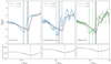 |
Fig. 1. Logarithmic derivative of the average density profiles, and Rspl as function of mass, redshift, and theory of gravity. Upper panels: average profiles of d log ρshell/d log r for the samples of simulated halos in Table 1. The left, middle, and right panels show the average profiles for the low-, intermediate-, and high-mass samples, respectively, at the lowest and highest redshifts of each sample, as listed in the insets. The solid (dash-dotted) curves are the profiles in the ΛCDM (fR4) model. The vertical solid (dash-dotted) thick black lines show the location of Rspl at z = 0 in the ΛCDM (fR4) model. The pair of vertical blue (green) solid and dash-dotted lines shows Rspl at z = 1.0 (z = 0.3) for the ΛCDM and fR4 models, respectively. Bottom panels: the thin solid (dash-dotted) black curves show the radial derivative of the average mass profile in ΛCDM (fR4) at z = 0; the vertical thin solid (dash-dotted) black lines show ςavg of the low-, intermediate-, and high-mass samples at z = 0 in the ΛCDM (fR4) models (Table 2, first row, values in brackets). When extended to the upper panels, these thin solid and dash-dotted black lines cross the average density profiles at dlog ρshell/d log r ≃ −2, as expected from Eq. (1). |
All the simulated average profiles of d log ρshell/d log r show an absolute minimum. Adhikari et al. (2014) associated this feature with Rspl, which roughly corresponds to the first apocenter of the orbits of recently accreted material. We identify Rspl of each halo sample as the point of absolute minimum of the logarithmic derivative of the associated smoothed average density profile ρshell(r). In the upper panels of Fig. 1, each vertical line shows the point of minimum, Rspl, of the logarithmic derivatives of ρshell(r) for the corresponding redshift (color) and theory of gravity (style).
As shown in Table 2, Rspl decreases with increasing redshift at fixed mass, and with increasing mass at fixed redshift. At z ≤ 0.7, at fixed redshift and mass, ΛCDM systematically predicts a smaller Rspl than fR4: From z = 0 to z = 0.7, the relative differences between Rspl in fR4 and ΛCDM is in the range ∼2 − 15% in the low-mass bin, and ∼2 − 35% in the intermediate-mass bin. In the high-mass bin, the same difference increases from ∼5% at z = 0 to ∼55% at z = 0.3. At z ≥ 0.8, the low-mass bin confirms this behavior: Rspl in fR4 is larger than in ΛCDM by ∼2 − 12%. In contrast, in the intermediate-mass bin, at z = 0.8 − 1.0, Rspl in ΛCDM can be ∼22% larger than in fR4.
Radii Rspl and ςavg of the simulated clusters.
A major issue in the use of the d log ρshell/d log r profile is that when it is computed for real clusters from the estimated mass profile, the uncertainty in the ith bin is proportional to ri/(ri + 1 − ri), where ri and ri + 1 are the radii used to compute the numerical derivative of the shell mass density profile, ρshell(r). The uncertainty is thus increasingly large at increasing radius. Furthermore, the dependence of Rspl on ρshell(r) hinders the robust estimation of Rspl due to the scatter caused by the high sensitivity of the logarithmic derivative to rapid changes of ρshell(r) in two adjacent shells. We can overcome these problems by considering, instead of ρshell(r) and Rspl, the radial differential mass profile dM/dr = M′(r) and the radial location, ς, of the minimum of this profile.
Rspl and ς are not equivalent: The condition for Rspl is d[d log ρshell/d log r]/dr = 0, whereas the condition for ς is
 (1)
(1)
The values in brackets in Table 2 show the points of minimum ςavg computed from the radial derivative of the averaged cumulative mass profiles of the halos in each bin. The ςavg appear larger than Rspl: By averaging over all the masses and redshifts, ςavg exceeds Rspl by 43% and 40% in the ΛCDM and fR4 model, respectively. This result agrees with the recent study by García et al. (2021), who reported a ratio of the minimum of r2ξhm, where ξhm is the halo-matter correlation function, and Rspl of ∼1.3. In Fig. 1, the thin solid (dash-dotted) black curves in the bottom panels show the M′ average profiles in ΛCDM (fR4) at z = 0; the thin black vertical solid (dash-dotted) lines show the points of minimum of these curves, namely ςavg in ΛCDM (fR4) at z = 0.
Despite the obvious difference between ςavg and Rspl, these two quantities share remarkable similarities in their dependence on redshift, mass, and gravity model. Table 2 shows that ςavg, similarly to Rspl, decreases with increasing redshift at fixed mass, and with mass at fixed redshift. Moreover, analogously to Rspl, in all the low-mass samples the ςavg in fR4 are larger than in ΛCDM by ∼10%, except in the low-mass sample at z = 1.0, where the ςavg in fR4 is ∼2% smaller than in ΛCDM. Similarly, in all the high-mass samples, the ςavg in fR4 are larger than in ΛCDM by 5 − 55%. In the intermediate-mass bin, the similarity with Rspl also holds globally: At z ≤ 0.4, the ςavg in fR4 are larger than in ΛCDM by 5 − 35%. At higher redshifts, this hierarchy can be inverted, with ςavg in ΛCDM larger up to 29% than in fR4.
We assessed how well ς can distinguish between the ΛCDM and fR4 models through its dependence on redshift and mass. To do this, in addition to ςavg extracted from the average mass profiles and discussed above, we used a different estimate of ς extracted from the individual mass profiles. In the simulations, the M′(r) profiles are less sensitive to sudden mass differences caused by random variations in the number of dark matter particles in two adjacent shells. We are thus able to exploit the ςs of the individual halos in our analysis. More precisely, for each redshift and mass bin, we computed the cumulative radial mass profiles of all the halos. The profiles were obtained by progressively adding from the center the mass of 200 adjacent spherical shells with logarithmically spaced outer cluster-centric radii spanning the range (0.1, 10)R200c. For each halo, we computed the corresponding radial derivative of the mass profile.
In Fig. 2, the upper, middle, and bottom panels show the median radial differential mass profiles M′(r) of the low-, intermediate-, and high-mass samples of Table 1, respectively, with their 68th percentile ranges. The solid (dash-dotted) curves are for the ΛCDM (fR4) samples: for each sample, the value of the corresponding curve at each radial bin ri is the median of the set of the individual M′(ri) of all the halos in the sample; each point of these curves is determined by a number of data equal to the size of the corresponding sample (columns “size” in Table 1).
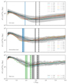 |
Fig. 2. Median differential radial mass profiles of the samples of the simulated halos in Table 1. The top, middle, and bottom panels show the results for the low-, intermediate-, and high-mass samples, respectively. The solid (dash-dotted) curves are the median profiles for the ΛCDM (fR4) halos. The profiles of the halos at different redshifts are shown with different colors, as listed in the insets. The shaded gray areas show the 68th percentile range of the distributions of the profiles of the individual halos at z = 0 in the ΛCDM model. The spreads of the profiles at the other redshifts and in the fR4 model are comparable. The vertical thick solid (dash-dotted) black line shows the median radius ς at z = 0 in the ΛCDM (fR4) model. The vertical thick blue (green) lines show ς for the profiles at z = 1.0 (z = 0.3): the solid and dash-dotted lines show the ΛCDM and fR4 models, respectively. The dash-dotted blue line in the upper panel is overplotted on the solid blue line. The vertical stripes indicate the error bands of the median ςs. |
We identified the final ς of each mass and redshift sample as the median of the set of all the ςs of the individual halos in the sample. The ς of each individual halo is the minimum of the corresponding profile M′(r) beyond 0.5R200c. This choice avoids possible inconsistencies caused by high fluctuations in the inner region of the halo. In Fig. 2, the solid (dash-dotted) vertical lines show the value of ς in ΛCDM (fR4) at the lowest and highest redshift of the three mass bins. In general, the position of ς does not coincide with the minimum of the corresponding median profile in Fig. 2 because we did not select ς at the minimum of the median profile of the individual halos, but as the median of the ςs of the individual halos. Table 3 lists the median ς of the individual differential mass profiles for the samples listed in Table 1. We also provide an estimate of the error of the median with the difference between the median and the corresponding 16th percentile, and the difference between the median and the 84th percentile value divided by the square root of the sample size. We also display the relative differences of ς in ΛCDM and fR4. Figure 3 shows ς as a function of redshift and mass in ΛCDM and fR4.
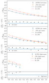 |
Fig. 3. Medians and associated errors of ς as a function of redshift in ΛCDM (blue points) and fR4 (orange points) for the low- (top panel), intermediate- (middle panel), and high-mass (bottom panel) samples. We applied small redshift offsets to the fR4 points to facilitate comparison. The black (red) lines are the fits of Eq. (4) to the ΛCDM (fR4) points: specifically, the curves are the result of a spline interpolation of the values of ς (11 for the low- and intermediate-mass bin, 4 for the high-mass bin) resulting from Eq. (4) using the redshift, mass, and mass accretion rate of each simulated bin (Table 1). In each panel, the lower plot shows the differences of the median ςs in ΛCDM and fR4 relative to the ΛCDM value. |
ς of the simulated clusters.
These new estimates of ς confirm the previous trends shown by ςavg, but the results are less prone to large scatter: ς decreases with increasing redshift and mass; furthermore, at fixed redshift and mass, ΛCDM generally predicts a smaller ς than fR4. As shown in Table 3, in the low- and high-mass bins, ς is systematically larger in fR4 than in ΛCDM: In the low-mass bin, the relative difference decreases with redshift from ∼12% at z = 0 to 0% at z = 1; in the high-mass bin, the ςs in fR4 are increasingly larger than in ΛCDM as redshift increases, from ∼19% at z = 0 to ∼25% at z = 0.3. In the intermediate-mass bin, ς is systematically larger in fR4 at redshift z ∼ 0 − 0.5, where the relative difference decreases from ∼12% to ∼5%. In this mass bin, similarly to Rspl (Table 2), ΛCDM can present larger ςs than fR4 at z > 0.5.
3.2. Dependence of ς on redshift, MAR, and the theory of gravity
In the previous section, we showed that ς, analogously to Rspl, is sensitive to the redshift and the mass of the cluster, and that it can be up to 25% larger in fR4 than in ΛCDM (Table 3). Mass and MAR are tightly correlated (Diemer & Kravtsov 2014; Pizzardo et al. 2021). Our findings therefore agree with previous results showing that Rspl is correlated with redshift and MAR (More et al. 2015). In this section, we model the behavior of ς with z and MAR as independent variables, and we investigate whether ς can distinguish between ΛCDM and fR4.
Our definition of the MAR can be easily extended to real clusters because it does not rely on the merger history of the halos, as is usually adopted in investigations based on N-body simulations. We considered the procedure by Pizzardo et al. (2021, 2022), who measured the MAR of ∼500 real clusters of galaxies. The recipe is based on the assumption that the infall of new material onto the clusters is described by the spherical accretion model (De Boni et al. 2016). Namely, in the infall time tinf, a cluster accretes all the material within a spherical shell, centered on the cluster center, with inner radius Ri and thickness Δs = δsRi. The quantity δs is derived from the equation of motion of the infalling mass with initial velocity vinf and constant acceleration −GM(< Ri)/(Ri + δsRi/2)2,
 (2)
(2)
where M(< Ri) is the mass of the cluster within Ri, and G is the gravitational constant. Here, according to De Boni et al. (2016) and Pizzardo et al. (2021, 2022), we fixed tinf = 1 Gyr and Ri = 2R200c, whereas for the infall velocity, vinf, we relied on the radial velocity profiles of the simulated halos of DUSTGRAIN in the two theories of gravity. For a sample of simulated clusters, vinf is the minimum velocity of the median radial velocity profile in the range [2, 2.5]R200c of the sample, whereas for a sample of real clusters, vinf results from suitable interpolations of the simulated samples (see Pizzardo et al. 2021, 2022, for further details). When the mass of the infalling shell, Mshell, is known, the MAR is estimated with the equation
 (3)
(3)
We computed the MARs of all the halos in the samples of Table 1. This table lists the median MAR of each sample with their corresponding 68th percentile range. In Fig. 4, the open circles show the median MARs of the 26 ΛCDM samples as a function of the median mass of the sample, color-coded by redshift. By considering the merging history of simulated CDM halos, Diemer et al. (2017) proposed an accretion law that we computed at our 11 simulated redshifts and show with the curves in Fig. 4. The agreement between this law and our estimates shows that the MARs of galaxy clusters estimated with our recipe, which can be applied to real clusters, are consistent with the MARs derived from the merger trees, which remain inaccessible to observations. The estimated MARs of the CIRS and HeCS clusters (Pizzardo et al. 2021, squares in Fig. 4) and of the HectoMAP clusters (Pizzardo et al. 2022, diamonds in Fig. 4) agree with the theoretical expectations of ΛCDM within the uncertainties. Both M200c and MAR are estimated from the same caustic mass profile, hence their errors are not independent. However, the error of the caustic mass profile at a given radius is determined by the number and the distribution of the galaxies within the spherical shell centered at this radius, and M200c and MAR are estimated at well-separated radii. Therefore, we can assume that the errors on these quantities are independent, and we obtain a roughly correct estimate of the expected uncertainty ranges (error bars in Fig. 4).
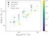 |
Fig. 4. MAR as a function of the cluster mass M200c in the simulations and the MAR of the CIRS, HeCS, and HectoMAP clusters. The open circles show the median MARs of the 26 ΛCDM samples of Table 1, color-coded by redshift. The colored curves are the relation of Diemer et al. (2017) computed at the 11 redshifts of our simulated samples. The squares and the diamonds with error bars show the MAR estimates with their uncertainties of the stacked clusters of the CIRS and HeCS (Pizzardo et al. 2021) and HectoMAP clusters (Pizzardo et al. 2022), respectively. |
For each of the two sets of simulations, we fit the 26 points in the four-dimensional space (ς,z, MAR, M200c) with the relation
![Mathematical equation: $$ \begin{aligned} \frac{\varsigma }{R_{200c}}(z, \text{ MAR}, M_{200c}) = a \left[1 + b\, \Omega _{\rm M}(z)\right] \left[1 + c\, \exp \left(-\frac{\Gamma _{\rm dyn}}{d}\right) \right], \end{aligned} $$](/articles/aa/full_html/2024/02/aa44448-22/aa44448-22-eq180.gif) (4)
(4)
where ΩM(z) = ΩM(1 + z)3/[ΩM(1 + z)3 + ΩΛ], Γdyn is the dynamical MAR  , with
  the scale factor, and a, b, c, and d are four free parameters. Figure 4 proves that the difference between the Mvirs at two different epochs is comparable with the difference between the masses of the infalling shell that we adopted in our definition of MAR. With an obvious change in the variables, we can therefore express the dynamical accretion rate as Γdyn ≈ [𝒦(t, ΩM, H0)/M200c] (dM/dt), with dM/dt ≡ MAR3. Table 1 reports Γdyn for each cluster sample. Equation (4) was proposed by More et al. (2015) to model Rspl rather than ς. The similar behavior of these two quantities with redshift, MAR, and mass leads us to heuristically use the same functional form for ς, however. We also kept ΩM(z) in the form of ΛCDM in the fit to the fR4 data in order to direct any difference to the four fitting parameters a, b, c, and d. We fit the median points with a nonlinear least-squares Marquardt–Levenberg algorithm by weighting the points with the inverse of their variance (Table 3). The values of the coefficients are reported in Table 4.
Table 4 shows that the ΛCDM fit is robust. The parameter b, which controls the dependence of ς on redshift, is constrained with a relative uncertainty of ∼10%; the parameters c and d, which control the dependence of ς on the logarithmic MAR, are constrained with uncertainties of ∼45 − 47%. This result shows that in ΛCDM the dependence of ς on redshift and MAR are statistically significant and are similar to those expected for Rspl. The fR4 fit is less strongly constrained: Except for the parameter b with a ∼10% uncertainty, the remaining three parameters are affected by uncertainties of ∼100% or larger. However, the model of Eq. (4) was only proposed to fit the relation in the ΛCDM universe. The large uncertainties on the parameters for the fR4 fit can thus simply suggest that Eq. (4) is less adequate for this gravity model.
The absolute value of the relative differences between the fit and the actual values is ∼4.2% and ∼3.5% for the ΛCDM and the fR4 samples on average, respectively. Figure 3 shows examples of these fits in the ς − z plane. Figure 5 shows projections of the fits on the ς–MAR plane at three different redshifts. The correlation of ς with redshift and MAR is confirmed by the Kendall test, which returns a tight correlation with a p-value 10−5 for the relation ς − z and for the relation ς–MAR.
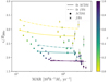 |
Fig. 5. ς as a function of MAR, color-coded by redshift. The circles and crosses show the median values of the ΛCDM and fR4 samples, respectively. The solid (dash-dotted) curves are the fits of Eq. (4) to the ΛCDM (fR4) data at three redshifts. From top to bottom, z = 0.0, 0.5, and 1.0. At fixed redshift, ς decreases with increasing MAR; at fixed MAR, ς decreases as the redshift increases. |
As expected, the fits show that the difference between the ΛCDM and fR4 models is larger at low redshifts, independently of the MAR. The difference steadily decreases with increasing redshift: consequently, because at low redshift ς is higher in fR4 than in ΛCDM, the fits in the (ς,z) plane at fixed MAR (Fig. 3) show steeper profiles in fR4 than in ΛCDM.
We now quantitatively assess to which extent ς can distinguish between ΛCDM and fR4. We applied the median test to each of our 26 ΛCDM–fR4 pairs of the distributions of the individual ς at equal redshift and mass bin. This test counts the number of elements of the two distributions that are either larger or smaller than the grand median of the two samples. Based on a Pearson χ-squared test, the test assigns a p-value to the null-hypothesis that the samples are drawn from the same distribution. Generally, the fR4 sample is more densely populated than the corresponding sample in ΛCDM (see Table 1). To perform the test on samples with the same number of halos, we therefore randomly undersampled each fR4 sample to the number of halos in the corresponding ΛCDM sample. The results of the median test are shown in Fig. 6: the blue points in the upper panel are for the low-mass samples, whereas the orange and green points in the lower panel are for the intermediate- and high-mass samples, respectively.
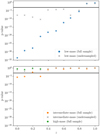 |
Fig. 6. p-values of the median test to distinguish the two theories of gravity performed on the samples of ςs of the simulated clusters in Table 1. Top panel: blue points show the p-values of the test on the full samples of ςs in the low-mass bin, and the gray crosses show the p-values of the test performed by undersampling all the low-mass samples to 646 halos. Bottom panel: orange and green points show the p-values of the test on the full samples in the intermediate- and high-mass bin, respectively; the gray crosses show the p-values of the test performed by undersampling the intermediate-mass samples to 11 halos. In both panels, the horizontal lines denote p = 10−3. |
We took p = 10−3 as the upper limit to conclude that the two theories of gravity can be distinguished: Values below this limit are evidence at a significance level higher than 3σ that the two samples are drawn from different populations. Figure 6 shows that the low-mass samples can generally distinguish between the two models in the redshift range z ∼ 0 − 0.8. The samples at the lowest redshifts show extremely strong evidence that gravity is modified (p ≈ 10−30). In contrast, only 3 of 11 intermediate-mass samples show some evidence of modified gravity, and none of the high-mass samples is able to do so.
The progressively weaker discerning power of the median test in the low-mass samples as redshift increases is due to the intrinsic degeneracy of fR4 and ΛCDM at high redshift. We illustrate in Appendix A that the main differences between the two models are more evident at late times. This conclusion is also supported by the steady decrease in the relative difference between the ςs of the two models as redshift increases (see Table 3). In contrast, the largest part of the intermediate- and high-mass samples shows p > 10−3 even at low redshift, where the relative difference between the values of ς is similar to or larger than for the low-mass halos (Table 3). The reason for this behavior is the small number of halos in these mass samples and not the intrinsic similarity of the models.
To test the effect of poor sampling, we considered for the low- and intermediate-mass bins the corresponding sample with the lowest number of halos, regardless of redshift and model: Table 1 shows that the smallest samples are the ΛCDM samples at z = 1.0, with 646 and 11 halos for the low- and intermediate-mass bins, respectively. We therefore performed a median test in which we randomly undersampled all the samples of the low- and intermediate-mass bins to 646 and 11 halos, respectively.
The results are shown by the gray crosses in Fig. 6. In the low-mass bin, the undersampling increases the p-value of the median test for the samples at z ∼ 0 − 0.8; furthermore, the increment of the p-value decreases with redshift because the higher the redshift, the fewer halos are removed. Nevertheless, at z < 0.9, although they are substantially reduced, the p-values remain below 10−3.
The important result of this test is the minimum size of the sample required to distinguish between the two theories of gravity: As long as the sample size is ≳400, the distinguishing power remains substantially unaffected. Therefore, in the low-mass bin, the loss of significance of the median test to distinguish the theory of gravity at high redshifts, z ∼ 0.9 − 1.0, is caused by the intrinsic degeneracy between fR4 and ΛCDM at these early times and not by the sample size. Conversely, the failure of the distinguishing ability of ς in the intermediate- and high-mass bins is caused by the small halo samples. As long as the sample size is ∼230 − 400, as in the first four redshift bins of the full intermediate-mass bin, the distinguishing power is still present. With smaller sample sizes, however, the p-values are aligned to the results of the intermediate-mass full samples at z ≳ 0.4, and of the high-mass full sample, where we have ∼10 − 150 halos.
4. Discussion
We have investigated the radial location, ς, of the minimum of the radial differential mass profile, M′(r), of simulated galaxy clusters halos. Although not equivalent, we show that ς shares similarities with the splashback radius, Rspl. We show that ς can distinguish among different gravity models. We investigated General Relativity, with the standard ΛCDM model, and f(R) gravity. Our work strengthens the hypothesis that galaxy clusters might be used as cosmological probes. In particular, we showed that the outskirts of clusters promise to effectively complement more traditional cluster-based cosmological tests, such as cluster counts and the gas fraction (see Cataneo & Rapetti 2020, for a review of the tests of gravity with galaxy clusters).
Like Rspl, ς can be located directly from the mass profiles of galaxy clusters. Most works that searched for Rspl relied on the projected galaxy number density profile or on the projected luminosity profile. These quantities are tightly related and are good proxies of the three-dimensional matter density profile in general (Carlberg et al. 1997; Rines et al. 2003, 2004; Rines & Diaferio 2006; Rines et al. 2013). However, many studies have pointed out that the galaxy number density and luminosity profiles are not directly proportional to each other (e.g., Proctor et al. 2015). In addition, their correlation is sensitive to the cluster mass and to the selection function (Mulroy et al. 2014). Moreover, if the galaxy density is constrained by photometrically detected clusters, projection effects and member mismatch become increasingly relevant in the outer regions (e.g., More et al. 2016; Baxter et al. 2017; Shin et al. 2019). The use of the mass profile to detect Rspl or ς is clearly preferred because the definitions of these quantities are based on the mass profile that is measured in N-body simulations.
Furthermore, the detection of ς from mass profiles is prone to smaller fluctuations than the detection of Rspl because the radial derivative M′(r) is much less noisy than the logarithmic slope of the matter density. For this reason, unlike Rspl, ς can be located in individual clusters if the mass profile is accurately estimated up to ∼3 − 4R200.
Using ς as a probe of the theory of gravity requires an unbiased estimate of hundreds of cluster mass profiles up to large cluster-centric radii with high-precision and accuracy. Weak gravitational lensing (Bartelmann 2010; Hoekstra et al. 2013; Umetsu 2020) and the caustic technique (Diaferio & Geller 1997; Diaferio 1999; Serra et al. 2011) are the only methods that can be reliably used beyond the inner region of clusters, where dynamical equilibrium does not hold.
The current cluster samples do not allow us to robustly locate ς and to statistically use it as a probe of the theory of gravity. However, future facilities such as the VRO (Ivezić et al. 2019) and the Euclid mission (Laureijs et al. 2011; Sartoris et al. 2016) will provide weak-lensing mass measurements of thousands of clusters. Powerful spectrographs such as the multi-object William Herschel Telescope Enhanced Area Velocity Explorer spectrograph on the WHT (WEAVE, Balcells et al. 2010; Dalton et al. 2012, 2014; Dalton 2016) will explore the infall regions of galaxy clusters and provide dense spectroscopic surveys out to radii ≲5R200c of more than 100 clusters at redshift ≲0.5. Planned observations with the Prime Focus Spectrograph on Subaru (PFS, Tamura et al. 2016) and the Maunakea Spectroscopic Explorer on the CFHT (MSE, Marshall et al. 2019) will provide spectroscopic redshifts of hundreds to thousands of galaxy cluster members for thousands of individual clusters at z ≲ 0.6. These surveys will allow a precise and unbiased determination of ς from weak lensing and the caustic technique.
These future observations will enable synergies between photometric and spectroscopic techniques. These synergies will be crucial for promoting ς as a probe of gravity. At cluster-centric distances of about ς, a misidentification of background galaxies and large-scale structure can severely bias weak-lensing mass profiles obtained from photometric redshifts (Hoekstra 2003; Hoekstra et al. 2011; Becker & Kravtsov 2011; Sommer et al. 2022). The caustic technique provides unbiased mass profiles on average, but the scatter is relevant (Serra et al. 2011; Pizzardo et al. 2023a). The joint use of these two techniques could take advantage of the respective strengths, and it would be crucial to obtain exquisitely robust mass estimates up to large cluster-centric distances (e.g., Dell’Antonio et al. 2020).
As a cautionary note about our analysis presented in this work, we recall that the ΛCDM and fR4 runs of the DUSTGRAIN simulations that we used here were normalized at the CMB epoch. Therefore, their power-spectrum normalization at z = 0, σ8 was 0.847 and 0.967 for the two models (Sect. 2.1). To show that our results are not affected by these different values of σ8, we compared the median MARs at z = 0 of our low- and high-mass ΛCDM samples with the median MARs estimated by Pizzardo et al. (2021, 2022) in the ΛCDM L-CoDECS N-body simulation of Baldi (2012), which has σ8 = 0.809. Despite the lower σ8, we find that the MARs in the L-CoDECS simulation are ∼14% and ∼3% larger than the MARs of our DUSTGRAIN samples for the low- and the high-mass bin, respectively. Moreover, ς is ∼4.5% smaller in the DUSTGRAIN clusters than in the L-CoDECS simulations for both the low- and high-mass bin. In addition, in DUSTGRAIN, σ8, ΛCDM < σ8, fR4, which means that if ς were inversely proportional to σ8, we should expect ςs larger in ΛCDM than in fR4 at fixed redshift and mass. This expectation is the opposite of the results from the simulations (Table 3). Hence, the behavior of ς does not appear to be correlated with σ8, and therefore, the differences between the models that we find here are mainly driven by the different theory of gravity.
One might expect that the outer regions of clusters smoothly approach the uniform cosmic background and that this background contributes to the mass profile of the clusters. However, the distribution of matter around both simulated (e.g., Gao et al. 2004; van den Bosch et al. 2005; Cornwell et al. 2023, 2024) and real clusters (e.g., Beers et al. 1983; Dressler & Shectman 1988; Martínez et al. 2016; Sarron et al. 2019) is inhomogeneous, with filaments, groups of galaxies, and low-density regions. Therefore, we did not subtract the contribution of a uniform background from the mass profile the clusters in our analysis (see Sect. 3.1). Nevertheless, we verified that the effect of subtracting a uniform background with density ΩMρc from the mass profiles has a negligible effect on our results: The radii ς at which the minimum of the radial derivative of the cluster mass profile occurs are ∼10% larger on average than the ςs from the profiles without subtraction. More importantly, the correlations between ς, redshift, and MAR are preserved at similar significance levels.
We showed that extended ranges of mass and redshift are critical to avoid possible degeneracies between the models. Thus, our analysis pointed out the importance of further efforts toward the realization of simulations of large cosmological volumes in modified gravity. Larger samples that include the most massive clusters can help us to establish the correlation between ς and MAR with more significance because these samples will allow us to stack clusters based on mass and to probe a more extended range of MARs at fixed redshift. Furthermore, the most massive clusters, with a mass ∼1015 h−1 M⊙, are expected to provide the most robust evidence of possible deviations from the standard scenario because these clusters probe the upper tail of the mass function, which is extremely sensitive to the cosmological model (Bardeen et al. 1986; White 2002; Courtin et al. 2011; Cui et al. 2012; Giocoli et al. 2018), and because they are the easiest objects to detect observationally. In Sect. 3 we showed that in the high-mass samples of simulated clusters, we observe the largest discrepancy between the values of ς in the two models of gravity (Table 3). Nevertheless, the larger sizes of the low- and intermediate-mass samples, compared to the high-mass sample, enable the best distinction between the two models of gravity (Sect. 3.2). On the one hand, large simulated volumes can therefore provide samples with an adequate size for a solid test bench based on which the performance of ς as a gravitational probe can be investigated. On the other hand, low- and intermediate-mass clusters, with ∼1 − 5 × 10¹⁴ h−1 M⊙, can already provide observed samples that are sufficiently large to yield tight constraints on the theory of gravity.
5. Conclusion
We performed the first assessment of the ability of the radial location, ς, of the minimum of the differential radial mass profiles, M′(r), of clusters of galaxies to distinguish between two different models of gravity, General Relativity, with the ΛCDM model, and f(R). We investigated the behavior of ς in a wide range of masses, M200c ∼ (0.9 − 11)×1014 h−1 M⊙, and redshift, 0.0 ≤ z ≤ 1.0. We explored the dependence of ς on redshift and MAR in the two models. We also showed that ς has a similar redshift, mass, and MAR dependence as the splashback radius.
We used the DUSTGRAIN N-body simulations (Giocoli et al. 2018). We considered the ΛCDM run and the Hu-Sawicki f(R) (Hu & Sawicki 2007) run with scalaron fR = −1 × 10⁻⁴ (fR4). By means of ∼21 000 and ∼28 000 dark matter halos in ΛCDM and fR4, respectively, arranged into three mass bins and 11 redshift bins, we showed that in both models ς decreases with increasing redshift at fixed mass and decreases with increasing mass (or equivalently, MAR) at fixed redshift. Specifically, in the ΛCDM model, ς decreases from ∼3R200c to ∼2R200c when z increases from 0 to 1. At z ∼ 0.1, ς decreases from 2.8R200c to ∼2.5R200c when the MAR increases from ∼104 h−1 M⊙ yr−1 to ∼2 × 10⁵ h−1 M⊙ yr−1. We computed the MAR with the recipe presented in Pizzardo et al. (2021, 2022), which, we demonstrated, agrees with results based on the merger trees of dark matter halos (Diemer et al. 2017). The behavior of ς in fR4 is similar to that of the ΛCDM, but at low redshifts, ς in fR4 is ∼15% larger on average than in ΛCDM, whereas at higher redshifts (z ∼ 0.8 − 1.0) the ςs of the two models overlap. In ΛCDM, the correlations of ς with redshift and MAR agree with the correlations expected for the splashback radius (Diemer & Kravtsov 2014; Adhikari et al. 2014; Deason et al. 2021; O’Neil et al. 2021; Baxter et al. 2021; Dacunha et al. 2022).
By using the median test, we find that when the dark matter halos with mass ∼1014 h−1 M⊙ at z ≤ 0.8 are considered, ς can distinguish between the two theories of gravity with high significance, with a p-value ≲10−5. At z ≤ 0.5, the same halos give a p-value ≲10−15. At the highest redshift, ΛCDM and fR4 are degenerate, and ς cannot distinguish between the two models. Conversely, the number of halos with mass ∼1015 h−1 M⊙ is too small to distinguish between the two models at any redshift: We showed that obtaining a p-value ≲10−5 requires ≳400 halos.
Developing the full potential of the ς radius as a gravity probe thus requires further observational and computational efforts. New facilities such as the Vera Rubin Observatory (Ivezić et al. 2019) and Euclid (Laureijs et al. 2011; Sartoris et al. 2016) will provide extended weak-lensing mass profiles for thousands of clusters up to z ∼ 2. Large dense surveys obtained with advanced spectrographs on large telescopes such as WEAVE (Balcells et al. 2010; Dalton et al. 2012, 2014; Dalton 2016), PFS (Tamura et al. 2016), and eventually, MSE (Marshall et al. 2019) will provide dense spectroscopic surveys of a tremendous number of clusters up to z ∼ 0.5 that will complement the photometry. Weak gravitational lensing mass profiles estimated with sophisticated mass reconstruction methods (e.g., Umetsu et al. 2011; Umetsu 2013) combined with the caustic mass profiles (Diaferio & Geller 1997; Diaferio 1999; Serra et al. 2011; Pizzardo et al. 2023a) will improve the accuracy and the precision of the mass profiles at large distance from the cluster center. Larger simulated volumes will allow the identification of larger sets of the most massive halos, paving the way to tighter tests of structure formation models.
In the following, R200c will denote the radius within which the mean density equals 200 times the critical density ρc. It is a common proxy of the virial radius (Bryan & Norman 1998).
The different values of σ8 in the two simulations do not affect our results, as discussed in Sect. 4.
𝒦 transforms the time coordinates from the scale factor to cosmic time:  .
.
Acknowledgments
We sincerely thank the referee for her/his insightful comments that greatly improved the quality of the paper. We thank Marco Baldi for providing snapshots of the ΛCDM and fR4 runs of the DUSTGRAIN N-body simulation. We thank Margaret Geller, Jubee Sohn, and Benedikt Diemer for numerous stimulating discussions. The graduate-student fellowship of M.P. was supported by the Italian Ministry of Education, University and Research (MIUR) under the Departments of Excellence grant L.232/2016. M.P. acknowledges the support of the Canada Research Chair Program and the Natural Sciences and Engineering Research Council of Canada (NSERC, funding reference number RGPIN-2018-05425). We also acknowledge partial support from the INFN grant InDark. This research has made use of NASA’s Astrophysics Data System Bibliographic Services.
References
- Achitouv, I., Wagner, C., Weller, J., & Rasera, Y. 2014, J. Cosmol. Astropart. Phys., 2014, 077 [CrossRef] [Google Scholar]
- Ade, P. A., Aghanim, N., Arnaud, M., et al. 2016, A&A, 594, A13 [NASA ADS] [CrossRef] [EDP Sciences] [Google Scholar]
- Adhikari, S., Dalal, N., & Chamberlain, R. T. 2014, J. Cosmol. Astropart. Phys., 11, 019 [CrossRef] [Google Scholar]
- Adhikari, S., Sakstein, J., Jain, B., Dalal, N., & Li, B. 2018, J. Cosmol. Astropart. Phys., 2018, 033 [CrossRef] [Google Scholar]
- Armitage, T. J., Barnes, D. J., Kay, S. T., et al. 2018, MNRAS, 474, 3746 [NASA ADS] [CrossRef] [Google Scholar]
- Balcells, M., Benn, C. R., Carter, D., et al. 2010, in Ground-based and Airborne Instrumentation for Astronomy III, eds. I. S. McLean, S. K. Ramsay, & H. Takami, SPIE Conf. Ser., 7735, 77357G [NASA ADS] [Google Scholar]
- Baldi, M. 2012, MNRAS, 422, 1028 [NASA ADS] [CrossRef] [Google Scholar]
- Banerjee, A., Adhikari, S., Dalal, N., More, S., & Kravtsov, A. 2020, J. Cosmol. Astropart. Phys., 2020, 024 [CrossRef] [Google Scholar]
- Bardeen, J. M., Bond, J. R., Kaiser, N., & Szalay, A. S. 1986, ApJ, 304, 15 [Google Scholar]
- Bartelmann, M. 2010, Class. Quant. Grav., 27, 233001 [CrossRef] [Google Scholar]
- Baxter, E., Chang, C., Jain, B., et al. 2017, ApJ, 841, 18 [NASA ADS] [CrossRef] [Google Scholar]
- Baxter, E. J., Adhikari, S., Vega-Ferrero, J., et al. 2021, MNRAS, 508, 1777 [NASA ADS] [CrossRef] [Google Scholar]
- Becker, M. R., & Kravtsov, A. V. 2011, ApJ, 740, 25 [NASA ADS] [CrossRef] [Google Scholar]
- Beers, T. C., Huchra, J. P., & Geller, M. J. 1983, ApJ, 264, 356 [NASA ADS] [CrossRef] [Google Scholar]
- Bianconi, M., Buscicchio, R., Smith, G. P., et al. 2021, ApJ, 911, 136 [Google Scholar]
- Bower, R. G. 1991, MNRAS, 248, 332 [NASA ADS] [CrossRef] [Google Scholar]
- Bryan, G. L., & Norman, M. L. 1998, ApJ, 495, 80 [NASA ADS] [CrossRef] [Google Scholar]
- Buchdahl, H. A. 1970, MNRAS, 150, 1 [NASA ADS] [Google Scholar]
- Carlberg, R., Yee, H., Ellingson, E., et al. 1997, ApJ, 485, L13 [NASA ADS] [CrossRef] [Google Scholar]
- Cataneo, M., & Rapetti, D. 2020, MODIFIED GRAVITY: Progresses andOutlook of Theories, Numerical Techniques and Observational Tests (World Scientific), 143 [Google Scholar]
- Chang, C., Baxter, E., Jain, B., et al. 2018, ApJ, 864, 83 [NASA ADS] [CrossRef] [Google Scholar]
- Contigiani, O., Vardanyan, V., & Silvestri, A. 2019, Phys. Rev. D, 99, 064030 [NASA ADS] [CrossRef] [Google Scholar]
- Corasaniti, P. S., & Achitouv, I. 2011, Phys. Rev. Lett., 106, 241302 [NASA ADS] [CrossRef] [Google Scholar]
- Cornwell, D. J., Aragón-Salamanca, A., Kuchner, U., et al. 2023, MNRAS, 524, 2148 [NASA ADS] [CrossRef] [Google Scholar]
- Cornwell, D. J., Kuchner, U., Gray, M. E., et al. 2024, MNRAS, 527, 23 [Google Scholar]
- Courtin, J., Rasera, Y., Alimi, J.-M., et al. 2011, MNRAS, 410, 1911 [NASA ADS] [Google Scholar]
- Cui, W., Baldi, M., & Borgani, S. 2012, MNRAS, 424, 993 [NASA ADS] [CrossRef] [Google Scholar]
- Dacunha, T., Belyakov, M., Adhikari, S., et al. 2022, MNRAS, 512, 4378 [NASA ADS] [CrossRef] [Google Scholar]
- Dalton, G. 2016, in Multi-Object Spectroscopy in the Next Decade: Big Questions, Large Surveys, and Wide Fields, eds. I. Skillen, M. Balcells, & S. Trager, ASP Conf. Ser., 507, 97 [Google Scholar]
- Dalton, G., Trager, S., & Abrams, D. C. 2014, in Ground-based and Airborne Instrumentation for Astronomy V, eds. S. K. Ramsay, I. S. McLean, & H. Takami, SPIE Conf. Ser., 9147, 91470L [Google Scholar]
- Dalton, G., Trager, S. C., Abrams, D. C., et al. 2012, in Ground-based and Airborne Instrumentation for Astronomy IV, SPIE, 8446, 220 [Google Scholar]
- Davis, M., Efstathiou, G., Frenk, C. S., & White, S. D. M. 1985, ApJ, 292, 371 [Google Scholar]
- De Boni, C., Serra, A. L., Diaferio, A., Giocoli, C., & Baldi, M. 2016, ApJ, 818, 188 [NASA ADS] [CrossRef] [Google Scholar]
- De Simone, A., Maggiore, M., & Riotto, A. 2011, MNRAS, 418, 2403 [CrossRef] [Google Scholar]
- Deason, A. J., Oman, K. A., Fattahi, A., et al. 2021, MNRAS, 500, 4181 [Google Scholar]
- Dell’Antonio, I., Sohn, J., Geller, M. J., McCleary, J., & von der Linden, A. 2020, ApJ, 903, 64 [CrossRef] [Google Scholar]
- Diaferio, A. 1999, MNRAS, 309, 610 [CrossRef] [Google Scholar]
- Diaferio, A. 2004, Outskirts of Galaxy Clusters (IAU C195): Intense Life in the Suburbs (Cambridge: Cambridge University Press), 195 [Google Scholar]
- Diaferio, A., & Geller, M. J. 1997, ApJ, 481, 633 [NASA ADS] [CrossRef] [Google Scholar]
- Diemand, J., Moore, B., & Stadel, J. 2004, MNRAS, 352, 535 [NASA ADS] [CrossRef] [Google Scholar]
- Diemer, B. 2020, ApJ, 903, 87 [NASA ADS] [CrossRef] [Google Scholar]
- Diemer, B. 2021, ApJ, 909, 112 [NASA ADS] [CrossRef] [Google Scholar]
- Diemer, B., & Kravtsov, A. V. 2014, ApJ, 789, 1 [NASA ADS] [CrossRef] [Google Scholar]
- Diemer, B., Mansfield, P., Kravtsov, A. V., & More, S. 2017, ApJ, 843, 140 [NASA ADS] [CrossRef] [Google Scholar]
- Dressler, A., & Shectman, S. A. 1988, AJ, 95, 985 [Google Scholar]
- Fong, M., & Han, J. 2021, MNRAS, 503, 4250 [NASA ADS] [CrossRef] [Google Scholar]
- Gao, L., White, S. D. M., Jenkins, A., Stoehr, F., & Springel, V. 2004, MNRAS, 355, 819 [Google Scholar]
- García, R., Rozo, E., Becker, M. R., & More, S. 2021, MNRAS, 505, 1195 [CrossRef] [Google Scholar]
- Giocoli, C., Baldi, M., & Moscardini, L. 2018, MNRAS, 481, 2813 [Google Scholar]
- Gonzalez, A. H., George, T., Connor, T., et al. 2021, MNRAS, 507, 963 [NASA ADS] [CrossRef] [Google Scholar]
- Hellwing, W. A., Schaller, M., Frenk, C. S., et al. 2016, MNRAS, 461, L11 [NASA ADS] [CrossRef] [Google Scholar]
- Hoekstra, H. 2003, MNRAS, 339, 1155 [NASA ADS] [CrossRef] [Google Scholar]
- Hoekstra, H., Hartlap, J., Hilbert, S., & van Uitert, E. 2011, MNRAS, 412, 2095 [NASA ADS] [CrossRef] [Google Scholar]
- Hoekstra, H., Bartelmann, M., Dahle, H., et al. 2013, Space. Sci. Rev., 177, 75 [NASA ADS] [CrossRef] [Google Scholar]
- Hu, W., & Sawicki, I. 2007, Phys. Rev. D, 76, 064004 [CrossRef] [Google Scholar]
- Ivezić, Ž., Kahn, S. M., Tyson, J. A., et al. 2019, ApJ, 873, 111 [Google Scholar]
- Lacey, C., & Cole, S. 1993, MNRAS, 262, 627 [NASA ADS] [CrossRef] [Google Scholar]
- Lau, E. T., Nagai, D., Avestruz, C., Nelson, K., & Vikhlinin, A. 2015, ApJ, 806, 68 [NASA ADS] [CrossRef] [Google Scholar]
- Laureijs, R., Amiaux, J., Arduini, S., et al. 2011, ArXiv e-prints [arXiv:1110.3193] [Google Scholar]
- Marshall, J., Bolton, A., Bullock, J., et al. 2019, BAAS, 51, 126 [Google Scholar]
- Martínez, H. J., Muriel, H., & Coenda, V. 2016, MNRAS, 455, 127 [CrossRef] [Google Scholar]
- More, S., Diemer, B., & Kravtsov, A. V. 2015, ApJ, 810, 36 [Google Scholar]
- More, S., Miyatake, H., Takada, M., et al. 2016, ApJ, 825, 39 [NASA ADS] [CrossRef] [Google Scholar]
- Mulroy, S. L., Smith, G. P., Haines, C. P., et al. 2014, MNRAS, 443, 3309 [NASA ADS] [CrossRef] [Google Scholar]
- Murata, R., Sunayama, T., Oguri, M., et al. 2020, PASJ, 72, 64 [NASA ADS] [CrossRef] [Google Scholar]
- Musso, M., Cadiou, C., Pichon, C., et al. 2018, MNRAS, 476, 4877 [Google Scholar]
- O’Neil, S., Barnes, D. J., Vogelsberger, M., & Diemer, B. 2021, MNRAS, 504, 4649 [CrossRef] [Google Scholar]
- O’Neil, S., Borrow, J., Vogelsberger, M., & Diemer, B. 2022, MNRAS, 513, 835 [CrossRef] [Google Scholar]
- Pizzardo, M., Di Gioia, S., Diaferio, A., et al. 2021, A&A, 646, A105 [NASA ADS] [CrossRef] [EDP Sciences] [Google Scholar]
- Pizzardo, M., Geller, M. J., Kenyon, S. J., Damjanov, I., & Diaferio, A. 2023a, A&A, 675, A56 [NASA ADS] [CrossRef] [EDP Sciences] [Google Scholar]
- Pizzardo, M., Geller, M. J., Kenyon, S. J., Damjanov, I., & Diaferio, A. 2023b, A&A, 680, A48 [NASA ADS] [CrossRef] [EDP Sciences] [Google Scholar]
- Pizzardo, M., Sohn, J., Geller, M. J., Diaferio, A., & Rines, K. 2022, ApJ, 927, 26 [NASA ADS] [CrossRef] [Google Scholar]
- Press, W. H., & Schechter, P. 1974, ApJ, 187, 425 [Google Scholar]
- Proctor, R. N., Mendes Oliveira, C., Azanha, L., Dupke, R., & Overzier, R. 2015, MNRAS, 449, 2345 [NASA ADS] [CrossRef] [Google Scholar]
- Reiprich, T. H., Basu, K., Ettori, S., et al. 2013, Space. Sci. Rev., 177, 195 [CrossRef] [Google Scholar]
- Rines, K., & Diaferio, A. 2006, AJ, 132, 1275 [Google Scholar]
- Rines, K., Geller, M. J., Kurtz, M. J., & Diaferio, A. 2003, AJ, 126, 2152 [CrossRef] [Google Scholar]
- Rines, K., Geller, M. J., Diaferio, A., Kurtz, M. J., & Jarrett, T. H. 2004, AJ, 128, 1078 [NASA ADS] [CrossRef] [Google Scholar]
- Rines, K., Geller, M. J., Diaferio, A., & Kurtz, M. J. 2013, ApJ, 767, 15 [NASA ADS] [CrossRef] [Google Scholar]
- Rost, A., Kuchner, U., Welker, C., et al. 2021, MNRAS, 502, 714 [Google Scholar]
- Sarron, F., Adami, C., Durret, F., & Laigle, C. 2019, A&A, 632, A49 [NASA ADS] [CrossRef] [EDP Sciences] [Google Scholar]
- Sartoris, B., Biviano, A., Fedeli, C., et al. 2016, MNRAS, 459, 1764 [Google Scholar]
- Savitzky, A., & Golay, M. J. E. 1964, Anal. Chem., 36, 1627 [Google Scholar]
- Serra, A. L., Diaferio, A., Murante, G., & Borgani, S. 2011, MNRAS, 412, 800 [NASA ADS] [Google Scholar]
- Sheth, R. K., & Tormen, G. 2002, MNRAS, 329, 61 [Google Scholar]
- Shin, T., Adhikari, S., Baxter, E. J., et al. 2019, MNRAS, 487, 2900 [NASA ADS] [CrossRef] [Google Scholar]
- Shirasaki, M., Lau, E. T., & Nagai, D. 2018, MNRAS, 477, 2804 [NASA ADS] [CrossRef] [Google Scholar]
- Sommer, M. W., Schrabback, T., Applegate, D. E., et al. 2022, MNRAS, 509, 1127 [Google Scholar]
- Springel, V., White, S. D. M., Tormen, G., & Kauffmann, G. 2001, MNRAS, 328, 726 [Google Scholar]
- Tamura, N., Takato, N., Shimono, A., et al. 2016, in Ground-based and Airborne Instrumentation for Astronomy VI, International Society for Optics and Photonics, 9908, 99081M [Google Scholar]
- Umetsu, K. 2013, ApJ, 769, 13 [NASA ADS] [CrossRef] [Google Scholar]
- Umetsu, K. 2020, A&A Rev., 28, 7 [NASA ADS] [CrossRef] [Google Scholar]
- Umetsu, K., & Diemer, B. 2017, ApJ, 836, 231 [NASA ADS] [CrossRef] [Google Scholar]
- Umetsu, K., Broadhurst, T., Zitrin, A., Medezinski, E., & Hsu, L.-Y. 2011, ApJ, 729, 127 [NASA ADS] [CrossRef] [Google Scholar]
- Vallés-Pérez, D., Planelles, S., & Quilis, V. 2020, MNRAS, 499, 2303 [CrossRef] [Google Scholar]
- van Daalen, M. P., Schaye, J., McCarthy, I. G., Booth, C. M., & Vecchia, C. D. 2014, MNRAS, 440, 2997 [NASA ADS] [CrossRef] [Google Scholar]
- van den Bosch, F. C., Tormen, G., & Giocoli, C. 2005, MNRAS, 359, 1029 [NASA ADS] [CrossRef] [Google Scholar]
- Velliscig, M., van Daalen, M. P., Schaye, J., et al. 2014, MNRAS, 442, 2641 [Google Scholar]
- Walker, S., Simionescu, A., Nagai, D., et al. 2019, Space. Sci. Rev., 215, 1 [NASA ADS] [CrossRef] [Google Scholar]
- White, M. 2002, ApJS, 143, 241 [Google Scholar]
- White, S. D. M., & Rees, M. J. 1978, MNRAS, 183, 341 [Google Scholar]
- Zhang, J., Ma, C.-P., & Fakhouri, O. 2008, MNRAS, 387, L13 [CrossRef] [Google Scholar]
- Zürcher, D., & More, S. 2019, ApJ, 874, 184 [CrossRef] [Google Scholar]
Appendix A: The f(R) theory of gravity
In the f(R) model of gravity, the action S of General Relativity is modified by a scalar function, f(R), of the Ricci scalar curvature, R, as follows (Buchdahl 1970):
 (A.1)
(A.1)
where g is the determinant of the metric, G is the universal gravitational constant, and ℒm is the matter Lagrangian. Hu & Sawicki (2007) proposed for f(R) the form
 (A.2)
(A.2)
where c1, c2, and n are non-negative constant free parameters of the model, and m2 is a mass scale, defined as  . This specific form of f(R) guarantees (i) that at the recombination time, the model mimics ΛCDM, that is, limR → 0f(R) = 0; (ii) that at the late stages of cosmic evolution, the model encompasses cosmic acceleration through the presence of a cosmological constant-like quantity, namely limR → ∞f(R) = const; and (iii) the consistence with a large plethora of low-redshift phenomena through the tuning of the three free parameters.
In the Hu & Sawicki (2007) class of f(R) models, any departure from ΛCDM can only arise at low redshifts, or equivalently, in the high-curvature regime. This therefore is the only relevant limit for a comparison with ΛCDM. In the high-curvature limit, where  , we can expand Eq. (A.2) to first order in (R/m2) as
 (A.3)
(A.3)
In this limit, if  at fixed c1/c2, we see that f ≈ const, resembling the onset of a cosmological constant term.
Using Eq. (A.3), it is customary to introduce fR,
 (A.4)
(A.4)
a quantity that plays a central role in the description of the evolution of the space-time and of the dynamics of the matter fields in the f(R) model. fR is useful for a simple characterization of the model: From Eqs. (A.3) and (A.4), for instance, we see that larger ns mimic ΛCDM until later times, whereas f(R) and ΛCDM become increasingly similar as  decreases.
Equation (A.2) covers a wide variety of possible behaviors, which can be much different from ΛCDM. We are interested in obtaining realistic observations with small deviations from ΛCDM, however. We can pursue this aim by imposing conditions on the free parameters, in particular, by fixing a relation between c1 and c2.
Following Hu & Sawicki (2007), we start with the variation in the action S with respect to the metric to obtain the field equations
 (A.5)
(A.5)
where  , ∇μ is the covariant derivative, and ▫ is the d’Alembert operator. The trace of Eq. (A.5) is
 (A.6)
(A.6)
which is the equation of motion of the field fR. If ▫fR is interpreted as a function of an effective potential Veff,
 (A.7)
(A.7)
Eq. (A.6) yields
 (A.8)
(A.8)
which states that Veff has an extremum at
 (A.9)
(A.9)
We note that in the absence of any modification due to f(R), Eq. (A.9) reduces to the standard form of the Ricci scalar,
 (A.10)
At late times, when R/m2 ≫ 1, Eq. (A.3) shows that the modification of gravity is approximately constant, holding  , because the second term on the right-hand side subleads in (m2/R). Analogously, we note from Eq. (A.4) that fRR ∝ (R/m2)−n → 0. This means that when it is approximated at leading order, Eq. (A.9) takes the following form:
 (A.11)
In ΛCDM, when we consider the Friedmann equations with the explicit presence of the cosmological constant Λc2 = 8πGρΛ, the ΛCDM Ricci scalar (Eq. A.10) can be rewritten in the form
 (A.12)
Small deviations from the ΛCDM expectations are achieved when we impose equality between Eqs. (A.11) and (A.12) because in this way, any discrepancy is generated only by the subleading terms of f(R). This equality translates into the equality between the two second terms on the right-hand side of Eqs. (A.11) and (A.12) when we set ρ ≡ ρM in Eq. (A.11). We obtain the following constraint between c1 and c2:
 (A.13)
By taking this contraint into account and by considering a pure stiff-matter model, we can finally write Eq. (A.11) as
 (A.14)
whose current value is
 (A.15)
When n is fixed, the model is left with only one free parameter: c2, which is more commonly rephrased in terms of the current value of fR, fR0, known as the scalaron. Its expression follows from Eqs. (A.4)-(A.13)-(A.15). When we take n = 1, the chosen value in the DUSTGRAIN suite, the scalaron is
 (A.16)
For the purposes of our work, we considered the DUSTGRAIN f(R) run with fR0 = −1 ⋅ 10−4.
All Tables
All Figures
|
Fig. 1. Logarithmic derivative of the average density profiles, and Rspl as function of mass, redshift, and theory of gravity. Upper panels: average profiles of d log ρshell/d log r for the samples of simulated halos in Table 1. The left, middle, and right panels show the average profiles for the low-, intermediate-, and high-mass samples, respectively, at the lowest and highest redshifts of each sample, as listed in the insets. The solid (dash-dotted) curves are the profiles in the ΛCDM (fR4) model. The vertical solid (dash-dotted) thick black lines show the location of Rspl at z = 0 in the ΛCDM (fR4) model. The pair of vertical blue (green) solid and dash-dotted lines shows Rspl at z = 1.0 (z = 0.3) for the ΛCDM and fR4 models, respectively. Bottom panels: the thin solid (dash-dotted) black curves show the radial derivative of the average mass profile in ΛCDM (fR4) at z = 0; the vertical thin solid (dash-dotted) black lines show ςavg of the low-, intermediate-, and high-mass samples at z = 0 in the ΛCDM (fR4) models (Table 2, first row, values in brackets). When extended to the upper panels, these thin solid and dash-dotted black lines cross the average density profiles at dlog ρshell/d log r ≃ −2, as expected from Eq. (1). |
| In the text | |
|
Fig. 2. Median differential radial mass profiles of the samples of the simulated halos in Table 1. The top, middle, and bottom panels show the results for the low-, intermediate-, and high-mass samples, respectively. The solid (dash-dotted) curves are the median profiles for the ΛCDM (fR4) halos. The profiles of the halos at different redshifts are shown with different colors, as listed in the insets. The shaded gray areas show the 68th percentile range of the distributions of the profiles of the individual halos at z = 0 in the ΛCDM model. The spreads of the profiles at the other redshifts and in the fR4 model are comparable. The vertical thick solid (dash-dotted) black line shows the median radius ς at z = 0 in the ΛCDM (fR4) model. The vertical thick blue (green) lines show ς for the profiles at z = 1.0 (z = 0.3): the solid and dash-dotted lines show the ΛCDM and fR4 models, respectively. The dash-dotted blue line in the upper panel is overplotted on the solid blue line. The vertical stripes indicate the error bands of the median ςs. |
| In the text | |
|
Fig. 3. Medians and associated errors of ς as a function of redshift in ΛCDM (blue points) and fR4 (orange points) for the low- (top panel), intermediate- (middle panel), and high-mass (bottom panel) samples. We applied small redshift offsets to the fR4 points to facilitate comparison. The black (red) lines are the fits of Eq. (4) to the ΛCDM (fR4) points: specifically, the curves are the result of a spline interpolation of the values of ς (11 for the low- and intermediate-mass bin, 4 for the high-mass bin) resulting from Eq. (4) using the redshift, mass, and mass accretion rate of each simulated bin (Table 1). In each panel, the lower plot shows the differences of the median ςs in ΛCDM and fR4 relative to the ΛCDM value. |
| In the text | |
|
Fig. 4. MAR as a function of the cluster mass M200c in the simulations and the MAR of the CIRS, HeCS, and HectoMAP clusters. The open circles show the median MARs of the 26 ΛCDM samples of Table 1, color-coded by redshift. The colored curves are the relation of Diemer et al. (2017) computed at the 11 redshifts of our simulated samples. The squares and the diamonds with error bars show the MAR estimates with their uncertainties of the stacked clusters of the CIRS and HeCS (Pizzardo et al. 2021) and HectoMAP clusters (Pizzardo et al. 2022), respectively. |
| In the text | |
|
Fig. 5. ς as a function of MAR, color-coded by redshift. The circles and crosses show the median values of the ΛCDM and fR4 samples, respectively. The solid (dash-dotted) curves are the fits of Eq. (4) to the ΛCDM (fR4) data at three redshifts. From top to bottom, z = 0.0, 0.5, and 1.0. At fixed redshift, ς decreases with increasing MAR; at fixed MAR, ς decreases as the redshift increases. |
| In the text | |
|
Fig. 6. p-values of the median test to distinguish the two theories of gravity performed on the samples of ςs of the simulated clusters in Table 1. Top panel: blue points show the p-values of the test on the full samples of ςs in the low-mass bin, and the gray crosses show the p-values of the test performed by undersampling all the low-mass samples to 646 halos. Bottom panel: orange and green points show the p-values of the test on the full samples in the intermediate- and high-mass bin, respectively; the gray crosses show the p-values of the test performed by undersampling the intermediate-mass samples to 11 halos. In both panels, the horizontal lines denote p = 10−3. |
| In the text | |
Current usage metrics show cumulative count of Article Views (full-text article views including HTML views, PDF and ePub downloads, according to the available data) and Abstracts Views on Vision4Press platform.
Data correspond to usage on the plateform after 2015. The current usage metrics is available 48-96 hours after online publication and is updated daily on week days.
Initial download of the metrics may take a while.