© The Authors 2023

1. Introduction

In the standard ΛCDM cosmological model, where gravity follows general relativity in a flat spacetime filled with a positive cosmological constant (Λ), cold collisionless dark matter (CDM), and ordinary baryonic matter, clusters of galaxies form hierarchically by progressive accretion of matter onto density peaks (e.g., Press & Schechter 1974; White & Rees 1978; Bardeen et al. 1986; Bower 1991; Lacey & Cole 1993; Sheth & Tormen 2002; Zhang et al. 2008; Corasaniti & Achitouv 2011; De Simone et al. 2011; Achitouv et al. 2014; Musso et al. 2018). The outskirts of clusters of galaxies are potentially powerful test beds for this accretion predicted by structure formation models (Diaferio 2004; Reiprich et al. 2013; Diemer & Kravtsov 2014; Lau et al. 2015; Walker et al. 2019; De Boni et al. 2016; Rost et al. 2021).

The mass accretion rate (MAR) probes the outer (infall) region of galaxy clusters because the accretion draws material from radii ≳R_200c. The radius R_200c, a common proxy for the virial radius, is the radius enclosing an average mass density 200 times the critical density of the Universe at the appropriate redshift. For radii ≳R_200c, clusters are not in dynamical equilibrium (Ludlow 2009; Diemer & Kravtsov 2014; More et al. 2015; Bakels et al. 2021; Pizzardo et al. 2021). The MAR is naturally linked to the splashback radius, the average location of the first apocenter of infalling material (Adhikari et al. 2014; Diemer & Kravtsov 2014; More et al. 2015). This radius is located at ∼(1 − 2)R_200c and decreases with increasing MAR, mass, and redshift (Diemer et al. 2017; O’Neil et al. 2021). Previous N-body simulations have shown that MARs correlate with other properties of cluster halos, including concentration (Wechsler et al. 2002; Tasitsiomi et al. 2004; Zhang et al. 2004; Giocoli et al. 2012; Ludlow et al. 2013), shape (Kasun & Evrard 2005; Allgood et al. 2006; Bett et al. 2007; Ragone-Figueroa et al. 2010), degree of internal relaxation (Power et al. 2011), and fraction of substructure (Gao et al. 2004; van den Bosch et al. 2005; Ludlow et al. 2013).

Many theoretical studies have investigated the MAR in ΛCDM cosmologies. The first approaches to computing the MAR in ΛCDM cosmologies were analytic models based on the extended Press-Schechter (EPS) formalism or on Monte Carlo generated merger trees (Bower 1991; Lacey & Cole 1993). More recent approaches build merger trees from N-body dark matter only simulations (McBride et al. 2009; Fakhouri et al. 2010; Diemer et al. 2017; Diemer 2018) or from semi-analytical models calibrated with N-body simulations (van den Bosch et al. 2014; Correa et al. 2015b). These models imply that halos with a mass ≳10¹⁴ M_⊙ accrete ∼30%−50% of their mass over the redshift range z ∼ 0.5 to z ∼ 0. The MAR is correlated with both halo mass and redshift. However, because a cluster is observed at a single redshift, its history cannot be measured directly. Thus, the merger tree approaches are not directly applicable to the cluster observations.

Soon, spectroscopic and photometric missions will provide huge samples of clusters with both dense spectroscopy and weak-lensing maps extending to large cluster-centric radii. The cluster samples will also cover redshifts ≲2. Both weak-lensing (Bartelmann 2010; Hoekstra et al. 2013; Umetsu 2020) and the caustic technique (Diaferio & Geller 1997; Diaferio 1999; Serra et al. 2011; Pizzardo et al. 2023) will allow to estimate the mass profiles of these new cluster samples without assuming dynamical equilibrium.

The use of IllustrisTNG (Pillepich et al. 2018; Springel et al. 2018; Nelson et al. 2019) enables the direct application of the caustic technique to track the MAR for galaxy clusters with z ≲ 1. In contrast with an MAR recipe based purely on N-body simulations (Pizzardo et al. 2021), IllustrisTNG enables the use of galaxies as tracers of the dynamical evolution of galaxy clusters. Following Pizzardo et al. (2021), we define the MAR as the ratio between the mass of an infalling shell and the infall time. Pizzardo et al. (2021, 2022) computed the MAR based on mass profiles determined from the caustic technique applied to dense spectroscopic surveys of the infall regions of observed galaxy clusters (Rines & Diaferio 2006; Rines et al. 2013; Sohn et al. 2021a,b). The results are consistent with ΛCDM predictions.

Pizzardo et al. (2023) used IllustrisTNG to calibrate a statistical platform for the application of the caustic technique. Their approach is based on mock galaxy cluster member catalogs. The caustic technique calibrated by IllustrisTNG returns the true cluster mass profile within 10% in the radial range (0.6 − 4.2)R_200c and redshift range 0.01 − 1.04.

We built on the approach of Pizzardo et al. (2023) to develop an IllustrisTNG recipe for computing the cluster MAR. The recipe is based on simulated galaxies rather than dark matter particles, in contrast with previous approaches. We demonstrate that the caustic mass profiles based on galaxy mock catalogs (Pizzardo et al. 2023) yield reliable estimates of the true MARs. They are also consistent with estimates from previous theoretical and observational investigations (McBride et al. 2009; Fakhouri et al. 2010; van den Bosch et al. 2014; Correa et al. 2015a,b; Diemer et al. 2017; Diemer 2018; Pizzardo et al. 2021, 2022).

In Sect. 2, we describe the IllustrisTNG cluster sample. We derived the average radial velocity profiles, which are fundamental ingredients for the computation of the MAR. In Sect. 3, we describe the approach to estimating the MAR. In Sect. 4, we derive the mass of the infalling shell and the infall time. Section 5 presents a comparison of the true MARs with the caustic MARs. Section 6 shows a comparison of these MAR results with previous models and observations. We also compare galaxy and dark matter MARs. Finally, we outline future challenges and prospects. We conclude in Sect. 7.

2. Cluster sample, mass, and velocity profiles

Basic inputs to the MAR include the cluster mass and radial velocity profiles. A large sample of clusters (Pizzardo et al. 2023) from the IllustrisTNG simulations (Pillepich et al. 2018; Springel et al. 2018; Nelson et al. 2019) is the basis for the determination of the true 3D and projected caustic cumulative mass profiles. As a basis for computing the MAR, we computed the average cluster radial velocity profile at each redshift. This profile has a characteristic minimum that ultimately determines the accretion rate.

In Sect. 2.1, we describe the sample of clusters extracted from IllustrisTNG by Pizzardo et al. (2023). We summarize the derivation of the true and caustic mass profiles for each cluster. Section 2.2 presents the determination of the radial velocity profiles.

2.1. Cluster sample and mass profiles

Pizzardo et al. (2023) extracted cluster samples from the TNG300-1 run of the IllustrisTNG simulations (Pillepich et al. 2018; Springel et al. 2018; Nelson et al. 2019), a set of gravo-magnetohydrodynamical simulations based on the ΛCDM model. Table 1 lists the cosmological parameters of the simulations. We note that TNG300-1 is the baryonic run with the highest resolution among the runs with the largest simulated volumes. The simulation has a comoving box size of 302.6 Mpc. Moreover, TNG300-1 contains 2500³ dark matter particles with mass m_DM = 5.88 × 10⁷ M_⊙ and the same number of gas cells with average mass m_b = 1.10 × 10⁷ M_⊙.

Pizzardo et al. (2023) used group catalogs compiled by the IllustrisTNG Collaboration to extract all of the Friends-of-Friends (FoF) groups in TNG300-1 with $M_{200\mathrm{c}}^{3\mathrm{D}}>{10}^{14}$ M_⊙. There are 1697 clusters in the 11 redshift bins: z = 0.01, 0.11, 0.21, 0.31, 0.42, 0.52, 0.62, 0.73, 0.82, 0.92, and 1.04. For ∼22% of the clusters, sparse sampling, rich foreground or background, or the presence of significant substructures preclude robust application of the caustic technique (Pizzardo et al. 2023). We removed these clusters from the sample.

Table 2 shows the remaining 1318 clusters we analyzed in this work. The table includes the number of clusters in each redshift bin, the median and the interquartile range of their masses $M_{200\mathrm{c}}^{3\mathrm{D}}$, and the minimum and maximum $M_{200\mathrm{c}}^{3\mathrm{D}}$ at each redshift.

Our goal is to assess the caustic technique (Diaferio & Geller 1997; Diaferio 1999; Serra et al. 2011; Pizzardo et al. 2023) as a basis for reliable estimates of the true MAR. Estimation of the MAR requires robust knowledge of the cluster mass at large cluster-centric distances, ≳2R_200c, where virial equilibrium does not hold (Sects. 1 and 3). In the extended radial range (0.6 − 4.2)R₂₀₀, the caustic technique returns an unbiased estimate of the mass with better than 10% accuracy and with a relative uncertainty of 23%, provided that the velocity field of the cluster outer region is sufficiently well sampled (Pizzardo et al. 2023). The caustic technique is independent of equilibrium assumptions.

The true 3D and caustic MARs rest on determination of the true and caustic mass profiles for each cluster in the sample (Table 2). Pizzardo et al. (2023) computed the true cumulative mass profile (hereafter, the “true mass profile”) for each cluster from the 3D distribution of matter extracted from raw snapshots. These profiles include all matter species: dark matter, gas, stars, and black holes. Pizzardo et al. (2023) computed the true mass profile for each cluster, M^3D(r), in 200 logarithmically spaced bins covering the radial range $(0.1-10)R_{200\mathrm{c}}^{3\mathrm{D}}$. These profiles define $R_{200\mathrm{c}}^{3\mathrm{D}}$ and $M_{200\mathrm{c}}^{3\mathrm{D}}$ for each cluster.

The r − v_los diagram, that is, the line-of-sight velocity relative to the cluster median redshift as a function of r, v_esc, los(r) (Diaferio & Geller 1997; Diaferio 1999), is the basis for estimating the caustic cumulative mass profile (“caustic mass profile” hereafter). In the r − v_los diagram, cluster members appear within a well-defined trumpet-shaped pattern. The amplitude of the pattern decreases as r increases. The caustic technique locates the boundaries (the “caustics”) of this pattern that discriminate between cluster members and the foreground/background. The caustic amplitude, 𝒜(r), is half of the vertical separation between the upper and the lower caustic at radius r. Diaferio & Geller (1997) showed that the caustic amplitude approximates the escape velocity from the cluster, 𝒜(r)≈v_esc, los(r). The square of the caustic amplitude, $\langle v_{\text{esc},\text{los}}^2(r)\rangle$, is then a measure of the gravitational potential.

The caustic technique estimate of the mass profile is

$$\begin{array}{c}\hfill GM(<r)={\mathcal{F}}_{\beta }{\displaystyle {\int }_0^r}{\mathcal{A}}^2(R)\mathrm{d}R,\end{array}$$(1)

where G is the gravitational constant and ℱ_β is a constant filling factor. Pizzardo et al. (2023) used the IllustrisTNG simulations to calibrate the filling factor in the redshift range 0.01 − 1.04. We used their calibration, ℱ_β = 0.41 ± 0.08, throughout this work.

The r − v_los diagram is based on catalogs of simulated cluster galaxies that include the right ascension α, declination δ, and total redshift z along the line of sight. Pizzardo et al. (2023) associated a realistic galaxy mock redshift survey with each simulated cluster. These catalogs include contaminating background and foreground galaxies. Pizzardo et al. (2023) built the catalogs by identifying galaxies with Subfind substructures that have a stellar mass > 10⁸ M_⊙. This choice of mass limit mimics observable galaxies, and it assures optimal performance of the caustic technique. Finally, Pizzardo et al. (2023) applied the caustic technique in the same unconstrained way to all the mock catalogs and obtained a single calibrated caustic mass profile for each cluster. These profiles define $R_{200\mathrm{c}}^{\mathrm{C}}$ and $M_{200\mathrm{c}}^{\mathrm{C}}$ for each cluster.

2.2. Radial velocity profiles

The average cluster galaxy velocity profile along the radial direction is fundamental to the evaluation of the mass accretion rate (Sect. 3). We computed the set of individual cluster radial velocity profiles based on the comoving position of simulated galaxies with respect to the cluster center, r_c, i, and the galaxy peculiar velocity, v_p, i. From the 3D volume, we selected only galaxies with cluster-centric distances $<10R_{200\mathrm{c}}^{3\mathrm{D}}$. We computed the radial velocity of each galaxy: v_rad, i = [v_p, i + H(z_s)a(z_s)r_c, i] ⋅ r_c, i/r_c, i, where H(z_s) and a(z_s) are the Hubble function and the scale factor at the redshift z_s of the snapshot. We computed the mean radial velocity profile based on the galaxies within 100 linearly spaced radial bins covering the range $(0,10)R_{200\mathrm{c}}^{3\mathrm{D}}$.

For each redshift snapshot, we computed a single average radial velocity profile by averaging over all the individual radial velocity profiles for clusters within the snapshot (Table 2). For each of the 100 radial bins of $r/R_{200\mathrm{c}}^{3\mathrm{D}}$, we computed the mean and the standard deviation of all the velocities within all the cluster velocities in each bin. For each redshift, we thus obtained from all the individual clusters a single average mean radial velocity profile with the dispersion around it.

The solid blue curves in Fig. 1 show the mean radial velocity profiles at three example redshifts: z = 0.01, z = 0.62, and z = 1.04 (in the left, middle, and right panels, respectively). We smoothed over the statistical fluctuations in the profile by applying a Savitsky-Golay filter with a ten radial-bin window (Savitzky & Golay 1964). The dashed curves show the resulting smoothed profiles. The light blue band in each panel shows the error in the corresponding smoothed profiles.

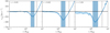Fig. 1. Galaxy radial velocity profiles, infalling shells, and turnaround radii. The solid blue curves show the average galaxy radial velocity profiles for redshifts z = 0.01, z = 0.62, and z = 1.04 (left, middle, and right panels, respectively). The dashed blue curves show the Savitzky-Golay smoothed profiles based on a ten-bin window (Savitzky & Golay 1964). The shadowed region shows the error in the smoothed profile. The vertical black line shows the average turnaround radius based on the velocity profiles. In each panel the blue vertical band indicates the infalling shell with boundaries at cluster-centric radii where the velocity is 0.72vmin (Sect. 4).

The curves show three clear regimes. Within $\sim 1R_{200\mathrm{c}}^{3\mathrm{D}}$, the average radial velocity has a plateau at zero or small velocity. This region is virialized because it has no net infall. At larger distances from the cluster center, $\sim (1-4)R_{200\mathrm{c}}^{3\mathrm{D}}$ (i.e., the infall region), the radial velocity is definitely non-zero and directed toward the cluster center. Finally, at distances ≳4R₂₀₀, the galaxy velocity is directed out of the cluster because the galaxies are still coupled to the universal Hubble flow.

Estimation of the MAR according to Eq. (3) requires determination of the minimum of the radial velocity profile (see Sects. 3 and 4). At each redshift, we measured the minimum velocity of the smoothed average radial profile. The first three columns of Table 3 list the minimum radial velocity, v_min, and its cluster-centric location, R_vmin, for each redshift bin. To compute the error in R_vmin, we bootstrapped 1000 samples of clusters at each redshift (Table 2, Cols. 1 and 2).

Table 2 shows that the median cluster mass generally decreases as the redshift increases because very massive systems are progressively less abundant at greater redshift. We checked the impact of the changing distribution of cluster masses on R_vmin. For each redshift, we built homogeneous samples that include only clusters with mass $M_{200\mathrm{c}}^{3\mathrm{D}}$ in the range (1.02 − 4.30)×10¹⁴ M_⊙. The largest minimum and smallest maximum mass for the samples in the 11 redshift bins set this range (see last column of Table 2). According to the Kolmogorov-Smirnov test, these clipped samples share indistinguishable mass distributions; the p-values are in the range (0.4 − 0.9). For each redshift, we computed the average radial velocity profile for the clipped sample and located R_vmin. The R_vmin radii for these samples are within ≲1.7% of the R_vmin radii of the full samples. They are also unbiased. Hence the R_vmin radii are insensitive to the difference among the distribution of cluster masses at different redshifts.

Figure 2 shows v_min as a function of its R_vmin, color coded by redshift. The minimum velocity and its cluster-centric radius are strongly correlated with redshift. From z = 0.01 to z = 1.04, the v_min of clusters with approximately equal mass (Table 2) increases by ∼100% in absolute value. The corresponding R_vmin decreases by ∼40%.

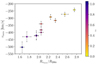Fig. 2. Minimum radial velocity as a function of the cluster-centric radius of the minimum (color coded by redshift).

The behavior of v_min as a function of redshift is in qualitative agreement with the general picture of hierarchical structure formation. For equal mass clusters, systems at higher redshift form within higher overdensity peaks. Because of their denser environment, these clusters are denser within ∼R_200c. Thus, more mass is confined within smaller cluster-centric radii than for an equally massive lower redshift cluster. The consequently deeper gravitational potential within ∼R_200c at greater redshift is the source of the larger minimum infall velocity located at smaller cluster-centric radius. The corresponding mass accretion is also larger in these higher redshift and denser environments. N-body simulations (e.g. van den Bosch 2002; McBride et al. 2009; Fakhouri et al. 2010; van den Bosch et al. 2014; Diemer et al. 2017) showed that, at fixed mass, the accretion rate at z ∼ 1 exceeds the rate at z ∼ 0 by roughly an order of magnitude.

The dynamics within the infall region is independent of the turnaround radius where galaxies depart from the Hubble flow as a result of the cluster potential (Gunn et al. 1972; Silk 1974; Schechter 1980). We identified the turnaround radius from the smoothed radial velocity profiles. Starting from the largest cluster-centric distances, the turnaround radius is the first intersection between the profile and the axis v_rad = 0. The vertical solid lines in Fig. 1 show that the turnaround radii agree well with Villumsen & Davis (1986). The turnaround radii are in the range (4.52 − 4.78)R_200c, ∼(2 − 3)R_200c beyond R_vmin. In contrast with R_vmin, the turnaround radius decreases by only ∼3.3% as the redshift increases from z = 0.01 to z = 1.04.

3. Recipe for the estimation of the mass accretion rate

The average radial velocity profiles (Sect. 2.2, Fig. 1) have clear minima at cluster-centric radii ∼(2 − 3)R_200c, identifying the region where clusters accrete new material. For an ideal, theoretical MAR (hereafter, MAR_t), we first calculated the rate at which material falls through an infinitesimal shell at this minimum velocity. However, real and simulated systems have too few galaxies in this shell. Thus, we derived a second MAR in a larger volume that approximates MAR_t. We analyzed the TNG300-1 run of IllustrisTNG to relate the observational MAR to MAR_t.

Assuming spherical symmetry, the mass of an infinitesimal shell at a distance r from the cluster center is dM_shell = 4πρ(r)r²dr, where dr is the width of the shell and ρ is the shell density. The time derivative of the shell mass is Ṁ = dM_shell/dt, where dt = dr/v_rad(r) is the time for infalling material with velocity v_rad(r) to cross dr. We defined MAR${}_t=\dot{M}(R_{v_{min}})$, where R_vmin is the minimum in the radial velocity profile (Sect. 2.2, Fig. 1, and Table 3):

$$\begin{array}{c}\hfill {\mathrm{MAR}}_t=4\pi \rho (R_{v_{min}})R_{v_{min}}^2{v}_{min}.\end{array}$$(2)

IllustrisTNG provides an estimate of MAR_t for a thin, finite shell where the radial velocity ≈v_min is nearly constant across the shell.

Observations can only provide the mass of an infalling shell with a finite width, ΔR ≫ dr. We defined the observational MAR of clusters of galaxies as the accretion of matter within a spherical shell onto the virialized region of the cluster:

$$\begin{array}{c}\hfill \text{MAR}=\frac{\text{d}M}{\text{d}t}=\mathcal{K}\frac{M_{\mathrm{shell}}}{t_{\inf }},\end{array}$$(3)

where M_shell is the mass of an infalling shell with width ΔR, t_inf is the time for the shell to accrete onto R_200c, and 𝒦 is a scaling factor. In an infinitesimal shell (ΔR = dr) located at R_vmin, the shell mass is $M_{\text{shell}}=4\pi \rho (R_{v_{\min }})R_{v_{\min }}^2\text{d}r$. If t_inf = dr/v_min and 𝒦 = 1, Eqs. (3) and (2) are equivalent. Below, we derive 𝒦 for thick shells of finite width.

Deriving the MAR from Eq. (3) depends on estimates of the mass in the infalling shell and the infall time. The caustic method provides the mass of the infalling shell from observations (Diaferio & Geller 1997; Diaferio 1999; Serra et al. 2011; Pizzardo et al. 2023). To calibrate this technique, we computed the true mass of the shell by summing the mass of dark matter, gas, stars, and black holes in a shell of width ΔR.

There is no direct observational route to the infall time because v_inf is currently inaccessible to observation. Although t_inf depends on redshift, it is fairly independent of cluster mass (see Fig. 7 below). Thus, the combination of M_shell from observations and t_inf derived from simulations yield an MAR based on cluster observations.

To compute the infall time, we solved the equation of radial infall with a nonconstant acceleration derived from the true gravitational potential of the cluster. The parameters of the equation are the initial infall velocity of the infalling shell, v_inf; the center of the infalling shell equivalent to the radial location of v_inf, R_vmin; and the radius that defines the virialized region of clusters, R_200c (Sect. 4.2).

We located the infalling shell (Sect. 4.1) from the simulated radial velocity profile of the cluster (Sect. 2.2). The boundaries of the infalling shell are R_shell, i (inner cluster-centric radius) and R_shell, o (outer cluster-centric radius), where the smoothed radial velocity is a fraction A of v_min.

To link MARs in Eq. (3) with MAR_t, we computed MARs with a range of A = 0.45–0.95. Smaller values of A overlap with the virialized regions of clusters, whereas larger values of A approach the ideal, theoretical limit in Eq. (2). However, MAR estimates for these thin shells are less robust because the number of simulated particles in the infalling shell is small.

We compared MAR^C and MAR^3D, the MARs estimated according to Eq. (3) respectively using $M_{\mathrm{shell}}^{\mathrm{C}}$ and $M_{\mathrm{shell}}^{3\mathrm{D}}$, the caustic and 3D shell masses, for 𝒦 = 1. Averaging over redshift, the median ratio between MAR^3D and MAR^C, r_3c, increases monotonically from r_3c = 0.92 ± 0.05 (A = 0.45) to r_3c = 1.09 ± 0.04 (A = 0.95). The error in r_3c is the interquartile range of the 11 ratios at the redshifts we considered. We adopted A = 0.72, where r_3c = 1.00 ± 0.04, as the best value. The choice of A = 0.72 provides a large enough galaxy sample for application of the caustic technique. The shaded blue vertical regions in Fig. 1 show shells with A = 0.72 for three redshifts: z = 0.01, z = 0.62, and z = 1.04 (left to right, respectively).

Finally, we connected MARs estimated in extended shells to MAR_t and estimated the appropriate value for 𝒦. Colored lines in Fig. 3 show the ratio MAR^3D(A)/MAR^3D(A = 0.72) as a function of A at six different redshifts, from z = 0.01 to z = 1.04, for 𝒦 = 1. The error bar shows the interquartile range of the ratios at A = 0.72. The estimated MARs decrease as A increases.

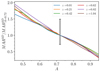Fig. 3. Relation between MAR and MARt. The curves show MAR3D(A)/MAR3D(A = 0.72) as a function of A in the range of 0.45 − 0.95 for six redshifts from z = 0.01 to z = 1.04. The error bar shows the median interquartile range of the ratio at A = 0.72.

When A = 0.95, the radial velocity is nearly constant across the shell and is (0.97–0.98)v_min. This thin shell provides an approximation of MAR_t. Averaging over the 11 redshifts, the ratio MAR^3D(A = 0.95)/MAR^3D(A = 0.72) is 𝒦 = 0.35. This value provides a plausible scaling between MAR_t and the M_shells and MARs estimated from cluster observations with A = 0.72.

4. Mass of the infalling shell and infall time from 3D and caustic mass profiles

Computation of the MAR of clusters requires an estimate of the mass of the infalling shell, M_shell, and of the infall time for the cluster to accrete the shell, t_inf. In Sect. 4.1, we describe the determination of M_shell. Section 4.2 presents the derivation of the infall time, t_inf.

4.1. The infalling shell and its mass

The average radial velocity profiles (Sect. 2.2; Fig. 1) are the basis for determining the cluster-centric radius of the infalling shell. The radial velocity profiles in Sect. 2.2 show a clear infall pattern at radii ∼(2 − 3)R_200c, where the minimum radial velocity occurs. Table 3 lists the average minimum radial velocity, v_min, and its radial location, R_vmin, at each redshift.

Based on the discussion in Sect. 3, we identified the inner (R_shell, i) and outer (R_shell, o) boundaries of the infalling shell where the smoothed radial velocity is 0.72v_min (A = 0.72; shaded blue vertical regions in Fig. 1). Table 3 (fifth column) shows the radial location of the infalling shell at each redshift. The cluster-centric distance of the shells decreases as redshift increases. At low redshifts, z ≲ 0.4, the shells are located in the range ∼(1.6 − 3.4)R_200c, whereas at high redshifts, z ≳ 0.73, the shells are in the range ∼(1.3 − 2.6)R_200c. This variation results from the decrease of R_vmin with increasing redshift (Sect. 2.2, see Fig. 2). The width of the infalling shell, ∼(1.2 − 1.3)R_200c, is nearly redshift independent.

For each simulated cluster, we computed the true mass, $M_{\mathrm{shell}}^{3\mathrm{D}}(A=0.72)$, and caustic observable mass, $M_{\mathrm{shell}}^{\mathrm{C}}(A=0.72)$, of the infalling shell. For the appropriate radial range (Table 3), we computed two true and caustic masses that measure M(< R_shell, i; A = 0.72), the total mass within the inner boundary of the shell, and M(< R_shell, o; A = 0.72), the total mass within the outer boundary of the shell. The observable mass of the infalling shell is thus the difference between these masses: M_shell(A = 0.72) = M(< R_shell, o; A = 0.72)−M(< R_shell, i; A = 0.72).

Figure 4 shows the true $M_{\mathrm{shell}}^{3\mathrm{D}}=\mathcal{K}{M}_{\mathrm{shell}}^{3\mathrm{D}}(A=0.72)$ as a function of the true $M_{200\mathrm{c}}^{3\mathrm{D}}$ at three different redshifts: z = 0.01, z = 0.62, and z = 1.04 (cyan, violet, and magenta, respectively). The squares with error bars show the medians and interquartile ranges of the simulated data in eight logarithmic mass bins covering the range (1 − 12.6)  ×  10¹⁴ M_⊙. The lines show a power law fit to the data.

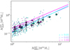Fig. 4. Relation between $M_{\mathrm{shell}}^{3\mathrm{D}}$ and $M_{200\mathrm{c}}^{3\mathrm{D}}$. The colored circles show $M_{\mathrm{shell}}^{3\mathrm{D}}$ as a function of $M_{200\mathrm{c}}^{3\mathrm{D}}$ in the three redshift bins z = 0.01, 0.62, and 1.04 (cyan, violet, and magenta, respectively). The squares with error bars indicate the median and interquartile range in eight fixed logarithmic mass bins. The lines show power law fits to the data.

At every redshift, $M_{\mathrm{shell}}^{3\mathrm{D}}$ and $M_{200\mathrm{c}}^{3\mathrm{D}}$ are strongly correlated: a change of one order of magnitude in mass leads to a comparable change in the mass of the infalling shell. Kendall’s test provided a correlation index of ∼0.44, with associated p-values in the range ∼10⁻⁵ − 10⁻²⁸. This correlation is expected in the hierarchical cluster formation model because, at fixed redshift, higher mass clusters reside within greater overdensities, and thus there is more mass in their accreting shells. Conversely, M_shell is not strongly correlated with redshift. Although the fits show that $M_{\mathrm{shell}}^{3\mathrm{D}}$ generally increases by ∼20 − 60% from z = 0.01 to z = 1.04, the error bars show that this correlation is not statistically significant.

The colored points in Fig. 5 show $M_{\mathrm{shell}}^{3\mathrm{D}}$ as a function of redshift for individual clusters in 11 redshift bins. The data are coded by cluster mass $M_{200\mathrm{c}}^{3\mathrm{D}}$. The 11 transparent black circles with error bars indicate the median and interquartile range of $M_{\mathrm{shell}}^{3\mathrm{D}}$ in each redshift bin.

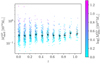Fig. 5. Relation between $M_{\mathrm{shell}}^{3\mathrm{D}}$ and redshift. The small circles show the $M_{\mathrm{shell}}^{3\mathrm{D}}$ of individual clusters as a function of redshift, color coded by $M_{200\mathrm{c}}^{3\mathrm{D}}$. The points include clusters over the entire redshift range. We introduced an artificial jitter on the exact redshifts to make the dependence of $M_{\mathrm{shell}}^{3\mathrm{D}}$ on $M_{200\mathrm{c}}^{3\mathrm{D}}$ more evident. The transparent black circles with error bars show the median and interquartile range of $M_{\mathrm{shell}}^{3\mathrm{D}}$ in each redshift bin.

Figure 5 shows the same trend observed in Fig. 4 between $M_{\mathrm{shell}}^{3\mathrm{D}}$ and $M_{200\mathrm{c}}^{3\mathrm{D}}$. At fixed redshift, $M_{\mathrm{shell}}^{3\mathrm{D}}$ increases with $M_{200\mathrm{c}}^{3\mathrm{D}}$: a change of approximately one order of magnitude in $M_{200\mathrm{c}}^{3\mathrm{D}}$ corresponds to an analogous change in $M_{\mathrm{shell}}^{3\mathrm{D}}$. The median $M_{\mathrm{shell}}^{3\mathrm{D}}$s, denoted by the transparent black circles in the figure, are uncorrelated with redshift.

The dependence of M_shell and redshift is expected in the standard model of structure formation and evolution. In Appendix A, we explain how a complex interplay between the density and mass profiles as a function of redshift along with the slightly different cluster mass distribution at various redshifts tends to suppress any correlation between M_shell and redshift.

The caustic technique provides robust estimates of the mass profile of clusters in the infalling shell (Pizzardo et al. 2023). Points with error bars in Fig. 6 show the median and the interquartile range of individual ratios between the caustic and true mass $M_{\mathrm{shell}}^{\mathrm{C}}/M_{\mathrm{shell}}^{3\mathrm{D}}$ as a function of redshift. Analogously to $M_{\mathrm{shell}}^{3\mathrm{D}}$, we defined $M_{\mathrm{shell}}^{\mathrm{C}}=\mathcal{K}{M}_{\mathrm{shell}}^{\mathrm{C}}(A=0.72)$. Because the infalling region is closer to the cluster center as the redshift increases (Table 3, fifth column), the median ratio slowly rises from 0.9 at z = 0 to 1.1 at z = 1.04¹. The typical dispersion in the ratio is ∼34%. Thus, the caustic technique slightly overestimates or underestimates the mass at smaller and larger cluster-centric distances, respectively. The trend is not statistically significant, as Kendall’s τ correlation coefficient is ≲0.05. The caustic mass $M_{\mathrm{shell}}^{\mathrm{C}}$ is an unbiased estimate of $M_{\mathrm{shell}}^{3\mathrm{D}}$. Furthermore, $M_{\mathrm{shell}}^{\mathrm{C}}$ has the same dependence on mass, redshift, and R_vmin as $M_{\mathrm{shell}}^{3\mathrm{D}}$, on average.

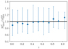Fig. 6. Median and interquartile ranges of the ratio between the caustic and true Mshell as a function of redshift.

4.2. The infall time

Based on the full 3D cluster properties at each redshift, we computed t_inf, the time for an infalling shell to accrete onto the virialized region of the cluster. We derived t_inf by tracking the radial infall with nonconstant acceleration driven by the cluster gravitational potential. The locations of the minima in the average radial velocity profiles (Sect. 2.2) set the limit of the radial range where we computed the infall time. We ultimately employed the infall times based only on the true full 3D data because the uncertainty in these measures derived by application of the caustic method is too large.

We computed the time for the center of the infalling shell to reach R_200c as a measure of t_inf. We measured the infall time starting from the radius of the minimum infall velocity, R_vmin (Fig. 1 and Table 3). In other words, t_inf is the time required for the center of the infalling shell initially located at R_vmin to reach R_200c.

Over the radial range R_vmin to R_200c, the gravitational acceleration changes substantially. To compute the t_inf of each cluster in each redshift bin, we used an iterative procedure. We divided the radial range (R_200c, R_vmin) into N + 1 = 101 bins. The radial step between two contiguous bins is Δr = (R_vmin − R_200c)/N. The N + 1 steps n = 0, 1, …, N correspond to r₀ = R_vmin, r₁ = R_vmin − Δr, …, r_N = R_200c. At each step n < N, we calculated Δt_n, the time for the center of the shell to move from r_n = R_vmin − nΔr to r_n + 1 = R_vmin − (n + 1)Δr. Within this small radial interval with Δr ∼ 0.01R_200c ≈ 0.01 Mpc, the gravitational acceleration is nearly constant. From this acceleration and the initial infall velocity of the shell, a_n and v_n, respectively, we computed Δt_n as the positive (physical) solution of the equation

$$\begin{array}{c}\hfill \frac{a_n}{2}\mathrm{\Delta }{t}_n^2+v_n\mathrm{\Delta }{t}_n+\mathrm{\Delta }r=0,\end{array}$$(4)

that is²,

$$\begin{array}{c}\hfill \mathrm{\Delta }{t}_n=\frac{-v_n-\sqrt{v_n^2-2a_n\mathrm{\Delta }r}}{a_n}.\end{array}$$(5)

We obtained the acceleration of the infalling shell by computing the cluster gravitational potential ϕ(r) based on the true cluster shell density profile ρ(r). The Poisson equation for an isolated spherical system with shell density profile ρ_I(r) is

$$\begin{array}{c}\hfill \varphi (r)=-4\pi G[\frac{1}{r}{\displaystyle {\int }_0^r}{\rho }_I(r)r^2\text{d}r+{\int }_r^{+\infty }{\rho }_I(r)r\text{d}r].\end{array}$$(6)

The uniform cosmological background density, ⟨ρ(z)⟩ = Ω_M(z)ρ_c(z), exerts no net gravitational effect. Thus, we computed the gravitational potential based on the mass density fluctuations by replacing ρ_I(r) with ρ(r)−⟨ρ⟩. The second integral is finite; at sufficiently large cluster-centric distances, ∼10R_200c (see Appendix A), the correlated cluster density is ∼0. We replaced the upper limit of the second integral of Eq. (6) with 10R_200c.

From the true cluster potential ϕ(r), we computed the gravitational acceleration induced by the cluster, a(r), by simple differentiation: $a(r)=-\frac{\text{d}}{\text{d}r}\varphi (r)$. At each step n, we set a_n (Eq. (4)) to the value of a(r) at the position of the center of the infalling shell, a_n = a(R_vmin − nΔr).

At the first step n = 0, the initial velocity is v₀ = v_inf, where v_inf is the average cluster radial velocity of the infalling shell at that redshift (fourth column of Table 3). At each succeeding step n, we incrementally increased the initial infall velocity of the shell by taking a constant acceleration in the small time step: v_n = v_n − 1 + a_n − 1Δt_n − 1.

The application of Eq. (5) from n = 0 to n = N − 1 yielded a set of N time steps, Δt_{n = {0, …, N − 1}}. The sum of these time steps is our estimate of the cluster infall time:

$$\begin{array}{c}\hfill t_{\inf }={\displaystyle \sum _{n=0}^{N-1}}\mathrm{\Delta }{t}_n.\end{array}$$(7)

Figure 7 shows the resulting infall times for individual clusters as a function of $M_{200\mathrm{c}}^{3\mathrm{D}}$ in three redshift bins: z = 0.01, 0.62, and 1.04 (cyan, violet, and magenta, respectively). The squares with error bars show the medians and interquartile ranges of the simulated data in eight logarithmic mass bins covering the range (1 − 12.6)×10¹⁴ M_⊙ (as in Fig. 4). The lines show a power law fit.

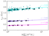Fig. 7. Relation between tinf and $M_{200\mathrm{c}}^{3\mathrm{D}}$. The colored circles show tinf of individual clusters as a function of their mass $M_{200\mathrm{c}}^{3\mathrm{D}}$ in the three redshift bins z = 0.01, 0.62, and 1.04 (cyan, violet, and magenta, respectively). The squares with error bars indicate the median and the interquartile range in eight fixed logarithmic bins of mass. The lines show power law fits to the data.

The infall time t_inf is correlated with redshift. The increased cluster radial acceleration resulting from the larger cluster density at high redshift produces this correlation (Eq. (6)). Equation (5) shows that the increased acceleration produces a corresponding decrease in the infall time t_inf.

The squares in Fig. 7 show the absence of correlation between t_inf and the cluster mass $M_{200\mathrm{c}}^{3\mathrm{D}}$ at each redshift. The higher density of more massive clusters generates a larger acceleration decreasing t_inf. However, more massive clusters are also more extended, thus increasing the radial range (R_200c, R_vmin) and correspondingly increasing t_inf. These effects result in a minimal dependence of t_inf on $M_{200\mathrm{c}}^{3\mathrm{D}}$.

5. The mass accretion rate

We applied Eq. (3) to estimate the MARs at different redshifts. We computed MAR^3D, the true MAR based on $M_{\mathrm{shell}}^{3\mathrm{D}}$ and t_inf, and MAR^C, the caustic MAR based on $M_{\mathrm{shell}}^{\mathrm{C}}$. As described earlier, we used 3D data to model the infall time. We compared MAR^C with MAR^3D to assess the caustic technique as a robust method for estimating the true MAR.

According to Eq. (3), the MAR^3D of each individual cluster is the ratio between its respective $M_{\mathrm{shell}}^{3\mathrm{D}}$ (see Sect. 4.1) and t_inf (see Sect. 4.2). Figure 8 shows the true MARs of individual clusters as a function of $M_{200\mathrm{c}}^{3\mathrm{D}}$ in three different redshift bins: z = 0.01, 0.62, and 1.04 (cyan, violet, and magenta, respectively). The squares with error bars show the medians and interquartile ranges of the simulated data in eight logarithmic mass bins covering the range (1 − 12.6)  ×  10¹⁴ M_⊙. The lines show a power law fit.

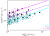Fig. 8. Relation between MAR3D and $M_{200\mathrm{c}}^{3\mathrm{D}}$. The colored circles show MAR3D as a function of $M_{200\mathrm{c}}^{3\mathrm{D}}$ in the three redshift bins z = 0.01, 0.62, and 1.04 (cyan, violet, and magenta, respectively). The squares with error bars show the median and interquartile range in eight fixed mass bins. The lines show power law fits to the data.

The MARs increase both with increasing mass and with increasing redshift. A correlation between MAR and M_200c is expected because more massive clusters tend to be surrounded by larger amounts of mass. Figure 8 shows that at fixed redshift, a change of approximately one order of magnitude in $M_{200\mathrm{c}}^{3\mathrm{D}}$ corresponds to an analogous change in MAR^3D. This correlation with mass follows from the correlation between M_shell and M_200c (Sect. 4.1). Figures 8 and 4 show that the increase of MAR^3D with $M_{200\mathrm{c}}^{3\mathrm{D}}$ is consistent with the increase of $M_{\mathrm{shell}}^{3\mathrm{D}}$ with $M_{200\mathrm{c}}^{3\mathrm{D}}$. Figure 7 shows that the infall time does not play a significant role in this correlation.

In the hierarchical clustering paradigm, clusters of fixed mass at higher redshift reside within denser regions and thus accrete faster than clusters of the same mass at lower redshift. Figure 8 shows that at fixed mass, MAR^3D increases by a factor of ∼2.2 from z = 0.01 to z = 0.62, and by a factor ∼5 from z = 0.01 to z = 1.04. This effect originates from the anticorrelation between t_inf and the redshift (Sect. 4.2). Figures 8 and 7 show that the increase of MAR^3D with increasing redshift is consistent with the decrease of t_inf with increasing redshift.

We fit the individual MAR^3Ds and $M_{200\mathrm{c}}^{3\mathrm{D}}$s at each redshift to the relation MAR$=a{(M_{200\mathrm{c}}^{3\mathrm{D}}/{10}^{14}{M}_{\odot })}^b$ (Table 4). The fits show the expected tight correlation between MAR and redshift. The coefficient a that measures the MAR at fixed mass increases with redshift by a factor approximately seven from z = 0.01 to z = 1.04. The slope of the power law is essentially redshift independent. The average of the 11 slopes b’s yields a mean slope of $\overline{b}=0.90\pm 0.18$ in the redshift range 0.01 − 1.04.

We fit the analytic relation proposed by Fakhouri et al. (2010) to the MAR as a function of redshift:

$$\begin{array}{c}\hfill {\text{MAR}}^{3\mathrm{D}}=U[M_{\odot }{\text{yr}}^{-1}]{\left(\frac{M_{200\mathrm{c}}^{3\mathrm{D}}}{{10}^{12}{M}_{\odot }}\right)}^V(1+Wz)\sqrt{{\mathrm{\Omega }}_{\mathrm{m}0}{(1+z)}^3+{\mathrm{\Omega }}_{\mathrm{\Lambda }0}}.\end{array}$$(8)

Because of the limited mass range we sampled at greater redshifts, we fixed $V=\overline{b}$ and we fit the median MAR^3D as a function of the median $M_{200\mathrm{c}}^{3\mathrm{D}}$ and the redshift. The resulting coefficients are: U = 128 ± 13, $V=\overline{b}=0.90\pm 0.18$, and W = 1.69 ± 0.34. We compare these results with earlier work in Sect. 6.

The MAR^C of individual clusters is the ratio between $M_{\mathrm{shell}}^{\mathrm{C}}$ and the infall time $t_{\inf }^{\mathrm{fit}}(M_{200\mathrm{c}}^{\mathrm{C}})$ (Sect. 4.2), where we based the computation on the cluster caustic mass $M_{200\mathrm{c}}^{\mathrm{C}}$. We computed the cluster infall time $t_{\inf }^{\mathrm{fit}}(M_{200\mathrm{c}}^{\mathrm{C}})$ by evaluating the power law fit of the individual infall times at the cluster caustic mass $M_{200\mathrm{c}}^{\mathrm{C}}$ as a function of mass derived by true profiles at the given redshift (Fig. 7). The upper panel of Fig. 9 shows the median and interquartile range of the true (blue squares and solid error bars) and caustic (red triangles and dotted error bars) MARs as a function of redshift. The black curve is a fit of Eq. (8) to the MARs as a function of redshift. We fixed the mass to the median mass of the cluster sample. The residuals around the fit are, on average, only ∼ − 0.6%. The black dots in the lower panel show the ratios between the median values of the caustic and true MARs.

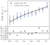Fig. 9. Comparison between MARC and MAR3D. Upper panel: median true (blue squares) and caustic (red triangles) MARs as a function of redshift. The solid blue and dotted red error bars show the interquartile ranges of the true and caustic MARs, respectively. The black curve shows a fit to Eq. (8). Lower panel: median ratio (black dots) between the caustic and true MARs as a function of redshift.

The figure shows that MAR^C is a robust platform for estimating the true MAR^3D at every redshift. The median MAR^Cs are within 15% of the median MAR^3Ds at each redshift. The caustic MARs are also unbiased relative to the true MARs. Thus, the caustic technique provides accurate and robust estimates of the MARs of clusters in the redshift range 0.01 − 1.04.

6. Discussion

We used the TNG300-1 run of the IllustrisTNG simulations to estimate the MAR of galaxy clusters based on the radial velocity profile of cluster galaxies and on the cluster total mass profile. The caustic technique provides robust and unbiased estimates of the true MARs derived from 3D data over the redshift range 0.01 − 1.04.

In the following subsection (Sect. 6.1), we compare the IllustrisTNG results with previous work on simulated and observed clusters. In Sect. 6.2, we assess the bias between the galaxy MARs and MARs derived from the dark matter halos for the same sample of clusters drawn from the IllustrisTNG simulations. In Sect. 6.3, we discuss future simulations and observational applications of the MAR.

6.1. Comparison with previous results

The dynamically motivated MAR recipe we developed differs significantly from previous merger tree approaches (e.g., McBride et al. 2009; Fakhouri et al. 2010; van den Bosch et al. 2014; Correa et al. 2015b; Diemer et al. 2017; Diemer 2018). In contrast with a merger tree procedure that is not directly observable, the approach we outline allows the estimation of the MAR of real clusters and comparison with the true MARs of comparable simulated systems.

Most previous theoretical investigations of the MAR are based on N-body dark matter only simulations. These studies employ merger trees that trace the mass accretion of a halo at z = 0 back in time. The merger trees follow the change in mass between the halo descendant on the main branch identified at z_i > 0 and its most massive progenitor for z_i + Δz, where Δz is the time step. The details of the simulation, including the halo fragmentation algorithm and the choice of mass and time step, may affect the results (Diemer 2018; Xhakaj et al. 2019). Some studies (e.g., van den Bosch et al. 2014; Correa et al. 2015a,b) are based on the analytic or semi-analytic extended Press-Schechter formalism (Bond et al. 1991) calibrated with N-body simulations.

The upper panel of Fig. 10 compares MARs from Fig. 8 (squares) with two merger tree calculations based on N-body simulations by Fakhouri et al. (2010, Eq. (2)³; dotted lines), and Diemer et al. (2017, Eqs. (9) and (10); solid lines).

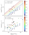Fig. 10. Comparison between our MARs and previously published results. Upper panel: squares show MAR3Ds from Fig. 8 as a function of $M_{200\mathrm{c}}^{3\mathrm{D}}$ and color coded by redshift, from dark blue to dark red as the redshift increases from bin to bin: z = 0.01, 0.21, 0.52, 0.82, and z = 1.04. The lines show MARs from merger trees by Fakhouri et al. (2010, dotted line) and by Diemer et al. (2017, solid line). Lower panel: squares again show the true MARs from TNG300-1 as a function of $M_{200\mathrm{c}}^{3\mathrm{D}}$. Triangles show the MAR3Ds from Pizzardo et al. (2022) as a function of $M_{200\mathrm{c}}^{3\mathrm{D}}$ in four redshift bins: z = 0.01, 0.19, 0.44, and z = 1.00. The stars show the MARs of ten observed stacked clusters from the HectoMAP survey (Pizzardo et al. 2022).

Fakhouri et al. (2010) extended the McBride et al. (2009) investigation of the Millennium simulation (Springel et al. 2005) to Millennium II (Boylan-Kolchin et al. 2009). For the mass of each FoF halo, they took the sum of the masses of their subhalos. They then computed the MARs from one snapshot to the next. The results by Fakhouri et al. (2010) are in excellent agreement with the earlier results by McBride et al. (2009) and the later results by van den Bosch et al. (2014, see their Fig. 12 and by Correa et al. 2015a,b).

Diemer et al. (2017) used a large set of ΛCDM N-body simulations run with GADGET2 (Springel et al. 2005). They used M_200m as a halo mass proxy and computed the MARs at time steps comparable with the halo dynamical time (Diemer 2017)⁴.

The merger tree MARs depend on the subhalo finder, the merger tree builder, and the definition of MAR. The difference between the two merger tree models in the upper panel of Fig. 10 shows the impact of these underlying differences. At each time step a merger tree MAR generally results from the difference between the mass of the descendant and the mass of the most massive progenitor. The most massive progenitor may not be the main branch progenitor (see Fakhouri et al. 2010, for more details), and thus the MAR is a lower limit. The halo mass definition may also vary. In the Fakhouri et al. (2010) model, the mass is the sum of the masses of the subhalos. In Diemer et al. (2017), the mass definition is M_200m, which is the mass enclosed within a sphere centered on the halo center with matter density equal to 200 times the background matter density. The choice of time step can also affect the MARs (Xhakaj et al. 2019). In Sect. 6.2, we demonstrate that the use of dark matter only simulations may also bias the MARs toward lower values, but the bias is small.

Figure 11 compares the fits to the IllustrisTNG MARs using Eq. (8) (see Sect. 5; solid line) with Fakhouri et al. (2010; dotted line) and Diemer et al. (2017; dashed line) at z = 0.31. In all models, the MAR increases with cluster mass. Because Fakhouri et al. (2010) and Diemer et al. (2017) do not report errors in their fits, we assumed fractional errors comparable with ours (shadowed areas). The slope of the IllustrisTNG MAR thus agrees with Fakhouri et al. (2010) and Diemer & Kravtsov (2014). When averaged over the entire redshift range, the slope of the IllustrisTNG MARs as a function of $M_{200\mathrm{c}}^{3\mathrm{D}}$ is 0.90 ± 0.18 (Sect. 5), which is in agreement with the slopes of 1.1–1.2 obtained by Fakhouri et al. (2010) and Diemer et al. (2017).

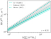Fig. 11. Comparison between fits to our MARs and previously published fits. The solid, dotted, and dashed lines show the fit of the analytic relation proposed by Fakhouri et al. (2010) to the IllustrisTNG MARs (Eq. (8), see Sect. 5), the fit by Fakhouri et al. (2010), and the fit by Diemer et al. (2017), respectively, at z = 0.31. The shadowed turquoise band shows the typical 1σ IllustrisTNG scatter. The gray shadow indicates a similar assumed scatter for the merger tree models (gray bands).

The IllustrisTNG MARs are consistent with merger tree MARs at every redshift (upper panel of Fig. 10). Assuming similar fractional errors for Fakhouri et al. (2010) and Diemer et al. (2017) and IllustrisTNG, the 0–50% difference in the rates is usually within the 1σ error and always within the 2σ error. The shaded regions in Fig. 11 indicate the general consistency of the results. The difference between the IllustrisTNG and merger tree MARs increases as the redshift increases, but so does the error (Table 4). The parameter W of Eq. (8) characterizes the redshift dependence of the MAR. The IllustrisTNG simulations yield W = 1.69 ± 0.34 (Sect. 5). Notably, Fakhouri et al. (2010) obtained W = 1.17. The difference is ≲2σ. The qualitative agreement between the IllustrisTNG and merger tree approaches is reassuring given the substantial differences in the algorithms.

Based on the spherical accretion prescription proposed by De Boni et al. (2016), Pizzardo et al. (2021) developed the first systematic approach to estimating the MARs of real clusters. Pizzardo et al. (2021) computed the MAR as the ratio between the mass of an infalling shell and the infall time. Their approach is similar to the IllustrisTNG approach we follow, but they used a ΛCDM N-body dark matter only simulation.

Pizzardo et al. (2022) applied the Pizzardo et al. (2021) recipe to ten stacked clusters from the HectoMAP redshift survey (Sohn et al. 2021b,a). They also derived MARs based on the ΛCDM N-body simulation L-CoDECS (Baldi 2012). The bottom panel of Fig. 10 shows the simulated MARs (triangles) and the observed MARs of HectoMAP stacked clusters (stars) as a function of mass and color coded by redshift compared with TNG300-1 (squares).

The HectoMAP MARs are consistent with the TNG300-1 MARs. The agreement between MARs of observed clusters and TNG300-1 may reflect the use of simulated galaxies to calibrate the MAR derived from IllustrisTNG.

6.2. The dark matter mass accretion rate

Previous theoretical work on the MAR is based on N-body dark matter only simulations. Galaxies are generally biased tracers of the underlying distribution of dark matter (e.g., Kaiser 1984; Davis et al. 1985; White et al. 1987). With TNG300-1, we can measure the bias by estimating the MAR for both galaxies and dark matter for the identical sample of clusters. We used 3D data from the simulation for this test.

We began by locating the infalling shell based on the dark matter. We followed the procedure outlined in Sect. 2.2, using the average radial velocity profiles of the dark matter particles. For each redshift bin, we computed the dark matter radial velocity profile of the individual clusters in 200 logarithmically spaced bins covering the radial range $(0-10)R_{200\mathrm{c}}^{3\mathrm{D}}$. We chose narrower binning for the dark matter profiles than we did for the galaxies because the number of dark matter particles is much larger than the number of galaxies.

We computed a single mean radial velocity profile and smoothed it as we did in Sect. 2.2. We identified the minimum radial velocity of the average profile, $v_{min}^{\mathrm{dm}}$, and its cluster-centric location, $R_{v_{min}}^{\mathrm{dm}}$. As in Sect. 2.2, the boundaries of the infalling are the cluster-centric distances where the average velocity is $0.72v_{min}^{\mathrm{dm}}$.

The average radial velocity profiles of dark matter and galaxies agree at every redshift. The radial location of $v_{min}^{\mathrm{dm}}$, $R_{v_{min}}^{\mathrm{dm}}$, is on average ∼0.04% (∼7.9% at most) smaller than R_vmin, based on the galaxies. The infall velocity based on the dark matter, $v_{\inf }^{\mathrm{dm}}$, is on average ∼2.1% (∼5.9% at most) less than v_inf, determined from the galaxies.

We computed the mass of the infalling shell, $M_{\mathrm{shell}}^{3\mathrm{D},\mathrm{dm}}$, and the shell infall time, $t_{\inf }^{\mathrm{dm}}$, from the dark matter field following Sects. 4.1 and 4.2 but based only on the mass profile of the dark matter component. To compute $M_{\mathrm{shell}}^{3\mathrm{D},\mathrm{dm}}$ and $t_{\inf }^{\mathrm{dm}}$, we multiplied the dark matter profile by (1 + Ω_b0/Ω_m0) to account for the baryonic fraction. The resulting MAR^3D, dm were then directly comparable with the MAR^3D computed based on the total mass profile.

Figure 12 shows a comparison of the dark matter and galaxy MARs. The blue squares and orange points in the upper panel show the median true MARs derived from galaxies and dark matter, respectively. The corresponding colored error bars show the interquartile ranges of the MARs. The black dots in the lower panel show the median ratio between the 3D MARs computed from dark matter and the 3D MARs from galaxies. The dash-dotted line shows the global median.

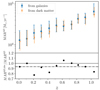Fig. 12. Comparison between MARs from galaxies and dark matter. Upper panel: blue squares (orange dots) and blue (orange) error bars show the median and the interquartile range of the true MARs based on galaxies (dark matter) as a function of redshift. Lower panel: points show the median ratio between the dark matter and galaxy MARs as a function of redshift. The dash-dotted line shows the median ratio.

On average, the dark matter MAR^3D, dms are ∼6.5% below the MARs based on the galaxies. The scatter between the two MARs is < 30%, generally less than the uncertainty in the determination of the respective MARs. Thus, the galaxies are indeed biased tracers, but the bias is small at these scales.

The MAR derived from galaxies should exceed the dark matter MAR because the clustering amplitude of galaxies relative to dark matter is larger at smaller scales and at higher redshift (Davis & Peebles 1983; Davis et al. 1985; Jenkins et al. 1998). On the scale of the accretion region of galaxy clusters with redshift z ≲ 1, the galaxy clustering excess is, however, small (Springel et al. 2018). Thus, the bias between the galaxy and dark matter MARs derived from IllustrisTNG is also small.

6.3. Future prospects

MARs of large samples of real and simulated clusters render the MAR a probe of cluster astrophysics (e.g., Vitvitska et al. 2002; Gao et al. 2004; van den Bosch et al. 2005; Kasun & Evrard 2005; Allgood et al. 2006; Bett et al. 2007; Ragone-Figueroa et al. 2010; Ludlow et al. 2013; Diemer & Kravtsov 2014; More et al. 2015; De Boni et al. 2016; Diemer et al. 2017) and cosmology (e.g., Diaferio 2004; Mantz et al. 2008, 2014, 2015; Walker et al. 2019; Cataneo & Rapetti 2020). The caustic technique (Diaferio & Geller 1997; Diaferio 1999; Serra et al. 2011) provides unbiased estimation of the true MAR in the wide redshift range 0.01 − 1.04. Measurement of the MAR of real clusters is currently limited to z ≲ 0.4 (Pizzardo et al. 2021, 2022).

Next generation wide-field spectroscopic surveys will observe the infall regions around large numbers of galaxy clusters with high sampling rates. These dense and deep spectroscopic surveys will provide the necessary observational baseline for measuring the MARs of thousands of clusters extending to higher redshifts.

The multi-object William Herschel Telescope Enhanced Area Velocity Explorer (WEAVE) spectrograph on the William Herschel Telescope (WHT; Balcells et al. 2010; Dalton et al. 2012, 2014; Dalton 2016) will explore the infall regions of galaxy clusters and their connections to the cosmic web. The WEAVE Wide-Field Cluster Survey (Cornwell et al. 2022, 2023) will measure thousands of galaxy spectra in and around 20 clusters with 0.04 < z < 0.07 out to radii ≲5R_200c. A deeper cluster survey will provide dense spectroscopic surveys of 100 clusters for redshift ≲0.5, a new baseline for measuring the MAR in this redshift range. Planned observations with the Prime Focus Spectrograph on Subaru (PFS; Tamura et al. 2016) and the Maunakea Spectroscopic Explorer on CFHT (MSE; Marshall et al. 2019) will provide spectroscopic redshifts of hundreds to thousands of galaxy cluster members for thousands of individual clusters with z ≲ 0.6.

The caustic technique (Diaferio & Geller 1997; Diaferio 1999) and weak gravitational lensing (Bartelmann 2010; Hoekstra et al. 2013; Umetsu 2020) will provide two independent measurements of cluster mass profiles extending to large radii. Neither the caustic technique nor weak lensing relies on the assumption of dynamical equilibrium. These techniques can thus be applied throughout the accretion region where dynamical equilibrium does not hold (Ludlow 2009; Bakels et al. 2021). Present weak-lensing maps from HST and Subaru already provide cluster mass profiles up to 5.7 Mpc for ∼20 systems (Umetsu et al. 2011, 2016). Future facilities will extend these measurements to thousands of clusters. The VRO (Ivezić et al. 2019) and the Euclid mission (Laureijs et al. 2011; Sartoris et al. 2016) will provide extended weak-lensing mass profiles for combination with extensive spectroscopy samples of clusters with z ≲ 2.

The TNG300-1 MARs are based on less than100 clusters at z > 0.52. The mass distribution of TNG300-1 mostly samples clusters with $M_{200\mathrm{c}}^{3\mathrm{D}}\sim (1.2-2)\times {10}^{14}$ M_⊙. High redshift massive clusters have larger MARs and place tight constraints on models of structure formation and evolution (e.g., Bardeen et al. 1986; White 2002). Larger volume hydrodynamical simulations, including MillenniumTNG (Pakmor et al. 2023), with its 740 Mpc comoving size, will provide larger samples of the most massive systems up to higher redshift. The next generation of simulations should enable tracing of the MAR to redshifts ≳1. Extension of MAR determination to early epochs in cluster history will provide new insights into the astrophysics of cluster formation and evolution.

7. Conclusion

We used the TNG300-1 run of the IllustrisTNG simulations (Pillepich et al. 2018; Springel et al. 2018; Nelson et al. 2019) to compute the MAR of clusters of galaxies. The recipe, based on the dynamics of cluster galaxies, computes the MAR as the ratio between the mass inside a spherical shell within the cluster infall region and the time for the shell to reach the virialized region of the cluster. The method builds on the approach by De Boni et al. (2016) and Pizzardo et al. (2021) and incorporates the caustic technique (Diaferio & Geller 1997; Diaferio 1999; Serra et al. 2011), which provides robust, unbiased estimates of the true MARs. Notably, IllustrisTNG refines the estimation of clusters’ MARs. It permits the derivation of true MARs in a narrow shell, an approach that provides improved scaling between observational and true MARs. A major goal of our approach is the direct application to cluster observations.

We used 1318 clusters extracted from TNG300-1 (Pizzardo et al. 2023). This sample includes both the 3D and caustic mass profiles of each cluster. The clusters have a median mass of $M_{200\mathrm{c}}^{3\mathrm{D}}\sim (1.3-1.6)\times {10}^{14}$ M_⊙ and cover the redshift range of 0.01 − 1.04. We located the infalling shell based on the average radial motion of cluster galaxies as a function of cluster-centric distance and redshift. We computed the infall time by solving the equation for radial infall of the infalling shell to R_200c with nonconstant acceleration derived from the true cluster gravitational potential.

The MARs increase with increasing cluster mass and redshift. At fixed redshift, a change of approximately one order of magnitude in M_200c yields a comparable increase in the MAR. This dependence tracks the increase of the mass of the infalling shell as a function of M_200c. At fixed mass, the MAR increases by a factor of approximately five, from z = 0.01 to z = 1.04, because of the anticorrelation of the infall time with redshift. The correlations between the MAR and cluster mass and redshift are predicted by hierarchical structure formation scenarios.

The MARs from IllustrisTNG build on similar approaches based on N-body simulations (e.g., Pizzardo et al. 2021, 2022). In TNG300-1, we can test the dark matter MARs against the galaxy MARs for the identical set of simulated systems. The dark matter MARs are ∼6.5% lower than the galaxy MARs, reflecting the relative amplitudes of the clustering of galaxies and dark matter as a function of scale and redshift.

The IllustrisTNG MARs complement approaches based on merger trees, which cannot be linked as directly to the observations (e.g., McBride et al. 2009; Fakhouri et al. 2010; Correa et al. 2015b; van den Bosch et al. 2014; Diemer et al. 2017; Diemer 2018). The IllustrisTNG MARs lie within 2σ of the merger tree results. On average, the IllustrisTNG MARs differs from the merger tree MARs by ∼0 − 50%; the difference increases with redshift. At fixed redshift, the dependence of the merger tree and IllustrisTNG MARs on cluster mass agree well. The IllustrisTNG MARs are remarkably consistent with available observations of the MAR as a function of redshift (Pizzardo et al. 2022).

Our approach using IllustrisTNG enables the exploration of accretion by galaxy clusters with simulated galaxies. The approach provides a framework for obtaining robust MARs based on observed spectroscopic samples with ≳200 cluster members. Future spectroscopic (e.g., with instruments like WEAVE, PFS, and MSE) and weak-lensing (e.g., with facilities like Euclid and VRO) surveys will provide such samples. The next generation of large volume hydrodynamical simulations including MillenniumTNG will guide the interpretation of observations of the MAR for higher redshifts and an extended cluster mass range. Determination of MARs from the combined large datasets and enhanced simulations will test models of formation and evolution of cosmic structure.

Acknowledgments

We thank Jubee Sohn for insightful discussions. Insightful comments from an anonymous reviewer helped us to refine our approach considerably and to provide more accurate MAR estimates. M.P. and I.D. acknowledge the support of the Canada Research Chair Program and the Natural Sciences and Engineering Research Council of Canada (NSERC, funding reference number RGPIN-2018-05425). The Smithsonian Institution supports the research of M.J.G. and S.J.K. A.D. acknowledges partial support from the grant InDark of the Italian National Institute of Nuclear Physics (INFN). Part of the analysis was performed with the computer resources of INFN in Torino and of the University of Torino. This research has made use of NASA’s Astrophysics Data System Bibliographic Services. All of the primary TNG simulations have been run on the Cray XC40 Hazel Hen supercomputer at the High Performance Computing Center Stuttgart (HLRS) in Germany. They have been made possible by the Gauss Centre for Supercomputing (GCS) large-scale project proposals GCS-ILLU and GCS-DWAR. GCS is the alliance of the three national supercomputing centres HLRS (Universitaet Stuttgart), JSC (Forschungszentrum Julich), and LRZ (Bayerische Akademie der Wissenschaften), funded by the German Federal Ministry of Education and Research (BMBF) and the German State Ministries for Research of Baden-Wuerttemberg (MWK), Bayern (StMWFK) and Nordrhein-Westfalen (MIWF). Further simulations were run on the Hydra and Draco supercomputers at the Max Planck Computing and Data Facility (MPCDF, formerly known as RZG) in Garching near Munich, in addition to the Magny system at HITS in Heidelberg. Additional computations were carried out on the Odyssey2 system supported by the FAS Division of Science, Research Computing Group at Harvard University, and the Stampede supercomputer at the Texas Advanced Computing Center through the XSEDE project AST140063.

References

Appendix A: The redshift dependence of M_shell

The fits in Fig. 4 (Sect. 4.1) indicate that $M_{\mathrm{shell}}^{3D}$ increases by ∼20 − 60% from z = 0.01 to z = 1.04, depending on the cluster mass. Because of the large scatter, any correlation with redshift is statistically insignificant. In this appendix, we outline the reasons for this minimal dependence of M_shell on redshift. This result reflects an interplay between the large-scale cluster density profiles and the slightly different distributions of cluster masses sampled by the simulations as a function of redshift.

The upper panel of Fig. A.1 shows the true median density profiles of clusters (${\widehat{\rho }}^{3D}$) relative to z = 0.01. The profiles are scaled to $r/R_{200c}^{3D}$ in each redshift bin, as noted in the legend. For each scaled profile, the bold region indicates the range of radii of the infalling shell (fifth column of Table 3).

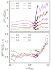Fig. A.1. Average density and mass radial profiles as a function of redshift. Upper panel: Ratio between the median shell density of clusters at the six redshifts z = 0.01, 0.21, 0.42, 0.62, 0.82, and 1.04 relative to z = 0.01. The color coding is shown in the legend. The thick section of each ratio shows the infalling shell (Sect. 4.1, Table 3). Bottom panel: Same as the upper panel but for the median cumulative mass profile.

In our sample, clusters at higher redshift are denser than their lower redshift counterparts, as expected. In the inner equilibrium region, $\lesssim R_{200c}^{3D}$ (Sect. 2.2, Fig. 1), the density ratios are roughly constant from one redshift bin to another. For r ≳ R_200c, the ratios reach a minimum and then increase. At larger cluster-centric distances, the ratios reach the ratios of the average cosmological mass density at the relevant epochs. Subtracting the cosmological mean density from the profiles does not change the qualitative behavior of the relative profiles. The cluster density dominates the total mass density for r ≲ (6 − 7)R_200c, a radius larger than the characteristic turnaround radius (Sect. 2.2).

The infalling shells are outside the virialized region (thick section in each curve of Fig. A.1). Because the cluster-centric radius of the radial velocity minimum decreases as redshift increases (see Sect. 2.2 and Table 3), the infalling shells are at different radii. The infalling shell volume decreases for shells nearer the cluster center. Furthermore, the shell thickness is also not constant. Taken together, these effects produce an increase of a factor of ∼2.0 in M_shell over the redshift range we probed.

The slightly different mass distributions that characterize the cluster samples as a function of redshift (Table 2) also affect the redshift dependence of M_shell. The bottom panel of Fig. A.1 shows the ratios of the median cumulative mass profiles. For the highest redshift clusters, the median mass profiles are ∼20% below the median profile at z = 0.01, decreasing the correlation between M_shell and redshift by a comparable fraction. This effect couples with the effects of the relative density profiles and produces a combined factor of an approximately 1.6 increase in M_shell over the range sampled by IllustrisTNG. In other words, the cluster mass distribution and the relative profiles as a function of redshift account for the lack of dependence of M_shell on redshift in the sample of clusters simulated with IllustrisTNG.

All Tables

All Figures

Fig. 1. Galaxy radial velocity profiles, infalling shells, and turnaround radii. The solid blue curves show the average galaxy radial velocity profiles for redshifts z = 0.01, z = 0.62, and z = 1.04 (left, middle, and right panels, respectively). The dashed blue curves show the Savitzky-Golay smoothed profiles based on a ten-bin window (Savitzky & Golay 1964). The shadowed region shows the error in the smoothed profile. The vertical black line shows the average turnaround radius based on the velocity profiles. In each panel the blue vertical band indicates the infalling shell with boundaries at cluster-centric radii where the velocity is 0.72vmin (Sect. 4).

In the text

	Fig. 2. Minimum radial velocity as a function of the cluster-centric radius of the minimum (color coded by redshift).
In the text

	Fig. 3. Relation between MAR and MARt. The curves show MAR3D(A)/MAR3D(A = 0.72) as a function of A in the range of 0.45 − 0.95 for six redshifts from z = 0.01 to z = 1.04. The error bar shows the median interquartile range of the ratio at A = 0.72.
In the text

Fig. 4. Relation between $M_{\mathrm{shell}}^{3\mathrm{D}}$ and $M_{200\mathrm{c}}^{3\mathrm{D}}$. The colored circles show $M_{\mathrm{shell}}^{3\mathrm{D}}$ as a function of $M_{200\mathrm{c}}^{3\mathrm{D}}$ in the three redshift bins z = 0.01, 0.62, and 1.04 (cyan, violet, and magenta, respectively). The squares with error bars indicate the median and interquartile range in eight fixed logarithmic mass bins. The lines show power law fits to the data.

In the text

Fig. 5. Relation between $M_{\mathrm{shell}}^{3\mathrm{D}}$ and redshift. The small circles show the $M_{\mathrm{shell}}^{3\mathrm{D}}$ of individual clusters as a function of redshift, color coded by $M_{200\mathrm{c}}^{3\mathrm{D}}$. The points include clusters over the entire redshift range. We introduced an artificial jitter on the exact redshifts to make the dependence of $M_{\mathrm{shell}}^{3\mathrm{D}}$ on $M_{200\mathrm{c}}^{3\mathrm{D}}$ more evident. The transparent black circles with error bars show the median and interquartile range of $M_{\mathrm{shell}}^{3\mathrm{D}}$ in each redshift bin.

In the text

	Fig. 6. Median and interquartile ranges of the ratio between the caustic and true Mshell as a function of redshift.
In the text

Fig. 7. Relation between tinf and $M_{200\mathrm{c}}^{3\mathrm{D}}$. The colored circles show tinf of individual clusters as a function of their mass $M_{200\mathrm{c}}^{3\mathrm{D}}$ in the three redshift bins z = 0.01, 0.62, and 1.04 (cyan, violet, and magenta, respectively). The squares with error bars indicate the median and the interquartile range in eight fixed logarithmic bins of mass. The lines show power law fits to the data.

In the text

	Fig. 8. Relation between MAR3D and $M_{200\mathrm{c}}^{3\mathrm{D}}$. The colored circles show MAR3D as a function of $M_{200\mathrm{c}}^{3\mathrm{D}}$ in the three redshift bins z = 0.01, 0.62, and 1.04 (cyan, violet, and magenta, respectively). The squares with error bars show the median and interquartile range in eight fixed mass bins. The lines show power law fits to the data.
In the text

	Fig. 9. Comparison between MARC and MAR3D. Upper panel: median true (blue squares) and caustic (red triangles) MARs as a function of redshift. The solid blue and dotted red error bars show the interquartile ranges of the true and caustic MARs, respectively. The black curve shows a fit to Eq. (8). Lower panel: median ratio (black dots) between the caustic and true MARs as a function of redshift.
In the text

Fig. 10. Comparison between our MARs and previously published results. Upper panel: squares show MAR3Ds from Fig. 8 as a function of $M_{200\mathrm{c}}^{3\mathrm{D}}$ and color coded by redshift, from dark blue to dark red as the redshift increases from bin to bin: z = 0.01, 0.21, 0.52, 0.82, and z = 1.04. The lines show MARs from merger trees by Fakhouri et al. (2010, dotted line) and by Diemer et al. (2017, solid line). Lower panel: squares again show the true MARs from TNG300-1 as a function of $M_{200\mathrm{c}}^{3\mathrm{D}}$. Triangles show the MAR3Ds from Pizzardo et al. (2022) as a function of $M_{200\mathrm{c}}^{3\mathrm{D}}$ in four redshift bins: z = 0.01, 0.19, 0.44, and z = 1.00. The stars show the MARs of ten observed stacked clusters from the HectoMAP survey (Pizzardo et al. 2022).

In the text

Fig. 11. Comparison between fits to our MARs and previously published fits. The solid, dotted, and dashed lines show the fit of the analytic relation proposed by Fakhouri et al. (2010) to the IllustrisTNG MARs (Eq. (8), see Sect. 5), the fit by Fakhouri et al. (2010), and the fit by Diemer et al. (2017), respectively, at z = 0.31. The shadowed turquoise band shows the typical 1σ IllustrisTNG scatter. The gray shadow indicates a similar assumed scatter for the merger tree models (gray bands).

In the text

Fig. 12. Comparison between MARs from galaxies and dark matter. Upper panel: blue squares (orange dots) and blue (orange) error bars show the median and the interquartile range of the true MARs based on galaxies (dark matter) as a function of redshift. Lower panel: points show the median ratio between the dark matter and galaxy MARs as a function of redshift. The dash-dotted line shows the median ratio.

In the text

Fig. A.1. Average density and mass radial profiles as a function of redshift. Upper panel: Ratio between the median shell density of clusters at the six redshifts z = 0.01, 0.21, 0.42, 0.62, 0.82, and 1.04 relative to z = 0.01. The color coding is shown in the legend. The thick section of each ratio shows the infalling shell (Sect. 4.1, Table 3). Bottom panel: Same as the upper panel but for the median cumulative mass profile.

In the text

References

- Achitouv, I., Wagner, C., Weller, J., & Rasera, Y. 2014, JCAP, 2014, 077 [Google Scholar]
- Adhikari, S., Dalal, N., & Chamberlain, R. T. 2014, JCAP, 11, 019 [Google Scholar]
- Allgood, B., Flores, R. A., Primack, J. R., et al. 2006, MNRAS, 367, 1781 [NASA ADS] [CrossRef] [Google Scholar]
- Bakels, L., Ludlow, A. D., & Power, C. 2021, MNRAS, 501, 5948 [NASA ADS] [CrossRef] [Google Scholar]
- Balcells, M., Benn, C. R., Carter, D., et al. 2010, in Ground-based and Airborne Instrumentation for Astronomy III, eds. I. S. McLean, S. K. Ramsay, & H. Takami, SPIE Conf. Ser., 7735, 77357G [NASA ADS] [Google Scholar]
- Baldi, M. 2012, MNRAS, 422, 1028 [NASA ADS] [CrossRef] [Google Scholar]
- Bardeen, J. M., Bond, J. R., Kaiser, N., & Szalay, A. S. 1986, ApJ, 304, 15 [Google Scholar]
- Bartelmann, M. 2010, CQG, 27, 233001a [NASA ADS] [CrossRef] [Google Scholar]
- Bett, P., Eke, V., Frenk, C. S., et al. 2007, MNRAS, 376, 215 [NASA ADS] [CrossRef] [Google Scholar]
- Bond, J. R., Cole, S., Efstathiou, G., & Kaiser, N. 1991, ApJ, 379, 440 [NASA ADS] [CrossRef] [Google Scholar]
- Bower, R. G. 1991, MNRAS, 248, 332 [NASA ADS] [CrossRef] [Google Scholar]
- Boylan-Kolchin, M., Springel, V., White, S. D. M., Jenkins, A., & Lemson, G. 2009, MNRAS, 398, 1150 [Google Scholar]
- Cataneo, M., & Rapetti, D. 2020, Modified Gravity: Progresses and Outlook of Theories, Numerical Techniques and Observational Tests (World Scientific), 143 [Google Scholar]
- Corasaniti, P. S., & Achitouv, I. 2011, Phys. Rev. Lett., 106, 241302 [NASA ADS] [CrossRef] [Google Scholar]
- Cornwell, D. J., Kuchner, U., Aragón-Salamanca, A., et al. 2022, MNRAS, 517, 1678 [NASA ADS] [CrossRef] [Google Scholar]
- Cornwell, D. J., Aragón-Salamanca, A., Kuchner, U., et al. 2023, MNRAS, 524, 2148 [NASA ADS] [CrossRef] [Google Scholar]
- Correa, C. A., Wyithe, J. S. B., Schaye, J., & Duffy, A. R. 2015a, MNRAS, 450, 1514 [NASA ADS] [CrossRef] [Google Scholar]
- Correa, C. A., Wyithe, J. S. B., Schaye, J., & Duffy, A. R. 2015b, MNRAS, 450, 1521 [NASA ADS] [CrossRef] [Google Scholar]
- Dalton, G. 2016, in Multi-Object Spectroscopy in the Next Decade: Big Questions, Large Surveys, and Wide Fields, eds. I. Skillen, M. Balcells, & S. Trager, ASP Conf. Ser., 507, 97 [Google Scholar]
- Dalton, G., Trager, S. C., Abrams, D. C., et al. 2012, in Ground-based and Airborne Instrumentation for Astronomy IV, SPIE, 8446, 220 [Google Scholar]
- Dalton, G., Trager, S., Abrams, D. C., et al. 2014, in Ground-based and Airborne Instrumentation for Astronomy V, eds. S. K. Ramsay, I. S. McLean, & H. Takami, SPIE Conf. Ser., 9147, 91470L [Google Scholar]
- Davis, M., & Peebles, P. J. E. 1983, ApJ, 267, 465 [Google Scholar]
- Davis, M., Efstathiou, G., Frenk, C. S., & White, S. D. M. 1985, ApJ, 292, 371 [Google Scholar]
- De Boni, C., Serra, A. L., Diaferio, A., Giocoli, C., & Baldi, M. 2016, ApJ, 818, 188 [NASA ADS] [CrossRef] [Google Scholar]
- De Simone, A., Maggiore, M., & Riotto, A. 2011, MNRAS, 418, 2403 [CrossRef] [Google Scholar]
- Diaferio, A. 1999, MNRAS, 309, 610 [CrossRef] [Google Scholar]
- Diaferio, A. 2004, Outskirts of Galaxy Clusters (IAU C195): Intense Life in the Suburbs No. 195 (Cambridge University Press) [Google Scholar]
- Diaferio, A., & Geller, M. J. 1997, ApJ, 481, 633 [NASA ADS] [CrossRef] [Google Scholar]
- Diemer, B. 2017, ApJS, 231, 5 [NASA ADS] [CrossRef] [Google Scholar]
- Diemer, B. 2018, ApJS, 239, 35 [NASA ADS] [CrossRef] [Google Scholar]
- Diemer, B., & Kravtsov, A. V. 2014, ApJ, 789, 1 [NASA ADS] [CrossRef] [Google Scholar]
- Diemer, B., Mansfield, P., Kravtsov, A. V., & More, S. 2017, ApJ, 843, 140 [NASA ADS] [CrossRef] [Google Scholar]
- Fakhouri, O., Ma, C.-P., & Boylan-Kolchin, M. 2010, MNRAS, 406, 2267 [Google Scholar]
- Gao, L., White, S. D. M., Jenkins, A., Stoehr, F., & Springel, V. 2004, MNRAS, 355, 819 [Google Scholar]
- Giocoli, C., Tormen, G., & Sheth, R. K. 2012, MNRAS, 422, 185 [NASA ADS] [CrossRef] [Google Scholar]
- Gunn, J. E., Gott, J., & Richard, I. 1972, ApJ, 176, 1 [Google Scholar]
- Hoekstra, H., Bartelmann, M., Dahle, H., et al. 2013, Space Sci. Rev., 177, 75 [NASA ADS] [CrossRef] [Google Scholar]
- Ivezić, Ž., Kahn, S. M., Tyson, J. A., et al. 2019, ApJ, 873, 111 [Google Scholar]
- Jenkins, A., Frenk, C. S., Pearce, F. R., et al. 1998, ApJ, 499, 20 [Google Scholar]
- Kaiser, N. 1984, ApJ, 284, L9 [NASA ADS] [CrossRef] [Google Scholar]
- Kasun, S., & Evrard, A. E. 2005, ApJ, 629, 781 [NASA ADS] [CrossRef] [Google Scholar]
- Lacey, C., & Cole, S. 1993, MNRAS, 262, 627 [NASA ADS] [CrossRef] [Google Scholar]
- Lau, E. T., Nagai, D., Avestruz, C., Nelson, K., & Vikhlinin, A. 2015, ApJ, 806, 68 [NASA ADS] [CrossRef] [Google Scholar]
- Laureijs, R., Amiaux, J., Arduini, S., et al. 2011, ArXiv e-prints [arXiv:1110.3193] [Google Scholar]
- Ludlow, A. D. 2009, PhD Thesis, University of Victoria, Canada [Google Scholar]
- Ludlow, A. D., Navarro, J. F., Boylan-Kolchin, M., et al. 2013, MNRAS, 432, 1103 [NASA ADS] [CrossRef] [Google Scholar]
- Mantz, A., Allen, S. W., Ebeling, H., & Rapetti, D. 2008, MNRAS, 387, 1179 [CrossRef] [Google Scholar]
- Mantz, A. B., Allen, S. W., Morris, R. G., et al. 2014, MNRAS, 440, 2077 [NASA ADS] [CrossRef] [Google Scholar]
- Mantz, A. B., von der Linden, A., Allen, S. W., et al. 2015, MNRAS, 446, 2205 [Google Scholar]
- Marshall, J., Bolton, A., Bullock, J., et al. 2019, BAAS, 51, 126 [Google Scholar]
- McBride, J., Fakhouri, O., & Ma, C.-P. 2009, MNRAS, 398, 1858 [NASA ADS] [CrossRef] [Google Scholar]
- More, S., Diemer, B., & Kravtsov, A. V. 2015, ApJ, 810, 36 [Google Scholar]
- Musso, M., Cadiou, C., Pichon, C., et al. 2018, MNRAS, 476, 4877 [Google Scholar]
- Nelson, D., Springel, V., Pillepich, A., et al. 2019, Comput. Astrophys. Cosmol., 6, 1 [NASA ADS] [CrossRef] [Google Scholar]
- O’Neil, S., Barnes, D. J., Vogelsberger, M., & Diemer, B. 2021, MNRAS, 504, 4649 [CrossRef] [Google Scholar]
- Pakmor, R., Springel, V., Coles, J. P., et al. 2023, MNRAS, 524, 2539 [NASA ADS] [CrossRef] [Google Scholar]
- Pillepich, A., Springel, V., Nelson, D., et al. 2018, MNRAS, 473, 4077 [Google Scholar]
- Pizzardo, M., Di Gioia, S., Diaferio, A., et al. 2021, A&A, 646, A105 [NASA ADS] [CrossRef] [EDP Sciences] [Google Scholar]
- Pizzardo, M., Sohn, J., Geller, M. J., Diaferio, A., & Rines, K. 2022, ApJ, 927, 26 [NASA ADS] [CrossRef] [Google Scholar]
- Pizzardo, M., Geller, M. J., Kenyon, S. J., Damjanov, I., & Diaferio, A. 2023, A&A, 675, A56 [NASA ADS] [CrossRef] [EDP Sciences] [Google Scholar]
- Power, C., Knebe, A., & Knollmann, S. R. 2011, MNRAS, 419, 1576 [Google Scholar]
- Press, W. H., & Schechter, P. 1974, ApJ, 187, 425 [Google Scholar]
- Ragone-Figueroa, C., Plionis, M., Merchán, M., Gottlöber, S., & Yepes, G. 2010, MNRAS, 407, 581 [NASA ADS] [CrossRef] [Google Scholar]
- Reiprich, T. H., Basu, K., Ettori, S., et al. 2013, Space Sci. Rev., 177, 195 [Google Scholar]
- Rines, K., & Diaferio, A. 2006, AJ, 132, 1275 [Google Scholar]
- Rines, K., Geller, M. J., Diaferio, A., & Kurtz, M. J. 2013, ApJ, 767, 15 [NASA ADS] [CrossRef] [Google Scholar]
- Rost, A., Kuchner, U., Welker, C., et al. 2021, MNRAS, 502, 714 [Google Scholar]
- Sartoris, B., Biviano, A., Fedeli, C., et al. 2016, MNRAS, 459, 1764 [Google Scholar]
- Savitzky, A., & Golay, M. 1964, J. Anal. Chem., 36, 1627 [Google Scholar]
- Schechter, P. L. 1980, AJ, 85, 801 [NASA ADS] [CrossRef] [Google Scholar]
- Serra, A. L., Diaferio, A., Murante, G., & Borgani, S. 2011, MNRAS, 412, 800 [NASA ADS] [Google Scholar]
- Sheth, R. K., & Tormen, G. 2002, MNRAS, 329, 61 [Google Scholar]
- Silk, J. 1974, ApJ, 193, 525 [NASA ADS] [CrossRef] [Google Scholar]
- Sohn, J., Geller, M. J., Hwang, H. S., et al. 2021a, ApJ, 909, 129 [NASA ADS] [CrossRef] [Google Scholar]
- Sohn, J., Geller, M. J., Hwang, H. S., et al. 2021b, ApJ, 923, 143 [NASA ADS] [CrossRef] [Google Scholar]
- Springel, V., White, S. D., Jenkins, A., et al. 2005, Nature, 435, 629 [Google Scholar]
- Springel, V., Pakmor, R., Pillepich, A., et al. 2018, MNRAS, 475, 676 [Google Scholar]
- Tamura, N., Takato, N., Shimono, A., et al. 2016, in Ground-based and Airborne Instrumentation for Astronomy VI, Int. Soc. Opt. Photonics, 9908, 99081M [Google Scholar]
- Tasitsiomi, A., Kravtsov, A. V., Gottlober, S., & Klypin, A. A. 2004, ApJ, 607, 125 [NASA ADS] [CrossRef] [Google Scholar]
- Umetsu, K. 2020, A&ARv, 28, 7 [Google Scholar]
- Umetsu, K., Broadhurst, T., Zitrin, A., et al. 2011, ApJ, 738, 41 [NASA ADS] [CrossRef] [Google Scholar]
- Umetsu, K., Zitrin, A., Gruen, D., et al. 2016, ApJ, 821, 116 [Google Scholar]
- van den Bosch, F. C. 2002, MNRAS, 331, 98 [CrossRef] [Google Scholar]
- van den Bosch, F. C., Tormen, G., & Giocoli, C. 2005, MNRAS, 359, 1029 [NASA ADS] [CrossRef] [Google Scholar]
- van den Bosch, F. C., Jiang, F., Hearin, A., et al. 2014, MNRAS, 445, 1713 [NASA ADS] [CrossRef] [Google Scholar]
- Vitvitska, M., Klypin, A. A., Kravtsov, A. V., et al. 2002, ApJ, 581, 799 [NASA ADS] [CrossRef] [Google Scholar]
- Villumsen, J. V., & Davis, M. 1986, ApJ, 308, 499 [NASA ADS] [CrossRef] [Google Scholar]
- Walker, S., Simionescu, A., Nagai, D., et al. 2019, Space Sci. Rev., 215, 1 [CrossRef] [Google Scholar]
- Wechsler, R. H., Bullock, J. S., Primack, J. R., Kravtsov, A. V., & Dekel, A. 2002, ApJ, 568, 52 [NASA ADS] [CrossRef] [Google Scholar]
- White, M. 2002, ApJS, 143, 241 [Google Scholar]
- White, S. D. M., & Rees, M. J. 1978, MNRAS, 183, 341 [Google Scholar]
- White, S. D. M., Davis, M., Efstathiou, G., & Frenk, C. S. 1987, Nature, 330, 451 [NASA ADS] [CrossRef] [Google Scholar]
- Xhakaj, E., Leauthaud, A., Diemer, B., & Behroozi, P. 2019, Res. Notes Am. Astron. Soc., 3, 169 [Google Scholar]
- Zhang, Y. Y., Finoguenov, A., Böhringer, H., et al. 2004, A&A, 413, 49 [NASA ADS] [CrossRef] [EDP Sciences] [Google Scholar]
- Zhang, J., Ma, C.-P., & Fakhouri, O. 2008, MNRAS, 387, L13 [CrossRef] [Google Scholar]