| Issue |
A&A
Volume 632, December 2019
|
|
|---|---|---|
| Article Number | A101 | |
| Number of page(s) | 23 | |
| Section | Interstellar and circumstellar matter | |
| DOI | https://doi.org/10.1051/0004-6361/201935409 | |
| Published online | 10 December 2019 | |
Chemical and kinematic structure of extremely high-velocity molecular jets in the Serpens Main star-forming region★
1
Leiden Observatory, Leiden University,
PO Box 9513,
2300 RA
Leiden,
The Netherlands
e-mail: This email address is being protected from spambots. You need JavaScript enabled to view it.
2
National Astronomical Observatory of Japan, NAOJ Chile Observatory,
Alonso de Córdova 3788, Office 61B,
Vitacura
763 0422,
Santiago,
Chile
3
Joint ALMA Observatory,
Alonso de Córdova 3107,
Vitacura
763 0355,
Santiago,
Chile
4
Centre for Star and Planet Formation, Niels Bohr Institute and Natural History Museum of Denmark, University of Copenhagen,
øster Voldgade 5-7,
1350
Copenhagen K,
Denmark
5
National Radio Astronomy Observatory,
Charlottesville,
VA
22903,
USA
6
European Southern Observatory,
Alonso de Córdova 3107,
Vitacura,
Santiago,
Chile
7
AIM, CEA, CNRS, Université Paris-Saclay, Université Paris Diderot,
Sorbonne Paris Cité,
91191
Gif-sur-Yvette,
France
8
Max-Planck-Institut für Extraterrestrische Physik,
Giessenbachstrasse 1,
85748
Garching,
Germany
Received:
5
March
2019
Accepted:
16
October
2019
Abstract
Context. Outflows are one of the first signposts of ongoing star formation. The fastest molecular component of protostellar outflows, extremely high-velocity (EHV) molecular jets, are still puzzling since they are seen only rarely. As they originate deep inside the embedded protostar-disk system, they provide vital information about the outflow-launching process in the earliest stages.
Aims. The first aim is to analyze the interaction between the EHV jet and the slow outflow by comparing their outflow force content. The second aim is to analyze the chemical composition of the different outflow velocity components and to reveal the spatial location of molecules.
Methods. The Atacama Large Millimeter/submillimeter Array 3 mm (Band 3) and 1.3 mm (Band 6) observations of five outflow sources at 0.′′3 – 0.′′6 (130–260 au) resolution in the Serpens Main cloud are presented. Observations of CO, SiO, H2CO, and HCN reveal the kinematic and chemical structure of those flows. The following three velocity components are distinguished: the slow and the fast wing, and the EHV jet.
Results. Out of five sources, three have the EHV component. The comparison of outflow forces reveals that only the EHV jet in the youngest source, Ser-emb 8 (N), has enough momentum to power the slow outflow. The SiO abundance is generally enhanced with velocity, while HCN is present in the slow and the fast wing, but disappears in the EHV jet. For Ser-emb 8 (N), HCN and SiO show a bow-shock shaped structure surrounding one of the EHV peaks, thus suggesting sideways ejection creating secondary shocks upon interaction with the surroundings. Also, the SiO abundance in the EHV gas decreases with distance from this protostar, whereas it increases in the fast wing. H2CO is mostly associated with low-velocity gas, but, surprisingly, it also appears in one of the bullets in the Ser-emb 8 (N) EHV jet. No complex organic molecules are found to be associated with the outflows.
Conclusions. The high detection rate suggests that the presence of the EHV jet may be more common than previously expected. The EHV jet alone does not contain enough outflow force to explain the entirety of the outflowing gas. The origin and temporal evolution of the abundances of SiO, HCN, and H2CO through high-temperature chemistry are discussed. The data are consistent with a low C/O ratio in the EHV gas versus a high C/O ratio in the fast and slow wings.
Key words: astrochemistry / ISM: jets and outflows / techniques: interferometric / stars: protostars / submillimeter: ISM / line: profiles
The datacubes are also available at the CDS via anonymous ftp to cdsarc.u-strasbg.fr (130.79.128.5) or via http://cdsarc.u-strasbg.fr/viz-bin/cat/J/A+A/632/A101
NAOJ Fellow.
© ESO 2019
1 Introduction
Spectacular outflows are one of the crucial signposts of ongoing star formation. Outflows are invoked to release angular momentum, enabling a continuous flow of matter onto the disk and the young star (e.g., Frank et al. 2014). Their feedback from small to large scales can have a profound impact on the evolution of both the protostar and the entire parent star-forming region (e.g., Arce & Sargent 2006; Plunkett et al. 2013). Thus, probing the youngest and most powerful outflow sources is crucial for understanding the interactions between the outflows and their surroundings.
While the molecular emission from a typical protostellar outflow usually appears as slow and wide-angle entrained gas, there is a peculiar group of sources with high-velocity collimated molecular emission. The extremely high-velocity (EHV) molecular jets (v > 30 km s−1) are found toward the youngest protostars (e.g., Bachiller et al. 1990; Bachiller 1996) in the Class 0 stage (André et al. 1993). They were first detected as spectral features, high-velocity peaks detached from the low-velocity outflow wings (Bachiller et al. 1990), and subsequently spatially resolved as discrete bullets embedded in a cocoon of low-velocity gas (e.g., Santiago-García et al. 2009; Hirano et al. 2010). These “bullets” are thought to arise from the variability of the outflow activity, which is possibly related to the variability of the accretion processes itself (Raga et al. 1993). In the deeply embedded stage, EHV molecular jets have been observed at submillimeter wavelengths (e.g., Bachiller et al. 1994; Tafalla et al. 2004), as well as in far-infrared (IR) observations (Kristensen et al. 2012; Mottram et al. 2014). They appear to be quite rare. In a survey of 29 protostars with Herschel Space Observatory/Heterodyne Instrument for the Far-Infrared (HIFI), water bullets were detected in only four sources, all of them being Class 0 (Kristensen et al. 2012). Thus, EHV jets are thought to be associated exclusively with very young sources.
Apart from the spatial and spectral characteristics of the EHV jets relative to low-velocity outflows, it appears that their chemical composition is significantly different from that of the slow outflow. In observations with the IRAM-30 m of two young outflows with EHV jet components, Tafalla et al. (2010) show that the molecular jets are more oxygen-rich compared to the slow and the fast wing component of the molecular outflow. The molecular jets are prominently seen in species, such as SiO (see also Guilloteau et al. 1992), SO, CH3OH, and H2CO, whereas emission from molecules like HCN and CS, which tend to be present in the slow and the fast wing, is missing at the highest velocities. These led Tafalla et al. (2010) to define three distinct velocity components: the slow and the fast wing, and the EHV jet (see Sect. 3.2). These studies presented spectrally resolved line profiles of different molecules, but their spatial location remains unclear. To date, only CO and SiO have been studied at high spatial resolution within the EHV jets (e.g., Lee et al. 2008; Santiago-García et al. 2009; Hirano et al. 2010; Codella et al. 2014; Hull et al. 2016). It is still not well understood what the spatial distribution of other molecules is in the different kinematic components of the outflow.
Additional important information on molecular jets and outflows comes from observations with the HIFI instrument (de Graauw et al. 2010) on board Herschel (Pilbratt et al. 2010) on scales of 1.′′–40′′. Many water and high-J CO transitions probing warm shocked gas show complex line profiles that can be decomposed in two main velocity components. The kinematic and chemical signatures of those components are universal for all protostars, from low to high mass (Kristensen et al. 2012; Mottram et al. 2014; San José-García et al. 2016): a broad component (FWHM > 20 km s−1), and an offset component (20 > FWHM > 5 km s−1), which is usually blue-shifted with respect to the systemic velocity up to a few km s−1. The CO excitation temperatures in the broad component are typically 300 K in the broad component and 700 K in the offset component. EHV bullets are also seen in HIFI line profiles as discrete peaks that are detached from the main line profile; however, as noted above, these only appear in a few sources. The spatial origin of those components can potentially be revealed with spectrally and spatially resolved Atacama Large Millimeter/submillimeter Array (ALMA) observations of low-J CO and other molecules. ALMA’s high spatial resolution is needed since the water analysis suggests that its emission originates from structures that are only a few hundred au in size. This is much smaller than the region encompassed by the HIFI beam at distances of nearby star-forming regions (Mottram et al. 2014).
Here we target three protostars in the Serpens Main region at a distance of 436 pc (Ortiz-León et al. 2017), namely, the Serpens SMM1 (hereafter referred to as SMM1), S68N, and Ser-emb 8 (N) protostellar systems. SMM1 is directly between a low and intermediate mass protostar (100 L⊙ ; Kristensen et al. 2012), and it is known to host a massive disk-like structure (Hogerheijde et al. 1999; Enoch et al. 2010). The SMM1 source was discovered as a multiple system in the continuum observations (Choi 2009) as confirmed by the observations of the atomic jet (Dionatos et al. 2014). More recently, resolving the system with ALMA unveiled a total of five protostellar components (Hull et al. 2017) within a 2000 au radius, three of which show outflows (labeled a, b, and d in Fig. 1). S68N and Ser-emb 8 (N) are deeply embedded protostars separated by 5000 au (Fig. 1b), and both power outflows (Hull et al. 2014). The chemical structure of Serpens Main on cloud scale has been studied in detail by McMullin et al. (1994, 2000) and Kristensen et al. (2010). A summary of the sources is provided in Table 1.
ALMA observations of CO 2−1 and SiO 5−4 reveal EHV jets toward the SMM1-a and SMM1-b sources in CO, which are both asymmetric, and only redshifted emission is detected at high velocities. SMM1-b additionally shows EHV emission in SiO (Hull et al. 2016, 2017).
In this paper we use ALMA to resolve, both spectrally and spatially, the emission from different molecules. This allow us not only to distinguish different kinematic components of the outflows and jets from protostars but also to link them to the specific physical components of the system, such as entrained gas, outflow cavity walls, or the protostellar jet.
2 Observations
ALMA observations of four molecular transitions, CO 2−1, SiO 5−4, H2CO 303 − 202 in Band 6 (ALMA project 2013.1.00726.S; PI: C. Hull) and HCN 1−0 observed in Band 3 (ALMA project 2016.1.00710.S; PI: C. Hull) are presented. The synthesized beam of the observations is between ~0.′′3 and ~0.′′6, corresponding to 130–260 au at the distance to Serpens Main. The largest recoverable scale in the data is ~.′′and ~ 1.′′(2150 and 4960 au) for Band 3 and Band 6, respectively. The spectral resolution of the observations differs between the spectral windows, ranging from 0.04–0.3 km s−1. For both bands, only 12-m array data were used. The Band 6 data were obtained in two configurations (C43-1 and C43-4 with resolutions of 1.′′1 and 0.′′3, respectively), and the final images were produced from the combined datasets.
After obtaining the C43-4 configuration data, it became apparent that SiO and H2CO emission is present atvelocities extending further than the spectral setup. To capture the emission at high-velocities, the spectral configuration for SiO and H2CO was changed for the compact C43-1 configuration. Thus the SiO and H2CO emission at the highest velocities (>40 km s−1 for SiO and >25 km s−1 for H2CO in both the redshifted and blueshifted direction with respect to the systemic velocity of 8.5 km s−1) are only available at lower spatial resolution.
Continuum images were obtained from the dedicated broadband spectral windows and line-free channels. Self-calibration on continuum data was performed, and solutions were transferred to the emission line measurement sets. The line data were then continuum subtracted. The imaging was performed with the Common Astronomy Software Application (CASA) v. 5.1.0 (McMullin et al. 2007) tclean task with masked regions selected by hand for each line. Data were imaged with Briggs weighting = 0.5 and re-binned to 0.5 km s−1. Due to the large extent and complicated structure of the emission lines, the multiscale option in tclean was used for the lines, and the scales were manually adjusted for each line. Information about the observations is summarized in Table C.1.
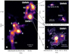 |
Fig. 1 Left: JCMT/SCUBA 850-μm map of Serpens Main region with numbers corresponding to SMM sources as classified by Davis et al. (1999). Contours are [3, 6, 12, 20, 40] × 0.50 mJy arcsec−2. Beam of the JCMT observations of 1.′′is indicated in the bottom-left corner. Right: ALMA 1.3 mm continuum of targeted protostars. For SMM9, field contours are [3, 6, 9, 12] × 0.53 mJy beam−1 and for SMM1 field contours are [3, 4, 5, 6, 9, 15, 40, 50] × 0.62 mJy beam−1. Synthesized beams of the ALMA observations are 0.′′35 × 0.′′33 for the SMM9 field and 0.′′36 × 0.′′30 for the SMM1 field. |
Targeted protostars.
3 Results
3.1 Images of outflows
The highest resolution and sensitivity observations of the S68N and Ser-emb 8 (N) molecular outflows taken to date are presented here. For SMM1, H2CO, and HCN, emission is shown in addition to the CO and SiO outflow presented in previous papers (Hull et al. 2016, 2017). Figures 2 and 3 show the integrated emission maps of CO, SiO, H2CO, and HCN for all five sources. Various other molecules were detected as well in the ALMA observations (e.g., DCO+, C18O, and complex organic molecules; Tychoniec et al. 2018). Those molecules either trace the cold quiescent envelope or the warm inner envelope, but they do not show the outflow components; thus, they are not further discussed here.
Ser-emb 8 (N) (Fig. 2) shows a relatively symmetric outflow morphology in CO. It has a very small opening angle of 25°, which was measured as an angle between the outflow cavity walls seen at the low-velocity CO. SiO emission toward this source traces both the central, most collimated part of the outflow, and the bow-shock structure at the redshifted part of the outflow, which are also clearly seen in the HCN. The structure is not so clear on the blueshifted side, although HCN is mostly present off of the main axis of the outflow there, while there is no clear evidence for a blueshifted bow-shock from SiO emission. H2CO is enhanced at the bow-shock position in the redshifted part of the outflow.
S68N has an outflow with a wide opening angle of 50°, although the cavity walls do not seem well defined for this source (Fig. 3). The morphology of the outflow is similar in all molecules, but it can be noticed that peaks of the SiO emission generally appear in regions with weaker CO emission. There seems to be a narrow on-axis ridge on the redshifted side of the S68N outflow where both SiO and HCN emission peaks. This is in contrast to H2CO, which emits mostly off-axis.
The SMM1-a outflow has an asymmetric structure in CO, which is comprised of misaligned blue- and redshifted lobes with respect to each other (30° difference in position angles) and the following different opening angles: 65° and 35° for red and blueshifted sides, respectively (Fig. 3). Other molecules are seen close to the protostar rather than throughout the full extent of the outflow, for example, SiO is only found very close to the protostar and only on the redshifted side, furthermore, H2CO and HCN are seen tracing the innermost regions of the outflow with irregular morphologies.
SMM1-b has an outflow with consistent position angles on both sides, but the redshifted part is much brighter in both CO and SiO (Fig. 3). The CO outflow has a moderate opening angle of 45°; the blueshifted part of the SiO emission is only detected several thousands of au away from the source as a clump of emission. This is very different from the bright, highly-collimated structures with several well-defined bullets on the redshifted side of the jet. HCN and H2CO are only faintly detected toward SMM1-b at low-velocities.
The SMM1-d outflow has a peculiar morphology (Fig. 3); the redshifted side is seen in three distinct clumps starting as far as 3000 au away from the SMM1-d protostar (Hull et al. 2017), while no blueshifted side is observed. The CO emission peaks at the nearest clump while the SiO, HCN, and H2CO peak in the most distant one.
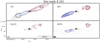 |
Fig. 2 Integrated intensity maps of CO 2−1, SiO 5− 4, H2CO 303−202, and HCN 1−0 overlaid on the Band 6 (Band 3 for HCN) continuum in grayscale for Ser-emb 8 (N). The emission is integrated from the inner boundary of the slow wing component to the outer boundary of the EHV component as listed in Table 2 for the red and blueshifted emission. The exceptions are SiO and H2CO maps where only the channels obtained at high spatial resolution are plotted (<26 km s−1 for H2CO and <40 km s−1 for SiO). The synthesized beam size of the continuum images is 0.′′35 × 0.′′33 for Band 6 and 0.′′79 × 0.′′64 for Band 3; for spectral lines it is 0.′′53 × 0.′′45 (CO), 0.′′55 × 0.′′45 (SiO), 0.′′53 × 0.′′44 (H2CO), and 0.′′60 × 0.′′56 (HCN). The beam size of the Band 6 spectral line is presented in the bottom-left corner of the H2CO map and in HCN map for Band 3. Contour levels are [3, 6, 9, 15, 20, 40, 60, 80, 100] for CO, SiO, H2CO, and redshifted HCN, and [2, 3, 5, 6, 12] for blueshifted HCN, which were multiplied by rms value of moment 0 maps. The rms values for the blueshifted and redshifted side of the outflow in K km s−1 is as follows: CO [19.7, 14.4], SiO [2.2, 2.5], H2CO [2.8, 2.1], and HCN [9.3, 12.2]. Black ellipses indicate regions from which spectra were extracted for Figs. 4 and B.1. |
3.2 Velocity regimes
The high spectral resolution and high sensitivity observations of ALMA allow for the analysis of the different velocity components present in the outflows. Tafalla et al. (2010) define three velocity components in molecular outflows as follows: the slow wing is seen as a typical Gaussian profile and the fast wing shows up as a broad component added to this profile; and the transition between the two is smooth. The EHV component appears as a discrete peak at high velocities and is clearly separated from the wing profile.
To define boundaries between the velocity regimes, especially to distinguish the slow from the fast wing, the examination of multiple molecules is needed. We note that C18O spectra within the Band 6 observations have been used to set constraints on possible contamination by the envelope emission in the outflow measurements, even though most of the envelope emission should be resolved out. Spectra of C18O of regions outside the outflow positions were used to assess, with the naked eye, the velocity at which C18O is still significant. Those values are set as the inner velocity limit for the slow wing.
Tafalla et al. (2010) identify the transition between slow and fast wing by a decrease of intensity of H2CO emission and an enhancement of SiO and HCN, relative to CO; where possible, the same criteria are used here. Defining the EHV regime is more straightforward as it is the beginning of the increasing CO and SiO flux at high velocities. Figure 4 shows spectra used to define the velocity regimes in Ser-emb 8 (N). Table 2 summarizes the velocity borders defined for each source.
Out of the five outflow sources observed, the EHV component is detected toward three sources. This is remarkable, as it is considered to be a rare phenomenon. The new detection of the Ser-emb 8 (N) high-velocity molecular jet, along with further analysis of EHV jets toward SMM1-a and SMM1-b (Hull et al. 2016, 2017), is presented here.
Figure 5 shows intensity maps of CO (2− 1) integrated over velocity regimes defined in the previous section. Ser-emb 8 (N) has a high degree of symmetry between red and blueshifted emission at high velocities, with several peaks of emission, occurring at similar distances from the protostar on both sides. Three main clumps of EHV emission can be distinguished at 1500, 4000, and 6000 au away from the central protostar, although each of those clumps can be split into a more complex structure.
A similar bullet-like structure is observed toward the SMM1-b source in its redshifted jet, with bullets at roughly 1000, 3000, 5000, and 7000 au. The redshifted bullets seem to have only a single blueshifted counterpart - the furthermost EHV component at ~ 7000 au (Fig. B.3).
The EHV component from SMM1-a is very different from that of the first two jets described. It resembles a continuous stream emerging very close to the protostar, rather than forming discrete bullets. Hints of redshifted EHV emission that are further away are present as far as 7000 au from the protostar, although they are significantly off-axis compared with the stream that is close to the protostar; this may suggest precession, as discussed by Hull et al. (2016). No corresponding blueshifted EHV emission is seen toward this source, which is in contrast to the slow and fast wing gas (Fig. B.2).
S68N shows no signs of the EHV component. (Fig. B.5). In the case of the SMM1-d outflow (Fig. B.4), it is difficult to assign the velocity components described above because almost all emission is confined to the low-velocity stream. SiO and HCN seem to follow CO in the spectral profile, and no enhancement is seen at higher velocities, but the CO profile appears broad and therefore slow and fast wing components are assigned. EHV emission is not present toward this source.
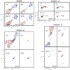 |
Fig. 3 Similar to Fig. 2, but for remaining sources. S68N: contour levels are [3, 6, 9, 15, 20, 40, 60, 80, 100] for CO and HCN; [3, 8, 15, 30, 45] for SiO; and [3, 5, 9, 15, 20, 40] for H2CO, which were multiplied by the rms value of moment 0 maps. The rms values for the blueshifted and redshifted side of the outflow, in Kkm s−1: CO [19.5, 14.1], SiO [1.6, 1.9], H2CO [3.2, 2.0], and HCN [9.4, 12.7]. SMM1-a: contour levels are [3, 6, 9,15, 20, 40, 60, 80, 100] for all molecules, which were multiplied by the rms value of moment 0 maps. The rms values for the blueshifted and redshifted side of the outflow, in K km s−1 : CO [20.2, 20.6], SiO [3.6, 4.0], H2CO [2.0, 2.9], and HCN [7.5, 11.5]. SMM1-b: contour levels are [3, 6, 9, 15, 20, 40, 60, 80, 100] for CO, [3, 9, 36] for SiO, and [3, 5] for H2CO and HCN, which were multiplied by the rms value of moment 0 maps. The rms values for the blueshifted and redshifted side of the outflow, in K km s−1 : CO [18.7, 20.3], SiO [3.6, 4.0], H2CO [1.9, 2.9], and HCN [7.4, 11.5]. SMM1-d: only redshifted moment 0 map is presented as no blueshifted component has been detected toward this source. Contour levels are [3, 6, 9, 15, 20, 40, 60, 80, 100] for CO and HCN, [3, 12, 36] for SiO, and [2, 3] for H2CO, which were multiplied by the rms value of moment 0 maps. The rms values in K km s−1 are: CO [20.1], SiO [3.3], H2CO [2.7], and HCN [9.1]. Black ellipses indicate regions from which spectra were extracted for Fig. B.1. |
3.3 Chemical abundances in velocity components
Probing the composition of the wind at different velocities can shed light on physical conditions within the outflows, since a change in velocity also triggers a change in temperature and density. Moreover, a contrast between the chemical composition of wing and jet components can also point to a different physical origin of the outflowing gas (Tafalla et al. 2010), and thus help us to understand the mechanism of the EHV jet formation and its interaction with entrained and quiescent gas.
Boundary velocities of different components.
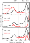 |
Fig. 4 Spectra of CO (black) and SiO, H2CO, and HCN (red) for selected part of blueshifted part of Ser-emb 8 (N) outflow, indicated in Fig. 2. The dashed lines show boundaries between different velocity components. Full set of spectra for the other sources is shown in Fig. B.1. |
3.3.1 Analysis method
The emission from each pixel inside a region defined by hand was summed in order to measure the abundances in each flow. The region was defined based on the extent of the low-velocity CO emission for the red and blueshifted parts of the outflow separately. These regions were then consistently used for all molecules and all velocity regimes. We calculated an integrated intensity of every pixel within the region, with the integration going from fixed vin to vout specified for each velocity regime (see Table 2).
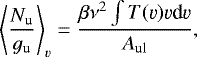
Assuming that the emission is optically thin, the column density of the molecule in each pixel is computed as:
 (1)
(1)
where β = 8πk∕hc2, ν is frequency, Aul is the Einstein coefficient of a transition, gu is the degeneracy of the transition, and T(v) is an intensity of the emission in Kelvin in a single channel of velocity, v, with dv being a width of a channel. For a given excitation temperature, the column density of the molecule in a pixel is then:
![Mathematical equation: \begin{equation*} N_{\textrm{tot}} = N_{\textrm{u}} \times Q(T)\Big[g_{\textrm{u}}e^{-E_{\textrm{u}}/kT}\Big], \end{equation*}](/articles/aa/full_html/2019/12/aa35409-19/aa35409-19-eq2.png) (2)
(2)
where Q(T) is the partition function at the assumed excitation temperature. Since only a single transition of each molecule was observed, it is not possible to derive an excitation temperature from these data. The CO excitation temperature is set to 75 K, based on statistics of excitation temperatures for low-mass protostars (Yıldız et al. 2015; van Kempen et al. 2009), which show that the bulk of the low-J CO emission can be fit with this value.
The assessment of excitation temperatures for other molecules is not straightforward. Tafalla et al. (2010) performed an LTE analysis of all molecules included in this work for several transitions and obtained a very low values of Tex of ~ 7 K. However, their analysis was performed using low-energy transitions. Nisini et al. (2007) show, based on SiO observations for a broader range of Eup, that the conditions in the outflow may exhibit much higher kinetic temperatures. Their work shows an increase in temperature (up to 500 K) and density (up to 106 cm−3) for the high-velocity jet, which is consistent with the values derived from CO Herschel data (Karska et al. 2018). For SiO, H2CO, and HCN we ran RADEX (van der Tak et al. 2007) calculations to constrain excitation temperatures under the conditions expected in the protostellar outflow (nH2 = 104 –106 cm−3; Tkin = 75–700 K; Δv = 10 km s−1). The extreme excitation temperatures found this way (low and high, see the column Tex in Table 3) are used to calculate the column densities and associated uncertainties for those molecules. The excitation temperatures of the SiO, H2CO, and HCN are lower than the expected kinetic temperatures as the critical density of the transitions are high, see column ncrit in Table 3. The low critical density of the CO transition justifies the assumption that its excitation temperature is equal to the kinetic temperature.
Optically thin emission is assumed for all the molecules. SiO emission has been suggested to be optically thick for the outflowing gas (Lee et al. 2008; Cabrit et al. 2012). Our calculations with RADEX show that within the conditions expected in the outflows, the SiO 5–4 emission reaches τ ~ 0.1 only for high gas densities nH2 = 106 cm−3 at low temperatures Tkin = 75 K for the column densities inferred here (Sect. 3.3.2; Tables C.2–C.6. High optical depths are only found with our RADEX calculations for much narrower linewidths, but all the lines observed within our sample are broad.
The H2CO can become optically thick for high Tkin = 700 K; regardless of gas density. Therefore if the emission comes from the highest velocity material, the abundance of H2CO may be underestimated. For the column densities we infer that HCN 1–0 emission seems to be optically thick regardless of the conditions in the shock, and thus abundances of this molecule should be treated as lower limits.
For CO, our RADEX calculations show that τ ~ 0.3 for the low-velocity gas with Tkin ~ 75 K. Dunham et al. (2014) suggest that CO lines can become optically thick at low velocities (< 2 km s−1). By excluding channels at the lowest velocities using C18O as a tracer of the dense gas, we mostly probe the optically thin gas as the opacity rapidly decreases with velocity for CO wings (Yıldız et al. 2015; van der Marel et al. 2013; Zhang et al. 2016).
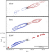 |
Fig. 5 Integrated intensity maps of CO for different velocity regimes overlaid on Band 6 continuum in grayscale for Ser-emb 8 (N). The emission is integrated over the velocities listed in Table 2. The synthesized beams of the CO (red) and continuum (black) are showed in bottom-left corner of EHV plot with sizes 0.′′35 × 0.′′33 and 0.′′55 × 0.′′45 for continuum and CO, respectively. The contours are [3, 6, 9, 15, 20, 40, 60, 80, 100] times the rms value. The rms values for each velocity channel, which are blueshifted and redshifted in K km s−1, are slow [18.3, 13.7], fast [3.1, 4.5], EHV [1.7, 1.4]. |
Outflow molecules.
3.3.2 Column densities and abundances
After calculating the column density in each pixel, the average of the column density within the pre-defined region was calculated from only those pixels with a signal above 3σ. Calculated values for each molecule are summarized in Tables C.2–C.6, where the boundary values calculated for the minimum and maximum Tex are reported.
Abundances shown in Figs. 6 and 7 were obtained from the column density calculated for a mean temperature between the two extreme Tex reported for each molecule in Table 3. To obtain the abundance with respect to CO, this column density was divided by the column density of CO calculated for T = 75 K. The CO column density was measured only in the region in which the emission from both molecules is above 3σ.
Figure 6 shows that the molecular abundances relative to CO change with velocity for each source. SiO increases in relative abundance from the slow to the fast wing for the redshifted SMM1-b outflow and both sides of the Ser-emb 8 (N) outflow. For the blueshifted Ser-emb 8 (N) flow, the abundance continues to rise toward the EHV regime, while it remains relatively constant for redshifted SMM1-b and Ser-emb 8 (N). H2CO is primarily associated with low-velocity gas, and it disappears in the fast wing for all sources. The only outflow to have EHV H2CO emission is the blueshifted part of the Ser-emb 8 (N) outflow, where H2CO reappears inthe EHV jet with a relative abundance to CO around two times higher than in the slow gas. HCN is present in most of the outflows in both the slow and fast wing, but it is never present in the EHV gas.
Even within the same velocity regime, the emission may come from different spatial regions, thus the analysis of the abundances over the entire outflow introduces additional uncertainties. Therefore, for the clearest case of the EHV jet, Ser-emb 8 (N), we also measured the molecular abundances along the different positions of the outflow in order to probe local abundances.
Figure 7 shows molecular abundances measured at three different positions on both sides of the Ser-emb 8 (N) outflow with regions defined appropriately to capture all of the lower-resolution SiO emission at the position. A remarkably similar behavior of SiO relative to CO can be noted on both sides of the outflow. For the fast wing gas, SiO abundance increases with distance from the protostar up to the bullet at 4000 au and then it disappears. In the EHV gas, the highest SiO abundance is observed close to the protostar, and then it drops with distance to the protostar by more than an order of magnitude.
The furthermost region, associated with the CO bullet, is depleted in all of the molecules except CO. The intermediate region at 4000 au appears as the most abundant in molecules, with HCN and SiO increasing for the slow and the fast wing. The H2CO abundance is similar in the regions where it is detected.
To highlight the variations in the abundance ratios, maps of the SiO to CO ratio in the blueshifted part of the Ser-emb 8(N) are shown in Fig. 8. Only the blueshifted part is shown as an example since the significant part of the redshifted EHV jet in SiO has been observed only at lower spatial resolution. It is clear that for the fast wing, the SiO/CO ratio peaks at a significant distance from the protostar (3000 au; corresponding to dynamical age of 500 yr for a 30 km s−1 outflow). In the EHV jet, the SiO/CO ratio peaks at a similar distance as in the fast wing and then decreases.
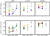 |
Fig. 6 Molecular abundances with respect to CO scaled by 104 for blueshifted (top) and redshifted (bottom) part of outflow for all sources. Gray triangles represent upper limits. Points on the plot show values calculated for the mean Tex of the range defined for each molecule, see Table 3. Error bars represent the column densities calculated for minimum and maximum values of the excitation temperature. To obtain the abundanceof the given molecule, the column density was divided by the CO column density (for Tex = 75 K.) measured in the region in which the emission from the molecule was above 3σ. The HCN emission is likely optically thick and therefore the abundance should be treated as a lower limit. |
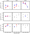 |
Fig. 7 Molecular abundances with respect to CO scaled by 104 for Ser-emb 8 (N). The distance from the protostar is on the x-axis. Panels from left to right are for the slow wing, the fast wing, and the EHV component. The abundances measured for three different regions along the outflow are shown for blueshifted and redshifted parts of the outflow separately. Abundances are measured in the same manner as in Fig. 6. The HCN emission is likely optically thick and therefore the abundance should be treated as a lower limit. |
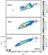 |
Fig. 8 Maps of SiO/CO ratio for blueshifted part of Ser-emb 8(N) outflow for each velocity component. For the EHV component, only the channels for which SiO emission was obtained at high spatial resolution are taken into account (<40 km s−1). The synthesized beams of the CO (red) and continuum (black) are shown in the bottom-left corner of EHV plot with sizes 0.′′35 × 0.′′33 and 0.′′55 × 0.′′45 for continuum and CO, respectively. The black contours show 1.3 mm continuum emission. |
3.4 Outflow force
Detection of the EHV molecular jets provides a unique opportunity to probe the fastest and the most collimated part of the outflowing material. Quantifying the distribution of kinetic energy and mass among the different velocity components sheds light on their kinematic relationship, specifically determining if the jet is the driving force of the slow outflow.
The mass of the gas must be derived from the number of molecules (see Sect. 3.3). The area of the pixel, times the total number of molecules within pixel Ntot, times the ratio of H2 ∕CO = 1.2 × 10⁴ (Frerking et al. 1982) with a molecular weight μ = 2.8 that takes helium into account (Kauffmann et al. 2008), times the mass of the hydrogen atom mH gives the amount of gas mass in a pixel (Yıldız et al. 2015):
 (3)
(3)
The momentum of the outflowing material can then be defined accordingly:
 (4)
(4)
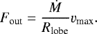
We define the distance from the protostar to the edge of the integration region as Rlobe. It is important to note that the area of the ALMA observations in all cases, except for SMM1-d and Ser-emb 8 (N), does not cover the full extent of the outflows, as evident in single dish observations (Dionatos et al. 2010; Yıldız et al. 2015). For that reason, parameters like outflow mass or momentum do not provide information about the overall gas mass and kinetic energy content in the flow, but they are rather local values or lower limits to those; the outflow force, on the other hand, is dependent on Rlobe and can be treated as a more general value under the assumption that the outflow force content does not significantly vary at larger scales (van der Marel et al. 2013).
The contribution of the different velocity components to the overall outflow force was computed for each side of the flow separately. In order to calculate the outflow mass loss rate,  it is convenient to make a velocity-weighted calculation per pixel since this is more sensitive to the velocity changes than using a single vmax for the total outflow; this is method M7, as described in van der Marel et al. (2013). According to this method, the Eq. (1) changes as follows:
 (5)
(5)
and the resulting velocity-weighted column density can be used to calculate the momentum in the same way as the column density is used to calculate the mass. Finally, the outflow force in a pixel is given by:
 (6)
(6)
Calculated values are presented in Tables C.6–C.10. As the choice of the velocity borders is done with the naked eye, it introduces uncertainty in the measurement of the outflow properties per velocity regime. Changing the velocity border by 5 km s−1 between the fast wing and the EHV jet typically results in a change of ~2–10% in the outflow properties.
Figure 9 shows the outflow force in each velocity regime relative to the total value. It shows that the contributionof the EHV jets to the total outflow force is between 5–40% of the total outflow force. The fraction of the fast wing component is similar for all outflows with a detected EHV jet (30–50%). The slow wing dominates the S68N outflow.
Inclination can introduce a significant uncertainty into the outflow parameters. For method M7, which has been adopted here to calculate the outflow force, Downes & Cabrit (2007) provide a multiplication factor that should be used to account for inclination (Table 6 in their paper); values of the correction factor range between 1.2 and 7.1. This correction largely affects the absolute values of the outflow forces; however, the relative ratios between the velocity components should not be affected (Eq. (9) in van der Marel et al. 2013).
Although the outflows probed here often extend to much larger scales than those probed by ALMA, the outflow force shouldbe a conserved property. Yıldız et al. (2015) probed the outflow force of the SMM1 outflow in CO 3−2 and CO 6−5. They measured 1.5 and 8.7 × 10⁻⁴ M⊙ yr−1 km s−1 for the blueshifted and redshifted emission, respectively, for CO 6−5 and 6.7 and 23 × 10−4 M⊙ yr−1 km s−1 for CO 3−2 using the same M7 method, assuming a source inclination of 50°. From ALMA CO 2−1 (slow + fast wing), we obtain 1.4 and 11 × 10−4 M⊙ yr−1 km s−1 for blueshifted and reshifted parts of the outflow, respectively. Our results are thus consistent with single-dish data within the typical uncertainties of a factor of a few even though no inclination correction was applied to ALMA observations. The inclination correction applied by Yıldız et al. (2015) is based on Table 6 of Downes & Cabrit (2007), and it resulted in an increase of the outflow force by a factor of 4.4. Based on the similarity of the outflow force results between ALMA and single-dish data, it appears that the observations obtained with the C43-1 configuration with a largest angular scale of 1.′′were sufficient to recover the bulk of the flux from those outflows. It is, however, plausible that some of the emission has been resolved out, especially at low-velocities (see comparisons between the interferometric and single dish observations Yıldız et al. 2015; Tafalla et al. 2017). The similarity of the obtained outflow force values could be coincidental and related to the increased sensitivity of the ALMA observations.
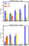 |
Fig. 9 Fraction of outflow force in each velocity regime for blueshifted (top) and redshifted (bottom) sides of outflow for all sources. Approximate errors of 10% are shown, resulting from uncertainty in the borders between the velocity regimes. |
4 Discussion
4.1 Jet and wind kinematics – the driving force of outflows
The exact origin of the large-scale outflows from protostars is still unclear. It is suggested that the narrow, highly-collimated jet from the protostar or the inner disk could power the entirety of the outflow (Raga & Cabrit 1993). However, models with jet bow-shocks that power the slow outflow fail to reproduce all of the observed kinematic features of the slow gas (Lee et al. 2002). Resolving the kinematic structure of the EHV bullets suggests, however, that a significant fraction of the momentum of the jet is ejected sideways, impacting the surrounding envelope (Santiago-García et al. 2009; Tafalla et al. 2017).
Directly studying the relationship between the outflow and jet is difficult, since the atomic and ionized jet is invisible in the same wavelength regime as the colder molecular outflows. Thus, studying protostars in their earliest stages of formation, when the jet is still mostly molecular, gives a unique opportunity to study the relation between the outflow and the jet. Our ALMA observations allow us to study three remarkable outflows with EHV jet components within one cloud. Moreover, it is often difficult to study outflows at high resolution since they propagate to vast distances very rapidly. Only a few of them have been studied to their full extent with ALMA (e.g., Arce et al. 2013). While it appears that the SMM1-a,b, and S68N outflows have indeed already propagated to tens of thousands of au (Dionatos et al. 2010; Yıldız et al. 2015), it is plausible that Ser-emb 8 (N) outflow is not as apparent from the observations with a larger field of view (Dionatos et al. 2010; Hull et al. 2014). This source thus provides an opportunity to study the full extent of the outflow.
The relation between the different components here is quantified by measuring the outflow force in three velocity components: slow and fast wing, and in the EHV jet. From Fig. 9 it is apparent that only for the blueshifted jet of Ser-emb 8 (N) is the EHV contribution (45%) to the total outflow force higher than that of the slow and fast wing components. The contribution of the EHV components to the outflow force in the other two sources is smaller than the contribution from the wing. Based on these findings, it seems that the force contained in the jet is generally not enough to power the total observed outflowing gas.
One of the explanations for the missing force is that the jet becomes atomic as the source evolves. Thus, measurements of the molecular component alone can underestimate the total mass of the gas. Such a scenario is supported by the observations of atomic oxygen from Herschel (van Kempen et al. 2010; Nisini et al. 2015). For a small sample of protostars, Nisini et al. (2015) show that the atomic jet becomes an important dynamical agent in more evolved sources (late Class 0/ Class I), while younger outflows have a significant fraction of the jet in the form of molecular gas. Typical mass-loss rates in the jet derived from atomic oxygen for the Class 0 sources targeted by Nisini et al. (2015) are between 1 and 10 × 10−7 M⊙ yr−1 whereas for the one Class I source HH46 they find 2–8 × 10⁻⁶ M⊙ yr−1, which showsthat the atomic jet becomes more important at the later stages of protostellar evolution.
The mass-loss rates of the molecular jets presented here are 7.0, 3.9, and 15.0 × 10⁻⁷ M⊙ yr−1 for Ser-emb 8 (N), SMM1-a, and SMM1-b, respectively. The atomic jet of SMM1-a has been probed in [O I] (Mottram et al. 2017)and [Fe II] (Dionatos et al. 2014). From these tracers, both authors find a consistent mass flux of 2–4 × 10⁻⁷ M⊙ yr−1, which is smaller than our molecular value by a factor of two. The total mass-loss of the slow and fast wing combined for SMM1-a is 1.4 × 10⁻⁵ M⊙ yr−1. While these results are consistent with the SMM1-a jet that is mostly molecular, as is expected for a young Class 0 source, it appears that the jet cannot be solely responsible for driving the outflow, even when the atomic component is taken into account.
Another explanation for the missing force in the molecular jet could be that the excitation temperature of the gas in the jet has been underestimated. Observations of high-J CO and SiO suggest that excitation conditions change at higher velocities, with density and gas temperature rapidly rising (Nisini et al. 2007; Lefloch et al. 2015; Kristensen et al. 2017). The assumed temperature here is 75 K, which is reasonable for a slow wing (Yıldız et al. 2015; van Kempen et al. 2016). However, if the jet has different excitation conditions with higher temperatures, the CO mass of the gas is underestimated. To test this possibility, we compare the change in relative contribution to the total outflow force for two other sets of temperatures. In one example we increased the temperature of the fast wing to 250 K, and the EHV temperature to 300 K – this is the temperature of the warm component identified with PACS observations (Karska et al. 2013, 2018; Kristensen et al. 2017; Dionatos et al. 2013). In the second case we used 250 K for the fast wing again, and increased the temperature of the EHV component to 700 K, which was fit as the temperature of the hot component in PACS. In Fig. 10 results of this comparison are presented for three cases for SMM1-a. The fraction of the EHV contribution to the total outflow force increases from 3 to 10%. A significant increase is seen in the fast wing with a change from 44 to 62%. For the case of SMM1-a, it does not change the general picture of the EHV jet that contributes only a small fraction of the outflow force.
Figure 11 shows how the outflow force contributions change for all of the sources in the redshifted outflow if the temperature is changed to 75, 250, and 700 K, for the slow wing, the fast wing, and the EHV jet, respectively. The SMM1-b EHV jet now contributes the majority of the outflow force, while for Ser-emb 8 (N), the fast wing becomes the primary component. This indicates that if the temperature of the gas in the jet is higher than assumed for the slow wing (75 K), the total mass of the gas and hence other properties derived from it can be significantly higher.
Nonetheless, the example of Ser-emb 8 (N) shows that young outflows that have not propagated to larger distances yet and, therefore, have a smaller number of shocks along the jet, can have a significant fraction of the outflow force in the EHV gas. Likely, oldersources like SMM1-a that are more affected by precession have a more complicated jet-outflow relation and thus the interpretation is less straightforward.
While the SMM1-d outflow also lacks EHV emission, the contribution of the fast wing to the total outflow force is substantial (~40%). Other characteristics of this source – for example, its bullet-like structure and lack of the well-defined cavity walls in CO – suggest a peculiar nature of the outflow, and thus its lack of EHV emission cannot be attributed to the more evolved nature of the outflow.
For both SMM1-d and S68N, there is potentially another reason why the EHV component is not detected: inclination. While for S68N we do not see a clear bullet-like structure, for SMM1-d it might well be that the bullets are seen moving at very high velocities, but in the plane of the sky. This is consistent with the fact that we see a significant blueshifted component on the redshifted side of the flow, which is consistent with the sideways expansion.
We can see an evolution of the outflow force distribution among the different velocity components, which cannot only be attributed to the chemical changes in the jet. One way to explain this is that a significant amount of outflow force is deposited in the fast and the slow wind very early in the protostellar evolution. Additional launching mechanisms like a wide-angle wind could also contribute to the bulk force released from the protostellar system.
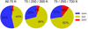 |
Fig. 10 Fraction of outflow force in three different components (slow, fast, EHV) of redshifted SMM1-a outflow for three different CO excitation temperatures used to calculate outflow force. On the left plot all of the components have 75 K; in the middle plot, slow wing has 75 K, fast wing has 250 K, and EHV jet has 300 K; on the right plot, slow wing has 75 K, fast winghas 250 K, and EHV jet has 700 K. The slow wing is yellow. |
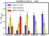 |
Fig. 11 Fraction of outflow force in each velocity regime, for redshifted side of outflow for all sources. Approximate errors of 10% are shown, resulting from uncertainty in the borders between the velocity regimes. The excitation temperatures used to calculate the outflow force are: 75 K for the slow wing, 250 K for the fast wing, and 700 K for the EHV jet. |
4.2 Relations with temperature and velocity components from HIFI
Understanding the far-infrared (FIR) emission from outflows is crucial to quantify and describe cooling processes around young protostars, as the majority of cooling occurs in this regime (Ceccarelli et al. 1996; Karska et al. 2013, 2018). The Herschel Space Observatory provides new insights into the kinematics via FIR line profiles from the HIFI instrument (e.g., Tafalla et al. 2013; Kristensen et al. 2013; Mottram et al. 2014).
Specifically, observations with HIFI of large numbers of low-mass protostars have shown that the high-J CO line profiles of shocked, outflowing gas can be decomposed universally into two velocity components. Subsequent radiative transfer modeling has linked these velocity components to the physical components of the protostellar system (Kristensen et al. 2017). Unfortunately, the spatial information from Herschel is limited, and single-dish low-J CO data show a different distribution from that of the high-J lines, as the low-J CO observations are sensitive to more extended emission (Santangelo et al. 2012; Tafalla et al. 2013). ALMA data are sensitive to small scale emission, and thus offer the opportunity to relate the spatially unresolved components of the HIFI emission (estimated to arise on a few hundred au scales, Mottram et al. 2014) with ALMA observations of low-J lines, allowing us to unveil the physical origin of the emission observed with HIFI.
Here we compare the ALMA observations of CO 2−1 toward Serpens SMM1 with Herschel/HIFI observations including CO 16−15, CO 10−9, and several water transitions (Yıldız et al. 2013; Kristensen et al. 2012, 2013; Mottram et al. 2014). Interferometric observations resolve the SMM1 system into at least five protostars with three active outflows; this can help to disentangle the various components of the system blended into one HIFI beam of typically 20′′. Figure A.1 shows three examples of comparisons between HIFI and ALMA spectral profiles.
There are some similarities between the HIFI velocity components for the SMM1 system and the ALMA low-J CO spectra. The offset HIFI component is seen in the SMM1-a spectra and is spatially linked to the ridge of the blueshifted emission of the SMM1-a outflow. The broad component appears similar to the fast wing CO 2−1 component and is present at both SMM1-a and SMM1-b outflows. The EHV bullet seen in water transitions from HIFI can be associated spatially with ALMA CO SMM1-b bullets, but it peaks at higher velocities than the SMM1-b jet. While it is impossible to spatially resolve the location of the water emission, this result suggests that water is formed in the higher velocity shock than CO or SiO. A detailed discussion of the comparison of ALMA observations with Herschel data is presented in the Appendix A.
4.3 The case of Ser-emb 8 (N): a pristine outflow-jet system
Many characteristics of Ser-emb 8 (N), such as its narrow opening angle of 25° and the high contribution of the molecular jet to the total force of the outflow, show that it is likely the youngest of the sources in the sample and therefore the best example of a pristine molecular jet and outflow system. It is also likely that we see most of the outflow within the ALMA field of view. This is in contrast to SMM1-a and b, which are known to extend to much larger scales (Davis et al. 1999; Dionatos et al. 2010). If so, the most distant bullet at 4500 au would have a dynamical age of only 350 yr for a velocity of 60 km s−1. In this section, we explore the spatial distribution of the analyzed velocity components of other molecules of the Ser-emb 8 (N) outflow. Figure 12 shows the spatial distribution of the fast and EHV velocity components for the CO, SiO, H2CO, and HCN.
One thing that is immediately apparent is the very similar shape of the SiO and HCN emission, which both form a redshifted bow-shock in the fast velocity component. On the blueshifted side, the shape of emission does not resemble a bow-shock, but both HCN and SiO appear mostly off the jet axis. The SiO and HCN bow-shock on the red side (Figs. 12d,e) surrounds one of the EHV bullets seen in CO (Fig. 12a). The weak blueshifted emission on the redshifted side of the outflow seen in SiO and HCN (velocities from –5 to –2 km s−1 with respectto the source velocity) is consistent with the sideways expansion of the gas due to interaction with the internal shock in the EHV bullet (Tafalla et al. 2017). This suggests a relation between EHV jets with the fast wing. Sideways ejections of the EHV gas can create slow shocks along the cavity walls. Herschel line profiles show that when the source exhibits EHV emission, the broad component is always present (Kristensen et al. 2012). The nearly identical shape of the SiO and HCN emission in the fast wing can be related to the same physical process that is responsible for the production of the SiO and HCN gas, as both species are enhanced in shocks (Schilke et al. 1997; Pineau des Forêts et al. 1990).
The most distant EHV bullet at 6000 au – corresponding to the dynamical age of 500 yr – is seen mostly in CO with SiO emission that is much fainter compared with the “younger” bullets. It is possible that grains have started to reform, causing the SiO depletion from the gas. The decrease in the SiO emission can, however, also be caused by the change in the excitation conditions along the jet: the density and the temperature of the gas likely decrease in the more distant bullets (Nisini et al. 2007).
H2CO is seen in only one bullet on the blueshifted side of Ser-emb 8 (N). This H2CO bullet is coincident with the CO peak of intensity along the jet at ~4000 au. Thus, the presence of H2CO can be related to the total density of the gas at that position – CO formation in the EHV jet is enhanced with density (Glassgold et al. 1991).
 |
Fig. 12 Schematic view of spatial distribution of different molecules and their relation with different velocity components in Ser-emb 8 (N) outflow. (a) In colorscale the CO moment 0 map is shown integrated over the EHV velocities, also overlaid on the following plots; (b) contours are SiO EHV emission captured at high spatial resolution, i.e., below 40 km s−1 ; (c) H2CO EHV emission (available only at low spatial resolution - synthesized beam is 1.′′65 × 1.′′13); (d) SiO fastwing emission; (e) HCN fast wing emission. The synthesized beams of continuum (black) and contour map (red) is shown in bottom-left corner. |
4.4 Chemistry of the velocity components
The first extensive chemical survey of the molecular jets revealed differences in the chemical composition of the slow and fast components and the EHV jet (Tafalla et al. 2010), the main conclusion being that the EHV component has more oxygen-containing molecules than the slow and the fast wing gas, which are carbon-rich (abbreviated as a higher C/O ratio). The high-resolution interferometric observations presented here are consistent with these single-dish studies: SiO abundances are enhanced with velocities up to those of the EHV jet for Ser-emb 8 (N) and redshifted SMM1-b. H2CO appears in one EHV bullet of Ser-emb 8(N). The HCN is present in the slow and the fast wing, but it does not appear in the EHV jet. Unique to our analysis is the ability to not only study the spectra but also relate the abundances with different spatial and velocitycomponents of the outflow.
The spatial distribution of molecules can indeed provide essential clues about the relation between different velocity components. The bow-shock structure in the redshifted part of the Ser-emb 8(N) outflow (fast wing, Fig. 12) is co-spatial with a gas bullet moving at much higher velocities. The interaction between the EHV jet and the ambient gas, and the origin of thechemical composition of the fast wing component and the jet, is described in Fig. 13. If the jet indeed has a low C/O ratio (Tafalla et al. 2010), the production of oxygen-bearing molecules takes place in the internal working surface of the jet. Then, the (sideways) expanding internal shock interacts with the surrounding ambient material (with a higher C/O ratio) where the production of other species, such as HCN, can take place.
Our results can also be compared with interferometric studies of the prototypical chemically rich outflow L1157 (e.g., Gueth et al. 1996; Arce et al. 2008; Codella et al. 2009, 2017), which is also known to have a molecular jet (Podio et al. 2016). The L1157 data show a chemical evolution with time along the outflow, while the jet impacts current shocked gas.
4.4.1 SiO
SiO is enhanced consistently for Ser-emb 8 (N) from the slow to the fast wing and then to the EHV jet, where it peaks in abundance. The enhancement of SiO in supersonic gas is commonly explained by sputtering and grain destruction, and the subsequent formation of the SiO in the gas phase through reactions of Si with OH in the shocked gas (Schilke et al. 1997; Gusdorf et al. 2008a,b). If the high-velocity jet is ejected in an atomic state thus containing ample atomic Si, SiO molecules can also be efficiently formed in the internal shocks in the jet that triggers the density enhancement (Glassgold et al. 1991; Tafalla et al. 2010).
There are differences among the SiO velocity profiles of the various sources. Ser-emb 8 (N) and SMM1-b, the two sources with the EHV emission, show weak emission at low velocities, with SiO emission peaking at high velocities. Such offsets in the peak of the emission can be caused by shock enhancement of the SiO abundance,which is consistent with models described above. S68N and SMM1-d, on the other hand, have SiO profiles that peak close to the systemic velocity and then decrease with velocity.
Nisini et al. (2007) see a similar dichotomy with the profiles for two protostellar outflows: L1448-mm, the prototypical EHV source, and L1157-mm, a classic example of the chemically rich outflow, with EHV bullets detected by Tafalla et al. (2015) and Podio et al. (2016). These authors attribute this difference to the temporal evolution of the outflow, where young shocks show offset peak profiles, while wing profiles peaking at low velocities correspond to the gas after the passage of a shock, where gas slowed down but retained its enhanced SiO abundance (Jiménez-Serra et al. 2009). It is possible that this temporal evolution can be observed within one outflow. The SiO abundance along the Ser-emb 8 (N) outflow decreases with the distance from the source for the EHV jet. On the other hand, the fast wing abundance increases with the distance from the source up to ~4000 au and then decreases toward the most distant CO bullet. This can be interpreted as the SiO being produced in the EHV gas and then consistently slowing down as the shell of the internal shock is expanding.
The similarity of the HCN and SiO emission in the bow shock of the Ser-emb 8(N) poses a challenge to this scheme. Their similar spatial and kinematic structure in the fast wing would suggest a similar origin; however, HCN is not seen in the EHV gas, and therefore its formation in the jet is unlikely. An alternative explanation for the SiO emission in the fast wing is a C−shock along the cavity walls. Figure 13 presents a schematic of this scenario. The formation of the SiO in the C−shocked gas is a process with a timescale of >100 yr (Gusdorf et al. 2008a), which would explain an enhancement at some distance from the protostar. If the EHV SiO emission arises from the production in the dense atomic jet gas (Glassgold et al. 1991), this process would occur much faster, explaining the high EHV SiO abundance close to the protostar (Hirano et al. 2010; Podio et al. 2016). The observed H2O line with HIFI, which appears faster than the EHV jet toward SMM1-b, can thus be interpreted as having been formed even earlier, that is, in the fastest component of the internal working surface of the jet.
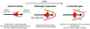 |
Fig. 13 Cartoon presenting interaction between molecular bullet and surrounding material. From the left to right a time evolution is shown starting with an internal shock within the molecular jet where atomic gas produces molecules inside a high-density internal working surface. As the bullet expands both forward and sideways it creates a shock with the surrounding ambient material; in the shocked gas, molecules are formed. The molecules observed in the EHV bullet are produced in lower C/O gas originating from the inner Mach disk, while the molecules from the shocked gas are formed from ambient gas with higher C/O ratio. |
4.4.2 H2CO
Tafalla et al. (2010) detected H2CO in EHV gas for the first time in only one source in their study of two EHV jets. In the case of L1448-mm, H2CO is also accompanied by CH3OH emission. In the slow wing, the H2CO abundance swiftly decreases with increasing velocity, which is likely to be easily destroyed in shocks, similar to CH3OH (Suutarinen et al. 2014). It is then remarkable that we see the H2CO in the high-velocity bullet of Ser-emb 8(N) (see Fig. 12c). More recently, several transitions of H2CO have been detected in the high-velocity component of the IRAS 2A outflow, while CH3OH has only been seen at low velocities (Santangelo et al. 2015). Figure 14 compares CO and H2CO spectra integrated toward the H2CO bullet for Ser-emb 8 (N).
Surprisingly, H2CO is seen in only one particular EHV bullet in the blueshifed jet of Ser-emb 8 (N). It is located at the peak of CO EHV emission but ahead of the SiO peak emission. The presence of the EHV H2CO emission for one of the three sources, and exclusively on one side of the emission, is puzzling. Two main explanations can be considered. One is the hydrogenation of CO on the reformed post-shock grains and then the subsequent release from the grains (e.g., Watanabe et al. 2004; Chuang et al. 2016). Within the bandwidth of the ALMA observations, many complex organic molecules are detected toward the protostars SMM1-a and S68N, with their location indicating an origin in the warm inner envelopes of the protostars (Tychoniec et al. 2018). Those molecules are not detected toward the position of the H2CO EHV bullet. If the release from the ices were a mechanism that is responsible for the H2CO emission at high velocities, one would expect the presence of other ice mantle components in the gas-phase. This is not seen in the case of this high-velocity bullet. Releasing H2CO from the ices is usually associated with lower outflow velocities; toward the L1157 outflow, H2CO is present in the shell of low-to-intermediate velocity gas. It is argued that the release of H2CO from the ices can trigger formation of the complex organic molecules in the gas-phase (Codella et al. 2017). Again, this is not seen here.
An alternative explanation for the H2CO emission in the high-velocity jet is gas-phase formation, mainly through the CH3 + O reaction (Dalgarno et al. 1973; Millar & Williams 1975) with CH3 abundance enhanced due to the high temperature. In particular, the C + H2 → CH + H reaction has a barrier of ~12 000 K, with subsequent reactions of CH and CH2 with H2 leading to CH3 having only somewhat smaller barriers (Agúndez et al. 2008; Bast et al. 2013). In this case, the abundance of the H2CO increases from the slow wing to the EHV component by at least a factor of two; therefore, the mechanisms responsible for the production and excitation of H2CO can be more efficient at higher velocities where temperatures are higher. A high abundance of atomic oxygen in the jet can further facilitate the reaction. This scenario would require the presence of some free atomic C in the jet, which would form H2CO but not HCN before all of the carbon is locked up in CO.
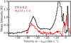 |
Fig. 14 Spectra of CO (black) and H2CO (red) of Ser-emb 8 (N) integrated on region where H2CO high-velocity emission is present. |
4.4.3 HCN
HCN traces the most energetic outflows associated with young, Class 0 sources (Jørgensen et al. 2004; Walker-Smith et al. 2014). High temperatures and densities of the shocked gas are responsible for HCN production. The enhancement of the HCN emission in shocks arises due to the H2 + CN → HCN + H reaction (Bruderer et al. 2009; Visser et al. 2018), which has an activation barrier of 960 K (Baulch et al. 2005). Both models and observations suggest that orders of magnitude increase in HCN abundance for gas temperatures above 200 K (Boonman et al. 2001; Lahuis et al. 2007).
We see HCN present in the slow and the fast wing, but it is depleted in the EHV jet. However, it appears that the presence of the fast HCN and SiO strongly depends on the presence of the EHV jet, as both HCN and SiO are observed in the bow shock in which the EHV bullet is embedded. It appears that, as an EHV bullet is present and as it ejects gas sideways at locations where it can interact with the cavity wall, both HCN and SiO are produced in these lower velocity C−type shocks. This interpretation is straightforward only for Ser-emb 8 (N); it is much harder to interpret the HCN in SMM1, as no HCN emission is observed toward SMM1-b and very little in SMM1-a. Tafalla et al. (2010) argue that HCN enhancement in the fast wing and depletion in the EHV jet is related to the atomic carbon abundance in the gas phase, specifically to a much lower C/O ratio in the EHV gas, which leads to the efficient formation of CO and SiO, but not HCN. It is unlikely that the gas in the EHV jet is colder than in the fast wing, so a temperature difference can not explain the lack of HCN in the EHV gas. Therefore our results support different chemical compositions of the EHV gas compared with the slow and the fast wings.
5 Summary
In this work, we use ALMA to study EHV molecular jets in the Serpens Main region. The relationship between the fast jet and slow outflowis studied, in an attempt to unveil the chemical composition of the different velocity components. The conclusions are as follows.
Out of five observed outflows, three show the EHV jet component. The high-sensitivity ALMA observations reveal that the EHV component in outflows from protostars is more frequent than previously thought.
The comparison of outflow forces between the slow outflow and EHV jet reveals that the observed force in the molecular jet is not sufficient to power the slow outflow in 3/5 sources. The most narrow and compact outflow (i.e., likely very young) in Ser-emb 8 (N) drives the jet with the highest EHV contribution of outflow force relative to the total energetic content of the flow. These results suggest an evolutionary sequence of the molecular emission from protostellar outflows where the EHV component is present in the youngest sources. The EHV and the fast wing components then subsequently disappear as the protostellar system evolves. Even after accounting for the atomic component, we conclude that the outflow force in the jet component is not sufficient to carry the entirety of the flow for all observed sources. This shows that a large fraction of the outflow force could already have been deposited inthe fast and the slow wind, or that another launching mechanism (i.e., a wide-angle wind) is also at play; however, the latter option cannot explain the bow-shock structures we observe in the fast wing component of Ser-emb 8(N).
The spatial distribution of the different molecular species is revealed in 0.′′4 ALMA observations; we focus in particular on the newly reported EHV jet from Ser-emb 8 (N). The fast wing SiO and HCN emission on the redshifted side of this outflow resembles bow-shocks that surround the EHV bullet, which indicates a relationship between the fast wing and the sideways ejections of the EHV jet.
The chemical composition of the velocity components of the outflow has been probed. The SiO abundance is enhanced from the slow to fast gas; the HCN is present from slow to fast wing but disappears in the EHV jet; and H2CO is only seen in the slow gas and in one EHV bullet exclusively in the blueshifted part of the Ser-emb 8 (N) jet. These results are in agreement with the single-dish results from Tafalla et al. (2010) where the EHV jet has a lower C/O ratio than the entrained slow and fast gas. Consistent velocity profiles of both molecules suggest that gas-phase formation is a plausible explanation for H2CO emission in the EHV jet. The HCN presence at the bow-shock (fast wing) is consistent with an increased temperature in the C−shocked region compared with the lower velocity gas. HCN depletion in the EHV gas can be associated with the lower C/O ratio in that gas.
The decrease in the SiO abundance in the EHV gas with distance from the protostar, combined with an increase in the fast wing, suggests that SiO produced in the EHV gas is slowed down, but remains abundant at lower velocities. The production of SiO and HCN in C-shocks (fast wing) after some time from the passage of the shock front, as expected by the models, provides an alternative explanation to an apparent temporal evolution of the abundances. We compare ALMA observations with the Herschel/HIFI velocity profiles of high-J CO and water, specifically by comparing the offset and broad components seen universally in the HIFI observations (Mottram et al. 2014; Kristensen et al. 2017) with the slow wing, the fast wing, and the EHV jets explored with ALMA CO 2−1 line profiles. The spatial location of the HIFI profiles is revealed; the fast wing has a similar profile to the HIFI broad component and EHV features are seen in both HIFI water emission and in ALMA spectra. However, the water EHV bullet peaks at higher velocities and is therefore formed first in the internal working surface of the jet.
Acknowledgements
The authors are grateful to the referee for comments that helped to improve the manuscript. Ł.T. would like to thank Benoît Tabone for stimulating discussions. This paper makes use of the following ALMA data: ADS/JAO.ALMA#2013.1.00726.S and ADS/JAO.ALMA#2016.1.00710.S. ALMA is a partnership of ESO (representing its member states), NSF (USA) and NINS (Japan), together with NRC (Canada), MOST and ASIAA (Taiwan), and KASI (Republic of Korea), in cooperation with the Republic of Chile. The Joint ALMA Observatory is operated by ESO, AUI/NRAO and NAOJ. Astrochemistry in Leiden is supported by the Netherlands Research School for Astronomy (NOVA), by a Royal Netherlands Academy of Arts and Sciences (KNAW) professor prize, and by the European Union A-ERC grant 291141 CHEMPLAN. The research of L.E.K. is supported by a research grant (19127) from VILLUM FONDEN. C.L.H.H. acknowledges the support of both the NAOJ Fellowship as well as JSPS KAKENHI grant 18K13586. This research made use of Astropy, a community-developed core Python package for Astronomy (Astropy Collaboration 2013, http://astropy.org); Matplotlib library (Hunter 2007); NASA’s Astrophysics Data System.
Appendix A Relations with temperature and velocity components from HIFI
The comparison of ALMA CO 2−1 observationswith HIFI high − J CO and H2O line profiles is presented in Fig. A.1. The HIFI CO 16−15 spectrum is plotted alongside three ALMA spectra in Fig. A.1a, one of which is averaged over the HIFI beam (13′′) for CO 16−15, and two of which are averaged over the region dedicated to SMM1-a and SMM1-b but limited to the borders of the HIFI beam. The HIFI spectra are shown with the Gaussian offset component overlaid based on the fit from Kristensen et al. (2013).
The offset component for SMM1 is seen in all water transitions targeted by Mottram et al. (2014), and in CO 16−15 (Kristensen et al. 2013). At the same time, CO 10−9 does not show a clear offset component (Yıldız et al. 2013). This suggests high temperatures in the offset component, and indeed the offset profile has been linked to the hot gas component (700 K) as seen in the rotational diagrams from PACS observations (Karska et al. 2013; Green et al. 2013; Kristensen et al. 2017). Radiative transfer modeling of the physical conditions for this component (Kristensen et al. 2013) suggests that this emission comes from a small emitting area (~100 AU; 0.′′25) with high densities (106 –107 cm−3).
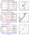 |
Fig. A.1 Comparison of CO 2−1 emission from SMM1 system with HIFI observations. Left: spectra from HIFI (blue), ALMA integrated with HIFI beam (black), ALMA spectra integrated with regions drawn to capture all emission from SMM1-a (purple) and SMM1-b (green) within HIFI beam. The velocity range from which the moment 0 map on the right was produced is indicated with the red shade. The Gaussian profiles for the relevant velocity components that were fit to the HIFI profiles for CO 16–15 (Kristensen et al. 2012) and H2O (Mottram et al. 2014) are shown. Right: moment 0 maps made by integrating the emission from range indicated by the red, shaded box on the left. Colors correspond to the spectra with SMM1-a outflow in green and SMM1-b outflow in purple. HIFI beam is plotted as a black circle. The beam size of the ALMA Band 6 spectral line (red) and continuum (black) is presented in the bottom-left corner of images. |
Hints about the spatial origin of the offset component can be seen with ALMA: the offset component is likely associated with the prominent blueshifted emission from SMM1-a close to the source (Fig. A.1a). This particular position has also been associated with a series of blueshifted water maser emissions (van Kempen et al. 2009)and a bright spot of ion emission in the near-IR (Dionatos et al. 2014). In Fig. A.1b, the H2O 111 − 000 spectrum isplotted with ALMA spectra: one is averaged over the HIFI beam (20′′) for H2O H2O 111 −000, and two are averaged over the region dedicated to SMM1-a and SMM1-b, but they are limited to the borders of the HIFI beam. The HIFI spectrum is shown with the broad Gaussian component that is overlaid based on the Mottram et al. (2014) fit. The redshifted broad component is seen mostly in the lower energy levels of water in the HIFI data (Mottram et al. 2014). It is explained by emission tracing warm (300 K) gas from the outflow cavity shocks, where the protostellar wind interacts with the outflow cavity walls (Kristensen et al. 2013; Mottram et al. 2014). It is also proposed that this component can trace the protostellar wind itself (Panoglou et al. 2012; Yvart et al. 2016). Figure A.1b shows that ALMA CO 2− 1 for SMM1-a and SMM1-b has a very similar line profile to the H2O 111−100 in the fast wing component. Spatially, the emission is widespread, coming from both sources.
It is worth noting that the broad component is much more prominent in the redshifted part of the HIFI spectra; similarly, the EHV jets are associated only with the redshifted jets for both SMM1-a and b. This shows that the presence of the jet could be linked to the presence of the broad component, and possibly part of the component arises as the high-velocity jet material ejected sideways interacts with the outflow cavity walls.
The broad component from the HIFI water emission seems coincident spectrally with the fast wing component in CO 2−1. The chemical signatures of the fast wing, such as abundance enhancement of the SiO and the presence of HCN, can then be linked to the outflow cavity shocks. In Fig. A.1c, the H2O 312−303 spectrum is plotted with ALMA spectra: one is averaged over the HIFI beam (20′′) for H2O 312−303, and two are averaged over the region dedicated to SMM1-a and SMM1-b, but they are limited to the borders of the HIFI beam. The EHV bullets seen prominently in CO 2−1 are not bright in the HIFI spectra. Although no EHV detection for this source with HIFI has been claimed, it seems that there is a faint emission in the two most energetic transitions observed by Mottram et al. (2014): 312 –303 and 312−221, which suggests that the water bullets might be associated with high temperatures, although due to higher frequency of the transitions and thus a smaller beam, less dilution can play a role at the same time. H2O (312 –303) shows a peak at 55 km s−1 while the 312 −221 shows a tentative detection at 72 km s−1.
At the same time CO 16–15 and 10–9 show no EHV emission, which suggests that the temperatures are not high enough to populate those levels. Even if the temperatures reach 700 K, the bullets are very compact and the filling factor is too small. Figure A.1c shows that H2O 312 –303 spectral EHV feature peaks outside the EHV peak for both SMM1-a and SMM1-b. The CO 2− 1 emission at the peak velocities of the water bullet shows that the emission could be associated with both jets. Spectra show that the water EHV feature peaks just as the SMM1-bCO 2−1 feature decreases. It is possible that the water feature is associated with the jet at higher temperatures, where CO 2−1 emission is weak.
Appendix B Additional figures
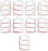 |
Fig. B.1 Spectra of CO in black, and different molecules as annotated in top-right corner in red. Spectra extracted from selected partof the outflow to highlight the key velocity components indicated in Figs. 2 and 3. Vertical dashed lines represent boundaries between different velocity regimes: slow wing, fast wing, and extremely high velocity. |
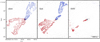 |
Fig. B.2 Integrated intensity maps of CO for different velocity regimes overlaid on Band 6 continuumin grayscale for SMM1-a. The emission is integrated over the velocities listed in Table 2. The synthesized beam of the CO (red) and continuum (black) is presented in bottom-left corner of EHV plot. The synthesized beam size of the continuum images is 0.′′35 × 0.′′33 and 0.′′55 × 0.′′45 for CO map. The contours are [3, 6, 9, 15, 20, 40] times the rms value. The rms values for each velocity channel, which are blueshifted and redshifted in K km s−1, are slow [18.8, 20.5], fast[5.8, 7.2], EHV [2.0, 2.8]. |
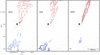 |
Fig. B.3 Same as Fig. B.2, but for SMM1-b. The rms values for each velocity channel, which are blueshifted and redshifted in K km s−1, are slow [17.5, 21.0], fast [5.3, 12.6], EHV [2.1, 3.7]. |
 |
Fig. B.4 Same as Fig. B.2, but for SMM1-d. The rms values for each velocity channel, which are redshifted in K km s−1 [20.7], [15.72]. No blueshifted and no EHV emission is detected toward this source. |
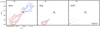 |
Fig. B.5 Same as Fig. B.2, but for S68N. The rms values for each velocity channel, which are blueshifted and redshifted in K km s−1, are slow [19.2, 13.8], fast [-, 4.7]. No EHV emission is detected toward this source. |
Appendix C Additional tables
Details of the observations used in this paper are listed in Table C.1 The calculated abundances of each molecule are shown in Tables C.2–C.6. For each molecule we calculated column density for the minimum and maximum expected Tex as listed in Table 3. We assume that values have 20% uncertainty, which arise from calibration, arbitrary defining velocity regimes, and other factors. Tables C.7–C.10 present the outflow forces that are notcorrected for inclination (see main text). Their absolute values are therefore uncertain by factors of a few.
Specifications of observations.
Column densities of targeted molecules per velocity regime for Ser-emb 8 (N).
Column densities of targeted molecules per velocity regime for S68N.
Column densities of targeted molecules per velocity regime for SMM1-a.
Column densities of targeted molecules per velocity regime for SMM1-b.
Column densities of targeted molecules per velocity regime for SMM1-d.
Outflow properties per velocity regime for Ser-emb 8 (N).
Outflow properties per velocity regime for S68N.
Outflow properties per velocity regime for SMM1-a.
Outflow properties per velocity regime for SMM1-b.
Outflow properties per velocity regime for SMM1-d.
References
- Agúndez, M., Cernicharo, J., & Goicoechea, J. R. 2008, A&A, 483, 831 [NASA ADS] [CrossRef] [EDP Sciences] [Google Scholar]
- André, P., Ward-Thompson, D., & Barsony, M. 1993, ApJ, 406, 122 [NASA ADS] [CrossRef] [Google Scholar]
- Arce, H. G., & Sargent, A. I. 2006, ApJ, 646, 1070 [NASA ADS] [CrossRef] [Google Scholar]
- Arce, H. G., Santiago-García, J., Jørgensen, J. K., Tafalla, M., & Bachiller, R. 2008, ApJ, 681, L21 [NASA ADS] [CrossRef] [Google Scholar]
- Arce, H. G., Mardones, D., Corder, S. A., et al. 2013, ApJ, 774, 39 [CrossRef] [Google Scholar]
- Astropy Collaboration (Robitaille, T. P., et al.) 2013, A&A, 558, A33 [NASA ADS] [CrossRef] [EDP Sciences] [Google Scholar]
- Bachiller, R. 1996, ARA&A, 34, 111 [NASA ADS] [CrossRef] [Google Scholar]
- Bachiller, R., Martin-Pintado, J., Tafalla, M., Cernicharo, J., & Lazareff, B. 1990, A&A, 231, 174 [NASA ADS] [Google Scholar]
- Bachiller, R., Terebey, S., Jarrett, T., et al. 1994, ApJ, 437, 296 [NASA ADS] [CrossRef] [Google Scholar]
- Bast, J. E., Lahuis, F., van Dishoeck, E. F., & Tielens, A. G. G. M. 2013, A&A, 551, A118 [NASA ADS] [CrossRef] [EDP Sciences] [Google Scholar]
- Baulch, D. L., Bowman, C. T., Cobos, C. J., et al. 2005, J. Phys. Chem. Ref. Data, 34, 757 [NASA ADS] [CrossRef] [Google Scholar]
- Boonman, A. M. S., Stark, R., van der Tak, F. F. S., et al. 2001, ApJ, 553, L63 [NASA ADS] [CrossRef] [Google Scholar]
- Bruderer, S., Benz, A. O., Bourke, T. L., & Doty, S. D. 2009, A&A, 503, L13 [NASA ADS] [CrossRef] [EDP Sciences] [Google Scholar]
- Cabrit, S., Codella, C., Gueth, F., & Gusdorf, A. 2012, A&A, 548, L2 [NASA ADS] [CrossRef] [EDP Sciences] [Google Scholar]
- Ceccarelli, C., Hollenbach, D. J., & Tielens, A. G. G. M. 1996, ApJ, 471, 400 [Google Scholar]
- Choi, M. 2009, ApJ, 705, 1730 [NASA ADS] [CrossRef] [Google Scholar]
- Chuang, K.-J., Fedoseev, G., Ioppolo, S., van Dishoeck, E. F., & Linnartz, H. 2016, MNRAS, 455, 1702 [Google Scholar]
- Codella, C., Benedettini, M., Beltrán, M. T., et al. 2009, A&A, 507, L25 [NASA ADS] [CrossRef] [EDP Sciences] [Google Scholar]
- Codella, C., Cabrit, S., Gueth, F., et al. 2014, A&A, 568, L5 [Google Scholar]
- Codella, C., Ceccarelli, C., Caselli, P., et al. 2017, A&A, 605, L3 [NASA ADS] [CrossRef] [EDP Sciences] [Google Scholar]
- Dalgarno, A., Oppenheimer, M., & Black, J. H. 1973, Nat. Phys. Sci., 245, 100 [NASA ADS] [CrossRef] [Google Scholar]
- Davis, C. J., Matthews, H. E., Ray, T. P., Dent, W. R. F., & Richer, J. S. 1999, MNRAS, 309, 141 [NASA ADS] [CrossRef] [Google Scholar]
- de Graauw, T., Helmich, F. P., Phillips, T. G., et al. 2010, A&A, 518, L6 [NASA ADS] [CrossRef] [EDP Sciences] [Google Scholar]
- Dionatos, O., Nisini, B., Codella, C., & Giannini, T. 2010, A&A, 523, A29 [NASA ADS] [CrossRef] [EDP Sciences] [Google Scholar]
- Dionatos, O., Jørgensen, J. K., Green, J. D., et al. 2013, A&A, 558, A88 [NASA ADS] [CrossRef] [EDP Sciences] [Google Scholar]
- Dionatos, O., Jørgensen, J. K., Teixeira, P. S., Güdel, M., & Bergin, E. 2014, A&A, 563, A28 [NASA ADS] [CrossRef] [EDP Sciences] [Google Scholar]
- Downes, T. P., & Cabrit, S. 2007, A&A, 471, 873 [NASA ADS] [CrossRef] [EDP Sciences] [Google Scholar]
- Dunham, M. M., Arce, H. G., Mardones, D., et al. 2014, ApJ, 783, 29 [NASA ADS] [CrossRef] [Google Scholar]
- Enoch, M. L., Evans, II, N. J., Sargent, A. I., & Glenn, J. 2009, ApJ, 692, 973 [NASA ADS] [CrossRef] [Google Scholar]
- Enoch, M. L., Lee, J.-E., Harvey, P., Dunham, M. M., & Schnee, S. 2010, ApJ, 722, L33 [Google Scholar]
- Frank, A., Ray, T. P., Cabrit, S., et al. 2014, in Protostars and Planets VI, eds. H. Beuther, R. S. Klessen, C. P. Dullemond, & T. Henning (Tucson, AZ: University of Arizona Press), 451 [Google Scholar]
- Frerking, M. A., Langer, W. D., & Wilson, R. W. 1982, ApJ, 262, 590 [NASA ADS] [CrossRef] [Google Scholar]
- Glassgold, A. E., Mamon, G. A., & Huggins, P. J. 1991, ApJ, 373, 254 [NASA ADS] [CrossRef] [Google Scholar]
- Green, J. D., Evans, II, N. J., Jørgensen, J. K., et al. 2013, ApJ, 770, 123 [NASA ADS] [CrossRef] [Google Scholar]
- Gueth, F., Guilloteau, S., & Bachiller, R. 1996, A&A, 307, 891 [NASA ADS] [Google Scholar]
- Guilloteau, S., Bachiller, R., Fuente, A., & Lucas, R. 1992, A&A, 265, L49 [NASA ADS] [Google Scholar]
- Gusdorf, A., Cabrit, S., Flower, D. R., & Pineau des Forêts, G. 2008a, A&A, 482, 809 [Google Scholar]
- Gusdorf, A., Pineau des Forêts, G., Cabrit, S., & Flower, D. R. 2008b, A&A, 490, 695 [NASA ADS] [CrossRef] [EDP Sciences] [Google Scholar]
- Hirano, N., Ho, P. P. T., Liu, S.-Y., et al. 2010, ApJ, 717, 58 [NASA ADS] [CrossRef] [Google Scholar]
- Hogerheijde, M. R., van Dishoeck, E. F., Salverda, J. M., & Blake, G. A. 1999, ApJ, 513, 350 [NASA ADS] [CrossRef] [PubMed] [Google Scholar]
- Hull, C. L. H., Plambeck, R. L., Kwon, W., et al. 2014, ApJS, 213, 13 [NASA ADS] [CrossRef] [Google Scholar]
- Hull, C. L. H., Girart, J. M., Kristensen, L. E., et al. 2016, ApJ, 823, L27 [NASA ADS] [CrossRef] [Google Scholar]
- Hull, C. L. H., Girart, J. M., Tychoniec, Ł., et al. 2017, ApJ, 847, 92 [NASA ADS] [CrossRef] [Google Scholar]
- Hunter, J. D. 2007, Comput. Sci. and Eng., 9, 90 [Google Scholar]
- Jansen, D. J. 1995, PhD Thesis, Leiden Observatory, Leiden University, RA Leiden, The Netherlands [Google Scholar]
- Jiménez-Serra, I., Martín-Pintado, J., Caselli, P., Viti, S., & Rodríguez-Franco, A. 2009, ApJ, 695, 149 [NASA ADS] [CrossRef] [Google Scholar]
- Jørgensen, J. K., Hogerheijde, M. R., Blake, G. A., et al. 2004, A&A, 415, 1021 [NASA ADS] [CrossRef] [EDP Sciences] [Google Scholar]
- Karska, A., Herczeg, G. J., van Dishoeck, E. F., et al. 2013, A&A, 552, A141 [NASA ADS] [CrossRef] [EDP Sciences] [Google Scholar]
- Karska, A., Kaufman, M. J., Kristensen, L. E., et al. 2018, ApJS, 235, 30 [NASA ADS] [CrossRef] [Google Scholar]
- Kauffmann, J., Bertoldi, F., Bourke, T. L., Evans, II, N. J., & Lee, C. W. 2008, A&A, 487, 993 [NASA ADS] [CrossRef] [EDP Sciences] [Google Scholar]
- Kristensen, L. E., van Dishoeck, E. F., van Kempen, T. A., et al. 2010, A&A, 516, A57 [NASA ADS] [CrossRef] [EDP Sciences] [Google Scholar]
- Kristensen, L. E., van Dishoeck, E. F., Bergin, E. A., et al. 2012, A&A, 542, A8 [NASA ADS] [CrossRef] [EDP Sciences] [Google Scholar]
- Kristensen, L. E., van Dishoeck, E. F., Benz, A. O., et al. 2013, A&A, 557, A23 [NASA ADS] [CrossRef] [EDP Sciences] [Google Scholar]
- Kristensen, L. E., van Dishoeck, E. F., Mottram, J. C., et al. 2017, A&A, 605, A93 [NASA ADS] [CrossRef] [EDP Sciences] [Google Scholar]
- Lahuis, F., Spoon, H. W. W., Tielens, A. G. G. M., et al. 2007, ApJ, 659, 296 [NASA ADS] [CrossRef] [Google Scholar]
- Lee, C.-F., Mundy, L. G., Stone, J. M., & Ostriker, E. C. 2002, ApJ, 576, 294 [NASA ADS] [CrossRef] [Google Scholar]
- Lee, C.-F., Ho, P. T. P., Bourke, T. L., et al. 2008, ApJ, 685, 1026 [NASA ADS] [CrossRef] [Google Scholar]
- Lefloch, B., Gusdorf, A., Codella, C., et al. 2015, A&A, 581, A4 [CrossRef] [EDP Sciences] [Google Scholar]
- Maury, A. J., André, P., Testi, L., et al. 2019, A&A, 621, A76 [NASA ADS] [CrossRef] [EDP Sciences] [Google Scholar]
- McMullin, J. P., Mundy, L. G., Wilking, B. A., Hezel, T., & Blake, G. A. 1994, ApJ, 424, 222 [NASA ADS] [CrossRef] [Google Scholar]
- McMullin, J. P., Mundy, L. G., Blake, G. A., et al. 2000, ApJ, 536, 845 [NASA ADS] [CrossRef] [Google Scholar]
- McMullin, J. P., Waters, B., Schiebel, D., Young, W., & Golap, K. 2007, ASP Conf. Ser., 376, 127 [Google Scholar]
- Millar, T. J., & Williams, D. A. 1975, MNRAS, 170, 51P [NASA ADS] [CrossRef] [Google Scholar]
- Mottram, J. C., Kristensen, L. E., van Dishoeck, E. F., et al. 2014, A&A, 572, A21 [NASA ADS] [CrossRef] [EDP Sciences] [Google Scholar]
- Mottram, J. C., van Dishoeck, E. F., Kristensen, L. E., et al. 2017, A&A, 600, A99 [NASA ADS] [CrossRef] [EDP Sciences] [Google Scholar]
- Nisini, B., Codella, C., Giannini, T., et al. 2007, A&A, 462, 163 [NASA ADS] [CrossRef] [EDP Sciences] [Google Scholar]
- Nisini, B., Santangelo, G., Giannini, T., et al. 2015, ApJ, 801, 121 [NASA ADS] [CrossRef] [EDP Sciences] [Google Scholar]
- Ortiz-León, G. N., Loinard, L., Kounkel, M. A., et al. 2017, ApJ, 834, 141 [NASA ADS] [CrossRef] [Google Scholar]
- Panoglou, D., Cabrit, S., Pineau des Forêts, G., et al. 2012, A&A, 538, A2 [NASA ADS] [CrossRef] [EDP Sciences] [Google Scholar]
- Pilbratt, G. L., Riedinger, J. R., Passvogel, T., et al. 2010, A&A, 518, L1 [CrossRef] [EDP Sciences] [Google Scholar]
- Pineau des Forêts, G., Roueff, E., & Flower, D. R. 1990, MNRAS, 244, 668 [NASA ADS] [Google Scholar]
- Plunkett, A. L., Arce, H. G., Corder, S. A., et al. 2013, ApJ, 774, 22 [NASA ADS] [CrossRef] [Google Scholar]
- Podio, L., Codella, C., Gueth, F., et al. 2016, A&A, 593, L4 [NASA ADS] [CrossRef] [EDP Sciences] [Google Scholar]
- Raga, A., & Cabrit, S. 1993, A&A, 278, 267 [Google Scholar]
- Raga, A. C., Canto, J., Calvet, N., Rodriguez, L. F., & Torrelles, J. M. 1993, A&A, 276, 539 [NASA ADS] [Google Scholar]
- San José-García, I., Mottram, J. C., van Dishoeck, E. F., et al. 2016, A&A, 585, A103 [NASA ADS] [CrossRef] [EDP Sciences] [Google Scholar]
- Santangelo, G., Nisini, B., Giannini, T., et al. 2012, A&A, 538, A45 [NASA ADS] [CrossRef] [EDP Sciences] [Google Scholar]
- Santangelo, G., Codella, C., Cabrit, S., et al. 2015, A&A, 584, A126 [NASA ADS] [CrossRef] [EDP Sciences] [Google Scholar]
- Santiago-García, J., Tafalla, M., Johnstone, D., & Bachiller, R. 2009, A&A, 495, 169 [NASA ADS] [CrossRef] [EDP Sciences] [Google Scholar]
- Schilke, P., Walmsley, C. M., Pineau des Forêts, G., & Flower, D. R. 1997, A&A, 321, 293 [NASA ADS] [Google Scholar]
- Suutarinen, A. N., Kristensen, L. E., Mottram, J. C., Fraser, H. J., & van Dishoeck, E. F. 2014, MNRAS, 440, 1844 [NASA ADS] [CrossRef] [Google Scholar]
- Tafalla, M., Santiago, J., Johnstone, D., & Bachiller, R. 2004, A&A, 423, L21 [NASA ADS] [CrossRef] [EDP Sciences] [Google Scholar]
- Tafalla, M., Santiago-García, J., Hacar, A., & Bachiller, R. 2010, A&A, 522, A91 [NASA ADS] [CrossRef] [EDP Sciences] [Google Scholar]
- Tafalla, M., Liseau, R., Nisini, B., et al. 2013, A&A, 551, A116 [NASA ADS] [CrossRef] [EDP Sciences] [Google Scholar]
- Tafalla, M., Bachiller, R., Lefloch, B., et al. 2015, A&A, 573, L2 [NASA ADS] [CrossRef] [EDP Sciences] [Google Scholar]
- Tafalla, M., Su, Y.-N., Shang, H., et al. 2017, A&A, 597, A119 [NASA ADS] [CrossRef] [EDP Sciences] [Google Scholar]
- Tychoniec, Ł., Hull, C. L. H., Tobin, J. J., & van Dishoeck, E. F. 2018, IAU Symp., 332, 249 [NASA ADS] [Google Scholar]
- van der Marel, N., Kristensen, L. E., Visser, R., et al. 2013, A&A, 556, A76 [NASA ADS] [CrossRef] [EDP Sciences] [Google Scholar]
- van der Tak, F. F. S., Black, J. H., Schöier, F. L., Jansen, D. J., & van Dishoeck, E. F. 2007, A&A, 468, 627 [NASA ADS] [CrossRef] [EDP Sciences] [Google Scholar]
- van Kempen, T. A., Wilner, D., & Gurwell, M. 2009, ApJ, 706, L22 [NASA ADS] [CrossRef] [Google Scholar]
- van Kempen, T. A., Kristensen, L. E., Herczeg, G. J., et al. 2010, A&A, 518, L121 [NASA ADS] [CrossRef] [EDP Sciences] [Google Scholar]
- van Kempen, T. A., Hogerheijde, M. R., van Dishoeck, E. F., et al. 2016, A&A, 587, A17 [NASA ADS] [CrossRef] [EDP Sciences] [Google Scholar]
- Visser, R., Bruderer, S., Cazzoletti, P., et al. 2018, A&A, 615, A75 [NASA ADS] [CrossRef] [EDP Sciences] [Google Scholar]
- Walker-Smith,S. L., Richer, J. S., Buckle, J. V., Hatchell, J., & Drabek-Maunder, E. 2014, MNRAS, 440, 3568 [NASA ADS] [CrossRef] [Google Scholar]
- Watanabe, N., Nagaoka, A., Shiraki, T., & Kouchi, A. 2004, ApJ, 616, 638 [NASA ADS] [CrossRef] [Google Scholar]
- Yıldız, U. A., Kristensen, L. E., van Dishoeck, E. F., et al. 2013, A&A, 556, A89 [NASA ADS] [CrossRef] [EDP Sciences] [Google Scholar]
- Yıldız, U. A., Kristensen, L. E., van Dishoeck, E. F., et al. 2015, A&A, 576, A109 [NASA ADS] [CrossRef] [EDP Sciences] [Google Scholar]
- Yvart, W., Cabrit, S., Pineau des Forêts, G., & Ferreira, J. 2016, A&A, 585, A74 [NASA ADS] [CrossRef] [EDP Sciences] [Google Scholar]
- Zhang, Y., Arce, H. G., Mardones, D., et al. 2016, ApJ, 832, 158 [NASA ADS] [CrossRef] [Google Scholar]
All Tables
All Figures
|
Fig. 1 Left: JCMT/SCUBA 850-μm map of Serpens Main region with numbers corresponding to SMM sources as classified by Davis et al. (1999). Contours are [3, 6, 12, 20, 40] × 0.50 mJy arcsec−2. Beam of the JCMT observations of 1.′′is indicated in the bottom-left corner. Right: ALMA 1.3 mm continuum of targeted protostars. For SMM9, field contours are [3, 6, 9, 12] × 0.53 mJy beam−1 and for SMM1 field contours are [3, 4, 5, 6, 9, 15, 40, 50] × 0.62 mJy beam−1. Synthesized beams of the ALMA observations are 0.′′35 × 0.′′33 for the SMM9 field and 0.′′36 × 0.′′30 for the SMM1 field. |
| In the text | |
|
Fig. 2 Integrated intensity maps of CO 2−1, SiO 5− 4, H2CO 303−202, and HCN 1−0 overlaid on the Band 6 (Band 3 for HCN) continuum in grayscale for Ser-emb 8 (N). The emission is integrated from the inner boundary of the slow wing component to the outer boundary of the EHV component as listed in Table 2 for the red and blueshifted emission. The exceptions are SiO and H2CO maps where only the channels obtained at high spatial resolution are plotted (<26 km s−1 for H2CO and <40 km s−1 for SiO). The synthesized beam size of the continuum images is 0.′′35 × 0.′′33 for Band 6 and 0.′′79 × 0.′′64 for Band 3; for spectral lines it is 0.′′53 × 0.′′45 (CO), 0.′′55 × 0.′′45 (SiO), 0.′′53 × 0.′′44 (H2CO), and 0.′′60 × 0.′′56 (HCN). The beam size of the Band 6 spectral line is presented in the bottom-left corner of the H2CO map and in HCN map for Band 3. Contour levels are [3, 6, 9, 15, 20, 40, 60, 80, 100] for CO, SiO, H2CO, and redshifted HCN, and [2, 3, 5, 6, 12] for blueshifted HCN, which were multiplied by rms value of moment 0 maps. The rms values for the blueshifted and redshifted side of the outflow in K km s−1 is as follows: CO [19.7, 14.4], SiO [2.2, 2.5], H2CO [2.8, 2.1], and HCN [9.3, 12.2]. Black ellipses indicate regions from which spectra were extracted for Figs. 4 and B.1. |
| In the text | |
|
Fig. 3 Similar to Fig. 2, but for remaining sources. S68N: contour levels are [3, 6, 9, 15, 20, 40, 60, 80, 100] for CO and HCN; [3, 8, 15, 30, 45] for SiO; and [3, 5, 9, 15, 20, 40] for H2CO, which were multiplied by the rms value of moment 0 maps. The rms values for the blueshifted and redshifted side of the outflow, in Kkm s−1: CO [19.5, 14.1], SiO [1.6, 1.9], H2CO [3.2, 2.0], and HCN [9.4, 12.7]. SMM1-a: contour levels are [3, 6, 9,15, 20, 40, 60, 80, 100] for all molecules, which were multiplied by the rms value of moment 0 maps. The rms values for the blueshifted and redshifted side of the outflow, in K km s−1 : CO [20.2, 20.6], SiO [3.6, 4.0], H2CO [2.0, 2.9], and HCN [7.5, 11.5]. SMM1-b: contour levels are [3, 6, 9, 15, 20, 40, 60, 80, 100] for CO, [3, 9, 36] for SiO, and [3, 5] for H2CO and HCN, which were multiplied by the rms value of moment 0 maps. The rms values for the blueshifted and redshifted side of the outflow, in K km s−1 : CO [18.7, 20.3], SiO [3.6, 4.0], H2CO [1.9, 2.9], and HCN [7.4, 11.5]. SMM1-d: only redshifted moment 0 map is presented as no blueshifted component has been detected toward this source. Contour levels are [3, 6, 9, 15, 20, 40, 60, 80, 100] for CO and HCN, [3, 12, 36] for SiO, and [2, 3] for H2CO, which were multiplied by the rms value of moment 0 maps. The rms values in K km s−1 are: CO [20.1], SiO [3.3], H2CO [2.7], and HCN [9.1]. Black ellipses indicate regions from which spectra were extracted for Fig. B.1. |
| In the text | |
|
Fig. 4 Spectra of CO (black) and SiO, H2CO, and HCN (red) for selected part of blueshifted part of Ser-emb 8 (N) outflow, indicated in Fig. 2. The dashed lines show boundaries between different velocity components. Full set of spectra for the other sources is shown in Fig. B.1. |
| In the text | |
|
Fig. 5 Integrated intensity maps of CO for different velocity regimes overlaid on Band 6 continuum in grayscale for Ser-emb 8 (N). The emission is integrated over the velocities listed in Table 2. The synthesized beams of the CO (red) and continuum (black) are showed in bottom-left corner of EHV plot with sizes 0.′′35 × 0.′′33 and 0.′′55 × 0.′′45 for continuum and CO, respectively. The contours are [3, 6, 9, 15, 20, 40, 60, 80, 100] times the rms value. The rms values for each velocity channel, which are blueshifted and redshifted in K km s−1, are slow [18.3, 13.7], fast [3.1, 4.5], EHV [1.7, 1.4]. |
| In the text | |
|
Fig. 6 Molecular abundances with respect to CO scaled by 104 for blueshifted (top) and redshifted (bottom) part of outflow for all sources. Gray triangles represent upper limits. Points on the plot show values calculated for the mean Tex of the range defined for each molecule, see Table 3. Error bars represent the column densities calculated for minimum and maximum values of the excitation temperature. To obtain the abundanceof the given molecule, the column density was divided by the CO column density (for Tex = 75 K.) measured in the region in which the emission from the molecule was above 3σ. The HCN emission is likely optically thick and therefore the abundance should be treated as a lower limit. |
| In the text | |
|
Fig. 7 Molecular abundances with respect to CO scaled by 104 for Ser-emb 8 (N). The distance from the protostar is on the x-axis. Panels from left to right are for the slow wing, the fast wing, and the EHV component. The abundances measured for three different regions along the outflow are shown for blueshifted and redshifted parts of the outflow separately. Abundances are measured in the same manner as in Fig. 6. The HCN emission is likely optically thick and therefore the abundance should be treated as a lower limit. |
| In the text | |
|
Fig. 8 Maps of SiO/CO ratio for blueshifted part of Ser-emb 8(N) outflow for each velocity component. For the EHV component, only the channels for which SiO emission was obtained at high spatial resolution are taken into account (<40 km s−1). The synthesized beams of the CO (red) and continuum (black) are shown in the bottom-left corner of EHV plot with sizes 0.′′35 × 0.′′33 and 0.′′55 × 0.′′45 for continuum and CO, respectively. The black contours show 1.3 mm continuum emission. |
| In the text | |
|
Fig. 9 Fraction of outflow force in each velocity regime for blueshifted (top) and redshifted (bottom) sides of outflow for all sources. Approximate errors of 10% are shown, resulting from uncertainty in the borders between the velocity regimes. |
| In the text | |
|
Fig. 10 Fraction of outflow force in three different components (slow, fast, EHV) of redshifted SMM1-a outflow for three different CO excitation temperatures used to calculate outflow force. On the left plot all of the components have 75 K; in the middle plot, slow wing has 75 K, fast wing has 250 K, and EHV jet has 300 K; on the right plot, slow wing has 75 K, fast winghas 250 K, and EHV jet has 700 K. The slow wing is yellow. |
| In the text | |
|
Fig. 11 Fraction of outflow force in each velocity regime, for redshifted side of outflow for all sources. Approximate errors of 10% are shown, resulting from uncertainty in the borders between the velocity regimes. The excitation temperatures used to calculate the outflow force are: 75 K for the slow wing, 250 K for the fast wing, and 700 K for the EHV jet. |
| In the text | |
|
Fig. 12 Schematic view of spatial distribution of different molecules and their relation with different velocity components in Ser-emb 8 (N) outflow. (a) In colorscale the CO moment 0 map is shown integrated over the EHV velocities, also overlaid on the following plots; (b) contours are SiO EHV emission captured at high spatial resolution, i.e., below 40 km s−1 ; (c) H2CO EHV emission (available only at low spatial resolution - synthesized beam is 1.′′65 × 1.′′13); (d) SiO fastwing emission; (e) HCN fast wing emission. The synthesized beams of continuum (black) and contour map (red) is shown in bottom-left corner. |
| In the text | |
|
Fig. 13 Cartoon presenting interaction between molecular bullet and surrounding material. From the left to right a time evolution is shown starting with an internal shock within the molecular jet where atomic gas produces molecules inside a high-density internal working surface. As the bullet expands both forward and sideways it creates a shock with the surrounding ambient material; in the shocked gas, molecules are formed. The molecules observed in the EHV bullet are produced in lower C/O gas originating from the inner Mach disk, while the molecules from the shocked gas are formed from ambient gas with higher C/O ratio. |
| In the text | |
|
Fig. 14 Spectra of CO (black) and H2CO (red) of Ser-emb 8 (N) integrated on region where H2CO high-velocity emission is present. |
| In the text | |
|
Fig. A.1 Comparison of CO 2−1 emission from SMM1 system with HIFI observations. Left: spectra from HIFI (blue), ALMA integrated with HIFI beam (black), ALMA spectra integrated with regions drawn to capture all emission from SMM1-a (purple) and SMM1-b (green) within HIFI beam. The velocity range from which the moment 0 map on the right was produced is indicated with the red shade. The Gaussian profiles for the relevant velocity components that were fit to the HIFI profiles for CO 16–15 (Kristensen et al. 2012) and H2O (Mottram et al. 2014) are shown. Right: moment 0 maps made by integrating the emission from range indicated by the red, shaded box on the left. Colors correspond to the spectra with SMM1-a outflow in green and SMM1-b outflow in purple. HIFI beam is plotted as a black circle. The beam size of the ALMA Band 6 spectral line (red) and continuum (black) is presented in the bottom-left corner of images. |
| In the text | |
|
Fig. B.1 Spectra of CO in black, and different molecules as annotated in top-right corner in red. Spectra extracted from selected partof the outflow to highlight the key velocity components indicated in Figs. 2 and 3. Vertical dashed lines represent boundaries between different velocity regimes: slow wing, fast wing, and extremely high velocity. |
| In the text | |
|
Fig. B.2 Integrated intensity maps of CO for different velocity regimes overlaid on Band 6 continuumin grayscale for SMM1-a. The emission is integrated over the velocities listed in Table 2. The synthesized beam of the CO (red) and continuum (black) is presented in bottom-left corner of EHV plot. The synthesized beam size of the continuum images is 0.′′35 × 0.′′33 and 0.′′55 × 0.′′45 for CO map. The contours are [3, 6, 9, 15, 20, 40] times the rms value. The rms values for each velocity channel, which are blueshifted and redshifted in K km s−1, are slow [18.8, 20.5], fast[5.8, 7.2], EHV [2.0, 2.8]. |
| In the text | |
|
Fig. B.3 Same as Fig. B.2, but for SMM1-b. The rms values for each velocity channel, which are blueshifted and redshifted in K km s−1, are slow [17.5, 21.0], fast [5.3, 12.6], EHV [2.1, 3.7]. |
| In the text | |
|
Fig. B.4 Same as Fig. B.2, but for SMM1-d. The rms values for each velocity channel, which are redshifted in K km s−1 [20.7], [15.72]. No blueshifted and no EHV emission is detected toward this source. |
| In the text | |
|
Fig. B.5 Same as Fig. B.2, but for S68N. The rms values for each velocity channel, which are blueshifted and redshifted in K km s−1, are slow [19.2, 13.8], fast [-, 4.7]. No EHV emission is detected toward this source. |
| In the text | |
Current usage metrics show cumulative count of Article Views (full-text article views including HTML views, PDF and ePub downloads, according to the available data) and Abstracts Views on Vision4Press platform.
Data correspond to usage on the plateform after 2015. The current usage metrics is available 48-96 hours after online publication and is updated daily on week days.
Initial download of the metrics may take a while.