| Issue |
A&A
Volume 626, June 2019
|
|
|---|---|---|
| Article Number | A109 | |
| Number of page(s) | 19 | |
| Section | Planets and planetary systems | |
| DOI | https://doi.org/10.1051/0004-6361/201935334 | |
| Published online | 20 June 2019 | |
Oscillatory migration of accreting protoplanets driven by a 3D distortion of the gas flow★
1
Institute of Astronomy, Charles University in Prague,
V Holešovičkách 2,
18000
Prague 8,
Czech Republic
e-mail: This email address is being protected from spambots. You need JavaScript enabled to view it.
2
Lund Observatory, Department of Astronomy and Theoretical Physics, Lund University,
Box 43,
22100
Lund,
Sweden
Received:
21
February
2019
Accepted:
27
April
2019
Abstract
Context. The dynamics of a low-mass protoplanet accreting solids is influenced by the heating torque, which was found to suppress inward migration in protoplanetary disks with constant opacities.
Aims. We investigate the differences in the heating torque between disks with constant and temperature-dependent opacities.
Methods. Interactions of a super-Earth-sized protoplanet with the gas disk are explored using 3D radiation hydrodynamic simulations.
Results. Accretion heating of the protoplanet creates a hot underdense region in the surrounding gas, leading to misalignment of the local density and pressure gradients. As a result, the 3D gas flow is perturbed and some of the streamlines form a retrograde spiral rising above the protoplanet. In the constant-opacity disk, the perturbed flow reaches a steady state and the underdense gas responsible for the heating torque remains distributed in accordance with previous studies. If the opacity is non-uniform, however, the differences in the disk structure can lead to more vigorous streamline distortion and eventually to a flow instability. The underdense gas develops a one-sided asymmetry which circulates around the protoplanet in a retrograde fashion. The heating torque thus strongly oscillates in time and does not on average counteract inward migration.
Conclusions. The torque variations make the radial drift of the protoplanet oscillatory, consisting of short intervals of alternating rapid inward and outward migration. We speculate that transitions between the positive and oscillatory heating torque may occur in specific disk regions susceptible to vertical convection, resulting in the convergent migration of multiple planetary embryos.
Key words: hydrodynamics / planets and satellites: formation / planet-disk interactions / protoplanetary disks
Movie attached to Fig. 6 is available at https://www.aanda.org
© ESO 2019
1 Introduction
Migration of protoplanets embedded in their natal gas disks is a key evolutionary step in the formation of each planetary system. Low-mass protoplanets, incapable of gap opening (Crida et al. 2006), undergo Type I migration under the influence of the gravitational torques exerted by the Lindblad spiral wakes (Goldreich & Tremaine 1979; Ward 1986) and by the gas in their corotation region (Ward 1991; Masset 2002; Tanaka et al. 2002; Paardekooper & Mellema 2006, 2008; Baruteau & Masset 2008; Masset & Casoli 2009; Paardekooper & Papaloizou 2009; Baruteau et al. 2011). Type I migration has a complicated relationship with disk structure and thermophysics (e.g. Kley & Crida 2008; Paardekooper et al. 2010, 2011; Lega et al. 2015). A detailed understanding of the underlying mechanism is therefore essential for the creation of realistic population synthesis models (e.g. Coleman & Nelson 2016).
A low-mass protoplanet evolving in a radiative disk has recently been shown to be subject to thermal torques (Lega et al. 2014; Benítez-Llambay et al. 2015; Masset & Velasco Romero 2017; Masset 2017) related to the thermal perturbations induced by the protoplanet in its vicinity. If the protoplanet itself is cold and non-luminous (Lega et al. 2014), the gas arriving in its potential well becomes heated, mostly as a result of compression (by means of the thermodynamic “PdV ” term). The resulting temperature excess becomes smoothed out by radiative transfer, so when the gas leaves the high-pressure region it lacks some of its internal energy – compared to the state before the compression – and therefore becomes colder and overdense. Two overdense lobes appear along the streamlines outflowing from the Hill sphere and their asymmetry makes the total torque acting on the protoplanet more negative, enhancing the inward migration. This process is known as the cold-finger effect (Lega et al. 2014).
In the opposite limit, the protoplanet is hot as a result of the solid material deposition during its formation (e.g. by pebble accretion; Ormel & Klahr 2010; Lambrechts & Johansen 2012). In such a case, the luminous protoplanet acts as a local heat source for the surrounding gas. Once the gas is heated, it becomes underdense compared to the situation without accretion heating. Benítez-Llambay et al. (2015) performed 3D radiation hydrodynamic simulations with the assumption of constant disk opacity and found that the hot protoplanet on a fixed circular orbit creates two underdense lobes of gas, again associated with the outflow from the Hill sphere. The rear lobe (positioned behind the protoplanet outwards from its orbit) is dominant, therefore there is an overabundance of gas ahead of the protoplanet and the resulting torque becomes more positive, supporting outward migration. The positive enhancement was named the heating torque. It was proposed to be an additional mechanism (along with other possibilities; see e.g. Rafikov 2002; Paardekooper & Mellema 2006; Morbidelli et al. 2008; Li et al. 2009; Yu et al. 2010; Kretke & Lin 2012; Bitsch et al. 2013; Fung & Chiang 2017; Brasser et al. 2018; Miranda & Lai 2018; McNally et al. 2019) capable of preventing the destruction of terrestrial-sized planetary embryos by an overly efficient inward migration (Korycansky & Pollack 1993; Ward 1997; Tanaka et al. 2002).
Moreover, the heating torque has important dynamical consequences for migrating protoplanets (Brož et al. 2018; Chrenko et al. 2018) because it can excite orbital eccentricities and inclinations by means of the hot-trail effect (Eklund & Masset 2017; Chrenko et al. 2017), which counteracts the otherwise efficient eccentricity and inclination damping by waves (Tanaka & Ward 2004; Cresswell et al. 2007).
Nevertheless, the heating torque has not been extensively studied in 3D radiative disks with non-uniform opacities. However, realistic opacity functions (Bell & Lin 1994; Semenov et al. 2003; Zhu et al. 2012) are of great significance for the disk structure and planet migration (e.g. Kretke & Lin 2012; Bitsch et al. 2013) and this study shows that the heating torque is affected as well.
In this paper, we reinvestigate the thermal torques acting on a low-mass protoplanet, with special emphasis on the heating torque in a disk with non-uniform opacity. We examine the streamlines near the protoplanet and point out the importance of their 3D distortion for redistribution of the hot underdense gas responsible for the heating torque.
2 Model
We considera protoplanetary system consisting of a central protostar surrounded by a disk of coupled gas and dust in which a single protoplanet is embedded. The fluid part of the disk model accounts only for the gas, assuming the dust is a passive tracer that acts as the main contributor to the material opacity.
2.1 Governing equations
The disk is described using Eulerian hydrodynamics on a staggered spherical mesh centred on the protostar. The spherical coordinates consist of the radial distance r, azimuthal angle θ, and colatitude ϕ. Our model is built on top of the hydrodynamic module of FARGO3D1 (Benítez-Llambay & Masset 2016), which solves the equations of continuity and momentum of a fluid
 (1)
(1)
![Mathematical equation: \begin{equation*} \frac{\partial\vec{v}}{\partial t} + \left(\vec{v}\cdot\nabla\right){\vec{v}} = - \frac{\nabla P}{\rho} - \nabla\Phi + \frac{\nabla\cdot\tens{T}}{\rho} - \left[2\vec{\Omega}\times\vec{v}+\vec{\Omega}\times\left(\vec{\Omega}\times\vec{r}\right) \right],\end{equation*}](/articles/aa/full_html/2019/06/aa35334-19/aa35334-19-eq2.png) (2)
(2)
where ρ is the volume density, t is time, v is the flow velocity vector (with the radial, azimuthal, and vertical components vr, vθ and vϕ), P is pressure, Φ is the gravitational potential of the protostar and the protoplanet, T is the viscous stress tensor (Benítez-Llambay & Masset 2016), r is the radius vector and Ω is the angular velocity vector, which is non-zero because we work in the reference frame corotating with the protoplanet.
To account for the energy production, dissipation and transport in the disk, we implement the two-temperature energy equations for the gas and the radiation field according to the formulation of Bitsch et al. (2013):
![Mathematical equation: \begin{equation*} \frac{\partial E_{\mathrm{R}}}{\partial t} + \nabla\cdot\vec{F} = \rho\kappa_{\mathrm{P}}\left[4\sigma T^{4} - cE_{\mathrm{R}} \right],\end{equation*}](/articles/aa/full_html/2019/06/aa35334-19/aa35334-19-eq3.png) (3)
(3)
![Mathematical equation: \begin{equation*} \frac{\partial \epsilon}{\partial t} + \left(\vec{v}\cdot\nabla\right)\epsilon = -P\nabla\cdot\vec{v} - \rho\kappa_{\mathrm{P}}\left[ 4\sigma T^{4} - cE_{\mathrm{R}} \right] + Q_{\mathrm{visc}} + Q_{\mathrm{art}} + Q_{\mathrm{acc}},\end{equation*}](/articles/aa/full_html/2019/06/aa35334-19/aa35334-19-eq4.png) (4)
(4)
where ER is the radiative energy, F the radiation flux, κP the Planck opacity, σ the Stefan–Boltzmann constant, T the gas temperature, c the speed of light, ɛ the internal energy of the gas, and Qvisc the viscous heating term (Mihalas & Weibel Mihalas 1984). Furthermore, Qart describes the heating due to the artificial viscosity (Stone & Norman 1992), and Qacc the heat released when the protoplanet is accreting. Stellar irradiation is neglected in this paper for simplicity although our code is capable of including it as well.
The state equation of the ideal gas is used:
 (5)
(5)
where γ is the adiabatic index and cV is the specific heat at constant volume, which can be expressed as cV = R∕(μ(γ − 1)), where R is the universal gas constantand μ is the mean molecular weight.
The flux-limited diffusion approximation (FLD; Levermore & Pomraning 1981) is adopted to obtain a closure relation for the radiation flux,
 (6)
(6)
where κR is the Rosseland opacity and λlim is the flux limiter of Kley (1989). For the opacities, we assume that the Planck and Rosseland means are similar enough to be replaced with a single value κ. This is a valid assumption in the cold regions of protoplanetary disks that we aim to study (Bitsch et al. 2013). The detailed opacity law will be specified later in Sect. 2.3.
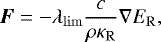
The accretion luminosity of the protoplanet is given by
 (7)
(7)
where G is the gravitational constant, Mp is the mass of the protoplanet, Ṁp is its accretion rate, and Rp is the radius of the protoplanet. In writing the second equality, we introduce the mass doubling time τ = Mp∕Ṁp, which is a free parameter that controls the accretion rate in our model (see Sect. 2.2).
We assume that the radiation flux from the protoplanet is completely absorbed by the optically thick gas in the eight grid cells enclosing the protoplanet (Benítez-Llambay et al. 2015; Eklund & Masset 2017; Lambrechts & Lega 2017). The accretion heating, which is non-zero only within these cells, is then simply
 (8)
(8)
where V is the total volume of the heated cells.
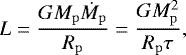
The disk evolves in the combined gravitational potential of the central protostar and the embedded protoplanet:
 (9)
(9)
where M⋆ is the mass of the protostar and d is the cell-protoplanet distance. The planetary potential is smoothed to avoid numerical divergence at the protoplanet location (d = 0) using the tapering cubic-spline function fsm of Klahr & Kley (2006):
![Mathematical equation: \begin{equation*} f_{\mathrm{sm}} = \left\{\begin{array}{@{}ll} 1, &\displaystyle \left(d > r_{\mathrm{sm}} \right),\\ \left[\left( \displaystyle\frac{d}{r_{\mathrm{sm}}} \right)^{4} -2\left( \displaystyle\frac{d}{r_{\mathrm{sm}}} \right)^{3} + 2\displaystyle\frac{d}{r_{\mathrm{sm}}} \right], &\displaystyle \left(d \leq r_{\mathrm{sm}} \right), \end{array}\right.\end{equation*}](/articles/aa/full_html/2019/06/aa35334-19/aa35334-19-eq10.png) (10)
(10)
where the smoothing length rsm is a fraction of the Hill sphere radius of the protoplanet (see Sect. 2.2). Orbital evolution of the protoplanet is tracked using the IAS15 integrator (Rein & Spiegel 2015) from the REBOUND2 package (Rein & Liu 2012), which we interfaced with FARGO3D.
Although FARGO3D is an explicit hydrodynamic solver, implementing Eqs. (3) and (4) in an explicit form would lead to a very restrictive Courant condition on the largest permitted time step length. To avoid such a time step limitation, it is advantageous to solve the energy equations in an implicit form. We thus follow the discretisation and linearisation proposed by Bitsch et al. (2013), with a minor modification introduced in Appendix A.
The solution of the implicit problem is obtained iteratively by minimizing the residual r ≡ Ax −b, where A is the matrix of the linear system, x is the solution vector, and b is the right-hand side vector. Our iterative solver uses the improved bi-conjugate stabilised method (IBiCGStab; Yang & Brent 2002) with the Jacobi preconditioning. The convergence criterion is ∥r ∥∕∥b∥ < 10−4, where the norms are calculated in the L2 space.
2.2 Initial conditions and parameters
Initial conditions describing the disk are adopted from Kley et al. (2009) and Lega et al. (2014). The surface density follows the power-law function Σ = 484(r/(1 au))−0.5 g cm−2. The initial Σ is converted into the initial ρ assuming the disk is vertically isothermal. The velocity field is given by balancing the gravitational acceleration from the protostar, the acceleration due to the pressure gradient, and the centrifugal acceleration. We assign constant kinematic viscosity ν = 1015 cm2 s−1 to the gas to mimic the angular momentum transport in the disk driven by physical effects outside the scope of this study (e.g. the turbulent eddy viscosity). The initial aspect ratio is h = H∕r = 0.05, where H is the pressure scale height. The disk is therefore initially non-flaring but we point our that h evolves during the simulations. The adiabatic index is γ = 1.43 and the mean molecular weight is μ = 2.3 g mol−1, corresponding to the solar mixture of the hydrogen and helium.
We assume a single embedded super-Earth with the mass Mp = 3 M⊕, orbiting on a circular orbit at the heliocentric distance of Jupiter: ap ≡ aJ = 5.2 au. Unless otherwise specified, the orbit is held fixed in our simulations, i.e. the protoplanet is not allowed to migrate and the torque we measure is the static torque. The simulations are performed in the reference frame corotating with the protoplanet at the Keplerian angular frequency  and the smoothing length for the tapering function of the gravitational potential fsm is rsm = 0.5RH, where
  is the Hill sphere radius. We study both cases with and without planetary accretion, corresponding to the hot- and cold-protoplanet limit, respectively. In the simulations with the accretion, we assume the mass-doubling time τ = 100 kyr, which is a value within the range of the expected pebble accretion rates (Lambrechts & Johansen 2014; Chrenko et al. 2017). The resulting luminosity of the protoplanet is L ≃ 4.2 × 1027 erg s−1.
2.3 Opacities
Using the initial disk parameters, we setup two fiducial disk models that only differ in the material opacity function. The opacity is either constant or follows a slightly modified (see below) prescription of Bell & Lin (1994). To distinguish between the models, we use the abbreviations κconst-disk and κBL -disk, respectively. The exact value of the opacity in the κconst-disk is tuned to be the same as in the κBL-disk at the location of the protoplanet ap, leading to κconst ≡ κBL(r = ap) = 1.11 cm2 g−1.
The unmodified opacity from Bell & Lin (1994), which we denote  , is a fitting law that sets κ as a function of the local gas density and temperature. The table spans several regimes corresponding to the presence (or absence) of dust or molecular species dominant in protoplanetary disks. Using
  in our simulations with the accretion heating of the protoplanet could cause strong local opacity gradients, because we expect the temperature perturbations to reach ~ 101 K at distances of one cell size from the centre of the protoplanet.
In practice, we apply the opacity law of Bell & Lin in a simplified way, using  , where the bared quantities are azimuthally computed arithmetic means and the dependence on the θ-coordinate is therefore dropped. This helps us to distinguish the effects caused by the global structure of the disk from those related to the local κ-T-ρ feedback. To justify our approach, we verify in Appendix B that the unmodified opacity table
  of Bell & Lin (1994) does not change our conclusions.
The fiducial κconst- and κBL-disks are discussed throughout the majority of the paper, with the exception of Sect. 3.6 where we study the dependence of the heating torque on the opacity gradient within the disk.
2.4 Grid resolution and boundary conditions
Migration oflow-mass protoplanets critically depends on the grid resolution, we therefore combine the well-established disk extent and resolution from Lega et al. (2014; in the azimuthal and vertical direction) and Eklund & Masset (2017; in the radial direction). The disk radially stretches from rmin = 3.12 au to rmax = 7.28 au and is resolved by 512 rings. We prevent any vertical motions of the protoplanet in our simulations by assuming that the solution is symmetric with respect to the midplane. One of the disk boundaries in the colatitude is therefore located at the midplane (ϕ = π∕2); the vertical extent above the midplane is 7°. The colatitude is resolved by 64 zones. In the azimuth, we use only 1 sector in our preparatory simulations without the protoplanet and 1382 sectors in our simulations with the embedded protoplanet. The resulting local resolution is eight cells per RH in the r- and ϕ-directions and three cells per RH in the θ-direction (see also Appendix B.2 for a simple resolution test).
The azimuthal boundary conditions are periodic for all primitive quantities. The radial boundary conditions are symmetric for ρ, ɛ, and vϕ and reflecting for vr. ER is set to a zero gradient and vθ is extrapolated using the same radial dependence as for the Keplerian rotation velocity. The boundary conditions in colatitude are symmetric for ρ, ɛ, vr and vθ, and reflecting for vϕ. ER is symmetrised at the midplane boundary and set to  at the remaining boundary in the colatitude, where aR is the radiation constant and T0 ≡ 5 K is the ambient temperature that allows for vertical radiative cooling of the disk. Additionally, wave-damping conditions of de Val-Borro et al. (2006) are imposed near the radial edges and also near the disk surface.
3 Simulations
3.1 Equilibrium disks
Since we usea non-isothermal equation of state and we also account for the energy production and transfer, the parametric setup of the disk, which was discussed so far, is not stationary. Therefore, before the simulations with the embedded protoplanet are conducted, we let both disks (κconst-disk and κBL -disk) numerically evolve over a timescale of 100 Porb, where Porb = 2π∕ΩJ.
The equilibrium state after the relaxation is presented in Fig. 1. We plot the radial profiles of the midplane temperature T, opacity κ, entropy S = P∕ργ and aspect ratio h = H∕r, where the pressure scale height is determined as H = cs∕ΩK and the sound speed as  .
.
The constant opacity of the κconst-disk makes all the remaining radial dependences rather shallow. The aspect ratio is almost flat, only slightly increasing with the radial distance. In the κBL -disk, on the other hand, the opacity has a peak near 3.5 au, where the water ice evaporates for the given setup, and decreases at larger radii. Therefore, the efficiency of the disk cooling increases and simultaneously, the efficiency of the viscous heating diminishes with the dropping relative velocity of the shearing layers. Consequently, the aspect ratio radially decreases as the energy budget is not sufficient to puff up the disk. In such a disk, T and S profiles radially decrease more steeply compared to the κconst-disk.
3.2 Torque evolution
Starting from the relaxed state of the disks, we copy the hydrodynamic quantities in the azimuthal direction to expand the resolution from a single sector to the desired 1382 sectors. The protoplanet is inserted and we simulate 30 Porb of evolution while neglecting any accretion and accretion heating of the protoplanet. The aim of this part of the simulation is to allow the disk to adjust to the presence of a gravitational perturber and to acquire a converged value of the disk torque in the absence of the accretion heating, corresponding to the cold-protoplanet limit. For the κBL -disk, this part of the simulation is similar to the experiments in Lega et al. (2014). Subsequently, we continue the simulation for another 30 Porb during which we let the planetary mass grow while releasing the accretion heat into the gas disk according to Eqs. (7) and (8).
Figure 2 shows the temporal evolution of the torque exerted on the protoplanet by the κconst-disk and κBL -disk. During the phase without accretion heating, the torque converges to a stationary value during 10 Porb. The torque value in the κBL-disk is more positive compared tothe κconst-disk, which is because the steeper radial decline of the entropy in the κBL-disk enhances the positive entropy-driven part of the corotation torque (Paardekooper & Mellema 2006; Baruteau & Masset 2008).
When the accretion heating is activated in the κconst-disk, a positive contribution is added to the torque, in accordance with the results of Benítez-Llambay et al. (2015). The torque slightly oscillates at first, but the amplitude of the oscillations decreases in time and becomes negligible at t = 50 Porb.
On thecontrary, when the accretion heating is activated in the κBL -disk, the outcome of the heating torque becomes very different. Strong oscillations of the disk torque are excited almost immediately and they do not vanish in time; instead, their amplitude remains the same. The arithmetic mean of the torque measured in the time interval 30–60 Porb is 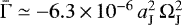 , implying that the torque is more negative compared to the situation without accretion heating (the mean torque in the interval 20–30 Porb is
 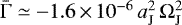 ). The amplitude of the variations with respect to the mean value is
 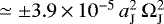 and the oscillation period is ≃ 2.1 Porb.
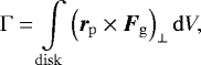
The torque oscillations are unexpected and we therefore focus throughout the rest of the paper on finding the physical mechanism that excites them. The occurrence of oscillations suggests that the gas distribution around the protoplanet is changing during the simulation, as we can demonstrate using the integral expression for the disk torque,
 (11)
(11)
where rp is the radius vector of the protoplanet, Fg is the gravitational force of a disk element, the vertical component of the cross product is considered, and we integrate over the disk volume. Only a non-zero azimuthal component of Fg can lead to a non-vanishing cross product in the integral, and therefore any oscillations of Γ must be related to a variation of Fg,θ. In other words, there must be an azimuthal asymmetry in the gas distribution with respect to the protoplanet for the torque to be non-zero and only a temporal redistribution of the asymmetry can cause a torque oscillation.
Our strategy throughout the remainder of Sect. 3 is the following: first, we focus on the κconst-disk simulation in Sect. 3.3. Although similar simulations were analysed by Benítez-Llambay et al. (2015), our aim is to focus on the 3D gas flow that has not yet been described. Our findings are then expanded for the κBL -disk simulation in Sect. 3.4 where we relate the gas redistribution to the oscillatory behaviour of the torque. Section 3.5 is devoted to identifying the key physical mechanisms that affect the gas flow. In Sect. 3.6, we vary the disk opacity gradient and study its impact on the torque oscillation. Finally, we relax the assumption of a fixed orbit and explore how the protoplanet migrates in Sect. 3.7.
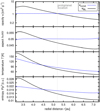 |
Fig. 1 Radial profiles of the characteristic quantities in the κconst-disk (dashed bluecurves) and the κBL-disk (solid black curves) after their numerical relaxation over t = 100 Porb. From top to bottom panels: opacity κ, aspect ratio h = H∕r, temperature T and entropy S = P∕ργ. Midplane values are displayed (or used to derive h). The dotted vertical line indicates the orbital distance of the protoplanet, ap = 5.2 au. |
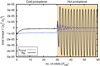 |
Fig. 2 Temporal evolution of the total torque exerted on the protoplanet (Mp = 3 M⊕) by the κconst-disk (dashed bluecurve) and the κBL-disk (solid black curve). For t ≤ 30 Porb, the protoplanet is not accreting. Its accretion and the respective heating are activated for t > 30 Porb, as also highlighted by a yellow background. While the blue curve evolves as expected, i.e. gains a positive boost when the accretion heating is initiated (Benítez-Llambay et al. 2015), the black curve does not converge and instead exhibits strong oscillations between positive and negative values. The red horizontal dotted line shows the mean value of the oscillating black curve and demonstrates that the heating torque makes the total torque more negative in this case. |
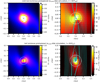 |
Fig. 3 Hydrodynamic quantities in the midplane of the κconst-disk close to the protoplanet. Top row: cold protoplanet right before the accretion heating is initiated (at t = 30 Porb). Bottom row: steady state of gas around the hot protoplanet (at t = 60 Porb). The figure isconstructed as a Cartesian projection of the spherical grid. The density maps (left) display the perturbation (ρ − ρ0)∕ρ0 relative to the equilibrium disk (t = 0 Porb), the temperature map for the cold protoplanet (top right) shows the absolute values, and the temperature map for the hot protoplanet (bottom right) shows the excess with respect to the cold protoplanet (by subtracting T(t = 30 Porb) from T(t = 60 Porb)). The position of the protoplanet is marked with the cross, the extent of its Hill sphere is bordered by the circle. The green curves (right) show the topology of streamlines in the frame corotating with the protoplanet. In the inertial frame, the protoplanet would orbit counterclockwise. The streamlines outwards from its orbit thus depict the flow directed from y > 0 to y < 0; the inward streamlines are oriented in the opposite direction. A detailed view of the streamlines is provided in Fig. 5 where we also sort them according to their type. |
3.3 Steady state of the heated gas
In this section, the κconst-disk simulation is analysed.
3.3.1 Midplane
Figure 3 compares the midplane density and temperature distribution around the cold and hot protoplanet. We display the state of the simulation at t = 30 (i.e. at the final stage of the phase without accretion heating) and 60 Porb (i.e. at the final stage of the phase with accretion heating). The latter represents the steady state of gas around the accreting protoplanet and we verified that such a distribution is achieved early (at t ≃ 31 Porb) and does not greatly evolve afterwards.
For the non-luminous protoplanet, the gas state is in agreement with Lega et al. (2014; see their Fig. 10 for a comparison). The density distribution is not spherically symmetric with respect to the protoplanet but there are two patches of slightly overdense gas along the outflow from the Hill sphere known as the cold fingers (explained in Sect. 1). The temperature drop inside the fingers is clearly apparent from the top-right panel of Fig. 3.
When the protoplanet becomes luminous, the gas distribution is modified and the heating torque arises. Following Benítez-Llambay et al. (2015) and Masset (2017), one can imagine the response of the gas to the heating from the protoplanet as follows: first, an underdense disturbance appears close to the protoplanet, with a characteristic scale length given by the linear perturbation model of Masset (2017):
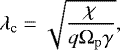 (12)
(12)
where χ is the thermal diffusivity and q is a dimensionless measure of the disk shear (q = 3∕2 for a Keplerian disk). Second, the low-density gas is distorted by the shear motions. The rotation of the inner disk with respect to the protoplanet is faster and the low-density gas thus propagates ahead of the protoplanet. The motion of the outer disk lags behind the protoplanet and so does the hot perturbation. As a result, two hot lobes with decreased density are formed along the streamlines outflowing from the Hill sphere, as described by Benítez-Llambay et al. (2015). The size of the lobes is inherently asymmetric because the corotation between the protoplanet and the sub-Keplerian gas is radially shifted inwards, therefore the outer rear lobe is usually larger and the heating torque should be positive.
Such anadvection-diffusion interplay is indeed observed in Fig. 3, where we find the typical two-lobed distribution of hot underdense gas around the luminous protoplanet and the positive boost of the total torque (Fig. 2) confirms that the outer lobe is slightly more pronounced. The bottom-right panel reveals the magnitude and spatial extent of the temperature excess, as well as its skewed shape in the direction of the disk shear.
However, we make a new observation here concerning the streamlines of the flow that are overlaid in the temperature maps. It is obvious that the hot perturbation significantly changes the topology of the flow with respect to the cold-protoplanet case. U-turn streamlines no longer appear in the depicted part of the disk, the direction of the circulating streamlines changes as they pass the protoplanet, and a new set of spiral-like retrograde streamlines appears.
3.3.2 Vertical plane
It is known that vertical motions play an important role in the structure of circumplanetary envelopes (e.g. Tanigawa et al. 2012; Fung et al. 2015; Ormel et al. 2015; Cimerman et al. 2017; Lambrechts & Lega 2017; Kurokawa & Tanigawa 2018; Popovas et al. 2019). Since previous studies of the heating torque did not investigate the vertical perturbations, we therefore do so here. Figure 4 shows the gas temperature and the velocity field in the vertical plane intersecting the location of the protoplanet. When the protoplanet is cold, there is a vertical stream of gas descending towards the protoplanet and escaping as an outflow through the midplane, in accordance with e.g. Lambrechts & Lega (2017).
However, in the presence of accretion heating the direction of the gas flow above the protoplanet is reverted; it forms an outflowing column while the midplane flow becomes directed towards the protoplanet. Two overturning cells appear on each side of the vertical column (although it is important to point out that no such cells are apparent in the full 3D flow which is discussed later). We notice that the hot perturbation is not spherically symmetric but rather elongated in the direction of the column, indicating that the envelope is not hydrostatic.
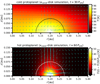 |
Fig. 4 Temperature map around the cold protoplanet at t = 30 Porb (top) and temperature excess around the hot protoplanet at t = 60 Porb (bottom) in the κconst-disk. The verticalplane (perpendicular to the disk midplane) is displayed. The green arrows show the vertical velocity vector field. |
3.3.3 Two- and three-dimensional streamline topology
So far, we have described two new findings that were not incorporated in the existing descriptions of the heating torque (Benítez-Llambay et al. 2015; Masset 2017): the distortion of the streamline topology and the reversal of the vertical motions. The flow direction is directly linked to the heating torque because it determines the redistribution of the hot gas by advection and thus contributes to the shape of the underdense regions. Therefore, we focus on the streamline topology in this section.
The streamlines are calculated using the explicit first-order Euler integrator and the trilinear interpolation of the velocity field. The interpolation allows us to obtain the velocity vector at an arbitrary location within the spherical grid. The size of the integration step is chosen so that the length integrated during a single propagation does not exceed 0.1 of the shortest cell dimension.
We construct 2D and 3D projections of the streamline topologies. For the 2D projections, the streamlines are generated exactly at the midplane where vϕ = 0 and although they provide a useful visualisation, we emphasise that by construction they carry no information about the adjacent vertical flows. For the 3D projections, the streamlines are generated slightly above the midplane (at ϕ = π∕2 − 0.005 rad) to take into account non-zero vϕ.
Figure 5 shows 2D and 3D streamlines in the κconst-disk, again for the exact same simulation stages as in Figs. 3 and 4. In the plots, we distinguish the following types of streamline: first, there are circulating streamlines that do not cross the corotation with the protoplanet. To imagine the direction of the relative motion, we point out that the gas on inner circulating streamlines moves faster than the protoplanet, whereas the gas on outer circulating streamlines lags behind the protoplanet. Second, there are horseshoe streamlines that make a single U-turn and cross the corotation once at each side of the protoplanet. Such streamlines ahead of the orbital motion of the protoplanet form the front horseshoe region and those located behind the protoplanet belong to the rear horseshoe region. To outline the separatrices between the horseshoe and circulating regions, we highlight the critical inner and outer circulating streamlines that are located closest to the protoplanet. Finally, some of our plots contain streamlines that do not fall in any of the aforementioned categories.
When the protoplanet is non-luminous, the 2D midplane streamlines in Fig. 5 do not exhibit any unexpected features. The stagnation point (X-point) of the flow is located within the Hill sphere, which is also intersected by both horseshoe and circulating streamlines. In 3D, we notice that upon making their U-turn, the horseshoe streamlines vertically descend towards the midplane, as already pointed out by Fung et al. (2015) or Lambrechts & Lega (2017). A similar descent is also exhibited by some of the circulating streamlines closest to the protoplanet.
For the hot protoplanet, we now obtain a clear picture of the streamline distortion. In the midplane, the following changes appear:
-
Circulating streamlines cross a smaller portion of the Hill sphere. When passing the protoplanet, they are bent towards it (unlike near the non-luminous protoplanet where they are rather deflected away), which is especially apparent for the critical circulating streamlines.
-
The classical horseshoe streamlines detach from the Hill sphere and make their U-turns at greater azimuthal separations.
-
Part of the streamlines originating in the downstream horseshoe regions is captured inside the Hill sphere where it rotates around the protoplanet in a retrograde fashion.
In 3D, the distortion has the following additional features:
-
The “captured” streamlines are uplifted and form a spiral-like vertical column, outflowing and escaping from the Hill sphere.
-
When the circulating streamlines pass the protoplanet and become perturbed, they are also uplifted. This behaviour is the exact opposite of that seen in the cold-protoplanet situation.
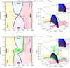 |
Fig. 5 Detailed streamline topology in the κconst-disk simulation. Top row: cold protoplanet at t = 30 Porb. Bottom row:hot protoplanet at t = 60 Porb. Rectangular projection in the spherical coordinates is used to display the disk midplane near the protoplanet (left) and the actual 3D flow (right). The colour of the curves distinguishes individual sets of streamlines: inner circulating (yellow), outer circulating (red), front horseshoe (light blue), rear horseshoe (purple) and other (green). The thick black lines highlight the critical circulating streamlines closest to the protoplanet. The black cross and the ellipse mark the location and Hill sphere of the protoplanet; the black arrows indicate the flow direction with respect to the protoplanet. In 3D figures (right), the dark blue hemisphere corresponds to the Hill sphere above the midplane. Additionally, the insets in the corners of the 3D figures provide a close-up of the upstream outer circulating streamlines viewed from a slightly different angle. The endpoints indicate where the flow exits the depicted part of the space and highlight if the initially coplanar streamlines descend towards the protoplanet (top) or rather rise vertically (bottom). We emphasise that the streamlines in the 3D figures are generated above the midplane and do not directly correspond to those in the 2D figures. |
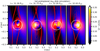 |
Fig. 6 Evolution of the perturbed midplane gas density in the κBL-disk simulation. The corresponding simulation time t is given by labels. Individual snapshots represent the state of gas when the total torque acting on the protoplanet is minimal (left), maximal (third), and oscillating in between (second and right). The streamlines are overplotted for reference. The figure is also available as an online movie, showing the temporal evolution from t = 30–33 Porb. |
3.4 Instability of the heated gas
We now return to the κBL-disk simulation for which we discovered the strong oscillations of the heating torque (Fig. 2).
3.4.1 Evolving underdense lobes
Investigating the evolution of the gas density, we find that the position and size of the underdense lobes never become stationary, as shown in Fig. 6 (see also the online movie). The figure shows a sequence of snapshots corresponding to t = 31.3, 31.75, 32.20 and 32.65 Porb.
The first panel depicts the state when the total torque reaches its first minimum during the beginning of the oscillatory phase. There is a dominant underdense lobe located ahead of the protoplanet while the rear lobe almost disappears. Such a distribution can be easily related to the strong negative torque: the excess of the gas mass behind the protoplanet (and the paucity of mass ahead of it) leads to an azimuthal pull acting against the orbital motion, imposing a negative torque.
When the torque is reversing from negative to positive (second panel), both lobes are similarly pronounced. The rear one seems to be located closer to the protoplanet. The third panel corresponds to the torque maximum. The rear lobe is dominant and thus the overabundance of the gas ahead of the protoplanet makes the torque positive. The final panel shows the state when the oscillating torque is approximately halfway from positive to negative. The gas distribution indeed looks like a counterpart to the second panel since both lobes are again apparent but the front one is now closer to the protoplanet.
The gas redistribution is clearly related to the topology of the streamlines and to the position of the spiral-like flow. We notice that the centre of the captured streamlines undergoes retrograde (“clockwise”) rotation around the protoplanet. One underdense lobe is always associated with this rotating flow. Apparently, the redistribution of the hot gas by advection tends to favour the lobe which is intersected by the majority of the captured streamlines at a given time. In the first panel of Fig. 6, for example, the hot gas is transported more efficiently into the front lobe, creating a strong front-rear asymmetry between the lobes. In the third panel, the situation is exactly the oppositeand the rear lobe is more pronounced.
We point out that the continuous variations of the hot lobes and their alternating dominance are unexpected features of the heating torque which was previously thought to be strictly positive (Benítez-Llambay et al. 2015).
3.4.2 Evolving 2D and 3D streamline topology
We again explore the streamline topology and its changes related to the redistribution of the hot gas. Figure 7 shows the midplane streamlines near the protoplanet for a selection of simulation times between t = 31.3 and 32.15 Porb. The former corresponds to the torque minimum, the latter to the torque maximum. The time intervals between the individual panels are not uniform but are rather selected to highlight the most interesting transitions.
The sequence reveals the following features:
-
In panel a, the streamlines are similar to the steady-state κconst-disk case (bottom of Fig. 5) in several ways, mostly in the detachment of the classical horseshoe streamlines and in the existence of the retrograde streamlines captured from downstream horseshoe regions. But there are also important differences: there are none inner circulating streamlines intersecting the Hill sphere and moreover, a larger part of the captured streamlines originate in the rear horseshoe region while the front horseshoe region is almost disconnected.
-
In panel b, the front horseshoe region becomes entirely disconnected. The captured streamlines originate exclusively in the rear horseshoe region.
-
In panel c, the outer circulating streamlines also stop crossing the Hill sphere. Some of the streamlines that were captured in b now overshoot the protoplanet and make a U-turn ahead of it. The centre around which the captured streamlines enclose becomes shifted behind the protoplanet.
-
In panel d, the front X-point moves closer to the Hill sphere and so do the front horseshoe streamlines. The rear horseshoe region becomes radially narrower and the number of U-turn streamlines overshooting the protoplanet diminishes.
-
In panel e, the front horseshoe region reconnects with the captured streamlines.
-
In panel f, the captured streamlines originate mostly in the front horseshoe region while the rear horseshoe region is evolving towards its disconnection, similarly to what we saw for the front horseshoe region in panels a and b. The centre of the captured streamlines moves inwards from the protoplanet (and will continue to propagate ahead).
Figure 8 shows three selected snapshots of 3D streamlines (t = 31.3, 31.75 and 32.15 Porb) when the oscillating torque is at its minimum (top), grows halfway towards the maximum (middle), and reaches it (bottom). Clearly, the reshaping of the streamline topology that we described for the midplane propagates in a complicated way into the vertical direction as well:
-
In the first panel, the spiraling streamlines of the vertical column are more or less centred above the protoplanet and as they rise above the midplane they penetrate the majority of the Hill sphere.
-
In the second panel, we see the overshooting rear horseshoe streamlines making their U-turns within the Hill sphere. The vertical column of captured streamlines is displaced to the rear of the Hill sphere. As the captured streamlines spiral up, the column tilts towards the Hill sphere. The outer circulating streamlines are strongly uplifted towards colatitudes above the Hill sphere.
-
In the third panel, some uplifted outer circulating streamlines penetrate into the vertical column and by this reconfiguration, the column reconnects with the front horseshoe region while the rear one starts to disconnect.
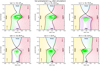 |
Fig. 7 Midplane streamline topology in the κBL-disk simulation. The panels are labelled by the simulation time. The individual types of streamlines are the same as in Fig. 5. The sequence (a–f) represents the transition between the states corresponding to the minimum and maximum of the torque, respectively (see Fig. 2 to relate the panels to the torque evolution). |
3.5 Physical processes distorting the gas flow
In previous sections, we revealed that the gas heating from an accreting protoplanet changes the topology of the flow. Perturbed streamlines have a tendency to bend towards the protoplanet and also to rise vertically. If the perturbations become strong enough, the streamlines can form a vertical spiral. In this section, we investigate the physical processes responsible for such a streamline distortion.
In Sect. 3.5.1, we theorise that the streamline distortion is a result of vorticity perturbations arising because the vigorousaccretion heating renders the circumplanetary gas baroclinic. Confirmation is provided for the steady state of the κconst-disk simulation in Sects. 3.5.2 and 3.5.3. Finally, Sect. 3.5.4 demonstrates that the vertical temperature gradient above the accreting protoplanet is superadiabatic and we also highlight differences between the κconst-disk and the κBL-disk.
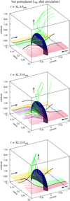 |
Fig. 8 Three-dimensional streamlines in the κBL-disk simulation. Each snapshot is labelled by the simulation time. The panels correspond to the minimum (top) and maximum (bottom) torque and to the state in between (middle). |
3.5.1 Vorticity evolution
The spiral-like structure of the captured streamlines and the bending of nearby circulating streamlines suggests that the vorticity of the flow is modified when the protoplanet becomes hot. The vorticity can be defined via the relation
 (13)
(13)
where ωa is the absolute vorticity and ωr is the relative vorticity in the reference frame corotating with the protoplanet.
Evolution of ωr is described by the vorticity equation in the corotating frame (see Appendix C)
 (14)
(14)
where D∕Dt denotes the Lagrangian derivative. In writing the equation, we neglected the effects of viscous diffusivity (large Reynolds number limit) but otherwise the equation is general.
Regarding the terms on the right-hand side, the first one describes the tendency of vortex tubes to become twisted due to velocity field gradients and the second one characterises the stretching or contraction of vortex tubes due to flow expansion or compression. These first two terms, usually called the twisting and stretching terms, are only important if there is non-zero absolute vorticity already existing in the flow and they can cause its redistribution.
The remaining term on the right-hand side is the baroclinic term. It vanishes in barotropic flows where the pressure and density gradients are always parallel, but since our model is not barotropic, ∇ρ and ∇P can be misaligned, leading to vorticity production or destruction since their cross product can be non-zero. Because ρ near the accreting protoplanet exhibits asymmetric perturbations while P remains roughly spherically symmetric, one can expect non-zero baroclinic perturbations to arise. The respective non-zero vorticity then enhances circulation around a given point of the continuum, twisting the streamlines with respect to the situation unperturbed by accretion heating.
3.5.2 Baroclinic vorticity generation
It is not a priori evident which source term is the most important for the vorticity evolution in our simulations. In Fig. 9, we study the variations of ωr and the source terms of Eq. (14) along a single outer circulating streamline. We compare the situation near the cold and hot protoplanet in the κconst-disk.
Downstream, before the streamline encounters the protoplanet, the situation is similar for the compared cases: the azimuthal and radial vorticity components ωr,θ and ωr,r are negligible, while the polar component ωr,ϕ is non-zero and positive. The positive value of ωr,ϕ correspondsto the inherent vorticity in a flow with the Keplerian shear: taking vr = 0, vϕ = 0 and  , one obtains
  . At the sametime, the source terms are zero because far from the protoplanet there are no strong velocity gradients, no compression and ∇ρ and ∇P are aligned.
To relate the vorticity variation with the streamline distortion close to the protoplanet, let us carry out a thought experiment, considering the fact that the vorticity describes the tendency of the flow to circulate around some point in space. First we focus on the hot-protoplanet case which is the most important for us. First we imagine an observer moving along the critical outer circulating streamline, corresponding to the outer thick black curve in thebottom right panel of Fig. 5. The observer moves with the flow, predominantly in the − θ direction. For this experiment, we dub the directions θ, − θ, r, − r, ϕ and − ϕ as behind, ahead, outwards, inwards, down, and up, respectively. Considering only the streamlines of Fig. 5 originating at r > rp, they initially define a plane at constant ϕ = π∕2 − 0.005 rad and the observer propagates through that plane. When the flow reaches the Hill sphere, the observer studies the instantaneous displacement of nearby gas parcels which corresponds to the deformation of the surface defined by neighbouring streamlines.
According to the bottom panels of Fig. 9, the observer measures ωr,θ > 0 when crossing the Hill sphere. Thus ωr,θ points against the direction of the motion of the observer, forcing the circulation in the local (r, ϕ) plane. The nearby gas parcels must obey the following right-hand rule: when the thumb points in the direction of ωr,θ, wrapping fingers determine the direction of circulation. From the point of view of the observer, an outer gas parcel falls downwards to the midplane and an inner gas parcel rises upwards. This is exactly in accordance with Fig. 5 where streamlines passing the protoplanet are uplifted from the ϕ = π∕2 − 0.005 rad plane and the kick gets stronger with decreasing separation from the protoplanet.
ωr,r only slightly oscillates during the Hill sphere crossing but becomes positive (although relatively small) upstream. Using again the same considerations as above, ωr,r points outwards from the observer after crossing the Hill sphere, promoting circulation in the (θ, ϕ) plane. Using the right-hand rule, a gas parcel ahead of the observer falls downwards and a gas parcel behind the observer rises upwards. In Fig. 5, this is reflected by the streamline topology when the red streamlines rising after the Hill sphere passage suddenly start to fall back towards the midplane.
As for the remaining vorticity component ωr,ϕ, it remains positive during the Hill sphere crossing but acquires a positive boost at first and a more prominent negative perturbation afterwards. The later diminishes the circulation related to shear in the (r, θ) plane. This is only possible if gas parcels near the observer become displaced towards trajectories with smaller shear velocities. In Fig. 5, the streamline topology indeed exhibits such a behaviour because when the red streamlines (and similarly green and yellow ones) pass the protoplanet, they are being bent towards it.
Looking at the source terms, it is obvious that the baroclinic term is responsible for perturbing ωr,θ and ωr,ϕ, while counteracting the twisting term contributing to ωr,r. The importance of the baroclinic term for the flow approaching the hot protoplanet is thus confirmed. Moreover, the perturbation is indeed 3D as each of the studied components is important for the resulting streamline topology.
Comparing the hot-protoplanet case to the cold-protoplanet case, we notice that the evolution of ωr,θ and ωr,ϕ is roughly antisymmetric, as is the evolution of the baroclinic source term. This is consistent with our finding that streamlines near the cold protoplanet are distorted in the opposite manner (they fall towards the midplane and deflect away from the protoplanet). In other words, the baroclinic behaviour of the vicinity of the protoplanet is reverted between the cold- and hot-protoplanet case.
 |
Fig. 9 Evolution of the relative vorticity (first and third row) and balance of the vorticity source terms (second and fourth row) along a single streamline in the κconst -disk simulation. The streamlines for these measurements are chosen from the 3D sets displayed in Fig. 5. For the hot protoplanet (bottom two rows) the extremal outer circulating streamline is selected, and for the cold protoplanet (top two rows) we select an outer circulating streamline with a comparable Hill sphere crossing time. Azimuthal (left), radial (middle), and polar (right) components of the vorticity (black solid curve), and the baroclinic term (blue solid curve), stretching term (orange dashed curve), and twisting term (magenta dotted curve) are displayed using scaled code units. The grey rectangle marks the Hill sphere crossing. We point out that the source terms represent the rate of change of the vorticity and also that the vertical range is not kept fixed among individual panels. |
3.5.3 Baroclinic region
Although we do not repeat the vorticity analysis for the remaining sets of streamlines, it is clear that features of the streamline distortion can be explained by the baroclinic generation of the vorticity. To further support this claim, we compare in Fig. 10 the map of the baroclinic term near the cold and hot protoplanet in the κconst-disk. We plot the polar component of the baroclinic term 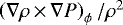 in the midplane. Since the midplane flow is effectively 2D (because vϕ = 0 in midplane), only the polar component of ωr is non-zero and thus also the polar component of the baroclinic term is the most important one.
Figure 10 reveals that the gas is baroclinic near both the cold and hot protoplanet, but for the latter case, the map becomes approximately antisymmetric compared to the cold-protoplanet case, slightly rotated in the retrograde sense and the baroclinic region is more extended.
The existence of the baroclinic region can be explained using the isocontours of constant volume density and isobars. For a barotropic gas (∇ρ∥∇P), any nearby isocontours of constant ρ and P should have the same shape. Wherever the isocontours depart from one another, it means that the local gradients of ρ and P are misaligned and that the baroclinic term is non-zero.
Lookingat the cold-protoplanet case, the isobars and contours of constant density are nearly spherically symmetric. However, we notice that each density isocontour exhibits two bumps and appears to be stretched in the direction where the gas outflows from the Hill sphere. Clearly, these bumps are associated with the cold-finger perturbation that appears in the same location (see Fig. 3). Since the cold fingers are filled with overdense gas, they perturb the local density gradient, causing it to point towards them. At the same time, the isobars remain approximately spherically symmetric.
When the protoplanet is hot, the cold fingers are replaced with hot underdense perturbations. Therefore, the local density gradient tends to point away from them. We can see that this is indeed true because the density isocontours do not exhibit bumps, but rather concavities across the overheated region (compare with Fig. 3). Clearly, thisis the reason why the baroclinic map for the hot protoplanet appears reverted compared to the cold protoplanet.
Summarising these findings, we see that the thermal perturbations associated either with the cold-finger effect or the heating torque makethe circumplanetary region baroclinic. But the influence on the vorticity evolution is the opposite when comparing the cold- and hot-protoplanet cases.
 |
Fig. 10 Maps of the ϕ-component of the baroclinic term in the κconst-disk simulation. The purple isocontours depict several levels of the constant volume density and the green isocontours correspond to the isobars. The levels of the contours are kept fixed between the panels. |
3.5.4 Vertical convection
Although the baroclinic distortion of the gas flow is a robust mechanism, it does not provide a simple explanation as to why the κBL -disk simulation exhibits gas instability whereas the κconst-disk simulation remains stable. We now explore the vertical stability of both disks against vertical convection, considering only the hot-protoplanet limit.
To do so, we employ the Schwarzschild criterion,
 (15)
(15)
where the subscript “rad” denotes the vertical3 temperature gradient found in our simulations and the subscript “ad” denotes the temperature gradient that an adiabatic gas would establish. The ∇ symbol stands for the logarithmic gradient d logT∕d logP, yielding |∇ad,ϕ| = (γ − 1)∕γ for the adiabatic case.
The Schwarzschild criterion is not necessarily a universal way to determine if the disk is unstable to convection. The reason is that convective destabilisations in protoplanetary disks are opposed by diffusive effects (e.g. Held & Latter 2018) and shear motions (Rüdiger et al. 2002). However, to our knowledge there are no convective criteria that would take into account the disk perturbation by the protoplanet, therefore we choose to use the Schwarzschild criterion for its simplicity, keeping the limitations in mind.
Figure 11 shows the vertical velocity field and balance of the Schwarzschild criterion in the vertical direction of the κconst-disk and κBL-disk. Each panel shows a different simulation time and vertical plane. For the κconst-disk, we display t = 60 Porb and the vertical plane intersecting the location of the protoplanet, whereas for the κBL -disk, each plane approximately intersects the centre around which the captured streamlines of Fig. 6 circulate at the given simulation time (t = 31.3, 31.75, 32.2 and 32.65 Porb). In other words, we choose the vertical planes where we expect the most prominent vertical outflow.
The first thing we point out is that the background differs between the studied disks. The background of the κBL -disk is slightly superadiabatic, contrary to the κconst-disk. The difference arises as a result of the opacity laws. As derived by Lin & Papaloizou (1980) and Ruden & Pollack (1991), one can make a qualitative estimate for optically thick regions unperturbed by the protoplanet
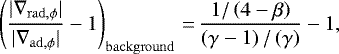 (16)
(16)
where β is the power-law index of the κ ∝ Tβ dependence. In the κconst-disk, β = 0 and thus |∇rad,ϕ|∕|∇ad,ϕ|− 1 ≃−0.17. In the κBL-disk, the Bell & Lin (1994) opacity law in the given temperature range corresponds to water-ice grains and exhibits β = 2, therefore |∇rad,ϕ|∕|∇ad,ϕ|− 1 ≃ 0.67. These estimated values are in a good agreement with the background values of Fig. 11.
The background itself is not convective because vertical convection is usually not self-sustainable unless there is a strong heat deposition within the disk (e.g. Cabot 1996; Stone & Balbus 1996; Klahr et al. 1999; Lesur & Ogilvie 2010) which, however, can be provided by the hot accreting protoplanet in our case. Indeed, looking at the κconst-disk in Fig. 11 (top), the region where we previously identified the most significant temperature excess due to planetary luminosity (compare with Fig. 4) is superadiabatic and the corresponding vertical outflow can be considered convective.
In the κBL-disk simulation, the temperature gradient departs from the adiabatic one even more, and additionally, the excess is no longer centred above the protoplanet itself but rather spans its vicinity. This can be seen from the varying azimuthal coordinate of the displayed vertical planes and also from the radial offset of the highly superadiabatic region in panels 3 and 5.
We summarise the section by speculating that the κBL -disk simulation becomes destabilised because the hot disturbance created by the accreting protoplanet is subject to vertical buoyant forces acting over a more extended region (compared to the κconst-disk). The reason is that the hot disturbance is imposed over an already superadiabatic background. The uplift of the material cannot be compensated for in a stationary manner and eventually the vertical outflow becomes offset with respect to the protoplanet and starts to change its position in a cyclic manner. However, such a description is rather qualitative and precise conditions for triggering the instability should be explored in future works.
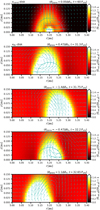 |
Fig. 11 Balance of the Schwarzschild criterion in the vertical planes of the κconst -disk (top) and the κBL-disk (remaining panels). The individual vertical planes are chosen to track the most prominent vertical flow at the given simulation time t (see the main text) and their azimuthal separations from the protoplanet location are given by panel labels (using multiples of the azimuthal span ΔθH of the Hill sphere radius). The colour maps evaluate Eq. (15). Positive values indicate superadiabatic vertical temperaturegradients. The vertical velocity vector field is overlaid in the plots. The half-circles mark the overlap of a given plane with the Hill sphere (the planes in panels 3 and 5 do not overlap with the Hill sphere). |
3.6 Torque oscillation versus opacity gradient
We now perform a partial exploration of the parametric space by varying the opacity gradient within the disk. The aim is twofold: first, we would like to support the claim of the previous Sect. 3.5.4 of the importance of the vertical stratification for the torque oscillations. Second, it is desirable to show that the appearance of torque oscillations in the κBL -disk is not coincidental and that it can be recovered for a wider range of parameters.
We construct six additional disk models with artificial opacity laws that (i) conserve the opacity value at the protoplanet location (1.11 cm2 g−1) and (ii) lead to opacity gradients which are intermediate between the κconst- and κBL-disks. The latter property accounts for the highly unconstrained size distribution of solid particles in protoplanetary disks which manifests itself in a large parametric freedom of the power-law slope of the opacity profile (e.g. Piso et al. 2015).
The first additional set of disks utilises the opacity law which we dub T-dependent:
 (17)
(17)
Similarly to the Bell & Lin (1994) opacity in the water-ice regime, it is exclusively a function of temperature. The temperature  is again azimuthally averaged to disentangle the influence of global opacity gradients (which we focus on) from those related to accretion heating of the protoplanet. We examine the values β = 1.5, 1, and 0.5 to span the range between β = 0 (κconst-disk) and 2 (κBL-disk). The constant of proportionality κ0 is always chosen to recover κ = 1.11 cm2 g−1 at r = ap and ϕ = π∕2 in an equilibrium disk. We find κ0 ≃ 0.0016, 0.014, and 0.122 cm2 g−1 for the respective values of β.
The opacity law used for the second additional set of disks, referred to as r-dependent, is
 (18)
(18)
and we choose δ = 3, 2, and 1 (because δ = 4 leads to an opacity profile similar to the κBL-disk). The motivation for choosing this purely radially dependent opacity law is to distinguish between effects caused by radial and vertical opacity gradients. The latter does not appear when κ = κ(r).
The opacity profiles of these disks in radiative equilibrium are summarised in Fig. 12 which reveals that all radial opacity gradients (top two panels) are indeed shallower compared to the κBL -disk. However, all disks with r-dependent opacities have zero vertical opacity gradient by construction (bottom panel), unlike disks with T-dependent opacities which vertically decrease.
The torque measurements are performed in the same way as in our previous experiments and the results are given in Fig. 13. For disks with T-dependent opacities (top), we find that the torque oscillations appear for all investigated values of β. The oscillation amplitude on the other hand decreases linearly with β and the period becomes slightly shorter as well. In case of r-dependent opacities (bottom), the torque evolution does not strongly depend on δ and exhibits marginal and vanishing oscillations, as in the κconst-disk case.
Since the only qualitative difference between the disks with T-dependent and r-dependent opacities is in the vertical opacity gradient, our torque measurements confirm the importance of the vertical structure for the torque oscillations. The torque oscillates wherever the vertical opacity profile favours superadiabatic vertical stratification and the oscillation amplitude scales with the strength of the opacity-temperature coupling. In the absence of the vertical opacity gradient, the oscillations are not established.
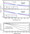 |
Fig. 12 Radial (top two panels) and vertical (bottom) opacity profiles in equilibrium disks which we use to study the torque dependence on the opacity gradients. In the top panels, the individualcases are distinguished by colour and labelled in the legend. The profile of the κBL -disk (solid grey curve) is plotted for comparison. The bottom panel corresponds to the protoplanet location and demonstrates that only thedisks with T-dependent opacities develop a vertical opacity gradient (which is not allowed for r-dependent opacities by construction). |
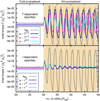 |
Fig. 13 Torque evolution in disks described in Fig. 12. Top panel: disks with T-dependent opacities. Bottom panel: disks with r-dependent opacities. The individual cases are distinguished by colour and labelled in the legend. The evolution from the κBL -disk simulation (solid grey curve) is given for reference. In the top panel, the torque amplitude diminishes with the power-law index of theopacity law, yet the oscillations appear in all studied cases. In the bottom panel, we find that oscillations are rapidly damped. |
3.7 Evolution of a migrating protoplanet
The previous simulations were conducted assuming a fixed orbit for the protoplanet and the static torque was examined. Here we explore whether or not our findings can be readily applied to a dynamical case when the protoplanet is allowed to radially migrate and its semimajor axis evolves. In this section, we focus only on the κBL -disk in which we found the flow instability.
Starting from t = 30 Porb, we release the protoplanet and run the simulation until t = 60 Porb. Figure 14 compares the obtained dynamical torque with the previous result of our static experiments. It is obvious that the oscillating character of the torque is retained and therefore the instability of the flow operates near a moving protoplanet as well. There are differences both in the amplitude and phase of the torque oscillations, but the mean value of the torque over the simulated period of time is 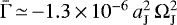 . Although this value is slightly more positive than the static heating torque (
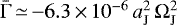 ), it is almost the same as the torque acting on the cold protoplanet (
 ). We thus confirm that in the κBL-disk, the heating torque does not add any considerable positive contribution to the mean torque but causes it to strongly oscillate instead.
The bottom panel of Fig. 14 shows the actual evolution of the semimajor axis of the protoplanet. On average, the protoplanet slowly migrates inwards but this drift is not smooth. The protoplanet exhibits fast periodic inward and outward excursions on an orbital timescale. The migration rate of these individual excursions (not to be confused with the mean migration rate stated above) is ȧ ~ (10−3 au)∕Porb.
Finally, we note that the mean migration rate is not constant, which also corresponds to the varying offset of the dynamical torque with respect to the static torque in Fig. 14. It is likely that the unstable gas distribution around the protoplanet is further affected by the protoplanet’s radial drift.
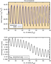 |
Fig. 14 Top: comparison of the static (solid black curve) and dynamical torque (dashed blue curve) acting on the hot protoplanet in the κBL -disk. Bottom: evolution of the semimajor axis in the κBL-disk when the protoplanet is allowed to migrate. The migration is inward and oscillatory. |
4 Discussion
This sectiondiscusses the applicability of our results, draws links to some previous studies, and speculates about possible implicationsfor planet formation. Additionally, we outline possibilities for future work. Although most of them are beyond the scope of thispaper, we at least present several additional simulations in Appendix B to verify the correctness of our model (we study the impact of the luminosity increase, grid resolution, opacity treatment, and computational algorithm on the evolution of torque oscillations).
4.1 Relation to previous works
Our results revealed unexpected perturbations of the gas flow in the vicinity of the protoplanet undergoing strong accretion heating, oneof them being the vertical outflow. The resolution of our simulations was originally tailored for studying the torque and may lack some accuracy close to the protoplanet where the outflow occurs. Follow-up studies should therefore use simulations with a high-resolution protoplanetary envelope, similarly to Tanigawa et al. (2012); Fung et al. (2015); Ormel et al. (2015); Lambrechts & Lega (2017) for example.
It is likely that a critical combination of the opacity κ and luminosity L for a given planetary mass Mp exists for which the vertical outflow is triggered, similarly to the dependences of the heating torque explored by Benítez-Llambay et al. (2015). Popovas et al. (2018, 2019) studied the stability of the circumplanetary envelope during pebble accretion and found that the gas within the Bondi sphere exhibits 3D convective motions, assuming4 L ≃ 1.4 × 1026 erg s−1, Mp = 0.95 M⊕ and κ = 1 cm2 g−1. Lambrechts & Lega (2017) also explored a set of (L, κ, Mp) parameters and their impact on the structure of the circumplanetary envelope. They found the inner region of the envelope to depart from hydrostatic equilibrium when the luminosity exceeds L = 1027 erg s−1 around a Mp = 5 M⊕ core within a κ = 1 cm2 g−1 environment, but they did not identify any vertical outflow. The outflow in our simulations appears for higher L and smaller Mp compared to Lambrechts & Lega (2017). We can therefore assume that our parameters cross the critical ones.
Regarding the baroclinic perturbations, although they are known to produce vortical instabilities in protoplanetary disks (Klahr & Bodenheimer 2003; Petersen et al. 2007a,b; Lesur & Papaloizou 2010; Raettig et al. 2013; Barge et al. 2016), they have rarely been considered in relation to hot protoplanets. For example, Owen & Kollmeier (2017) claim that that hot protoplanets can excite large-scale baroclinic vortices but we do not identify any of those in our simulations. Instead, we find baroclinic perturbations to be responsible for 3D distortion of the gas flow near the protoplanet.
4.2 Implications for the formation of planetary systems
Although the heating torque has previously been thought to be strictly positive and also efficient in high-opacity locations of protoplanetary disks, our paper shows that it can exhibit more complicated behaviour if the temperature dependence of the disk opacity is taken into account. We identified an oscillatory mode of the heating torque in the disk region with κ ∝ T2 and we demonstrated that it can operate even for shallower dependences such as κ ∝ T0.5, albeit with a decreased amplitude. This behaviour resembles the nature of baroclinic and convective disk instabilities which usually operate in the most opaque regions with the steepest entropy gradients but become less effective elsewhere (e.g. Pfeil & Klahr 2019).
It is worth noting that our simulations neglected the effect of stellar irradiation. Stellar-irradiated disks tend to have vertical temperature profiles that are closer to being isothermal (e.g. Flock et al. 2013), unlike disk models used in this work which have rather adiabatic or slightly superadiabatic vertical temperature gradients. On the other hand, even the irradiated disks often contain shadowed regions protected against stellar irradiation; for example behind the puffed-up inner rim (e.g. Dullemond et al. 2001) or between the viscously heated inner disk and a flaredirradiated outer disk (e.g. Bitsch et al. 2013). In such regions, the oscillatory migration could still operate.
For the aforementioned reasons, it is likely that transition zones might exist in protoplanetary disks, separating regions where protoplanets migrate under the influence of the standard positive heating torque and where they undergo oscillatory migration. Migration at the edges of such zones could be convergent, leading to a pileup of protoplanets.
5 Conclusions
By means of3D radiation-hydrodynamic simulations, we investigated the heating torque (Benítez-Llambay et al. 2015) acting on a luminous 3 M⊕ protoplanet heated by accretion of solids. The aim was to compare the torque evolution and physics in a disk with non-uniform opacities (Bell & Lin 1994) with the outcome of a constant-opacity simulation.
We discovered that the gas flow near the protoplanet is perturbed by two mechanisms:
- 1.
The gas advected past the protoplanet becomes hot and underdense. Consequently, a misalignment is created between the gradients of density and pressure within the Hill sphere of the protoplanet. The baroclinic term of the vorticity equation (~∇ρ × ∇P) then becomes non-zero and modifies the vorticity of the flow.
- 2.
The efficient heat deposition in the midplane makes the vertical temperature gradient superadiabatic, thus positively enhancing vertical gas displacements.
The streamline topology exhibits a complex 3D distortion. The most important feature are spiral-like streamlines rising vertically above the hot protoplanet, forming an outflow column of gas escaping the Hill sphere.
In the constant-opacity disk, the vertical outflow is centralised above the protoplanet; it temporarily captures streamlines from both horseshoe regions and such a state is found to be stationary over the simulation time scale. The distribution of the hot gas then remains in accordance with findings of Benítez-Llambay et al. (2015), having a two-lobed structure, and so does the resulting positive heating torque.
In the disk with non-uniform opacity, κ ∝ T2 (typically outside the water-ice line), we find the superadiabatic temperature gradient to be steeper and the distorted gas flow to be unstable. The vertical spiral flow becomes offset with respect to the protoplanet and periodically changes its position, spanning the edge of the Hill sphere in a retrograde fashion. Its motion is followed by the underdense gas and the resulting heating torque strongly oscillates in time. The interplay can be characterised by the following sequence:
- 1.
A stage when most of the captured streamlines originate in the rear horseshoe region and their spiral-like structure is offset ahead of the protoplanet. Therefore the hot gas cumulates ahead of the protoplanet, a dominant underdense lobe is formed there, and the torque becomes negative, reaching the minimum of its oscillation.
- 2.
A stage when the front horseshoe region becomes completely isolated from the captured streamlines. Some of the rear horseshoe streamlines start to overshoot the protoplanet and make U-turns ahead of it. At the same time, the spiral-like structure recedes behind the protoplanet. The lobe from stage 1 starts to decay while a rear lobe starts to grow and the torque changes from negative to positive.
- 3.
Antisymmetric situation to stage 1, when most of the captured streamlines originate in the front horseshoe region, the dominant lobe trails the protoplanet and the torque is positive, reaching the maximum of its oscillation.
- 4.
Antisymmetric situation to stage 2, when the torque decreases from positive to negative and the cycle repeats.
Such an advective redistribution of the hot underdense gas is sustained over the simulation timescale.
We also studied the dependence of the torque oscillations on the opacity gradient and found that they can appear even for κ ∝ T0.5, although their amplitude linearly decreases with the power-law slope of the κ(T) dependence. We also demonstrated that the oscillations would vanish in a disk with zero vertical opacity gradient.
If the protoplanet is allowed to migrate, its mean migration rate is nearly unaffected but the radial drift is not smooth; it is rather oscillatory, consisting of brief inward and outward radial excursions with a characteristic rate of ȧ ~ 10−4 au yr−1.
We discussed possible implications of the oscillating heating torque for planet formation and pointed out that it can affectthe global evolution of hot migrating low-mass protoplanets. During their migration through disk regions withvarying opacities it might be possible for the protoplanets to switch between the standard positive heating torque of Benítez-Llambay et al. (2015) and the positive/negative torque oscillations discovered in this paper.
Movie
Movie of Fig. 6 Access Supplementary Material
Acknowledgements
The work of O.C. has been supported by Charles University (research program no. UNCE/SCI/023; project GA UK no. 624119; project SVV-260441), by the Grant Agency of the Czech Republic (grant No. 18-06083S) and by The Ministry of Education, Youth and Sports from the Large Infrastructures for Research, Experimental Development and Innovations project IT4Innovations National Supercomputing Centre LM2015070. Access to computing and storage facilities owned by parties and projects contributing to the National Grid Infrastructure MetaCentrum, provided under the programme “Projects of Large Research, Development, and Innovations Infrastructures” (CESNET LM2015042), is greatly appreciated.O.C. would like to thank M. Brož and B. Bitsch for useful discussions and also E. Lega who kindly provided her numerical code FARGOCA for comparison simulations. The authors are grateful to an anonymous referee whose insightful ideas helped to improve the manuscript.
Appendix A Modifications of the numerical scheme
We implemented Eqs. (3) and (4) into FARGO3D using their discrete form derived by Bitsch et al. (2013; see their Appendix B). We introduce a minor modification of the numerical scheme, which allows for all the source terms to be accounted for in a single substep. Using the same notation as in Bitsch et al. (2013), the relation between the temperature and radiative energy at t + Δt is
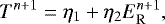 (A.1)
(A.1)
and we redefine
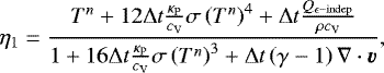 (A.2)
(A.2)
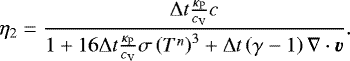 (A.3)
(A.3)
There are two changes with respect to Bitsch et al. (2013). First, the compressional heating is included via the last term in the denominator of Eqs. (A.2) and (A.3). Second, the Qɛ-indep term is a sum of all heat sources that do not depend on ɛ (or T); in our case Qɛ-indep = Qvisc + Qart + Qacc. We note that when necessary, the stellar irradiation term can also be easily included in Qɛ-indep but it is neglected in this work.
Appendix B Supporting simulations
In this appendix, we summarize several additional simulations designed to confirm the robustness of our conclusions.
B.1 Simulation with a smoothly increasing luminosity of the protoplanet
In our main simulations, we usually start the phase with accretion heating abruptly, by instantaneously increasing the luminosity of the protoplanet from L = 0 to the value corresponding to the mass doubling time τ = 100 kyr. Such a sudden appearance of a strong heat source might produce an unexpected behaviour and instabilities by itself. In order to exclude any undesirable behaviour, we repeat the κBL -disk simulation with accretion heating of the protoplanet, but now we linearly increase L from zero at t = 30 Porb to its maximal value over the time interval of 10 Porb.
Figure B.1 shows the measured torque evolution. Clearly, the gradual increase of L has no impact on the final character of the torque, and the oscillations related to the flow reconfigurations inevitably appear.
B.2 Simulation with an increased azimuthal resolution
The resolution in our simulations is motivated by works of Lega et al. (2014) and Eklund & Masset (2017). Although we do not perform extended convergence tests of our own, the resolution should be sufficient to recover a realistic torque value and also a realistic advection-diffusion redistribution of the hot gas near the protoplanet.
However, once the circumplanetary flow becomes unstable, it is no longer clear if the chosen resolution is sufficient. For example, one might argue that the coverage of the Hill sphere by the grid cells in the azimuthal direction is too poor. Here we present an experiment in which we double the number of the grid cells in the azimuthal direction in order to obtain the same coverage of the Hill sphere in all directions. We perform the κBL -disk simulation again, however we shorten the phase without accretion heating to 10 Porb and the phase with accretion heating to 5 Porb.
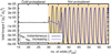 |
Fig. B.1 Torque evolution in the κBL-disk with instantaneously increased luminosity of the protoplanet L (solid black curve; same as in Fig. 2) compared to the κBL-disk with smoothly increasing L (dashed bluecurve). Even before L reaches its maximum value in the latter case, the curves start to overlap. After t = 40 Porb, the agreement is almost exact. |
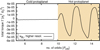 |
Fig. B.2 Torque evolution obtained in the κBL-disk simulation with an increased azimuthal resolution of 2764 cells. The time span of the individual phases is shortened to save computing time. The instability in the presence of the accretion heating is however recovered again. |
The result is shown in Fig. B.2 and demonstrates that the torque oscillations are recovered even when the increased resolution is used. However, the amplitude of the torque oscillations slightly changes, implying that the resolution dependence should be explored more carefully in the future.
B.3 Simulation with the unmodified Bell & Lin opacity table
The simulations of the κBL-disk presented inthis paper are performed with a simplified opacity law of Bell & Lin (1994) (explained in Sect. 2.2). Here we test how the results change if the unmodified opacity law  is used and the dependence on the local values of T and ρ is retained.
Figure B.3 compares the torque evolution in our standard κBL -disk with that in a  -disk. Clearly, the instability occurs in both disks, regardless of whether or not the input values for the opacity function areazimuthally averaged. The only difference is in the torque amplitude which is larger in the
  -disk.
The increased amplitude occurs because if T locally rises, so does the material opacity ( in the givendisk region). Subsequently, the radiative cooling of the hot gas becomes less efficient and T rises even more. As a result, the underdense perturbations related to any temperature excess are more pronounced, leading to the larger amplitude of the torque oscillations.
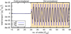 |
Fig. B.3 Comparison of the torque evolutions obtained in the κBL-disk (solid black curve; same as in Fig. 2) and the |

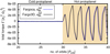 |
Fig. B.4 Comparison of the torque evolutions obtained with two independent codes FARGO3D (solid black curve) and FARGOCA (dashed blue curve). The unmodified
|

B.4 Code comparison
With the aim to confirm that our implementation of the energy equations in FARGO3D is correct and also that the instability of the circumplanetary flow does not arise due to numerical artefacts, we present a comparison simulation obtained with an independent and well-tested radiation hydrodynamic code FARGOCA (Lega et al. 2014). The simulation is performed with the unmodified  opacity law of Bell & Lin (1994).
Figure B.4 compares the torque evolution found using our code with the one obtained with FARGOCA. We can see that the converged torque for the cold protoplanet is in a satisfactory agreement.
When the accretion heating is initiated, the same oscillatory trend is observed with both codes. The curves overlap at first; later they start to depart in terms of the oscillation phase. However, the amplitude remains the same.
Since the converged torques are in agreement and the instability is recovered, we conclude that the differences that we identify in Fig. B.4 arise only because our radiation module in FARGO3D relies on a slightly different numerical scheme (see Appendix A) compared to FARGOCA.
Appendix C Vorticityequation in the corotating frame
For the convenience of the reader, we provide a step-by-step derivation of the vorticity equation. Starting with Eq. (2), we apply the curl on both sides. In the following, we neglect the viscous term (large Reynolds number limit).
The following identities of the vector calculus will be utilised:
 (C.1)
(C.1)
 (C.2)
(C.2)
 (C.3)
(C.3)
 (C.4)
(C.4)
where the last identity holds for scalar functions that are at least twice continuously differentiable.
The curl of the advection term yields
![Mathematical equation: \begin{equation*} \nabla\times\left[\left(\vec{v}\cdot\nabla\right)\vec{v}\right] = \nabla\times\left[\frac{1}{2}\nabla\left(\vec{v}\cdot\vec{v} \right) + \left(\nabla\times\vec{v} \right)\times\vec{v} \right]= \nabla\times\left[\vec{\omega}_{\mathbf{r}}\times\vec{v} \right],\end{equation*}](/articles/aa/full_html/2019/06/aa35334-19/aa35334-19-eq50.png) (C.5)
(C.5)
where we used Eq. (C.1) in writing the first equality, Eq. (C.4) to remove the ~v⋅v term, and we defined the relative vorticity in the corotating frame ωr = ∇ × v. Using Eqs. (C.2) and (C.3), we further obtain
![Mathematical equation: \begin{equation*} \nabla\times\left[\left(\vec{v}\cdot\nabla\right)\vec{v}\right] = \vec{\omega}_{\mathbf{r}}\left(\nabla\cdot\vec{v} \right) + \left(\vec{v}\cdot\nabla \right)\vec{\omega}_{\mathbf{r}} - \left(\vec{\omega}_{\mathbf{r}}\cdot\nabla\right)\vec{v} .\end{equation*}](/articles/aa/full_html/2019/06/aa35334-19/aa35334-19-eq51.png) (C.6)
(C.6)
The curl of the pressure term leads to
 (C.7)
(C.7)
because  (Eq. (C.4)).
When dealing with the gravitational term, it is useful to realise that the centrifugal acceleration can be expressed as  , with the centrifugal potential
  . The curl of a combined force term,
 ![Mathematical equation: $\nabla\,{\times}\,\left[ \nabla\left(\Phi+\Phi_{\mathrm{c}} \right) \right]$](/articles/aa/full_html/2019/06/aa35334-19/aa35334-19-eq56.png) , is zero owing to Eq. (C.4).
, is zero owing to Eq. (C.4).
Finally, we take the curl of the Coriolis acceleration:
![Mathematical equation: \begin{equation*} \nabla\times(2\vec{\Omega}\times\vec{v}) = 2\left[\vec{\Omega}(\nabla\cdot\vec{v}) - \left(\vec{\Omega}\cdot\nabla \right)\vec{v}\right],\end{equation*}](/articles/aa/full_html/2019/06/aa35334-19/aa35334-19-eq57.png) (C.8)
(C.8)
where we removed terms ~∇⋅Ω, ~ ∇Ω because Ω in our simulations is constant.
Recollecting all the terms, we can write the relative vorticity equation
 (C.9)
(C.9)
where we defined the absolute vorticity in the inertial frame ωa = ωr + 2Ω.
References
- Barge, P., Richard, S., & Le Dizès, S. 2016, A&A, 592, A136 [CrossRef] [EDP Sciences] [Google Scholar]
- Baruteau, C., & Masset, F. 2008, ApJ, 672, 1054 [NASA ADS] [CrossRef] [Google Scholar]
- Baruteau, C., Fromang, S., Nelson, R. P., & Masset, F. 2011, A&A, 533, A84 [NASA ADS] [CrossRef] [EDP Sciences] [Google Scholar]
- Bell, K. R., & Lin, D. N. C. 1994, ApJ, 427, 987 [NASA ADS] [CrossRef] [Google Scholar]
- Benítez-Llambay, P., & Masset, F. S. 2016, ApJS, 223, 11 [NASA ADS] [CrossRef] [Google Scholar]
- Benítez-Llambay, P., Masset, F., Koenigsberger, G., & Szulágyi, J. 2015, Nature, 520, 63 [NASA ADS] [CrossRef] [Google Scholar]
- Bitsch, B., Crida, A., Morbidelli, A., Kley, W., & Dobbs-Dixon, I. 2013, A&A, 549, A124 [NASA ADS] [CrossRef] [EDP Sciences] [Google Scholar]
- Brasser, R., Matsumura, S., Muto, T., & Ida, S. 2018, ApJ, 864, L8 [NASA ADS] [CrossRef] [Google Scholar]
- Brož, M., Chrenko, O., Nesvorný, D., & Lambrechts, M. 2018, A&A, 620, A157 [NASA ADS] [CrossRef] [EDP Sciences] [Google Scholar]
- Cabot, W. 1996, ApJ, 465, 874 [NASA ADS] [CrossRef] [Google Scholar]
- Chrenko, O., Brož, M., & Lambrechts, M. 2017, A&A, 606, A114 [NASA ADS] [CrossRef] [EDP Sciences] [Google Scholar]
- Chrenko, O., Brož, M., & Nesvorný, D. 2018, ApJ, 868, 145 [NASA ADS] [CrossRef] [Google Scholar]
- Cimerman, N. P., Kuiper, R., & Ormel, C. W. 2017, MNRAS, 471, 4662 [NASA ADS] [CrossRef] [Google Scholar]
- Coleman, G. A. L., & Nelson, R. P. 2016, MNRAS, 457, 2480 [NASA ADS] [CrossRef] [Google Scholar]
- Cresswell, P., Dirksen, G., Kley, W., & Nelson, R. P. 2007, A&A, 473, 329 [NASA ADS] [CrossRef] [EDP Sciences] [Google Scholar]
- Crida, A., Morbidelli, A., & Masset, F. 2006, Icarus, 181, 587 [Google Scholar]
- de Val-Borro, M., Edgar, R. G., Artymowicz, P., et al. 2006, MNRAS, 370, 529 [NASA ADS] [CrossRef] [Google Scholar]
- Dullemond, C. P., Dominik, C., & Natta, A. 2001, ApJ, 560, 957 [NASA ADS] [CrossRef] [Google Scholar]
- Eklund, H., & Masset, F. S. 2017, MNRAS, 469, 206 [NASA ADS] [CrossRef] [Google Scholar]
- Flock, M., Fromang, S., González, M., & Commerçon, B. 2013, A&A, 560, A43 [NASA ADS] [CrossRef] [EDP Sciences] [Google Scholar]
- Fung, J., & Chiang, E. 2017, ApJ, 839, 100 [NASA ADS] [CrossRef] [Google Scholar]
- Fung, J., Artymowicz, P., & Wu, Y. 2015, ApJ, 811, 101 [NASA ADS] [CrossRef] [Google Scholar]
- Goldreich, P., & Tremaine, S. 1979, ApJ, 233, 857 [NASA ADS] [CrossRef] [MathSciNet] [Google Scholar]
- Held, L. E., & Latter, H. N. 2018, MNRAS, 480, 4797 [NASA ADS] [Google Scholar]
- Klahr, H., & Kley, W. 2006, A&A, 445, 747 [NASA ADS] [CrossRef] [EDP Sciences] [Google Scholar]
- Klahr, H. H., & Bodenheimer, P. 2003, ApJ, 582, 869 [NASA ADS] [CrossRef] [Google Scholar]
- Klahr, H. H., Henning, T., & Kley, W. 1999, ApJ, 514, 325 [NASA ADS] [CrossRef] [Google Scholar]
- Kley, W. 1989, A&A, 208, 98 [NASA ADS] [Google Scholar]
- Kley, W., & Crida, A. 2008, A&A, 487, L9 [NASA ADS] [CrossRef] [EDP Sciences] [Google Scholar]
- Kley, W., Bitsch, B., & Klahr, H. 2009, A&A, 506, 971 [NASA ADS] [CrossRef] [EDP Sciences] [Google Scholar]
- Korycansky, D. G., & Pollack, J. B. 1993, Icarus, 102, 150 [NASA ADS] [CrossRef] [Google Scholar]
- Kretke, K. A., & Lin, D. N. C. 2012, ApJ, 755, 74 [NASA ADS] [CrossRef] [Google Scholar]
- Kurokawa, H.,& Tanigawa, T. 2018, MNRAS, 479, 635 [NASA ADS] [CrossRef] [Google Scholar]
- Lambrechts, M., & Johansen, A. 2012, A&A, 544, A32 [Google Scholar]
- Lambrechts, M., & Johansen, A. 2014, A&A, 572, A107 [NASA ADS] [CrossRef] [EDP Sciences] [Google Scholar]
- Lambrechts, M., & Lega, E. 2017, A&A, 606, A146 [NASA ADS] [CrossRef] [EDP Sciences] [Google Scholar]
- Lega, E., Crida, A., Bitsch, B., & Morbidelli, A. 2014, MNRAS, 440, 683 [NASA ADS] [CrossRef] [Google Scholar]
- Lega, E., Morbidelli, A., Bitsch, B., Crida, A., & Szulágyi, J. 2015, MNRAS, 452, 1717 [NASA ADS] [CrossRef] [Google Scholar]
- Lesur, G., & Ogilvie, G. I. 2010, MNRAS, 404, L64 [NASA ADS] [Google Scholar]
- Lesur, G., & Papaloizou, J. C. B. 2010, A&A, 513, A60 [NASA ADS] [CrossRef] [EDP Sciences] [Google Scholar]
- Levermore, C. D., & Pomraning, G. C. 1981, ApJ, 248, 321 [NASA ADS] [CrossRef] [Google Scholar]
- Li, H., Lubow, S. H., Li, S., & Lin, D. N. C. 2009, ApJ, 690, L52 [NASA ADS] [CrossRef] [Google Scholar]
- Lin, D. N. C., & Papaloizou, J. 1980, MNRAS, 191, 37 [NASA ADS] [Google Scholar]
- Masset, F. S. 2002, A&A, 387, 605 [NASA ADS] [CrossRef] [EDP Sciences] [Google Scholar]
- Masset, F. S. 2017, MNRAS, 472, 4204 [NASA ADS] [CrossRef] [Google Scholar]
- Masset, F. S., & Casoli, J. 2009, ApJ, 703, 857 [NASA ADS] [CrossRef] [Google Scholar]
- Masset, F. S., & Velasco Romero, D. A. 2017, MNRAS, 465, 3175 [NASA ADS] [CrossRef] [Google Scholar]
- McNally, C. P., Nelson, R. P., Paardekooper, S.-J., & Benítez-Llambay, P. 2019, MNRAS, 484, 728 [NASA ADS] [CrossRef] [Google Scholar]
- Mihalas, D., & Weibel Mihalas, B. 1984, Foundations of Radiation Hydrodynamics (New York: Oxford University Press) [Google Scholar]
- Miranda, R., & Lai, D. 2018, MNRAS, 473, 5267 [NASA ADS] [CrossRef] [Google Scholar]
- Morbidelli, A., Crida, A., Masset, F., & Nelson, R. P. 2008, A&A, 478, 929 [NASA ADS] [CrossRef] [EDP Sciences] [Google Scholar]
- Ormel, C. W., & Klahr, H. H. 2010, A&A, 520, A43 [NASA ADS] [CrossRef] [EDP Sciences] [Google Scholar]
- Ormel, C. W., Shi, J.-M., & Kuiper, R. 2015, MNRAS, 447, 3512 [NASA ADS] [CrossRef] [Google Scholar]
- Owen, J. E., & Kollmeier, J. A. 2017, MNRAS, 467, 3379 [NASA ADS] [CrossRef] [Google Scholar]
- Paardekooper, S.-J., & Mellema, G. 2006, A&A, 459, L17 [NASA ADS] [CrossRef] [EDP Sciences] [Google Scholar]
- Paardekooper,S.-J., & Mellema, G. 2008, A&A, 478, 245 [NASA ADS] [CrossRef] [EDP Sciences] [Google Scholar]
- Paardekooper,S.-J., & Papaloizou, J. C. B. 2009, MNRAS, 394, 2283 [NASA ADS] [CrossRef] [Google Scholar]
- Paardekooper,S.-J., Baruteau, C., Crida, A., & Kley, W. 2010, MNRAS, 401, 1950 [NASA ADS] [CrossRef] [Google Scholar]
- Paardekooper,S.-J., Baruteau, C., & Kley, W. 2011, MNRAS, 410, 293 [NASA ADS] [CrossRef] [Google Scholar]
- Petersen, M. R., Julien, K., & Stewart, G. R. 2007a, ApJ, 658, 1236 [NASA ADS] [CrossRef] [Google Scholar]
- Petersen, M. R., Stewart, G. R., & Julien, K. 2007b, ApJ, 658, 1252 [NASA ADS] [CrossRef] [Google Scholar]
- Pfeil, T., & Klahr, H. 2019, ApJ, 871, 150 [NASA ADS] [CrossRef] [Google Scholar]
- Piso, A.-M. A., Youdin, A. N., & Murray-Clay, R. A. 2015, ApJ, 800, 82 [NASA ADS] [CrossRef] [Google Scholar]
- Popovas, A., Nordlund, Å., Ramsey, J. P., & Ormel, C. W. 2018, MNRAS, 479, 5136 [NASA ADS] [CrossRef] [Google Scholar]
- Popovas, A., Nordlund, Å., & Ramsey, J. P. 2019, MNRAS, 482, L107 [NASA ADS] [CrossRef] [Google Scholar]
- Raettig, N., Lyra, W., & Klahr, H. 2013, ApJ, 765, 115 [NASA ADS] [CrossRef] [Google Scholar]
- Rafikov, R. R. 2002, ApJ, 572, 566 [NASA ADS] [CrossRef] [Google Scholar]
- Rein, H., & Liu, S.-F. 2012, A&A, 537, A128 [NASA ADS] [CrossRef] [EDP Sciences] [Google Scholar]
- Rein, H., & Spiegel, D. S. 2015, MNRAS, 446, 1424 [NASA ADS] [CrossRef] [Google Scholar]
- Ruden, S. P., & Pollack, J. B. 1991, ApJ, 375, 740 [NASA ADS] [CrossRef] [Google Scholar]
- Rüdiger, G., Arlt, R., & Shalybkov, D. 2002, A&A, 391, 781 [NASA ADS] [CrossRef] [EDP Sciences] [Google Scholar]
- Semenov, D., Henning, T., Helling, C., Ilgner, M., & Sedlmayr, E. 2003, A&A, 410, 611 [NASA ADS] [CrossRef] [EDP Sciences] [Google Scholar]
- Stone, J. M., & Balbus, S. A. 1996, ApJ, 464, 364 [NASA ADS] [CrossRef] [Google Scholar]
- Stone, J. M., & Norman, M. L. 1992, ApJS, 80, 753 [Google Scholar]
- Tanaka, H., & Ward, W. R. 2004, ApJ, 602, 388 [NASA ADS] [CrossRef] [Google Scholar]
- Tanaka, H., Takeuchi, T., & Ward, W. R. 2002, ApJ, 565, 1257 [NASA ADS] [CrossRef] [Google Scholar]
- Tanigawa, T., Ohtsuki, K., & Machida, M. N. 2012, ApJ, 747, 47 [NASA ADS] [CrossRef] [Google Scholar]
- Ward, W. R. 1986, Icarus, 67, 164 [NASA ADS] [CrossRef] [Google Scholar]
- Ward, W. R. 1991, in Lunar and Planetary Inst. Technical Report, Vol. 22, Lunar and Planetary Science Conference [Google Scholar]
- Ward, W. R. 1997, ApJ, 482, L211 [NASA ADS] [CrossRef] [Google Scholar]
- Yang, L. T., & Brent, R. P. 2002, in Proceedings of the Fifth Conference on Algorithm and Architectures for Parallel Processing., ed. W. Zhou, X. Chi, A. Goscinski, & G. Li (IEEE), 324 [CrossRef] [Google Scholar]
- Yu, C., Li, H., Li, S., Lubow, S. H., & Lin, D. N. C. 2010, ApJ, 712, 198 [NASA ADS] [CrossRef] [Google Scholar]
- Zhu, Z., Hartmann, L., Nelson, R. P., & Gammie, C. F. 2012, ApJ, 746, 110 [NASA ADS] [CrossRef] [Google Scholar]
Public version of the code is available at http://fargo.in2p3.fr/
Public version of the code is available at https://rebound.readthedocs.io/en/latest/
We use the colatitude ϕ to study the vertical gradients because the curvature of spherical coordinates near the midplane does not significantly depart from the true vertical direction.
Greater number of parameters were discussed in Popovas et al. (2018, 2019) but we quote those closest to this paper.
All Figures
|
Fig. 1 Radial profiles of the characteristic quantities in the κconst-disk (dashed bluecurves) and the κBL-disk (solid black curves) after their numerical relaxation over t = 100 Porb. From top to bottom panels: opacity κ, aspect ratio h = H∕r, temperature T and entropy S = P∕ργ. Midplane values are displayed (or used to derive h). The dotted vertical line indicates the orbital distance of the protoplanet, ap = 5.2 au. |
| In the text | |
|
Fig. 2 Temporal evolution of the total torque exerted on the protoplanet (Mp = 3 M⊕) by the κconst-disk (dashed bluecurve) and the κBL-disk (solid black curve). For t ≤ 30 Porb, the protoplanet is not accreting. Its accretion and the respective heating are activated for t > 30 Porb, as also highlighted by a yellow background. While the blue curve evolves as expected, i.e. gains a positive boost when the accretion heating is initiated (Benítez-Llambay et al. 2015), the black curve does not converge and instead exhibits strong oscillations between positive and negative values. The red horizontal dotted line shows the mean value of the oscillating black curve and demonstrates that the heating torque makes the total torque more negative in this case. |
| In the text | |
|
Fig. 3 Hydrodynamic quantities in the midplane of the κconst-disk close to the protoplanet. Top row: cold protoplanet right before the accretion heating is initiated (at t = 30 Porb). Bottom row: steady state of gas around the hot protoplanet (at t = 60 Porb). The figure isconstructed as a Cartesian projection of the spherical grid. The density maps (left) display the perturbation (ρ − ρ0)∕ρ0 relative to the equilibrium disk (t = 0 Porb), the temperature map for the cold protoplanet (top right) shows the absolute values, and the temperature map for the hot protoplanet (bottom right) shows the excess with respect to the cold protoplanet (by subtracting T(t = 30 Porb) from T(t = 60 Porb)). The position of the protoplanet is marked with the cross, the extent of its Hill sphere is bordered by the circle. The green curves (right) show the topology of streamlines in the frame corotating with the protoplanet. In the inertial frame, the protoplanet would orbit counterclockwise. The streamlines outwards from its orbit thus depict the flow directed from y > 0 to y < 0; the inward streamlines are oriented in the opposite direction. A detailed view of the streamlines is provided in Fig. 5 where we also sort them according to their type. |
| In the text | |
|
Fig. 4 Temperature map around the cold protoplanet at t = 30 Porb (top) and temperature excess around the hot protoplanet at t = 60 Porb (bottom) in the κconst-disk. The verticalplane (perpendicular to the disk midplane) is displayed. The green arrows show the vertical velocity vector field. |
| In the text | |
|
Fig. 5 Detailed streamline topology in the κconst-disk simulation. Top row: cold protoplanet at t = 30 Porb. Bottom row:hot protoplanet at t = 60 Porb. Rectangular projection in the spherical coordinates is used to display the disk midplane near the protoplanet (left) and the actual 3D flow (right). The colour of the curves distinguishes individual sets of streamlines: inner circulating (yellow), outer circulating (red), front horseshoe (light blue), rear horseshoe (purple) and other (green). The thick black lines highlight the critical circulating streamlines closest to the protoplanet. The black cross and the ellipse mark the location and Hill sphere of the protoplanet; the black arrows indicate the flow direction with respect to the protoplanet. In 3D figures (right), the dark blue hemisphere corresponds to the Hill sphere above the midplane. Additionally, the insets in the corners of the 3D figures provide a close-up of the upstream outer circulating streamlines viewed from a slightly different angle. The endpoints indicate where the flow exits the depicted part of the space and highlight if the initially coplanar streamlines descend towards the protoplanet (top) or rather rise vertically (bottom). We emphasise that the streamlines in the 3D figures are generated above the midplane and do not directly correspond to those in the 2D figures. |
| In the text | |
|
Fig. 6 Evolution of the perturbed midplane gas density in the κBL-disk simulation. The corresponding simulation time t is given by labels. Individual snapshots represent the state of gas when the total torque acting on the protoplanet is minimal (left), maximal (third), and oscillating in between (second and right). The streamlines are overplotted for reference. The figure is also available as an online movie, showing the temporal evolution from t = 30–33 Porb. |
| In the text | |
|
Fig. 7 Midplane streamline topology in the κBL-disk simulation. The panels are labelled by the simulation time. The individual types of streamlines are the same as in Fig. 5. The sequence (a–f) represents the transition between the states corresponding to the minimum and maximum of the torque, respectively (see Fig. 2 to relate the panels to the torque evolution). |
| In the text | |
|
Fig. 8 Three-dimensional streamlines in the κBL-disk simulation. Each snapshot is labelled by the simulation time. The panels correspond to the minimum (top) and maximum (bottom) torque and to the state in between (middle). |
| In the text | |
|
Fig. 9 Evolution of the relative vorticity (first and third row) and balance of the vorticity source terms (second and fourth row) along a single streamline in the κconst -disk simulation. The streamlines for these measurements are chosen from the 3D sets displayed in Fig. 5. For the hot protoplanet (bottom two rows) the extremal outer circulating streamline is selected, and for the cold protoplanet (top two rows) we select an outer circulating streamline with a comparable Hill sphere crossing time. Azimuthal (left), radial (middle), and polar (right) components of the vorticity (black solid curve), and the baroclinic term (blue solid curve), stretching term (orange dashed curve), and twisting term (magenta dotted curve) are displayed using scaled code units. The grey rectangle marks the Hill sphere crossing. We point out that the source terms represent the rate of change of the vorticity and also that the vertical range is not kept fixed among individual panels. |
| In the text | |
|
Fig. 10 Maps of the ϕ-component of the baroclinic term in the κconst-disk simulation. The purple isocontours depict several levels of the constant volume density and the green isocontours correspond to the isobars. The levels of the contours are kept fixed between the panels. |
| In the text | |
|
Fig. 11 Balance of the Schwarzschild criterion in the vertical planes of the κconst -disk (top) and the κBL-disk (remaining panels). The individual vertical planes are chosen to track the most prominent vertical flow at the given simulation time t (see the main text) and their azimuthal separations from the protoplanet location are given by panel labels (using multiples of the azimuthal span ΔθH of the Hill sphere radius). The colour maps evaluate Eq. (15). Positive values indicate superadiabatic vertical temperaturegradients. The vertical velocity vector field is overlaid in the plots. The half-circles mark the overlap of a given plane with the Hill sphere (the planes in panels 3 and 5 do not overlap with the Hill sphere). |
| In the text | |
|
Fig. 12 Radial (top two panels) and vertical (bottom) opacity profiles in equilibrium disks which we use to study the torque dependence on the opacity gradients. In the top panels, the individualcases are distinguished by colour and labelled in the legend. The profile of the κBL -disk (solid grey curve) is plotted for comparison. The bottom panel corresponds to the protoplanet location and demonstrates that only thedisks with T-dependent opacities develop a vertical opacity gradient (which is not allowed for r-dependent opacities by construction). |
| In the text | |
|
Fig. 13 Torque evolution in disks described in Fig. 12. Top panel: disks with T-dependent opacities. Bottom panel: disks with r-dependent opacities. The individual cases are distinguished by colour and labelled in the legend. The evolution from the κBL -disk simulation (solid grey curve) is given for reference. In the top panel, the torque amplitude diminishes with the power-law index of theopacity law, yet the oscillations appear in all studied cases. In the bottom panel, we find that oscillations are rapidly damped. |
| In the text | |
|
Fig. 14 Top: comparison of the static (solid black curve) and dynamical torque (dashed blue curve) acting on the hot protoplanet in the κBL -disk. Bottom: evolution of the semimajor axis in the κBL-disk when the protoplanet is allowed to migrate. The migration is inward and oscillatory. |
| In the text | |
|
Fig. B.1 Torque evolution in the κBL-disk with instantaneously increased luminosity of the protoplanet L (solid black curve; same as in Fig. 2) compared to the κBL-disk with smoothly increasing L (dashed bluecurve). Even before L reaches its maximum value in the latter case, the curves start to overlap. After t = 40 Porb, the agreement is almost exact. |
| In the text | |
|
Fig. B.2 Torque evolution obtained in the κBL-disk simulation with an increased azimuthal resolution of 2764 cells. The time span of the individual phases is shortened to save computing time. The instability in the presence of the accretion heating is however recovered again. |
| In the text | |
|
Fig. B.3 Comparison of the torque evolutions obtained in the κBL-disk (solid black curve; same as in Fig. 2) and the |
| In the text | |
|
Fig. B.4 Comparison of the torque evolutions obtained with two independent codes FARGO3D (solid black curve) and FARGOCA (dashed blue curve). The unmodified
|
| In the text | |
Current usage metrics show cumulative count of Article Views (full-text article views including HTML views, PDF and ePub downloads, according to the available data) and Abstracts Views on Vision4Press platform.
Data correspond to usage on the plateform after 2015. The current usage metrics is available 48-96 hours after online publication and is updated daily on week days.
Initial download of the metrics may take a while.