| Issue |
A&A
Volume 690, October 2024
|
|
|---|---|---|
| Article Number | A183 | |
| Number of page(s) | 16 | |
| Section | Planets and planetary systems | |
| DOI | https://doi.org/10.1051/0004-6361/202450899 | |
| Published online | 08 October 2024 | |
Gas dynamics around a Jupiter-mass planet
I. Influence of protoplanetary disk properties
1
Université Côte d’Azur, Observatoire de la Côte d’Azur, CNRS,
Laboratoire Lagrange,
France
2
Univ. Grenoble Alpes, CNRS, IPAG,
38000
Grenoble,
France
3
Universitäts-Sternwarte München, Ludwig-Maximilians-Universität,
Scheinerstr. 1,
81679
München,
Germany
4
Collège de France,
11 Pl. Berthelot,
75005
Paris,
France
5
Imperial College London,
Kensington Lane,
London
W1J 0BQ,
UK
6
Department of Earth, Planetary, and Space Sciences, University of California,
Los Angeles,
CA90095,
USA
7
Center for Star and Planet Formation, Globe Institute, University of Copenhagen,
ØsterVoldgade 5-7,
1350
Copenhagen,
Denmark
★ Corresponding author; e-mail: This email address is being protected from spambots. You need JavaScript enabled to view it.
Received:
28
May
2024
Accepted:
3
August
2024
Abstract
Context. Giant planets grow and acquire their gas envelope during the disk phase. At the time of the discovery of giant planets in their host disk, it is important to understand the interplay between the host disk and the envelope and circum-planetary disk properties of the planet.
Aims. Our aim is to investigate the dynamical and physical structure of the gas in the vicinity of a Jupiter-mass planet and study how protoplanetary disk properties, such as disk mass and viscosity, determine the planetary system as well as the accretion rate inside the planet’s Hill sphere.
Methods. We ran global 3D simulations with the grid-based code fargOCA, using a fully radiative equation of state and a dust-to-gas ratio of 0.01. We built a consistent disk structure starting from vertical thermal equilibrium obtained by including stellar irradiation. We then let a gap open with a sequence of phases, whereby we deepened the potential and increased the resolution in the planet’s neighbourhood. We explored three models. The nominal one features a disk with surface density, ∑, corresponding to the minimum mass solar nebula at the planet’s location (5.2 au), characterised by an α viscosity value of 4 10−3 at the planet’s location. The second model has a surface density that is ten times smaller than the nominal one and the same viscosity. In the third model, we also reduced the viscosity value by a factor of 10.
Results. During gap formation, giant planets accrete gas inside the Hill sphere from the local reservoir. Gas is heated by compression and cools according to opacity, density, and temperature values. This process determine the thermal energy budget inside the Hill sphere. In the analysis of our disks, we find that the gas flowing into the Hill sphere is approximately scaled as the product ∑ν, as expected from viscous transport. The accretion rate of the planetary system (envelope plus circum-planetary disk) is instead scaled as √Σv, with its efficiency depending on the thermal energy budget inside the Hill sphere.
Conclusions. Previous studies have shown that pressure-supported or rotationally supported structures are formed around giant planets, depending on the equation of state (EoS) or on the opacity; namely, on the dust content within the Hill sphere. In the case of a fully radiative EoS and a constant dust to gas ratio of 0.01, we find that low-mass and low-viscosity circum-stellar disks favour the formation of a rotationally supported circum-planetary disk. Gas accretion leading to the doubling time of the planetary system of > 105 years has only been found in the case of a low-viscosity disk.
Key words: planets and satellites: gaseous planets / protoplanetary disks / planet-disk interactions
© The Authors 2024
 Open Access article, published by EDP Sciences, under the terms of the Creative Commons Attribution License (https://creativecommons.org/licenses/by/4.0), which permits unrestricted use, distribution, and reproduction in any medium, provided the original work is properly cited.
This article is published in open access under the Subscribe to Open model. This email address is being protected from spambots. You need JavaScript enabled to view it. to support open access publication.
1 Introduction
The discovery of PDS70b and PDS70c, the first protoplanets directly imaged in their host disk (Keppler et al. 2018; Haffert et al. 2019), provides a unique opportunity to gain new insights in the processes of planet formation and evolution and how these giant planets acquired their atmospheric composition (Cridland et al. 2023). PDS70b and c are giant planets located in a large dust-depleted cavity, at 21 and 34 au, respectively. Their properties remain unclear but all studies are in agreement with the assumption of high masses (3–12 MJup Müller et al. 2018; Haffert et al. 2019; Stolker et al. 2020; Wang et al. 2020). Interestingly, both planets are aptly detected in the Hα line and PDS70c is also detected in the UV continuum (e.g. Haffert et al. 2019; Hashimoto et al. 2020; Zhou et al. 2021), indicating ongoing accretion of gas onto the planets and possibly accretion shocks (Aoyama et al. 2018). Spectro-photometric studies show infrared spectral energy distributions, which are notably red and flat, indicating the existence of dust located within the planetary atmosphere or in a surrounding circum-planetary disk (Christiaens et al. 2019; Wang et al. 2021). The presence of small grains around both planets (and in the inner disk within the cavity) is also suggested by hydro-dynamical simulations by Bae et al. (2019). Interestingly, evidence for dust grains co-located with PDS70c and b was found with ALMA sub-millimeter continuum observations (Isella et al. 2019; Benisty et al. 2021). While the emission around PDS70c, closer to the outer protoplanetary disk, is compact and unresolved (at 2 au resolution), the emission around PDS70b, which is located further-in within the dust-depleted cavity, is faint and diffuse, with a morphology that remains unclear. It is thought that PDS70b is starved of dust grains from the outer disk, as they are filtered out by PDS70c (Pinilla et al. in prep.). While both planets seem to be surrounded by dust, the different observational properties of the emissions around PDS70b and c calls for a better understanding of the structure of the material around the planets and, in general, of the conditions for circum-planetary disks to form.
In this context, numerical simulations can guide our understanding and address major questions such as the formation of a circum-planetary disk (CPD, hereafter), its structure and accretion properties. From the numerical perspective studying the gas dynamics around a giant planet is challenging. As giant planets accrete from the protoplanetary disk and part of the gas enters in the Hill sphere, numerical models require us to resolve both the full disk behaviour and the dynamics in the planet’s Hill sphere. This goal is achieved by using nested meshes on grid based codes either on the full disk or with a local approach, namely, shearing sheet approximation (D’Angelo et al. 2003; Klahr & Kley 2006; Machida et al. 2008; Tanigawa et al. 2012; Szulágyi et al. 2014, 2016), non-regular grid geometry in the planet’s Hill sphere (Lambrechts & Lega 2017; Fung et al. 2019; Lambrechts et al. 2019; Schulik et al. 2019, 2020), or using SPH codes (Ayliffe & Bate 2009).
The first studies have been done in 2D models (D’Angelo et al. 2002) and extended to three dimensions as soon as computing capabilities allowed for it. The reason for including the vertical dimension for giant planets is that their Hill radius is comparable to disk scale height and, in fact, vertical motion has been shown to have an important role for a planet’s accretion (see for example Bate et al. 2003; Klahr & Kley 2006; Tanigawa et al. 2012; Szulágyi et al. 2014; Morbidelli et al. 2014). Comparing the numerical results from the literature is not a simple task, as different codes are used and different physical models are involved. Some of the studies consider the isothermal approximation (Machida et al. 2008, 2010; Tanigawa et al. 2012; Szulágyi et al. 2014; Fung et al. 2019; Béthune & Rafikov 2019), while others adopt a more complex equation of state (EoS hereafter) going from adiabatic (Machida et al. 2010; Fung et al. 2019) to fully radiative EoS on inviscid or viscous disks (D’Angelo et al. 2003; Klahr & Kley 2006; Ayliffe & Bate 2009; Szulágyi et al. 2016; Lambrechts & Lega 2017; Lambrechts et al. 2019; Schulik et al. 2019, 2020; Marleau et al. 2023); in this case, the opacity depends on physical disk properties such as the density and the temperature, or is simply considered as constant (Schulik et al. 2020).
A common result of isothermal models is the formation of a CPD around giant planets. All models agree that the gas that reaches the planetary system (planet plus circum-planetary disk) mainly comes from polar regions and flows down towards the planet with a spiral pattern. A highly debated question among the models is whether gas is also accreted from the equatorial direction. In the case of inviscid disks, some authors have shown that gas reaching the planetary system from disk midplane may lose angular momentum due to the torque exerted by the star through the spiral wave (Szulágyi et al. 2014), whilst others (Klahr & Kley 2006; Machida et al. 2008; Tanigawa et al. 2012) have not found any midplane accretion. However, even in the case of midplane accretion, Szulágyi et al. (2014) found that only 10% of the accreted gas comes from disk midplane, while the remaining accretion was due to polar flow.
In contrast, when considering fully radiative EoS, previous studies are not in agreement: some authors find fully rotationally supported CPD (Ayliffe & Bate 2009; Marleau et al. 2023), whilst others report a slow rotation and a pressure supported planetary envelope (Klahr & Kley 2006; Szulágyi et al. 2016; Lambrechts et al. 2019; Krapp et al. 2024). Using the adiabatic approximation, Fung et al. (2019) showed that a spherical pressure supported adiabatic envelope is found instead of a CPD. Therefore, the isothermal and the adiabatic approximations give the two opposite situations of an extremely efficient and inefficient cooling in the planet’s environment and we can expect to find either a pressure-supported envelope or a CPD when considering the more realistic fully radiative EoS model, depending on the planet’s environment.
Concerning the vertical inflowing gas, it is travelling nearly in free fall at supersonic speed in the cases where a rotationally supported CPD is found (Fung et al. 2019; D’Angelo et al. 2003; Marleau et al. 2023) and subsonic speeds are reported for pressure supported adiabatic envelopes (Fung et al. 2019; Béthune & Rafikov 2019). The inflowing gas hits the envelope’s surface or the CPD and if the shocks occurs at a velocity above a given critical value, the emission of hydrogen Hα lines is expected (D’Angelo et al. 2003; Marleau et al. 2023).
The outcome of fully radiative models has been shown to depend on the temperature at the planet’s position (Szulágyi et al. 2016), which can itself be regulated by the opacity (Ayliffe & Bate 2009; Schulik et al. 2019, 2020). More precisely, keeping the gas bound to the planet cold or decreasing the dust-to-gas ratio to have a low opacity in the local environment enhances the rotational support with respect to the pressure support. The gas accretion rate onto the planet seems independent on the rotational support of CPD: typical accretion rates for a Jupiter-mass planet take values of the order of 2–6 × 10⁻⁵ Jupiter masses per year (Bate et al. 2003; Klahr & Kley 2006; Ayliffe & Bate 2009; Machida et al. 2010; Lambrechts et al. 2019; Schulik et al. 2020); with a larger value of 10−4 Jupiter masses per year in the case of a low opacity disk found in Schulik et al. (2020). Even the lower value of 2 × 10⁻⁵ Jupiter masses per year gives a doubling mass time an order of magnitude shorter than typical disk lifetime, enforcing the idea that Jupiter-mass planets emerged late in disk lifetime. A decline of mass accretion rate is expected for planets embedded in wide gaps (Machida et al. 2010). This could be the case of giant planets embedded in low-viscosity disks.
Recently, Nelson et al. (2023) measured accretion rates on Jupiter-mass planets by using a simple hydrodynamical model with star accretion on surface layers induced through angular momentum loss. These authors found accretion rates in the interval [10−7, 4 × 10⁻⁶] Jupiter masses per year. This result does not require giant planets to form later on. Moreover, the study of low-viscosity disks has garnered interest in recent years both from observational constraints (Pinte et al. 2016; Villenave et al. 2022) and from theories revisiting the generation of turbulence in disks via the magneto-rotational instability (Turner et al. 2014). Recent magnetohydrodynamical models (Bai 2017; Béthune et al. 2017) that take into account non-ideal effects have shown that in disk with a low bulk viscosity (α ~ 10−5), gas can be transported to the star by thin accretion layers located at the disk surface at rate compatible with the observed star-accretion rates.
The aim of this paper to describe the dynamics and physical structure of the gas in the immediate vicinity of a giant planet and investigate the role of key properties of the protoplanetary disk, such as the mass or the viscosity in determining the outcome of the CPD and the planet’s accretion rate. We follow a self-consistent approach that goes from the study of the disk structure, whilst also considering the formation of a gap in the protoplanetary disk. This paper is the first of a series of (at least) two papers, with paper II focusing on the chemical delivery of volatile to the planet (Cridland et al. 2024). The paper is organised as follows. In Sec. 2, we present the physics and the numerical models. We also compare global properties of the three disk models with an embedded Jupiter-mass planet. In Sect. 3, we provide details of the gas dynamics focusing on the Hill sphere. Our conclusions are given in Sec. 4.
2 Models
2.1 Physical model
In this work, the protoplanetary disk (PPD hereafter) is treated as a non-self-gravitating gas whose motion is described by Navier-Stokes equations. We used the grid-based fargOCA code (Lega et al. 2014) with a specific non-uniform grid setting introduced in Lambrechts & Lega (2017). We used spherical coordinates (r, φ, θ), where r is the radial distance from the star (which is at the origin of the coordinate system), φ is the azimuthal coordinate measured from the x-axis, and θ is the polar angle measured from the z-axis (the colatitude). The midplane of the disk is located at the equator, ![Mathematical equation: $\[\theta=\frac{\pi}{2}\]$](/articles/aa/full_html/2024/10/aa50899-24/aa50899-24-eq2.png) . We worked in a coordinate system that rotates with the angular velocity of a planet of a mass, mp:
. We worked in a coordinate system that rotates with the angular velocity of a planet of a mass, mp:
![Mathematical equation: $\[\Omega_p=\sqrt{\frac{G\left(M_{\star}+m_p\right)}{r_p{}^3}},\]$](/articles/aa/full_html/2024/10/aa50899-24/aa50899-24-eq3.png)
where M* is the mass of the central star, G is the gravitational constant, and rp is the semi-major axis of a planet assumed to be on a circular orbit. We consider a planet orbiting a Solar-mass star and, therefore, we indicate the mass of the star as M⊙ in the following.
The dynamics of the gas is provided by the integration of the Navier-Stokes equations composed by a continuity equation and a set of three equations for the momenta (Lega et al. 2014). To the Navier-Stokes system of equations, we added an equation for the energy density of the thermal radiation, Er, and that of the internal energy, e = ρcυT, where ρ and T are the gas volume density and the gas temperature, whilst cυ is the specific heat at constant volume. We followed the evolution of both quantities using the so-called two temperature approach (Commerçon et al. 2011):
![Mathematical equation: $\[\left\{\begin{array}{l}\frac{\partial E_{\mathrm{r}}}{\partial t}-\nabla \cdot \boldsymbol{F}=\rho \kappa_p\left(a_r T^4-c E_{\mathrm{r}}\right) \\\frac{\partial e}{\partial t}+\nabla \cdot(e \boldsymbol{v})=-P \nabla \cdot \boldsymbol{v}-\rho \kappa_p\left(a_r T^4-c E_{\mathrm{r}}\right)+Q^{+},\end{array}\right.\]$](/articles/aa/full_html/2024/10/aa50899-24/aa50899-24-eq4.png) (1)
(1)
where ![Mathematical equation: $\[\boldsymbol{F}=\frac{c \lambda}{\rho \kappa_r} \nabla E_{\mathrm{r}}\]$](/articles/aa/full_html/2024/10/aa50899-24/aa50899-24-eq5.png) is the radiation flux vector calculated in the flux limited diffusion approximation (FLD, Levermore & Pomraning 1981) with λ as the flux limiter (Kley et al. 2009). We indicate with κp and κr respectively the Planck and the Rosseland mean opacity, σ is the Stefan-Boltzmann constant, c is the speed of light. In this paper we consider κp = κr (see Bitsch et al. 2013) and use the opacity law of Bell & Lin (1994).
is the radiation flux vector calculated in the flux limited diffusion approximation (FLD, Levermore & Pomraning 1981) with λ as the flux limiter (Kley et al. 2009). We indicate with κp and κr respectively the Planck and the Rosseland mean opacity, σ is the Stefan-Boltzmann constant, c is the speed of light. In this paper we consider κp = κr (see Bitsch et al. 2013) and use the opacity law of Bell & Lin (1994).
We considered an ideal gas of pressure P with equation of state: P = (γ − 1)e for a gas with adiabatic index of γ = 1.4. The terms P∇ · υ and Q+ are the compressional heating and the viscous heating, respectively (Mihalas & Mihalas 1984). We did not include the heating from the central star. This choice allows us to reduce the computational cost with no significant impact on the gas dynamics in the planet vicinity (see Lega et al. 2015). However, the heating from the central star has an impact on the thermal properties of the disk. In Appendix A, we describe the procedure used to find the disk surface temperature that corresponds to the disk aspect ratio in the vicinity if the planet relative to that obtained for a disk heated by the central star.
Disk models parameters.
2.2 Disk models
We modelled a full disk annulus with an azimuthal domain in [−π, π] since we are interested in the analysis of the exchange of gas between the planet’s Hill sphere and the protoplanetary disk. We are also required to trace the gas dynamics on small scales well inside the Hill sphere. For this purpose, we use a non-uniform grid geometry with a grid suitably designed to have small and nearly uniform cells around the planet and large grid-cells further out. This procedure was introduced by Fung et al. (2015) and tested for the code fargOCA by (Lambrechts & Lega 2017; Lambrechts et al. 2019). We remark that our small scales inside the Hill sphere correspond to about 10 Jupiter radii (considering Jupiter’s current radius); therefore, we cannot study the phase of growth of Jupiter nor define a boundary between the planet and the surrounding gas. In this paper, we consider three simulations of a disk with constant viscosity and surface density defined as: ∑ = ∑0(r/rp)−1/2:
(1) The ‘nominal’ case, hereafter referred to as N, for which we consider ![Mathematical equation: $\[\left(\Sigma_0 / M_{\odot} r_p^{-2}\right)=6.67 \times 10^{-4}\]$](/articles/aa/full_html/2024/10/aa50899-24/aa50899-24-eq8.png) , corresponding to about 210g/cm2 at the planet’s location. For this simulation the viscosity is
, corresponding to about 210g/cm2 at the planet’s location. For this simulation the viscosity is ![Mathematical equation: $\[\nu / r_p^2 \Omega_p=10^{-5}\]$](/articles/aa/full_html/2024/10/aa50899-24/aa50899-24-eq9.png) in code units (the value 10−5 in code units corresponds to 1011m2/s or 1015cm2/s and to a value of α = 4 10−3 at the planet’s position of 5.2 au). These disk parameters are the same as those reported in Szulágyi et al. (2016); Lambrechts et al. (2019).
in code units (the value 10−5 in code units corresponds to 1011m2/s or 1015cm2/s and to a value of α = 4 10−3 at the planet’s position of 5.2 au). These disk parameters are the same as those reported in Szulágyi et al. (2016); Lambrechts et al. (2019).
(2) The ‘low-mass’ case, referred to as Lm, in which the disk is ten times less massive than the nominal one.
(3) The ‘low-mass, low-viscosity’ case, referred to as LmLv, where we consider a low-mass disk in which we also consider a ten-times smaller viscosity value. In Table 1, we give the simulation names and the main parameters.
2.3 Disks with embedded planets: Numerical procedure
2.3.1 Set-up
Before inserting the planet, we ran 2D (r, θ) simulations until the disks reach thermal equilibrium. Thermal equilibrium is obtained with a numerical procedure described in Appendix A. We then expanded the disk azimuthally on φ in the interval [−π, π] and restarted our simulations from initial conditions in thermal equilibrium. We embedded a planet of 20 Earth masses in each disk model and smoothly increased (in a time interval of 20 orbits) the mass until the Jupiter mass was reached. The planet is on the midplane at rp = 5.2au and azimuth φ = 0 (or equivalently at (xp, yp) = (5.2, 0) [au]) on a disk of radial domain [2, 13] [au].
2.3.2 Planetary potential
The gravitational potential of the planets on the disk (Φp) is modelled as in Kley et al. (2009) using the full gravitational potential for disk elements having distance d from the planet larger than a fraction ϵ of the Hill radius, and a smoothed potential for disk elements with d < rsm ≡ ϵRH according to:
![Mathematical equation: $\[\Phi_p= \begin{cases}-\frac{m_p G}{d} & d>r_{\mathrm{sm}}, \\ -\frac{m_p G}{d} f\left(\frac{d}{r_{\mathrm{sm}}}\right) & d \leq r_{\mathrm{sm}},\end{cases}\]$](/articles/aa/full_html/2024/10/aa50899-24/aa50899-24-eq10.png) (2)
(2)
with ![Mathematical equation: $\[f\left(\frac{d}{r_{\mathrm{sm}}}\right)=\left[\left(\frac{d}{r_{\mathrm{sm}}}\right)^4-2\left(\frac{d}{r_{\mathrm{sm}}}\right)^3+2 \frac{d}{r_{\mathrm{sm}}}\right]\]$](/articles/aa/full_html/2024/10/aa50899-24/aa50899-24-eq11.png) . We recall that the Hill radius is defined as: RH = rp(mp/M⊙)1/3. We remark that (unlike the case of 2D simulations) there is no physical need for the use of a smoothed potential in 3D simulations since the full gas column is modelled. However, the planetary potential is singular at the planet’s position and numerically handling the function 1/d when d → 0 requires particular care. Specifically, and as shown in Lambrechts et al. (2019), Fig. A.1, a minimal smoothing length of eight grid cells is required to obtain convergent results with respect to the grid resolution. Here, we adopt the practice suggested by Lambrechts et al. (2019) of doubling the resolution when halving the smoothing length with a multi-phase prescription. In the first phase (A hereafter), we use a moderate resolution (Nr, Nφ, Nθ) = (228, 680, 32) on a uniform grid. In this way, we can benefit from the large time step provided by the FARGO algorithm Masset (2000). At this stage, we have about ten grid-cells in a Hill diameter and therefore we use a large smoothing length for the gravitational potential: ϵ = 0.8 RH. After the planet’s growth, we continue the simulation for additional 80 orbits to let the gap open. Although the gaps have not converged on this integration time (Schulik et al. 2019), the runaway growth timescale is very short, compared to the viscous timescale required for gaps to reach their steady state. Figure 1 (left column) shows the radial density profiles for the three models at the end of phase A. The density of the Lm and LmLv cases has been multiplied by 10 in order to superpose the background unperturbed profiles and appreciate the differences in the gap’s depth and width. We remark that in the low-mass case, the gap is deeper than in the nominal one because the disk has a smaller aspect ratio (see Fig. A.1 bottom panels). In the low viscosity case, the gap is wider than in the other two models (as expected).
. We recall that the Hill radius is defined as: RH = rp(mp/M⊙)1/3. We remark that (unlike the case of 2D simulations) there is no physical need for the use of a smoothed potential in 3D simulations since the full gas column is modelled. However, the planetary potential is singular at the planet’s position and numerically handling the function 1/d when d → 0 requires particular care. Specifically, and as shown in Lambrechts et al. (2019), Fig. A.1, a minimal smoothing length of eight grid cells is required to obtain convergent results with respect to the grid resolution. Here, we adopt the practice suggested by Lambrechts et al. (2019) of doubling the resolution when halving the smoothing length with a multi-phase prescription. In the first phase (A hereafter), we use a moderate resolution (Nr, Nφ, Nθ) = (228, 680, 32) on a uniform grid. In this way, we can benefit from the large time step provided by the FARGO algorithm Masset (2000). At this stage, we have about ten grid-cells in a Hill diameter and therefore we use a large smoothing length for the gravitational potential: ϵ = 0.8 RH. After the planet’s growth, we continue the simulation for additional 80 orbits to let the gap open. Although the gaps have not converged on this integration time (Schulik et al. 2019), the runaway growth timescale is very short, compared to the viscous timescale required for gaps to reach their steady state. Figure 1 (left column) shows the radial density profiles for the three models at the end of phase A. The density of the Lm and LmLv cases has been multiplied by 10 in order to superpose the background unperturbed profiles and appreciate the differences in the gap’s depth and width. We remark that in the low-mass case, the gap is deeper than in the nominal one because the disk has a smaller aspect ratio (see Fig. A.1 bottom panels). In the low viscosity case, the gap is wider than in the other two models (as expected).
We continue the simulation (phase B) for additional 25 orbits using a regular grid with resolution (Nr, Nφ, Nθ) = (456, 1360, 64) in the three directions. The smoothing length is smoothly reduced with respect to phase A down to 0.4 RH.
2.3.3 Boundary conditions
In the azimuthal direction, we used periodic boundary conditions; whereas in the radial direction, we used evanescent boundaries to minimise the wave reflections (de Val-Borro et al. 2006). The reference fields (density, velocity, and gas energy) for evanescent boundaries are those that result from the thermal equilibrium obtained running 2D (r, z) axi-symmetric simulations, as described in Appendix A. In the vertical direction at the disk surface, we considered reflecting boundaries for the velocity components. We also copied the density from the neighbours active cells and set the temperature at the values Tb (as computed in Appendix A). To limit the computational time, we modelled a single disk hemisphere by using a mirror symmetry at the midplane.
2.3.4 Increase of numerical resolution
In the next phase (C hereafter), we used the nonuniform grid geometry (with a number of grid-cells: (Nr, Nφ, Nθ) = (298, 1598, 65)) on a disk annulus of radial domain of r/rp = [0.6, 1.4] (or [3.1, 7.3] [au]) with rp = 5.2 [au]). The grid has finest resolution of ![Mathematical equation: $\[\frac{\Delta r}{r_p}=0.0013\]$](/articles/aa/full_html/2024/10/aa50899-24/aa50899-24-eq12.png) in the three dimensions, close to the planet’s position. The spacing is quasi-constant in the Hill sphere, increases quadratically and has a maximum resolution ratio of 6 in the radial direction (with 10 and 2.5 in the azimuthal and in the vertical directions, respectively, not shown). The number of grid-cells in a Hill radius is of 50. We discuss the convergence of results with respect to resolution and smoothing length in Appendix B. The integration annulus fully contains the gap and the radial domain for evanescent boundary conditions, as seen in Fig. 2.
in the three dimensions, close to the planet’s position. The spacing is quasi-constant in the Hill sphere, increases quadratically and has a maximum resolution ratio of 6 in the radial direction (with 10 and 2.5 in the azimuthal and in the vertical directions, respectively, not shown). The number of grid-cells in a Hill radius is of 50. We discuss the convergence of results with respect to resolution and smoothing length in Appendix B. The integration annulus fully contains the gap and the radial domain for evanescent boundary conditions, as seen in Fig. 2.
The reference fields for the evanescent boundaries are the gas fields inherited by those computed at the end of phase B. Because of the non-uniform geometry of the grid in azimuth, we cannot use the FARGO algorithm in phase C; thus, the simulations take a longer time and we ran them for an additional ten orbits. The smoothing length in phase C is reduced with respect to phase B down to ϵ = 0.2 RH in 1 orbital period (corresponding to 10 grid-cells in the smoothing lenght). All of the figures in the following are snapshots at five orbital periods out of a total of ten orbital periods for this phase. From phase A to phase C, we increased the resolution and reduced the smoothing length: more gas is accreted in the planet vicinity (Fig. 1, top right panels). In Fig. 1 (middle-right panel), we observe averaged temperatures similar to the results of phase A on the coarsely grained grid, along with a huge increase (of a factor of 5–20) in the temperature at the planet’s position. This increase in temperature near the planet follows from the higher spacial resolution, along with the deeper potential and the fact that the main source of heating is compression (Lambrechts et al. 2019). The midplane temperature suddenly drops at the boundary of the Hill sphere; however, small temperature spikes are observed near this boundary in the three models due to the intersection of the selected (azimuthal) slice with the spiral wake (as we show in the next sections). We can already see from this study that local properties of temperature and density in the Hill sphere of a giant planet that has opened a gap depend on such disks parameters as the mass and the viscosity.
3 Gas dynamics in the Hill’s sphere
In this section, we provide a detailed description of the dynamics in the planet’s vicinity and quantify the amount of gas that flows through the Hill sphere as well as the accretion rate in the Hill sphere. In a follow-up paper (Cridland et al. 2024), we will present the chemical evolution of gas along streamlines computed in this work.
To focus on the dynamics in the planet’s vicinity, we worked in the planetocentric reference frame and used either Cartesian coordinates (x, y, z) or spherical coordinates (R, ϕ, ϑ), with R representing the radial distance of the planet, ϕ the azimuthal angle in [0: 2π], where the x-axis, namely, ϕ = 0, marks the Sun-planet direction; ϑ is the colatitude in the interval [0: π/2], with π/2 indicating the planet’s equatorial plane (corresponding to the disk’s midplane) and 0 indicating the pole of the sphere. In Fig. 3, we provide the density field at the disk midplane (left panels) and the azimuthally averaged temperature field (right panels) represented on the plane ![Mathematical equation: $\[(\tilde{R}, z) \equiv(R \sin (\vartheta), R \cos (\vartheta))\]$](/articles/aa/full_html/2024/10/aa50899-24/aa50899-24-eq13.png) for the three models N (top), Lm (middle) and LmLv (bottom). The velocity field (υx, υy) is over-plotted on the background midplane density with white arrows. On the right panels, the velocity field is azimuthally averaged and density weighted as follows:
for the three models N (top), Lm (middle) and LmLv (bottom). The velocity field (υx, υy) is over-plotted on the background midplane density with white arrows. On the right panels, the velocity field is azimuthally averaged and density weighted as follows:
![Mathematical equation: $\[<X>_\rho=\frac{\int_0^{2 \pi} \rho X \mathrm{d} \phi}{\int_0^{2 \pi} \rho \mathrm{d} \phi},\]$](/articles/aa/full_html/2024/10/aa50899-24/aa50899-24-eq14.png) (3)
(3)
where < X > accounts for both components (< υR >, < υz >). The colours of the arrows correspond to the vertical component < υz >ρ in units of the sound speed.
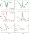 |
Fig. 1 Radial density profiles (top), azimuthally and vertically averaged temperature (middle), and disk aspect ratio (bottom) profiles for the three models at the end of phase A (left) and C (right). The grey dashed lines indicate the boundary of the Hill sphere and the black dotted line the position of the planet. The density of the Lm and LmLv cases has been multiplied by 10 in order to superpose the density background and appreciate the differences in the gap’s depth and width. We notice that in the LmLv case a large amount of gas is accumulated in a radial domain corresponding to the Hill sphere. This is not gas accumulated around the planet but it is the signature of the libration region around the L4 and L5 Lagrangian points not being depleted yet (a known fact in the case of low-viscosity disks). In the middle panel, the midplane temperature is over-plotted with same colours (dashed) on a slice at the planet’s azimuth φ = 0. The higher resolution associated with the deepening of the potential (decreasing smoothing) results in a huge temperature increase up to [1600, 1100, 600] K in the nominal model, the Lm case, and the LmLv model, respectively. In the bottom panel, we remark that it is only in the nominal case that the formation of the gap modifies the aspect ratio considerably. |
3.1 Midplane views
On the plot displaying the density midplane, we clearly see the spiral wake as an over-dense region that shrinks and becomes very thin when moving from the nominal to the LmLv case. The central massive region (envelope) extends to about 0.5 RH, gas is subsonic inside the envelope; whereas it approaches the wake at supersonic speed and is then deviated and slowed at subsonic speed after shock with the wake. We remark that the density structure is similar to the one described in Schulik et al. (2020, see their Fig. 3) for similar protoplanetary disk initial conditions (same viscosity and twice the smaller surface density at the planet’s location), but with a small opacity value of 0.01g/cm2. The wake structure seems not to depend on the opacity, however, the region inside 0.4 RH is in our case almost not rotating. This is typical of pressure-supported envelopes and by lowering the opacity, Schulik et al. (2020) found a rotationally supported structure inside 0.4 RH (and strong spiral wakes in the CPD). In the middle and bottom panels (Lm and LmLv cases), in addition to the spiral wake, we observe additional spiral arms: this is a sign that in these cases the gas surrounding the planet forms a rotationally supported structure or CPD with its tidal spiral arms. When the gas approaches the proto-planet, its motion is deviated by the gravity of the planet. From the literature, we have the definition of three regions (Machida et al. 2008, 2010; Tanigawa et al. 2012) corresponding to classical circulation (also called a pass-by region) and horseshoe motion at distances of >RH, along with a third region for distances of R<RH (called atmospheric region), where the gas is highly perturbed by the planet.
Inside the Hill sphere, we can identify the region where the gas is bound to the planet through energy considerations. Actually, the gas escapes the planet’s potential well if its total energy is larger than the effective potential at the Hill radius: ![Mathematical equation: $\[\Phi_H=-G m_p / R_H-3 / 2 \Omega_p^2 R_H^2\]$](/articles/aa/full_html/2024/10/aa50899-24/aa50899-24-eq15.png) ; here, the second term is the centrifugal contribution in the local approximation (Hill’s equations). Therefore, we can say that the gas is bounded where E ≤ 0 with the specific energy defined as:
; here, the second term is the centrifugal contribution in the local approximation (Hill’s equations). Therefore, we can say that the gas is bounded where E ≤ 0 with the specific energy defined as:
![Mathematical equation: $\[E=\frac{v^2}{2}+c_v T+\Phi_p-\frac{3}{2} \Omega_p^2 x^2-\Phi_H.\]$](/articles/aa/full_html/2024/10/aa50899-24/aa50899-24-eq16.png) (4)
(4)
The zero-level energy contour (black line in the left panels of Fig. 3) shows that the gas is bounded to the planet up to a distance of about 0.4 RH, with a spherical geometry in the N case and with an elongated or disk like structure on the Lm and LmLv cases.
In the left panels of Fig. 3, we have also plotted forward (full lines) and backward (dashed lines) integration for the set of initial conditions of Table 2 projected on the midplane (z = 0), using the 2D velocity fields components (υR, υ&phis). Ignoring the vertical motion, the flow pattern emphasises the influence of the wake on the gas motion. In the top panel (nominal case), after being deviated by the shock with the spiral wake, the brown and pink lines according to the velocity field are further deflected near the Lagrangian point, L1, at approximately x = −0.6, y = 0.1 RH, and reach the boundary of the hot envelope at about 0.4 RH. On average the radial motion of the midplane is directed inward, gas moves towards the hot central envelope and, in the full 3D case (Fig. 3, top-right) is then lifted up. A consequent depression in the midplane will keep the gas moving toward the hot envelope (“green” and “magenta” streamlines), while the others (‘cyan’, ‘black’, and ‘orange’) pass further away from the planet and have a typical horseshoe motion.
In the Lm case, the brown and pink lines are deviated by the wake, have about half a rotation around the planet and are bent again by respectively the CPD spiral arm and the wake and finally leave the Hill region, while the green and magenta lines spiral out and are kinked at each rotation by both the wake and the CPD spirals. A similar behaviour is observed in the LmLv case, with the majority of streamlines entering the Hill sphere participating to horseshoe motion.
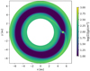 |
Fig. 2 Vertically integrated density of the simulated nominal disk (simulation N in Table 1) in the high-resolution phase (phase C, see text) with non-uniform grid geometry. We clearly see the spiral arms originating at the planet position (xp, yp) = (5.2, 0) [au], revealing the interaction between the planet and the disk. The disk annulus fully contains the gap and slightly extends over the edges. |
3.2 Vertical views
The contour levels plotted in Fig. 3, right panels correspond to the vertical component of the specific angular momentum, j, in a non rotating frame centered on the planet, normalised over the Keplerian angular momentum relative to the planet. More precisely, we have:
![Mathematical equation: $\[j=\frac{< v_\phi \tilde{R}>_\rho+\Omega_p \tilde{R}^2}{\sqrt{G m_p \tilde{R}}},\]$](/articles/aa/full_html/2024/10/aa50899-24/aa50899-24-eq17.png) (5)
(5)
with ![Mathematical equation: $\[\tilde{R}\]$](/articles/aa/full_html/2024/10/aa50899-24/aa50899-24-eq18.png) being the cylindrical radius. In the nominal model, along the polar directions, the gas has less than 30% of the Keplerian angular momentum and flows quasi-vertically towards the planet with a subsonic sound speed – as previously reported in the adiabatic approximation (Fung et al. 2019; Béthune & Rafikov 2019). The in-fall speed further decreases when the gas approaches the hot envelope at about z ~ 0.5[RH]. The gas is bound to the planet inside a spherical envelope of radius 0.4 Hill radii (black line showing the zero energy contour, according to Eq. (4) in Fig. 3, top-right panel). This is typical of a pressure-supported envelope in agreement with the finding of Szulágyi et al. (2016); Lambrechts et al. (2019); Fung et al. (2019). Within the envelope, the gas speed is negligible with respect to the values observed at larger distances.
being the cylindrical radius. In the nominal model, along the polar directions, the gas has less than 30% of the Keplerian angular momentum and flows quasi-vertically towards the planet with a subsonic sound speed – as previously reported in the adiabatic approximation (Fung et al. 2019; Béthune & Rafikov 2019). The in-fall speed further decreases when the gas approaches the hot envelope at about z ~ 0.5[RH]. The gas is bound to the planet inside a spherical envelope of radius 0.4 Hill radii (black line showing the zero energy contour, according to Eq. (4) in Fig. 3, top-right panel). This is typical of a pressure-supported envelope in agreement with the finding of Szulágyi et al. (2016); Lambrechts et al. (2019); Fung et al. (2019). Within the envelope, the gas speed is negligible with respect to the values observed at larger distances.
When looking at the Lm, LmLv cases, we see that gas flows quasi-vertically at supersonic speed in the region bound by the line with 0.3 Keplerian angular momentum in the Lm case and on a larger fraction of the Hill sphere in the LmLv case. In the Lm case, we observe a dense quasi-spherical envelope of a radius of ~0.2[RH] and a thick disk that is partially supported by pressure. The separation between the envelope and the surrounding disk can approximately be set at ~0.2[RH]: for larger distances, the angular momentum gets larger than 60% of the Keplerian value. In the LmLv case, the rotational support increases to 80% of the Keplerian one at a distance of ![Mathematical equation: $\[\tilde{R}\]$](/articles/aa/full_html/2024/10/aa50899-24/aa50899-24-eq21.png) > 0.2[RH]. In the region bounded to the planet and delimited by the zero energy contour (black line in the right panels of Fig. 3), the averaged motion has negligible velocity with respect to the rest of the Hill sphere. The disk structure appears to shield the gas entering in the Hill sphere at low altitude by deviating it, lifting it up (middle right panel of Fig. 3) above the disk structure, and then moving it radially towards the planet, where it falls almost vertically when the angular momentum is low. We describe the dynamics in the planetary system in Sec. 3.4.
> 0.2[RH]. In the region bounded to the planet and delimited by the zero energy contour (black line in the right panels of Fig. 3), the averaged motion has negligible velocity with respect to the rest of the Hill sphere. The disk structure appears to shield the gas entering in the Hill sphere at low altitude by deviating it, lifting it up (middle right panel of Fig. 3) above the disk structure, and then moving it radially towards the planet, where it falls almost vertically when the angular momentum is low. We describe the dynamics in the planetary system in Sec. 3.4.
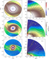 |
Fig. 3 Parameter details for all three models. Left: midplane density field interpolated in cartesian planeto-centric coordinates(x, y) = (R cos(ϕ), R sin(ϕ)) in units of the Hill radius). The cartesian components (υx, υy) of the midplane velocity field are plotted with arrows. The coloured lines are straightforward (full) and backward (dashed) integration of streamlines obtained with the 2D midplane velocity field. Right: azimuthally averaged density field interpolated in planeto-centric coordinates and represented in |
![Mathematical equation: $\[(\tilde{R}, z)=(R \sin (\vartheta), R \cos (\vartheta))\]$](/articles/aa/full_html/2024/10/aa50899-24/aa50899-24-eq19.png)
![Mathematical equation: $\[\tilde{R}\]$](/articles/aa/full_html/2024/10/aa50899-24/aa50899-24-eq20.png)
3.3 Rotational support
The fraction of pressure support with respect to rotational support of a planetary system depends on the cooling efficiency in the Hill sphere (Fung et al. 2019). Ayliffe & Bate (2009) had previously shown that the rotational support increases when decreasing the opacity and this result was recently confirmed in a detailed study by Schulik et al. (2020). Here, we use the Bell & Lin opacity k(ρ, T) for our three models with a dust-to-gas ratio of 0.01. Although the inner and denser part of the planetary envelope may be convective (Zhu et al. 2021), in the outer part, or in the CPD forming region, cooling is mainly radiative (Fung et al. 2019; Krapp et al. 2024). Radiative cooling can be quantified by computing the timescale over which radiation is diffused over the Hill sphere. Following the definition of Bitsch & Kley (2010) we compute:
![Mathematical equation: $\[\tau=\frac{R_H^2}{D_r},\]$](/articles/aa/full_html/2024/10/aa50899-24/aa50899-24-eq22.png) (6)
(6)
where Dr is a radiative diffusion coefficient in the optically thick limit:
![Mathematical equation: $\[D_r=\frac{4 c a T^3}{3 c_v \rho^2 k(\rho, T)}.\]$](/articles/aa/full_html/2024/10/aa50899-24/aa50899-24-eq23.png)
In Fig. 4 we show, as a function of the radial distance from the planet, quantities averaged on spherical planetocentric shells, according to:
![Mathematical equation: $\[F(R)=\frac{1}{2 \pi R^2} \int_0^{2 \pi} \int_0^{\pi / 2} f(R, \theta, \phi / 2) R^2 \sin (\vartheta) \mathrm{d} \vartheta \mathrm{d} \phi,\]$](/articles/aa/full_html/2024/10/aa50899-24/aa50899-24-eq24.png) (7)
(7)
where the function, f, is the cooling timescale in units of orbital periods τ/T (top-left), the opacity (top right), and the volume density and temperature (bottom panels).
The inner region up to 0.1 RH has a high density and opacity values larger than 1 cm2/g for the three models (see Fig. 4) with a moderate decrease of the opacity inside 0.1 RH, where the temperature is higher than 1000° and the opacity decreases because of gas ionisation processes. The radiative cooling timescale is of the order of 103 orbital periods for the three models. At distances greater than 0.3 RH from the planet, τ decreases to values smaller that the dynamical timescale for both the Lm and LmLv cases. In a recent paper, Krapp et al. (2024) proposed a necessary condition for the formation of a CPD depending on the value of the radiative cooling timescale. According to this condition, a CPD forms when the cooling time is of the same order or smaller than the orbital period at the tidal truncation radius: ≃0.3 RH. Although we do not have the same definition of τ as in Krapp et al. (2024), this condition is fullfilled by the LmLv case and marginally fulfilled in the Lm case where the disk structure is thick and partially supported by pressure.
3.4 Streamlines
A detailed description of gas dynamics in the planet’s vicinity is given via the description of streamlines in Machida et al. (2008); Bitsch & Kley (2010); Tanigawa et al. (2012) in the case of isothermal and adiabatic models. With the aim of comparing the gas dynamics in our three models. we consider in this section a set of initial conditions on the Hill sphere (see Table 2 and Fig. 3 for projections on the disk midplane and on the vertical slice).
Streamlines give the motion of gas parcels for quasi-stationary velocity fields. We checked this requirement by comparing the velocity fields at different snapshots on our hydrodynamical integration, which cover nine orbits of Jupiter around the star. For the streamlines, we integrated the velocity field up to ten Jupiter orbits forwards and to two Jupiter orbits backwards. Figure 5 reports the streamlines on a portion of the space slightly larger than the Hill sphere for an integration time of about four Jupiter orbits. On the Hill sphere, we have plotted the radial gas flow rate in planetocentric coordinates: negative values correspond to gas inflow and positive values correspond to outflow (red and blue points, respectively, in Fig. 5). From a simple consideration of the flow sign, we see that gas inflow dominates quasi totally in the Lm and LmLv cases (red regions), whereas a large fraction of the sphere is dominated by outflow (blue regions) in the nominal case. We provide quantitative values of inflow and outflow rate on the Hill sphere as a function of z/RH in Sec. 3.5.
As a first global comment, we can observe that in the N case gas entering at high latitude tends to remain trapped and rotate around the planet, either exiting at high altitude or slowly approaching the planet’s envelope. In the other two cases, a larger number of streamlines are trapped in the planetary system and a more flattened disk structure is observed for the LmLv case, with respect to Lm one. We remark that a larger internal energy budget inside the Hill sphere as for the N case (see Fig. 4 bottom panels) seems to have a key role in determining the fraction of gas accreted in the planetary region with respect to the total gas entering in the Hill sphere. We provide a quantitative study in Sec. 3.5.
In the following, we describe the behaviour of single streamlines by also looking at quantities reported on Fig. 6, where we can appreciate the projected path of streamlines on the x − y global disk as well as the evolution with time of their z and radial components relative to the planet. The dashed lines on the left panels of Fig. 6 correspond to backward integration: we see that in all cases, the gas approaching the Hill sphere comes from U-turn motion passing close to the planet; namely, close to Lagrangian points L1 and L2, from the inner or outer branch of the horseshoe region (in agreement with the findings of Machida et al. 2008, 2010).
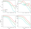 |
Fig. 4 Parameter details for all three models. Top-left: radiative diffusion timescale (from Eq. (6)). Top-right: opacity. Bottom-left: volume density. Bottom right: temperature. All the quantities are obtained through averages over spherical shells centred on the planet. |
3.4.1 Nominal case
In the nominal case, the initial conditions that are very close to the planet’s pole (‘dark blue’ and ‘green’ streamlines) gas enter deep into the envelope and is accreted (see also Fig. 6, top-middle panel), although very low density is carried by gas at high z values. We consider that the gas carried by a streamline is accreted when it enters the region gravitationally bound to the planet (shown by the black lines in Fig. 3). Not all of the gas entering the Hill sphere close to the planet’s pole is accreted, in fact we can see that the ‘magenta’ line, which has an initial value of z/rH very close to the ‘green’ one, but different x and y positions (see Fig. 3, left panel) escapes from the Hill sphere. Precisely, in this case, the gas has a short residence in the Hill sphere moving at lower z values and then is lifted higher up and leaves the Hill sphere reaching the outer disk region (Fig. 6, top row). The computation stops when a streamline reaches the computational domain’s boundaries. Starting further down at z/rH = 0.6 and z/rH = 0.35 (respectively, ‘cyan’ and ‘black’ streamlines), the gas is lifted up in z, according to the direction of the vectors in Fig. 3 (top-right panel). In the longer integration presented in Fig. 6, top panels, the gas transits to the outer disk (‘cyan’ streamline), whereas it re-enters the Hill sphere (‘black’ streamline) after a horseshoe orbit and, finally, transits into the inner disk (Fig. 6, top left panel). A similar behaviour occurs with respect to the ‘orange’ streamline starting at z/rH = 0.1: the gas makes a U-turn in the Hill region (similar to the midplane streamline of Fig. 3, top-left) followed by an horseshoe orbit, then again approaches the Hill sphere, entering at higher z values at about t = 8 orbital periods; finally, it leaves the horseshoe region and reaches the disk’s upper boundary (see Fig. 6, top panels).
For streamlines with initial conditions that are very close to the midplane, we observe: a close approach to the bounded region at d ≃ 0.4RH and a few rotations around the planet that are similar to the corresponding midplane streamline (‘pink’ line). Then the gas is lifted up and transits to the outer disk remaining at large z values (Fig. 6, top panels). Gas starting on the midplane, but at a x y position close to the L1 Lagrangian point (‘brown’ streamline), is deflected and remains bounded at a distance of about 0.4 Hill radii; namely, at the planet’s envelope boundary (Fig. 6, top-right panel). We notice that the dynamical behaviour is similar to the one observed for the corresponding midplane streamline of Fig. 3 (top left); however, in the full 3D velocity field, the gas is lifted up to about 0.4 Hill radii (Fig. 6, top middle panel) and then oscillates vertically whilst rotating around the planet (as indicated by the small period oscillations in Fig. 6, top (middle and right panels). If the gas entering in this case from the midplane carries small dust particles, it will then pollute the planet’s envelope.
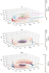 |
Fig. 5 3D representation of streamlines with initial conditions on the Hill sphere (see Table 2). The colour bar corresponds to planeto-centric mass flow rate on the Hill surface. The sign is negative for mass inflow and positive for mass outflow. The total integration time is short (about four Jupiter orbits) in order to make this plot clear. The evolution of the same streamlines on a longer integration allows us to follow the dynamics on a projected plane (x/RH, y/RH) and to appreciate the evolution of the distance with respect to the planet in Fig. 6. |
3.4.2 The Lm and LmLv cases
For the other two cases, the dynamics appear very different: the majority of streamlines are trapped in a toroidal disk structure with an outer bound at about 0.4 RH (slightly larger than the tidal truncation radius) and an inner bound at about 0.25 RH. To explain the path of such streamlines, we show the velocity field for distances <0.5RH in the (![Mathematical equation: $\[\tilde{R}\]$](/articles/aa/full_html/2024/10/aa50899-24/aa50899-24-eq25.png) , z) plane with normalised vectors (Fig. 7). The vector colours correspond to the norm of
, z) plane with normalised vectors (Fig. 7). The vector colours correspond to the norm of ![Mathematical equation: $\[\left(v_{\tilde{R}}, v_z\right)\]$](/articles/aa/full_html/2024/10/aa50899-24/aa50899-24-eq26.png) . The norm of the vectors cover a range of about five orders of magnitude, with smaller values inside the planet’s envelope where the gas is bounded. Gas that shocks the envelope (‘dark blue’, ‘green’, and ‘magenta’ streamlines) at about z ~ 0.2 and z ~ 0.12 (for the (Lm and LmLv cases, respectively) is deviated and trapped in circulating motion in the (
. The norm of the vectors cover a range of about five orders of magnitude, with smaller values inside the planet’s envelope where the gas is bounded. Gas that shocks the envelope (‘dark blue’, ‘green’, and ‘magenta’ streamlines) at about z ~ 0.2 and z ~ 0.12 (for the (Lm and LmLv cases, respectively) is deviated and trapped in circulating motion in the (![Mathematical equation: $\[\tilde{R}\]$](/articles/aa/full_html/2024/10/aa50899-24/aa50899-24-eq27.png) , z) plane (toroidal motion in the full 3D field). Initial conditions making a U-turn far from the planet as the ‘yellow’ and ‘black’ streamlines undergo rapid transit, as observed for the corresponding midplane streamlines of Fig. 3 (middle- and bottom-left panels). The ‘brown’ streamline is deflected by the wake and enters in the inner protoplanetary disk in the LmLv case, whereas it is captured in the disk structure in Lm case (Figs. 5 and 6, middle and bottom panels). When we observe the ‘brown’ streamline, as computed with the midplane velocity field in the Lm case, we see two important deviations when the gas encounters the dense spiral wake, which eventually makes it leave the Hill sphere. Using the full 3D velocity field, the encounter with the wake also modifies the motion in the vertical direction and lifts up the gas (as described in Schulik et al. 2019, Fig. 14, and explained as baroclinic kicks). At the encounter with the outer wake, the streamlines are deviated again and appear to be finally trapped in the disk region. A similar behaviour is observed for the ‘pink’ streamline in the Lm case. Despite the complexity of 3D motion in the Hill sphere, we can conclude by saying that the accretion of gas entering in the Hill sphere is favoured in the Lm and LmLv cases. Here, the gas is colder outside the planet’s envelope with respect to the nominal case, which has a larger internal energy budget inside the Hill sphere (see also Fig. 4, bottom panels).
, z) plane (toroidal motion in the full 3D field). Initial conditions making a U-turn far from the planet as the ‘yellow’ and ‘black’ streamlines undergo rapid transit, as observed for the corresponding midplane streamlines of Fig. 3 (middle- and bottom-left panels). The ‘brown’ streamline is deflected by the wake and enters in the inner protoplanetary disk in the LmLv case, whereas it is captured in the disk structure in Lm case (Figs. 5 and 6, middle and bottom panels). When we observe the ‘brown’ streamline, as computed with the midplane velocity field in the Lm case, we see two important deviations when the gas encounters the dense spiral wake, which eventually makes it leave the Hill sphere. Using the full 3D velocity field, the encounter with the wake also modifies the motion in the vertical direction and lifts up the gas (as described in Schulik et al. 2019, Fig. 14, and explained as baroclinic kicks). At the encounter with the outer wake, the streamlines are deviated again and appear to be finally trapped in the disk region. A similar behaviour is observed for the ‘pink’ streamline in the Lm case. Despite the complexity of 3D motion in the Hill sphere, we can conclude by saying that the accretion of gas entering in the Hill sphere is favoured in the Lm and LmLv cases. Here, the gas is colder outside the planet’s envelope with respect to the nominal case, which has a larger internal energy budget inside the Hill sphere (see also Fig. 4, bottom panels).
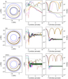 |
Fig. 6 Projection of the streamlines of Fig. 5 on the planetocentric x − y plane (left). The blue contours give the boundaries of the disk. Gas approaching the Hill sphere can have a rapid transit phase in the horseshoe region and be released in the inner or the outer disk trapped in the planetary system. Vertical evolution of streamline with respect to time (middle). Evolution of the distance with respect to the planet as a function of time (right). The dashed lines correspond to backward integration: in the left panel we see that gas approaching the Hill sphere comes from U-turn motion passing close to the planet from the inner or outer branch of the horseshoe region. |
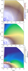 |
Fig. 7 Same as Fig. 3, right panels showing a zoom close to the planetary system. Vectors of components |
![Mathematical equation: $\[\left(v_{\tilde{R}}, v_z\right)\]$](/articles/aa/full_html/2024/10/aa50899-24/aa50899-24-eq28.png)
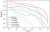 |
Fig. 8 Absolute value of the inflow and outflow mass rate as a function of z on the Hill sphere. In the Lm and LmLv cases the mass inflow is larger than the mass outflow except very close to the midplane which appears decreating. Instead, in the N case, the Hill sphere is accreting up to z = 0.2[RH] and for z > 0.7[RH]. In all the models, the contribution to the total mass flow in the Hill sphere becomes negligible at z > 0.8[RH]. |
Total mass inflow, ![Mathematical equation: $\[\left|\dot{M}_i\right|\]$](/articles/aa/full_html/2024/10/aa50899-24/aa50899-24-eq29.png) and outflow,
and outflow, ![Mathematical equation: $\[\dot{M}_o\]$](/articles/aa/full_html/2024/10/aa50899-24/aa50899-24-eq30.png) rates.
rates.
3.5 Accretion
From the values of mass flow rate (plotted on the Hill sphere in Fig. 5), we have a qualitative view of regions of gas inflow and outflow. We sum these values on the azimuthal direction to provide the total inflow ![Mathematical equation: $\[\dot{M}_i(z)\]$](/articles/aa/full_html/2024/10/aa50899-24/aa50899-24-eq36.png) and outflow mass flow rate
and outflow mass flow rate ![Mathematical equation: $\[\dot{M}_o(z)\]$](/articles/aa/full_html/2024/10/aa50899-24/aa50899-24-eq37.png) as a function of z[RH].
as a function of z[RH].
The resulting values are plotted in Fig. 8, taking the absolute value for the inflow rate. The difference between the inflow and the outflow mass rate will give the net accretion rate, simply called the ‘accretion rate’ in the following. In the Lm and LmLv cases (Fig. 8), the mass inflow is larger than the mass outflow except very close to the midplane. In other words, very close to the midplane the flow is decreating and the rest of the Hill sphere is accreting. Instead, in the N case, the Hill sphere is accreting up to z = 0.2[RH] and for z > 0.7[RH]. In all the models, the contribution to the total mass flow in the Hill sphere becomes negligible for z > 0.8[RH]. The total mass flow in and out of the Hill sphere and the resulting accretion rate are reported in [M⊕/yr] in Table 3.
We can now quantify the accretion rate inside the Hill sphere using the whole time series of data at our disposal. More precisely, we first compute the total mass mR(t) contained on semi-spheres of radius, R, centred on the planet with R going from the 0.01 to 1 Hill radius. We have a total integration time of ten orbits (phase C; see Sec. 2) and the first orbit is used to smoothly reduce the smoothing length. Therefore, we obtained the mass accretion rate from a linear interpolation of the function 2mR(t) (where the factor of 2 gives the whole mass on the sphere) over the remaining nine orbits. In Fig. 9, we plot the accretion rate in Earth masses per year. At the Hill radius, we also plot the total rate of inflow and the accretion rate from Table 3. We observe the good agreement among the accretion rates computed through radial flow on a single time snapshot and the one obtained through interpolation over nine orbits.
In Fig. 9, we notice that below 0.3 Hill radii for the nominal case (0.2 and 0.1 Hill radii for the Lm and LmLv cases, respectively), the accretion rate suddenly decreases and becomes negligible when approaching the planet. We can consider the interior envelope to be slowly contracting and accreting on larger timescales, with respect to our short integration time.
The accretion rate reaches a constant maximal value close to the boundary of the zero energy region (see Fig. 3 and Eq. (4)). This means that gas accreted by the planet piles up in the outer envelope in the N case, and in the CPD in the other two cases; in agreement with our dynamical study.
We observe that in the nominal case, the rate of inflow is of ~0.1M⊕/yr (Table 3, in agreement with Lambrechts et al. (2019, Fig. 2) whilst the accretion rate is of ~0.029M⊕/yr. This is due to the large exchange of gas in the Hill sphere and corresponds to the qualitative description we described in the previous section, via the streamlines.
Instead, in the Lm case, the rate of inflow (~0.011M⊕/yr, Table 3) is marginally higher than the accretion rate (0.009M⊕/yr, Table 3). Therefore, although there is a difference of about a factor of 10 in the total inflow rate between the nominal and the Lm case, as we expect for a viscous transport proportional to ∑ν, there is only a factor of 3 in difference for the accretion rate between the two cases. This result was not expected, since the accretion is considered to behave proportionally to the mass inflow rate; however, we have seen that the accretion depends on the dynamics in the Hill sphere and this changes drastically from the nominal case in comparison to the other two cases, which appear to accrete the in flowing gas more efficiently. Precisely, the accretion appears to be efficient also in the LmLv case, with an accretion rate of 0.0015M⊕/yr for a total inflow rate of 0.0023M⊕/yr. From the viscous disk evolution, the quantity of gas that may be supplied by the disk and can flow onto the planet is proportional to ∑ν. The mass inflow on the Hill sphere provided in Table 3 actually scales as expected based on viscous evolution. Instead, for the net accretion rate in the Hill sphere, we have obtained a scaling ![Mathematical equation: $\[\propto \sqrt{\Sigma} \nu\]$](/articles/aa/full_html/2024/10/aa50899-24/aa50899-24-eq38.png) .
.
The accretion rate inside the Hill sphere is often used to infer the mass doubling time of the planet (or of the planetary system when considering the envelope and the circum-planetary disk). In our case, the Jupiter-mass-doubling time is of the order of a few 104 of years, as previously reported in the literature, for both the N case and the low-mass disk case. Therefore, the typical scenario of a Jupiter-mass planet entering runaway accretion late in the lifetime of a protoplanetary disk remains valid when considering disks less massive than MMSN at the planet’s location.
In the case of a low-viscosity disk, the mass doubling time increases by an order of magnitude. Thus, it is only in the low-viscosity case that a giant planet may enter in runaway accretion earlier in the disk’s lifetime to achieve the same final mass.
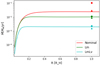 |
Fig. 9 Accretion rate as a function of the distance to the planet in the Hill sphere computed interpolating the time series of the mass contained in a sphere of radius R over 9 planet’s orbital periods (see text). For each case, we report the rate of inflow (circles) and the accretion rate on the Hill sphere (triangle), as computed on a snapshot at five orbital periods (see Table 3). |
4 Conclusion
Using 3D hydrodynamical simulations with a fully radiative equation of state, we have studied the dynamical properties of gas in the Hill sphere of a Jupiter-mass planet in three different protoplanetary disks configurations. The first features a disk with a surface density corresponding to the minimum mass solar nebula (at the planet’s location), characterised by constant viscosity, equivalent to having an alpha parameter of 4 × 10⁻³ at the location of the planet. The second disk model differs from the nominal one in mass, with a surface density that is ten times smaller than the nominal one and same viscosity; whilst in the third model, we also reduce the viscosity value by a factor of 10.
During gap formation, giant planets accrete gas inside the Hill sphere from the local reservoir. Gas is heated by compression and cools according to opacity, density, and temperature values. This process determines the thermal energy budget inside the Hill sphere. We can then describe the characteristics of the planetary system and the dynamics in the Hill sphere when the gas has reached a quasi-stationary state.
In the nominal case, a pressure-supported envelope forms, as already reported in the literature (Ayliffe & Bate 2009; Szulágyi et al. 2016; Fung et al. 2019) and gas cools on timescales that are larger than the orbital period on the whole Hill sphere. In the other cases, we observe an envelope and a CPD-like structure supported partially by pressure and partially by rotation. A necessary condition for the formation of a rotational supported structure was recently given in Krapp et al. (2024) based upon the requirement that the cooling time scale at the tidal truncation radius must be comparable to (or shorter than) one orbital period at the planet’s location. We show that our disk model with low surface density and and low viscosity satisfies this criterion, whilst the low surface density case marginally satisfies it; here, the disk structure in the region 0.2–0.4 RH is indeed quite heavily supported by pressure. The dynamics inside the Hill sphere is also shown to depend on the total energy budget, with the gas being accreted preferentially from midplane in the nominal case and lifted up to colder layers, leaving the Hill sphere preferentially at an altitude of 0.3 < z < 0.7 RH. In the other cases, the gas enters in the Hill sphere and accretes on the planetary envelope except for z values very close to the midplane where the radial motion of the gas (relative to the planet) is positive. The polar accretion channel exists in all the cases although a very small fraction (5% in the N case and 1% in the Lm and LmLv cases) of the accreted gas comes from polar directions with z > 0.8 RH.
In all the cases, a hot envelope is formed in the planet’s vicinity extending to ~0.4 RH, ~0.2 RH and ~0.1 RH, respectively, in the (1) nominal, (2) low-mass, and (3) low-mass+low-viscosity cases. A similar result of giant planets forming an envelope (and eventually a disk structure) that is limited to a fraction of the Hill sphere was also found in Schulik et al. (2020); Krapp et al. (2024).
To form a rationally supported structure or CPD for our nominal disk parameters it is necessary to reduce the opacity (Schulik et al. 2020). In a reduced opacity environment the building blocks for satellite formation may be planetesimals captured in the CPD (Ronnet & Johansen 2020). In this paper, we kept the dust to gas ratio to usual circum-stellar disk values and considering that, although dust is filtered at the planet’s outer gap edge, particles coupled to the gas are free to cross the gap; thus, this may allow the opacity to remain at disk values (Morbidelli et al. 2023).
Although we are limited in resolution and a finite smoothing length, we observe that by increasing the resolution, the inner envelope becomes hotter and denser; at the same time, the properties in the outer part of the Hill sphere remain basically unchanged, so that our results seem to be robust with respect to resolution and smoothing length (Appendix B and Szulágyi et al. 2016). Concerning the accretion rate and the planet’s mass doubling time, our results are consistent with the literature in the nominal and low mass cases.
In particular, we have shown that the scaling of the net accretion rate among the three models behaves as ![Mathematical equation: $\[\sqrt{\Sigma} \nu\]$](/articles/aa/full_html/2024/10/aa50899-24/aa50899-24-eq39.png) . Therefore, only reducing the mass does not significantly increase the mass-doubling time. Low-viscosity disks instead favour a significant increase in the mass-doubling time.
. Therefore, only reducing the mass does not significantly increase the mass-doubling time. Low-viscosity disks instead favour a significant increase in the mass-doubling time.
When considering the low-viscosity disk case, we must remark that viscous transport gives a star accretion rate of ~10−9 M⊙ per year, which is low with respect to observed values of 10−7, 10−8 M⊙ per year (Hartmann et al. 1998; Manara et al. 2016). Star accretion on surface layers, as provided by MHD models, offers a mechanism for disks with low bulk viscosity to have star accretion rates consistent with the observed values. Recently, Nelson et al. (2023) measured accretion rates on Jupiter-mass planets by using a simple hydrodynamical model with star accretion on surface layers induced through angular momentum loss (with a rate of ~10−8 M⊙ per year in magnetised winds). These authors monitored the gas entering in the Hill sphere of a Jupiter-mass planet by varying the thickness of the accretion layer and found a mass-doubling timescale going from 0.2 to 10 Myrs with larger values for very thin accretion layers. The value obtained in this work for the Jupiter doubling time of the planetary system in the LmLv case is of about 0.2 Myr, consistent with the case of gas radially transported across the whole column density in the (Nelson et al. 2023). Applying the procedure presented here on models with thin accretion layers is beyond the scope of this paper and will be undertaken in a future study.
In a follow-up paper (Cridland et al. 2024) we explore the chemical evolution of the gas along streamlines and the resulting chemical structure of the gas in the vicinity of the planet. The aforementioned dependence of the gas temperature on the spatial resolution could change the chemical structure of the gas in the planet’s neighbour and modify the energy content of any molecular line emission that would emanate from near the planet. However, when reaching temperatures above 2000 K by increasing the resolution and further deepening the potential, the model should take into account hydrogen dissociation, which is not included in this work. One example of an equation-of-state adapted to take into account the endothermic reaction of hydrogen dissociation was done through the reduction of the adiabatic index by Fujii et al. (2019). The authors observed temperatures exceeding 104 K in the few grid cells with very deep gravitational potential in cases where a CPD is formed. This is an indication that performing higher resolution studies with a deeper potential would mainly affect the innermost regions close to the planet. However, we consider that further numerical experiments with improved models that take into account hydrogen dissociation, as well as observations, are needed. This will help to better constrain the properties of the gas surrounding embedded planets.
Acknowledgements
We thank an anonymous referee for constructive suggestions that helped improving the manuscript. M.B. and A.C. received funding from the European Research Council (ERC) under the European Union’s Horizon 2020 research and innovation programme (PROTOPLANETS, grant agreement No. 101002188). A.M. is grateful for support from the ERC advanced grant HolyEarth N. 101019380. This work was granted access to the HPC resources of IDRIS under the allocation 2023 A0140407233 and 2024 A0160407233 made by GENCI. E.L. wish to thank Alain Miniussi for maintenance and re-factorisation of the code FARGOCA.
Appendix A Thermal structure
Disks that differ in mass and viscosity have also a different vertical thermal structure. To obtain a coherent description of the thermal structure, we included stellar irradiation in our models using the numerical prescription provided in Bitsch et al. (2014) and performed 2D (r, z) axisymmetric simulations. We considered a solar-mass star with a surface temperature of 4370°K, a radius of 1.5 solar radii, and a disk annulus that extends in the interval r/rp = [0.4, 9] (or r = [2.08, 45.9] au). In the vertical direction the disk extends by 20° over the midplane. We considered a resolution of (Nr, Nθ) = (528, 82).
In our 3D simulations we did not consider stellar irradiation (Eq. 1), in order to have reasonable computational times and to limit the amount of CPUs. However, we can mimic the thermal equilibrium structure obtained in disks heated by the star, by suitably fixing the disk surface temperature.
To this purpose, we ran test cases in which we imposed different values of the boundary temperature, Tb, at the disk surface. The simulations have a resolution of (Nr, Nθ) = (228, 32) on a disk annulus extending radially in the interval r/rp = [0.4, 2.5] and vertically by about 7° over the midplane1.
Figure A.1, left shows the equilibrium midplane temperature (top) and the disk aspect ratios (bottom) for the nominal N model including the stellar heating and for the four test cases without stellar heating. In the inner part of the disk, the values of the aspect ratio are very similar for disks with and without stellar heating (see also Bitsch et al. 2013). This means that viscous heating dominates over the stellar irradiation up to 7–8 au. Beyond 10 au, the irradiated disk is flared, while the disk with Tb = 10 °K collapses to small H/r at large radii, as is typical of disks without stellar heating. We mimicked the flaring by imposing a temperature at the disk’s surface higher than Tb = 10 °K. For the nominal model, a value of Tb = 40 °K nicely fits the temperature structure of the stellar irradiated disk. We remark that the planet position in the paper (vertical black dotted line in Fig. A.1) is at the boundary of the region dominated by viscous heating.
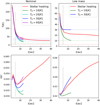 |
Fig. A.1 Midplane temperature (top) and disks’ aspect ratio (bottom) as a function of radial distance from the host star for 2D simulations for the nominal and Lm cases (left and right, respectively). The red lines include the effect of stellar irradiation. The other simulations have no stellar heating and differ in the boundary temperature, Tb, at disk’s surface. The value of Tb that allows us to recover the profile of the stellar irradiated disk is used for 3D simulations of in the rest of the paper. Horizontal dotted lines in the top plots correspond to the values of Tb in the simulations. The vertical black dotted line marks the position of a Jupiter-mass planet in the paper. |
When considering the Lm disk (Fig. A.1, right), the viscous heating, proportional to ∑, dominates only in a very narrow region at the inner disk boundary (Fig. A.1, bottom right), and the planet’s location is in the part of the disk where stellar heating dominates. The boundary temperature required to mimic stellar irradiation is Tb = 30 °K. In the model with low viscosity (LmLv), the stellar heating dominates in the full disk range that we are considering. We remark that the amount of energy absorbed in the disk from the star’s photons depends on the density and the opacity and therefore the Lm and LmLv disks have the same thermal structure2. Therefore, we also considered a value of Tb of 30 °K in the low-viscosity case.
Appendix B Dependence of results on resolution and smoothing length
This appendix presents a study of the dynamic of the gas in the planet’s vicinity for the low mass case by increasing the resolution and by decreasing the smoothing length in order to check the convergence of results with respect to both quantities: the resolution and the smoothing length. For this, we further refined our grid on the same domain previously studied (phase C) and restarted the code from the output at five orbital periods of phase C for two additional orbits on a grid of (Nr, Nϕ Nθ) = (498, 1998, 60) grid-cells for two cases, shown in Fig. B.1:
We kept a smoothing length of ϵ = 0.2. Results (red curves in Fig. B.1) are shown over-plotted with respect to those of the Lm case (presented in this paper) at the resolution of phase C (green curves) and showing convergence with respect to resolution.
The new grid has ten grid cells inside 0.1 Hill radii. Therefore, according to the criterion from Lambrechts et al. (2019), by requiring eight grid cells in the smoothing length we can set ϵ to 0.1 RH. On the first restarted orbit we smoothly reduced the smoothing length and we show results (blue curves in Fig. B.1) at the end of the second orbit when quasi-stationary fields are obtained.
The nominal case was analysed in Szulágyi et al. (2016) using nested meshed with the Jupiter’s code and by simulating disks sectors with the code fargOCA. The resulting gas structure around the planet showed a spherical envelope, like the one that we obtain here at lower resolution, with temperatures increasing in the innermost grid-cells when increasing the resolution and decreasing the smoothing length, leaving almost unchanged the density and temperature in the outer part of the Hill sphere. The same conclusion can be drawn here: we notice that the temperature increase inside 0.1 RH with a corresponding decrease in the opacity, which results in a decrease in the radiative timescale. The planetary envelope results to be denser but the profiles for distances larger than 0.1 RH remain unchanged. Therefore, we conclude that our results are robust with respect to both the resolution and the smoothing length.
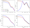 |
Fig. B.1 Same as Fig. 4 but for the Lm case (green curves) and for higher resolution simulations with: a smoothing length ϵ = 0.2 (red curves) and ϵ = 0.1 (blue curves). We remark that decreasing the smoothing length impacts the innermost regions (x < 0.1RH) leaving unchanged the outer part of the Hill sphere. |
References
- Aoyama, Y., Ikoma, M., & Tanigawa, T. 2018, ApJ, 866, 84 [NASA ADS] [CrossRef] [Google Scholar]
- Ayliffe, B. A., & Bate, M. R. 2009, MNRAS, 397, 657 [Google Scholar]
- Bae, J., Zhu, Z., Baruteau, C., et al. 2019, ApJ, 884, L41 [NASA ADS] [CrossRef] [Google Scholar]
- Bai, X.-N. 2017, ApJ, 845, 75 [NASA ADS] [CrossRef] [Google Scholar]
- Bate, M. R., Lubow, S. H., Ogilvie, G. I., & Miller, K. A. 2003, MNRAS, 341, 213 [NASA ADS] [CrossRef] [Google Scholar]
- Bell, K. R., & Lin, D. N. C. 1994, ApJ, 427, 987 [NASA ADS] [CrossRef] [Google Scholar]
- Benisty, M., Bae, J., Facchini, S., et al. 2021, ApJ, 916, L2 [NASA ADS] [CrossRef] [Google Scholar]
- Béthune, W., & Rafikov, R. R. 2019, MNRAS, 488, 2365 [Google Scholar]
- Béthune, W., Lesur, G., & Ferreira, J. 2017, A&A, 600, A75 [NASA ADS] [CrossRef] [EDP Sciences] [Google Scholar]
- Bitsch, B., & Kley, W. 2010, A&A, 523, A30 [NASA ADS] [CrossRef] [EDP Sciences] [Google Scholar]
- Bitsch, B., Crida, A., Morbidelli, A., Kley, W., & Dobbs-Dixon, I. 2013, A&A, 549, A124 [NASA ADS] [CrossRef] [EDP Sciences] [Google Scholar]
- Bitsch, B., Morbidelli, E., L., & Crida, A. 2014, A&A, 564, A135 [NASA ADS] [CrossRef] [EDP Sciences] [Google Scholar]
- Christiaens, V., Cantalloube, F., Casassus, S., et al. 2019, ApJ, 877, L33 [Google Scholar]
- Commerçon, B., Teyssier, R., Audit, E., Hennebelle, P., & Chabrier, G. 2011, A&A, 529, A35 [NASA ADS] [CrossRef] [EDP Sciences] [Google Scholar]
- Cridland, A. J., Facchini, S., van Dishoeck, E. F., & Benisty, M. 2023, A&A, 674, A211 [NASA ADS] [CrossRef] [EDP Sciences] [Google Scholar]
- Cridland, A. J., Benisty, M., & Lega, E. 2024, A&A, submitted [Google Scholar]
- D’Angelo, G., Henning, T., & Kley, W. 2002, A&A, 385, 647 [CrossRef] [EDP Sciences] [Google Scholar]
- D’Angelo, G., Kley, W., & Henning, T. 2003, ApJ, 586, 540 [Google Scholar]
- de Val-Borro, M., Edgar, R. G., Artymowicz, P., et al. 2006, MNRAS, 370, 529 [Google Scholar]
- Fujii, Y., Gressel, O., Tomida, K., & Ziegler, U. 2019, EPSC-DPS Joint Meeting 2019, 2019, 1408 [Google Scholar]
- Fung, J., Artymowicz, P., & Wu, Y. 2015, ApJ, 811, 101 [Google Scholar]
- Fung, J., Zhu, Z., & Chiang, E. 2019, ApJ, 887, 152 [NASA ADS] [CrossRef] [Google Scholar]
- Haffert, S. Y., Bohn, A. J., de Boer, J., et al. 2019, Nat. Astron., 3, 749 [Google Scholar]
- Hartmann, L., Calvet, N., Gullbring, E., & D’Alessio, P. 1998, ApJ, 495, 385 [Google Scholar]
- Hashimoto, J., Aoyama, Y., Konishi, M., et al. 2020, AJ, 159, 222 [Google Scholar]
- Isella, A., Benisty, M., Teague, R., et al. 2019, ApJ, 879, L25 [Google Scholar]
- Keppler, M., Benisty, M., Müller, A., et al. 2018, A&A, 617, A44 [NASA ADS] [CrossRef] [EDP Sciences] [Google Scholar]
- Klahr, H., & Kley, W. 2006, A&A, 445, 747 [NASA ADS] [CrossRef] [EDP Sciences] [Google Scholar]
- Kley, W., Bitsch, B., & Klahr, H. 2009, A&A, 506, 971 [NASA ADS] [CrossRef] [EDP Sciences] [Google Scholar]
- Krapp, L., Kratter, K. M., Youdin, A. N., et al. 2024, arXiv e-prints [arXiv:2402.14638] [Google Scholar]
- Lambrechts, M., & Lega, E. 2017, A&A, 606, A146 [NASA ADS] [CrossRef] [EDP Sciences] [Google Scholar]
- Lambrechts, M., Lega, E., Nelson, R. P., Crida, A., & Morbidelli, A. 2019, A&A, 630, A82 [NASA ADS] [CrossRef] [EDP Sciences] [Google Scholar]
- Lega, E., Crida, A., Bitsch, B., & Morbidelli, A. 2014, MNRAS, 440, 683 [Google Scholar]
- Lega, E., Morbidelli, A., Bitsch, B., Crida, A., & Szulágyi, J. 2015, MNRAS, 452, 1717 [Google Scholar]
- Levermore, C. D., & Pomraning, G. C. 1981, ApJ, 248, 321 [NASA ADS] [CrossRef] [Google Scholar]
- Machida, M. N., Kokubo, E., Inutsuka, S.-i., & Matsumoto, T. 2008, ApJ, 685, 1220 [NASA ADS] [CrossRef] [Google Scholar]
- Machida, M. N., Kokubo, E., Inutsuka, S.-I., & Matsumoto, T. 2010, MNRAS, 405, 1227 [Google Scholar]
- Manara, C. F., Rosotti, G., Testi, L., et al. 2016, A&A, 591, L3 [NASA ADS] [CrossRef] [EDP Sciences] [Google Scholar]
- Marleau, G.-D., Kuiper, R., Béthune, W., & Mordasini, C. 2023, ApJ, 952, 89 [NASA ADS] [CrossRef] [Google Scholar]
- Masset, F. 2000, A&AS, 141, 165 [NASA ADS] [CrossRef] [EDP Sciences] [Google Scholar]
- Mihalas, D., & Mihalas, B. W. 1984, Foundations of Radiation Hydrodynamics (Massachusetts: Courier Corporation) [Google Scholar]
- Morbidelli, A., Szulágyi, J., Crida, A., et al. 2014, Icarus, 232, 266 [Google Scholar]
- Morbidelli, A., Batygin, K., & Lega, E. 2023, A&A, 675, A75 [NASA ADS] [CrossRef] [EDP Sciences] [Google Scholar]
- Müller, A., Keppler, M., Henning, T., et al. 2018, A&A, 617, L2 [Google Scholar]
- Nelson, R. P., Lega, E., & Morbidelli, A. 2023, A&A, 670, A113 [NASA ADS] [CrossRef] [EDP Sciences] [Google Scholar]
- Pinte, C., Dent, W. R. F., Ménard, F., et al. 2016, ApJ, 816, 25 [Google Scholar]
- Ronnet, T., & Johansen, A. 2020, A&A, 633, A93 [NASA ADS] [CrossRef] [EDP Sciences] [Google Scholar]
- Schulik, M., Johansen, A., Bitsch, B., & Lega, E. 2019, A&A, 632, A118 [NASA ADS] [CrossRef] [EDP Sciences] [Google Scholar]
- Schulik, M., Johansen, A., Bitsch, B., Lega, E., & Lambrechts, M. 2020, A&A, 642, A187 [NASA ADS] [CrossRef] [EDP Sciences] [Google Scholar]
- Stolker, T., Marleau, G. D., Cugno, G., et al. 2020, A&A, 644, A13 [EDP Sciences] [Google Scholar]
- Szulágyi, J., Morbidelli, A., Crida, A., & Masset, F. 2014, ApJ, 782, 65 [CrossRef] [Google Scholar]
- Szulágyi, J., Masset, F., Lega, E., et al. 2016, MNRAS, 460, 2853 [Google Scholar]
- Tanigawa, T., Ohtsuki, K., & Machida, M. N. 2012, ApJ, 747, 47 [NASA ADS] [CrossRef] [Google Scholar]
- Turner, N. J., Fromang, S., Gammie, C., et al. 2014, Transport and Accretion in Planet-Forming Disks (Tucson: University of Arizona Press) [Google Scholar]
- Villenave, M., Stapelfeldt, K. R., Duchêne, G., et al. 2022, ApJ, 930, 11 [NASA ADS] [CrossRef] [Google Scholar]
- Wang, J. J., Ginzburg, S., Ren, B., et al. 2020, AJ, 159, 263 [Google Scholar]
- Wang, J. J., Vigan, A., Lacour, S., et al. 2021, AJ, 161, 148 [Google Scholar]
- Zhou, Y., Bowler, B. P., Wagner, K. R., et al. 2021, AJ, 161, 244 [NASA ADS] [CrossRef] [Google Scholar]
- Zhu, Z., Jiang, Y.-F., Baehr, H., et al. 2021, MNRAS, 508, 453 [NASA ADS] [CrossRef] [Google Scholar]
i.e. the typical disk domain for 3D simulations with embedded planets in the paper
except for the small inner bump in the Lm disk where viscous heating dominates; see Fig, A.1, bottom right
All Tables
All Figures
|
Fig. 1 Radial density profiles (top), azimuthally and vertically averaged temperature (middle), and disk aspect ratio (bottom) profiles for the three models at the end of phase A (left) and C (right). The grey dashed lines indicate the boundary of the Hill sphere and the black dotted line the position of the planet. The density of the Lm and LmLv cases has been multiplied by 10 in order to superpose the density background and appreciate the differences in the gap’s depth and width. We notice that in the LmLv case a large amount of gas is accumulated in a radial domain corresponding to the Hill sphere. This is not gas accumulated around the planet but it is the signature of the libration region around the L4 and L5 Lagrangian points not being depleted yet (a known fact in the case of low-viscosity disks). In the middle panel, the midplane temperature is over-plotted with same colours (dashed) on a slice at the planet’s azimuth φ = 0. The higher resolution associated with the deepening of the potential (decreasing smoothing) results in a huge temperature increase up to [1600, 1100, 600] K in the nominal model, the Lm case, and the LmLv model, respectively. In the bottom panel, we remark that it is only in the nominal case that the formation of the gap modifies the aspect ratio considerably. |
| In the text | |
|
Fig. 2 Vertically integrated density of the simulated nominal disk (simulation N in Table 1) in the high-resolution phase (phase C, see text) with non-uniform grid geometry. We clearly see the spiral arms originating at the planet position (xp, yp) = (5.2, 0) [au], revealing the interaction between the planet and the disk. The disk annulus fully contains the gap and slightly extends over the edges. |
| In the text | |
|
Fig. 3 Parameter details for all three models. Left: midplane density field interpolated in cartesian planeto-centric coordinates(x, y) = (R cos(ϕ), R sin(ϕ)) in units of the Hill radius). The cartesian components (υx, υy) of the midplane velocity field are plotted with arrows. The coloured lines are straightforward (full) and backward (dashed) integration of streamlines obtained with the 2D midplane velocity field. Right: azimuthally averaged density field interpolated in planeto-centric coordinates and represented in |
| In the text | |
|
Fig. 4 Parameter details for all three models. Top-left: radiative diffusion timescale (from Eq. (6)). Top-right: opacity. Bottom-left: volume density. Bottom right: temperature. All the quantities are obtained through averages over spherical shells centred on the planet. |
| In the text | |
|
Fig. 5 3D representation of streamlines with initial conditions on the Hill sphere (see Table 2). The colour bar corresponds to planeto-centric mass flow rate on the Hill surface. The sign is negative for mass inflow and positive for mass outflow. The total integration time is short (about four Jupiter orbits) in order to make this plot clear. The evolution of the same streamlines on a longer integration allows us to follow the dynamics on a projected plane (x/RH, y/RH) and to appreciate the evolution of the distance with respect to the planet in Fig. 6. |
| In the text | |
|
Fig. 6 Projection of the streamlines of Fig. 5 on the planetocentric x − y plane (left). The blue contours give the boundaries of the disk. Gas approaching the Hill sphere can have a rapid transit phase in the horseshoe region and be released in the inner or the outer disk trapped in the planetary system. Vertical evolution of streamline with respect to time (middle). Evolution of the distance with respect to the planet as a function of time (right). The dashed lines correspond to backward integration: in the left panel we see that gas approaching the Hill sphere comes from U-turn motion passing close to the planet from the inner or outer branch of the horseshoe region. |
| In the text | |
|
Fig. 7 Same as Fig. 3, right panels showing a zoom close to the planetary system. Vectors of components |
| In the text | |
|
Fig. 8 Absolute value of the inflow and outflow mass rate as a function of z on the Hill sphere. In the Lm and LmLv cases the mass inflow is larger than the mass outflow except very close to the midplane which appears decreating. Instead, in the N case, the Hill sphere is accreting up to z = 0.2[RH] and for z > 0.7[RH]. In all the models, the contribution to the total mass flow in the Hill sphere becomes negligible at z > 0.8[RH]. |
| In the text | |
|
Fig. 9 Accretion rate as a function of the distance to the planet in the Hill sphere computed interpolating the time series of the mass contained in a sphere of radius R over 9 planet’s orbital periods (see text). For each case, we report the rate of inflow (circles) and the accretion rate on the Hill sphere (triangle), as computed on a snapshot at five orbital periods (see Table 3). |
| In the text | |
|
Fig. A.1 Midplane temperature (top) and disks’ aspect ratio (bottom) as a function of radial distance from the host star for 2D simulations for the nominal and Lm cases (left and right, respectively). The red lines include the effect of stellar irradiation. The other simulations have no stellar heating and differ in the boundary temperature, Tb, at disk’s surface. The value of Tb that allows us to recover the profile of the stellar irradiated disk is used for 3D simulations of in the rest of the paper. Horizontal dotted lines in the top plots correspond to the values of Tb in the simulations. The vertical black dotted line marks the position of a Jupiter-mass planet in the paper. |
| In the text | |
|
Fig. B.1 Same as Fig. 4 but for the Lm case (green curves) and for higher resolution simulations with: a smoothing length ϵ = 0.2 (red curves) and ϵ = 0.1 (blue curves). We remark that decreasing the smoothing length impacts the innermost regions (x < 0.1RH) leaving unchanged the outer part of the Hill sphere. |
| In the text | |
Current usage metrics show cumulative count of Article Views (full-text article views including HTML views, PDF and ePub downloads, according to the available data) and Abstracts Views on Vision4Press platform.
Data correspond to usage on the plateform after 2015. The current usage metrics is available 48-96 hours after online publication and is updated daily on week days.
Initial download of the metrics may take a while.