| Issue |
A&A
Volume 693, January 2025
|
|
|---|---|---|
| Article Number | A86 | |
| Number of page(s) | 20 | |
| Section | Planets, planetary systems, and small bodies | |
| DOI | https://doi.org/10.1051/0004-6361/202451140 | |
| Published online | 03 January 2025 | |
Gas dynamics around a Jupiter-mass planet
II. Chemical evolution of circumplanetary material
1
Université Côte d’Azur, Observatoire de la Côte d’Azur, CNRS, Laboratoire Lagrange,
96 Bd. de l’Observatoire,
06300
Nice,
France
2
Univ. Grenoble Alpes, CNRS, IPAG,
414 Rue de la Piscine,
38000
Grenoble,
France
3
Universitäts-Sternwarte München, Ludwig-Maximilians-Universität,
Scheinerstr. 1,
81679
München,
Germany
4
Max-Planck Institute for Astronomy (MPIA),
Königstuhl 17,
69117
Heidelberg,
Germany
★ Corresponding author; A.Cridland@lmu.de
Received:
17
June
2024
Accepted:
25
November
2024
The link between the chemistry of the protoplanetary disk and the properties of the resulting planets have long been a subject of interest in the effort to understand planet formation. These connections have generally been made between mature planets and young protoplanetary disks through the carbon-to-oxygen (C/O) ratio. In a rare number of systems, young protoplanets have been found within their natal protoplanetary disks. These systems offer a unique opportunity to directly study the delivery of gas from the protoplanetary disk to the planet. In this work we post-process 3D numerical simulations of an embedded Jupiter-mass planet in its protoplanetary disk to explore the chemical evolution of gas as it flows from the disk to the planet. The relevant dust to this chemical evolution is assumed to be small co-moving grains with a reduced dust-to-gas ratio indicative of the upper atmosphere of a protoplanetary disk. We find that as the gas enters deep into the planet’s gravitational well, it warms significantly (up to ~800 K), releasing all of the volatile content from the ice phase. This change in phase can influence our understanding of the delivery of volatile species to the atmospheres of giant planets. The primary carbon, oxygen, and sulphur carrying ices (CO2, H2O, and H2S) are released into the gas phase and along with the warm gas temperatures near the embedded planets lead to the production of unique species such as CS, SO, and SO2 compared to the protoplanetary disk. We compute the column densities of SO, SO2, CS, and H2CS in our model and find that their values are consistent with previous observational studies.
Key words: planets and satellites: composition / planets and satellites: formation / planets and satellites: gaseous planets / protoplanetary disks / planet-disk interactions
© The Authors 2025
 Open Access article, published by EDP Sciences, under the terms of the Creative Commons Attribution License (https://creativecommons.org/licenses/by/4.0), which permits unrestricted use, distribution, and reproduction in any medium, provided the original work is properly cited.
This article is published in open access under the Subscribe to Open model. Subscribe to A&A to support open access publication.
1 Introduction
The gravity sculpted gap in the protoplanetary disk (PPD) gas and dust opens in the final stages of a giant planet’s growth. In this stage, the planet has become sufficiently massive that its gravitational influence exceeds the disk viscosity at the midplane, clearing away the co-orbiting material. Gas flows from the PPD towards the embedded protoplanet through the first and second Lagrange points, and from heights above the midplane (the so-called meridional flows, Morbidelli et al. 2014; Szulágyi et al. 2016).
There is a general expectation that this late-stage gas flow will collect into a circumplanetary disk (CPD) because of angular momentum conservation and analogies to star formation. Further evidence of the co-planar Galilean moons of Jupiter suggest that they formed in an analogous way to the rest of the planets around our Sun (i.e. in a disk-like structure around Jupiter, Canup & Ward 2006, 2009). Observing these CPDs (or any circumplanetary material in general) has been primarily attempted through dust emission observation and remains a challenging endeavour due to the possible contamination from surrounding PPD material. As such there are only a few observational works that suggest the presence of a CPD, around the PDS70 protoplanets (Wolff et al. 2017; Christiaens et al. 2019; Stolker et al. 2020; Wang et al. 2020; Benisty et al. 2021; Choksi & Chiang 2024).
Hydrodynamic simulations of this late stage of planet formation have demonstrated that CPDs can form around embedded planets, but require a sufficient level of cooling in order for the gas to settle into a disk-like structure (Ayliffe & Bate 2009; Szulágyi et al. 2014, 2016; Fung et al. 2019; Marleau et al. 2023). In accompanying work, Lega et al. (2024) (hereafter Paper 1) explored the gas flow around an embedded Jupiter-mass planet to characterise the properties of the gas as it passes from the PPD into the gravitational influence of the planet. In the Nominal case, using the minimum mass solar nebula (MMSN) gas densities at a distance of 5.2 AU, the gas is accreted into the planet’s Hill sphere and cools too slowly to form a CPD, and instead remains in a spherically symmetric cloud around the planet. If the surrounding gas density and/or the gas viscosity is reduced, the resulting gas accretion flux allows the gas to cool sufficiently to form a CPD or a rotating structure that is partially supported by pressure that for simplicity we also call a CPD. In this work we consider the simulation results of Paper 1, and explore the chemical evolution of the gas as it moves from the PPD into the CPD.
The primary goal of this work is to understand the chemical environment of the gas surrounding a young proto-planet. This helps to understand two general science questions: (1) how the chemical complexity of the protoplanetary disk gas and dust is imprinted onto the growing planet, and (2) whether there are unique molecular species that make good tracers of circumplanetary material, and that perhaps offer a unique way of detecting CPDs. We posit that the gas entering into the planet’s gravitational influence from the PPD undergoes sufficient chemical processing in the hotter denser environment of the planet’s gravitational well, allowing it to evolve towards a different chemical state than is seen in the PPD. This difference may cause the rate of accretion of different volatile species to change relative to simpler approaches (e.g. in Cridland et al. 2020), and may cause some molecules to appear much brighter in the CPD than in the PPD, enabling a reliable detection method.
Gas line observations have long been used to study the physical and chemical properties of the interstellar medium (ISM) due to their sensitivity to the local properties of the gas and ice (Zuckerman et al. 1976; Draine 1978; Kaufman & Neufeld 1996; Bergin & Snell 2002; van Dishoeck et al. 2021). As we show below, the circumplanetary material presents a significant increase in gas temperature compared to the surrounding PPD, which should drive high-temperature chemistry. We expect that these higher temperatures frees frozen species, particularly water, which further drives oxidising reactions, due to the freed OH radical. For this reason we may expect that the gas around a growing planet has a lower carbon-to-oxygen ratio (C/O) than the gas in the PPD. Jiang et al. (2023) have recently argued the opposite effect of a forming planet, focusing mainly on the release of frozen CH4 due to heating at a distance of a Hill radius from the planet. Here we resolve deeper into the planet’s gravitational well, thus reaching high enough temperatures to release all of the ice budget into the gas. The ice tends to be oxygen rich as its main constituent is H2O (see e.g. Walsh et al. 2015; Cridland et al. 2019a; van Dishoeck et al. 2021; McClure et al. 2023).
The paper is structured as follows. In Sect. 2 we outline the methods used in this work, including the relevant details of Paper 1. In Sect. 3 we present our main results of combining the numerical work of Paper 1 with the chemical model presented here. In Sect. 4 we discuss the relevance of this work and make a comparison with a model of the PDS 70 system. Our conclusions are presented in Sect. 5.
2 Methods
In this follow up work, we post-process the numerical results of Paper 1 using the ALCHEMIST1 (Semenov et al. 2010; Semenov 2017) zero dimensional astrochemistry solver to compute the chemical evolution of gas as it moves along streamlines from the PPD into the gravitational influence of the embedded planet.
2.1 Hydrodynamics simulations
In Paper 1 we explored different outcomes for the distribution of the accreted gas around the embedded planet. Table 1 summarises the parameters of each model considered. The physical link between accretion rate and the gas distribution is through the gas cooling efficiency. For higher accretion rates (the so-called nominal model in Table 1) the gas is not able to cool quickly enough to settle into a rotationally supported disk. Instead, it remains in a pressure supported, spherically symmetric, and hot (~600–1000 K) envelope. Reducing the initial surface density of the PPD at the location of the planet (LowMass model) and/or reducing the viscosity of the gas (LowMassLowVis) results in a sufficiently low accretion rate such that the gas could cool enough for a CPD to form (see also Krapp et al. (2024) for a detailed thermodynamical criterion of CPDs formation).
In this paper, we will primarily focus on the LowMass model from Paper 1, as it produced a CPD around the planet by reducing the surrounding PPD density by a factor of 10. Physically, this reduction is consistent with an older disk that has accreted a significant amount of its mass onto the host star and/or into building giant planets. We discuss the implication of this timing in a later section. Here we will briefly outline the relevant information of the numerical setup and streamline calculation, see Paper 1 for further details. We then outline the chemical setup with its primary assumptions, and outline our analysis techniques.
A common definition that we will use throughout this work is the planet’s Hill radius. The Hill radius represents the size of a sphere centred on any gravitating secondary body within which the gravitational influence of the secondary exceeds that of the primary. In our case, the relevant Hill sphere is that of the embedded planet and its radius is defined as
 (1)
(1)
where ap and Mp is the semi-major axis of the planet’s orbit and mass of the planet respectively, and M* is the mass of the host star. Our general numerical setup, presented in Paper 1, simulates a Jupiter mass planet orbiting at 5.2 AU from the Sun, such that the relevant parameters are ap = 5.2 AU, Mp = 0.000954 M⊙, and M* = M⊙, where M⊙ is the solar mass. As such, the Hill sphere of the embedded planet has a size of RHill = 0.355 AU.
Simulation parameters from Paper 1.
2.1.1 Numerical setup and streamlines
Paper 1 computes the 3D flow of gas in the PPD around an embedded, Jupiter-mass planet, using the fargOCA code (Lega et al. 2014) with a specific grid’s implementation for the study of details in a planet’s Hill sphere introduced in Lambrechts & Lega (2017); Lambrechts et al. (2019). The simulation domain is a full annulus extending from 3 to 7 AU and one hemisphere of the disk. The boundary conditions for the height, azimuthal, and radius are reflective, mirror, and evanescent boundaries respectively. The reference fields for the evanescent boundaries are based on the results of two dimensional, axi-symmetric simulations that reach thermal equilibrium in order to minimise wave reflections (de Val-Borro et al. 2006). The dust is not evolved and a constant dust-to-gas ratio of 0.01, is assumed in order to compute the disk’s opacity. See Paper 1 for further details.
We show an example of the gas distribution from the Low- Mass model of Paper 1 in Figure 1. The figure shows the column density (integrated up the z-axis) of the gas over the entire computation range (left panel) as well as locally to the embedded planet (right panel). The planet cuts a deep gap, with a reduction in gas density of between a factor of 10–100 relative to the surrounding PPD gas. Both the gas flow geometry and the gap are common among all of the simulations shown in Paper 1, however the exact reduction in gas density and the shape of the gap depend on the simulated viscosity and starting density (see Paper 1).
The data that we present in this paper concern a state in which the gas flow has reached a quasi-steady state, where the velocity field does not vary significantly from one timestep to the next. In addition we have shown in Paper 1 that the energy budget of the gas near the planet evolves over timescales of thousands of orbits, implying that the temperature structure also reaches a quasi-steady state. For these reasons, and with the intention to draw streamlines through the velocity field on which we compute our chemical evolution, we take a single snapshot of the simulation to represent the physical structure of gas around the planet. The velocity field is thus kept static during the streamline integration, and the chemistry is computed on the streamline as it evolves from the PPD towards the embedded planet. Paper 1 shows multiple examples of streamlines and discusses some of their general properties. In the streamlines we assume that the dust is co-moving with the gas at a dust-to-gas ratio of 10−4 , we thus assume the chemically relevant dust are composed of small grains. This is discussed in more detail in the following section.
For a better understanding of the global properties of CPDs from a finite set of streamlines, we first characterise the streamlines into a set of ‘families’. These families are classified by the amount of time that the streamlines spend within the CPD relative to total time of the integration, a quantity that is relevant for our chemical study. Specifically, this residence time is computed by taking the difference of t0 , the time when the streamline first enters within r ≤ 0.4 RHill (i.e. in the region where gas is potentially bounded to the planet as found in Paper 1) and tf when the streamline leaves the Hill sphere of the planet. If the streamline never leaves the planet’s Hill sphere, then tf is set to the total integration time tT . With that, the residence time is defined as
 (2)
(2)
The residence time is normalised such that the time between the beginning of the simulation and the point when the streamline first crosses within 0.4 RHill of the embedded planet is ignored.
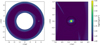 |
Fig. 1 Example of the output from fargOCA, as seen in Paper 1. The figure axes are in units of AU, while the colour range shows the surface density of the gas. The black circle shows the extent of the planet’s Hill radius. |
2.1.2 Treatment of dust
There is no dust included in the simulations of Paper 1, however a constant dust-to-gas ratio is assumed in order to compute dust opacity. Dust plays a very important role in setting the chemical state of the protoplanetary disk. Physically it impacts the thermal balance of the gas by acting as both a strong opacity source to incoming radiation, as well as the primary cooling source. Chemically, dust grains provide the freeze-out site for volatile molecular species when the gas and dust temperatures are sufficient cold, and their surface acts as a catalyst for some chemical reactions.
For the purpose of our chemical calculation we assume that the disk is sufficiently old (given that it contains an embedded giant planet) so that most of the dust mass has grown and settled to the midplane of the protoplanetary disk. Thus the majority of the dust mass will be decoupled from the gas flow and be less important to further chemical evolution as the gas flows from the PPD towards the embedded planet. In the chemical calculations that we will discuss below, we assume that the (chemically) relevant dust grains are strictly small, and dynamically coupled to the gas. From this assumption, the dust density is proportional to the gas density, with a constant (in both space and time) dust- to-gas mass ratio of 10−4. This low ratio, 100 times smaller than is seen in the ISM, is typical for the small grain population in dynamic dust evolution models that include growth and fragmentation in steady state (Dullemond & Dominik 2005; Birnstiel et al. 2010). This low ratio is often observed in the upper atmospheres of protoplanetary disks after the majority of the dust mass has settled (D’Alessio et al. 2006; Meijerink et al. 2009; Bruderer 2013; Bosman et al. 2018).
While the small dust grains make up a very small proportion of the dust mass in the disk, their total number dominate over the large grains (based on the MRN distribution, Mathis et al. 1977). Through this one can find that the small grain population dominates the total dust surface area in the disk and is thus the most important population of grains when it comes to chemical evolution.
2.2 Chemical model
2.2.1 Physical setup
We use the zero dimensional, time dependent astrochemistry code ALCHEMIC (Semenov et al. 2010; Semenov 2017) to solve the chemical evolution of the gas. For each position along the streamline for which we compute chemistry, we extract the temperature and volume density of the gas from the simulation grid of Paper 1 using the REGULARGRIDINTERPOLATOR package of SCIPY after interpolating the temperature and density values from the irregular grid produced by fargOCA onto a regular cartesian grid using the INTERPOLATE package of SCIPY. The interpolation is done linearly.
At each point along the streamline the column density of hydrogen gas is computed towards both the host star as well as vertically upwards from the midplane. This is done in order to compute the relative importance of high energy photons coming from both the host star and from the surrounding ISM. We assume that the host star is a standard T Tauri star with a standard UV field and X-ray luminosity of 1031 erg/s. We find, however that the column density towards the host star implies very a large extinction (Aυ ~ 104) after using a relation between the H2 column density and optical extinction observed by Güver & Özel (2009). On the other hand the minimum vertical extinction is of the order of Aυ ~ 4–10 so that the ISM UV field is important for the chemical evolution. For this we use the UV radiation field of Draine (1978) with the extensions made by van Dishoeck & Black (1982), and assume G0 = 1 at the top of the disk.
We follow the gas as it moves along streamlines from a chosen initial condition. We assume that the gas and dust in the streamline does not interact with the surrounding material, however its temperature and density evolves as the streamline moves through the simulation domain. In this way we ignore diffusion and mixing with the surrounding gas but include possible changes in chemical properties due to changes in the freeze out, desorption, and chemical reaction rates due to changes in gas density and temperature. We assume that the gas velocity field is static over the whole integration time, about 80 orbits in total. From a single initial position, chosen near the planet’s Hill sphere, we integrate the streamline in both the forward (in time) direction as well as the backward direction.
As the streamline evolves forward in time it moves farther into the gravitational potential of the embedded planet, heating up as it does so. A subset of streamlines will pass close to the embedded planet but will not be capture by its gravitational potential and instead will return into the protoplanetary disk. A second group will move into orbit around the embedded planet, representing the formed CPD. We explore the difference between these groups below. The backward integration evolves the streamline away from the embedded planet farther into the protoplanetary disk. There, the streamline encounters features of the disk such as the edge of the planet gap and the spiral arms induced by the embedded planet (see Figure 1) where the density and temperature change slightly compared to the background gas distribution of the protoplane- tary disk (see also Paper 1 for a detailed description of streamline behaviour).
2.2.2 Chemical network
The ALCHEMIC code is equipped with the osu_03_2008 rate file and chemical network with extensions based on the Kinetic Database for Astrochemistry (KIDA, Wakelam et al. 2012). The network includes 6065 chemical reactions of 655 molecular and atomic species. The network includes primarily two-body gas phase reactions such as ion-molecule and neutral-neutral interactions, cosmic ray ionisation and dissociation, gas-grain interactions including neutral and ion absorption as well as thermal-, photo-, and cosmic ray driven-desorption. Finally, the network includes dust grain surface reactions which allow absorbed species to move along the grain lattice and react with other species. The network was featured in Semenov et al. (2018), see that work for more detail.
For the main results of this work we use the network that accompanied ALCHEMIC for computing the chemical evolution of the gas as it moves through the streamline from the PPD to the CPD. Later we will compare our results to separate chemical models of the PDS 70 protoplanetary disk presented in Cridland et al. (2023). These models were run using the DALI thermochemical code (Bruderer et al. 2012; Bruderer 2013) using the chemical network of Miotello et al. (2019) which is based on Visser et al. (2018). This network is largely based on the osu_03_2008 network, but has been optimised to compute C, O, and N chemistry more (computationally) efficient, meaning that some chemical species - such as sulphur - have only limited reactions in the network. We will discuss this later in the paper.
Initial abundances, relative to the total number of hydrogen atoms  .
.
2.2.3 Chemical evolution
The chemical evolution proceeds as follows: the initial temperature and density of the gas is set at the final position of the backward integrating streamline (the coloured triangles in Figure 2). The chemistry at this position is initialised with the abundances shown in Table 2 and integrated for 1 million years (Myr) so that the chemical state of the gas clump reaches a steady state before we allow it to begin moving through the disk. Waiting for 1 Myr to pass is meant to replicate the fact that the protoplanetary disk is at least this old by the time the giant planet has reached the evolutionary phase in which we have initialised the hydrodynamic simulation. The initial Myr also allows the elemental initial conditions time to evolve towards abundant molecular species such as H2O, CO, CO2, and H2S that are relevant in PPDs.
After 1 Myr of evolution we ‘release’ the clump and follow its evolution across the velocity field, we consider t = 0 as the point where the clump is released. The timestep dt of the streamline evolution is set to  , or about a sixth of an orbital period. For a given t ≥ 0 the physical properties of the gas are interpolated as described above for the position along the streamline at t. The chemistry is then integrated to a time of t + dt with a constant temperature and density. The temperature and density are then updated to their interpolated value for a position at time t + dt along the streamline before the chemical evolution is continued.
To facilitate the above algorithm we slightly modified the ALCHEMIC code so that the resulting chemical state computed at one timestep is used as the initial condition for the next timestep. The coupled evolution of the disk chemistry and the physical properties of the disk is similar to the method of Walsh et al. (2015); Eistrup et al. (2016), and matches the modification made in Cridland et al. (2019b).
2.2.4 Initial elemental abundances
The initial abundances are shown in Table 2, and are used to initialise the first 1 Myr of chemical evolution. The position of the gas when it is being initialised in this way is shown by the coloured triangles in Figure 2. The majority of elements are initialised as atoms, apart from H2 , and evolve to form the molecular species in the PPD. The most abundant molecular species to be produced during this initial 1 Myr of evolution are shown in Figure 3. Eistrup et al. (2018) showed that there are differences in the outcome of chemical calculations depending on whether the system is initialised by elemental or molecular abundances (known as the ‘reset’ and ‘inheritance’ scenarios respectively). For our work, this distinction is less important because the gas flows into regions of the disk that are sufficiently warm to effectively reset much of the chemical evolution that occurred prior.
We derived our initial elemental abundances from Bosman et al. (2021), however we ignore the ‘CO depletion’ that they model which adjusts the available carbon and oxygen to further chemical evolution. This CO depletion is meant to replicate the freeze out of volatiles and settling of dust grains that can remove volatile elements from the molecular layer of protoplan- etary disks (see e.g. Krijt et al. 2020). While we ignore this CO depletion, we include a reduction in the dust-to-gas ratio, assuming that the only chemically relevant dust grains are the smallest ones. We thus possibly overestimating the total number of carbon and oxygen atoms available to the chemical evolution of the gas in the streamlines.
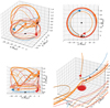 |
Fig. 2 Example of some of the streamlines surrounding the embedded planet. Three types of streamlines are shown: one that misses the CPD completely [(1) blue], one that enters into the region of the CPD for less than an orbit [(2) orange], and one that ends up in the CPD [(3) red]. The solid lines represent forward integration from the initial conditions (black circles), while the dashed lines represent backward integration from the initial conditions. The coloured triangles show the location from which the chemical calculation is initialised. The host star is the black square. The x-axis corresponds to the radial distance along the axis passing through the host star and the embedded planet, centred here on the embedded planet. The y-axis runs perpendicular to the host star–planet axis and the z-axis extends from the midplane to heights above the disk. x > 0 corresponds to a distance farther from the host star than the planet, while y > 0 corresponds to the leading side of the planet’s orbit. |
2.3 Estimating CPD observations
One of our goals in this work is to understand whether there are observational tracers that are uniquely tied to the presence of circumplanetary material. One thing we will find is that the molecular species that are most abundant (i.e. have optically thick emission), such as CO, are poor tracers because differentiating between the PPD and CPD is difficult. On the other hand, optically thin tracers – particularly rarer species that are not abundant in the PPD may turn out to be better tracers of the warm circumplanetary material. As such, their emission will most depend on the total column of a given species along the line of sight. We will estimate the column number density of the molecules that we are interested in, however for simplicity we do not compute the astrochemistry across the whole numerical regime. Instead, we use the positions and chemical properties of the streamline that occupies the CPD to estimate the abundance distributions of molecules around the embedded planet.
The calculation of the column number density proceeds as follows: we focus only on the space centred on the planet and extending out to 1 Hill radius in all directions. For a streamline that orbits in the CPD we have a large set of coordinates (x,y,z) with corresponding temperature, density, and chemical abundance of the gas at those points along the streamline. Over a range of radial distances, r, from the planet we average the abundances of a given molecule over the azimuth amongst the nearest neighbouring coordinates around the circle of radius r. This is done over a large set of heights above the midplane of the CPD and the total column is integrated towards the observer who, we assume, is viewing the disk face on.
In Figure 4 we visualise how the streamlines are used to estimate the CPD column. Here we show a streamline that enters and stays in the CPD (left) as well as the individual points that are computed by the integration routines of Paper 1 (middle). Finally in the right panel we show the set of concentric circles centred around the embedded planet on which we compute the average volume density of a molecule. For 10 separate heights on and above the midplane of the CPD we estimate the average volume density of a given molecule, and integrate along the z-axis. The reported column number density below is over a length scale of 1 Hill radius around the embedded planet, corresponding to a physical lengths scale of 0.355 AU. The results of these calculations are discussed in a later section.
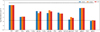 |
Fig. 3 Most abundant initial molecules in their gas and ice phases (prefaced with a ‘g’) for each of the streamline calculations. Apart from molecular hydrogen and helium, the only other gas phase species are CO and CH4 . The other abundant initial species are all in the ice phase because the streamlines each start near the cold midplane of the PPD. The dashed lines ordered from top to bottom give the elemental abundance of oxygen, carbon, and sulphur (oxygen and carbon are overlapping). |
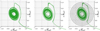 |
Fig. 4 Visualisation of the griding for the column number density calculation, viewed along the z-axis. The left panel shows a zoomed-in image of a streamline that enters into the CPD and remains for the bulk of the integration. The axes show distance relative to the location of the planet, in a rotating reference frame. The middle panel is the same as the left panel, but shows the points along the streamline computed during the integration. The right panel shows each individual point computed along the streamline as well as circles on which we compute the average volume number density of a given molecule at a given r and z in cylindrical coordinates. |
3 Results
3.1 CPD streamline properties
To understand the chemical changes in the gas caused by the local heating in the CPD, we select a subset of streamlines, with different orbital history and study the temporal evolution of the gas as it passes into CPD and any lasting effects as the gas leaves the CPD. Most of our streamlines are initialised near the embedded planet, above the midplane (black circles in Figure 2). Some of these streamlines thus represent gas flow that is commonly called meridional flow. A common evolutionary trend in our numerical simulation is that these streamlines enter into the CPD through this meridional flow, and remain in orbit around the embedded planet. There are a few streamlines that approach near (<0.4 RHill) the embedded planet, but soon after exits the CPD from either the first or second Lagrange point. Gas exiting via the first Lagrange point then co-orbits with the planet at an orbital radius slightly smaller than the planet’s orbital radius while gas exiting the second Lagrange point co-orbits at a slightly larger radius.
To better generalise the chemical properties of the CPD we categorise streamlines into 3 families. Each family is characterised by the amount of time spent in the vicinity of the embedded planet as defined in Eq. (2). As shown in Paper 1, in the LowMass case, the hot inner envelope extends up to 0.2–0.3 Hill radii while orbits captured in the CPD structure have distances from the planet in the interval 0.3 – 0.4 RH. The residence time (tR) measures the amount of time that passes between the gas passing inward of 0.4 RHill from the embedded planet and the gas passing a distance of 1 RHill from the planet. The limiting distance of 0.4 RHill comes from Paper 1, since gas can be bounded to the planet below this distance. Based on these residence times the three families are named as follows:
missed: tR = 0; a streamline that never approaches the embedded planet closer than 0.4 RHill, blue line in Figure 2.
escape: 0 < tR ≤ 0.9; a streamline that approaches within 0.4 RHill but does not end up gravitationally bound to the embedded planet, orange line in Figure 2.
cpd: tR > 0.9; a streamline that falls from the PPD and remains bound in the CPD for the remainder of the simulation, red line in Figure 2.
In Figure 5 we show a series of initial conditions selected on the shell centred on the embedded planet with radii spanning between 0.9 and 1 RHill. Each coloured point on the figure represents a separate initial condition in the streamline calculation and the colour denotes the residence time (as defined above) for each streamline. On the shell of radius of 1 RHill there are small windows of very low residence times distributed between regions of very high residence time streamlines. Figure 6 shows the family representation of Figure 5, where each coloured point represents the initial conditions sorted into each family. The plot shows the set of initial conditions along the central star - planet axis (i.e. the planet is located at the origin of the plot). In this arrangement no streamline initial conditions are found to result in escaping streamlines, which require very particular trajectories.
As a way of assessing the overall importance of each family to the global picture we compute the total gas flux entering into the CPD through each family. On a spherical shell of radius 1 RHill we compute the evolution of a large (10 000) set of streamlines and their associated residence times. The fractional contribution to the total flux through the sphere of 1 Hill radius of each of the streamline families are: (1) missed: 46.0%, (2) escape: 1.0%, and (3) cpd: 53.0%. From this we see that for the flux of gas that crosses 1 RHill from the embedded planet, nearly half of the gas never approaches near the CPD, while just over 50% enters the CPD from 1 RHill . Another tiny fraction of gas enters the region near the embedded planet for a short amount of time before returning to the PPD.
To act as representatives for their family we select one streamline each with initial conditions near the axis connecting the host star and planet, and at a vertical height near 1 RHill. The initial positions of each test streamline is shown in Table 3. In the first column of Figure 7 shows the temperature evolution for the selected streamlines for each family as a function of time. The small, early fluctuations represent the time when the streams are evolving in the protoplanetary disk, while the large fluctuations (up to 800 K) represent the streamlines closest approach to the embedded planet, where their gravitational potential energy is converted to heat. The streamlines that are caught in the CPD enter closest to the embedded planet before slowing moving outwards to lower temperatures. Their orbits appear to be eccentric because of the temperature fluctuations. The two streamlines that enter the CPD (including the escaping one) do so at nearly the same time (~40 orbits) because their forward (and backward) integration begin at a point just prior to the gas entering the CPD. So evolution prior to 40 orbits is represented by the backward integration, while the evolution after 40 orbits is computed by the forward integration. For completeness we show the evolution of the gas density, which plays an important role in the gas chemistry, in Figure A.1.
As an alternative view, the second column of Figure 7 shows the evolution of the temperature with respect to the streamlines’ distance to the embedded planet. The highest temperatures occur when the gas passes by its closest approach to the planet, when it is deepest in the planet’s gravitational well, these closest approaches (rmin) are shown in Table 3. The maximum temperature that each streamline reaches is directly related to the closet approach of the gas. Far from the planet, the gas fluctuates in temperature between ∼38 and ∼44 K as it orbits in the PPD.
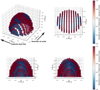 |
Fig. 5 Map of the residence times for a set of initial conditions beginning at a radial distance of 1 RHill from the embedded planet. Each point represents an individual initial condition for the streamline (forward) integration and is colour-coded according to the residence time relative to the difference between the total integration time and the time that the streamline entered into the CPD. The x-axis corresponds to the radial distance along the axis passing through the host star and the embedded planet, centred here on the embedded planet. The y-axis runs perpendicular to the host star-planet axis. The z-axis extends from the midplane to heights above the disk. x > 0 corresponds to a distance farther from the host star than the planet, while y > 0 corresponds to the leading side of the planet’s orbit. Each panel represents the same calculation, but shows different rotations in cartesian space. The bottom left panel represents strictly trailing side initial conditions (y < 0), while the bottom right panel shows the leading side initial conditions (y > 0). |
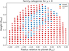 |
Fig. 6 Families: missed (blue), escape (orange), and CPD (red) for the same set of initial conditions as in Fig. 5 and y > 0. In this particular configuration no escape initial conditions can be seen. The radius relative to the planet has the same definition as the x-axis in Fig. 5. |
Properties of the three streamlines in the LowMass model and one from the Nominal model from Paper 1.
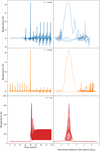 |
Fig. 7 Temperature evolution for test streamlines. The first column shows the temperature as a function of time in orbits of the embedded planet. The second column shows the same temperature evolution of the streamlines as a function of distance from the planet. The streamlines that enter the CPD first do so at around the same time (~40 orbits) because their forward integration is started just before they enter the CPD. In the second row the opacity of the line for t > 40 orbits is reduced as a function of time to better differentiate separate orbits in the CPD. |
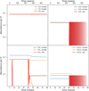 |
Fig. 8 Evolution of the most abundant oxygen-bearing species for the three test streamlines. The solid lines represent the gas phase of each species, while the dashed lines represent the ice species. CH2O2 represents the most abundant organic species in the CPD. We note the change in y-axis range between the top and bottom rows. For water and CH2O2 the opacity of the line for t > 40 orbits is slowly reduced to better see the other lines on the plot. |
3.2 Chemical evolution in the streamlines
3.2.1 Initial molecular abundances at the beginning of the streamline
In Figure 3 we show a collection of the initial molecular abundances of the most abundant species after the first 1 Myr of chemical evolution (i.e. before the gas is released in the streamline). The must abundant gaseous species with elements heavier than helium are CO and CH4 since each of the streamlines begin at temperatures sufficiently high to keep these species in their gas phase. On the other side the gas is sufficiently cold that volatile species such as CO2 and H2O are frozen onto the dust grains. Similarly there are a collection of hydrocarbons, the most abundant of which are C3H2 and C3H4, that are produced on the dust grains through successive hydrogenation of elemental carbon.
Carbon is distributed among many different species, the most abundant of which is CO gas. However there is a significant quantity of carbon distributed among many other species, mainly in the ice phase, primarily hydrocarbons of varying lengths and CO2. Oxygen is mainly found in CO gas, and CO2 and H2O ices, with a very small quantity of organic species such as H2 C3O. Finally, sulphur can be found nearly exclusively in H2S in the ice phase. This follows from the fact that the streamlines originate from the cold midplane of the PPD where H2S can be produced through the hydrogenation of elemental sulphur on the dust grains.
From this initial point we will see that the changing physical properties (density, temperature) of the gas as it travels from the PPD to the CPD drives the molecular inventory of the gas and ice species away from the initial abundances. In the following section, and with their accompanying figures we see that the molecular inventory of the CPD is driven towards molecular species that differ from what was computed in the PPD during the first 1 Myr of chemical evolution.
3.2.2 Streamline chemistry: O-bearing species
In Figure 8 we show the most abundant oxygen-bearing species in the gas of the three test streamlines. We repeat here that the streamlines enter or pass near (in the case of the flyby) the CPD near a time of 40 orbits. At early times (t<40 orbits) the streamlines represent the upper atmosphere of the PPD, where the gas is more strongly irradiated but colder. There, the gas reaches a chemical steady state with abundances shown in Figure 3, and only sees slight changes in abundances as the gas orbits around the PPD. As the gas enters into the gravitational influence of the planet (at t>40 orbits) gas species, such as CO are unaffected. Ice species, on the other hand see a strong change in their abundance due to the rapid increase in gas temperature.
The most abundant ice (water ice) rapidly desorbs as the gas and dust temperatures (which we assume are coupled) increase. As the disk streamline (red line) enters into an orbit around the embedded planet, we see a large fluctuation in the water abundance (top right panel) between the gas and ice phases. This fluctuation is driven by the temperature fluctuation of the gas as the streamline orbits around the embedded planet (see Figure 7). The temperature fluctuation happens to span the freezing temperature of water, and thus it can continually cycles between the two phases in the isolated streamline. In Figure A.2 we focus on a few orbits of time evolution to better visualise the oscillation between the different phases of volatile species.
The bottom left panel shows another abundant ice in the PPD (CO2), which drops its abundance as the streamline enters the CPD, but slightly recovers in the gas phase within the CPD. In PPD chemistry the production of CO2 is largely attributed to the oxidation of CO in the either the gas (at high temperatures) or the ice phase with free OH (Walsh et al. 2015; Eistrup et al. 2018). H2O is thermally dissociated in the gas phase which provides the OH needed to reproduce gaseous CO2 . The free OH can similarly recombine with hydrogen to reproduce H2O, maintaining its high abundance in the CPD. CO2 maintains an abundance ratio relative to H2O of about 4% which is lower than is found in the ice in the PPD. Earlier on in its evolution the disk streamline passes through a warm-spot in the PPD between 0 and 10 orbits that briefly sublimates the CO2 . This warm-spot can be seen in Figure 7 and corresponds to the streamline passing across the spiral wave of the embedded planet.
The bottom right panel shows the most abundant ‘organic’ species that was formed in the CPD, formic acid. Cleeves et al. (2015) model the chemical impact of an accreting proto-planet on the surrounding PPD by computing excess heating on the PPD gas due to the planet’s accretion luminosity. They find that this excess radiation locally heats the PPD and produces an azimuthally asymmetric enhancement in H2CO emission. Instead, in our work we achieve a higher temperatures (few 100s K) deep in the gravitational potential of the embedded planet compared to Cleeves et al. (2015) (60–120 K) which drives our chemical evolution to a more oxidised organic species.
3.2.3 Streamline chemistry: C-bearing species
In Figure 9 we show the dominant carbon-carrying species in the gas. Similar to Figure 8, the left two panels are CO and CO2 , while the other two panels show methane (bottom right) and a larger carbon-chain molecule (top right). In the PPD (t < 40 orbits) we find that methane remains in the gas phase, meaning that the gas is sufficiently warm to exceed the sublimation temperature of methane. This result differs from the physical setup of Jiang et al. (2023), who’s numerical simulations is setup with an embedded planet orbiting father from its host star than we do here. As such their CH4 begins in the ice phase, and its sublimation is the key chemical process that drives important carbon chemistry in their work.
Here we see that carbon chemistry has already produced longer chain hydrocarbons (C3H4, top right panel) in the PPD. These species begin in the ice phase, but are sublimated into the gas phase as the disk streamline enters into the gravitational influence of the embedded planet. Similar to H2O, these long chain hydrocarbons have sublimation temperatures that are within the temperature fluctuation range of the disk streamlines. They thus continue to oscillate between gas and ice phases as the temperature changes.
Methane spends most of its time as a gas and is greatly depleted by the presence of the CPD. In fact most of the methane is produced and maintained in streamlines that spend the most time away from the CPD. CH4 has been observed in proto- planetary disks in the infrared (e.g. Gibb & Horne 2013, using NIRSPEC on Keck), and recent observations in disks with JWST further suggest the presence of CH4 gas emission in one system (Tabone et al. 2023).
3.2.4 Streamline chemistry: S-bearing species
Figure 10 shows the evolution of sulphur-bearing species in the three different families. In these panels, the extent of the y-axes are four orders of magnitudes smaller than the axes of Figures 8 and 9 because sulphur is a less abundant element compared to both carbon and oxygen. While not shown in this figure, we recall that in the PPD the sulphur is primarily in the form of H2S ice (Figure 3). The top two panels show carbon rich sulphur-bearing species while the bottom two panels show oxygen rich ones. For the carbon rich species we see that the PPD starts with a small quantity of H2CS in the ice phase which sublimates once the disk streamlines enters into the CPD (at t>40 orbits). Similarly, all three streamlines show an increase of CS during the closest approach to the planet, but it is sustained for the disk streamline and lost over ∼20 orbits for the two streamlines that stay in the PPD.
Similar to the case of CO2 , when the disk streamline passes through the warm-spot H2CS, CS, and SO are all produced in the gas phase during the briefly increase in temperature. When the streamline moves out of the warm spot the gas cools and all three species freeze out. For the oxygen rich sulphur-bearing species we find that their production and survival depends sensitively on the temperature of the gas. This includes temporary increases in temperature as was mentioned above, but also when the streamlines approach the embedded planet. The escaping streamline (orange) briefly produces both SO and SO2 in the gas phase during its close approach to the planet, but they freeze out and destroyed when the gas cools. The disk streamline also produces both SO and SO2 as it enters into the gravitational potential of the embedded planet. SO2 is only maintained for a short time nearest to the embedded planet where the gas temperatures are the highests. At lower temperatures SO2 can not be maintained and is rapidly depleted. SO, on the other hand is maintained in the CPD over the remainder of the integration time in the CPD. Later in the integration, both the missed and escaped streamline again pass through the spiral wake and breifly for SO and SO2, but again it can not be maintained as the gas temperature returns to its colder temperature.
In the missed and escaped streamlines, the primary sulphur- bearing molecular species ends up being H2S ice – just as it was after the original 1 Myr of chemical evolution in the PPD. The streamline that stays in the CPD, on the other hand, converts nearly all of its H2S into SO, CS, and H2CS. A small quantity of SO2 is also produced but does not remain abundant in the colder regions of the CPD – it only exists in the CPD when gas temperatures exceed ∼500 K. Similar to SO and CS, H2CS has been detected in protoplanetary disks that feature a large dust cavity indicative of an embedded planet (see e.g. Booth et al. 2023a).
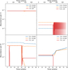 |
Fig. 9 Same as in Fig. 8, but for the most abundant carbon-bearing species. Again, we note the change in y-axis range between the top and bottom rows. For C3H4 the opacity of the line for t > 40 orbits is slowly reduced to better see the other lines on the plot. |
3.3 Streamline chemistry: Nominal model
The Nominal model from Lega et al. (2024) produces a warm gaseous, spherical envelope around the embedded planet rather than a CPD. Similar to the LowMass model, the streamline families can be split between streamlines that spend nearly their whole evolution inside the gravitational influence of the embedded planet, and streamlines that completely miss the gaseous envelope. We select a streamline that spends nearly all of its forward integration time in the gaseous envelope of the embedded planet (see Table 3) and analyse it in a similar manner as was done for the LowMass streamlines.
In Figure 11 we compare the evolution of the gas temperature in the streamline of the nominal model to the disk streamline. Similar to the disk streamline, the streamline in the nominal model begins its forward integration at 40 orbits and slowly spirals closer to the embedded planet, to higher temperatures. In the backward integration (at t < 40) the gas orbits in the corotating region of the embedded planet, and its temperature fluctuates between nearly 200 and ∼20 K. Once it enters into the envelope and spirals close to the embedded planet, its gas temperature fluctuates between 600 and 1000 K.
In Figure 12 we show the evolution of H2O, CO2, SO, and SO2 in the nominal streamline and compare that evolution to the disk streamline. At early times these molecules vary drastically as the gas temperature oscillates in the PPD at t < 40 orbits. This also results in some production of SO in the PPD which oscillates along with the oscillating temperature in the PPD. As the streamline enters into the gaseous envelope surrounding the embedded planet it experiences the high temperatures shown in Figure 11. SO is further enhanced in this high-temperature gas as oxygen carriers such as CO2 are destroyed. The gas stays at these high temperatures so that the SO is eventually destroyed in favour of the more oxygen rich SO2. A small fraction of the freed oxygen reacts with SO to produce SO2 while the rest recombines with available hydrogen to produce H2O. A warm, spherical gas envelope surrounding the embedded planet offers a unique chemical environment compare to the CPD, which generates much less SO2 , and only in the inner regions of the CPD. This difference in chemical behaviour and distribution of sulphur oxides may offer an observational means of differentiating between the difference gas accretion geometries. This would be worth exploring further in the future as it would allow for a more accessible observational means of studying the way that giant planets accrete their gas later in their formation.
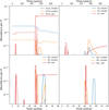 |
Fig. 10 Same as in Fig. 8, but for the relevant sulphur-bearing species. We note here that the axis range on the y-axis has been reduced by about three orders of magnitude compared to Fig. 8, and differs between the top and bottom rows. |
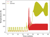 |
Fig. 11 Evolution of the gas temperature of the streamline in the nominal model compared to the temperature evolution of the disk streamline. |
4 Discussion
4.1 Chemical evolution of accreting gas
Cridland et al. (2020) studied the impact on giant planet atmospheric chemistry by the accretion of gas via meridional flow. They sampled the chemical abundances of abundant volatile species (in both the gas and ice phase) in the incoming material at a range of heights above the disk midplane at the gap edge, and assumed that there was no chemical evolution between the gap edge and the accretion of the gas onto the planet. Here we have extended their work and computed the chemical evolution of gas along streamlines from the PPD into the CPD.
Due to the large temperature gradient between the PPD and the CPD all of the frozen volatile species are released into the gas phase very rapidly. This drives the gas to be more oxygen rich (relative to carbon) than it was in the PPD. In addition, since the gas temperature exceeds, for a short time, the sublimation temperature of refractory carbon (∼500 K; Bergin et al. 2015) it is also possible that some of this extra carbon source could be released into the gas. The effect of refractory carbon on the final atmospheric chemistry of giant planet atmosphere has been explored by Cridland et al. (2019a), however for simplicity we have ignored refractory carbon here. It is possible that the extra carbon released from this refractory source could act as a sync for the freed OH what otherwise reacted to produce SO and SO2, possibly reducing their abundance close to the young planet.
Both here and in Cridland et al. (2020) it was assumed that the small (well coupled) dust grains followed the same dynamical evolution as the gas. In Cridland et al. (2020) this implied that volatile species such as H2O could accrete into a giant planet’s atmosphere as ice species frozen on micron-sized dust grains. However, we have seen here that a more accurate expectation is that frozen-out volatiles should be released into the gas as it travels from the PPD, furthermore we might expect that the dust grains will grow while in the CPD (as explored by Drazkowska kowska & Dullemond 2018; Batygin & Morbidelli 2020; Shibaike & Mori 2023, among others), and become decoupled to the gas. This dust growth could, in the future, drive moon formation, but will also lead to less efficient volatile freeze-out as the available surface area per mass of the dust is reduced.
With that said, it is clear from this work that in considering the delivery of important elemental species (C, O, N, and S) to the atmosphere of the growing planet, we may assume that all volatile species (whether they are in the gas or ice phase) will follow the flow of the gas after entering into the CPD. This conclusion requires the gas to reach high enough temperatures (≳100 K) to sublimate all of the volatiles, which was easily reached here but could be more difficult as the mass accretion rate onto the CPD drops and the disk around the planet cools. This could thus imply that older planet-forming systems will generate fewer oxides because their water will remain in the ice phases.
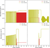 |
Fig. 12 Comparison between a streamline in the nominal model and the LowMass model, using the disk streamline. As before the solid lines show the gas phase, while the dashed lines show the ice phase. |
4.2 Formation and structure of the CPD
Our physical model represents a protoplanetary disk that is depleted in gas density compared to the MMSN by a factor of 10. As previously mentioned this can correspond to a more evolved disk that has accreted a significant amount of its mass either into the host star or into the formation of giant planets. As found in Paper 1, the LowMass model produces a CPD because the gas flux into the planet’s Hill sphere was sufficiently low that it could cool in time to collapse into a rotationally support structure. In the Nominal model the protoplanetary disk was initialised with the standard MMSN, but rather than produce a rotationally supported disk it instead produces a pressure supported spherical envelope around the embedded planet. This result corresponds to the ones found in Klahr & Kley (2006); Szulágyi et al. (2016); Fung et al. (2019); Lambrechts et al. (2019); Krapp et al. (2024) where the gas equation of state was treated in a similar manner to what was done in Paper 1.
In Figure 13 we show a 2D view of the azimuthally averaged mass ratio of the water ice and gas species in the CPD, based on the disk streamline. The grey hatches represent the space around the embedded planet where that streamline does not visit during the simulation. Given the warm nature of the CPD, we find that the gas phase dominates the abundance of volatile species, including when we analyse individual molecules. In our simulated CPD we lack any so-called ‘ice line’, along the midplane of the disk because its temperature is too warm for volatile freeze out there. Higher above the CPD, in a shallower part of the gravitational potential the gas is cooler and water can thus freeze out. Likewise we find that the CO2 ice line exists at an even higher height above the midplane, in a further colder area around the embedded planet (see figure 14).
This could complicate the view that ice lines, particularly the water ice line, play an important role in the formation of the Jovian moons (see e.g. Heller & Pudritz 2015). Alternatively this suggests that moon formation from CPDs could occur later in the planet formation process, at a stage when the CPD is effectively cut off from future gas flow from the PPD. At this later stage, the CPD could cool which would allow for the emergence of the water ice line along the midplane of the CPD. A late stage of moon formation was argued by Canup & Ward (2002), who found that Galilean moon formation was most consistent with mass accretion rates from the PPD to the CPD of 2 × 10⁻⁷ Jupiter masses per year. Over a sphere of radius 1 RHill we find that the mass inflow rate in the LowMass model is 1.8 × 10⁻⁵ Jupiter masses per year, two orders of magnitude higher than predicted by Canup & Ward (2002). Our simulated CPD thus represents an early state of a CPD, where it is too warm and has too large of accretion rate to likely lead to moon formation.
We note here that our model of focus – the LowMass model – represents a state where the gas density of the PPD is already reduced by an order of magnitude relative to the Nominal model (see Table 1 and Paper 1). As previously implied, the LowMass model could represent an older stage of PPD evolution than the PPD initialised in the Nominal model. However, as previously noted, our modeled mass accretion rate into the region of the planet’s gravitational influence is two orders of magnitude higher than was predicted in moon formation studies, which further emphasises the delayed nature of moon formation. This may imply that young systems that have bright, localised SO emission, for instance HD 169142 (Law et al. 2023), do not have ongoing moon formation around their embedded planet, while older systems such as PDS 70 that has very low ongoing mass accretion (as suggested by Haffert et al. 2019) could be actively producing moons around their giant planets.
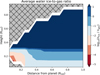 |
Fig. 13 Aziumthally averaged H2O ice-to-gas mass ratio of the CPD and material surrounding the embedded planet. The CPD extends to ~0.4 RHill. We based the calculation on the disk streamline, and thus the hatched region shows where the streamline did not visit during the simulation. The traditional ice line, where the abundance of gas and ice species are equal, exists above the disk midplane, suggesting that no ice lines exist in the CPD. |
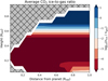 |
Fig. 14 Aziumthally averaged CO2 ice-to-gas mass ratio of the CPD and material surrounding the embedded planet. The traditional ice line, where the abundance of gas and ice species are equal, lies well above the disk midplane, due to the warm nature of the circumplanetary material. |
4.3 Observational tracers of CPDs
Given the recent interest in detecting planets in younger stages of evolution – the so-called proto-planet phase – as well as their presumed circumplanetary material, we explore what chemical tracers may be relevant to detecting CPDs. From Figures 8–10 we saw that many volatile species are in their gas phase in the CPD thanks to the much higher gas temperatures in the CPD (at least ≤200 K) compared to the surrounding PPD. The most abundant molecular species – CO – shows very little variation between being inside and outside of the CPD, and would thus be a poor tracer. This is due to the higher temperature of the protoplanetary disk gas that surrounds the embedded planet, which exceeds the freeze-out temperature of CO.
Other abundant species (i.e. H2O and CO2) are in the ice phase in the PPD – the embedded planet orbits sufficiently far enough away that the gas is colder than their freeze-out temperature. Meanwhile in the CPD the gas temperature exceeds their freeze-out temperature, and they exist mainly in the gas phase – indeed CO2 is first destroyed at the highest CPD temperatures but is then produced in the CPD through the oxidation of CO by OH. H2O is thermally dissociated, producing the needed OH for the aforementioned oxidation reaction, and elemental hydrogen. Because of the high abundance of hydrogen, many of the freed OH react to reproduce H2O. The chemistry in the CPD is not so different from the chemistry in the inner few AU of the PPD and as such the inner disk may turn out to outshine the CPD.
Sulphur-bearing species offer a potential way of differentiating between the CPD and PPD. SO and SO2 are known tracers of high-temperature gas, mainly in astrophysical shocks. Here (see Fig. 10), we see that the gas becomes more abundant in SO when the streamlines orbit in the CPD, and these species are effectively obsolete when the gas is in the colder PPD midplane. A very common molecular carrier of sulphur, H2S remains primarily in the ice phase throughout the evolution of the streamlines, and is rapidly destroyed when the gas temperature exceeds ~200 K. In the CPD the conversion from H2S ice to species such as CS, SO, and SO2 is driven by high-temperature chemistry, and the availability of oxidisers such as OH from the desorption and destruction of H2O ice. There have been a small collection of observations of these heavier sulphur species made in protoplanetary disks. Chemical models have shown that the ratio of CS/SO is very sensitive to the local gas C/O (Semenov et al. 2018), and they have thus been primary targets to chemically characterise protoplanetary disks (Booth et al. 2021; Keyte et al. 2023; Law et al. 2023; Booth et al. 2023a, 2024). Interestingly, all of these observations show azimuthal asymmetries in the emission of sulphur-bearing species and many of these asymmetries have been attributed to the presence of young, embedded, planets. In particularly HD 169142, an SO emission ‘blob’ has been found co-located with the proposed location of a young planet that has been inferred from other observational methods (Law et al. 2023). The possible link between oxidised sulphur species and the presence of embedded proto-planets is an interesting line of research for which we find some evidence here.
4.4 Finding the needle in the haystack
From their high abundance and relative uniqueness, we might expect that CPDs shine brighter in SO and SO2 emission lines than the surrounding gas in the PPD. This is complicated however, by the fact that the warm gas in the upper layers of the PPD will also produce some amount of oxidised sulphur species. In face-on disks, the CPD may represent an asymmetry in the emission structure of SO and SO2 which could help to localise the position of young proto-planets and their circumplanetary material.
At the end of Section 2 we outline our method of estimating the column number density of the CPD from the disk streamline. The column densities implied by our streamline calculation on a length scale of 1 Hill radius provides estimates of 2.0 × 10¹⁴, 7.3 × 10¹⁴, 4.6 × 10¹⁴, and 1.7 × 1017 cm−2 in the CPD for SO, SO2, CS, and H2CS respectively. These represent the total column number densities from the midplane of the CPD up towards the observer assuming that the system is observed face-on. Furthermore this calculation ignores any optical depth effects due to the presence of dust grains. These calculation thus represent the maximum possible column number density that could be inferred observationally.
As a first step in understanding the detectability of CPDs in young stellar systems we turn to the well known PDS 70 system (Keppler et al. 2018; Benisty et al. 2021). Recent sub-mm emission has suggested that PDS 70c has some surrounding circum-planetary material while PDS 70b does not (Benisty et al. 2021). Cridland et al. (2023) explored a chemical model of the PPD around PDS 70 in order to understand the chemical properties of the gas that built the PDS 70b and PDS 70c planets. Their chemical model used the thermo-chemical code DALI (Bruderer et al. 2012; Bruderer 2013) and used the chemical network of Miotello et al. (2019) which focused on carbon chemistry and the production of small chain hydrocarbons, but lacked any sulphur chemistry.
To facilitate a comparison between the gas column densities inferred in the CPD of this model and the gas column densities inferred in the PPD surrounding PDS 70, we recompute the chemistry of the ‘best fit’ physical model of Cridland et al. (2023) using an updated chemical network. This network combines the network used in Cridland et al. (2023) with a set of 330 sulphur-relevant reactions that are included in the osu_03_2008 network. In this way the carbon chemistry, which was the main driver for finding the best fit physical model in Cridland et al. (2023), should remain largely unchanged while the sulphur chemistry of the PDS 70 disk can be newly analysed.
We first check that adding the extra reactions to the network used in Cridland et al. (2023) does not greatly impact the results of that work (see the left panel of Figure 15). In the figure we show a comparison between the two networks (labelled by the elements they include) for different assumed elemental abundances of carbon and oxygen, the sulphur abundance is kept constant at S/H = 1.91 × 10⁻⁸ throughout. In the left panel of Figure 15 we can see that the addition of the sulphur-relevant reactions has not greatly changed the distribution of the C2H column that was primarily used to restrict the physical model of the PDS 70 disk.
An important feature of the PDS 70 disk is that it has a deep gap in the dust and gas which has been carved out by the young PDS 70b and c planets. This gap can be seen in Figure 15 as the drop of about 3–4 orders of magnitude in the C2H column density. Such a deep gap may further simplify the detection of a CPD in molecular emission because the surrounding PPD emission is suppressed by the low column density.
In the middle and right panels of Figure 15 we show the column densities of the SO and SO2 in the full network respectively. We see a similar drop in the column density at the location of the combined planetary gap. In both cases we see an even larger drop in the column density relative to the abundances in the inner and outer disk than was seen in C2H. This could imply an even greater contrast between the PPD and CPD SO2 emission. The column number densities in the CPD are about a factor of 10 larger than the SO and SO2 column of the gas in the outer disk inferred in the PDS 70 models (see the dot-dashed lines in Figure 15). This implies that their emission should be brighter compared to the rest of the PPD.
Recently Rampinelli et al. (2024) report a weak detection of SO emission from the PDS 70 disk in a spacial resolution chemical survey of the disk. The peak emission, however, does not coincide with the positions either PDS 70b nor PDS 70c and instead peaks farther from the host star than the continuum emission ring. The emission non-detection near the PDS 70 proto-planets implies that any circum-planetary material that may be around them is not sufficiently hot to produce SO chemical, nor excite the specific lines observed. Given that PDS 70 is an older system this result is not surprising because the ongoing planetary accretion rate (as inferred from H-alpha emission Haffert et al. 2019) is very low.
For slightly younger systems the picture is more complicated. Recently Booth et al. (2023a) reported the detection of SO emission from the planet-hosting Herbig star HD 100546, while Booth et al. (2023b) report SO emission from the planet-hosting young system HD 169142. In both cases the emission is asymmetric around the disk’s rotation axis and shows signs that the asymmetries are related to the presence of the embedded planets. The column number density of SO is estimated to be 2.1 × 1013 cm−2 over the whole disk in HD 169142 and 4.9 × 1013 cm−2 in the north-east ‘blob’ (Law et al. 2023). This estimate in the ‘blob’, at the position of a suspected planet, is a factor of 4 lower than our estimate from the streamline chemistry. This discrepancy can be easily explained by the presence of dust providing a source of opacity to shield some of the emission from these molecular species.
Nevertheless we expect that the emission of some of these sulphur-bearing species in young systems containing an embedded planet and circumplanetary material will be asymmetric around their rotation axis. This could lead to a separate test of the presence of young protoplanets and CPDs to reinforce other methods.
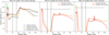 |
Fig. 15 A comparison between the derived column densities of relevant chemical species for a specific chemical model of PDS 70 (Cridland et al. 2023) and the column densities estimated from this work. Left: comparison between the C2H column density values of the different chemical networks mentioned in the text. The networks are Miotello et al. (2019) which include C, H, O, & N (C/H/O/N) and Miotello et al. (2019) + Bruderer (2013) which include C, H, O, N, & S (C/H/O/N/S). We tested that the resulting column density showed minimal change when adding the extra sulphur reactions to the network of Miotello et al. (2019). There is minimal change in the column density for the different networks regardless of the elemental abundance of carbon and oxygen, which we vary between the ISM value (C/O = 0.4) and the abundance inferred for PDS 70 (C/O = 1.01) by Cridland et al. (2023). The dashed lines show the orbital positions of the b and c planets. Middle: same as left panel, but for SO. In the Miotello et al. (2019) network, SO and other more complex sulphur-bearing species are not included. The models shown in the left panel corresponding to that network are thus left out here. The dot-dashed line shows the estimated column density from our chemical model along the streamlines. Right: same as middle panel, but for SO2. |
4.5 Caveats and future prospects
As a first step to understanding the chemical properties of the gas flowing from the PPD to the CPD we have taken a single snapshot of the velocity field to compute our streamlines. We have checked in Paper 1 that the simulation had reached a steady state, however in principle the velocity field may change slightly over a dynamical time. A given streamline may thus shift slightly from its computed trajectory shown here. While this might impact an individual streamline, it does not greatly impact the properties of the gas that control the chemistry – mainly the gas temperature and density – and so shouldn’t change our overall conclusions.
4.5.1 Diffusion
We treat each streamline as an individual packet of gas with small (well coupled) dust grains. We ignore the impact of diffusion between a gas packet and the surrounding gas, which may have an impact on the evolution of the gas as it moves from the PPD to the CPD. In particular this effect may be greatest in the CPD where the temperatures/densities are the highest. Diffusion may mix volatiles species out of the gas packet, decaying the desorption/absorption oscillation that we see in Figure 8 (especially H2O). Removing H2O from the gas packet reduces the production of OH and subsequently may lead to less efficient production of SO in the CPD, leading to a slight reduction in its line emission brightness.
4.5.2 Heating and cooling
We ignore the radiative heating of the forming planet on the gas temperature and high energy photon flux (impacting photodissociation and ionisation). The young planet radiatively heats both the gas and dust in the CPD as well as the gas in the PPD nearby. This has been explored by many past authors (e.g. Heller & Pudritz 2015, explored the impact of accretion heating on the water ice line location in the CPD), in particular the work of Cleeves et al. (2015) who suggest that azimuthal asymmetries in the molecular line emission of some voaltiles should arise from the local accretional heating of the growing planet. Furthermore, the thermal effects within the Hill sphere and the thermal structure of the disk have been explored by Jiang et al. (2023) and Chen et al. (2024) respectively. These effects could change the overall chemical evolution of the gas as it flows, and we leave this to future work.
Along with the radiative flux, the gas can be shock heated as it compacts the accretion planet, its magnetic field, and/or the CPD. We include (see Paper 1) compressional heating, which follows P∇ ⋅ v, due to the converging gas flows. However with finite spacial resolution it is possible that we do not fully resolve the shock front and miss the maximum temperature within the shock. In the shock chemistry model of van Gelder et al. (2021) SO also tends to be more abundant than SO2 at the end of the shock which is similar to our results here. Future work could explore the energetics of the line emission which could depend on the exact temperature structure of the shocking gas.
One common feature of the CPD streamlines is their oscillating temperature as they orbit the embedded planet. It is possible that the cooling rates within the gas parcel are not sufficiently fast to account for the rapid temperature oscillations that are inferred in our method. Using the standard Bell & Lin (1994) opacity dependence on density and temperature, the functional form of the cooling rate from Paper 1 (ρκParT4)2, and the assumption that the gas energy density (e) follows P = (γ – 1)e for an ideal gas with γ = 1.4 we estimate a cooling timescale between 0.1 and 0.2 orbits. The gas streamlines orbit the embedded planet roughly 6 times per orbit of the planet, meaning that their orbital timescale is approximately 0.16 orbits.
With similar timescales, it is unlikely that the gas would be able to cool from ~300 down to ~80 K within a single orbit which would imply that the gas would stay nearer to the higher of the two temperatures during the orbit of the streamline. This may not change our ultimate conclusions because the important chemical processes occur when the temperature is at its highest, when the water is in its gas phase.
4.5.3 High energy photons
Finally, we note that the process of accretion is generally linked to an enhanced UV flux due to shocking gases and high temperatures. We have ignored any extra UV flux from the accreting planet in computing the local radiation field and its effect on the chemical evolution. We note that the temporal evolution of the accreting planet’s luminosity has been modelled in the past (e.g. by Mordasini 2013) and the accretion history of the planet could impact the ongoing chemical evolution of the gas in the CPD. A more thorough investigation over a longer time-frame is needed, including an investigation of the chemical properties of the circumplanetary material when the embedded planet is less massive and thus has a shallower gravitational potential.
5 Conclusion
In this work we post-processed numerical simulations of gas flow around an embedded Jupiter-mass planet. We computed the chemical evolution of the gas as it flows from the PPD into the gravitational influence of the embedded planet. For our selected simulation, the LowMass model of Paper 1, the circumplanetary material is organised into a CPD. There is a significant temperature gradient (nearly 800 K) between the PPD and the warmest regions of the CPD that releases all of the volatile ices from the coupled dust grains into the gas phase. The high temperatures and releases of frozen species result in high-temperature chemistry, which drives the formation of sulphur-bearing species that are otherwise absent in our simulated PPD. We generally find the following:
Abundant volatiles such as H2O, CO2, and H2S are released into the gas phase, making the gas more oxygen and sulphur rich.
CH4 is dissociated in the warm gas around the embedded disk, allowing the production of more long-chain hydrocarbons, which exist in both the gas and ice phases in the CPD.
Both carbon- and oxygen-bearing sulphur species are produced in the warm temperatures around the embedded planet, and are maintained in the gas phase.
The high temperatures of the CPD exclude the existence of any canonical volatile ice lines along the midplane of the CPD. The lack of these lines limits the possibility of moon formation within our modelled CPD.
The possible contrast in column number densities between the CPD and surrounding PPD, SO, SO2, and CS could be used to trace the presence of young embedded proto-planets in their natal PPD by looking for bright azimuthal asymmetries in the emission of those molecules.
The systems that show strong emission in the aforementioned molecules are likely in an intermediate state of formation. Occurring at an age when the surrounding PPD has evolved sufficiently to lower its mass accretion rate by an order of magnitude, but early enough that the CPD has not sufficiently cooled to allow for the production of moons.
Based on the empirical fit of Hartmann et al. (1998), an order of magnitude reduction of mass accretion rate relates to an age of a few million years, while the only confirmed example of protoplanets with an accompanying natal disk (PDS 70) is at least 5 Myr old and has remarkably low mass accretion (Haffert et al. 2019). Our model thus best represents protoplanet-protoplanetary disk systems that are of the order of a few million years in age, at a stage when the circumplanetary material is still quite warm.
Acknowledgements
Thank you to the anonymous referee for their insightful comments which improved the clarity of the manuscript. A.C. and M.B. acknowledges funding from the European Research Council (ERC) under the European Union’s Horizon 2020 research and innovation programme (PROTOPLANETS, grant agreement No. 101002188). Exoplanet studies at the LMU are done as part of the Theoretical Astrophysics of Extrasolar Planets research chair. This project made use of the following software: Astropy (Astropy Collaboration 2022), SciPy (Virtanen et al. 2020), NumPy (van der Walt et al. 2011), and Matplotlib (Hunter 2007).
Appendix A Supplementary figures
A.1 Streamline density evolution
In figure A.1 we show the density evolution of streamlines mainly in the PPD (missed and escape; blue and orange, respectively) and the one that enters into the CPD (disk; red). There is a significant difference in the gas volume density for the disk streamline which alter the steady state sublimation temperature of volatiles by increasing the rate at which the gas can re-collide with the dust grains.
A.2 Chemical evolution zoom-in
In figure A.2 we show a zoomed-in view of the chemistry of the streamlines near where they had their closest approach to the embedded planet, and when the disk streamline (red) enters the CPD. We focus mainly on the first few orbits after the disk streamline enters the CPD where the density (figure A.1 and temperatures (figure 7) are the highest.
There we still see an oscillation between gas (solid) and ice (dashed) phases for these species and as the disk streamline cycles away from the embedded planet, to cooler temperatures the fraction of ice/gas approaches a state where the two phases oscillate perfectly between one and the other. Species with similar production pathways as SO, require OH in the gas phase to be formed also oscillate as the source of OH, H2O vapour oscillates between its gas and ice phase.
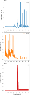 |
Fig. A.1 Density evolution for the three test streamlines in the LowMass model. The disk streamline (red) experiences an increase in gas density by about three orders of magntiude when it enters into the CPD. |
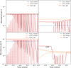 |
Fig. A.2 Zoomed-in view of the chemical evolution of each streamline just after t = 40 orbits, or when the streamlines undergo their closest approach to the embedded planet, and disk streamline enters the CPD. The selected species are the ones that undergo oscillation in the CPD as the streamline orbits in and out of warm CPD regions. |
References
- Astropy Collaboration (Price-Whelan, A. M., et al.) 2022, ApJ, 935, 167 [NASA ADS] [CrossRef] [Google Scholar]
- Ayliffe, B. A., & Bate, M. R. 2009, MNRAS, 397, 657 [Google Scholar]
- Batygin, K., & Morbidelli, A. 2020, ApJ, 894, 143 [NASA ADS] [CrossRef] [Google Scholar]
- Bell, K. R., & Lin, D. N. C. 1994, ApJ, 427, 987 [NASA ADS] [CrossRef] [Google Scholar]
- Benisty, M., Bae, J., Facchini, S., et al. 2021, ApJ, 916, L2 [NASA ADS] [CrossRef] [Google Scholar]
- Bergin, E. A., & Snell, R. L. 2002, ApJ, 581, L105 [NASA ADS] [CrossRef] [Google Scholar]
- Bergin, E. A., Blake, G. A., Ciesla, F., Hirschmann, M. M., & Li, J. 2015, Proc. Natl. Acad. Sci., 112, 8965 [NASA ADS] [CrossRef] [Google Scholar]
- Birnstiel, T., Dullemond, C. P., & Brauer, F. 2010, A&A, 513, A79 [NASA ADS] [CrossRef] [EDP Sciences] [Google Scholar]
- Booth, A. S., van der Marel, N., Leemker, M., van Dishoeck, E. F., & Ohashi, S. 2021, A&A, 651, L6 [NASA ADS] [CrossRef] [EDP Sciences] [Google Scholar]
- Booth, A. S., Ilee, J. D., Walsh, C., et al. 2023a, A&A, 669, A53 [Google Scholar]
- Booth, A. S., Law, C. J., Temmink, M., Leemker, M., & Macías, E. 2023b, A&A, 678, A146 [NASA ADS] [CrossRef] [EDP Sciences] [Google Scholar]
- Booth, A. S., Temmink, M., van Dishoeck, E. F., et al. 2024, AJ, 167, 165 [NASA ADS] [CrossRef] [Google Scholar]
- Bosman, A. D., Walsh, C., & van Dishoeck, E. F. 2018, A&A, 618, A182 [NASA ADS] [CrossRef] [EDP Sciences] [Google Scholar]
- Bosman, A. D., Alarcón, F., Bergin, E. A., et al. 2021, ApJS, 257, 7 [NASA ADS] [CrossRef] [Google Scholar]
- Bruderer, S. 2013, A&A, 559, A46 [NASA ADS] [CrossRef] [EDP Sciences] [Google Scholar]
- Bruderer, S., van Dishoeck, E. F., Doty, S. D., & Herczeg, G. J. 2012, A&A, 541, A91 [NASA ADS] [CrossRef] [EDP Sciences] [Google Scholar]
- Canup, R. M., & Ward, W. R. 2002, AJ, 124, 3404 [Google Scholar]
- Canup, R. M., & Ward, W. R. 2006, Nature, 441, 834 [NASA ADS] [CrossRef] [Google Scholar]
- Canup, R. M., & Ward, W. R. 2009, in Europa, eds. R. T. Pappalardo, W. B. McKinnon, & K. K. Khurana (Tucson: University of Arizona Press), 59 [Google Scholar]
- Chen, K., Kama, M., Pinilla, P., & Keyte, L. 2024, MNRAS, 527, 2049 [Google Scholar]
- Choksi, N., & Chiang, E. 2024, arXiv e-prints [arXiv:2403.10057] [Google Scholar]
- Christiaens, V., Cantalloube, F., Casassus, S., et al. 2019, ApJ, 877, L33 [Google Scholar]
- Cleeves, L. I., Bergin, E. A., Qi, C., Adams, F. C., & Öberg, K. I. 2015, ApJ, 799, 204 [CrossRef] [Google Scholar]
- Cridland, A. J., Eistrup, C., & van Dishoeck, E. F. 2019a, A&A, 627, A127 [Google Scholar]
- Cridland, A. J., van Dishoeck, E. F., Alessi, M., & Pudritz, R. E. 2019b, A&A, 632, A63 [NASA ADS] [CrossRef] [EDP Sciences] [Google Scholar]
- Cridland, A. J., Bosman, A. D., & van Dishoeck, E. F. 2020, A&A, 635, A68 [NASA ADS] [CrossRef] [EDP Sciences] [Google Scholar]
- Cridland, A. J., Facchini, S., van Dishoeck, E. F., & Benisty, M. 2023, A&A, 674, A211 [NASA ADS] [CrossRef] [EDP Sciences] [Google Scholar]
- D’Alessio, P., Calvet, N., Hartmann, L., Franco-Hernández, R., & Servín, H. 2006, ApJ, 638, 314 [Google Scholar]
- de Val-Borro, M., Edgar, R. G., Artymowicz, P., et al. 2006, MNRAS, 370, 529 [Google Scholar]
- Draine, B. T. 1978, ApJS, 36, 595 [Google Scholar]
- Drazkowska, J., & Dullemond, C. P. 2018, A&A, 614, A62 [NASA ADS] [CrossRef] [EDP Sciences] [Google Scholar]
- Dullemond, C. P., & Dominik, C. 2005, A&A, 434, 971 [CrossRef] [EDP Sciences] [Google Scholar]
- Eistrup, C., Walsh, C., & van Dishoeck, E. F. 2016, A&A, 595, A83 [NASA ADS] [CrossRef] [EDP Sciences] [Google Scholar]
- Eistrup, C., Walsh, C., & van Dishoeck, E. F. 2018, A&A, 613, A14 [NASA ADS] [CrossRef] [EDP Sciences] [Google Scholar]
- Fung, J., Zhu, Z., & Chiang, E. 2019, ApJ, 887, 152 [NASA ADS] [CrossRef] [Google Scholar]
- Gibb, E. L., & Horne, D. 2013, ApJ, 776, L28 [NASA ADS] [CrossRef] [Google Scholar]
- Güver, T., & Özel, F. 2009, MNRAS, 400, 2050 [Google Scholar]
- Haffert, S. Y., Bohn, A. J., de Boer, J., et al. 2019, Nat. Astron., 3, 749 [Google Scholar]
- Hartmann, L., Calvet, N., Gullbring, E., & D’Alessio, P. 1998, ApJ, 495, 385 [Google Scholar]
- Heller, R., & Pudritz, R. 2015, ApJ, 806, 181 [NASA ADS] [CrossRef] [Google Scholar]
- Hunter, J. D. 2007, Comput. Sci. Eng., 9, 90 [NASA ADS] [CrossRef] [Google Scholar]
- Jiang, H., Wang, Y., Ormel, C. W., Krijt, S., & Dong, R. 2023, A&A, 678, A33 [NASA ADS] [CrossRef] [EDP Sciences] [Google Scholar]
- Kaufman, M. J., & Neufeld, D. A. 1996, ApJ, 456, 611 [NASA ADS] [CrossRef] [Google Scholar]
- Keppler, M., Benisty, M., Müller, A., et al. 2018, A&A, 617, A44 [NASA ADS] [CrossRef] [EDP Sciences] [Google Scholar]
- Keyte, L., Kama, M., Booth, A. S., et al. 2023, Nat. Astron., 7, 684 [NASA ADS] [CrossRef] [Google Scholar]
- Klahr, H., & Kley, W. 2006, A&A, 445, 747 [NASA ADS] [CrossRef] [EDP Sciences] [Google Scholar]
- Krapp, L., Kratter, K. M., Youdin, A. N., et al. 2024, ApJ, 973, 153 [NASA ADS] [CrossRef] [Google Scholar]
- Krijt, S., Bosman, A. D., Zhang, K., et al. 2020, ApJ, 899, 134 [NASA ADS] [CrossRef] [Google Scholar]
- Lambrechts, M., & Lega, E. 2017, A&A, 606, A146 [NASA ADS] [CrossRef] [EDP Sciences] [Google Scholar]
- Lambrechts, M., Lega, E., Nelson, R. P., Crida, A., & Morbidelli, A. 2019, A&A, 630, A82 [NASA ADS] [CrossRef] [EDP Sciences] [Google Scholar]
- Law, C. J., Booth, A. S., & Öberg, K. I. 2023, ApJ, 952, L19 [NASA ADS] [CrossRef] [Google Scholar]
- Lega, E., Crida, A., Bitsch, B., & Morbidelli, A. 2014, MNRAS, 440, 683 [Google Scholar]
- Lega, E., Benisty, M., Cridland, A., et al. 2024, A&A, 690, A183 [NASA ADS] [CrossRef] [EDP Sciences] [Google Scholar]
- Marleau, G.-D., Kuiper, R., Béthune, W., & Mordasini, C. 2023, ApJ, 952, 89 [NASA ADS] [CrossRef] [Google Scholar]
- Mathis, J. S., Rumpl, W., & Nordsieck, K. H. 1977, ApJ, 217, 425 [Google Scholar]
- McClure, M. K., Rocha, W. R. M., Pontoppidan, K. M., et al. 2023, Nat. Astron., 7, 431 [NASA ADS] [CrossRef] [Google Scholar]
- Meijerink, R., Pontoppidan, K. M., Blake, G. A., Poelman, D. R., & Dullemond, C. P. 2009, ApJ, 704, 1471 [Google Scholar]
- Miotello, A., Facchini, S., van Dishoeck, E. F., et al. 2019, A&A, 631, A69 [NASA ADS] [CrossRef] [EDP Sciences] [Google Scholar]
- Morbidelli, A., Szulágyi, J., Crida, A., et al. 2014, Icarus, 232, 266 [Google Scholar]
- Mordasini, C. 2013, A&A, 558, A113 [NASA ADS] [CrossRef] [EDP Sciences] [Google Scholar]
- Rampinelli, L., Facchini, S., Leemker, M., et al. 2024, A&A, 689, A65 [NASA ADS] [CrossRef] [EDP Sciences] [Google Scholar]
- Semenov, D. A. 2017, Astrophysics Source Code Library [record ascl:1708.008] [Google Scholar]
- Semenov, D., Hersant, F., Wakelam, V., et al. 2010, A&A, 522, A42 [NASA ADS] [CrossRef] [EDP Sciences] [Google Scholar]
- Semenov, D., Favre, C., Fedele, D., et al. 2018, A&A, 617, A28 [NASA ADS] [CrossRef] [EDP Sciences] [Google Scholar]
- Shibaike, Y., & Mori, S. 2023, MNRAS, 518, 5444 [Google Scholar]
- Stolker, T., Marleau, G. D., Cugno, G., et al. 2020, A&A, 644, A13 [EDP Sciences] [Google Scholar]
- Szulágyi, J., Morbidelli, A., Crida, A., & Masset, F. 2014, ApJ, 782, 65 [CrossRef] [Google Scholar]
- Szulágyi, J., Masset, F., Lega, E., et al. 2016, MNRAS, 460, 2853 [Google Scholar]
- Tabone, B., Bettoni, G., van Dishoeck, E. F., et al. 2023, Nat. Astron., 7, 805 [NASA ADS] [CrossRef] [Google Scholar]
- van der Walt, S., Colbert, S. C., & Varoquaux, G. 2011, Comput. Sci. Eng., 13, 22 [Google Scholar]
- van Dishoeck, E. F., & Black, J. H. 1982, ApJ, 258, 533 [NASA ADS] [CrossRef] [Google Scholar]
- van Dishoeck, E. F., Kristensen, L. E., Mottram, J. C., et al. 2021, A&A, 648, A24 [NASA ADS] [CrossRef] [EDP Sciences] [Google Scholar]
- van Gelder, M. L., Tabone, B., van Dishoeck, E. F., & Godard, B. 2021, A&A, 653, A159 [CrossRef] [EDP Sciences] [Google Scholar]
- Virtanen, P., Gommers, R., Burovski, E., et al. 2020, https://doi.org/10.5281/zenodo.4100507 [Google Scholar]
- Visser, R., Bruderer, S., Cazzoletti, P., et al. 2018, A&A, 615, A75 [NASA ADS] [CrossRef] [EDP Sciences] [Google Scholar]
- Wakelam, V., Herbst, E., Loison, J. C., et al. 2012, ApJS, 199, 21 [Google Scholar]
- Walsh, C., Nomura, H., & van Dishoeck, E. 2015, A&A, 582, A88 [NASA ADS] [CrossRef] [EDP Sciences] [Google Scholar]
- Wang, Y.-H., Leigh, N. W. C., Perna, R., & Shara, M. M. 2020, ApJ, 905, 136 [NASA ADS] [CrossRef] [Google Scholar]
- Wolff, S. G., Ménard, F., Caceres, C., et al. 2017, AJ, 154, 26 [Google Scholar]
- Zuckerman, B., Kuiper, T. B. H., & Rodriguez Kuiper, E. N. 1976, ApJ, 209, L137 [NASA ADS] [CrossRef] [Google Scholar]
All Tables
Properties of the three streamlines in the LowMass model and one from the Nominal model from Paper 1.
All Figures
|
Fig. 1 Example of the output from fargOCA, as seen in Paper 1. The figure axes are in units of AU, while the colour range shows the surface density of the gas. The black circle shows the extent of the planet’s Hill radius. |
| In the text | |
|
Fig. 2 Example of some of the streamlines surrounding the embedded planet. Three types of streamlines are shown: one that misses the CPD completely [(1) blue], one that enters into the region of the CPD for less than an orbit [(2) orange], and one that ends up in the CPD [(3) red]. The solid lines represent forward integration from the initial conditions (black circles), while the dashed lines represent backward integration from the initial conditions. The coloured triangles show the location from which the chemical calculation is initialised. The host star is the black square. The x-axis corresponds to the radial distance along the axis passing through the host star and the embedded planet, centred here on the embedded planet. The y-axis runs perpendicular to the host star–planet axis and the z-axis extends from the midplane to heights above the disk. x > 0 corresponds to a distance farther from the host star than the planet, while y > 0 corresponds to the leading side of the planet’s orbit. |
| In the text | |
|
Fig. 3 Most abundant initial molecules in their gas and ice phases (prefaced with a ‘g’) for each of the streamline calculations. Apart from molecular hydrogen and helium, the only other gas phase species are CO and CH4 . The other abundant initial species are all in the ice phase because the streamlines each start near the cold midplane of the PPD. The dashed lines ordered from top to bottom give the elemental abundance of oxygen, carbon, and sulphur (oxygen and carbon are overlapping). |
| In the text | |
|
Fig. 4 Visualisation of the griding for the column number density calculation, viewed along the z-axis. The left panel shows a zoomed-in image of a streamline that enters into the CPD and remains for the bulk of the integration. The axes show distance relative to the location of the planet, in a rotating reference frame. The middle panel is the same as the left panel, but shows the points along the streamline computed during the integration. The right panel shows each individual point computed along the streamline as well as circles on which we compute the average volume number density of a given molecule at a given r and z in cylindrical coordinates. |
| In the text | |
|
Fig. 5 Map of the residence times for a set of initial conditions beginning at a radial distance of 1 RHill from the embedded planet. Each point represents an individual initial condition for the streamline (forward) integration and is colour-coded according to the residence time relative to the difference between the total integration time and the time that the streamline entered into the CPD. The x-axis corresponds to the radial distance along the axis passing through the host star and the embedded planet, centred here on the embedded planet. The y-axis runs perpendicular to the host star-planet axis. The z-axis extends from the midplane to heights above the disk. x > 0 corresponds to a distance farther from the host star than the planet, while y > 0 corresponds to the leading side of the planet’s orbit. Each panel represents the same calculation, but shows different rotations in cartesian space. The bottom left panel represents strictly trailing side initial conditions (y < 0), while the bottom right panel shows the leading side initial conditions (y > 0). |
| In the text | |
|
Fig. 6 Families: missed (blue), escape (orange), and CPD (red) for the same set of initial conditions as in Fig. 5 and y > 0. In this particular configuration no escape initial conditions can be seen. The radius relative to the planet has the same definition as the x-axis in Fig. 5. |
| In the text | |
|
Fig. 7 Temperature evolution for test streamlines. The first column shows the temperature as a function of time in orbits of the embedded planet. The second column shows the same temperature evolution of the streamlines as a function of distance from the planet. The streamlines that enter the CPD first do so at around the same time (~40 orbits) because their forward integration is started just before they enter the CPD. In the second row the opacity of the line for t > 40 orbits is reduced as a function of time to better differentiate separate orbits in the CPD. |
| In the text | |
|
Fig. 8 Evolution of the most abundant oxygen-bearing species for the three test streamlines. The solid lines represent the gas phase of each species, while the dashed lines represent the ice species. CH2O2 represents the most abundant organic species in the CPD. We note the change in y-axis range between the top and bottom rows. For water and CH2O2 the opacity of the line for t > 40 orbits is slowly reduced to better see the other lines on the plot. |
| In the text | |
|
Fig. 9 Same as in Fig. 8, but for the most abundant carbon-bearing species. Again, we note the change in y-axis range between the top and bottom rows. For C3H4 the opacity of the line for t > 40 orbits is slowly reduced to better see the other lines on the plot. |
| In the text | |
|
Fig. 10 Same as in Fig. 8, but for the relevant sulphur-bearing species. We note here that the axis range on the y-axis has been reduced by about three orders of magnitude compared to Fig. 8, and differs between the top and bottom rows. |
| In the text | |
|
Fig. 11 Evolution of the gas temperature of the streamline in the nominal model compared to the temperature evolution of the disk streamline. |
| In the text | |
|
Fig. 12 Comparison between a streamline in the nominal model and the LowMass model, using the disk streamline. As before the solid lines show the gas phase, while the dashed lines show the ice phase. |
| In the text | |
|
Fig. 13 Aziumthally averaged H2O ice-to-gas mass ratio of the CPD and material surrounding the embedded planet. The CPD extends to ~0.4 RHill. We based the calculation on the disk streamline, and thus the hatched region shows where the streamline did not visit during the simulation. The traditional ice line, where the abundance of gas and ice species are equal, exists above the disk midplane, suggesting that no ice lines exist in the CPD. |
| In the text | |
|
Fig. 14 Aziumthally averaged CO2 ice-to-gas mass ratio of the CPD and material surrounding the embedded planet. The traditional ice line, where the abundance of gas and ice species are equal, lies well above the disk midplane, due to the warm nature of the circumplanetary material. |
| In the text | |
|
Fig. 15 A comparison between the derived column densities of relevant chemical species for a specific chemical model of PDS 70 (Cridland et al. 2023) and the column densities estimated from this work. Left: comparison between the C2H column density values of the different chemical networks mentioned in the text. The networks are Miotello et al. (2019) which include C, H, O, & N (C/H/O/N) and Miotello et al. (2019) + Bruderer (2013) which include C, H, O, N, & S (C/H/O/N/S). We tested that the resulting column density showed minimal change when adding the extra sulphur reactions to the network of Miotello et al. (2019). There is minimal change in the column density for the different networks regardless of the elemental abundance of carbon and oxygen, which we vary between the ISM value (C/O = 0.4) and the abundance inferred for PDS 70 (C/O = 1.01) by Cridland et al. (2023). The dashed lines show the orbital positions of the b and c planets. Middle: same as left panel, but for SO. In the Miotello et al. (2019) network, SO and other more complex sulphur-bearing species are not included. The models shown in the left panel corresponding to that network are thus left out here. The dot-dashed line shows the estimated column density from our chemical model along the streamlines. Right: same as middle panel, but for SO2. |
| In the text | |
|
Fig. A.1 Density evolution for the three test streamlines in the LowMass model. The disk streamline (red) experiences an increase in gas density by about three orders of magntiude when it enters into the CPD. |
| In the text | |
|
Fig. A.2 Zoomed-in view of the chemical evolution of each streamline just after t = 40 orbits, or when the streamlines undergo their closest approach to the embedded planet, and disk streamline enters the CPD. The selected species are the ones that undergo oscillation in the CPD as the streamline orbits in and out of warm CPD regions. |
| In the text | |
Current usage metrics show cumulative count of Article Views (full-text article views including HTML views, PDF and ePub downloads, according to the available data) and Abstracts Views on Vision4Press platform.
Data correspond to usage on the plateform after 2015. The current usage metrics is available 48-96 hours after online publication and is updated daily on week days.
Initial download of the metrics may take a while.