| Issue |
A&A
Volume 669, January 2023
|
|
|---|---|---|
| Article Number | A53 | |
| Number of page(s) | 16 | |
| Section | Planets and planetary systems | |
| DOI | https://doi.org/10.1051/0004-6361/202244472 | |
| Published online | 06 January 2023 | |
Sulphur monoxide emission tracing an embedded planet in the HD 100546 protoplanetary disk
1
Leiden Observatory, Leiden University,
2300 RA
Leiden, The Netherlands
e-mail: abooth@strw.leidenuniv.nl
2
School of Physics and Astronomy, University of Leeds,
Leeds,
LS2 9JT, UK
3
Department of Physics and Astronomy, University College London,
Gower Street,
London,
WC1E 6BT, UK
4
Tartu Observatory, University of Tartu,
Observatooriumi 1,
61602
Tõravere, Tartumaa, Estonia
5
Max-Planck-Institut für Extraterrestrishe Physik,
Gießenbachstrasse 1,
85748
Garching, Germany
6
National Astronomical Observatory of Japan,
2-21-1 Osawa, Mitaka,
Tokyo
181-8588, Japan
Received:
11
July
2022
Accepted:
24
October
2022
Molecular line observations are powerful tracers of the physical and chemical conditions across the different evolutionary stages of star, disk, and planet formation. The high angular resolution and unprecedented sensitivity of the Atacama Large Millimeter Array (ALMA) enables the current drive to detect small-scale gas structures in protoplanetary disks that can be attributed directly to forming planets. We report high angular resolution ALMA Band 7 observations of sulphur monoxide (SO) in the nearby planet-hosting disk around the Herbig star HD 100546. SO is rarely detected in evolved protoplanetary disks, but in other environments, it is most often used as a tracer of shocks. The SO emission from the HD 100546 disk primarily originates from gas within the ≈20 au millimeter-dust cavity and shows a clear azimuthal brightness asymmetry of a factor of 2. In addition, the difference in the line profile shape is significant when these new Cycle 7 data are compared to Cycle 0 data of the same SO transitions. We discuss the different physical and chemical mechanisms that might cause this asymmetry and time variability, including disk winds, disk warps, and a shock triggered by a (forming) planet. We propose that SO is enhanced in the cavity by the presence of a giant planet. The SO asymmetry complements evidence for hot circumplanetary material around giant planet HD 100546 c that is traced via CO ro-vibrational emission. This work sets the stage for further observational and modelling efforts to detect and understand the chemical imprint of a forming planet on its parent disk.
Key words: protoplanetary disks / planet-disk interactions / submillimeter: planetary systems / astrochemistry
© The Authors 2023
 Open Access article, published by EDP Sciences, under the terms of the Creative Commons Attribution License (https://creativecommons.org/licenses/by/4.0), which permits unrestricted use, distribution, and reproduction in any medium, provided the original work is properly cited.
This article is published in open access under the Subscribe-to-Open model. Subscribe to A&A to support open access publication.
1 Introduction
Observations of protoplanetary disks with the Atacama Large Millimeter Array (ALMA) have revealed structures in the millimeter dust and molecular gas that are clear departures from radially smooth and azimuthally symmetric disks (e.g. van der Marel et al. 2013, 2021a,b; ALMA Partnership et al. 2015; Andrews et al. 2018; Facchini et al. 2021; Öberg et al. 2021; Booth et al. 2021a). Although the exact mechanism(s) underlying the formation of these structures is still under debate, ongoing planet formation within disk gaps is the favoured scenario (e.g. Zhang et al. 2018; Favre et al. 2019; Pinte et al. 2019; Toci et al. 2020a,b). Because the nature of the coupled physics and chemistry in disks is complex, it is non-trivial to connect the structures observed in molecular line emission back to the presence and the properties of the potential forming planets, however.
Most often, the detected substructures in the dust and gas are cavities and concentric rings, but the link between the structures seen in the dust and those seen in the array of available gas tracers is not always entirely clear as not all dust gaps coincide with molecular gaps (e.g. van der Marel et al. 2015, 2016; Öberg et al. 2021; Law et al. 2021; Jiang et al. 2022). This is in part because molecular rings, especially in tracers other than CO, can arise from different chemical processes in the disk. For instance, they depend on the disk UV field and degree of ionisation, and thus do not solely trace the bulk disk gas density structure (e.g. Bergin et al. 2016; van’t Hoff et al. 2017; Salinas et al. 2017; Cazzoletti et al. 2018; Leemker et al. 2021). In a few specific cases, chemical structures in the gas can be very clearly linked to structures in the dust. Most strikingly, in the IRS 48 disk, multiple different molecules clearly follow the millimeter dust distribution. IRS 48 shows a clear chemical asymmetry: The sulphur monoxide (SO), sulphur dioxide (SO2), nitric oxide (NO), formaldehyde (H2CO), methanol (CH3OH), and dimethyl ether (CH3OCH3) are all co-spatial with the highly asymmetric dust trap (van der Marel et al. 2021b; Booth et al. 2021a; Brunken et al. 2022). The most likely chemical origin of these species is thermal sublimation of H2O and more complex organic ices at the edge of the irradiated dust cavity. The thermal sublimation of ices, also seen in the HD 100546 disk via the detection of gas-phase CH3OH (Booth et al. 2021b), gives us a window to access the full volatile content in the disk that is available to form planetesimals and comets.
Other instances of enhancement in gas-phase volatiles from the ice reservoir are more subtle. The inward transport of icy pebbles through radial drift has been shown to enhance the abundance of CO within the snowline (Booth et al. 2017; Krijt et al. 2018, 2020; Booth & Ilee 2019; Zhang et al. 2019, 2020, 2021) and to similarly enhance the abundance of H2O in the inner disk (Banzatti et al. 2020). Molecules can also be removed from the grains via non-thermal desorption at radii beyond their snowlines. One tracer of this in particular is H2CO which in a number of disks shows an increase in column density at the edge of the millimeter dust disk (Loomis et al. 2015; Carney et al. 2017; Kastner et al. 2018; Pegues et al. 2020; Guzmán et al. 2021). Chemical asymmetries can also arise in warped disks, where there is no clear azimuthal asymmetry in the outer dust disk, but rather a misaligned inner disk (Young et al. 2021). Here the differences in chemistry are driven by the azimuthal variation in disk temperature due to shadowing from the inner disk.
Disks are therefore chemically diverse environments, and furthermore, planet formation can indirectly affect the observable chemistry. In particular, the physics driving the dust evolution, that is, grain growth, settling, and drift, have a direct impact on the local molecular abundances. A key question then becomes which molecules might be tracing the presence of embedded planets in disks and how we can distinguish this from the complex disk chemistry occurring in the background. Circumplanetary disks (CPDs) have now been detected in the millimetre-dust emission, but the optimal molecular gas tracers of these structures are still unknown (Benisty et al. 2021; Facchini et al. 2021). Forming planets are predicted to heat the disk locally, which sublimates ices and can causes chemical asymmetries (Cleeves et al. 2015), and CPDs should have a warm gas component in theory (e.g. Szulágyi 2017; Rab et al. 2019).
In this paper, we present follow-up high angular resolution ALMA observations of SO in the planet-forming HD 100546 disk. SO has only been detected and imaged in a handful of disks (Pacheco-Vázquez et al. 2016; Booth et al. 2018, 2021a), but in younger sources (≲1 Myr), it is an important tracer that is commonly associated with shocks or disk winds or outflows (e.g. Sakai et al. 2014, 2017; Tabone et al. 2017; Garufi et al. 2021). In Sect. 2 we describe the source, HD 100546, the evidence for planets in this disk, and our ALMA observations. In Sect. 3 we describe the results. In Sect. 4, the results are discussed in the context of both on-going astrochemistry and giant planet-formation in the HD 100546 disk, and in Sect. 5 we state our conclusions.
2 Observations
2.1 The HD 100546 disk and its planets
One system with plentiful evidence for on-going giant planet formation is the nearby (110 pc) Herbig Be star HD 100546 (Vioque et al. 2018). In the outer disk, a point source has been detected at a deprojected distance of ≈60 au. It was attributed to a giant planet called HD 100546 b (Quanz et al. 2013, 2015). Additionally, there is evidence for another giant planet, HD 100546 c, orbiting within the dust cavity at ≈10–15 au. The main tracer of this planet is the time-variable CO ro-vibrational line emission from the inner disk (Brittain et al. 2009, 2013, 2014, 2019). A complementary disk feature is also detected in scattered-light data that might be the inner edge of the dust cavity or the giant planet HD 100546 c (e.g. Currie et al. 2015, 2017). However, there has been some debate in the literature on the detection of HD 100546 c in the scattered-light data. HD 100546 c was first identified by Currie et al. (2015), and later works have investigated the robustness of the detection (Follette et al. 2017; Currie et al. 2017). The original detection of the feature in the disk is consistent with a hotspot in the disk traced via the CO P26 line (49.20 nm) at a similar time. Since 2017, the CO asymmetry is no longer detected as the putative planet is inferred to be located behind the near side of the inner rim of the disk cavity. If the scattered-light feature traces the same feature, then it is expected to disappear as well. More recently, HD 100546 c has indeed gone undetected with the Spectro-Polarimetric High-Contrast Exoplanet Research on the Very Large Telescope (VLT/SPHERE; Sissa et al. 2018). However, more observations and modelling work are needed to determine whether the original feature is real and if it is a disk feature or a planet candidate (Currie et al. 2022).
This direct evidence for forming planets also coincides nicely with indirect evidence from ALMA observations. The millimeter dust in this disk has now been well studied with ALMA and is distributed in two main rings (Walsh et al. 2014; Pineda et al. 2019; Pérez et al. 2020; Fedele et al. 2021). These rings are consistent with two giant planets embedded in the disk, with modelled radial locations ranging from 10–15 au and 70–150 au (Pinilla et al. 2015; Fedele et al. 2021; Pyerin et al. 2021; Casassus et al. 2022). A range of molecular gas tracers have also now been detected in the HD 100546 disk. The disk is gas rich with detections of CO isotopologues (13CO and C18O; Miley et al. 2019), and the 12CO emission shows non-Keplerian kinematics that may be related to on-going planet formation (Walsh et al. 2017; Casassus & Pérez 2019; Pérez et al. 2020). Low angular resolution, 1″.0 ALMA observations have also detected SO, H2CO and CH3OH originating from the inner 50 au of the disk and a ring of H2CO (and tentatively CH3OH) that is co-spatial with the outer dust ring (Booth et al. 2018, 2021b). In the 1″.0 data presented by Booth et al. (2018), the SO emission was spatially unresolved, but there was an indication that the emission was spatially asymmetric, and the kinematics were clearly non-Keplerian when compared to the molecular disk traced in 12CO. Booth et al. (2018) proposed that the SO might be tracing a disk wind, a warped disk, or even an accretion shock onto a CPD. In this paper, we aim to determine the origin of the SO in the HD 100546 disk with follow-up high-angular resolution ALMA observations.
2.2 ALMA observations
HD 100546 was observed in the ALMA Band 7 program 2019.1.00193.S (PI: A. S. Booth). The data include two configurations: 43C-2 and 43C-5. The different baselines, on-source times, and the spectral setup are outlined in Table A.1. The data were analysed using CASA version 5.6.0 (McMullin et al. 2007). The short-baseline data were analysed in Booth et al. (2021b), where only the H2CO and CH3OH lines were presented (i.e. not SO). In this work, we take these self-calibrated data and combine them with the more recent pipeline-calibrated long-baseline observations. These combined data were then self-calibrated following same the procedure as described in Öberg et al. (2021). Both phase and amplitude self-calibration were applied. The continuum was then subtracted using uvcontsub.
This paper focuses on the targeted molecules SO and SiO and SiS, which are also known to be tracers of shock chemistry (e.g. Podio et al. 2017, see Table 1 for the specific transition information). The lines were imaged with tCLEAN using Briggs robust weighting, the multi-scale deconvolver, and a Keplerian mask1. A range of robust parameters (+1.0, +0.5, 0.0, and −0.5) was explored in the imaging. The velocity resolution of the SO spectral windows is 0.06 km s−1, but the data were rebinned to 0.12 km s−1 to improve the signal-to-noise ratio of the channel map. Similarly, SiO and SiS were observed at 0.12 km s−1 and 0.24 km s−1, respectively, and both were imaged at a spectral resolution of 0.25 km s−1. Following Jorsater & van Moorsel (1995) and Czekala et al. (2021), the JvM correction was then applied to the data to account for the non-Gaussianity of the dirty beam. This is especially important when data from multiple configurations are combined. The typical epsilon value for the JvM correction was ≈0.50 for the Briggs robust +0.5 images. The SO lines were both well detected, and the SiO and SiS lines were undetected. To increase the signal-to-noise ratio in the SO image, the two SO spectral window measurement sets were concatenated using the CASA task concat, and they were imaged together. The image properties for all of the individual and stacked lines with robust values of +0.5 are listed in Table 1. The 3σ upper limits on the integrated fluxes for SiO and SiS were propagated from the rms noise in the channel maps following the method described in Carney et al. (2019), and these values are listed in Table 1.
Molecular lines and properties.
3 Results
3.1 Continuum emission
A continuum image was generated using the full bandwidth of the observations after flagging the line-containing channels. A range of robust parameters (+1.0, +0.5, 0.0, and −0.5) was explored in the imaging, and the resulting image properties are listed in Table B.1. The full continuum disk maps using the range of robust parameters are shown in Fig. B.2. These data are sensitive enough to detect the outer ring at 2″.0. The ring was predicted to be present in visibility modelling by Walsh et al. (2014) and was first imaged by Fedele et al. (2021). A zoomed-in 0″.6×0″.6 version of the robust 0.5 map is shown in Fig. 1. This image has abeam size of 0″.23×0″.19 (63.0°), a JvM epsilon of 0.56, an rms of 0.037 mJy beam−1, and a resulting signal-to-noise ratio of ≈3305. With these high signal-to-noise data, we also note the detection of a new sub-millimeter source located 9″.34 from HD 100546, which we discuss in Appendix C.
3.2 Line emission maps
The Keplerian-masked integrated-intensity maps of the individual SO transitions and the stacked image with a robust parameter of +0.5 are presented in Fig. 1 alongside the 0.9 mm continuum map. The main component of the SO emission shown in these maps has same spatial scale as the ringed dust emission. The central cavity in the SO and an azimuthal asymmetry were explored by imaging the stacked data with a range of Briggs robust parameters. The resulting Keplerian-masked integrated-intensity maps for a robust parameter range of [+1.0, +0.5, 0.0, and −0.5] are shown in Fig. B.1 alongside Table B.1, which notes the beam size and signal-to-noise ratio of each image. The asymmetry north-west and south-east of the disk is present across all of the images, and the cavity becomes more pronounced with lower robust values. As an additional check, we imaged the stacked SO before and after continuum subtraction and extracted the spectrum (as described in Sect. 3.3). These two spectra are shown in Fig. 2, and the asymmetry persists in the image before continuum subtraction. We also present in Fig. 1 the intensity-weighted velocity map and the peak intensity map for the stacked image. The velocity map clearly shows that the gas rotates, with red- and blueshifted emission consistent with what has been seen in other line data of this disk (e.g. 12CO J = 2 − 1; Pérez et al. 2020). The asymmetry that is seen in the integrated-intensity map is much more pronounced in the peak intensity map, with the peak emission differing in strength by approximately a factor of 2 between the north-west and south-east sides of the disk.
3.3 Kinematics
The spectra for each transition were extracted from an ellipse with the same position and inclination angle as the disk and a semi-major axis of 0″.6, and they are shown in Fig. 2. Both line profiles have a very similar, asymmetric shape. We calculated the integrated lines fluxes (listed in Table 1) for the two SO transitions by integrating the line profiles between ±7.5 km s−1. The line profile from the stacked image is shown in Fig. 2 alongside a mirrored version. This shows that the line is symmetric in width about the source velocity (5.7 km s−1; Walsh et al. 2017). This was not the case in the Cycle 0 data presented in Booth et al. (2018; see panel D in Fig. 2 for a comparison; this is discussed further in Sect. 4.3). The emission drops off sharply for both the blue- and redshifted sides of the disk at an average of 7.5 ± 0.12 km s−1 with respect to the source velocity. Assuming Keplerian rotation, an inclination angle of 32° (as derived by Pineda et al. 2019 for the inner 2″.0 of the disk), and stellar dynamical mass of 2.2 M⊙, we find an inner ring radius of ≈9.8 ±0.3 au. If the inclination in this region of the disk is higher (40°; Bohn et al. 2022), then this results in a larger inner radius of ≈14.5 ±0.3 au. The errors here are propagated from one velocity channel.
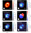 |
Fig. 1 Emission map of the 0.9 mm continuum Keplerian-masked integrated-intensity maps of the individual and stacked SO transitions, and the SO stacked intensity-weighted velocity and peak emission maps. The beam size is shown in the bottom left corner of each panel, and the images were constructed using a Briggs robust parameter of +0.5. |
3.4 Radial emission profile
Further information on the SO emitting region(s) can be gained from the spectra. Using the tool GoFish2 (Teague 2019), we shifted and stacked the spectra from each pixel in the channel maps. The spectra were extracted from annuli with a width of 0″.05. This analysis revealed a clear second ring of SO in the outer disk, and the resulting radial emission profile for the stacked image is shown in Fig. 3. The errors in this profile were calculated per radial bin from the rms in the shifted spectra. This outer ring is also tentatively present in the azimuthally averaged radial profiles from the intensity maps (shown in Fig. B.3), and the spectral stacking confirms this feature. In Fig. 3 we also compare these line radial profiles to the profile of our 0.9 mm continuum data imaged at the same weighting. The second SO ring peaks slightly beyond the peak of the second dust ring at ≈200 au. These profiles were extracted assuming a flat emitting surface. The spatial resolution is not high enough to constrain an emission surface for the SO emission; however, as discussed in Law et al. (2021), for more extreme emission heights of z/r ≈ 0.1–0.5, the shape and structure of the radial emission profiles are not significantly altered.
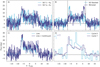 |
Fig. 2 Spectra extracted from a 0″.6 ellipse. (A) Individual transitions. (B) Spectra of the two stacked SO lines, and the same spectra mirrored. (C) Spectra of the two stacked SO lines with continuum subtraction and without continuum subtraction in the UV domain (after subtracting the average value of the line-free continuum emission channels). (D) Spectra of the two stacked SO lines from the ALMA Cycle 0 observations presented in Booth et al. (2018) and the Cycle 7 observations presented in this work. The Cycle 7 data have been imaged at 1.0 km s−1 in order to make a direct comparison to the Cycle 0 data. The noise calculated from the line-free channels in each respective spectrum is shown by a bar in the top left corner of the plot. |
3.5 Column density of SO
The radial emission profiles can be converted into a radial column density of SO under a few assumptions. Following a similar analysis as Loomis et al. (2018) and Terwisscha van Scheltinga et al. (2021), for example, we assumed that the lines are optically thin, in local-thermodynamic equilibrium, and because not enough transitions are detected over a range of upper energy levels in order to perform a meaningful rotational diagram analysis, we fixed the rotational temperature (Trot). For the inner disk (<100 au), Trot was chosen as 75, 100, and 200 K, and in the outer disk, (>100 au) 30, 40, and 50 K were chosen. These are reasonable given the values of the dust and gas temperatures in the HD 100546 physical model from Kama et al. (2016b). The resulting radial column density profile is the average of the two detected transitions and is shown in Fig. 3, where the errors are propagated from the errors in the stacked radial emission profile. For all values of Trot, the line is optically thin across the entirety of the disk. If the width of the emitting area of the SO in the inner ring were much narrower than we observe, then the optical depth and therefore column density we derive may be underestimated.
The azimuthal asymmetry is particularly interesting to investigate to determine how this variation affects the column density in the inner disk. Azimuthal profiles were extracted from the integrated-intensity maps at 20 au (the radius at which the SO peaks) and converted into column density. The azimuthal variation in integrated flux and column density of a factor of 2 is shown in Fig. 4. This might either be due to a chemical asymmetry, that is, there are more SO molecules on the southern side of the disk than on the northern side, or to a radiative transfer effect due to a temperature asymmetry. If the column density of SO is constant around the inner disk, then a temperature variation of ≈ ×2 is required between the north and south sides of the disk, assuming that the emission is indeed optically thin.
We also estimated the average SO column density in the inner disk and the upper limits on the SiO an SiS column densities. This was done using the integrated fluxes as listed in Table 1 and an assumed emitting area of the 0″.6 ellipse (1.8 × 10⁻¹¹ steradians) from which the spectra were extracted. We note that these average values underestimate the column density when compared to the radially and azimuthally resolved analysis. However, these are reasonable values to calculate in order to place upper limits on the SiO/SO and SiS/SO ratios and better place the SO detection in context with the range of non-detections in the literature. The results of these calculations are listed in Table 2, where the ratios of the column densities are SiO/SO < 1.4% and SiS/SO < 5%.
4 Discussion
4.1 Morphology of the SO emission
The SO emission detected in the HD 100546 disk is constrained to two rings. This double-ring structure closely follows that of the millimeter dust disk. From the kinematics, the SO emission is detected down to ≈ 10–15 au and therefore traces gas within the millimeter dust cavity (e.g. Pineda et al. 2019). There is a clear brightness asymmetry in the inner ring of SO of a factor of 2. The outer SO ring is located from 160 to 240 au, peaking just beyond the second dust ring, and is a factor of 100 times lower in peak flux than the inner ring. In comparison, the contrast ratio of the inner and outer dust rings is ≈1000. There is also a shoulder of SO emission outside of the inner dust ring out to ≈90 au. In the following sections, we discuss the chemical and/or physical processes that could lead to the distribution of SO that we observe in the HD 100546 disk.
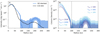 |
Fig. 3 Radial emission and column density profiles of the SO in the HD 100546 disk. (A) Azimuthally averaged intensity profiles for the stacked SO emission and 0.9 mm continuum emission. (B) Radial SO column density calculated at a range of rotational temperatures. |
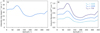 |
Fig. 4 Azimuthal emission and column density profiles of the SO in the HD 100546 disk. (A) Azimuthal intensity profile for the stacked SO emission at 20 au. (B) Azimuthal column density calculated at a range of rotational temperatures at 20 au. |
Average column densities for the inner 0″.6 of the HD 100546 disk for the detected and non-detected molecules.
4.2 Chemical origin of SO
SO has been proposed as a tracer of a variety of physical and chemical processes across star, disk, and planet formation, including (accretion) shocks, proto-stellar outflows, magneto-hydrodynamics driven disk winds and the sublimation of ices around hot cores (Sakai et al. 2014, 2017; Tabone et al. 2017; Lee et al. 2018; Taquet et al. 2020; van Gelder et al. 2021; Tychoniec et al. 2021). However, detections of SO in the more evolved Class II planet-forming disks are scarce. HD 100546 is one of only three disks in which SO has been imaged, the others being AB Aur and IRS 48 (Pacheco-Vázquez et al. 2016; Booth et al. 2021a). As well as the general problem in astrochemistry of sulphur depletion in dense gas (e.g. Tieftrunk et al. 1994; Laas & Caselli 2019), the lack of SO in many disks has been linked to an overall observed depletion of volatile oxygen relative to carbon (e.g. Miotello et al. 2017). The SO to CS ratio has therefore been explored as a tracer of the gas-phase C/O ratio in disks (Semenov et al. 2018; Le Gal et al. 2019, 2021; Fedele & Favre 2020). For example, Semenov et al. (2018) showed that the relative column densities of SO and CS decrease and increase by a factor of ≈100, respectively, when changing the elemental C/O ratio from 0.45 to 1.2. This means that at an elevated C/O ratio, CS traces the bulk of the gas-phase volatile sulphur in disks. This is consistent with observations of CS in disks where C2H, another tracer of an elevated C/O environment, is detected (e.g. Facchini et al. 2021). However, the inferred S/H ratios from modelling CS emission from disks are low, ≈8 × 10⁻⁸, indicating that a significant S reservoir is still locked in the ices or in a more refractory component (e.g. Le Gal et al. 2021). There are some caveats in the chemical models of sulphur in disks, namely, the initial partitioning of S in the ices, the completeness of the sulphur grain surface reaction networks, and photo-desorption yields that remain uncertain. All of these processes and assumptions are important if the observed gas-phase molecules have an ice origin. The level of oxygen (and carbon) depletion in HD 100546 has been modelled by Kama et al. (2016b), who found no evidence that oxygen is significantly more depleted than carbon throughout this warm disk unlike in other, cooler disks, such as TW Hya (Kama et al. 2016b). This leads to the expectation that some level of gas-phase SO is present through the entire disk.
From the high column density, and because the location of the SO emission is in the inner region of the HD 100546 disk, it is most likely that the SO originates from thermal desorption of S-rich ices. This is consistent with the evidence for warm 100-300 K dust and compact methanol emission from this same region of the disk (Mulders et al. 2011; Booth et al. 2021b). This release of S-ices at the edge of an inner dust cavity has been proposed by Kama et al. (2019), although the exact form of the S-ices (e.g. H2S, OCS, or SO2) is still unclear. SO can form efficiently in the gas phase via barrierless neutral-neutral reactions3, S + OH or O + SH if H2O and H2S ices are desorbed from the grains and subsequently photo-dissociated (see the discussion in Semenov et al. 2018),


OH has indeed been detected in the HD 100546 disk with the Photodetector Array Camera and Spectrometer (PACS) fon Herschel and originates from warm (200 K) gas (Fedele et al. 2013).
This ice sublimation scenario would predict an SO distribution that follows the large dust grain distribution and therefore should be broadly azimuthally symmetric; potential reasons for the observed asymmetry are discussed in Sects. 4.3 and 4.4. Overall, the SO (and CH3OH; Booth et al. 2021b) in the inner HD 100546 disk is similar to what has been observed in IRS 48 (van der Marel et al. 2021b; Booth et al. 2021a). In both of these warm Herbig transition disks, ice sublimation rather than gas-phase chemistry appears to cause most of the observable molecular column density. This is likely due to the close proximity of the dust (and ice) traps to the central stars. Future observations of other molecules will help to place these disks in better context of other well-characterised Herbig disks, such as HD 163296 and MWC 480 (Öberg et al. 2021).
Because the temperatures in the outer disk are much colder, the ring of SO that is co-spatial/beyond the dust ring at 200 au will have a different chemical origin. This is likely UV and/or cosmic-ray triggered desorption from icy dust grains. This would be similar to the explanation for the origin of H2CO emission in several disks, which shows an increase in column density at the edge of the millimeter dust disk (Loomis et al. 2015; Carney et al. 2017; Kastner et al. 2018; Pegues et al. 2020; Guzmán et al. 2021). Additionally, in a few sources, CS or SO is detected in a ring, approximately co-spatial with H2CO emission, beyond the millimetre-dust disk (Kastner et al. 2018; Le Gal et al. 2019; Podio et al. 2020; Rivière-Marichalar et al. 2020). Rings of H2CO and CH3OH aer also detected in this region of the HD 100546 disk, which would be consistent with this scenario (Booth et al. 2021b). Clear rings of SO and H2CO have also been observed in AB Aur just beyond the dust trap (Rivière-Marichalar et al. 2020). Although SO is detected in AB Aur, the models explored in Rivière-Marichalar et al. (2020) showed that the AB Aur data are most consistent with an elevated C/O = 1, a depleted sulphur abundance of 8 × 10⁻⁸, and an SO abundance of 4 × 10⁻¹⁰. The environment in the HD 100546 outer disk could be similar to this, but further models are needed to derive the gas-phase C/O and S/H across this disk.
In HD 100546, the depletion of SO in the dust gap and in the outer disk where CO is still abundant may be an indication of an elevated C/O ratio in the disk gas. This could be explained by volatile transport and an enhancement of S and O-rich ices in the millimetre-dust rings with peaks of SO emission just outside the rings and depletion in the regions without millimetre-dust. Additionally or alternatively, if SO is present in the gas-phase throughout the entire gas disk, there could be a depletion of the total gas column density in the outer millimetre-dust gap that might reduce the SO column below our detection limit; however, no clear CO gaps have been detected (e.g. Pineda et al. 2019). It is interesting to note that H2O ice and emission from cold H2O gas has been detected within the gap region from ≈40–150 au (Honda et al. 2016, van Dishoeck et al. 2021, Pirovano et al. 2022). Dedicated models of chemistry in planet-carved dust gaps show that it is important to also consider chemical processing in dust gaps, which will also affect the relative abundances of different gas tracers (Alarcón et al. 2021). Further disk-specific chemical models and observations of complementary molecules are needed to better constrain the chemical conditions in the HD 100546 disk.
4.3 Origin of the SO asymmetry
The bulk of the SO emission in the HD 100546 disk traces gas just within the millimeter dust cavity. The asymmetry in the detected emission ring could be due to an azimuthal variation in the SO abundance and/or disk temperature. This is distinct to the CS asymmetries presented in Le Gal et al. (2021) for the five disks in the sample from the ALMA large program “Molecules with ALMA at Planet-Forming Scales” (AS209, GM Aur, IM Lup, HD 163296, and MWC 480). In these other disks, the asymmetry is across the near and far sides of the disks, so that it might just be due to our viewing angles of the systems; however, in HD 100546, the asymmetry is not across this axis. In this section, we discuss potential origins of the SO asymmetry in the HD 100546 disk.
Booth et al. (2018) attributed the SO emission to a disk wind due to excess blueshifted emission in the line profile (see Fig. 2). In these Cycle 0 data, the emission was spatially unresolved and the kinematics appeared non-Keplerian. The stacked spectra from Booth et al. (2018) are shown in Fig. 2, where the emission peaks at the source velocity and the line profile has an excess blueshifted component. This interpretation of the data was very plausible since it has been shown that HD 100546 drives a jet (Schneider et al. 2020) and SO has also been shown to be a tracer of MHD driven disk winds (Tabone et al. 2020). The stacked spectra from the new Cycle 7 data presented in this work are compared to the Cycle 0 data in Fig. 2. In this figure, the Cycle 7 data are imaged at 1.0 km s−1 in order to make a direct comparisons to the Cycle 0 data. The two line profiles are noticeably different. The Cycle 0 data were taken in November 2012 and the Cycle 7 data in June 2021, that is, over a ≈ 8.5 yr baseline. Figure B.4 shows the residual spectra of the Cycle 7 spectra subtracted from the Cycle 0 spectra. The emission in the central channel, where V = V5SLSRK, remains above the ±3 σ level. Here, σ is the rms of each respective spectra added in quadrature. The overall line profile in the Cycle 7 data is symmetric in velocity about the source velocity compared to the Cycle 0 spectra. The Cycle 7 data therefore do not strongly support the disk wind hypothesis. Whilst we still see a brightness asymmetry, we do not see an additional component of emission that could be attributed to a disk wind.
A potential origin for the SO brightness asymmetry is an azimuthal temperature variation that might be caused by a warp. An extreme warp in the inner 100 au of the disk was suggested by Walsh et al. (2017) from ALMA observations of 12CO and previously, a warp was suggested by Panic et al. (2010) as an interpretation for asymmetric line observations from APEX. A similarly asymmetric line profile was traced in APEX CO J = 6 − 5 data also (Kama et al. 2016a). However, a warped disk has not been directly confirmed in higher-resolution ALMA line observations (e.g. Pineda et al. 2019; Pérez et al. 2020; Casassus et al. 2022). SO has been shown to be a potential chemical tracer of a warped disk by Young et al. (2021), where the variation SO abundance is primarily driven by the changes in X-ray illumination around the disk. In these generic models, the warp is caused by a 6.5 MJup planet embedded in a disk at 5 au on a 12° misaligned orbit (Nealon et al. 2019). On sub-au scales, the inner disk has been traced by Bohn et al. (2022) via Very Large Telescope Interferometer instrument GRAVITY (VLTI/GRAVITY) observations, but the position and inclination angles vary only by ≈4° compared to the outer disk traced in CO. It is unclear if a warp of this degree could create the temperature or chemical gradient we observe. In addition, current warp chemical models do not have large millimetre-dust cavities like that observed in the HD 100546 system (e.g. Young et al. 2021). This different disk structure would be expected to alter the signature of the warp in the line emission.
Sulphur monoxide is also a known tracer of shocks. In particular, it has been proposed as a tracer of accretion shocks at the disk envelope interface in younger class 0/I sources (Sakai et al. 2014, Sakai et al. 2017; Aota et al. 2015; Artur de la Villarmois et al. 2019; van Gelder et al. 2021; Garufi et al. 2021). SO is therefore a potential tracer of accretion shocks into a CPD. So far, there are only upper limits on the CPD dust mass in the HD 100546 cavity (Pineda et al. 2019). In our data, we also have a non-detection of another shock tracer SiO with an average SiO/SO ratio of <1.4%. This is an indication that if SO is enhanced in the inner disk due to a shock, then the strength of the shock is not sufficient for the sputtering of the grain cores and is limited to the removal of ices. In this case, a weak shock is almost chemically indistinct from thermal ice sublimation at warm temperatures (≳ 100 K) because in both scenarios, the full ice mantle is removed from the dust grains without chemical alteration. Other tracers of gas within the cavity have shown asymmetries. The CO ro-vibrational lines observed with the CRyogenic high-resolution InfraRed Echelle Spectrograph on the VLT (VLT/CRIRES) have been shown to trace the warm gas from the inner rim of the outer disk (Hein Bertelsen et al. 2014). The Doppler shift of the CO v = 1–0 P(26) line has been shown to be time variable, tracing a hotspot of CO gas that is now behind the near side of the cavity wall (Brittain et al. 2009, 2013, 2014, 2019). The interpretation of this emission is hot gas associated with a CPD of a super-Jovian planet. An asymmetry in the OH emission that matches the blueshifted asymmetry in the SO emission is also observed with VLT/CRIRES, but this asymmetry in the VLT/CRIRES data can be explained as an instrumental effect when the slit width, which was smaller than the diameter of the cavity, is misaligned (Fedele et al. 2015). This is not an issue for the CO observations, which were taken with a slit size larger than the cavity diameter (Brittain et al. 2019).
4.4 Connections to ongoing giant planet formation in the disk
There are multiple complementary observations of the HD 100546 disk that suggest the presence of a giant planet within the millimeter dust cavity with an inferred orbital radius of HD 100546c c of ≈ 10–15 au. Here we discuss how the asymmetry in the SO emission may be related to this putative forming planet. Figure 5 shows the high-resolution 0.9 mm continuum data from Pineda et al. (2019) with a contour overlay of the stacked SO integrated-intensity and peak intensity maps imaged with a Briggs robust parameter of 0.0. Also highlighted are the locations of three features in the disk that are potentially linked to forming giant planets. The first is a point source identified via observations with the Gemini Planet Imager that has been attributed to either the inner edge of the dust cavity wall or forming planet HD 100546 c (Currie et al. 2015). Additionally, the CO ro-vibrational observations are compatible with an orbiting companion within the cavity where the excess CO emission is proposed to be tracing gas in a CPD (Brittain et al. 2009, 2013, 2014, 2019). The ≈15 -yr baseline of CO observations has allowed for an inferred orbital radius of 10.5–12.3 au. This is approximately the same distance from the star as the region identified as HD 100546 c. The third feature is a potential planet detected via the Doppler flip in the 12CO kinematics as observed by ALMA. Casassus & Pérez (2019) and Casassus et al. (2022) attributed this Doppler flip to a forming planet or planetary wake originating from an annular groove inside the main continuum ring at ≈25 au.
The peak of the SO emission is co-spatial with the location of HD 100546 c according to the scattered-light observations of Currie et al. (2015) and the excess CO signal in 2017 from Brittain et al. (2019). Forming planets in disks have been shown in models to heat the local disk environment through their inherent accretion luminosity, and this will affect the observable disk chemistry (Cleeves et al. 2015). In the chemical models from Cleeves et al. (2015), SO is not specifically explored as a tracer of this ice sublimation, but H2S and CS do show enhancements in abundance and line strength in the same azimuthal region as the planet. The optimal tracers of this process will strongly depend on where the planet is located in the disk and on the temperature, for instance, if it is warm enough to liberate H2O ice. However, overall, an enhancement in SO in the disk due to HD 100546 c is a plausible explanation for our observations. The SO observations from Cycles 0 and 7 are taken 8.5 yr apart, which is about one-fifth of an orbit for a planet at 10 au. Therefore, some variation in the SO emission detected at these two epochs as a result of a planet in the cavity is feasible. The spectra presented in panel D of Fig. 2 are different. The movement of the peak in the spectra from ≈0 km s−1 to ≈ − 7 km s−1 is consistent with the anti-clockwise rotation of a hotspot in the disk from approximately the minor axis to the south of the disk. Booth et al. (2018) showed that the SO emission was asymmetric, peaking on the east side of the disk minor axis, and this was also traced by a brightness asymmetry in the optically thick 12CO J = 3−2 emission (Walsh et al. 2017). With the SO peaking now in the south of the disk in the Cycle 7 observations, this is generally consistent with rotation of a hotspot of molecular gas in the cavity or at the cavity edge; however, this signature seems to be trailing that of the CO ro-vibrational lines. SO could therefore be tracing the chemistry in the post shock regime, that is, behind the orbit of the planet. The CPD models of Szulágyi (2017) for 10 MJup planets, like that expected for HD 100546 c, show very high temperatures within 0.1 times the Hill sphere (>1000 K), allowing dust to sublimate and likely destroying most molecules. However, in the outer regions of the CPD, the temperature can drop to a few 100 K, and with densities of ≈1014 cm−3, this could be a favourable environment for a rich, high-temperature gas-phase chemistry. The SO may not directly trace accretion shocks from the HD 100546 c CPD, especially as SiO is not detected in these data, but rather the impact of HD 100546 c on the surrounding disk, and in particular, the exposed cavity wall. In this contect, it is interesting to note that a giant planet in a disk can excite the orbits of planetesimals embedded in the gas disk, resulting in bow-shock heating that can evaporate ices (Nagasawa et al. 2019).
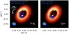 |
Fig. 5 Composite image showing the 0.9 mm dust emission from Pineda et al. (2019), the [30,35,40]×σ (where σ is the rms noise of an integrated-intensity map generated without a Keplerian mask over the same number of channels) contours of the stacked SO Keplerian-masked integrated-intensity map (left) and the [5,6,7,8]×σ (where σ is the channel map noise) contours of the peak intensity map (right) imaged with a Briggs robust parameter of 0.0. The location of the putative planet HD 100546 c (purple, Currie et al. 2015) and the putative planet from (Casassus & Pérez 2019, green) are highlighted with circles. The excess CO signal from Brittain et al. 2019 in 2017 is shown by the white star symbol. Beams for the continuum observations (orange) and the line data (blue) are shown in the bottom left corner. The arrow marks the orbital direction of the disk material and planet(s). |
5 Conclusions
This paper presented ALMA observations of sulphur monoxide emission from the HD 100546 disk at ≈20 au resolution, showing that the dust and this gas tracer are closely linked. The SO is detected in two main rings that follow the ringed distribution of the millimetre-dust disk. These two rings of molecular emission are linked to ices in the disk, but have different chemical origins: thermal and non-thermal ice sublimation. The innerring gas is detected down to ≈10–15 au, which is within the millimetre-dust cavity. The mechanism of thermal sublimation of S-rich ices (e.g. H2S) in this region of the disk is consistent with the detection of gas-phase CH3OH which requires an ice origin (Booth et al. 2021b). In the outer disk, SO is co-spatial with rings of H2CO and CH3OH which all likely originate from non-thermal desorption (Booth et al. 2021b). However, disk-specific gas-grain chemical models are needed to confirm this, and additional models are required to determine the C/O and S/H ratio of the gas across the disk. The asymmetry in the SO emission from the inner disk might trace the impact of the forming giant planet HD 100546 c on the local disk chemistry directly or indirectly. Observations of other gas tracers at sub-mm wavelengths, such as higher J CO lines, and observations of the cavity gas with complementary telescopes, for instance VLT/CRIRES+, will help to determine whether SO is indeed a molecular tracer of giant planet formation. Furthermore, chemical and radiative transfer models to investigate the survival and observability of molecules in CPDs and the disk region within the sphere of influence of a forming giant planet are also needed to test the hypothesis we suggested for a planet origin of the SO asymmetry in the HD 100546 disk.
Acknowledgements
Authors thank Prof. Michiel Hogerheijde, Dr. Miguel Vioque, Dr. Alison Young and Dr. Sarah K. Leslie for useful discussions. Astrochemistry in Leiden is supported by the Netherlands Research School for Astronomy (NOVA), by funding from the European Research Council (ERC) under the European Union’s Horizon 2020 research and innovation programme (grant agreement No. 101019751 MOLDISK). ALMA is a partnership of ESO (representing its member states), NSF (USA) and NINS (Japan), together with NRC (Canada) and NSC and ASIAA (Taiwan) and KASI (Republic of Korea), in cooperation with the Republic of Chile. The Joint ALMA Observatory is operated by ESO, AUI/ NRAO and NAOJ. CW acknowledges support from the University of Leeds, STFC, and UKRI (grant numbers ST/T000287/1, MR/T040726/1) This paper makes use of the following ALMA data: 2011.0.00863.S, 2015.1.00806.S, 2019.1.00193.S.
Appendix A Observing setup
Observing setup for ALMA Band 7 program 2019.1.00193.S (PI: A. S. Booth)
Appendix B tCLEAN robust grid images and image parameters
Image properties of the 0.9 mm continuum integrated-intensity maps and stacked SO channel maps for a range of Briggs robust parameters 0.9 mm Continuum
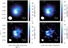 |
Fig. B.1 Keplerian-masked integrated-intensity maps of the stacked SO emission generated over a range of Briggs robust parameters (+1.0, +0.5, 0.0, and −0.5). The resulting beams are shown in the bottom left corner of each panel, and the sizes are listed in Table A.1. |
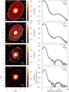 |
Fig. B.2 Left: HD 100546 0.9 mm continuum maps with a range of Briggs robust parameters (+1.0, +0.5, 0.0, and −0.5). The white contours mark the σ ×[3,5] level for each map, where σ is the rms, as listed in Table B.1. Right: Azimuthally averaged and deprojected radial emission profiles for each of the maps. The error bars are calculated from the standard deviation of the pixel values in each bin divided by the square root of the number of beams per annulus. In the top right corner of each panel, the major axis of the beam is represented by a black line. |
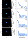 |
Fig. B.3 Left: HD 100546 stacked SO Keplerian-masked integrated-intensity maps with a range of Briggs robust parameters (+1.0, +0.5, 0.0, and −0.5). Right: Azimuthally averaged and deprojected radial emission profiles for each of the maps, with the matching continuum radial profile normalised to the peak in the line radial profile. The error bars are calculated from the standard deviation of the pixel values in each bin divided by the square root of the number of beams per annulus. In the top right corner of each panel, the major axis of the beam is represented by a black line. |
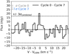 |
Fig. B.4 Residual spectra of the Cycle 7 spectra subtracted from the Cycle 0 spectra of the stacked SO emission, as shown in Figure 2. The noise calculated from the line-free channels in each respective spectrum is shown by a bar in the top left corner of the plot. The dashed line shows the ±3 σ level, where σcombined is the rms of each respective spectrum added in quadrature. |
Appendix C Detection of new sub-millimeter source near HD 100546
We report the detection of a new sub-millimeter source located at a projected separation from HD 100546 of 9/34 with a position angle of 37.7° east of north. The peak in continuum emission is at RA:173.360° Dec:-70.193° and reaches a signal-to-noise ratio of 5 in the continuum image with Briggs robust weighting of +1.0 and has a flux density of 1 mJy. A number of previously identified background stars to HD 100546 lie within our field of view (Grady et al. 2001; Ardila et al. 2007). The nearest source is field star 9 from Table 3 in Ardila et al. (2007), who concluded from the photometry that this is a background star relative to HD 100546 and that due to the reddening, it is within or behind the dark cloud DC296.2-7.9 (Vieira et al. 1999). Follow-up observations of HD 100546 and the surrounding environment with Gemini/NICI confirmed their background nature as no significant proper motion of these sources is detected, whereas HD 100546 has moved (Boccaletti et al. 2013). From GAIA DR3, we investigated the locations of all known sources within our field of view in Figure B1 and plot them alongside our continuum map and the sources from Grady et al. (2001). None of the known sources match the location of our new sub-mm source. The emission we detect may be associated with an envelope or disk around a background star that may be young and not optically visible due to both its own envelope or disk and the cloud. As there is no distance measurement to this object, any inferred dust mass is highly uncertain. Alternatively, the source we detect might be a background galaxy. We estimated the likelihood of this using the ALMA 1.1 mm survey from Hatsukade et al. (2016). From this, we would naively expect ≈0.1 extragalactic sources of S>1 mJy in our primary beam, and so the possibility of this source being a background galaxy may be unlikely, but cannot be discounted.
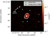 |
Fig. C.1 HD 100546 0.9 mm continuum maps with a Briggs robust parameter of +1.0. The white contours mark the σ ×[4,5,6] level for each map, where σ is the rms, as listed in Table A.1. The background stars identified by GAIA DR3 are shown with green crosses, and the blue crosses are from Grady et al. (2001). |
References
- Alarcón, F., Bosman, A. D., Bergin, E. A., et al. 2021, ApJS, 257, 8 [CrossRef] [Google Scholar]
- ALMA Partnership, Brogan, C. L., Pérez, L. M., et al. 2015, ApJ, 808, L3 [Google Scholar]
- Andrews, S. M., Huang, J., Pérez, L. M., et al. 2018, ApJ, 869, L41 [NASA ADS] [CrossRef] [Google Scholar]
- Aota, T., Inoue, T., & Aikawa, Y. 2015, ApJ, 799, 141 [NASA ADS] [CrossRef] [Google Scholar]
- Ardila, D. R., Golimowski, D. A., Krist, J. E., et al. 2007, ApJ, 665, 512 [Google Scholar]
- Artur de la Villarmois, E., Jørgensen, J. K., Kristensen, L. E., et al. 2019, A&A, 626, A71 [NASA ADS] [CrossRef] [EDP Sciences] [Google Scholar]
- Banzatti, A., Pascucci, I., Bosman, A. D., et al. 2020, ApJ, 903, 124 [NASA ADS] [CrossRef] [Google Scholar]
- Benisty, M., Bae, J., Facchini, S., et al. 2021, ApJ, 916, L2 [NASA ADS] [CrossRef] [Google Scholar]
- Bergin, E. A., Du, F., Cleeves, L. I., et al. 2016, ApJ, 831, 101 [Google Scholar]
- Boccaletti, A., Pantin, E., Lagrange, A. M., et al. 2013, A&A, 560, A20 [NASA ADS] [CrossRef] [EDP Sciences] [Google Scholar]
- Bohn, A. J., Benisty, M., Perraut, K., et al. 2022, A&A, 658, A183 [NASA ADS] [CrossRef] [EDP Sciences] [Google Scholar]
- Booth, R. A., & Ilee, J. D. 2019, MNRAS, 487, 3998 [CrossRef] [Google Scholar]
- Booth, R. A., Clarke, C. J., Madhusudhan, N., & Ilee, J. D. 2017, MNRAS, 469, 3994 [Google Scholar]
- Booth, A. S., Walsh, C., Kama, M., et al. 2018, A&A, 611, A16 [NASA ADS] [CrossRef] [EDP Sciences] [Google Scholar]
- Booth, A. S., van der Marel, N., Leemker, M., van Dishoeck, E. F., & Ohashi, S. 2021a, A&A, 651, L6 [NASA ADS] [CrossRef] [EDP Sciences] [Google Scholar]
- Booth, A. S., Walsh, C., Terwisscha van Scheltinga, J., et al. 2021b, Nat. Astron., 5, 684 [NASA ADS] [CrossRef] [Google Scholar]
- Brittain, S. D., Najita, J. R., & Carr, J. S. 2009, ApJ, 702, 85 [Google Scholar]
- Brittain, S. D., Najita, J. R., Carr, J. S., et al. 2013, ApJ, 767, 159 [NASA ADS] [CrossRef] [Google Scholar]
- Brittain, S. D., Carr, J. S., Najita, J. R., Quanz, S. P., & Meyer, M. R. 2014, ApJ, 791, 136 [Google Scholar]
- Brittain, S. D., Najita, J. R., & Carr, J. S. 2019, ApJ, 883, 37 [NASA ADS] [CrossRef] [Google Scholar]
- Brunken, N. G. C., Booth, A. S., Leemker, M., et al. 2022, A&A, 659, A29 [NASA ADS] [CrossRef] [EDP Sciences] [Google Scholar]
- Carney, M. T., Hogerheijde, M. R., Loomis, R. A., et al. 2017, A&A, 605, A21 [NASA ADS] [CrossRef] [EDP Sciences] [Google Scholar]
- Carney, M. T., Hogerheijde, M. R., Guzmán, V. V., et al. 2019, A&A, 623, A124 [NASA ADS] [CrossRef] [EDP Sciences] [Google Scholar]
- Casassus, S., & Pérez, S. 2019, ApJ, 883, L41 [Google Scholar]
- Casassus, S., Cárcamo, M., Hales, A., Weber, P., & Dent, B. 2022, ApJ, 933, L4 [NASA ADS] [CrossRef] [Google Scholar]
- Cazzoletti, P., van Dishoeck, E. F., Visser, R., Facchini, S., & Bruderer, S. 2018, A&A, 609, A93 [NASA ADS] [CrossRef] [EDP Sciences] [Google Scholar]
- Cleeves, L. I., Bergin, E. A., & Harries, T. J. 2015, ApJ, 807, 2 [NASA ADS] [CrossRef] [Google Scholar]
- Currie, T., Cloutier, R., Brittain, S., et al. 2015, ApJ, 814, L27 [Google Scholar]
- Currie, T., Brittain, S., Grady, C. A., Kenyon, S. J., & Muto, T. 2017, Res. Notes Am. Astron. Soc., 1, 40 [Google Scholar]
- Currie, T., Biller, B., Lagrange, A.-M., et al. 2022, ArXiv e-prints [arXiv:2205.05696] [Google Scholar]
- Czekala, I., Loomis, R. A., Teague, R., et al. 2021, ApJS, 257, 2 [NASA ADS] [CrossRef] [Google Scholar]
- Facchini, S., Teague, R., Bae, J., et al. 2021, AJ, 162, 99 [NASA ADS] [CrossRef] [Google Scholar]
- Favre, C., Fedele, D., Maud, L., et al. 2019, ApJ, 871, 107 [Google Scholar]
- Fedele, D., & Favre, C. 2020, A&A, 638, A110 [NASA ADS] [CrossRef] [EDP Sciences] [Google Scholar]
- Fedele, D., Bruderer, S., van Dishoeck, E. F., et al. 2013, A&A, 559, A77 [CrossRef] [EDP Sciences] [Google Scholar]
- Fedele, D., Bruderer, S., van den Ancker, M. E., & Pascucci, I. 2015, ApJ, 800, 23 [Google Scholar]
- Fedele, D., Toci, C., Maud, L., & Lodato, G. 2021, A&A, 651, A90 [NASA ADS] [CrossRef] [EDP Sciences] [Google Scholar]
- Follette, K. B., Rameau, J., Dong, R., et al. 2017, AJ, 153, 264 [Google Scholar]
- Garufi, A., Podio, L., Codella, C., et al. 2022, A&A, 658, A104 [CrossRef] [EDP Sciences] [Google Scholar]
- Grady, C. A., Polomski, E. F., Henning, T., et al. 2001, AJ, 122, 3396 [Google Scholar]
- Guzmán, V. V., Bergner, J. B., Law, C. J., et al. 2021, ApJS, 257, 6 [CrossRef] [Google Scholar]
- Hatsukade, B., Kohno, K., Umehata, H., et al. 2016, Pasj, 68, 36 [NASA ADS] [CrossRef] [Google Scholar]
- Hein Bertelsen, R. P., Kamp, I., Goto, M., et al. 2014, A&A, 561, A102 [NASA ADS] [CrossRef] [EDP Sciences] [Google Scholar]
- Honda, M., Kudo, T., Takatsuki, S., et al. 2016, ApJ, 821, 2 [NASA ADS] [CrossRef] [Google Scholar]
- Jiang, H., Zhu, W., & Ormel, C. W. 2022, ApJ, 924, L31 [NASA ADS] [CrossRef] [Google Scholar]
- Jorsater, S., & van Moorsel, G. A. 1995, AJ, 110, 2037 [Google Scholar]
- Kama, M., Bruderer, S., Carney, M., et al. 2016a, A&A, 588, A108 [NASA ADS] [CrossRef] [EDP Sciences] [Google Scholar]
- Kama, M., Bruderer, S., van Dishoeck, E. F., et al. 2016b, A&A, 592, A83 [NASA ADS] [CrossRef] [EDP Sciences] [Google Scholar]
- Kama, M., Shorttle, O., Jermyn, A. S., et al. 2019, ApJ, 885, 114 [Google Scholar]
- Kastner, J. H., Qi, C., Dickson-Vandervelde, D. A., et al. 2018, ApJ, 863, 106 [Google Scholar]
- Krijt, S., Schwarz, K. R., Bergin, E. A., & Ciesla, F. J. 2018, ApJ, 864, 78 [Google Scholar]
- Krijt, S., Bosman, A. D., Zhang, K., et al. 2020, ApJ, 899, 134 [NASA ADS] [CrossRef] [Google Scholar]
- Laas, J. C., & Caselli, P. 2019, A&A, 624, A108 [NASA ADS] [CrossRef] [EDP Sciences] [Google Scholar]
- Law, C. J., Loomis, R. A., Teague, R., et al. 2021, ApJS, 257, 3 [NASA ADS] [CrossRef] [Google Scholar]
- Lee, C.-F., Li, Z.-Y., Hirano, N., et al. 2018, ApJ, 863, 94 [NASA ADS] [CrossRef] [Google Scholar]
- Le Gal, R., Öberg, K. I., Loomis, R. A., Pegues, J., & Bergner, J. B. 2019, ApJ, 876, 72 [Google Scholar]
- Le Gal, R., Öberg, K. I., Teague, R., et al. 2021, ApJS, 257, 12 [NASA ADS] [CrossRef] [Google Scholar]
- Leemker, M., van’t Hoff, M. L. R., Trapman, L., et al. 2021, A&A, 646, A3 [EDP Sciences] [Google Scholar]
- Loomis, R. A., Cleeves, L. I., Öberg, K. I., Guzman, V. V., & Andrews, S. M. 2015, ApJ, 809, L25 [Google Scholar]
- Loomis, R. A., Cleeves, L. I., Öberg, K. I., et al. 2018, ApJ, 859, 131 [Google Scholar]
- McMullin, J. P., Waters, B., Schiebel, D., Young, W., & Golap, K. 2007, ASP Conf. Ser., 376, 127 [Google Scholar]
- Miley, J. M., Panic, O., Haworth, T. J., et al. 2019, MNRAS, 485, 739 [NASA ADS] [CrossRef] [Google Scholar]
- Miotello, A., van Dishoeck, E. F., Williams, J. P., et al. 2017, A&A, 599, A113 [NASA ADS] [CrossRef] [EDP Sciences] [Google Scholar]
- Mulders, G. D., Waters, L. B. F. M., Dominik, C., et al. 2011, A&A, 531, A93 [NASA ADS] [CrossRef] [EDP Sciences] [Google Scholar]
- Nagasawa, M., Tanaka, K. K., Tanaka, H., et al. 2019, ApJ, 871, 110 [NASA ADS] [CrossRef] [Google Scholar]
- Nealon, R., Pinte, C., Alexander, R., Mentiplay, D., & Dipierro, G. 2019, MNRAS, 484, 4951 [CrossRef] [Google Scholar]
- Öberg, K. I., Guzmán, V. V., Walsh, C., et al. 2021, ApJS, 257, 1 [CrossRef] [Google Scholar]
- Pacheco-Vázquez, S., Fuente, A., Baruteau, C., et al. 2016, A&A, 589, A60 [Google Scholar]
- Panic, O., van Dishoeck, E. F., Hogerheijde, M. R., et al. 2010, A&A, 519, A110 [NASA ADS] [CrossRef] [EDP Sciences] [Google Scholar]
- Pegues, J., Öberg, K. I., Bergner, J. B., et al. 2020, ApJ, 890, 142 [Google Scholar]
- Pérez, S., Casassus, S., Hales, A., et al. 2020, ApJ, 889, L24 [Google Scholar]
- Pineda, J. E., Szulágyi, J., Quanz, S. P., et al. 2019, ApJ, 871, 48 [Google Scholar]
- Pinilla, P., Birnstiel, T., & Walsh, C. 2015, A&A, 580, A105 [NASA ADS] [CrossRef] [EDP Sciences] [Google Scholar]
- Pinte, C., van der Plas, G., Ménard, F., et al. 2019, Nat. Astron., 3, 1109 [NASA ADS] [CrossRef] [Google Scholar]
- Pirovano, L. M., Fedele, D., van Dishoeck, E. F., et al. 2022, A&A, 665, A45 [NASA ADS] [CrossRef] [EDP Sciences] [Google Scholar]
- Podio, L., Codella, C., Lefloch, B., et al. 2017, MNRAS, 470, L16 [Google Scholar]
- Podio, L., Garufi, A., Codella, C., et al. 2020, A&A, 644, A119 [NASA ADS] [CrossRef] [EDP Sciences] [Google Scholar]
- Pyerin, M. A., Delage, T. N., Kurtovic, N. T., et al. 2021, A&A, 656, A150 [NASA ADS] [CrossRef] [EDP Sciences] [Google Scholar]
- Quanz, S. P., Amara, A., Meyer, M. R., et al. 2013, ApJ, 766, L1 [Google Scholar]
- Quanz, S. P., Amara, A., Meyer, M. R., et al. 2015, ApJ, 807, 64 [Google Scholar]
- Rab, C., Kamp, I., Ginski, C., et al. 2019, A&A, 624, A16 [EDP Sciences] [Google Scholar]
- Rivière-Marichalar, P., Fuente, A., Le Gal, R., et al. 2020, A&A, 642, A32 [EDP Sciences] [Google Scholar]
- Sakai, N., Sakai, T., Hirota, T., et al. 2014, Nature, 507, 78 [Google Scholar]
- Sakai, N., Oya, Y., Higuchi, A. E., et al. 2017, MNRAS, 467, L76 [NASA ADS] [Google Scholar]
- Salinas, V. N., Hogerheijde, M. R., Mathews, G. S., et al. 2017, A&A, 606, A125 [NASA ADS] [CrossRef] [EDP Sciences] [Google Scholar]
- Schneider, P. C., Dougados, C., Whelan, E. T., et al. 2020, A&A, 638, L3 [NASA ADS] [CrossRef] [EDP Sciences] [Google Scholar]
- Schöier, F. L., van der Tak, F. F. S., van Dishoeck, E. F., & Black, J. H. 2005, A&A, 432, 369 [Google Scholar]
- Semenov, D., Favre, C., Fedele, D., et al. 2018, A&A, 617, A28 [NASA ADS] [CrossRef] [EDP Sciences] [Google Scholar]
- Sissa, E., Gratton, R., Garufi, A., et al. 2018, A&A, 619, A160 [NASA ADS] [CrossRef] [EDP Sciences] [Google Scholar]
- Szulágyi, J. 2017, ApJ, 842, 103 [Google Scholar]
- Tabone, B., Cabrit, S., Bianchi, E., et al. 2017, A&A, 607, L6 [NASA ADS] [CrossRef] [EDP Sciences] [Google Scholar]
- Tabone, B., Cabrit, S., Pineau des Forêts, G., et al. 2020, A&A, 640, A82 [CrossRef] [EDP Sciences] [Google Scholar]
- Taquet, V., Codella, C., De Simone, M., et al. 2020, A&A, 637, A63 [NASA ADS] [CrossRef] [EDP Sciences] [Google Scholar]
- Teague, R. 2019, J. Open Source Softw., 4, 1632 [NASA ADS] [CrossRef] [Google Scholar]
- Terwisscha van Scheltinga, J., Hogerheijde, M. R., Cleeves, L. I., et al. 2021, ApJ, 906, 111 [Google Scholar]
- Tieftrunk, A., Pineau des Forets, G., Schilke, P., & Walmsley, C. M. 1994, A&A, 289, 579 [Google Scholar]
- Toci, C., Lodato, G., Christiaens, V., et al. 2020a, MNRAS, 499, 2015 [NASA ADS] [CrossRef] [Google Scholar]
- Toci, C., Lodato, G., Fedele, D., Testi, L., & Pinte, C. 2020b, ApJ, 888, L4 [Google Scholar]
- Tychoniec, Ł., van Dishoeck, E. F., van’t Hoff, M. L. R., et al. 2021, A&A, 655, A65 [NASA ADS] [CrossRef] [EDP Sciences] [Google Scholar]
- van der Marel, N., van Dishoeck, E. F., Bruderer, S., et al. 2013, Science, 340, 1199 [Google Scholar]
- van der Marel, N., van Dishoeck, E. F., Bruderer, S., Pérez, L., & Isella, A. 2015, A&A, 579, A106 [NASA ADS] [CrossRef] [EDP Sciences] [Google Scholar]
- van der Marel, N., van Dishoeck, E. F., Bruderer, S., et al. 2016, A&A, 585, A58 [NASA ADS] [CrossRef] [EDP Sciences] [Google Scholar]
- van der Marel, N., Birnstiel, T., Garufi, A., et al. 2021a, AJ, 161, 33 [Google Scholar]
- van der Marel, N., Booth, A. S., Leemker, M., van Dishoeck, E. F., & Ohashi, S. 2021b, A&A, 651, L5 [NASA ADS] [CrossRef] [EDP Sciences] [Google Scholar]
- van Dishoeck, E. F., Kristensen, L. E., Mottram, J. C., et al. 2021, A&A, 648, A24 [NASA ADS] [CrossRef] [EDP Sciences] [Google Scholar]
- van Gelder, M. L., Tabone, B., van Dishoeck, E. F., & Godard, B. 2021, A&A, 653, A159 [CrossRef] [EDP Sciences] [Google Scholar]
- van Hoff, M. L. R., Walsh, C., Kama, M., Facchini, S., & van Dishoeck, E. F. 2017, A&A, 599, A101 [CrossRef] [EDP Sciences] [Google Scholar]
- Vieira, S. L. A., Pogodin, M. A., & Franco, G. A. P. 1999, A&A, 345, 559 [NASA ADS] [Google Scholar]
- Vioque, M., Oudmaijer, R. D., Baines, D., Mendigutía, I., & Pérez-Martínez, R. 2018, A&A, 620, A128 [NASA ADS] [CrossRef] [EDP Sciences] [Google Scholar]
- Walsh, C., Juhász, A., Pinilla, P., et al. 2014, ApJ, 791, L6 [Google Scholar]
- Walsh, C., Daley, C., Facchini, S., & Juhász, A. 2017, A&A, 607, A114 [NASA ADS] [CrossRef] [EDP Sciences] [Google Scholar]
- Young, A. K., Alexander, R., Walsh, C., et al. 2021, MNRAS, 505, 4821 [NASA ADS] [CrossRef] [Google Scholar]
- Zhang, K., Bergin, E. A., Schwarz, K., Krijt, S., & Ciesla, F. 2019, ApJ, 883, 98 [Google Scholar]
- Zhang, K., Bosman, A. D., & Bergin, E. A. 2020, ApJ, 891, L16 [NASA ADS] [CrossRef] [Google Scholar]
- Zhang, K., Booth, A. S., Law, C. J., et al. 2021, ApJS, 257, 5 [NASA ADS] [CrossRef] [Google Scholar]
- Zhang, S., Zhu, Z., Huang, J., et al. 2018, ApJ, 869, L47 [Google Scholar]
All Tables
Average column densities for the inner 0″.6 of the HD 100546 disk for the detected and non-detected molecules.
Image properties of the 0.9 mm continuum integrated-intensity maps and stacked SO channel maps for a range of Briggs robust parameters 0.9 mm Continuum
All Figures
|
Fig. 1 Emission map of the 0.9 mm continuum Keplerian-masked integrated-intensity maps of the individual and stacked SO transitions, and the SO stacked intensity-weighted velocity and peak emission maps. The beam size is shown in the bottom left corner of each panel, and the images were constructed using a Briggs robust parameter of +0.5. |
| In the text | |
|
Fig. 2 Spectra extracted from a 0″.6 ellipse. (A) Individual transitions. (B) Spectra of the two stacked SO lines, and the same spectra mirrored. (C) Spectra of the two stacked SO lines with continuum subtraction and without continuum subtraction in the UV domain (after subtracting the average value of the line-free continuum emission channels). (D) Spectra of the two stacked SO lines from the ALMA Cycle 0 observations presented in Booth et al. (2018) and the Cycle 7 observations presented in this work. The Cycle 7 data have been imaged at 1.0 km s−1 in order to make a direct comparison to the Cycle 0 data. The noise calculated from the line-free channels in each respective spectrum is shown by a bar in the top left corner of the plot. |
| In the text | |
|
Fig. 3 Radial emission and column density profiles of the SO in the HD 100546 disk. (A) Azimuthally averaged intensity profiles for the stacked SO emission and 0.9 mm continuum emission. (B) Radial SO column density calculated at a range of rotational temperatures. |
| In the text | |
|
Fig. 4 Azimuthal emission and column density profiles of the SO in the HD 100546 disk. (A) Azimuthal intensity profile for the stacked SO emission at 20 au. (B) Azimuthal column density calculated at a range of rotational temperatures at 20 au. |
| In the text | |
|
Fig. 5 Composite image showing the 0.9 mm dust emission from Pineda et al. (2019), the [30,35,40]×σ (where σ is the rms noise of an integrated-intensity map generated without a Keplerian mask over the same number of channels) contours of the stacked SO Keplerian-masked integrated-intensity map (left) and the [5,6,7,8]×σ (where σ is the channel map noise) contours of the peak intensity map (right) imaged with a Briggs robust parameter of 0.0. The location of the putative planet HD 100546 c (purple, Currie et al. 2015) and the putative planet from (Casassus & Pérez 2019, green) are highlighted with circles. The excess CO signal from Brittain et al. 2019 in 2017 is shown by the white star symbol. Beams for the continuum observations (orange) and the line data (blue) are shown in the bottom left corner. The arrow marks the orbital direction of the disk material and planet(s). |
| In the text | |
|
Fig. B.1 Keplerian-masked integrated-intensity maps of the stacked SO emission generated over a range of Briggs robust parameters (+1.0, +0.5, 0.0, and −0.5). The resulting beams are shown in the bottom left corner of each panel, and the sizes are listed in Table A.1. |
| In the text | |
|
Fig. B.2 Left: HD 100546 0.9 mm continuum maps with a range of Briggs robust parameters (+1.0, +0.5, 0.0, and −0.5). The white contours mark the σ ×[3,5] level for each map, where σ is the rms, as listed in Table B.1. Right: Azimuthally averaged and deprojected radial emission profiles for each of the maps. The error bars are calculated from the standard deviation of the pixel values in each bin divided by the square root of the number of beams per annulus. In the top right corner of each panel, the major axis of the beam is represented by a black line. |
| In the text | |
|
Fig. B.3 Left: HD 100546 stacked SO Keplerian-masked integrated-intensity maps with a range of Briggs robust parameters (+1.0, +0.5, 0.0, and −0.5). Right: Azimuthally averaged and deprojected radial emission profiles for each of the maps, with the matching continuum radial profile normalised to the peak in the line radial profile. The error bars are calculated from the standard deviation of the pixel values in each bin divided by the square root of the number of beams per annulus. In the top right corner of each panel, the major axis of the beam is represented by a black line. |
| In the text | |
|
Fig. B.4 Residual spectra of the Cycle 7 spectra subtracted from the Cycle 0 spectra of the stacked SO emission, as shown in Figure 2. The noise calculated from the line-free channels in each respective spectrum is shown by a bar in the top left corner of the plot. The dashed line shows the ±3 σ level, where σcombined is the rms of each respective spectrum added in quadrature. |
| In the text | |
|
Fig. C.1 HD 100546 0.9 mm continuum maps with a Briggs robust parameter of +1.0. The white contours mark the σ ×[4,5,6] level for each map, where σ is the rms, as listed in Table A.1. The background stars identified by GAIA DR3 are shown with green crosses, and the blue crosses are from Grady et al. (2001). |
| In the text | |
Current usage metrics show cumulative count of Article Views (full-text article views including HTML views, PDF and ePub downloads, according to the available data) and Abstracts Views on Vision4Press platform.
Data correspond to usage on the plateform after 2015. The current usage metrics is available 48-96 hours after online publication and is updated daily on week days.
Initial download of the metrics may take a while.