| Issue |
A&A
Volume 675, July 2023
|
|
|---|---|---|
| Article Number | A131 | |
| Number of page(s) | 22 | |
| Section | Planets and planetary systems | |
| DOI | https://doi.org/10.1051/0004-6361/202346272 | |
| Published online | 11 July 2023 | |
Investigating the asymmetric chemistry in the disk around the young star HD 142527
1
Leiden Observatory, Leiden University,
PO Box 9500,
2300 RA
Leiden,
The Netherlands
e-mail: This email address is being protected from spambots. You need JavaScript enabled to view it.
2
Max-Planck-Institut für Extraterrestrische Physik,
Giessenbachstraße 1,
85748
Garching,
Germany
Received:
28
February
2023
Accepted:
12
April
2023
Abstract
The atmospheric composition of planets is determined by the chemistry of the disks in which they form. Studying the gas-phase molecular composition of disks thus allows us to infer what the atmospheric composition of forming planets might be. Recent observations of the IRS 48 disk have shown that (asymmetric) dust traps can directly impact the observable chemistry through (radial and vertical) transport and the sublimation of ices. The asymmetric HD 142527 disk provides another good opportunity to investigate the role of dust traps in setting the disk’s chemical composition. In this work we use archival ALMA observations of the HD 142527 disk to obtain a molecular inventory that is as large as possible in order to investigate the possible influence of the asymmetric dust trap on the disk’s chemistry. We present the first ALMA detections of [C I], 13C18O, DCO+, H2CO, and additional transitions of HCO+ and CS in this disk. In addition, we present upper limits for non-detected species such as SO and CH3OH. For the majority of the observed molecules, a decrement in the emission at the location of the dust trap is found. For the main CO isotopologues, continuum oversubtraction is the likely cause of the observed asymmetry, while for CS and HCN we propose that the observed asymmetries are likely due to shadows cast by the misaligned inner disk. As the emission of the observed molecules is not co-spatial with the dust trap, and no SO or CH3OH is found, thermal sublimation of icy mantles does not appear to play a major role in changing the gas-phase composition of the outer disk in HD 142527 disk. Using our observations of 13C18O and DCO+ and a RADMC-3D model, we determine the CO snowline to be located beyond the dust traps, favouring cold gas-phase formation of H2CO rather than the hydrogenation of CO-ice and subsequent sublimation.
Key words: protoplanetary disks / astrochemistry / stars: individual: HD 142527 / submillimeter: planetary systems
© The Authors 2023
 Open Access article, published by EDP Sciences, under the terms of the Creative Commons Attribution License (https://creativecommons.org/licenses/by/4.0), which permits unrestricted use, distribution, and reproduction in any medium, provided the original work is properly cited.
This article is published in open access under the Subscribe to Open model. This email address is being protected from spambots. You need JavaScript enabled to view it. to support open access publication.
1 Introduction
Planets form in disks consisting of gas, dust, and ice surrounding newly formed stars. The composition of these planets is set by the composition of the disk (Öberg & Bergin 2021; Eistrup 2023). Unravelling the physical and chemical processes that shape disk composition is thus fundamental in understanding both a planet’s composition and how this can be linked to its formation history. Elemental abundances and ratios, such as the C/H, O/H, C/O, C/N, and N/O ratios, are the most important quantities that allow us to explore the link between planetary composition and disk chemistry (Öberg et al. 2011; Booth et al. 2017; Eistrup et al. 2018; Pacetti et al. 2022).
The chemistry of the disk itself, however, is closely linked to the physics and dynamics of the disk. As an example, the location of molecular snowlines, which depend on the dust temperature structure (see e.g. Miley et al. 2021), are of great importance in setting both the available gas and ice content in the disk. The snowlines lead to radial variations in the elemental gas-phase abundances of C, O, and N (Booth et al. 2017; Krijt et al. 2020; van der Marel et al. 2021c). In addition, the location of substructures, or dust traps, with respect to these snowlines plays another important role in setting these elemental abundances. In a disk with no substructures or a dust trap inside the snowline (e.g. the CO snowline), dust settling and subsequent radial drift will cause the dust particles to cross the snowline and their icy mantles to sublimate, yielding higher gas-phase C, O, and N abundances (see e.g. Booth et al. 2017). However, if a dust trap is located beyond the snowline(s), radial drift will prevent the dust particles from crossing the snowlines and the molecules remain frozen out on the grains, yielding gas in the inner disk depleted of C, O, and/or N (Bosman & Banzatti 2019; Banzatti et al. 2020; McClure et al. 2020; Sturm et al. 2023).
In recent years, the Atacama Large Millimeter/submillimeter Array (ALMA) has provided fantastic opportunities to study planet-forming disks; it has given access to observations of both the millimetre-sized dust and the gas at high angular resolution and sensitivity. Studies with ALMA have revealed a large amount of substructures, present not only in the dust, but also in the gas. Three of these studies are the Disk Substructures at High Angular Resolution Project (DSHARP; Andrews et al. 2018), the survey of gaps and rings in Taurus disks (Long et al. 2018), and the Molecules with ALMA at Planet-forming Scales (MAPS; Öberg et al. 2021b) ALMA Large Programs. All three programs have identified a large variety of substructures, mostly a combination of gaps and rings in different types of disks, and have shown that the dust properties and chemical composition can vary over very small scales. Especially the MAPS program shows the importance of observing a large variety of molecules for investigating the variations in the chemical composition. Single-disk studies, such as PDS 70 (e.g. Facchini et al. 2021) or TW Hya (Qi et al. 2013a,b; Öberg et al. 2021a; Terwisscha van Scheltinga et al. 2021; Calahan et al. 2021; Cleeves et al. 2021), provide additional insights into chemical variations.
To date, there is only one disk in which the observed chemistry can be directly linked to the observed dust substructure, the Oph-IRS 48 disk. The disk has a large asymmetric dust concentration on its southern side at a radius of ~60 au (van der Marel et al. 2013). Recent ALMA observations (van der Marel et al. 2021b; Booth et al. 2021a; Brunken et al. 2022; Leemker et al. 2023) have shown that the emission of a variety of both simple (e.g. SO, SO2, NO, H2CO) and complex organic molecules (e.g. CH3OH, CH3OCH3) is co-located with the dust trap. The observations led to the conclusion that the dust trap is an ice trap, where co-spatial molecules are frozen out on the dust grains. Sublimation of these ices into the gas-phase, following the radial and vertical transport of the dust grains, allows the molecules to be detected and provides the current explanation for the co-spatial molecular emission. Especially the low CS/SO and CN/NO ratios, suggesting a low gas-phase C/O ratio, and the high excitation temperatures found for H2CO and CH3OH (Tex ~100–200 K) support this hypothesis.
To further investigate the role of dust substructures in setting the disk’s chemical compositions, to investigate whether the IRS 48 disk is a special case and to obtain a unique peek into the ice composition of disks, we used ALMA archival data to investigate the chemistry of the HD 142527 disk. The HD 142527 disk is, in addition to the IRS 48 disk, one of the few disks that has easily resolvable, large-scale dust substructure, and it happens to be the second most asymmetric dust disk presently known (Casassus et al. 2013; van der Marel et al. 2021a).
2 Observations and methods
2.1 The source: HD 142527
The HD 142527 system is located at a distance of 157 pc (Gaia Collaboration 2018) and consists of a 1.69 M⊙ F6-type star (Fairlamb et al. 2015; Francis & van der Marel 2020) and an M-dwarf companion on an eccentric orbit (e ≳ 0.2), at separations of ~44–90 mas (~7–14 au; Biller et al. 2012; Lacour et al. 2016; Balmer et al. 2022). The stars are encompassed by a cir-cumbinary planet-forming disk, which is known to have a large horseshoe-shaped asymmetry in the millimetre-sized dust, peaking at ~ 175 au in radius (Casassus et al. 2013). This outer disk has an inclination of 27° (van der Marel et al. 2021a and references therein) and a position angle (PA) of 160° (van der Plas et al. 2014). Furthermore, the system is known to have a significantly misaligned inner disk (inclination of 23° and PA of 14°; Marino et al. 2015; Bohn et al. 2022), which causes shadows to be visible in both the scattered light images (e.g. Fukagawa et al. 2006; Canovas et al. 2013; Avenhaus et al. 2017) and the emission of various CO isotopologues (Boehler et al. 2017). Young et al. (2021) have shown that even a small misalignment of the inner disk can lead to the azimuthal variations in the line emission and/or column densities (up to two orders of magnitude) of various molecules as the result of azimuthal temperature variations due to the shadowing from the inner disk.
Previous ALMA studies have shown that emission of various molecules, for example CS and HCN, is also asymmetric in the HD 142527 system, albeit not coincidental with the dust trap (van der Plas et al. 2014), as opposed to the IRS 48 disk. van der Plas et al. (2014) have shown that the CS J = 7–6 and HCN J = 4–3 emission appears to be suppressed in the region of the continuum emission. They provide two possible explanations for the molecular asymmetries. The first is a lower dust temperature causing the freeze-out of CS and HCN. The lower temperature follows from the lowered ratio of the mass opacity in the optical and far-IR, due to the increased averaged grain size (Miyake & Nakagawa 1993; van der Plas et al. 2014), as larger grains are more subject to trapping at pressure maxima. The second possibility is the quenching of line emission following the continuum emission having a higher optical depth. This option can emerge as continuum oversubtraction in the case that the dust and line emission are both optically thick (Boehler et al. 2017). Although some molecules show spatially asymmetric integrated line emission, the overall gas distribution, as for IRS 48, is symmetric throughout the disk, based on the observations of CO and its various isotopologues (e.g. Casassus et al. 2013; Boehler et al. 2017).
2.2 Data
To further investigate the role of the asymmetric dust trap and the disk ice composition, if any, in setting the chemistry of the HD 142527 disk, we hunted for observable line features in various ALMA archival datasets. The analysed datasets were selected based on the highest chance of observing transitions of CS, SO, SO2, H2CO, and CH3OH, of which the last four were detected in the IRS 48 dust trap, allowing for proper comparisons, with upper level energies of Eup < 150 K and Einstein A coefficients of log Aij > −5. The datasets used throughout this work are summarised in Table A.1 and have a spatial resolution that is sufficiently high to resolve both the cavity and the asymmetric dust trap. All datasets were calibrated using the provided pipeline scripts and the specified Common Astronomy Software Applications (CASA; McMullin et al. 2007) version therein. Subsequent phase self-calibration and imaging were carried out using CASA version 6.5.1.
2.2.1 Imaging process
The imaging of the continuum and molecular lines were carried out using the TCLEAN-task, where we made use of the multiscale algorithm. Before imaging the molecular lines, we conducted a continuum subtraction using the task UVCONTSUB with a fit-order of 1. All images were made using the Briggs weighting scheme and, depending on the line strength, with a robust parameter of +0.5 or +2.0, and velocity channel width of 0.5 km s−1. The chosen channel width ensured consistency between the different datasets and provided sufficient velocity resolution for the aims of this work, considering that we did not investigate line kinematics. To ensure all emission was captured during the cleaning process, we made use of a Keplerian mask and we cleaned down to a threshold of ~4× the RMS in the initial uncleaned image. All targeted molecular lines, including the line properties, the adopted robust parameter, and found emission properties, are listed in Table 1.
2.2.2 Imaging the 2015.1.01137.S dataset
The dataset 2015.1.01137.S was treated in a slightly different way compared to the other datasets. This ALMA Band 8 dataset was used to image the [C I] 3P1−3P0 and CS J =10-9 transitions. During the imaging process, it was found that one of the three execution blocks (observing date: 19 May 2016) had higher angular resolution for the [C I] transition, and all datapoints for the CS transition were flagged in this execution. Due to the differences across the execution blocks, the choice was made to not self-calibrate this dataset. The [C I] transition was imaged inthree different ways: (1) using all three execution blocks with a robust parameter of 0.5, (2) using the higher angular resolution execution block with a robust parameter of 2.0, and (3) using the other two execution blocks (both observed on 23 May 2016) with a robust parameter of 0.5. The CS J = 10−9 transition was imaged using the remaining two execution blocks.
Detected and non-detected molecules in the various archival datasets.
2.3 GoFish: Searching for weak line emission
When no clear emission signature could be visually distinguished in the image cubes, we used the GoFish package (Teague 2019) to search for weak Keplerian emission signatures. GoFish uses a spectral stacking technique, first introduced by Yen et al. (2016), which accounts for the Keplerian rotation of the disk and aims to improve the signal-to-noise ratio of weak line emission by aligning and stacking the spectra taken from the different sides (e.g. blue- and redshifted) of the disk.
2.4 Analysis methods
2.4.1 Integrated fluxes and upper limits
The disk integrated fluxes (see Table 1) were obtained from the image cubes using the SPECFLUX-task. For the CO isotopologues, except 13C18O, we extracted the flux density using circular apertures with radii between 2.5″ and 3.0″. As these transitions have the highest signal-to-noise ratio and we expect the emission to be optically thick, using a circular aperture instead of a Keplerian mask should not yield any significant differences for the integrated fluxes or the disk-averaged column densities. For all other molecules we used Keplerian masks to encircle all the emission. The uncertainties displayed in Table 1 are the 10% errors, accounting for the ALMA flux calibration errors.
For the non-detected molecules, we acquired 3σ upper limits using a circular area with a radius of 3.0″, which covers the entire disk. The upper limits were calculated based on the method described in Carney et al. (2019), using
 (1)
(1)
Here δυ is the channel velocity width, σrms is the channel noise in mJy beam−1, and N is the number of independent measurements, obtained through division of the number of pixels in the circular aperture by the number of pixels in the beam.
2.4.2 Column densities
Column densities for the upper level ( ) were acquired from the relation between the integrated line flux (Iv; e.g. Goldsmith & Langer 1999; Terwisscha van Scheltinga et al. 2021), under the assumption that the emission is optically thin:
 (2)
(2)
Here Aul denotes the Einstein A coefficient and Δυ is the velocity width of the emission line. For each emission line, the velocity width was taken to be the full width at half maximum of a Gaussian profile fitted to the integrated line spectrum, which was acquired with GoFish. By rewriting this equation and taking Iv = Sv/Ω, where Sv is the flux density in Jy and Ω is the solid angle subtended by the emission, the optically thin approximation of the upper level column density becomes
 (3)
(3)
where SvΔυ denotes the integrated flux density of the emission line.
To obtain the total upper level column density, the optically thin approximation was corrected for the optical depth (τ):
 (4)
(4)
The optical depth itself was estimated using
![Mathematical equation: $\tau = {{{A_{ul}}N_{\rm{u}}^{{\rm{thin}}}{c^3}} \over {8\pi {v^3}{\rm{\Delta }}\upsilon }}\left[ {\exp \,\left( {{{h\upsilon } \over {{k_{\rm{B}}}{T_{{\rm{rot}}}}}}} \right) - 1} \right],$](/articles/aa/full_html/2023/07/aa46272-23/aa46272-23-eq7.png) (5)
(5)
where Trot denotes the rotational temperature. For the disk integrated column densities, displayed in Table 1, we assumed a constant value of Trot = 35 K.
The total column can subsequently be determined through the Boltzmann equation
 (6)
(6)
where gu and Eu respectively denote the upper level degeneracy and energy; Q (Trot) is the partition function at Trot, which was obtained, through interpolation, from the Cologne Database for Molecular Spectroscopy (CDMS; Müller et al. 2001, 2005).
2.5 Rotational diagram analysis
To better estimate the total column densities, without having to assume a fixed rotational temperature, we made use of a rotational diagram analysis. The analysis is carried out by transforming Eq. (6) into a likelihood function by taking the logarithm,
 (7)
(7)
The left-hand side can be rewritten using Eq. (4):
 (8)
(8)
In our rotational diagram analysis, we used the Markov chain Monte Carlo (MCMC) implementation of emcee-package (Foreman-Mackey et al. 2013) to obtain posterior distributions of Ntot and Trot.
2.6 Radial profiles
In order to determine the radial location of the emission of certain molecules, we created azimuthally averaged, deprojected radial profiles and the corresponding errors using GoFish. All radial profiles were created using bin-sizes of half the size of the beam’s minor axis.
3 Results
3.1 Observed molecular emission
The moment-zero maps of the observed molecules, together with the continuum image, are displayed in Fig. 1. Galleries containing all transitions of the CO isotopologues and the other molecules (HCO+, CS, and H2CO) are displayed in, respectively, Figs. B.1 and B.2.
Most striking are the different morphologies observed for the different molecular species. First, all CO isotopologue images appear to be rather symmetric, indicating that the majority of the gas in the disk is distributed symmetrically. The emission shows a few deviations from being fully symmetric, which we relate to continuum oversubtraction (see Sect. 4.1.1) and shadowing from the inner disk (see also Boehler et al. 2017). Interestingly, the 12CO peaks in the centre of the disk, whereas the rarer isotopologues all have cavities present in their emission.
Unlike the CO isotopologues, some of the other molecules present mostly asymmetric structures. For example, the HCO+ emission peaks in the centre, enclosed by a weaker, non-axisymmetric ring-like structure (see also Casassus et al. 2013, 2015), while the HCN and CS show large asymmetries, peaking at the opposite side of the disk compared to the dust trap. The H2CO emission appears to be mostly symmetric; however, there appears to be a decrement in the emission at the location of the dust trap.
 |
Fig. 1 Moment-zero maps of the continuum (upper left) and the majority of the detected molecules. The beams are indicated in the lower left and the white star in the centre shows the inferred location of the host star based on the position of the inner disk. The 12CO and HCO+ colour maps are displayed using a power-law scaling with power 0.5. |
3.1.1 Atomic carbon
Figure 2 shows the different moment-zero maps of the [C I] 3P1−3P0 transition, as mentioned in Sect. 2.2.2. As is apparent from the moment-zero maps, the [C I] emission shows, similarly to the rarer CO isotopologues, a cavity and a ring-like emission structure. Unlike, for example, the 13CO and C18O emission, the [C I] ring appears to be smaller and (almost) fully located inside the dust cavity. The presence of both 12CO and [CI] shows that the gas cavity is smaller than the dust cavity, as has been found for other transitional disks (e.g. van der Marel et al. 2016; Leemker et al. 2022; Wölfer et al. 2022).
3.1.2 Weak line emission
We used the GoFish spectral stacking technique for our detections of the DCO+ J = 4−3 and the H2CO J = 42,3−32,2 and J = 42,2−32,1 transitions. To also infer the radial location of these transitions, we acquired integrated spectra between 0.0″ and 3.0″ using a width of twice the size of the minor axis of the beam and steps of one time the minor axis. The resulting spectra for the DCO+ transition are displayed in the top panel of Fig. C.1, where >3σ Keplerian signatures are found in the range 1.25″−1.75″ (~200–275 au). For the H2CO transitions displayed in the second and third panels of Fig. C.1, >3σ detections can be found in the range 1.5″−2.0″(~235–315 au) and 1.0″−2.0″(~ 150–315 au), respectively.
For comparison, we also included the GoFish spectra for the SO J = 12−01 CH3OH J = 71,6−70,7 transitions, both taken over the same region as the H2CO J = 42,2−32,1 transition. These spectra can be found in Fig. C.2. For both species no 3σ signals are found, providing proof that emission from neither SO nor CH3OH is presently detected.
 |
Fig. 2 Moment-zero maps of the [C I] 3P1−3P0 transition. From left to right are shown the three execution blocks, the higher angular resolution observations from 19 May 2016, and the other two observations from 23 May 2016. The beams are indicated in the lower left, the white star in the centre shows the inferred location of the host star, and the white dashed contours indicate the location of the continuum emission. |
3.1.3 Rotational diagram analysis of H2CO
Using the four detections of H2CO the total column density and rotational temperature were constrained using the rotational diagram analysis. We used the disk integrated fluxes of the detected molecules listed in Table 1 and for the solid angle we used an annulus extending from ~ 115 au to ~395 au (Ω = 4.7×10⁻¹¹ sr), which encloses the emission of the strongest H2CO transition. The resulting fit can be found in Fig. 3, yielding a total column density of Ntot = (2.1+0.2)×1·014cm−2 and a rotational temperature of  . The posterior distributions are displayed in Fig. D.1.
3.1.4 Comparison with IRS 48
The observed molecular emission is noticeably different to what was observed in the IRS 48 disk, particularly the different observed molecular species and morphologies. For example, in IRS 48 the species SO, SO2, H2CO, and CH3OH are observed, while CS is not detected; instead, HCN, CS, and H2CO are observed in HD 142527, while SO, SO2, and CH3OH are not detected. The differences in the observed emission morphologies are, however, the most striking: in IRS 48 all molecules are approximately co-located with the continuum emission, while the molecules in HD 142527 all peak away from the dust trap, hinting that different chemical processes are responsible for molecular emissions in each disk. The HD 142527 disk also differs from the IRS 48 disk in regarding the overall dust and gas mass, which are discussed in the next subsections.
 |
Fig. 3 Results of the rotational diagram analysis for H2CO. The triangles display the acquired column densities for the non-detected lines, which have not been taken into account during the analysis. Furthermore, the faint, red lines are solutions randomly sampled from the posterior distributions. |
3.2 Dust mass
Using the continuum image in band 6 (top left in Fig. 1) we estimated the dust mass of the millimetre-sized grains in the HD 142527 disk. The continuum flux (Fv) can be related to the dust mass (Mdust) under the assumption of optically thin continuum emission (Hildebrand 1983):
 (9)
(9)
Here d denotes the distance, κv presents the dust opacity, and Bv(Tdust) is the Planck function, evaluated at a certain dust temperature (Tdust). The continuum flux was extracted from the image using a circular aperture with a radius of 1.625″, yielding a flux density of Fv = 1.9±0.2 Jy at a rest frequency of v = 277.51 GHz.
The dust opacity was taken to be 10 cm2 g−1 at a frequency of 1000 GHz (Beckwith et al. 1990),
 (10)
(10)
Following Ansdell et al. (2016), Cazzoletti et al. (2019) and Stapper et al. (2022) we used a power-law scaling of β = 1. At the rest frequency of the continuum image, we obtain a dust opacity of 2.8 cm2 g−1.
The dust temperature was taken to be equal to the peak value found in the continuum brightness temperature map. The brightness temperatures were obtained by making use of the inverse Planck function,
![Mathematical equation: $T = {{hv} \over {{k_{\rm{B}}}}}\log \,{\left[ {{{2h{v^3}} \over {{F_v}{c^2}}} + 1} \right]^{ - 1}}.$](/articles/aa/full_html/2023/07/aa46272-23/aa46272-23-eq14.png) (11)
(11)
The peak brightness temperature was found to be Tdust = 28.2 K at ~ 175 au.
Using this method, the minimum dust mass of the millimetre-sized dust grains was found to be Mdust = (1.5±0.2)×10−3 M⊙. The provided uncertainty here follows from taking a 10% ALMA flux calibration error on the measured flux. The derived dust mass is a factor ~25 higher compared to that of IRS 48. Using the flux given in Table 3 of Francis & van der Marel (2020) and a dust temperature equal to the brightness temperature of 27 K (van der Marel et al. 2021b), we derive a dust mass for IRS 48 of (6.2±0.6)×10−5 M⊙.
3.3 Gas mass
To provide an estimate on the gas mass, we made use of the rare, optically thin 13C18O J =3−2 transition. As the 13C18O emission only shows an emission ring, we used the C18O J = 3−2 transition to cover the radii (≲50 au and ≳ 350 au) where 13C18O is not detected. To be able to work with the different resolution of the different datasets, we tapered the 13C18O emission to the beam of the C18O transition. We acquired radial profiles extending to ~415 au (beyond which C18O is no longer detected) for both transitions using GoFish, as described in Sect. 2.6.
To estimate the mass, we first converted both radial profiles to radial column density profiles. Using the isotolopogue ratios, 12C/13C = 68±15 (Milam et al. 2005) and 16O/18O = 557±30 (Wilson 1999), we converted the column densities into 12CO column densities, assuming optically thin emission. Next, we combined the 12CO column densities obtained for C18O and 13C18O at the aforementioned radii. Subsequently, we converted the combined 12CO column densities into H2 column densities assuming a ratio of H2/12CO = 104 (Bergin & Williams 2017).
Assuming a gas molecular weight of 2.4, considering hydrogen and helium, we obtained radial gas surface densities, which were converted to the gas mass through an integration. By summing over all the radial bins we acquired a gas mass estimate of Mgas = (1.6±0.6)×10−2 M⊙. Combining our estimates of the gas and dust mass, we obtained a gas-to-dust ratio of 10.8±4.2. The estimated gas mass is, just as the found dust mass, a factor of ~100 larger than the gas mass found for IRS 48 with optically thin C17O emission (~1.4×10⁻⁴; Bruderer et al. 2014).
To justify the choice of using the 13C18O emission for the calculation of the gas mass in the emission ring, we investigated the optical depth of 13C18O and, subsequently, C18O. Using the 13C18O radial profile (further discussed in Sect. 3.4) we inferred a peak optical depth of τ13C18O ≃ 0.03 at ~180 au. Using the peak fluxes of the C18O J = 3−2 and the 13C18O transitions, we infer a flux ratio of  and an optical depth for C18O of
  , pointing towards the C18O emission being moderately optically thick. However, if we use the 12C/13C isotopologue ratio, as done above, we infer an optical depth for C18O of
  . From this analysis, we confirm that the more common isotopologues (12CO, 13CO, and C18O) must be optically thick and using their observations to determine the gas mass would only yield a lower limit.
3.4 The CO snowline
The CO snowline is of great importance for the formation of H2CO and CH3OH, as the two molecules share an ice-phase formation path, the hydrogenation of CO (e.g. Watanabe & Kouchi 2002; Fuchs et al. 2009). The location of the snowline can be approximated using various molecules, such as N2H+ and DCO+ (e.g. Mathews et al. 2013; Qi et al. 2013b, 2019; van’t Hoff et al. 2017; Carney et al. 2018). Here we use a combination of the optically thin emission of 13C18O and the weak detection of DCO+. The optically thin 13C18O emission allows us to trace emission closer to the midplane, and hence provides us information where CO might be frozen out on the midplane. DCO+ on the other hand provides an approximation of the CO snowline, as its formation depends on the presence of CO and its abundance enhances around the CO snowline.
The isotolopogue DCO+ forms through the ion-molecule reaction (Wootten 1987), H2D++CO→DCO++H2. The formation of the parent molecule H2D+ (HD+H3+ ↔H2D++H2+ΔE; Roberts & Millar 2000) requires cold temperatures, which should ensure the depletion of CO through freeze-out. However, as CO is also a parent molecule of DCO+, CO must not be frozen out completely and a balance between all the aforementioned reactions is required for the formation of DCO+. At higher temperatures (>30 K), DCO+ dominantly forms through reactions of CH2D+ or CH4D+ (Millar et al. 1989; Roueff et al. 2013; Carney et al. 2018). However, due to the large radial distance of the observed DCO+ emission and the low gas temperature at this distance ( ), we expect the DCO+ to have formed through the colder H2D+ route in HD 142527.
To trace the CO snowline we created radial profiles of 13C18O and DCO+ using GoFish (see Sect. 2.6). The acquired radial profiles, shown together with the continuum radial profile, are displayed in Fig. 4. From Fig. 4 it is clear that the 13C18O is originating from about the same region as the continuum emission. As 13C18O is the most optically thin CO isotopologue observed here, it is the isotopologue that traces closest to the midplane. The 13C18O thus already hints that CO is not frozen out at the location of the dust trap. Furthermore, Fig. 4 shows that DCO+ peaks beyond the dust trap, allowing us to confirm that the CO snowline must lie beyond the dust trap, likely located at a radius of ~300 au. We note that multiple DCO+ rings have been detected in some disks (Öberg et al. 2015; Huang et al. 2017; Salinas et al. 2017), where the second ring is inferred to be beyond the midplane CO snowline. These outer DCO+ rings are expected to be the result of either reactions involving non-thermally desorbed CO or a thermal inversion in the mid-plane, following radial drift, grain growth, and settling (Cleeves 2016; Facchini et al. 2017). If either of these scenarios also holds true for the HD 142527 disk, the inferred location of the CO snowline should be treated as an outer radius. The relationship between DCO+ and the CO snowline is therefore non-trivial and we require observations of the preferred CO snowline tracer N2H+ (van’t Hoff et al. 2017) to confirm our hypothesis for the HD 142527 disk.
Furthermore, the conclusion of the snowline lying at the location on/beyond the dust trap is supported by the brightness temperature of 12CO transitions at the cavity. As the brightness temperature reaches values of ~40 K at the cavity (compared to the peak continuum brightness temperature of Tdust ~ 30 K), the gas temperature at this location, although higher up in the disk’s atmosphere, will have a similar value, considering the 12CO transitions are optically thick. The derived brightness temperature agrees with those found by Garg et al. (2021, ~40–50 K) using high-resolution CO isotopologue observations.
We used RADMC-3D1 (Dullemond et al. 2012) to create a dust radiative-transfer model (see Appendix E for a full description of our model), which allows us to investigate the location of the CO snowline in more detail. As can be seen in Fig. 5, the CO snowline is located just beyond the dust trap, as predicted by our analysis of the 13C18O and DCO+ emission. The CO snowline is located at smaller radii at the location of the dust trap (~220 au) compared to the other side of the disk (~280 au), indicating that the high dust concentration lowers the temperature. Additionally, Fig. E.1 displays the modelled midplane temperature of the dust at the peak location of the dust trap and at the other side of the disk, allowing for a better comparison of the temperature differences.
There is, however, one caveat tied to the observational analysis of the CO snowline. Due to the low S/N of the 13C18O and DCO+ image cubes, we cannot constrain whether the emission of the two molecules is symmetric. If the emission is asymmetric, it is possible that the CO snowline can be found at smaller radial locations at the location of the dust trap (as suggested by our RADMC-3D model), due to the presence of the large concentration of millimetre-sized dust particles, compared to the other side of the disk. Deeper observations of 13C18O and DCO+ are required to investigate the azimuthal distribution and to better constrain the location of the CO snowline. In addition, observations of N2H+, the other CO snowline tracer, could further help constraining the location of the CO snowline.
Detections of the rarer CO isotopologues (13C18O and 13C17O) in the disks of MWC 480 (Loomis et al. 2020) and HD 163296 (Booth et al. 2019) have been linked to enhanced CO/H2 abundances within the CO snowline due to pebble drift (Krijt et al. 2018, 2020; Zhang et al. 2019, 2020, 2021). Interestingly, the HD 142527 disk contains a large dust cavity, and the observed 13C18O emission forms a ring rather than the compact emission observed for the other two disks. However, as we expect the CO snowline to be located beyond the dust trap, we might still observe enhanced CO/H2 abundances, as observed for the other disks, despite the different emission morphologies.
 |
Fig. 4 Azimuthally averaged deprojected radial profiles of 13C18O (in blue) and DCO+ (in red), shown together with the continuum emission (black profile). The shaded areas are the errors on the profiles. The two horizontal bars in the top right indicate the size of the minor axis for 13C18O (blue) and DCO+ (red). |
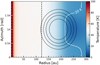 |
Fig. 5 Midplane dust temperature structure of our RADMC-3D model. The black contours indicate the location of the asymmetric dust trap, while the white contour shows where the temperature becomes 20 K. The black dashed line indicates where a temperature of 20 K would be reached assuming a power law for the midplane temperature (van der Marel et al. 2021c). |
4 Discussion
4.1 Observed asymmetries
The observed molecular asymmetries, most notable in the HCN and CS transitions, are striking. As mentioned before, van der Plas et al. (2014) provided two possible explanations for the asymmetries: continuum oversubtraction and freeze-out. Here we explore these possibilities further.
4.1.1 Influence of millimetre-sized dust
Figure 6 presents the deprojected moment-zero maps of the continuum emission and the main CO isotopologues (12CO, 13CO, and C18O), to highlight their azimuthal distributions. None of the isotopologues shows emission at the peak location of the dust trap. As discussed in Sect. 3.4, the CO snowline lies beyond the dust trap, indicating that the lack of emission in the other CO isotopologues must be the result of a continuum oversub-traction. Continuum oversubtraction can be the result of the overestimation of the dust emission that should be removed, as the absorption of dust emission at molecular line frequencies is not taken into account (Boehler et al. 2017, 2021; Weaver et al. 2018). An additional effect follows from the absorption of emission from the far side of the disk by dust particles located in the midplane, which can theoretically result in a depletion of the emission by up to 50% (Isella et al. 2018; Rab et al. 2020; Boehler et al. 2021; Rosotti et al. 2021).
For the other molecules (HCN, CS, and H2CO), continuum oversubtraction can also play a role in the lack of observed emission. However, as these molecules all have higher freeze-out temperatures compared to CO and compared to the estimated peak brightness temperature of the continuum Tdust ≃ 30 K, freeze-out cannot yet be ruled out.
4.1.2 Influence of misaligned warped inner disk
For HCN and CS we propose another scenario to explain the observed asymmetries. As can be seen in the channel maps (Fig. F.1), both molecules show emission enclosing the dust trap, which means that freeze-out at the dust trap alone also cannot explain the observed asymmetry. One possibility left to explore is the influence of the misaligned warped inner disk. As shown by Young et al. (2021), a misaligned warped inner disk can cast shadows on certain parts of the disk, and can subsequently lower the temperature.
Figure 7 shows the HCN and CS moment-zero maps with the scattered light emission (Avenhaus et al. 2014; S. de Regt, priv. comm.) overplotted. The southern shadow is visible in the emission of both HCN and CS, most notably in the HCN emission. The northern shadow, visible in the scattered light emission, also appears to be present in the two channel maps. For both molecules, there is a clear turning point between the bright west side of the disk and the less bright east side of the disk, which appears to occur at the location of the northern shadow.
We propose that the observed asymmetric emission of HCN and CS is the result of the east side of the disk being shadowed by the inner disk, yielding a temperature difference across the disk. This is also supported by the notion that the channel maps display asymmetries in the 4.1–5.1 km s−1 range (see Fig. 8), while the C18O channel map is fully symmetric. From chemical models, we expect HCN and CS to come from the same layer above the midplane (see e.g. Agúndez et al. 2018), explaining why the two molecules would similarly be affected by the misaligned inner disk. The effects of the misalignment are also expected to be visible in the C18O emission (Walsh et al. 2017; Young et al. 2021) as the emission is optically thick, and hence trace the gas temperature. Future work is required to investigate the proper orientation of the inner disk with respect to the other disk and to confirm whether this proposition holds true.
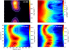 |
Fig. 6 Deprojected moment-zero maps of the continuum and the major CO isotopologues. As in Fig. 1, the 12CO emission is presented using a power-law scaling with a power of 0.5. The white dashed contour lines indicate the location of the continuum emission. |
4.2 The elemental C/O ratio
The ratio between the column densities of CS and SO can be used as a proxy for the volatile C/O ratio (e.g. Le Gal et al. 2019, 2021). For example, Le Gal et al. (2021) derived lower limits on the CS/SO ratio between ~4 and 12 for the disks in the MAPS program. By taking the column density ratio of the CS J = 7−6 transition to the 3σ upper limit for the SO J = 12−01, displayed in Table 1, we obtain CS/SO>1. As we have observations for both CS and HCN, and no observations of other oxygen-bearing species, such as SO, SO2, or NO, this agrees with an expected gas-phase [C]/[O]≳1. To confirm and further explore the C/O ratio, deeper SO observations of brighter lines, for example the J = 53,3−42,2 transition observed in IRS 48 (Booth et al. 2021a) or the J = 77−66 transition observed in HD 100546 (Booth et al. 2023), are required.
4.3 Formation of H2CO
The ratio of the derived total column density of H2CO to the lowest upper limit of CH3OH (using the J = 71,6−70,7 transition) provides insight into the formation of H2CO. Taking the ratio, we find H2CO/CH3OH≳114±14. As expected from the non-detections of CH3OH, H2CO is much more abundant. Taking into account that the molecules share a grain-surface formation route (the hydrogenation of CO), it is very unlikely that the observed H2CO is only thermally desorbed from the ices. This is further supported by the found location of the CO snowline and the low (~30 K) brightness temperature for the continuum emission. As the CO snowline is located beyond the dust trap, we do not expect CO to be frozen out at the grains in the dust trap. This means that H2CO (and CH3OH) cannot actively form on the grains through CO hydrogenation, but could have done so in a previous colder phase, as was found for IRS 48 (van der Marel et al. 2021b) and HD 100546 (Booth et al. 2021b). Furthermore, as we assume the 12CO emission to be optically thick, the kinematic temperature can be approximated to be equal to the brightness temperature, Tkin ~ 40 K (see Sect. 3.4; Garg et al. 2021). As this is lower than the sublimation temperature of H2CO (~66 K; Penteado et al. 2017), thermal desorption of H2CO can be ruled out.
Subsequently, there are two options left to explain the observed H2CO emission: (1) through cold gas-phase neutral-neutral reactions, mainly CH3+O→H2CO+H and CH2+OH→H2CO+H (e.g. Loomis et al. 2015; Terwisscha van Scheltinga et al. 2021), or (2) through non-thermal desorption processes. The found rotational temperature for H2CO of ~20 K hints that the observed emission, assuming that the densities are high enough for LTE, likely originates from the molecular layer (20–50 K), but close to the midplane (10–30 K; e.g. Walsh et al. 2010; Pegues et al. 2020). As most of the H2CO emission is found on the opposite side of the disk, away from the millimetre-sized dust trap, we expect the observed gaseous H2CO emission to mainly have formed through cold gas-phase chemistry. At the location of the dust trap, however, a contribution from non-thermal desorption processes cannot be ruled out. The above analysis agrees with that for TW Hya by Terwisscha van Scheltinga et al. (2021), where gas-phase formation can explain the observed H2CO, but ice-phase formation and contributions in the cold outer disk cannot be ruled out. In addition, Pegues et al. (2020) found H2CO emission to originate from both inside and outside the CO snowline for a small variety of disks, which suggests that H2CO forms through both the gas-and ice-phase formation pathways.
Both proposed options for the observed H2CO emission, gas-phase formation and non-thermal desorption processes, are consistent with the lack of CH3OH. First, CH3OH is known to not form efficiently in the gas-phase and, second, CH3OH fragments during non-thermal desorption processes (Bertin et al. 2016; Cruz-Diaz et al. 2016; Walsh et al. 2018; Santos et al. 2023).
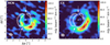 |
Fig. 7 HCN J = 4−3 and CS J = 7−6 moment-zero maps. The white contours show the scattered light emission from the micrometre-sized dust grains, obtained with the NACO instrument in the Ks-band, and the white arrows indicate the location of the shadows. |
 |
Fig. 8 Zoomed-in image of the 4.1–5.1 km s−1 region of the channel maps of C18O J = 3−2 (top), HCN J = 4−3 (middle), and CS J = 7−6 transitions. The C18O channel maps show symmetric emission, while the channel maps of HCN and CS are both clearly asymmetric. The resolving beam is displayed in the lower left and the white star in the centre indicates the inferred location of the host star. The white contours indicate the 3σ and 5σ RMS levels, while the black contours show the 10σ and 15σ RMS levels. |
Column densities (in cm−2) and molecular ratios in the IRS 48 and HD 142527 disks.
4.4 Comparisons with IRS 48
As mentioned before, the differences between the disks of IRS 48 (stellar type A0, L = 17.8 L⊙; Francis & van der Marel 2020) and HD 142527 (stellar type F6, L = 9.9 L⊙; Francis & van der Marel 2020) are remarkable. Not only are different molecules observed in the disks, but the emission morphologies are also strikingly different. In addition, the estimations for both the gas and dust mass are much higher for HD 142527 compared to IRS 48. In the following subsections, we discuss the implications of these differences.
4.4.1 CS and SO
Using the (non-)detections of CS and SO, the elemental C/O ratios in the two disks can be compared. For IRS 48, Booth et al. (2021a) found a CS/SO ratio of ≤0.012 (see Table 2), while for HD 142527 we derived, as discussed in Sect. 4.2, a ratio CS/SO>1. The different ratios can be explained by considering the disks to be either ‘warm’ or ‘cold’ (van der Marel et al. 2021c). The inner cavity walls of the warm disks, such as IRS 48, are irradiated and, subsequently, oxygen-bearing species can be returned to the gas-phase through sublimation of ices. For disks such as HD 142527, which have dust traps at much larger radii, the temperature is too low for the sublimation of these kinds of ices, yielding higher C/O ratios. The location of the dust trap (displayed for both dust traps in Fig. 9) plays a major role in determining whether the temperature at the inner wall is high enough for the sublimation of ices. To elaborate, the IRS 48 dust trap is located at ~60 au, whereas the HD 142527 dust trap is located at ~150 au. The location of the dust trap must thus be taken into account when investigating the influence of the dust trap in the observable chemistry of the disk. While for both disks the dust trap is found to be located inside the CO snowline, sublimation is not observed in HD 142527, suggesting that the temperature might be lower compared to IRS 48. Potentially, the temperature at the cavity wall of IRS 48 is higher compared to that of HD 142527, allowing ices to undergo sublimation. Another possible explanation is that the HD 142527 disk might be less turbulent compared to the IRS 48 disk. As proposed in van der Marel et al. (2021b), icy dust grains end up in the warmer upper layers of the disk at the cavity wall, due to both radial and vertical transportation, allowing for the sublimation of ices. If vertical transportation does not take place, or does take place to a lesser extent in the HD 142527 disk, the grains do not end up in the warmer layers where ice sublimation can take place.
Furthermore, the elemental ratios in the inner disks are also impacted in these disks, affecting the chemical reservoirs available for terrestrial planets. If the sublimation front of the dust trap in a warm disk is located inside the H2O snowline, the inner disk has high gas-phase C/H and O/H ratios. In a cold disk, where the dust trap is located further out, the inner disk will have low gas-phase C/H and O/H ratios. These ratios can be probed with infrared spectroscopy, either from the ground or from space. However, as IRS 48 and HD 142527 are both too bright for the James Webb Space Telescope, observations from, for example, the Herschel-PACS (see e.g. Fedele et al. 2013) and the VLT-CRIRES(+) instruments could be used to probe these ratios. Fedele et al. (2013) presented detections of [O I] tran-sition(s) for both HD 142527 and IRS 48, H2O transitions for HD 142527 and detections of [CII] and CO for IRS 48, while CO was detected in HD 142527 by Brown et al. (2013) using CRIRES. In addition, other carbon-bearing species have not (yet) been observed, potentially hinting at a different C/O ratio in the inner disk of HD 142527 compared to the outer disk. Ground-based observations with CRIRES(+) could provide detections of carbon-bearing species and further constrain elemental ratios in the inner disk. For example, Adams et al. (2019) have detected H2O and OH with CRIRES in the Herbig Ae/Be star HD 101412, while Banzatti et al. (2022) have presented CO-observations in a large sample of disks using both iSHELL on the Infrared Telescope Facility and CRIRES.
These elemental ratios, as mentioned in the Introduction, have implications for the (giant) planets forming in these disks. If a giant planet is accreting its atmosphere in the cavity of a disk such as IRS 48, the atmosphere will have an elemental ratio of C/O<1. On the other hand, a giant planet accreting its atmospheres in a disk like HD 142527 will have an atmospheric elemental ratio of C/O>1.
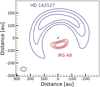 |
Fig. 9 Contour maps of the continuum images for IRS 48 (band 7, in red) and HD 142527 (band 6, in blue). For IRS 48 the contours indicate the 25σ, 75σ, and 150σ levels, while for HD 142527 the 50σ, 150σ and 300σ levels are shown. The IRS 48 continuum emission peaks at ~175 au, whereas the HD 142527 continuum emission peaks at ~60 au. The location of the host star is given by the black star and the resolving beams for the two images are shown in the lower left in their respective colours. |
4.4.2 H2CO and CH3OH
The different formation routes for H2CO in the two disks is also reflected in their H2CO/CH3OH ratios (see Table 2). For HD 142527 we established in Sect. 4.3 that the observed H2CO must be dominantly formed in the gas. Using the ratio of the total derived column density for H2CO (see Sect. 2.5) and the calculated 3σ upper limit for the CH3OH J = 71,6−60,7 transition, we derived H2CO/CH3OH≳114 (see Table 2). For IRS 48, van der Marel et al.(2021b) found a ratio of H2CO/CH3OH~0.2. The higher H2CO/CH3OH ratio thus points to a cold gas-phase formation of H2 CO, whereas a low ratio points towards the grain-surface route, through which both molecules form efficiently. However, the bulk of the H2CO and CH3OH might still be locked up in ices and possibly have a different ratio.
4.4.3 Effect of different gas mass
The difference in the gas mass might also play a role in producing the large differences between observed column densities and ratios (see Table 2). The gas mass of the IRS 48 disk is a factor of ~100 lower compared to that of HD 142527, while the observed abundances of both SO and CH3OH in IRS 48 are a factor of ~100 higher than the estimated lower limits for HD 142527, yielding for both molecules a total difference of a factor ~ 10 000 regarding gas mass and observed abundance. The low gas mass in IRS 48 might result in low column densities of species formed in the gas phase (e.g. CN and C2H; Leemker et al. 2023), such that only those sublimating from the ices can be easily observed. The current observations of HD 142527 have not reached high enough sensitivity to detect gas-phase species like SO that could be located at its dust trap.
4.5 Comparisons with HD 100546
In addition to being observed in IRS 48, SO, H2CO, and CH3OH have also been observed in the disk of HD 100546 (Booth et al. 2021b, 2023), a Herbig Be (Vioque et al. 2018) disk with two symmetric dust rings. The inner dust ring of HD 100546 extends between ~20 and 40 au, while the second ring is centred at ~200 au (Fedele et al. 2021). The emission of SO, H2CO, and CH3OH has a central compact emission component and an outer ring, which is well detected for both SO and H2CO. For the inner component, the emission is thought to be the result of thermal sublimation at the inner dust cavity edge, as it is for IRS 48; instead, for the outer ring the emission might be the result of other desorption processes. As the radial column densities of SO and CH3OH at the location of the outer dust ring are of the same order of magnitude as our 3σ upper limits, the outer ring of HD 100546 might closely resemble the asymmetric dust trap of HD 142527. However, the outer ring of HD 100546 contains significantly less dust mass compared the dust trap of HD 142527. Another difference is that we have not (yet) reached the sensitivity in the HD 142527 observations to detect the products of non-thermal desorption processes. Deeper observations focusing on SO and CH3OH are necessary to investigate the possibility of observing products of non-thermal desorption processes in the HD 142527 disk.
5 Summary
In this work, we have investigated the chemistry of the HD 142527 disk using ALMA archival data. We summarise our main conclusions here:
We report the first ALMA detections of [CI], 13C18O,DCO+, and H2CO transitions in the HD 142527 planet-forming disk. Additionally, we report observations of the HCO+ J =8−7 and CS J = 10−9 transitions in this disk;
The observed molecular asymmetries are thought to be partially caused by continuum oversubtraction. Additionally, we propose that shadowing of the misaligned, warped inner disk on the eastern side of the disk causes the asymmetries observed in the HCN and CS emission;
The dust and gas mass were recalculated, yielding values of Mdust = 1.5× 10⁻³ M⊙ and Mgas = 1.6× 10⁻² M⊙, respectively. These estimates yield a gas-to-dust ratio of ~11;
Based on our observations of 13C18O and DCO+, we expect the CO snowline to be located beyond the dust trap at a location of ~300 au, which is supported by our RADMC-3D model;
Using our detection of the CS J =7−6 transition and the 3σ upper limit on the SO J = 12−01 transition, we estimate C/O>1. The higher ratio is likely due to oxygen-bearing species being frozen out on the dust trap, and is higher than that found for IRS 48, where oxygen-bearing species are returned to the gas-phase through sublimation;
Finally, the observed H2CO is expected to come from the molecular layer above the midplane. Furthermore, we propose that the observed H2CO is mainly formed in the gas-phase, but contributions from ice-phase formation pathways and non-thermal desorption processes cannot be ruled out. By taking the ratio of the found H2CO column density and the 3σ upper limit for CH3OH, we find a H2CO/CH3OH ratio of ~ 114. The ratio is significantly higher than that found for IRS 48 (~0.2). In IRS 48, both H2CO and CH3OH are observed through the sublimation of ices, yielding the lower ratio and further confirming that the observed H2CO must have formed primarily through gas-phase reactions.
The observed molecular content of the HD 142527 disk is clearly different from that of IRS 48 and HD 100546. In particular, in HD 142527 all of the molecules, aside from the CO isotopo-logues, peak in the region of the disk where millimetre-sized dust is absent, which is the opposite of what was observed in IRS 48. Deeper observations targeting SO and CH3OH are needed to detect or obtain meaningful upper limits on their relative abundances in order to understand the dominant chemical process(es) occurring in the HD 142527 disk compared to that in IRS 48. The chemical differences between IRS 48 and HD 142527 might arise from the different radial distances of the dust traps with respect to the host stars, from shadowing due to a misaligned inner disk, and/or from a different degree of turbulence in the azimuthal dust traps.
Acknowledgements
We acknowledge assistance from Allegro, the European ALMA Regional Centre node in the Netherlands. Astrochemistry in Leiden is supported by funding from the European Research Council (ERC) under the European Union’s Horizon 2020 research and innovation programme (grant agreement No. 101019751 MOLDISK) and by the Netherlands Research School for Astronomy (NOVA). This work makes use of the following ALMA data: ADS/JAO.ALMA#2011.0.00318.S, ADS/JAO.ALMA#2011.0.00465.S, ADS/JAO.ALMA#2012.1.00613.S, ADS/JAO.ALMA#2013.1.00305.S, ADS/JAO.ALMA#2015.1.00614.S, ADS/JAO.ALMA#2015.1.00805.S, ADS/JAO.ALMA#2015.1.01137.S. ALMA is a partnership of ESO (representing its member states), NSF (USA) and NINS (Japan), together with NRC (Canada), MOST and ASIAA (Taiwan), and KASI (Republic of Korea), in cooperation with the Republic of Chile. The Joint ALMA Observatory is operated by ESO, AUI/NRAO and NAOJ. This work has used the following additional software packages that have not been referred to in the main text: Astropy, IPython, Jupyter, Matplotlib, NumPy, pandas and SciPy (Astropy Collaboration 2022; Pérez & Granger 2007; Kluyver et al. 2016; Hunter 2007; Harris et al. 2020; pandas development team 2020; Wes McKinney 2010; Virtanen et al. 2020).
Appendix A Observed molecules
Datasets used throughout this work.
Appendix B Additional moment-zero maps
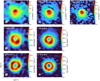 |
Fig. B.1 Moment-zero maps of the observed CO isotopologue transitions. From top to bottom are shown the 12CO, 13CO, and C18O isotopologues, while from left to right are shown the J=2-1, J=3-2, and J=6-5 transitions. The beams are displayed in the lowerleft, while the approximate location of the host star is given by the white star. The 12CO colour maps are displayed using a power-law scaling with an exponent of 0.5. |
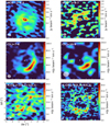 |
Fig. B.2 Moment-zero maps of the observed HCO+ (top row), CS (middle row), and H2CO (bottom row) transitions. The beams are displayed in the lower left and the white star in the centre indicates the inferred location of the host star. The HCO+ colour-maps are displayed using a power-law scaling with an exponent of 0.5. |
Appendix C GoFish spectra
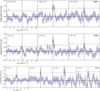 |
Fig. C.1 Spectra acquired from different radial regimes with GoFish. The radial regimes for each spectrum are indicated in the top left. From top to bottom are shown DCO+ J=4-3, H2CO J=42,3-32,2, and H2CO J=42,2-32,1. The horizontal red dashed line in each spectrum indicates the 3σ RMS level, while the vertical black dashed line indicates the systemic velocity of 3.6 km s−1. |
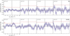 |
Fig. C.2 Same as Figure C.1, but for the non-detections of the SO J=12-01 (top panel) and the CH3OH J=71,6-70,7 (bottom panel) transitions. |
Appendix D Rotational diagram analysis: Posterior distributions
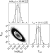 |
Fig. D.1 Posterior distributions of the rotational diagram analysis for H2CO. |
Appendix E RADMC-3D Model
The RADMC-3D model was visually fitted to both the dered-dened SED (obtained from Verhoeff et al. 2011), using AV=0.3 mag (Francis & van der Marel 2020) and the ALMA continuum radial profile. For the model we used the standard DIANA opacities (Woitke et al. 2016), implemented using Op Tool (Dominik et al. 2021). We used two different dust size distributions (both with 100 sample sizes), one for the small grains with sizes from 0.005 µm to 1 µm and one for the large grains with sizes from 0.005 µm to 1000 µm. These size distributions were used for both the inner and the outer disk.
We modelled the inner disk by assuming an exponentially tapered surface density,
![Mathematical equation: ${\rm{\Sigma }}\left( R \right) = {{\rm{\Sigma }}_c}\,{\left( {{R \over {{R_{{\rm{c,ID}}}}}}} \right)^\gamma }\,\exp \,\left[ { - {{\left( {{R \over {{R_{{\rm{c,ID}}}}}}} \right)}^{2 - \gamma }}} \right],$](/articles/aa/full_html/2023/07/aa46272-23/aa46272-23-eq19.png) (E.1)
(E.1)
where Rc,ID=40 au and γ=1 were used. In addition, the inner disk starts at the dust sublimation radius, estimated to be located at Rsub=0.07 (L/L⊙)1/2 ≃0.22 au, assuming a sublimation radius of 1500 K (Dullemond et al. 2001). The outer disk was modelled by a Gaussian in both the radial and azimuthal directions to create the asymmetric ring. The median for the azimuthal Gaussian was set to π and we used a standard deviation of 0.18π, yielding the arbitrary orientation, but similar shape, of the model asymmetry displayed in the bottom left of Figure E.2. Additionally, the cavity, which is fully depleted from both grain distributions, extends from 40 to 100 au.
Both inner and outer disks were given different vertical structures, described with the following equation:
 (E.2)
(E.2)
For the inner disk we used hc=0.2, Rc=Rc,ID and ψ=0.05, while for the outer disk we used hc=0.35, Rc=150, and ψ=0.2. Furthermore, we took for the inner and outer disk two separate fractions of large grains, 50% and 85%, respectively. For both the inner and outer disk we set the large grain settling factor to χ=0.1.
Furthermore, in order to properly fit the radial profile we had to increase the dust mass to Mdust=7.5×10⁻³ M⊙. This is about five times larger than our estimate in Sect. 3.2. The higher dust mass is likely partially linked to the used opacities, but also provides further hints that the continuum emission is optically thick and our dust mass estimate is a lower limit.
The resulting fit is displayed in Figure E.2; the continuum and model images are on the left, and the radial profile and SED are on the right. Overall the model fits reasonably well to both the radial profile and the SED, only slightly overproducing the inner disk. The fit, however, is good enough for the aims of the model, which is to provide a second check of the approximate location of the CO snowline.
Additionally, for comparison with the estimated location of the snowline in van der Marel (2023), the white dashed line displays the 20 K line when assuming a power-law midplane temperature structure (Chiang & Goldreich 1997; Dullemond et al. 2001):
 (E.3)
(E.3)
Here, following van der Marel et al. (2021c), we take ϕ = 0.02. As can be seen, the white dashed line is well within the dust trap, showing that a simple power law for the midplane temperature does not yield the right location of the CO snowline for the HD 142527 disk. This is very likely due to the large cavity, indicating that temperature structure, and hence the snowline locations of transition disks with large cavities, cannot be determined by a power-law approximation of the midplane temperature.
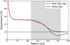 |
Fig. E.1 Dust midplane temperature at the peak location of the model dust trap (blue line) and the other side of the disk (red line). The horizontal dashed black line indicates a temperature of 20 K. The grey shaded area displays the outermost contour levels of the modelled dust trap in Figure 5. |
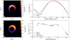 |
Fig. E.2 Resulting RADMC-3D fit to the radial profile (top right) and SED (bottom right). The continuum image is shown at the top left, while the model image is shown at the bottom left. For the radial profile and the SED the observations are shown in black, while the model is shown in red. The green line within the SED displays high-resolution Spitzer observations (Bouwman et al. 2004). |
Appendix F Full channel maps
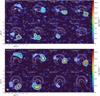 |
Fig. F.1 Channels maps of the HCN J=4-3 (top) and CS J=7-6 (bottom) transitions. The resolving beam is displayed in the lower left and the white star in the centre gives the approximate location of the host star. The white contours indicate the 3σ and 5σ RMS levels, while the black contours show the 10σ and 15σ RMS levels. The location of the continuum emission is in each map indicated by the white dashed contours. |
References
- Adams, S. C., Ádámkovics, M., Carr, J. S., Najita, J. R., & Brittain, S. D. 2019, ApJ, 871, 173 [NASA ADS] [CrossRef] [Google Scholar]
- Agúndez, M., Roueff, E., Le Petit, F., & Le Bourlot, J. 2018, A&A, 616, A19 [Google Scholar]
- Andrews, S. M., Huang, J., Pérez, L. M., et al. 2018, ApJ, 869, L41 [NASA ADS] [CrossRef] [Google Scholar]
- Ansdell, M., Williams, J. P., van der Marel, N., et al. 2016, ApJ, 828, 46 [Google Scholar]
- Astropy Collaboration (Price-Whelan, A. M., et al..) 2022, ApJ, 935, 167 [NASA ADS] [CrossRef] [Google Scholar]
- Avenhaus, H., Quanz, S. P., Schmid, H. M., et al. 2014, ApJ, 781, 87 [Google Scholar]
- Avenhaus, H., Quanz, S. P., Schmid, H. M., et al. 2017, AJ, 154, 33 [Google Scholar]
- Balmer, W. O., Follette, K. B., Close, L. M., et al. 2022, AJ, 164, 29 [NASA ADS] [CrossRef] [Google Scholar]
- Banzatti, A., Pascucci, I., Bosman, A. D., et al. 2020, ApJ, 903, 124 [NASA ADS] [CrossRef] [Google Scholar]
- Banzatti, A., Abernathy, K. M., Brittain, S., et al. 2022, AJ, 163, 174 [NASA ADS] [CrossRef] [Google Scholar]
- Beckwith, S. V. W., Sargent, A. I., Chini, R. S., & Guesten, R. 1990, AJ, 99, 924 [Google Scholar]
- Bergin, E. A., & Williams, J. P. 2017, Astrophys. Space Sci. Lib., 445, 1 [NASA ADS] [CrossRef] [Google Scholar]
- Bertin, M., Romanzin, C., Doronin, M., et al. 2016, ApJ, 817, L12 [NASA ADS] [CrossRef] [Google Scholar]
- Biller, B., Lacour, S., Juhász, A., et al. 2012, ApJ, 753, L38 [Google Scholar]
- Boehler, Y., Weaver, E., Isella, A., et al. 2017, ApJ, 840, 60 [Google Scholar]
- Boehler, Y., Ménard, F., Robert, C. M. T., et al. 2021, A&A, 650, A59 [NASA ADS] [CrossRef] [EDP Sciences] [Google Scholar]
- Bohn, A. J., Benisty, M., Perraut, K., et al. 2022, A&A, 658, A183 [NASA ADS] [CrossRef] [EDP Sciences] [Google Scholar]
- Booth, R. A., Clarke, C. J., Madhusudhan, N., & Ilee, J. D. 2017, MNRAS, 469, 3994 [Google Scholar]
- Booth, A. S., Walsh, C., Ilee, J. D., et al. 2019, ApJ, 882, L31 [Google Scholar]
- Booth, A. S., van der Marel, N., Leemker, M., van Dishoeck, E. F., & Ohashi, S. 2021a, A&A, 651, A6 [NASA ADS] [CrossRef] [EDP Sciences] [Google Scholar]
- Booth, A. S., Walsh, C., Terwisscha van Scheltinga, J., et al. 2021b, Nat. Astron., 5, 684 [NASA ADS] [CrossRef] [Google Scholar]
- Booth, A. S., Ilee, J. D., Walsh, C., et al. 2023, A&A, 669, A53 [Google Scholar]
- Bosman, A. D., & Banzatti, A. 2019, A&A, 632, A10 [Google Scholar]
- Bouwman, J., Dominik, C., Dullemond, C. P., et al. 2004, The mineralogy of proto-planetary disks surrounding Herbig Ae/Be stars, Spitzer Proposal, 3470 [Google Scholar]
- Brown, J. M., Pontoppidan, K. M., van Dishoeck, E. F., et al. 2013, ApJ, 770, 94 [NASA ADS] [CrossRef] [Google Scholar]
- Bruderer, S., van der Marel, N., van Dishoeck, E. F., & van Kempen, T. A. 2014, A&A, 562, A26 [NASA ADS] [CrossRef] [EDP Sciences] [Google Scholar]
- Brunken, N. G. C., Booth, A. S., Leemker, M., et al. 2022, A&A, 659, A29 [NASA ADS] [CrossRef] [EDP Sciences] [Google Scholar]
- Calahan, J. K., Bergin, E., Zhang, K., et al. 2021, ApJ, 908, 8 [NASA ADS] [CrossRef] [Google Scholar]
- Canovas, H., Ménard, F., Hales, A., et al. 2013, A&A, 556, A123 [NASA ADS] [CrossRef] [EDP Sciences] [Google Scholar]
- Carney, M. T., Fedele, D., Hogerheijde, M. R., et al. 2018, A&A, 614, A106 [NASA ADS] [CrossRef] [EDP Sciences] [Google Scholar]
- Carney, M. T., Hogerheijde, M. R., Guzmán, V. V., et al. 2019, A&A, 623, A124 [NASA ADS] [CrossRef] [EDP Sciences] [Google Scholar]
- Casassus, S., van der Plas, G. M., Perez, S., et al. 2013, Nature, 493, 191 [Google Scholar]
- Casassus, S., Marino, S., Pérez, S., et al. 2015, ApJ, 811, 92 [Google Scholar]
- Cazzoletti, P., Manara, C. F., Liu, H. B., et al. 2019, A&A, 626, A11 [NASA ADS] [CrossRef] [EDP Sciences] [Google Scholar]
- Chiang, E. I., & Goldreich, P. 1997, ApJ, 490, 368 [Google Scholar]
- Cleeves, L. I. 2016, ApJ, 816, L21 [NASA ADS] [CrossRef] [Google Scholar]
- Cleeves, L. I., Loomis, R. A., Teague, R., et al. 2021, ApJ, 911, 29 [NASA ADS] [CrossRef] [Google Scholar]
- Cruz-Diaz, G. A., Martín-Doménech, R., Muñoz Caro, G. M., & Chen, Y. J. 2016, A&A, 592, A68 [NASA ADS] [CrossRef] [EDP Sciences] [Google Scholar]
- Dominik, C., Min, M., & Tazaki, R. 2021, Astrophysics Source Code Library [record ascl:2104.010] [Google Scholar]
- Dullemond, C. P., Dominik, C., & Natta, A. 2001, ApJ, 560, 957 [NASA ADS] [CrossRef] [Google Scholar]
- Dullemond, C. P., Juhasz, A., Pohl, A., et al. 2012, Astrophysics Source Code Library [record ascl:1202.015] [Google Scholar]
- Eistrup, C. 2023, ACS Earth Space Chem., 7, 260 [NASA ADS] [CrossRef] [Google Scholar]
- Eistrup, C., Walsh, C., & van Dishoeck, E. F. 2018, A&A, 613, A14 [NASA ADS] [CrossRef] [EDP Sciences] [Google Scholar]
- Facchini, S., Birnstiel, T., Bruderer, S., & van Dishoeck, E. F. 2017, A&A, 605, A16 [NASA ADS] [CrossRef] [EDP Sciences] [Google Scholar]
- Facchini, S., Teague, R., Bae, J., et al. 2021, AJ, 162, 99 [NASA ADS] [CrossRef] [Google Scholar]
- Fairlamb, J. R., Oudmaijer, R. D., Mendigutía, I., Ilee, J. D., & van den Ancker, M. E. 2015, MNRAS, 453, 976 [Google Scholar]
- Fedele, D., Bruderer, S., van Dishoeck, E. F., et al. 2013, A&A, 559, A77 [CrossRef] [EDP Sciences] [Google Scholar]
- Fedele, D., Toci, C., Maud, L., & Lodato, G. 2021, A&A, 651, A90 [NASA ADS] [CrossRef] [EDP Sciences] [Google Scholar]
- Foreman-Mackey, D., Hogg, D. W., Lang, D., & Goodman, J. 2013, PASP, 125, 306 [Google Scholar]
- Francis, L., & van der Marel, N. 2020, ApJ, 892, 111 [Google Scholar]
- Fuchs, G. W., Cuppen, H. M., Ioppolo, S., et al. 2009, A&A, 505, 629 [NASA ADS] [CrossRef] [EDP Sciences] [Google Scholar]
- Fukagawa, M., Tamura, M., Itoh, Y., et al. 2006, ApJ, 636, L153 [Google Scholar]
- Gaia Collaboration (Brown, A. G. A., et al..) 2018, A&A, 616, A1 [NASA ADS] [CrossRef] [EDP Sciences] [Google Scholar]
- Garg, H., Pinte, C., Christiaens, V., et al. 2021, MNRAS, 504, 782 [Google Scholar]
- Goldsmith, P. F., & Langer, W. D. 1999, ApJ, 517, 209 [Google Scholar]
- Harris, C. R., Millman, K. J., van der Walt, S. J., et al. 2020, Nature, 585, 357 [NASA ADS] [CrossRef] [Google Scholar]
- Hildebrand, R. H. 1983, QJRAS, 24, 267 [NASA ADS] [Google Scholar]
- Huang, J., Öberg, K. I., Qi, C., et al. 2017, ApJ, 835, 231 [Google Scholar]
- Hunter, J. D. 2007, Comput. Sci. Eng., 9, 90 [NASA ADS] [CrossRef] [Google Scholar]
- Isella, A., Huang, J., Andrews, S. M., et al. 2018, ApJ, 869, L49 [NASA ADS] [CrossRef] [Google Scholar]
- Kluyver, T., Ragan-Kelley, B., Pérez, F., et al. 2016, in Positioning and Power in Academic Publishing: Players, Agents and Agendas, eds. F. Loizides, & B. Schmidt (IOS Press), 87 [Google Scholar]
- Krijt, S., Schwarz, K. R., Bergin, E. A., & Ciesla, F. J. 2018, ApJ, 864, 78 [Google Scholar]
- Krijt, S., Bosman, A. D., Zhang, K., et al. 2020, ApJ, 899, 134 [NASA ADS] [CrossRef] [Google Scholar]
- Lacour, S., Biller, B., Cheetham, A., et al. 2016, A&A, 590, A90 [NASA ADS] [CrossRef] [EDP Sciences] [Google Scholar]
- Leemker, M., Booth, A. S., van Dishoeck, E. F., et al. 2022, A&A, 663, A23 [NASA ADS] [CrossRef] [EDP Sciences] [Google Scholar]
- Leemker, M., Booth, A. S., van Dishoeck, E. F., et al. 2023, A&A, 673, A7 [NASA ADS] [CrossRef] [EDP Sciences] [Google Scholar]
- Le Gal, R., Brady, M. T., Öberg, K. I., Roueff, E., & Le Petit, F. 2019, ApJ, 886, 86 [NASA ADS] [CrossRef] [Google Scholar]
- Le Gal, R., Öberg, K. I., Teague, R., et al. 2021, ApJS, 257, 12 [NASA ADS] [CrossRef] [Google Scholar]
- Long, F., Pinilla, P., Herczeg, G. J., et al. 2018, ApJ, 869, 17 [Google Scholar]
- Loomis, R. A., Cleeves, L. I., Öberg, K. I., Guzman, V. V., & Andrews, S. M. 2015, ApJ, 809, L25 [Google Scholar]
- Loomis, R. A., Öberg, K. I., Andrews, S. M., et al. 2020, ApJ, 893, 101 [Google Scholar]
- Marino, S., Perez, S., & Casassus, S. 2015, ApJ, 798, L44 [Google Scholar]
- Mathews, G. S., Klaassen, P. D., Juhász, A., et al. 2013, A&A, 557, A132 [NASA ADS] [CrossRef] [EDP Sciences] [Google Scholar]
- McClure, M. K., Dominik, C., & Kama, M. 2020, A&A, 642, A15 [NASA ADS] [CrossRef] [EDP Sciences] [Google Scholar]
- McMullin, J. P., Waters, B., Schiebel, D., Young, W., & Golap, K. 2007, ASP Conf. Ser., 376, 127 [Google Scholar]
- Milam, S. N., Savage, C., Brewster, M. A., Ziurys, L. M., & Wyckoff, S. 2005, ApJ, 634, 1126 [Google Scholar]
- Miley, J. M., Panić, O., Booth, R. A., et al. 2021, MNRAS, 500, 4658 [Google Scholar]
- Millar, T. J., Bennett, A., & Herbst, E. 1989, ApJ, 340, 906 [NASA ADS] [CrossRef] [Google Scholar]
- Miyake, K., & Nakagawa, Y. 1993, Icarus, 106, 20 [NASA ADS] [CrossRef] [Google Scholar]
- Müller, H. S. P., Thorwirth, S., Roth, D. A., & Winnewisser, G. 2001, A&A, 370, L49 [Google Scholar]
- Müller, H. S. P., Schlöder, F., Stutzki, J., & Winnewisser, G. 2005, J. Mol. Struct., 742, 215 [Google Scholar]
- Öberg, K. I., & Bergin, E. A. 2021, Phys. Rep., 893, 1 [Google Scholar]
- Öberg, K. I., Murray-Clay, R., & Bergin, E. A. 2011, ApJ, 743, L16 [Google Scholar]
- Öberg, K. I., Furuya, K., Loomis, R., et al. 2015, ApJ, 810, 112 [Google Scholar]
- Öberg, K. I., Cleeves, L. I., Bergner, J. B., et al. 2021a, AJ, 161, 38 [Google Scholar]
- Öberg, K. I., Guzmán, V. V., Walsh, C., et al. 2021b, ApJS, 257, 1 [CrossRef] [Google Scholar]
- Pacetti, E., Turrini, D., Schisano, E., et al. 2022, ApJ, 937, 36 [NASA ADS] [CrossRef] [Google Scholar]
- pandas development team 2020, https://doi.org/10.5281/zenodo.3509134 [Google Scholar]
- Pegues, J., Öberg, K. I., Bergner, J. B., et al. 2020, ApJ, 890, 142 [Google Scholar]
- Penteado, E. M., Walsh, C., & Cuppen, H. M. 2017, ApJ, 844, 71 [Google Scholar]
- Pérez, F., & Granger, B. E. 2007, Comput. Sci. Eng., 9, 21 [Google Scholar]
- Qi, C., Öberg, K. I., & Wilner, D. J. 2013a, ApJ, 765, 34 [NASA ADS] [CrossRef] [Google Scholar]
- Qi, C., Öberg, K. I., Wilner, D. J., et al. 2013b, Science, 341, 630 [Google Scholar]
- Qi, C., Öberg, K. I., Espaillat, C. C., et al. 2019, ApJ, 882, 160 [Google Scholar]
- Rab, C., Kamp, I., Dominik, C., et al. 2020, A&A, 642, A165 [EDP Sciences] [Google Scholar]
- Roberts, H., & Millar, T. J. 2000, A&A, 361, 388 [NASA ADS] [Google Scholar]
- Rosotti, G. P., Ilee, J. D., Facchini, S., et al. 2021, MNRAS, 501, 3427 [Google Scholar]
- Roueff, E., Gerin, M., Lis, D. C., et al. 2013, J. Phys. Chem. A, 117, 9959 [Google Scholar]
- Salinas, V. N., Hogerheijde, M. R., Mathews, G. S., et al. 2017, A&A, 606, A125 [NASA ADS] [CrossRef] [EDP Sciences] [Google Scholar]
- Santos, J. C., Chuang, K. J., Schrauwen, J. G. M., et al. 2023, A&A, 672, A112 [NASA ADS] [CrossRef] [EDP Sciences] [Google Scholar]
- Stapper, L. M., Hogerheijde, M. R., van Dishoeck, E. F., & Mentel, R. 2022, A&A, 658, A112 [NASA ADS] [CrossRef] [EDP Sciences] [Google Scholar]
- Sturm, J. A., Booth, A. S., McClure, M. K., Leemker, M., & van Dishoeck, E. F. 2023, A&A, 670, A12 [NASA ADS] [CrossRef] [EDP Sciences] [Google Scholar]
- Teague, R. 2019, J. Open Source Softw., 4, 1632 [NASA ADS] [CrossRef] [Google Scholar]
- Terwisscha van Scheltinga, J., Hogerheijde, M. R., Cleeves, L. I., et al. 2021, ApJ, 906, 111 [Google Scholar]
- van der Marel, N. 2023, EPJ Plus, 138, 225 [NASA ADS] [Google Scholar]
- van der Marel, N., van Dishoeck, E. F., Bruderer, S., et al. 2013, Science, 340, 1199 [Google Scholar]
- van der Marel, N., van Dishoeck, E. F., Bruderer, S., et al. 2016, A&A, 585, A58 [NASA ADS] [CrossRef] [EDP Sciences] [Google Scholar]
- van der Marel, N., Birnstiel, T., Garufi, A., et al. 2021a, AJ, 161, 33 [Google Scholar]
- van der Marel, N., Booth, A. S., Leemker, M., van Dishoeck, E. F., & Ohashi, S. 2021b, A&A, 651, A5 [Google Scholar]
- van der Marel, N., Bosman, A. D., Krijt, S., Mulders, G. D., & Bergner, J. B. 2021c, A&A, 653, A9 [NASA ADS] [CrossRef] [EDP Sciences] [Google Scholar]
- van der Plas, G., Casassus, S., Ménard, F., et al. 2014, ApJ, 792, L25 [Google Scholar]
- van’t Hoff, M. L. R., Walsh, C., Kama, M., Facchini, S., & van Dishoeck, E. F. 2017, A&A, 599, A101 [Google Scholar]
- Verhoeff, A. P., Min, M., Pantin, E., et al. 2011, A&A, 528, A91 [NASA ADS] [CrossRef] [EDP Sciences] [Google Scholar]
- Vioque, M., Oudmaijer, R. D., Baines, D., Mendigutía, I., & Pérez-Martínez, R. 2018, A&A, 620, A128 [NASA ADS] [CrossRef] [EDP Sciences] [Google Scholar]
- Virtanen, P., Gommers, R., Oliphant, T. E., et al. 2020, Nat. Methods, 17, 261 [Google Scholar]
- Walsh, C., Millar, T. J., & Nomura, H. 2010, ApJ, 722, 1607 [Google Scholar]
- Walsh, C., Daley, C., Facchini, S., & Juhász, A. 2017, A&A, 607, A114 [NASA ADS] [CrossRef] [EDP Sciences] [Google Scholar]
- Walsh, C., Vissapragada, S., & McGee, H. 2018, IAU Symp., 332, 395 [NASA ADS] [Google Scholar]
- Watanabe, N., & Kouchi, A. 2002, ApJ, 571, L173 [Google Scholar]
- Weaver, E., Isella, A., & Boehler, Y. 2018, ApJ, 853, 113 [Google Scholar]
- Wes McKinney 2010, in Proceedings of the 9th Python in Science Conference, eds. S. van der Walt & J. Millman, 56 [Google Scholar]
- Wilson, T. L. 1999, Rep. Progr. Phys., 62, 143 [CrossRef] [Google Scholar]
- Woitke, P., Min, M., Pinte, C., et al. 2016, A&A, 586, A103 [NASA ADS] [CrossRef] [EDP Sciences] [Google Scholar]
- Wölfer, L., Facchini, S., van der Marel, N., et al. 2022, A&A, 670, A154 [Google Scholar]
- Wootten, A. 1987, Astrochemistry, 120, 311 [NASA ADS] [CrossRef] [Google Scholar]
- Yen, H.-W., Koch, P. M., Liu, H. B., et al. 2016, ApJ, 832, 204 [NASA ADS] [CrossRef] [Google Scholar]
- Young, A. K., Alexander, R., Walsh, C., et al. 2021, MNRAS, 505, 4821 [NASA ADS] [CrossRef] [Google Scholar]
- Zhang, K., Bergin, E. A., Schwarz, K., Krijt, S., & Ciesla, F. 2019, ApJ, 883, 98 [Google Scholar]
- Zhang, K., Bosman, A. D., & Bergin, E. A. 2020, ApJ, 891, L16 [NASA ADS] [CrossRef] [Google Scholar]
- Zhang, K., Booth, A. S., Law, C. J., et al. 2021, ApJS, 257, 5 [NASA ADS] [CrossRef] [Google Scholar]
All Tables
Column densities (in cm−2) and molecular ratios in the IRS 48 and HD 142527 disks.
All Figures
|
Fig. 1 Moment-zero maps of the continuum (upper left) and the majority of the detected molecules. The beams are indicated in the lower left and the white star in the centre shows the inferred location of the host star based on the position of the inner disk. The 12CO and HCO+ colour maps are displayed using a power-law scaling with power 0.5. |
| In the text | |
|
Fig. 2 Moment-zero maps of the [C I] 3P1−3P0 transition. From left to right are shown the three execution blocks, the higher angular resolution observations from 19 May 2016, and the other two observations from 23 May 2016. The beams are indicated in the lower left, the white star in the centre shows the inferred location of the host star, and the white dashed contours indicate the location of the continuum emission. |
| In the text | |
|
Fig. 3 Results of the rotational diagram analysis for H2CO. The triangles display the acquired column densities for the non-detected lines, which have not been taken into account during the analysis. Furthermore, the faint, red lines are solutions randomly sampled from the posterior distributions. |
| In the text | |
|
Fig. 4 Azimuthally averaged deprojected radial profiles of 13C18O (in blue) and DCO+ (in red), shown together with the continuum emission (black profile). The shaded areas are the errors on the profiles. The two horizontal bars in the top right indicate the size of the minor axis for 13C18O (blue) and DCO+ (red). |
| In the text | |
|
Fig. 5 Midplane dust temperature structure of our RADMC-3D model. The black contours indicate the location of the asymmetric dust trap, while the white contour shows where the temperature becomes 20 K. The black dashed line indicates where a temperature of 20 K would be reached assuming a power law for the midplane temperature (van der Marel et al. 2021c). |
| In the text | |
|
Fig. 6 Deprojected moment-zero maps of the continuum and the major CO isotopologues. As in Fig. 1, the 12CO emission is presented using a power-law scaling with a power of 0.5. The white dashed contour lines indicate the location of the continuum emission. |
| In the text | |
|
Fig. 7 HCN J = 4−3 and CS J = 7−6 moment-zero maps. The white contours show the scattered light emission from the micrometre-sized dust grains, obtained with the NACO instrument in the Ks-band, and the white arrows indicate the location of the shadows. |
| In the text | |
|
Fig. 8 Zoomed-in image of the 4.1–5.1 km s−1 region of the channel maps of C18O J = 3−2 (top), HCN J = 4−3 (middle), and CS J = 7−6 transitions. The C18O channel maps show symmetric emission, while the channel maps of HCN and CS are both clearly asymmetric. The resolving beam is displayed in the lower left and the white star in the centre indicates the inferred location of the host star. The white contours indicate the 3σ and 5σ RMS levels, while the black contours show the 10σ and 15σ RMS levels. |
| In the text | |
|
Fig. 9 Contour maps of the continuum images for IRS 48 (band 7, in red) and HD 142527 (band 6, in blue). For IRS 48 the contours indicate the 25σ, 75σ, and 150σ levels, while for HD 142527 the 50σ, 150σ and 300σ levels are shown. The IRS 48 continuum emission peaks at ~175 au, whereas the HD 142527 continuum emission peaks at ~60 au. The location of the host star is given by the black star and the resolving beams for the two images are shown in the lower left in their respective colours. |
| In the text | |
|
Fig. B.1 Moment-zero maps of the observed CO isotopologue transitions. From top to bottom are shown the 12CO, 13CO, and C18O isotopologues, while from left to right are shown the J=2-1, J=3-2, and J=6-5 transitions. The beams are displayed in the lowerleft, while the approximate location of the host star is given by the white star. The 12CO colour maps are displayed using a power-law scaling with an exponent of 0.5. |
| In the text | |
|
Fig. B.2 Moment-zero maps of the observed HCO+ (top row), CS (middle row), and H2CO (bottom row) transitions. The beams are displayed in the lower left and the white star in the centre indicates the inferred location of the host star. The HCO+ colour-maps are displayed using a power-law scaling with an exponent of 0.5. |
| In the text | |
|
Fig. C.1 Spectra acquired from different radial regimes with GoFish. The radial regimes for each spectrum are indicated in the top left. From top to bottom are shown DCO+ J=4-3, H2CO J=42,3-32,2, and H2CO J=42,2-32,1. The horizontal red dashed line in each spectrum indicates the 3σ RMS level, while the vertical black dashed line indicates the systemic velocity of 3.6 km s−1. |
| In the text | |
|
Fig. C.2 Same as Figure C.1, but for the non-detections of the SO J=12-01 (top panel) and the CH3OH J=71,6-70,7 (bottom panel) transitions. |
| In the text | |
|
Fig. D.1 Posterior distributions of the rotational diagram analysis for H2CO. |
| In the text | |
|
Fig. E.1 Dust midplane temperature at the peak location of the model dust trap (blue line) and the other side of the disk (red line). The horizontal dashed black line indicates a temperature of 20 K. The grey shaded area displays the outermost contour levels of the modelled dust trap in Figure 5. |
| In the text | |
|
Fig. E.2 Resulting RADMC-3D fit to the radial profile (top right) and SED (bottom right). The continuum image is shown at the top left, while the model image is shown at the bottom left. For the radial profile and the SED the observations are shown in black, while the model is shown in red. The green line within the SED displays high-resolution Spitzer observations (Bouwman et al. 2004). |
| In the text | |
|
Fig. F.1 Channels maps of the HCN J=4-3 (top) and CS J=7-6 (bottom) transitions. The resolving beam is displayed in the lower left and the white star in the centre gives the approximate location of the host star. The white contours indicate the 3σ and 5σ RMS levels, while the black contours show the 10σ and 15σ RMS levels. The location of the continuum emission is in each map indicated by the white dashed contours. |
| In the text | |
Current usage metrics show cumulative count of Article Views (full-text article views including HTML views, PDF and ePub downloads, according to the available data) and Abstracts Views on Vision4Press platform.
Data correspond to usage on the plateform after 2015. The current usage metrics is available 48-96 hours after online publication and is updated daily on week days.
Initial download of the metrics may take a while.