Characterising the molecular line emission in the asymmetric Oph-IRS 48 dust trap: Temperatures, timescales, and sub-thermal excitation

Milou Temmink; Alice S. Booth; Margot Leemker; Nienke van der Marel; Ewine F. van Dishoeck; Lucy Evans; Luke Keyte; Charles J. Law; Shota Notsu; Karin Öberg; Catherine Walsh

doi:10.1051/0004-6361/202452175

Home

All issues

Volume 693 (January 2025)

A&A, 693 (2025) A101

Full HTML

Open Access

Issue		A&A Volume 693, January 2025


Article Number		A101
Number of page(s)		20
Section		Planets, planetary systems, and small bodies
DOI		https://doi.org/10.1051/0004-6361/202452175
Published online		07 January 2025

A&A, 693, A101 (2025)

Characterising the molecular line emission in the asymmetric Oph-IRS 48 dust trap: Temperatures, timescales, and sub-thermal excitation

Milou Temmink¹^★, Alice S. Booth²^,★★, Margot Leemker³, Nienke van der Marel¹, Ewine F. van Dishoeck¹^,4, Lucy Evans⁵, Luke Keyte⁶, Charles J. Law⁷^,★★★, Shota Notsu⁸^,9, Karin Öberg² and Catherine Walsh⁵

¹ Leiden Observatory, Leiden University, PO Box 9513, 2300 RA Leiden, The Netherlands
² Center for Astrophysics – Harvard & Smithsonian, 60 Garden St., Cambridge, MA 02138, USA
³ Dipartimento di Fisica, Università degli Studi di Milano, Via Celoria 16, 20133 Milano, Italy
⁴ Max-Planck-Institut für Extraterrestrische Physik, Giessenbachstraße 1, 85748 Garching, Germany
⁵ School of Physics and Astronomy, University of Leeds, Leeds LS2 9JT, UK
⁶ Astronomy Unit, School of Physics and Astronomy, Queen Mary University of London, London E1 4NS, UK
⁷ Department of Astronomy, University of Virginia, Charlottesville, VA 22904, USA
⁸ Department of Earth and Planetary Science, Graduate School of Science, The University of Tokyo, 7-3-1 Hongo, Bunkyo-ku, Tokyo 113-0033, Japan
⁹ Star and Planet Formation Laboratory, RIKEN Cluster for Pioneering Research, 2-1 Hirosawa, Wako, Saitama 351-0198, Japan

^★ Corresponding author; temmink@strw.leidenuniv.nl

Received: 9 September 2024
Accepted: 18 November 2024

Abstract

Context. The ongoing physical and chemical processes in planet-forming disks set the stage for planet (and comet) formation. The asymmetric disk around the young star Oph-IRS 48 has one of the most well-characterised chemical inventories, showing molecular emission from a wide variety of species at the dust trap: from simple molecules, such as CO, SO, SO₂, and H₂CO, to large complex organics, such as CH₂OH, CH₃OCHO, and CH₃OCH₃. One of the explanations for the asymmetric structure in the disk is dust trapping by a perturbation-induced vortex.

Aims. We aimed to constrain the excitation properties of the molecular species SO₂, CH₃OH, and H₂CO, for which we have used 13, 22, and 7 transitions of each species, respectively. We further characterised the extent of the molecular emission, which differs among molecules, through the determination of important physical and chemical timescales at the location of the dust trap. We also investigated whether the anticyclonic motion of the potential vortex influences the observable temperature structure of the gas.

Methods. Through a pixel-by-pixel rotational diagram analysis, we created maps of the rotational temperatures and column densities of SO₂ and CH₃OH. To determine the temperature structure of H₂CO, we have used line ratios of the various transitions in combination with non-local thermal equilibrium (LTE) RADEX calculations. The timescales for freeze-out, desorption, photodissociation, and turbulent mixing at the location of the dust trap were determined using an existing thermochemical model.

Results. Our rotational diagram analysis yields temperatures of T = 54.8±1.4 K (SO₂) and T = 125.5_−3.5^+3.7 K (CH₃OH) at the emission peak positions of the respective lines. As the SO₂ rotational diagram is well characterised and points towards thermalised emission, the emission must originate from a layer close to the midplane where the gas densities are high enough. The rotational diagram of CH₃OH is, in contrast, dominated by scatter and subsequent non-LTE RADEX calculations suggest that both CH₃OH and H₂CO must be sub-thermally excited higher up in the disk (z/r ~ 0.17–0.25). For H₂CO, the derived line ratios suggest temperatures in the range of T ~ 150-350 K. The SO₂ temperature map hints at a potential radial temperature gradient, whereas that of CH₃OH is nearly uniform and that of H₂CO peaks in the central regions. We, however, do not find any hints of the vortex influencing the temperature structure across the dust trap. The longer turbulent mixing timescale, compared to that of photodissociation, does provide an explanation for the expected vertical emitting heights of the observed molecules. On the other hand, the short photodissociation timescales are able to explain the wider azimuthal molecular extent of SO₂ compared to CH₃OH. The short timescales are, however, not able to explain the wider azimtuhal extent of the H₂CO emission. Instead, it can be explained by a secondary reservoir that is produced through the gas-phase formation routes, which are sustained by the photodissociation products of, for example, CH₃OH and H₂O.

Conclusions. Based on our derived temperatures, we expect SO₂ to originate from deep inside the disk, whereas CO comes from a higher layer and both CH₃OH and H₂CO emit from the highest emitting layer. The sub-thermal excitation of CH₃OH and H2CO suggests that our derived (rotational) temperatures underestimate the kinetic temperature. Given the non-thermal excitation of important species, such as H₂CO and CH₃OH, it is important to use non-LTE approaches when characterising low-mass disks, such as that of IRS 48. Furthermore, for the H₂CO emission to be optically thick, as expected from an earlier derived isotopic ratio, we suggest that the emission must originate from a small radial ‘sliver’ with a width of ~10 au, located at the inner edge of the dust trap.

Key words: astrochemistry / protoplanetary disks / stars: variables: T Tauri, Herbig Ae/Be / submillimeter: general

^★★

Clay Postdoctoral Fellow.

^★★★

NASA Hubble Fellowship Program Sagan Fellow.

© The Authors 2025

Open Access article, published by EDP Sciences, under the terms of the Creative Commons Attribution License (https://creativecommons.org/licenses/by/4.0), which permits unrestricted use, distribution, and reproduction in any medium, provided the original work is properly cited.

This article is published in open access under the Subscribe to Open model. Subscribe to A&A to support open access publication.

1 Introduction

Planets form in the disks surrounding newly formed stars. Their atmospheric composition, as well as the composition of comets, is determined by the chemical makeup of these planet-forming disks, which itself is the result of the combination of ongoing chemical processes and the inheritance of molecular species from the earlier star formation stages (e.g. Öberg & Bergin 2021; Öberg et al. 2023). The Atacama Large Millimeter/submillimeter Array (ALMA) allows us to characterise the chemical inventory of planet-forming disks with an unprecedented sensitivity. The sensitivity enables us to detect multiple transitions of the same species that span a range of excitation conditions, even those with weaker line strengths. Detecting multiple transitions allows one, under the assumption of local thermal equilibrium (LTE), to directly infer both the gas thermal and excitation properties through a rotational diagram analysis (e.g. Goldsmith & Langer 1999). The use of multiple lines of the same molecule in order to constrain the physical structure of disks has a long history (see, e.g., van Zadelhoff et al. 2001; Dartois et al. 2003; Leemker et al. 2022). Such studies have also highlighted the potential importance of non-LTE excitation in the upper layers of the disks (e.g., van Zadelhoff et al. 2003; Thi et al. 2004; Woitke et al. 2009). Loomis et al. (2018) presented a rotational diagram analysis for a protoplanetary disk with the detection of CH₃CN in the TW Hya disk, and rotational diagrams have also been used for a variety of molecules in other disks (e.g. Bergner et al. 2018; Guzmán et al. 2018; Pegues et al. 2020; Le Gal et al. 2019, 2021; Cleeves et al. 2021; Muñoz-Romero et al. 2023; Temmink et al. 2023; Rampinelli et al. 2024). Using the derived excitation properties, unresolved observations can be linked to the radial extent and vertical height of the molecular emission in the disk and, therefore, the chemical origin of the species may be inferred (e.g., Carney et al. 2017; Salinas et al. 2017; Carney et al. 2018; Ilee et al. 2021; Terwisscha van Scheltinga et al. 2021; Muñoz-Romero et al. 2023; Hernández-Vera et al. 2024).

One of the disks with the best-studied chemical inventory is that of Oph-IRS 48 (IRS 48 hereafter), a Herbig A0 star (M ~2.0 M_⊙ and L ~17.8 L_⊙; Brown et al. 2012; Francis & van der Marel 2020) located in the Ophiuchus star-forming region (at a distance of 135 pc; Gaia Collaboration 2018) with many simple and complex organic molecules (COMs) having been detected (van der Marel et al. 2014, 2021; Booth et al. 2021; Brunken et al. 2022; Leemker et al. 2023; Booth et al. 2024), with the latter defined as molecules with ≥6 atoms of which at least one is carbon (Herbst & van Dishoeck 2009). IRS 48 is well known for its asymmetric dust trap, in which the large, millimetre-sized dust grains have been captured mostly on the southern side of the disk (van der Marel et al. 2013; Yang et al. 2023). The molecular emission originates from approximately the same location as the asymmetric dust trap, suggesting that the sublimation of the icy mantles of pebbles plays an important role in setting the observable gas content. The dust asymmetry is potentially the result of a vortex, introduced due to an instability in the disk. The Rossby wave instability (RWI), for which the theoretical groundwork in disks was first described by Lovelace et al. (1999) and Li et al. (2000), is often thought to be the cause of the vortex. Various studies (see, for example, Lyra et al. 2009; Crnkovic-Rubsamen et al. 2015; Owen & Kollmeier 2017; Raettig et al. 2021; Regály et al. 2021) have shown that these vortices can trap significant amounts of dust if it has an anticy-clonic rotation, can have large dust-to-gas ratios, and, therefore, can act as the formation sites of planetary and/or cometary bodies.

One curious matter of these asymmetric dust traps is the temperature structure of the gas. Normally, the temperature of disks decreases radially outwards, that is, the further away from the host star the lower the temperature, and vertically downwards, that is, lower temperatures are reached at the midplane of the disk, unless there is significant heating due to viscous accretion in the midplane (e.g. D’Alessio et al. 1998; Woitke et al. 2009; Harsono et al. 2015). Intuitively, the vortex may add additional complexity to the temperature structure, as its motions may transfer hot gas out of view of the host star, towards larger radii, and cold gas into view. Additionally, direct UV irradiation can heat the gas at cavity edges (Bruderer 2013; Bruderer et al. 2014; Leemker et al. 2023). Consequently, the temperature may not decrease radially in these kinds of disks. In this paper, we study the temperature structure of the gas, as well as the origins and distribution of different chemical species in the IRS 48 disk using the plethora of observed SO₂, CH₃OH, and H₂CO transitions, which were first reported by van der Marel et al. (2021), Booth et al. (2021), and Booth et al. (2024). We use complementary observations of the optically thick ¹³CO isotopo-logue (van der Marel et al. 2016; Leemker et al. 2023) to further characterise the temperature and the vertical distribution of the molecular species.

This paper is structured as follows: in Section 2 we describe our target and the used data, while our analysis is explained in Section 3. Our results can be found in Section 4, which are further discussed in Section 5. Section 6 contains an analysis of important physical and chemical timescales that aid in the explanation of the observed molecular signatures. Finally, our conclusions are summarised in Section 7.

2 Data

Throughout this work, we use Band 7 ALMA data of IRS 48 observed in Cycle 8 (2021.1.00738.S, PI: A. S. Booth). We refer to Booth et al. (2024) for a description of the data reduction, self-calibration, and continuum subtraction. The observations consist of 8 spectral windows, covering transitions at frequencies between ~336.9 and -356.9 GHz at a spectral resolution of ~0.84 km s⁻¹. We detect 13 and 22 clean (i.e. not blended with other molecules) transitions of SO₂ and CH₃OH, respectively. Through a pixel-by-pixel rotational diagram analysis (pixel sizes of 0.04″, beam sizes of 0.34″ × 0.26″), we investigate the temperature of the IRS 48 disk, as probed by these molecules. Throughout our analysis, we used all pixels within a radius of 1.5″ of the host star as seen within the disk coordinates (i.e., accounting for the disk’s inclination, i=50°, and position angle, PA=100°). In addition, we use the lower angular resolution (~0.46″), Cycle 5 Band 7 observations of H₂CO presented in van der Marel et al. (2021).

The integrated flux, or moment-0, maps of the SO₂ 6_4,2−6_3,3, CH₃OH 13₋₁ −13₀, and H₂CO 5_0,5−1_0,4 transitions are displayed in Figure 1, together with high-resolution, 0.9 mm dust observations (Yang et al. 2023) and the ¹³CO J=3−2 (Leemker et al. 2023) and J=6−5 (van der Marel et al. 2016) transitions. These transitions of SO₂, CH₃OH, and H₂CO are among the brightest ones observed in the disk and, therefore, their peak position provide good insights into the excitation conditions at the positions in the disk where these molecules are strongly detected. Immediately clear from the moment-0 maps are the differences in the azimuthal extent of the molecular species: the CH₃OH is very compact at the location of the dust trap, whereas the emission of both SO₂ and H₂CO is spread out over a larger azimuthal extent, up to approximately quarter of an orbit. The ¹³CO transitions, in particular the J=3−2 one, are affected by cloud absorption. Within the images, we have indicated the pixel position of the peak flux and throughout this paper we show examples for these peak pixel positions.

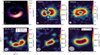Fig. 1

Dust continuum (top left; Yang et al. 2023) and moment-0 maps of the ¹³CO.J=3−2 (top centre; Leemker et al. 2023) and .J=6−5 (top right; van der Marel et al. 2016), and the SO₂ J=6_4,2–6_3,3 (bottom left), CH₃OH J=13₋₁−13₀ (bottom centre), and H₂CO J=5_0,5−4_0,4 (bottom right) transitions. The white star in the centre indicates the approximate location of the host star, whereas the resolving beam is indicated in the lower left. The red circle and cross provide, respectively, the peak flux position of the SO₂ and CH₃OH transitions in the bottom left and centre plots, whereas the red square denotes the peak flux position of the H₂CO transition in the bottom right plot. In addition, the arrows in the ¹³CO .J=3−2 transition indicate where the emission is affected by the cloud absorption.

3 Methods

3.1 Identifying detected transitions

The various SO₂, CH₃OH, and H₂CO transitions are, for each separate pixel, identified using the ‘Leiden Atomic and Molecular Database’ (LAMDA; Müller et al. 2001; Schöier et al. 2005; Wiesenfeld & Faure 2013; Rabli & Flower 2010; Balança et al. 2016). We limit our search to transitions with Einstein-A coefficients of A_ul ≥ 10⁻⁶ s⁻¹ and upper level energies of E_up ≤ 500 K, as lines with lower Einstein-A coefficients and higher upper level energies are not detected. For each pixel and spectral window, we obtain the corresponding spectrum in units of Jy beam⁻¹. The spectra extracted for the pixel where the moment-0 maps peak (highlighted in Figure 1) are shown in Figures B.1, B.2, and B.3 for SO₂, CH₃OH, and H₂CO, respectively. Within each spectrum, we consider all transitions with peak fluxes above three times the root mean square (RMS) as detections. As we retrieve spectra for each pixel and all spectral windows, we determine the RMS in each spectrum using an automated approach consisting of various steps: first, the residual variation in the continuum-subtracted baseline is determined using an iterative, 2σ-outlier masking process and a Savitzky-Golay filter (Savitzky & Golay 1964). The Savitzky-Golay filter allows one to smooth the data using a low-order polynomial over a subset of the data, without altering the underlying shape of the spectrum. We filtered the data using third-order polynomials that smoothed the data every 100 data points. Secondly, the standard deviation (SD) of the residuals, after subtracting the final Savitzky-Golay filter from the 2σ-outlier masked spectrum, is obtained. Finally, we identify and mask all emission lines from the full spectrum, by removing all emission lines that have fluxes above 3× the aforementioned SD. The RMS is, subsequently, obtained from the resulting line-free spectrum. Overall, we find RMS values of ~1 mJy beam⁻¹ for the Cycle 8 observations, very similar to the values listed in Table 6 of Booth et al. (2024). The RMS varies between ~ 1.0–1.5 mJy beam⁻¹ for the Cycle 5 observations, in agreement with the value listed in van der Marel et al. (2021) of ~1.2 mJy beam⁻¹.

From our list of detected transitions, we have removed transitions which are blended with other transitions of the same molecule with different excitation conditions and/or blended with transitions of other molecules. However, we have kept the transitions that are blended with the transitions of the same molecule that have the same Einstein-A coefficient and upper level energy. This allowed us to include two pairs of CH₃OH transitions. As both transitions have the same excitation conditions and, therefore, are expected to contribute equally to the observed line, we assume that half of the observed line flux can be attributed to each of the transitions. Furthermore, through trial and error and visual inspection of the image cubes and line profiles, we have removed additional SO₂ transitions for which we could not confidently distinguish between emission and 3σ noise spikes, i.e. features that appear only locally and do not follow the emission morphologies (i.e. do not follow the same pattern, such as Keplerian rotation, or display different line profiles) seen for stronger transitions. All detected transitions are listed in Table A.1, whereas the blended transitions or those dominated by noise are listed in Table A.2.

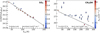Fig. 2

Rotational diagrams for SO₂ (left) and CH₃OH (right) at the peak flux positions of their 6_4,2−6_3,3 and 13₋₁−13₀ transitions, respectively. The colour bar indicates the value for A_ul (×10⁻⁴) of the transitions.

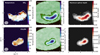Fig. 3

Temperature (left column), column density (middle column), and maximum optical depth (right column) maps for SO₂ (top) and CH₃OH (bottom).

3.2 Integrated intensity and rotational diagram analysis

We infer the excitation conditions (rotational temperature and column density) using a rotational diagram analysis. We obtain integrated fluxes by fitting Gaussian line profiles. As the flux from individual pixels is not independent, we consider the beam area to be the emitting area in our calculations. In addition, we follow the method described by, for example, Banzatti et al. (2012) to create model intensities, which, subsequently, are fitted to inferred values. In the calculation of the optical depth, we have used a line width of $Δ V_{line} = \sqrt{Δ V_{thermal}^{2} + Δ V_{turbulence}^{2}} = 0.2 km s^{- 1}$ $\Delta {V_{{\rm{line}}}} = \sqrt {\Delta V_{{\rm{thermal}}}^2 + \Delta V_{{\rm{turbulence}}}^2} = 0.2{\rm{km}}{{\rm{s}}^{ - 1}}$ . This line width is a combination of the thermal line width (expected to be of the order of ~0.15 km s⁻¹) and the intrinsic width due to local turbulence, which can also reach values of ~0.1 km s⁻¹ (see, e.g. Paneque-Carrefio et al. 2024). Additionally, we have calculated 3σ upper limits, following the description of Carney et al. (2019), for the pixels for which we have not created a rotational diagram.

4 Results

Below we present the rotational diagrams (Figure 2) for SO₂ and CH₃OH. In addition, we show the resulting temperature, column density, and optical depth maps (Figures 3 and 4 and line profiles (Figures B.1, B.2, and B.3) retrieved for the molecules at the peak position of their J=64,2-63,3, J=13₋₁−13₀, and J=5_0,5−4_0,4 transitions, respectively. These peak positions are highlighted in Figure 1. Our analysis assumes that the molecular emission is optically thin, for a discussion on the potential effects of optically thick emission, see Section 5.3.

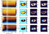Fig. 4

Line ratios for the different pairs of H₂CO transitions. The left panels show the RADEX calculations, with the colour map indicating the various ratios. The white contours indicate the values of 0.3, 0.5, and 0.7, whereas the red contour indicates the disk integrated ratio from van der Marel et al. (2021). The panels in the second column indicate the ratios derived for the pixels where both transitions are detected, using the colour scheme as for the left panels. The final two columns display the derived temperatures for gas densities of $n_{H_{2}} = 10^{7} {cm}^{- 3}$ ${n_{{{\rm{H}}_2}}} = {10^7}{\rm{c}}{{\rm{m}}^{ - 3}}$ (representative of the disk’s atmosphere, z/r ≳0.2) and 10⁸ cm⁻³ (representative of the disk’s midplane). The white solid, dashed, and dotted contours indicate temperatures of 200 K, 300 K, and 400 K, respectively.

4.1 SO₂

At the peak position of the integrated intensity map of the J=6_4,2≳6_3,3 transitions of SO₂, we detect 13 isolated transitions (see also Table A.1). The rotational diagram for this position is displayed in the left panel of Figure 2, while the line profiles are shown in Figure B.1. The left-side of Figure D.1 displays the intensity ratios between the observations and the modelled intensities. We find a well-constrained rotational diagram and derive a rotational temperature of T=54.8±1.4 K and a peak total column density of N=(4.8±0.1)×10¹³ cm⁻². The upper limits on the column density, for pixels with an insufficient number of detected transitions, range between ~2.0×10¹³ and ~2.4× 10¹³ cm⁻², which are a factor of ~2 lower than found at the peak position. We also find, for all pixel positions, a maximum optical depth of τ ~ 0.1, suggesting that the SO₂ emission is optically thin. The optical depth is further discussed in Section 5.3. The final maps (temperature, column density, and optical depth) are displayed in the left panel of Figure 3. Given the low inferred uncertainties on the temperatures (of the order of a few Kelvin, see Figure D.2), the hotter temperature (~70 K) at the inner edge is significantly higher than that at the outer edge (~40 K). The higher temperatures inferred at some of the edge pixels are likely due to fewer transitions detected and weaker line fluxes, and are, therefore, more uncertain (see also Figure D.2).

The well-behaved rotational diagram of SO₂ points towards thermalised emission. As the gas densities necessary for the SO₂ emission to become thermalised are only found in a layer just above the midplane, we suggest that the emission must originate from this layer deep inside the disk (see also Section 5.2.2), which is also consistent with the derived rotational temperature.

4.2 CH₃OH

For CH₃OH, we observe 22 transitions at the peak position of the integrated intensity map of the J=13₋₁ −13₀ transition that are either unblended or blended with other CH₃OH lines with similar parameters (see also Table A.1). The rotational diagram and the ratios between the observations and modelled intensities are shown in the right panels of Figures 2 and D.1, the line profiles are displayed in Figure B.2, and the final maps are shown in the lower row of Figure 3. Using these transitions, we derive a rotational temperature of $T = {125.5}_{- 3.5}^{+ 3.7}$ $T = 125.5_{ - 3.5}^{ + 3.7}$ K and a total column density of N=(1.2±0.1)×10¹⁴ cm⁻² at the peak position. The upper limits on the column density are of the order of ~5.8×10¹³ cm⁻² to ~6.9×10¹³ cm⁻², a factor of ~2 lower than the peak value. We find a maximum optical depth of T ~ 0.03, suggesting that the CH₃OH emission is optically thin. In contrast with that of SO₂, the rotational diagram of CH₃OH shows a large scatter between the data points, this is further discussed in Section 5.1.

4.3 H₂CO

The pixel-by-pixel rotational diagram analysis for the 7 observed H₂CO transitions in Cycle 5 (van der Marel et al. 2021) proved to be more difficult and we were not able to retrieve reliable values for the rotational temperature and column density, likely due to a combination of the optical depth (discussed later in this section), a mixture of the ortho- and para-transitions, and sub-thermal excitation (see Section 5.1). In order to obtain a pixel-by-pixel temperature map, we derived the temperatures using various line ratios. Similar to van der Marel et al. (2021), we use RADEX to obtain line ratios for various values of the kinetic temperature (T_kin in K) and the gas density ( $n_{H_{2}}$ ${n_{{{\rm{H}}_2}}}$ in cm⁻³). Following van der Marel et al. (2021) we used a column density of $n_{H_{2} CO = 10^{14} {cm}^{- 2}}$ ${n_{{{\rm{H}}_2}{\rm{CO}} = {{10}^{14}}{\rm{c}}{{\rm{m}}^{ - 2}}}}$ in the calculations, at which the emission should be optically thin. Additionally, we have used the default line width of 1 km s⁻¹ within the RADEX calculations. More details on the calculations can be found in Section 5.1. We determine the temperature, using a simple minimisation of the ratios obtained through RADEX with the inferred ratios from the observations, for gas densities of $n_{H_{2}} = 10^{7}$ ${n_{{{\rm{H}}_2}}} = {10^7}$ cm⁻³ and 10⁸ cm⁻³, which, respectively, correspond to the disk’s atmosphere and the midplane.

We have determined the line ratios for one pair of orthotransitions (5₃₃−4₃₂ /5₁₅−4₁₄) and three pairs of para-transitions (52,4−4_2,3/5_0,5−40,4, 5_4,2−4_4,1/5_0,5−4_0,4, and 5_4,2−4_4,1/5_2,4−4_2,3). The second and third pairs of the para-transitions allow us to investigate how the ratios change for transitions with different upper level energies, as the line excitation and, therefore, the observed flux and ratios are temperature sensitive. The ratios and inferred temperature maps are displayed in Figure 4. We highlight our findings for each line pair separately in Appendix C.

Overall, we can infer from the ratios that the temperatures of H₂CO across the dust trap can be expected to be of the order of T ~ 150−350 K, with the highest temperatures found in the centre of the dust trap. As discussed above, this is generally similar to, albeit slightly higher than, the ratios derived from the disk-integrated values of van der Marel et al. (2021). Such high temperatures are not unexpected given the high upper level energies of some of the H₂CO transitions detected in the disk of IRS 48 (i.e. the J=5_4,2−5_4,1 and J=5_4,1 −5_4,0 transitions with E_up=240.7 K or the warm transition of J=9_1,8−8_1,7 with E_up=174 K detected in van der Marel et al. 2014). Compared to the other molecules, SO₂ and CH₃OH, we find that the temperatures are significantly higher than those of SO₂, but are similar to and/or higher than those of CH₃OH. These high temperatures indicate that the emission must come from high up in the disk, as suggested before by van der Marel et al. (2021). Therefore, the temperatures derived assuming a gas density of $n_{H_{2}} = 10^{7}$ ${n_{{{\rm{H}}_2}}} = {10^7}$ cm⁻³ should provide the best constraints. These are, however, also more limited by the ratios and the involved temperature sensitivity of the transitions. For the remainder of this work, we assume that the temperature derived for H₂CO is at least -150 K.

For a temperature of T=150 K, a column density of N =10¹⁵ cm⁻², and a gas density of $n_{H_{2}} = 10^{7}$ ${n_{{{\rm{H}}_2}}} = {10^7}$ cm⁻³, the RADEX calculations yield a maximum optical depth of τ ~ 1.9, suggesting that some of the transitions may be (moderately) optically thick in the outer edges of the dust trap (i.e. the regions where probe temperatures of T_rot ~ 150 K, see Figure 4). For the same conditions, but a temperature of T= 350 K, we infer a maximum optical depth of τ ~ 0.6, suggesting that the emission in the central regions are more optically thin.

5 Discussion

In the following sections, we discuss our results. We start by discussing the well-behaved rotational diagram of SO₂, which is in contrast with that for CH₃OH which is dominated by large scatter. This points towards SO₂ being thermally excited, while CH₃OH is sub-thermally excited (Section 5.1). In Section 5.2, we discuss the temperature and resulting vertical structures of the disk, whereas the optical depth and radial structure are discussed in Section 5.3. Finally, we highlight potential follow-up observations in Section 5.4, which are needed to fully resolve the molecular emission and to infer more information on the column densities.

5.1 Sub-thermal excitation

Given the well-behaved rotational diagram of SO₂, characterised by very limited scatter, we expect the emission to be (close to) thermalised. In stark contrast with this, is the large scatter observed in the rotational diagram of CH₃OH, which is likely due to the effects of sub-thermal excitation. As shown in Figure 6 of Johnstone et al. (2003), higher energy lines of CH₃OH have higher critical densities and are, subsequently, not thermalised at relatively low densities (i.e. n=10⁷ cm⁻³). A rotational diagram can still yield a single excitation temperature using a rotational diagram, but this value is much lower than the kinetic one, because the levels are not thermalised. By increasing the density (to, for example, n=10⁹ cm⁻³) in their RADEX calculations, Johnstone et al. (2003) found that the lines became thermalised tended towards the physical input conditions. In particular, the derived rotational temperature started to represent the input kinetic temperature.

We have used RADEX (van der Tak et al. 2007) to investigate at what gas densities the SO₂, CH₃OH, and H₂CO emission thermalises. We have run the calculations for each molecular species, including all transitions with frequencies <1000 GHz, but limiting the transitions to those with E_up ≤ 300 K and A_ul ≥ 10⁻⁶ s⁻¹ to cover similar properties as our observed transitions, as only using the detected transitions did not yield sensible results. The number of transitions is too sparse to derive meaningful rotational temperatures for the entire grid. We ran the calculations separately for the A- and E-transitions of CH₃OH and for the ortho- and para-transitions of H₂CO. The calculations are run over grids of T_kin (10 K to 200 K in steps of 10 K) and $\log_{10} (n_{H_{2}})$ ${\log _{10}}\left( {{n_{{{\rm{H}}_2}}}} \right)$ (5 to 12 in steps of 0.1, with $n_{H_{2}}$ ${n_{{{\rm{H}}_2}}}$ in units of cm⁻³). In our calculations, we have kept the column density at a fixed value of N=10¹² cm⁻², which ensures optically thin emission and we used, similarly as in Section 4.3, the default line width of -1 km s⁻¹ . For each calculation, we infer the rotational temperature by fitting a straight line (y = ax + b) through all the retrieved RADEX integrated fluxes, where the rotation temperature is given by the slope, a = −1/T_rot. Figure 5 displays the percentile difference between the input kinetic temperature and the derived rotational temperature (∆T) from the RADEX calculations. For smaller percentages, the lines are thermalised. The contours (solid, dashed, and dashed-dotted) indicate where the differences are, respectively, ∆T=1%, 5%, and 10%. Above these contours (i.e. for higher densities), the difference becomes smaller and the emission is thermalised, whereas below these contours the differences become larger and the lines are not thermalised. Figure 5 also indicates the gas density, up to a height of 20 au, at the location of the 1RS 48 dust trap, following the DALI model of Leemker et al. (2023) (see also Section 5.4), and the derived excitation conditions from the rotational diagrams: T ~ 55 K for SO₂, T ~ 130 K for CH₃OH, and the lower end of the derived temperature range (T ~ 150 K) for H₂CO.

We find that SO₂ thermalises at densities of $n_{H_{2}} ~ 10^{8}$ ${n_{{{\rm{H}}_2}}}\~{10^8}$ cm⁻³ and higher. As the rotational temperature of SO₂ is well-constrained at T ~ 55 K, this requires that the SO₂ emission should be thermalised. However, densities of $n_{H_{2}} ~ 10^{8}$ ${n_{{{\rm{H}}_2}}}\~{10^8}$ cm⁻³ are only achieved near the midplane of the disk at heights of ~ 5 au (z/r < 0.1, see also Section 5.4), suggesting that the SO₂ may originate from deep inside the disk. The emitting height of SO₂ is further discussed in Section 5.2.

For H₂CO we find that the emission thermalises at similar densities as S0₂, however, the derived temperatures are significantly higher, suggesting that the H₂CO emission does not originate from the same layer as SO₂. CH₃OH requires, on the other hand, even higher densities of $n_{H_{2}} > 10^{9} {cm}^{- 3}$ ${n_{{{\rm{H}}_2}}} > {10^9}{\rm{c}}{{\rm{m}}^{ - 3}}$ . Combining these dust trap densities with the derived rotational temperatures, we infer that the emission of both CH₃OH and H₂CO may be sub-thermally excited. Therefore, the presented rotational temperatures are considered to underestimate the kinetic temperature and non-LTE approaches should be used to correctly derive the excitation conditions. As CH₃OH requires higher gas densities to be thermalised compared to H₂CO (i.e. the differences, ∆T, are larger), we expect that the underestimation of the kinetic temperature is larger for CH₃OH than for H₂CO (as indicated in Figure 5). Therefore, we expect that the CH₃OH and H₂CO may actually probe very similar temperatures and, as suggested by van der Marel et al. (2021), that the species may originate from the same high layer inside the disk.

We reiterate that the 1RS 48 disk has exceptionally low gas and dust masses. For disks with higher masses and, therefore, higher densities, the molecular emission is more likely to be thermally excited. Therefore, observations (or surveys) of massive disks, covering multiple (≥3 or at least 2, if the upper level energies are significantly different) transitions of the same molecular species, could be used to infer the (gas) temperature and chemical structure from their molecular line emission. For these less massive disks, a non-LTE analysis is a necessary and powerful tool to infer the excitation conditions.

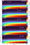Fig. 5

RADEX grids for SO₂ (top panel), A- and E-type CH₃OH (second and third panels), and ortho- and para-H₂CO (bottom two panels) showing the percentile difference between the kinetic and rotational temperature (∆T), as a measure of thermalised transitions. The contours (solid, dashed, and dashed-dotted) in each panel indicates when ∆T=1%, 5%, and 10%, respectively. Above these contours the lines will be thermalised. The white shaded area indicates the gas density of the dust trap according to the DALI model (Leemker et al. 2023). Finally, the arrows indicate the derived excitation temperatures of T ~ 55 K for SO₂ and T ~ 130 K for CH₃OH. For H₂CO we show the rotational temperature of 150 K, the lower value of the inferred temperature range.

5.2 Temperature and vertical structure

In the following section, we discuss the resulting temperature (Section 5.2.1) and vertical structure (Section 5.2.2) of the disk, as interpreted from our results.

5.2.1 Temperature structure

Using our temperature maps (top row in Figure 3), we assess how the temperature may vary across the 1RS 48 dust trap. In Figure D.2, we display the derived lower and upper uncertainties for the temperature maps of SO₂ and CH₃OH. The uncertainties are found to be the highest for pixels near the edge, for which often also the highest temperatures are found. This is very likely due to the fact that fewer transitions are detected and the line emission is not as strong as for pixels closer to the centre (see also Figure F.l). The temperature map for CH₃OH does not show a clear temperature structure but is rather constant across the entire disk with temperatures of T ≳ 125 K. The SO₂ map, on the other hand, shows hints of a potential radial temperature gradient, which is generally expected to be present in disks. The temperature closer to the host star is hotter (T ~ 70 K) compared to the temperature at the outer edge (T ~ 40 K).

Overall, we find that the uncertainties for SO₂ and CH₃OH are nearly uniform (σ_T ≲ 5 K) across the molecular emission extent. Additionally, Figure D.3 show the uncertainties for the column density maps. We find that the uncertainties on the column density are uniform across the maps of all three molecular species, of the order of <10%. As our temperature uncertainties are of the order of σ_T ≲ 5 K, we expect this radial temperature gradient in the SO₂ map to be real. The observed radial decrease in the temperature is of the order of 10 K to 30 K when considering the uncertainties. The DALI model suggests, on the other hand, that the temperature for the expected emitting layer of SO₂ (see Section 5.2.2), remains fairly constant between 40 and 70 K.

As the asymmetric dust trap of 1RS 48 may be the result of a vortex present in the disk, this vortex could also influence the observable temperature structure. As discussed by Lovelace & Romanova (2014), if the vortex is the result of the RWI, the vortex must be anticyclonic (i.e. rotate clockwise) for it to generate a pressure maximum that can trap the dust. Most of the recent work on vortices has gone into their existence, evolution, and stability (e.g. Lovelace et al. 1999; Meheut et al. 2012b,a, 2013; Lovelace & Hohlfeld 2013), or into their relationship with forming planets (e.g. Hammer et al. 2017, 2019, 2021; Hammer & Lin 2023). Little work (see, for example, Huang et al. 2018; Leemker et al. 2023) has focused on how the gas and chemistry may be affected by the vortices. Vortices perturb the motion of the gas, so intuitively, such a perturbation may also be visible in the temperature structure. If the gas perturbation follows the anticyclonic rotation of the vortex, gas with slightly higher temperature would be rotating away from the host star, whereas cooler gas would move towards the host star. This is also visualised in Figure 6. The strength of this effect would depend on the rotational timescale of the vortex, which itself is set by the vorticity (Meheut et al. 2013): the faster the vortex rotates, the stronger the effect will be. As vortices predominantly arise in the midplane, their effect on the dust and gas should be most notable for molecular emission originating from close to the midplane, but may be negligible in elevated layers, where UV heating dominates. As we expect SO₂ to emit from close to the midplane and we do not see an azimuthal variation that could be induced by a potential vortex, the temperature variation induced by such a vortex can only be of the order of ~2 K, given the small uncertainties. CH₃OH is, on the other hand, together with H₂CO expected to emit from an elevated layer ~10-15 au (z/r ~ 0.17-0.25) above the midplane (van der Marel et al. 2021). Therefore, we expect not to see any variation in the temperature related to a potential vortex. Only if vertical mixing, which is expected to play a role in liberating the molecular species from the icy dust mantles in the IRS 48 disk, can transmit the effect from a vortex to elevated regions, a different temperature structure may be found in the molecular emitting layers. Detailed models that constrain the vorticity and include vertical mixing can be used to investigate the interplay between the dust and gas in vortices and, subsequently, are necessary to investigate the potential influences of vortices on the temperature structures of disks.

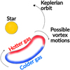Fig. 6

Cartoon visualising the expected effect of the vortex on the temperature structure. Hotter gas, due to UV heating, will be counteracted by colder gas being brought in due to the potential vortex motions, which primarily acts in the midplane. This effect is not observed in the IRS 48 disk, unless the temperatures variations are very small.

5.2.2 Vertical structure

In addition to the temperature maps, we have measured the temperature using the brightness temperature (T_b) of optically thick emission, i.e. from the dust continuum or from one of the CO isotopologues. Using Planck’s law, we have calculated the brightness temperature of the high-resolution, optically thick 0.9 mm continuum emission (Yang et al. 2023) and of the ¹³CO J=3−2 (Leemker et al. 2023) and J=6−5 (van der Marel et al. 2016) transitions. The brightness temperature maps are displayed in Figure 7. We find a peak brightness temperature of T_b ~ 32 K for the dust continuum, which is only slightly higher (∆T_b ~ 5 K) than that found in van der Marel et al. (2021), likely due to the difference in the beam sizes. The higher brightness temperature determined here confirms the notion that the temperature of the dust in the disk’s midplane is too high for CO freeze-out and in situ COM formation through the hydrogenation of CO (Watanabe & Kouchi 2002; Fuchs et al. 2009; Santos et al. 2022). However, CO may still react with solid-state OH to form CO₂, even though the temperatures are above its sublimation temperature (Terwisscha van Scheltinga et al. 2022).

As the CO emission is affected by foreground cloud absorption (Bruderer et al. 2014), the temperature can only be estimated for select emission channels. We find peak brightness temperatures of T_b,3-2 ~ 110 K and T_b,6-5 ~ 135 K, from the absorption-free channels of the optically thick ¹³CO J=3−2 and J=6−5 transitions, respectively. Based on these derived temperatures, and those derived for SO₂, CH₃OH and H₂CO, we can infer the vertical emission structure of the disk. We expect CH₃OH and H₂CO to trace the highest temperatures, given their derived temperatures and the notion that the emission is sub-thermally excited, and, therefore, they should arise from a higher emitting layer. The ¹³CO, probing a slightly colder temperature, should originate from a slightly deeper layer in the disk, under the assumption that the emission is fully resolved (Leemker et al. 2022), while the SO₂ should originate from the deepest vertical layer. The notion that SO₂ originates from deep inside the disk, based on the temperature, is supported by our RADEX calculations (see Section 5.1), which show that SO₂ becomes thermalised at densities of n_gas ~ 10⁸ cm⁻³. These densities are only reached in the layers close to the midplane, with heights of ≲5 au (or z/r<0.1, see also Section 5.4). Therefore, under the assumption of thermalised emission, the SO₂ emission must originate from this layer just above the midplane. We also consider the radial locations of the emission to support our vertical structure posed above. We note that the SO₂ emission peaks at larger distances, by ~10 au, than both CH₃OH and H₂CO (see Booth et al. 2024).

5.3 Optical depth and emission structure

Below, we discuss the optical depth of the various molecules (Section 5.3.1). In addition, we also discuss the required radial extent of the emission to become optically thick.

5.3.1 Optical depth

For the chosen turbulent line width (∆V_line=0.2 km s⁻¹ ) our analysis points towards potentially optically thin emission. However, it is still possible that the molecular emission, in particular that of H₂CO, is optically thick. Considering a previously derived iso-topologue ratio, H₂CO/H₂¹³CO~4 (Booth et al. 2024), it is very likely that its emission is optically thick. As the spatial resolution of the used observations is low, one likely explanation for our analysis pointing towards optically thin emission is that the actual emitting areas are smaller than currently can be probed. As can be seen in Figure 1, the radial extent is of a similar size as that of the beam. The azimuthal extent of both SO₂ and H₂CO is, on the other hand, larger than a single beam. Therefore, we conclude that the azimuthal extent is resolved, whereas the radial one is not.

To test for what emitting areas, parameterised by the beam radius (assuming a circular beam), and values for the local (turbulent) line widths we can ensure optically thick emission, we have explored grids over both parameters. We have run the grids for the same transitions as used throughout our analysis: SO₂ J=6_4,2−6_3,3, CH₃OH J=13₋₁4−13₀, and H₂CO 7 =5_1,5−4_1,4. For H₂CO, we have used a higher resolution (both spatial and spectral) transition that has been presented in Booth et al. (2024) (see also Figure E.1), which is of the same spectral and spatial resolution as the SO₂ and CH₃OH transitions. In our calculations of the optical depth, we have used fixed rotational temperatures of T_rot=55 K for SO₂, T_rot=150 K for CH₃OH, and T_rot=150 K and T_rot=350 K for H₂CO to represent the range of temperatures found. Our grid of the line width extends up to 1.0 km s⁻¹. If the line profiles are only thermally broadened, they will be of the order of ~0.15 km s⁻¹, but local turbulence can additionally broaden the lines by ~0.1 km s⁻¹ (see, e.g. Flaherty et al. 2020, 2024; Paneque-Carreño et al. 2024).

The inferred optical depths for our grids of turbulent line widths and beam radii are displayed in Figure 8. As can be seen, we require beam radii of ≲ 8 au for the H₂CO emission to become optically thick at a temperature of T_rot ~ 350 K. For the lower temperature of T_rot ~ 150 K, a larger beam area of ≲ 16 au is sufficient for optically thick emission. These lower temperatures should hold for the outer edges of the dust trap, whereas the warmer temperature accounts for the central region (see also Section 4.3). The SO₂ emission also becomes optically thick for an emitting radius of ≲8 au, whereas the CH₃OH emission requires slightly smaller radii. For smaller line widths (∆V_line < 0.2 km s⁻¹), we find that the emission becomes optically thick for larger beam areas.

We, thus, propose a scenario in which the emission (in particular that of H₂CO) originates from a small radial ‘sliver’ with an approximate width of ≲10 au. This ‘sliver’ must be located at the inner edge of the dust trap for CH₃OH and H₂CO to conform with the current hypothesis that the observed molecules are in the gas phase following thermal sublimation (see, e.g., van der Marel et al. 2021; Booth et al. 2021, 2024). While SO₂ emission is known to originate from a larger radial distance (Booth et al. 2024), it is still possible that the emission originates from a similar ‘sliver’, only placed at a larger radial distance, coming from close to the midplane, and is located closer to the outer edge of the dust trap.

For comparison, we have estimated, from the high-resolution dust observations (Yang et al. 2023), that the dust trap has a width of -26.5 au (see also Figure 8). Interestingly, from imaging of the H₂CO J=5_1,5−4_1,4 transition with superuniform weighting (see right panel of Figure E.1), a smaller width of the emission is inferred. We note that the radial extent is still unresolved with this weighting scheme. The resulting beam (0.22″ × 0.18″) has a width of ~25 au, which is bigger than the proposed width of the ‘sliver’. Finally, we note that one of the models presented by van der Marel et al. (2021) also suggests this sliver theory for the H₂CO theory. In particular, their full model, where the large grain population is increased throughout the entire dust column instead of settled to the midplane, with a surface density of Σ_d=5.0 g cm⁻² at 60 au, has the H₂CO distributed over the entire vertical extent, but radially only between 60 and 70 au (see their Figure C.2). We have visualised our proposed emission scheme in Figure 9, based on the temperatures as discussed in Section 5.2 and the potential radial extent of the molecules as discussed here.

The discussion above suggests that the emitting areas of the molecules are radially unresolved and, subsequently, the emission is beam diluted. This has previously already been discussed in Brunken et al.(2022) and Booth et al. (2024). Beam dilution results in an underestimation of the inferred column densities. Higher-resolution observations with spatial resolutions of <0.1″ (translating to a resolution of < 13.5 au for the distance of IRS 48) are needed to obtain better constraints on the column densities. Using the following equation, ${DF}^{- 1} = \frac{Ω_{source}^{2}}{Ω_{beam}^{2} {+Ω}_{source}^{2}},$ ${\rm{D}}{{\rm{F}}^{{\rm{ - 1}}}}{\rm{ = }}{{{\rm{\Omega }}_{{\rm{source}}}^{\rm{2}}} \over {{\rm{\Omega }}_{{\rm{beam}}}^{\rm{2}}{\rm{ + \Omega }}_{{\rm{source}}}^{\rm{2}}}},$

we provide an estimate on the dilution factor for the molecular emission, assuming the emission comes from a circular region with a total width of 10 au, as proposed above with our ‘sliver’ theory. As determined by the column densities on a pixel-by-pixel basis, we take the $Ω_{beam}^{2}$ $\Omega _{{\rm{beam}}}^2$ to be equal to the beam size of the current observations, whereas we set $Ω_{source}^{2}$ $\Omega _{{\rm{source}}}^2$ equal to the area of the circular region. This yields DF⁻¹ ~ 0.002 or, in other words, an underestimation of the column density by a factor of ~ 500.

For our derived column densities (see Section 4) and given the uncertain optical depths, we derive lower limits on the fractional abundances, with respect to H₂ (Σ_𝑔=0.25 g cm⁻² or $N_{H_{2}} ~ 7 \times 10^{22}$ ${N_{{{\rm{H}}_2}}}\~7 \times {10^{22}}$ cm⁻³; van der Marel et al. 2016; Leemker et al. 2023), of $N_{{SO}_{2}} / N_{H_{2}} ~ 7 \times 10^{- 10} - 3 \times 10^{- 9}$ ${N_{{\rm{S}}{{\rm{O}}_2}}}/{N_{{{\rm{H}}_2}}}\~7 \times {10^{ - 10}} - 3 \times {10^{ - 9}}$ and $N_{{CH}_{3} OH} / N_{H_{2}} ~ (1 - 8) \times 10^{- 9}$ ${N_{{\rm{C}}{{\rm{H}}_3}{\rm{OH}}}}/{N_{{{\rm{H}}_2}}}\~\left( {1 - 8} \right) \times {10^{ - 9}}$ . Assuming that we underestimate the column densities by a factor of ~500, these fractional abundances become $N_{{SO}_{2}} / N_{H_{2}} ~ 3 \times 10^{- 7} - 2 \times 10^{- 6}$ ${N_{{\rm{S}}{{\rm{O}}_{\rm{2}}}}}/{N_{{{\rm{H}}_2}}}\~3 \times {10^{ - 7}} - 2 \times {10^{ - 6}}$ and $N_{{CH}_{3} OH} / N_{H_{2}} ~ 7 \times 10^{- 7} - 4 \times 10^{- 6}$ ${N_{{\rm{C}}{{\rm{H}}_3}{\rm{OH}}}}/{N_{{{\rm{H}}_{\rm{2}}}}}\~7 \times {10^{ - 7}} - 4 \times {10^{ - 6}}$ . Compared to two other Herbig stars, HD 100546 and HD 169142, we find that our derived column densities for CH₃OH are of the same order of magnitude (Booth et al. 2023 and Evans et al. in prep.). However, we note that our column densities may be underestimated by this factor of -500.

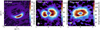Fig. 7

Brightness temperature maps of the dust continuum (left) and the ¹³CO .J=3−2 (middle panel) and ¹³CO .J=6−5 (right panel) transitions. The yellow stars in the centre indicate the approximate location of the host star, while the resolving beams are indicated by the white ellipses.

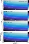Fig. 8

Optical depth (given in log₁₀-space) grids for a range of beam radii (assuming circular beams) and turbulent line widths (∆V) for SO₂ J=6_4,2−6_3,3 (at T_rot=55 K), CH₃OH 7=13₋₁−13₀ (at T_rot=150 K, accounting for the underestimation of the temperature due to sub-thermal excitation), and H₂CO J=5_1,5−4_1,4 (at T_rot=150 K and T_rot=350 K). The contour lines indicate values of τ=1, 10, and 100. The dotted black line indicates the radial FWHM of the dust trap (FWHM_dust ≃ 26.5 au), found using the high-resolution observations of Yang et al. (2023). The vertical dashed line indicates a turbulent line width of ∆V_line=0.2 km s⁻¹, the lower value used in our analysis.

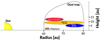Fig. 9

Cartoon visualising our proposed radial vertical emission scheme, containing SO₂ (blue), ¹³CO (orange), and H₂CO and CH₃OH (red). The radial and vertical emission locations are based on the derived temperatures, the proposed sliver theory, and the assumption that the ¹³CO emission is spatially resolved.

5.3.2 Continuum affecting the line emission

One additional concern for our derived excitation properties is the potential effect of the dust continuum on the observed molecular emission, in particular, that of CH₃OH and H₂CO. The continuum emission can impact the line emission in two ways (Boehler et al. 2017; Weaver et al. 2018; Isella et al. 2018; Rab et al. 2020; Bosman et al. 2021; Rosotti et al. 2021; Nazari et al. 2023): (1) if the lines themselves are optically thick, the continuum subtraction procedure may overestimate the contribution of the continuum at the line centre. The subtraction would, subsequently, result in an oversubtraction of the continuum. This effect maximises once the continuum also becomes optically thick. (2) On the other hand, if the line is optically thin and the continuum is optically thick, up to half of the total emission, originating from the backside of the disk, may be blocked by the continuum.

As it is expected that the H₂CO emission is optically thick and polarisation observations of the IRS 48 continuum and accompanying modelling works by Ohashi et al. (2020) suggest that the dust continuum at 0.86 mm (~348.6 GHz) is optically thick (τ_dust ~ 7.3), it is not immediately clear which effect is at play. Nonetheless, the channel maps of the CH₃OH J=13₋₁−13₀ and H₂CO J=5_1,5−4_1,4 transitions show that the observed emission is affected by the continuum, see Figures G.1, G.2, and G.3. The channel maps for CH₃OH and H₂CO show a decrease, most notable in the 4.8-6.6 km s⁻¹ velocity range for CH₃OH and 3.9– 7.5 km s⁻¹ range for H₂CO, in the line emission near the peak location of the dust continuum, which is not visible in those of the SO₂ J=6_4,2−6_3,3 transition. Therefore, we expect that we are not probing the full line flux of these molecules, either due to continuum oversubtraction or the continuum blocking emission originating from the backside of the disk. Given that the effect is most notable in the channel maps of CH₃OH and H₂CO, and not in those of SO₂, we propose that continuum oversubtraction is the likely effect. Especially considering that the SO₂ originates from near the midplane, where the secondary effect (dust blocking the emission) could be even stronger than for the elevated layers, i.e. more than half of the emission could be blocked. This suggests that CH₃OH, in addition to H₂CO, should be optically thick. Therefore, we propose that the ‘sliver’ theory mentioned above should also hold for CH₃OH. This, in addition to the beam dilution, results in an underestimation of the column density by as much as a factor of 500.

5.4 Future observations

Any conclusions on the chemistry are currently limited by the spatial and spectral resolution of the observations. Therefore, to be able to infer more information on the chemistry (i.e. column densities), we need higher resolution (both spatially and spectrally) observations that are able to test our ‘sliver’ theory proposed in Section 5.3 for H₂CO and potentially CH₃OH. At the distance of IRS 48 (d ~ 135 pc), an angular resolution of ~0.1″ is needed to retrieve the necessary beam radius of ~8 au. In addition, these observations may provide more insights into the varying temperature structure, potentially related to the influence of a vortex.

Furthermore, a spectral resolution of ~0.1 km s⁻¹ will ensure resolved line profiles for line widths of ≳0.5 km s⁻¹. This spectral resolution will allow one to infer the vertical emission heights from the channel maps, as recently has been done for a multitude of other inclined disks (Law et al. 2021; Paneque-Carreño et al. 2023; Law et al. 2023b,a, 2024; Urbina et al. 2024). A vertical decomposition of the emission layers could also confirm our notion that the CH₃OH and the H₂CO must come from higher emitting layers compared to ¹³CO, while the SO₂ must originate from deep inside the disk. Additionally, the proposed resolutions will be sufficient to study kinematical signatures that deviate from Keplerian emission at the location of the dust trap, as was performed for the asymmetric HD 142527 disk using CO isotopologues (Boehler et al. 2021).

Finally, as seen in Figure 4, many of the line ratios are limited by the temperature sensitivity of the transitions. In order to better constrain the temperature through these ratios, transitions with higher upper level energies need to be observed. These lines, in addition to the higher-resolution observations, will ensure proper constraints on the temperature, not influenced by effects such as beam dilution.

Fig. 10

Zoom-in of the model structure of the dust trap region of the IRS 48 disk of the gas density (n_gas in cm⁻³, left panel) and gas and dust temperature (both in Kelvin, left and right panels, respectively). The vertical bars indicate the location of the dust trap, extending from 60 to 80 au, while the white contours in the left most panel indicate gas densities between 10⁷ and 10⁸ cm⁻³. The images have been adapted from Leemker et al. (2023).

6 Timescales: Vertical mixing, desorption, and photodissociation

6.1 Methodology

To further determine what sets the observable molecular abundance in the IRS 48 disk, we have calculated multiple timescales at the location of the dust trap: the vertical turbulence mixing timescale, the desorption and freeze-out timescales of SO₂, CH₃OH, and H₂CO, and their photodissociation timescales. Interestingly, the disk of IRS 48 has very low gas and dust masses, with a gas mass of the order of M_gas ~ 1.4×10⁻⁴ M_⊙ (Bruderer et al. 2014), obtained through modelling the observed C¹⁷O J=6–5 flux and found to be consistent with the mass derived from the C¹⁸O observations (van der Marel et al. 2016), and a dust mass of M_dust ~ (6.2±0.6)×10⁻⁵ M_⊙ (Temmink et al. 2023). These masses are lower compared to other Herbig stars, which have disk masses of the order of ~10⁻² M_⊙ (e.g. Stapper et al. 2024). Therefore, the gas densities in the IRS 48 dust trap, even near the midplane, are only of the order of 10⁸ cm⁻³ and drop to 10⁶ cm⁻³ in the surface layers. We have used the inferred properties (i.e. n_gas, T_gas, and T_dust) of the IRS 48 disk as modelled by Leemker et al. (2023) using the thermochemical code DALI (Bruderer et al. 2012; Bruderer 2013). This DALI model is built upon an existing model from Bruderer et al. (2014), van der Marel et al. (2016), and van der Marel et al. (2021), and is described by a radial surface density profile that uses the selfsimilar solution for a viscously evolving disk (Lynden-Bell & Pringle 1974; Hartmann et al. 1998). It consists of deep dust and gas cavities between 1 and 60 au, while the dust trap is placed at 60–80 au. The model is separated into two different models: one representing the dust-trap side (where the dust density distribution has been altered under the assumption that the small grains have grown to larger sizes) and one tailored to the other side of the disk. This model is able to reproduce the continuum emission (at 0.44 mm and 0.89 mm) and the emission of various CO isotopologues. The gas temperature is also well constrained within the model, as it is able to reproduce emission of the CO J=6–5 transition. We refer the reader to Leemker et al. (2023) for all details on the model (see their Appendix B). Figure 10 displays the gas density (in cm⁻³) and the gas and dust temperature of the DALI model in the region of the dust trap. Below, we discuss how the timescales are calculated, whereas their implications on the emission are further discussed in Section 6.2.

We determine the turbulent vertical mixing timescale following the description provided by Xie et al. (1995) and Semenov et al. (2006), where the vertical mixing is set by the turbulent diffusion. The mixing timescale can be approximated as t_mix ~ H² /D_turb, where H is the scale height (taken as H = c_s/Ω_K) and $D_{turb} = α c_{s}^{2} / Ω_{K}$ ${D_{{\rm{turb}}}} = \alpha c_{\rm{s}}^2/{{\rm{\Omega }}_{\rm{K}}}$ is the turbulent diffusion coefficient (in cm⁻² s⁻¹). Here, c_s and Ω_K denote the sound speed (taken to be isothermal) and the Keplerian angular frequency, respectively, while α parametrises the viscosity strength. We have determined the vertical mixing timescales for three commonly used values of α: 10⁻⁴, 10⁻³, 10⁻². For comparison, Yang et al. (2024) find turbulent α parameters, using the scale height ratio prescription of Youdin & Lithwick (2007) and assuming a grain size of 140 µm and a dust surface density of Σ_d=1 g cm⁻², ranging from 10⁻⁴ to 5×10⁻³ for gas-to-dust mass ratios of 3–100 in the IRS 48 disk. As the gas-to-dust mass ratio is expected to be much lower in the dust trap ~0.009–0.04 (Ohashi et al. 2020; van der Marel et al. 2016; Leemker et al. 2023), the α parameter could be even higher. Therefore, our range of α values encapsulates the expected range well. We note that a higher α parameter, for example α=0.1, only changes our results by a factor of 10, i.e. the turbulent diffusion coefficient would increase by this factor, whereas the mixing timescale would decrease by this factor.

The desorption (k_d) and freeze-out (k_f) rates (in s⁻¹) are determined for each molecular species i following the equations given in Tielens & Allamandola (1987) (see also Walsh et al. 2010 and Leemker et al. 2021): $\begin{array}{l} k_{d,i} = v_{0} (i) \exp (- \frac{E_{b, i}}{K_{B} T_{dust}}) \\ = \sqrt{\frac{2 n_{s} E_{b, i}}{π^{2} m_{i}}} \exp (- \frac{E_{b, i}}{K_{B} T_{dust}}) \end{array}$ $\matrix{ {{{\rm{K}}_{{\rm{d,i}}}} = {\upsilon _0}\left( i \right)\exp \left( { - {{{E_{{\rm{b}},i}}} \over {{K_{\rm{B}}}{T_{{\rm{dust}}}}}}} \right)} \hfill \cr{ & = \sqrt {{{2{n_{\rm{S}}}{E_{{\rm{b}},i}}} \over {{\pi ^2}{m_i}}}} \exp \left( { - {{{E_{{\rm{b}},i}}} \over {{K_{\rm{B}}}{T_{{\rm{dust}}}}}}} \right)} \hfill \cr }$ (1) $k_{f,i} = \sqrt{\frac{K_{B} T_{gas}}{m_{i}}} π a_{grain}^{2} n (grain) S .$ ${K_{{\rm{f,i}}}} = \sqrt {{{{K_{\rm{B}}}{T_{{\rm{gas}}}}} \over {{m_i}}}} \pi a_{{\rm{grain}}}^2n\left( {{\rm{grain}}} \right)S.$ (2)

Here, T_gas and T_dust represent, respectively, the gas and dust temperature. E_b,i denotes the binding energy (in K), while m_i is molecular mass. v₀(i) is the characteristic vibrational frequency of species i, which has been approximated with the harmonic oscillator relation (Hasegawa et al. 1992). n_s is the number density of surface sites (n_s=1.5×10¹⁵ cm⁻²) and n(grain) is the grain number density of the DALI model. Additionally, a_grain is the grain size, which we have taken to be the average grain size in the DALI model (see Equation 14 of Facchini et al. 2017), and S is the sticking coefficient, assumed to be unity for temperatures below the desorption temperature. For our molecular species, we have taken binding energies of $E_{b, {SO}_{2}} = 3254$ ${E_{{\rm{b}},{\rm{S}}{{\rm{O}}_2}}} = 3254$ K (Perrero et al. 2022), $E_{b, {CH}_{3} OH} = 4930$ ${E_{{\rm{b}},{\rm{C}}{{\rm{H}}_3}{\rm{OH}}}} = 4930$ K (Brown & Bolina 2007), and $E_{b, H_{2} CO} = 3260$ ${E_{{\rm{b}},{{\rm{H}}_2}{\rm{CO}}}} = 3260$ K (Noble et al. 2012; Penteado et al. 2017). We note that generally both the freeze-out and desorption of a molecular species cannot be described by a single binding energy, but that a range of values is more realistic, as the binding energy may depend, for example, on the composition of the ice (see, e.g., Minissale et al. 2022; Furuya 2024). However, we use the listed values to obtain the approximate timescales for our target species, as we expect these values to provide reasonable timescales with respect to one another. The timescales for both desorption and freeze-out were estimated by taking the inverse of their respective rates.

Finally, the photodissociation timescales are determined using the following equation, $t_{pd} = \frac{1}{k G_{0}} .$ ${t_{{\rm{pd}}}} = {1 \over {k{G_0}}}.$ (3)

Here, k is the photodissociation rate, which is taken to be the rate for a blackbody with a temperature of T =10 000 K when scaled to have the same integrated intensity between 912 and 2000 Å as the interstellar radiation field (IRSF) and G₀ is the integrated intensity in the FUV band, normalised to the Draine field, as calculated within DALI (see, e.g. Figures C.1 and C.2 in van der Marel et al. 2021). We have used the following values for k, $k_{{SO}_{2}} = 1.6 \times 10^{- 9}$ ${k_{{\rm{S}}{{\rm{O}}_2}}} = 1.6 \times {10^{ - 9}}$ s⁻¹, $k_{{CH}_{3} OH} = 5.3 \times 10^{- 10}$ ${k_{{\rm{C}}{{\rm{H}}_3}{\rm{OH}}}} = 5.3 \times {10^{ - 10}}$ s⁻¹, $k_{H_{2} CO} = 9.6 \times 10^{- 10}$ ${k_{{{\rm{H}}_2}{\rm{CO}}}} = 9.6 \times {10^{ - 10}}$ s⁻¹ (Heays et al. 2017).

6.2 Timescale comparisons

The determined timescales are shown in Figures H.1, H.2, and H.3, respectively. As shown in these figures, we find (for all three molecules, SO₂, CH3OH, and H₂CO) t_desorption < t_{photodissociation} < t_mixing in the higher emitting layers, whereas we see t_{photodissociation} < t_mixing < t_desorption in the midplane.

As can be seen in the top panels of Figure H.2, desorption occurs nearly instantaneous for emitting heights of >5 au (z/r > 0.08) for both SO₂ and H₂CO, where the temperature is higher than the freeze-out temperature. As the binding energy of CH₃OH is higher, these ices will desorp at higher temperatures (given the T in the exponential in Equation (1)) and, therefore, at larger heights in the disk (≳10 au, or z/r ≳ 0.17). As soon as the ices are brought up to this layer, the molecules will be liberated from the ices. On the other hand, the bottom panels show that re-freezing (i.e. due to downward vertical mixing, Kama et al. 2016) occurs on very long timescales (>10³ years) in the emitting layers, but occurs, as expected, very fast (<100 years) in the midplane of the dust trap. The vertical mixing timescale, based on turbulent diffusion, is dependent on the chosen value of α. In Figure H.1, we show the diffusion coefficients and corresponding timescales for values of α=10⁻⁴, 10⁻³, and 10⁻². At the location of the dust trap, these values yield mixing timescales of, respectively, t_mixing ~ (5–8)× 10⁵ years, ~(5–8)×10⁴ years, and ~(5–8)×10³ years. In addition, we find diffusion coefficients (see also the top panels in Figure H.1) in the emitting layer of D_turbulence ≳10¹⁵ cm² s⁻¹ for the different values for α, which is consistent with the typical value of D_turbulence ~ 10¹⁷ cm² s⁻¹ for disks at distances of 100 au (Semenov et al. 2006).

Finally, Figure H.3 shows the photodissociation timescales (top panels) and the distances the molecules can travel, under the assumption of a Keplerian orbit, before they are photodissociated (bottom panels). We find that the timescales are similar for all three molecules. For vertical heights of 10–15 au (z/r ~ 0.17– 0.25), the layer from which CH₃OH and H₂CO are expected to emit, the timescales are less than a year. Closer to the midplane, however, the timescales become a year and longer. These photodissociation timescales are significantly shorter than the vertical mixing timescales. Given the expected icy origin of the molecular emission, it is, therefore, unlikely that turbulent diffusion is the correct explanation for vertical mixing, unless the turbulence in the dust trap is really high and larger values for the α-parameter (α>0.01) should have been adopted. Other mechanisms, resulting favourably in faster timescales, need to be explored to further investigate the importance of vertical mixing and its dominant cause. One potential explanation is the vertical shear instability (VSI). The VSI is thought to more strongly mix the grains vertically than radially and should even be able to mix the grains into the warm molecular layers before molecules photodissociate (Flock et al. 2017, 2020).

As the photodissociation timescales are very short in the emitting layers (≤1 year), the molecules are not able to travel large distances before they are destroyed. However, for SO₂, which lies deeper in the disk, there is a small layer above the midplane for the radial outer half of the dust trap, where the photodissociation timescales are long enough (>1 year) that molecules can travel distances of >10 au to half an orbit (red line in the bottom panels of Figure H.3). This small layer of the dust trap agrees with our proposed emitting height based on the temperatures and the radial location as derived from the images. The larger distances the SO₂ molecules can travel in this layer may explain the azimuthal extent of the observed SO₂ transitions. For the higher proposed emitting layers of CH₃OH and H₂CO, the photodissociation timescales are too fast for the molecules to travel a significant distance. This can explain the azimuthally compact extent of the CH₃OH emission, but not that of H2CO.

Instead, we propose that the azimuthal extent of H₂CO can be explained due to a significant contribution of gas-phase formation, which is efficient for H₂CO but not for CH₃OH. Gasphase formation of H₂CO is efficient in regions with efficient (ice) desorption and photodissociation (Aikawa et al. 2002; Loomis et al. 2015; Carney et al. 2017), where atomic oxygen and radicals, such as CH₃, CH₂, and OH, are present. The formation occurs through the reactions of CH₃+O→H₂CO + H and CH₂+OH→H₂CO+H (Fockenberg & Preses 2002; Atkinson et al. 2006). Interestingly, both CH₃ and OH are photodissociation products of CH₃OH (Kayanuma et al. 2019), therefore, the gas-phase formation of H₂CO can be sustained by the photodissociation of, for example, CH₃OH, H₂O (which produces both OH and O), and CH₄ (which produces both CH₃ and CH₂). In relation to our derived temperatures, we infer higher temperatures (T > 300 K) for the centre of the dust trap and lower temperatures for the leading and trailing sides. This temperature difference may be explained by the ice-sublimated reservoir having a larger contribution in the centre, whereas the gas-phase formation reservoir may dominate more towards the sides of the dust trap. (Thermo-)chemical modelling efforts are required to further explore this scenario.

7 Conclusions and summary

With this work, we investigated the gas temperature of the asymmetric IRS 48 dust trap using the 13, 22, and 7 observed transitions of SO₂, CH₃OH, and H₂CO through pixel-by-pixel analyses, respectively. In addition, we provided new insights into the potential emitting locations of these species and determined their major timescales: vertical mixing, desorption, freeze- out, and photodissociation. Our conclusions are summarised as follows:

Our rotational diagram analysis resulted in temperatures of T=54.8±1.4 K and $T = {125.5}_{- 3.5}^{+ 3.7}$ $T = 125.5_{ - 3.5}^{ + 3.7}$ K at the peak positions of the SO₂ J=6_4,2−6_3,3 and CH₃OH J =13₋₁−13₀ transitions, respectively. In addition, our ratio maps for H₂CO yield temperatures in the range of T_rot = 150 K to T_rot = 350 K;
The well-constrained rotational diagram of SO2 suggests that the emission is thermalised, which occurs at gas densities of n_gas > 108 cm⁻³. These densities and temperatures can only be found in the deepest layers of the disk, near the midplane (heights of <5 au or z/r < 0.1), suggesting that the SO₂ emission originates from this layer. In contrast, the rotational diagram of CH₃OH is characterised by a large scatter, which suggests sub-thermal excitation. Using non-LTE RADEX calculations we have shown that the gas densities for the derived temperatures at the locations of the dust trap are too low for the CH₃OH and H₂CO transitions to be thermalised. Therefore, our derived rotational temperatures underestimate the kinetic temperature;
The resulting temperature map of SO₂ hints at a potential radial gradient, where the temperature decreases with increasing radial distance. The map of CH₃OH is, on the other hand, nearly uniform. We do not infer any hint of any possible vortex influencing the temperature structure of the dust trap. Given the rather low uncertainties of the derived temperatures, this influence, if present, is very small, that is, of the order of a few Kelvin. The maps for H₂CO show that the temperatures peak in the centre of the dust trap, while it decreases towards the leading and trailing edges;
An additional analysis of the brightness temperature of the optically thick ¹³CO J=3−2 and J=6−5 transitions, under the assumption that the emission is fully resolved, yield temperatures of T_b,3-2 ~ 110 K and T_b,6-5 ~ 135 K. Combining these temperatures with the inferred rotational temperatures of SO₂, CH₃OH, and H₂CO, we propose that the CH₃ OH and H₂CO emission must originate from the highest elevated layer, also accounting for the rotational temperatures underestimating the kinetic ones. The lower brightness temperature of the ¹³CO suggests that this molecule originates from deeper in the disk, whereas SO₂ likely emits from deep inside the disk near the midplane;
Our pixel-by-pixel analysis suggests that some of the transitions of H₂CO may be moderately optically thick at most, depending on the used temperature. In contrast, the previously low derived isotopic ratio observed for H₂CO (H₂ ¹²CO/H₂ ¹³CO~4) suggests the emission must be highly optically thick. For this, it must originate from an emitting area parametrised by a beam radius of ~8 au. Such a small beam radius suggests that the H₂CO emission must originate from a small radial sliver at the inner edge of the dust trap. As the current observations do not radially resolve the emission, higher-resolution observations are required to fully constrain the optical depth of H₂CO;
Finally, we have determined the turbulent vertical mixing, desorption, freeze-out, and photodissociation timescales at the location of the dust trap. The photodissociation timescales are too fast compared with the turbulent mixing timescales; therefore turbulent diffusion cannot explain the observed molecular emission. Other vertical mixing mechanisms should be explored to investigate its influence on the observable chemistry;
The photodissociation timescale of SO₂ and the corresponding azimuthal distance the molecules can travel before they are destroyed, under the assumption of a Keplerian orbit, can explain the observed azimuthal extent (up to approximately a quarter of an orbit) of the molecular emission. The compact azimuthal extent of the CH₃OH is, on the other hand, consistent with the short photodissociation timescales in the expected emitting layer, higher up in the disk;
Photodissociation occurs too fast to explain the azimuthal extent of H₂CO. Instead, we propose that the extent can be explained by an additional reservoir that follows from gasphase reactions, which may be sustained by the photodissociation of CH₃OH and H₂O. The large inferred temperature range, T_rot ~ 150–350 K, can also be explained by these two reservoirs: the gas-phase reservoir dominates in the cold outer regions of the dust trap, whereas the reservoir resulting from the sublimation of ices mainly contributes to the hot central region.

Our findings highlight the power of line surveys and the need for multiple transitions of the same molecule for the characterisation of the emission in disks and an empirical determination of the gas temperature across and within the disk. Our analysis of the IRS 48 disk shows that the properties of the molecular emission are more complex than originally thought, with both the CH₃OH and H₂CO being sub-thermally excited and that the low isotopologue ratio for H₂CO can only be explained if optically thick emission originates from a small radial sliver. Higher spatial and spectral resolution observations are required to further investigate the emitting regions of each molecular species and, therefore, gain more insights into the radial width over which sublimation is important in the dust traps of transition disks.

Data availability

Appendices D to H can be found on Zenodo: https://zenodo.org/records/14215958.

Acknowledgements

The authors thank Haifeng Yang for sharing the high- resolution continuum observations of IRS 48. The authors acknowledge assistance from Allegro, the European ALMA Regional Center node in the Netherlands. This paper makes use of the following ALMA data: 2013.1.00100.S, 2017.1.00834.S, 2019.1.01059.S, 2021.1.0073 8.S. ALMA is a partnership of ESO (representing its member states), NSF (USA) and NINS (Japan), together with NRC (Canada), NSTC and ASIAA (Taiwan), and KASI (Republic of Korea), in cooperation with the Republic of Chile. The Joint ALMA Observatory is operated by ESO, AUI/NRAO and NAOJ. M.T. and E.F.v.D. acknowledge support from the ERC grant 101019751 MOLDISK. A.S.B is supported by a Clay Postdoctoral Fellowship from the Smithsonian Astrophysical Observatory. M.L. is funded by the European Union (ERC, UNVEIL, 101076613). Views and opinions expressed are however those of the author(s) only and do not necessarily reflect those of the European Union or the European Research Council. Neither the European Union nor the granting authority can be held responsible for them. E.F.v.D. acknowledges support from the Danish National Research Foundation through the Center of Excellence “InterCat” (DNRF150). L.E. acknowledges financial support from the Science and Technology Facilities Council (grant number ST/X001016/1). L.K. is funded by UKRI guaranteed funding for a Horizon Europe ERC consolidator grant (EP/Y024710/1). Support for C.J.L. was provided by NASA through the NASA Hubble Fellowship grant No. HST-HF2-51535.001-A awarded by the Space Telescope Science Institute, which is operated by the Association of Universities for Research in Astronomy, Inc., for NASA, under contract NAS5-26555. S.N. is grateful for support from Grants-in-Aid for JSPS (Japan Society for the Promotion of Science) Fellows Grant Number JP23KJ0329, and MEXT/JSPS Grants-in-Aid for Scientific Research (KAKENHI) Grant Numbers JP20H05845, JP20H05847, JP23K13155, and JP24K00674. C.W. acknowledges financial support from the Science and Technology Facilities Council and UK Research and Innovation (grant numbers ST/X001016/1 and MR/T040726/1). The project leading to this publication has received support from ORP, that is funded by the European Union’s Horizon 2020 research and innovation programme under grant agreement No 101004719 [ORP]. This work also has made use of the following software packags that have not been mentioned in the main text: NumPy, SciPy, Astropy, Matplotlib, pandas, IPython, Jupyter (Harris et al. 2020; Virtanen et al. 2020; Astropy Collaboration 2013, 2018, 2022; Hunter 2007; pandas development team 2020; Pérez & Granger 2007; Kluyver et al. 2016).

Appendix A SO₂, CH₃OH, and H₂CO transitions

Table A.1

Detected transitions of SO₂ (top part), CH₃OH (middle part), and H₂CO (bottom part).

Table A.2

All removed transitions due to blending and/or noise.

Appendix B Line profiles

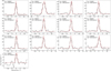Fig. B.1

Line profiles of the detected SO₂ transitions at the peak flux location of the 6_4,2-6_3,3 transition. The red line displays the fitted Gaussian line profile at the resolution of the spectrum (0.9 km s⁻¹), whereas the red dashed line shows the Gaussian line profile at a higher resolution. The lines are ordered based on their upper level energies (E_up).

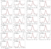Fig. B.2

Similar as Figure B.1, but for the detected CH₃OH transitions at the peak flux position of the 13₋₁-13₀ transition.

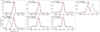Fig. B.3

Similar as Figure B.1, but for the detected H₂CO transitions at the peak flux position of the 5_0,5-4_0,4 transition.

Appendix C H₂CO line ratios

5_3,3-4_3,2/5_1,5-4_1,4: for the ortho-transition line pair, we see a clear spot (bright yellow) in the ratio map, where the ratios exceed those from the RADEX calculations. Therefore, the temperature derived for these pixels is limited by the upper range of 500 K. Ratios involving transitions with higher upper level energies are, therefore, needed to infer the temperature for these pixels. For the pixels for which the ratio does not exceed those from the calculations, we generally find temperatures, for both gas densities (and, therefore, across the vertical height of the disk), of the order of ~ 150-300 K. These are similar to and slightly higher than the derived temperatures for the disk-integrated fluxes of ~200 K inferred by van der Marel et al. (2021) (red line in the left panels). The peak pixel of the 5_0,5-4_0,4 transition is contained within the region of pixels that exceed the ratios from the RADEX calculations and the temperature is, therefore, not well constrained.

5_2,4-4_2,3/5_0,5-4_0,4: for this first para-transition line pair we find that the inferred ratios from the observations exceed the ratios obtained from the RADEX calculations. This is likely the result of the low upper level energies of the transitions involved, 100 K and 52 K, respectively, which are not sensitive to the higher temperatures ~ 150-350 K as probed by the ortho line pair.

5_4,2 -4_4,1 /5_0,5-4_0,4: for the second line pair, we find very similar results to the single ortho line pair. We find a spot in the centre of the maps that is limited by the temperature sensitivity of the lines. In addition, we find temperatures, for the other pixels, of the order of 150 K to 300 K for both gas densities. Those temperatures are, again, similar to those inferred for the disk-integrated fluxes by van der Marel et al. (2021). Once more, the peak position of the 5_0,5-4_0,4 transition falls within the range for which the temperature is not well constrained.

5_4,2 -4_4,1/5_2,4-4_2,3: for this final line pair, which involves the ratio of the transitions with the highest upper level energies (241 K and 100 K, respectively), we find similar results as for the ratio (5_4,2-4_4,1 /5_0,5-4_0,4) above, although we are able to provide better constraints on the temperature for a larger number of pixels. The temperature across the disk, especially when considering the gas density of $n_{H_{2}} = 10^{8}$ ${n_{{{\rm{H}}_2}}} = {10^8}$ cm⁻³, is of the order of 150 K to 350 K. Again, this is similar to or slightly higher than the dis-integrated one.

References

Aikawa, Y., van Zadelhoff, G. J., van Dishoeck, E. F., & Herbst, E. 2002, A&A, 386, 622 [NASA ADS] [CrossRef] [EDP Sciences] [Google Scholar]
Astropy Collaboration (Robitaille, T. P., et al.) 2013, A&A, 558, A33 [NASA ADS] [CrossRef] [EDP Sciences] [Google Scholar]
Astropy Collaboration (Price-Whelan, A. M., et al.) 2018, AJ, 156, 123 [Google Scholar]
Astropy Collaboration (Price-Whelan, A. M., et al.) 2022, ApJ, 935, 167 [NASA ADS] [CrossRef] [Google Scholar]
Atkinson, R., Baulch, D. L., Cox, R. A., et al. 2006, Atmos. Chem. Phys., 6, 3625 [NASA ADS] [CrossRef] [Google Scholar]
Balança, C., Spielfiedel, A., & Feautrier, N. 2016, MNRAS, 460, 3766 [CrossRef] [Google Scholar]
Banzatti, A., Meyer, M. R., Bruderer, S., et al. 2012, ApJ, 745, 90 [NASA ADS] [CrossRef] [Google Scholar]
Bergner, J. B., Guzmán, V. G., Oberg, K. I., Loomis, R. A., & Pegues, J. 2018, ApJ, 857, 69 [NASA ADS] [CrossRef] [Google Scholar]
Boehler, Y., Weaver, E., Isella, A., et al. 2017, ApJ, 840, 60 [Google Scholar]
Boehler, Y., Ménard, F., Robert, C. M. T., et al. 2021, A&A, 650, A59 [NASA ADS] [CrossRef] [EDP Sciences] [Google Scholar]
Booth, A. S., van der Marel, N., Leemker, M., van Dishoeck, E. F., & Ohashi, S. 2021, A&A, 651, L6 [NASA ADS] [CrossRef] [EDP Sciences] [Google Scholar]
Booth, A. S., Law, C. J., Temmink, M., Leemker, M., & Macías, E. 2023, A&A, 678, A146 [NASA ADS] [CrossRef] [EDP Sciences] [Google Scholar]
Booth, A. S., Temmink, M., van Dishoeck, E. F., et al. 2024, AJ, 167, 165 [NASA ADS] [CrossRef] [Google Scholar]
Bosman, A. D., Bergin, E. A., Loomis, R. A., et al. 2021, ApJS, 257, 15 [NASA ADS] [CrossRef] [Google Scholar]
Brown, W. A., & Bolina, A. S. 2007, MNRAS, 374, 1006 [NASA ADS] [CrossRef] [Google Scholar]
Brown, J. M., Herczeg, G. J., Pontoppidan, K. M., & van Dishoeck, E. F. 2012, ApJ, 744, 116 [Google Scholar]
Bruderer, S. 2013, A&A, 559, A46 [NASA ADS] [CrossRef] [EDP Sciences] [Google Scholar]
Bruderer, S., van Dishoeck, E. F., Doty, S. D., & Herczeg, G. J. 2012, A&A, 541, A91 [NASA ADS] [CrossRef] [EDP Sciences] [Google Scholar]
Bruderer, S., van der Marel, N., van Dishoeck, E. F., & van Kempen, T. A. 2014, A&A, 562, A26 [NASA ADS] [CrossRef] [EDP Sciences] [Google Scholar]
Brunken, N. G. C., Booth, A. S., Leemker, M., et al. 2022, A&A, 659, A29 [NASA ADS] [CrossRef] [EDP Sciences] [Google Scholar]
Carney, M. T., Hogerheijde, M. R., Loomis, R. A., et al. 2017, A&A, 605, A21 [NASA ADS] [CrossRef] [EDP Sciences] [Google Scholar]
Carney, M. T., Fedele, D., Hogerheijde, M. R., et al. 2018, A&A, 614, A106 [NASA ADS] [CrossRef] [EDP Sciences] [Google Scholar]
Carney, M. T., Hogerheijde, M. R., Guzmán, V. V., et al. 2019, A&A, 623, A124 [NASA ADS] [CrossRef] [EDP Sciences] [Google Scholar]
Cleeves, L. I., Loomis, R. A., Teague, R., et al. 2021, ApJ, 911, 29 [NASA ADS] [CrossRef] [Google Scholar]
Crnkovic-Rubsamen, I., Zhu, Z., & Stone, J. M. 2015, MNRAS, 450, 4285 [NASA ADS] [CrossRef] [Google Scholar]
D’Alessio, P., Cantö, J., Calvet, N., & Lizano, S. 1998, ApJ, 500, 411 [Google Scholar]
Dartois, E., Dutrey, A., & Guilloteau, S. 2003, A&A, 399, 773 [CrossRef] [EDP Sciences] [Google Scholar]
Facchini, S., Birnstiel, T., Bruderer, S., & van Dishoeck, E. F. 2017, A&A, 605, A16 [NASA ADS] [CrossRef] [EDP Sciences] [Google Scholar]
Flaherty, K., Hughes, A. M., Simon, J. B., et al. 2020, ApJ, 895, 109 [NASA ADS] [CrossRef] [Google Scholar]
Flaherty, K., Hughes, A. M., Simon, J. B., et al. 2024, MNRAS, 532, 363 [NASA ADS] [CrossRef] [Google Scholar]
Flock, M., Nelson, R. P., Turner, N. J., et al. 2017, ApJ, 850, 131 [Google Scholar]
Flock, M., Turner, N. J., Nelson, R. P., et al. 2020, ApJ, 897, 155 [Google Scholar]
Fockenberg, C., & Preses, J. M. 2002, J. Phys. Chem. A, 106, 2924 [NASA ADS] [CrossRef] [Google Scholar]
Francis, L., & van der Marel, N. 2020, ApJ, 892, 111 [Google Scholar]
Fuchs, G. W., Cuppen, H. M., Ioppolo, S., et al. 2009, A&A, 505, 629 [NASA ADS] [CrossRef] [EDP Sciences] [Google Scholar]
Furuya, K. 2024, ApJ, 974, 115 [NASA ADS] [CrossRef] [Google Scholar]
Gaia Collaboration (Brown, A. G. A., et al.) 2018, A&A, 616, A1 [NASA ADS] [CrossRef] [EDP Sciences] [Google Scholar]
Goldsmith, P. F., & Langer, W. D. 1999, ApJ, 517, 209 [Google Scholar]
Guzmán, V. V., Oberg, K. I., Carpenter, J., et al. 2018, ApJ, 864, 170 [CrossRef] [Google Scholar]
Hammer, M., & Lin, M.-K. 2023, MNRAS, 525, 123 [NASA ADS] [CrossRef] [Google Scholar]
Hammer, M., Kratter, K. M., & Lin, M.-K. 2017, MNRAS, 466, 3533 [NASA ADS] [CrossRef] [Google Scholar]
Hammer, M., Pinilla, P., Kratter, K. M., & Lin, M.-K. 2019, MNRAS, 482, 3609 [NASA ADS] [CrossRef] [Google Scholar]
Hammer, M., Lin, M.-K., Kratter, K. M., & Pinilla, P. 2021, MNRAS, 504, 3963 [NASA ADS] [CrossRef] [Google Scholar]
Harris, C. R., Millman, K. J., van der Walt, S. J., et al. 2020, Nature, 585, 357 [NASA ADS] [CrossRef] [Google Scholar]
Harsono, D., Bruderer, S., & van Dishoeck, E. F. 2015, A&A, 582, A41 [NASA ADS] [CrossRef] [EDP Sciences] [Google Scholar]
Hartmann, L., Calvet, N., Gullbring, E., & D’Alessio, P. 1998, ApJ, 495, 385 [Google Scholar]
Hasegawa, T. I., Herbst, E., & Leung, C. M. 1992, ApJS, 82, 167 [Google Scholar]
Heays, A. N., Bosman, A. D., & van Dishoeck, E. F. 2017, A&A, 602, A105 [NASA ADS] [CrossRef] [EDP Sciences] [Google Scholar]
Herbst, E., & van Dishoeck, E. F. 2009, ARA&A, 47, 427 [NASA ADS] [CrossRef] [Google Scholar]
Hernández-Vera, C., Guzmán, V. V., Artur de la Villarmois, E., et al. 2024, ApJ, 967, 68 [CrossRef] [Google Scholar]
Huang, P., Isella, A., Li, H., Li, S., & Ji, J. 2018, ApJ, 867, 3 [NASA ADS] [CrossRef] [Google Scholar]
Hunter, J. D. 2007, Comput. Sci. Eng., 9, 90 [NASA ADS] [CrossRef] [Google Scholar]
Ilee, J. D., Walsh, C., Booth, A. S., et al. 2021, ApJS, 257, 9 [NASA ADS] [CrossRef] [Google Scholar]
Isella, A., Huang, J., Andrews, S. M., et al. 2018, ApJ, 869, L49 [NASA ADS] [CrossRef] [Google Scholar]
Johnstone, D., Boonman, A. M. S., & van Dishoeck, E. F. 2003, A&A, 412, 157 [NASA ADS] [CrossRef] [EDP Sciences] [Google Scholar]
Kama, M., Bruderer, S., van Dishoeck, E. F., et al. 2016, A&A, 592, A83 [NASA ADS] [CrossRef] [EDP Sciences] [Google Scholar]
Kayanuma, M., Shoji, M., Furuya, K., et al. 2019, Chem. Phys. Lett., 714, 137 [NASA ADS] [CrossRef] [Google Scholar]
Kluyver, T., Ragan-Kelley, B., Pérez, F., et al. 2016, in Positioning and Power in Academic Publishing: Players, Agents and Agendas, eds. F. Loizides, & B. Schmidt (IOS Press), 87 [Google Scholar]
Law, C. J., Teague, R., Loomis, R. A., et al. 2021, ApJS, 257, 4 [NASA ADS] [CrossRef] [Google Scholar]
Law, C. J., Alarcón, F., Cleeves, L. I., Oberg, K. I., & Paneque-Carreño, T. 2023a, ApJ, 959, L27 [NASA ADS] [CrossRef] [Google Scholar]
Law, C. J., Teague, R., Oberg, K. I., et al. 2023b, ApJ, 948, 60 [NASA ADS] [CrossRef] [Google Scholar]
Law, C. J., Benisty, M., Facchini, S., et al. 2024, ApJ, 964, 190 [NASA ADS] [CrossRef] [Google Scholar]
Le Gal, R., Oberg, K. I., Loomis, R. A., Pegues, J., & Bergner, J. B. 2019, ApJ, 876, 72 [NASA ADS] [CrossRef] [Google Scholar]
Le Gal, R., Oberg, K. I., Teague, R., et al. 2021, ApJS, 257, 12 [NASA ADS] [CrossRef] [Google Scholar]
Leemker, M., van’t Hoff, M. L. R., Trapman, L., et al. 2021, A&A, 646, A3 [EDP Sciences] [Google Scholar]
Leemker, M., Booth, A. S., van Dishoeck, E. F., et al. 2022, A&A, 663, A23 [NASA ADS] [CrossRef] [EDP Sciences] [Google Scholar]
Leemker, M., Booth, A. S., van Dishoeck, E. F., et al. 2023, A&A, 673, A7 [NASA ADS] [CrossRef] [EDP Sciences] [Google Scholar]
Li, H., Finn, J. M., Lovelace, R. V. E., & Colgate, S. A. 2000, ApJ, 533, 1023 [NASA ADS] [CrossRef] [Google Scholar]
Loomis, R. A., Cleeves, L. I., Oberg, K. I., Guzman, V. V., & Andrews, S. M. 2015, ApJ, 809, L25 [NASA ADS] [CrossRef] [Google Scholar]
Loomis, R. A., Cleeves, L. I., Oberg, K. I., et al. 2018, ApJ, 859, 131 [NASA ADS] [CrossRef] [Google Scholar]
Lovelace, R. V. E., & Hohlfeld, R. G. 2013, MNRAS, 429, 529 [NASA ADS] [CrossRef] [Google Scholar]
Lovelace, R. V. E., & Romanova, M. M. 2014, Fluid Dyn. Res., 46, 041401 [NASA ADS] [CrossRef] [Google Scholar]
Lovelace, R. V. E., Li, H., Colgate, S. A., & Nelson, A. F. 1999, ApJ, 513, 805 [NASA ADS] [CrossRef] [Google Scholar]
Lynden-Bell, D., & Pringle, J. E. 1974, MNRAS, 168, 603 [Google Scholar]
Lyra, W., Johansen, A., Zsom, A., Klahr, H., & Piskunov, N. 2009, A&A, 497, 869 [NASA ADS] [CrossRef] [EDP Sciences] [Google Scholar]
Meheut, H., Meliani, Z., Varniere, P., & Benz, W. 2012a, A&A, 545, A134 [NASA ADS] [CrossRef] [EDP Sciences] [Google Scholar]
Meheut, H., Yu, C., & Lai, D. 2012b, MNRAS, 422, 2399 [NASA ADS] [CrossRef] [Google Scholar]
Meheut, H., Lovelace, R. V. E., & Lai, D. 2013, MNRAS, 430, 1988 [NASA ADS] [CrossRef] [Google Scholar]
Minissale, M., Aikawa, Y., Bergin, E., et al. 2022, ACS Earth Space Chem., 6, 597 [NASA ADS] [CrossRef] [Google Scholar]
Muñoz-Romero, C. E., Oberg, K. I., Law, C. J., et al. 2023, ApJ, 943, 35 [CrossRef] [Google Scholar]
Müller, H. S. P., Thorwirth, S., Roth, D. A., & Winnewisser, G. 2001, A&A, 370, L49 [Google Scholar]
Nazari, P., Tabone, B., & Rosotti, G. P. 2023, A&A, 671, A107 [NASA ADS] [CrossRef] [EDP Sciences] [Google Scholar]
Noble, J. A., Theule, P., Mispelaer, F., et al. 2012, A&A, 543, A5 [NASA ADS] [CrossRef] [EDP Sciences] [Google Scholar]
Öberg, K. I., & Bergin, E. A. 2021, Phys. Rep., 893, 1 [Google Scholar]
Öberg, K. I., Facchini, S., & Anderson, D. E. 2023, ARA&A, 61, 287 [CrossRef] [Google Scholar]
Ohashi, S., Kataoka, A., van der Marel, N., et al. 2020, ApJ, 900, 81 [Google Scholar]
Owen, J. E., & Kollmeier, J. A. 2017, MNRAS, 467, 3379 [NASA ADS] [CrossRef] [Google Scholar]
Paneque-Carreño, T., Miotello, A., van Dishoeck, E. F., et al. 2023, A&A, 669, A126 [NASA ADS] [CrossRef] [EDP Sciences] [Google Scholar]
Paneque-Carreño, T., Izquierdo, A. F., Teague, R., et al. 2024, A&A, 684, A174 [NASA ADS] [CrossRef] [EDP Sciences] [Google Scholar]
Pegues, J., Oberg, K. I., Bergner, J. B., et al. 2020, ApJ, 890, 142 [NASA ADS] [CrossRef] [Google Scholar]
Penteado, E. M., Walsh, C., & Cuppen, H. M. 2017, ApJ, 844, 71 [Google Scholar]
Pérez, F., & Granger, B. E. 2007, Comput. Sci. Eng., 9, 21 [Google Scholar]
Perrero, J., Enrique-Romero, J., Ferrero, S., et al. 2022, ApJ, 938, 158 [NASA ADS] [CrossRef] [Google Scholar]
Rab, C., Kamp, I., Dominik, C., et al. 2020, A&A, 642, A165 [EDP Sciences] [Google Scholar]
Rabli, D., & Flower, D. R. 2010, MNRAS, 406, 95 [Google Scholar]
Raettig, N., Lyra, W., & Klahr, H. 2021, ApJ, 913, 92 [NASA ADS] [CrossRef] [Google Scholar]
Rampinelli, L., Facchini, S., Leemker, M., et al. 2024, A&A, 689, A65 [NASA ADS] [CrossRef] [EDP Sciences] [Google Scholar]
Regály, Z., Kadam, K., & Dullemond, C. P. 2021, MNRAS, 506, 2685 [CrossRef] [Google Scholar]
Rosotti, G. P., Ilee, J. D., Facchini, S., et al. 2021, MNRAS, 501, 3427 [Google Scholar]
Salinas, V. N., Hogerheijde, M. R., Mathews, G. S., et al. 2017, A&A, 606, A125 [NASA ADS] [CrossRef] [EDP Sciences] [Google Scholar]
Santos, J. C., Chuang, K.-J., Lamberts, T., et al. 2022, ApJ, 931, L33 [NASA ADS] [CrossRef] [Google Scholar]
Savitzky, A., & Golay, M. J. E. 1964, Analyt. Chem., 36, 1627 [NASA ADS] [CrossRef] [Google Scholar]
Schöier, F. L., van der Tak, F. F. S., van Dishoeck, E. F., & Black, J. H. 2005, A&A, 432, 369 [Google Scholar]
Semenov, D., Wiebe, D., & Henning, T. 2006, ApJ, 647, L57 [NASA ADS] [CrossRef] [Google Scholar]
Stapper, L. M., Hogerheijde, M. R., van Dishoeck, E. F., et al. 2024, A&A, 682, A149 [NASA ADS] [CrossRef] [EDP Sciences] [Google Scholar]
Temmink, M., Booth, A. S., van der Marel, N., & van Dishoeck, E. F. 2023, A&A, 675, A131 [NASA ADS] [CrossRef] [EDP Sciences] [Google Scholar]
Terwisscha van Scheltinga, J., Hogerheijde, M. R., Cleeves, L. I., et al. 2021, ApJ, 906, 111 [Google Scholar]
Terwisscha van Scheltinga, J., Ligterink, N. F. W., Bosman, A. D., Hogerheijde, M. R., & Linnartz, H. 2022, A&A, 666, A35 [NASA ADS] [CrossRef] [EDP Sciences] [Google Scholar]
The pandas development team 2020, https://doi.org/10.5281/zenodo.3509134 [Google Scholar]
Thi, W. F., van Zadelhoff, G. J., & van Dishoeck, E. F. 2004, A&A, 425, 955 [NASA ADS] [CrossRef] [EDP Sciences] [Google Scholar]
Tielens, A. G. G. M., & Allamandola, L. J. 1987, in Interstellar Processes, 134, eds. D. J. Hollenbach, J. Thronson, & A. Harley, 397 [NASA ADS] [CrossRef] [Google Scholar]
Urbina, F., Miley, J., Kama, M., & Keyte, L. 2024, A&A, 686, A120 [NASA ADS] [CrossRef] [EDP Sciences] [Google Scholar]
van der Marel, N., van Dishoeck, E. F., Bruderer, S., et al. 2013, Science, 340, 1199 [Google Scholar]
van der Marel, N., van Dishoeck, E. F., Bruderer, S., & van Kempen, T. A. 2014, A&A, 563, A113 [NASA ADS] [CrossRef] [EDP Sciences] [Google Scholar]
van der Marel, N., van Dishoeck, E. F., Bruderer, S., et al. 2016, A&A, 585, A58 [NASA ADS] [CrossRef] [EDP Sciences] [Google Scholar]
van der Marel, N., Booth, A. S., Leemker, M., van Dishoeck, E. F., & Ohashi, S. 2021, A&A, 651, L5 [NASA ADS] [CrossRef] [EDP Sciences] [Google Scholar]
van der Tak, F. F. S., Black, J. H., Schöier, F. L., Jansen, D. J., & van Dishoeck, E. F. 2007, A&A, 468, 627 [NASA ADS] [CrossRef] [EDP Sciences] [Google Scholar]
van Zadelhoff, G. J., van Dishoeck, E. F., Thi, W. F., & Blake, G. A. 2001, A&A, 377, 566 [NASA ADS] [CrossRef] [EDP Sciences] [Google Scholar]
van Zadelhoff, G. J., Aikawa, Y., Hogerheijde, M. R., & van Dishoeck, E. F. 2003, A&A, 397, 789 [CrossRef] [EDP Sciences] [Google Scholar]
Virtanen, P., Gommers, R., Oliphant, T. E., et al. 2020, Nature Methods, 17, 261 [CrossRef] [Google Scholar]
Walsh, C., Millar, T. J., & Nomura, H. 2010, ApJ, 722, 1607 [Google Scholar]
Watanabe, N., & Kouchi, A. 2002, ApJ, 571, L173 [Google Scholar]
Weaver, E., Isella, A., & Boehler, Y. 2018, ApJ, 853, 113 [Google Scholar]
Wiesenfeld, L., & Faure, A. 2013, MNRAS, 432, 2573 [NASA ADS] [CrossRef] [Google Scholar]
Woitke, P., Kamp, I., & Thi, W. F. 2009, A&A, 501, 383 [NASA ADS] [CrossRef] [EDP Sciences] [Google Scholar]
Xie, T., Allen, M., & Langer, W. D. 1995, ApJ, 440, 674 [NASA ADS] [CrossRef] [Google Scholar]
Yang, H., Fernández-López, M., Li, Z.-Y., et al. 2023, ApJ, 948, L2 [NASA ADS] [CrossRef] [Google Scholar]
Yang, H., Fernández-López, M., Li, Z.-Y., et al. 2024, ApJ, 963, 134 [NASA ADS] [CrossRef] [Google Scholar]
Youdin, A. N., & Lithwick, Y. 2007, Icarus, 192, 588 [NASA ADS] [CrossRef] [Google Scholar]

All Tables

Table A.1

Detected transitions of SO₂ (top part), CH₃OH (middle part), and H₂CO (bottom part).

In the text

Table A.2

All removed transitions due to blending and/or noise.

In the text

All Figures

Fig. 1

Dust continuum (top left; Yang et al. 2023) and moment-0 maps of the ¹³CO.J=3−2 (top centre; Leemker et al. 2023) and .J=6−5 (top right; van der Marel et al. 2016), and the SO₂ J=6_4,2–6_3,3 (bottom left), CH₃OH J=13₋₁−13₀ (bottom centre), and H₂CO J=5_0,5−4_0,4 (bottom right) transitions. The white star in the centre indicates the approximate location of the host star, whereas the resolving beam is indicated in the lower left. The red circle and cross provide, respectively, the peak flux position of the SO₂ and CH₃OH transitions in the bottom left and centre plots, whereas the red square denotes the peak flux position of the H₂CO transition in the bottom right plot. In addition, the arrows in the ¹³CO .J=3−2 transition indicate where the emission is affected by the cloud absorption.

In the text

	Fig. 2 Rotational diagrams for SO₂ (left) and CH₃OH (right) at the peak flux positions of their 6_4,2−6_3,3 and 13₋₁−13₀ transitions, respectively. The colour bar indicates the value for A_ul (×10⁻⁴) of the transitions.
In the text

	Fig. 3 Temperature (left column), column density (middle column), and maximum optical depth (right column) maps for SO₂ (top) and CH₃OH (bottom).
In the text

Fig. 4

Line ratios for the different pairs of H₂CO transitions. The left panels show the RADEX calculations, with the colour map indicating the various ratios. The white contours indicate the values of 0.3, 0.5, and 0.7, whereas the red contour indicates the disk integrated ratio from van der Marel et al. (2021). The panels in the second column indicate the ratios derived for the pixels where both transitions are detected, using the colour scheme as for the left panels. The final two columns display the derived temperatures for gas densities of $n_{H_{2}} = 10^{7} {cm}^{- 3}$ ${n_{{{\rm{H}}_2}}} = {10^7}{\rm{c}}{{\rm{m}}^{ - 3}}$ (representative of the disk’s atmosphere, z/r ≳0.2) and 10⁸ cm⁻³ (representative of the disk’s midplane). The white solid, dashed, and dotted contours indicate temperatures of 200 K, 300 K, and 400 K, respectively.

In the text

Fig. 5

RADEX grids for SO₂ (top panel), A- and E-type CH₃OH (second and third panels), and ortho- and para-H₂CO (bottom two panels) showing the percentile difference between the kinetic and rotational temperature (∆T), as a measure of thermalised transitions. The contours (solid, dashed, and dashed-dotted) in each panel indicates when ∆T=1%, 5%, and 10%, respectively. Above these contours the lines will be thermalised. The white shaded area indicates the gas density of the dust trap according to the DALI model (Leemker et al. 2023). Finally, the arrows indicate the derived excitation temperatures of T ~ 55 K for SO₂ and T ~ 130 K for CH₃OH. For H₂CO we show the rotational temperature of 150 K, the lower value of the inferred temperature range.

In the text

	Fig. 6 Cartoon visualising the expected effect of the vortex on the temperature structure. Hotter gas, due to UV heating, will be counteracted by colder gas being brought in due to the potential vortex motions, which primarily acts in the midplane. This effect is not observed in the IRS 48 disk, unless the temperatures variations are very small.
In the text

	Fig. 7 Brightness temperature maps of the dust continuum (left) and the ¹³CO .J=3−2 (middle panel) and ¹³CO .J=6−5 (right panel) transitions. The yellow stars in the centre indicate the approximate location of the host star, while the resolving beams are indicated by the white ellipses.
In the text

Fig. 8

Optical depth (given in log₁₀-space) grids for a range of beam radii (assuming circular beams) and turbulent line widths (∆V) for SO₂ J=6_4,2−6_3,3 (at T_rot=55 K), CH₃OH 7=13₋₁−13₀ (at T_rot=150 K, accounting for the underestimation of the temperature due to sub-thermal excitation), and H₂CO J=5_1,5−4_1,4 (at T_rot=150 K and T_rot=350 K). The contour lines indicate values of τ=1, 10, and 100. The dotted black line indicates the radial FWHM of the dust trap (FWHM_dust ≃ 26.5 au), found using the high-resolution observations of Yang et al. (2023). The vertical dashed line indicates a turbulent line width of ∆V_line=0.2 km s⁻¹, the lower value used in our analysis.

In the text

	Fig. 9 Cartoon visualising our proposed radial vertical emission scheme, containing SO₂ (blue), ¹³CO (orange), and H₂CO and CH₃OH (red). The radial and vertical emission locations are based on the derived temperatures, the proposed sliver theory, and the assumption that the ¹³CO emission is spatially resolved.
In the text

Fig. 10

Zoom-in of the model structure of the dust trap region of the IRS 48 disk of the gas density (n_gas in cm⁻³, left panel) and gas and dust temperature (both in Kelvin, left and right panels, respectively). The vertical bars indicate the location of the dust trap, extending from 60 to 80 au, while the white contours in the left most panel indicate gas densities between 10⁷ and 10⁸ cm⁻³. The images have been adapted from Leemker et al. (2023).

In the text

	Fig. B.1 Line profiles of the detected SO₂ transitions at the peak flux location of the 6_4,2-6_3,3 transition. The red line displays the fitted Gaussian line profile at the resolution of the spectrum (0.9 km s⁻¹), whereas the red dashed line shows the Gaussian line profile at a higher resolution. The lines are ordered based on their upper level energies (E_up).
In the text

	Fig. B.2 Similar as Figure B.1, but for the detected CH₃OH transitions at the peak flux position of the 13₋₁-13₀ transition.
In the text

	Fig. B.3 Similar as Figure B.1, but for the detected H₂CO transitions at the peak flux position of the 5_0,5-4_0,4 transition.
In the text

Current usage metrics show cumulative count of Article Views (full-text article views including HTML views, PDF and ePub downloads, according to the available data) and Abstracts Views on Vision4Press platform.

Data correspond to usage on the plateform after 2015. The current usage metrics is available 48-96 hours after online publication and is updated daily on week days.

Initial download of the metrics may take a while.

[1] Aikawa, Y., van Zadelhoff, G. J., van Dishoeck, E. F., & Herbst, E. 2002, A&A, 386, 622 [NASA ADS] [CrossRef] [EDP Sciences] [Google Scholar]

[2] Astropy Collaboration (Robitaille, T. P., et al.) 2013, A&A, 558, A33 [NASA ADS] [CrossRef] [EDP Sciences] [Google Scholar]

[3] Astropy Collaboration (Price-Whelan, A. M., et al.) 2018, AJ, 156, 123 [Google Scholar]

[4] Astropy Collaboration (Price-Whelan, A. M., et al.) 2022, ApJ, 935, 167 [NASA ADS] [CrossRef] [Google Scholar]

[5] Atkinson, R., Baulch, D. L., Cox, R. A., et al. 2006, Atmos. Chem. Phys., 6, 3625 [NASA ADS] [CrossRef] [Google Scholar]

[6] Balança, C., Spielfiedel, A., & Feautrier, N. 2016, MNRAS, 460, 3766 [CrossRef] [Google Scholar]

[7] Banzatti, A., Meyer, M. R., Bruderer, S., et al. 2012, ApJ, 745, 90 [NASA ADS] [CrossRef] [Google Scholar]

[8] Bergner, J. B., Guzmán, V. G., Oberg, K. I., Loomis, R. A., & Pegues, J. 2018, ApJ, 857, 69 [NASA ADS] [CrossRef] [Google Scholar]

[9] Boehler, Y., Weaver, E., Isella, A., et al. 2017, ApJ, 840, 60 [Google Scholar]

[10] Boehler, Y., Ménard, F., Robert, C. M. T., et al. 2021, A&A, 650, A59 [NASA ADS] [CrossRef] [EDP Sciences] [Google Scholar]

[11] Booth, A. S., van der Marel, N., Leemker, M., van Dishoeck, E. F., & Ohashi, S. 2021, A&A, 651, L6 [NASA ADS] [CrossRef] [EDP Sciences] [Google Scholar]

[12] Booth, A. S., Law, C. J., Temmink, M., Leemker, M., & Macías, E. 2023, A&A, 678, A146 [NASA ADS] [CrossRef] [EDP Sciences] [Google Scholar]

[13] Booth, A. S., Temmink, M., van Dishoeck, E. F., et al. 2024, AJ, 167, 165 [NASA ADS] [CrossRef] [Google Scholar]

[14] Bosman, A. D., Bergin, E. A., Loomis, R. A., et al. 2021, ApJS, 257, 15 [NASA ADS] [CrossRef] [Google Scholar]

[15] Brown, W. A., & Bolina, A. S. 2007, MNRAS, 374, 1006 [NASA ADS] [CrossRef] [Google Scholar]

[16] Brown, J. M., Herczeg, G. J., Pontoppidan, K. M., & van Dishoeck, E. F. 2012, ApJ, 744, 116 [Google Scholar]

[17] Bruderer, S. 2013, A&A, 559, A46 [NASA ADS] [CrossRef] [EDP Sciences] [Google Scholar]

[18] Bruderer, S., van Dishoeck, E. F., Doty, S. D., & Herczeg, G. J. 2012, A&A, 541, A91 [NASA ADS] [CrossRef] [EDP Sciences] [Google Scholar]

[19] Bruderer, S., van der Marel, N., van Dishoeck, E. F., & van Kempen, T. A. 2014, A&A, 562, A26 [NASA ADS] [CrossRef] [EDP Sciences] [Google Scholar]

[20] Brunken, N. G. C., Booth, A. S., Leemker, M., et al. 2022, A&A, 659, A29 [NASA ADS] [CrossRef] [EDP Sciences] [Google Scholar]

[21] Carney, M. T., Hogerheijde, M. R., Loomis, R. A., et al. 2017, A&A, 605, A21 [NASA ADS] [CrossRef] [EDP Sciences] [Google Scholar]

[22] Carney, M. T., Fedele, D., Hogerheijde, M. R., et al. 2018, A&A, 614, A106 [NASA ADS] [CrossRef] [EDP Sciences] [Google Scholar]

[23] Carney, M. T., Hogerheijde, M. R., Guzmán, V. V., et al. 2019, A&A, 623, A124 [NASA ADS] [CrossRef] [EDP Sciences] [Google Scholar]

[24] Cleeves, L. I., Loomis, R. A., Teague, R., et al. 2021, ApJ, 911, 29 [NASA ADS] [CrossRef] [Google Scholar]

[25] Crnkovic-Rubsamen, I., Zhu, Z., & Stone, J. M. 2015, MNRAS, 450, 4285 [NASA ADS] [CrossRef] [Google Scholar]

[26] D’Alessio, P., Cantö, J., Calvet, N., & Lizano, S. 1998, ApJ, 500, 411 [Google Scholar]

[27] Dartois, E., Dutrey, A., & Guilloteau, S. 2003, A&A, 399, 773 [CrossRef] [EDP Sciences] [Google Scholar]

[28] Facchini, S., Birnstiel, T., Bruderer, S., & van Dishoeck, E. F. 2017, A&A, 605, A16 [NASA ADS] [CrossRef] [EDP Sciences] [Google Scholar]

[29] Flaherty, K., Hughes, A. M., Simon, J. B., et al. 2020, ApJ, 895, 109 [NASA ADS] [CrossRef] [Google Scholar]

[30] Flaherty, K., Hughes, A. M., Simon, J. B., et al. 2024, MNRAS, 532, 363 [NASA ADS] [CrossRef] [Google Scholar]

[31] Flock, M., Nelson, R. P., Turner, N. J., et al. 2017, ApJ, 850, 131 [Google Scholar]

[32] Flock, M., Turner, N. J., Nelson, R. P., et al. 2020, ApJ, 897, 155 [Google Scholar]

[33] Fockenberg, C., & Preses, J. M. 2002, J. Phys. Chem. A, 106, 2924 [NASA ADS] [CrossRef] [Google Scholar]

[34] Francis, L., & van der Marel, N. 2020, ApJ, 892, 111 [Google Scholar]

[35] Fuchs, G. W., Cuppen, H. M., Ioppolo, S., et al. 2009, A&A, 505, 629 [NASA ADS] [CrossRef] [EDP Sciences] [Google Scholar]

[36] Furuya, K. 2024, ApJ, 974, 115 [NASA ADS] [CrossRef] [Google Scholar]

[37] Gaia Collaboration (Brown, A. G. A., et al.) 2018, A&A, 616, A1 [NASA ADS] [CrossRef] [EDP Sciences] [Google Scholar]

[38] Goldsmith, P. F., & Langer, W. D. 1999, ApJ, 517, 209 [Google Scholar]

[39] Guzmán, V. V., Oberg, K. I., Carpenter, J., et al. 2018, ApJ, 864, 170 [CrossRef] [Google Scholar]

[40] Hammer, M., & Lin, M.-K. 2023, MNRAS, 525, 123 [NASA ADS] [CrossRef] [Google Scholar]

[41] Hammer, M., Kratter, K. M., & Lin, M.-K. 2017, MNRAS, 466, 3533 [NASA ADS] [CrossRef] [Google Scholar]

[42] Hammer, M., Pinilla, P., Kratter, K. M., & Lin, M.-K. 2019, MNRAS, 482, 3609 [NASA ADS] [CrossRef] [Google Scholar]

[43] Hammer, M., Lin, M.-K., Kratter, K. M., & Pinilla, P. 2021, MNRAS, 504, 3963 [NASA ADS] [CrossRef] [Google Scholar]

[44] Harris, C. R., Millman, K. J., van der Walt, S. J., et al. 2020, Nature, 585, 357 [NASA ADS] [CrossRef] [Google Scholar]

[45] Harsono, D., Bruderer, S., & van Dishoeck, E. F. 2015, A&A, 582, A41 [NASA ADS] [CrossRef] [EDP Sciences] [Google Scholar]

[46] Hartmann, L., Calvet, N., Gullbring, E., & D’Alessio, P. 1998, ApJ, 495, 385 [Google Scholar]

[47] Hasegawa, T. I., Herbst, E., & Leung, C. M. 1992, ApJS, 82, 167 [Google Scholar]

[48] Heays, A. N., Bosman, A. D., & van Dishoeck, E. F. 2017, A&A, 602, A105 [NASA ADS] [CrossRef] [EDP Sciences] [Google Scholar]

[49] Herbst, E., & van Dishoeck, E. F. 2009, ARA&A, 47, 427 [NASA ADS] [CrossRef] [Google Scholar]

[50] Hernández-Vera, C., Guzmán, V. V., Artur de la Villarmois, E., et al. 2024, ApJ, 967, 68 [CrossRef] [Google Scholar]

[51] Huang, P., Isella, A., Li, H., Li, S., & Ji, J. 2018, ApJ, 867, 3 [NASA ADS] [CrossRef] [Google Scholar]

[52] Hunter, J. D. 2007, Comput. Sci. Eng., 9, 90 [NASA ADS] [CrossRef] [Google Scholar]

[53] Ilee, J. D., Walsh, C., Booth, A. S., et al. 2021, ApJS, 257, 9 [NASA ADS] [CrossRef] [Google Scholar]

[54] Isella, A., Huang, J., Andrews, S. M., et al. 2018, ApJ, 869, L49 [NASA ADS] [CrossRef] [Google Scholar]

[55] Johnstone, D., Boonman, A. M. S., & van Dishoeck, E. F. 2003, A&A, 412, 157 [NASA ADS] [CrossRef] [EDP Sciences] [Google Scholar]

[56] Kama, M., Bruderer, S., van Dishoeck, E. F., et al. 2016, A&A, 592, A83 [NASA ADS] [CrossRef] [EDP Sciences] [Google Scholar]

[57] Kayanuma, M., Shoji, M., Furuya, K., et al. 2019, Chem. Phys. Lett., 714, 137 [NASA ADS] [CrossRef] [Google Scholar]

[58] Kluyver, T., Ragan-Kelley, B., Pérez, F., et al. 2016, in Positioning and Power in Academic Publishing: Players, Agents and Agendas, eds. F. Loizides, & B. Schmidt (IOS Press), 87 [Google Scholar]

[59] Law, C. J., Teague, R., Loomis, R. A., et al. 2021, ApJS, 257, 4 [NASA ADS] [CrossRef] [Google Scholar]

[60] Law, C. J., Alarcón, F., Cleeves, L. I., Oberg, K. I., & Paneque-Carreño, T. 2023a, ApJ, 959, L27 [NASA ADS] [CrossRef] [Google Scholar]

[61] Law, C. J., Teague, R., Oberg, K. I., et al. 2023b, ApJ, 948, 60 [NASA ADS] [CrossRef] [Google Scholar]

[62] Law, C. J., Benisty, M., Facchini, S., et al. 2024, ApJ, 964, 190 [NASA ADS] [CrossRef] [Google Scholar]

[63] Le Gal, R., Oberg, K. I., Loomis, R. A., Pegues, J., & Bergner, J. B. 2019, ApJ, 876, 72 [NASA ADS] [CrossRef] [Google Scholar]

[64] Le Gal, R., Oberg, K. I., Teague, R., et al. 2021, ApJS, 257, 12 [NASA ADS] [CrossRef] [Google Scholar]

[65] Leemker, M., van’t Hoff, M. L. R., Trapman, L., et al. 2021, A&A, 646, A3 [EDP Sciences] [Google Scholar]

[66] Leemker, M., Booth, A. S., van Dishoeck, E. F., et al. 2022, A&A, 663, A23 [NASA ADS] [CrossRef] [EDP Sciences] [Google Scholar]

[67] Leemker, M., Booth, A. S., van Dishoeck, E. F., et al. 2023, A&A, 673, A7 [NASA ADS] [CrossRef] [EDP Sciences] [Google Scholar]

[68] Li, H., Finn, J. M., Lovelace, R. V. E., & Colgate, S. A. 2000, ApJ, 533, 1023 [NASA ADS] [CrossRef] [Google Scholar]

[69] Loomis, R. A., Cleeves, L. I., Oberg, K. I., Guzman, V. V., & Andrews, S. M. 2015, ApJ, 809, L25 [NASA ADS] [CrossRef] [Google Scholar]

[70] Loomis, R. A., Cleeves, L. I., Oberg, K. I., et al. 2018, ApJ, 859, 131 [NASA ADS] [CrossRef] [Google Scholar]

[71] Lovelace, R. V. E., & Hohlfeld, R. G. 2013, MNRAS, 429, 529 [NASA ADS] [CrossRef] [Google Scholar]

[72] Lovelace, R. V. E., & Romanova, M. M. 2014, Fluid Dyn. Res., 46, 041401 [NASA ADS] [CrossRef] [Google Scholar]

[73] Lovelace, R. V. E., Li, H., Colgate, S. A., & Nelson, A. F. 1999, ApJ, 513, 805 [NASA ADS] [CrossRef] [Google Scholar]

[74] Lynden-Bell, D., & Pringle, J. E. 1974, MNRAS, 168, 603 [Google Scholar]

[75] Lyra, W., Johansen, A., Zsom, A., Klahr, H., & Piskunov, N. 2009, A&A, 497, 869 [NASA ADS] [CrossRef] [EDP Sciences] [Google Scholar]

[76] Meheut, H., Meliani, Z., Varniere, P., & Benz, W. 2012a, A&A, 545, A134 [NASA ADS] [CrossRef] [EDP Sciences] [Google Scholar]

[77] Meheut, H., Yu, C., & Lai, D. 2012b, MNRAS, 422, 2399 [NASA ADS] [CrossRef] [Google Scholar]

[78] Meheut, H., Lovelace, R. V. E., & Lai, D. 2013, MNRAS, 430, 1988 [NASA ADS] [CrossRef] [Google Scholar]

[79] Minissale, M., Aikawa, Y., Bergin, E., et al. 2022, ACS Earth Space Chem., 6, 597 [NASA ADS] [CrossRef] [Google Scholar]

[80] Muñoz-Romero, C. E., Oberg, K. I., Law, C. J., et al. 2023, ApJ, 943, 35 [CrossRef] [Google Scholar]

[81] Müller, H. S. P., Thorwirth, S., Roth, D. A., & Winnewisser, G. 2001, A&A, 370, L49 [Google Scholar]

[82] Nazari, P., Tabone, B., & Rosotti, G. P. 2023, A&A, 671, A107 [NASA ADS] [CrossRef] [EDP Sciences] [Google Scholar]

[83] Noble, J. A., Theule, P., Mispelaer, F., et al. 2012, A&A, 543, A5 [NASA ADS] [CrossRef] [EDP Sciences] [Google Scholar]

[84] Öberg, K. I., & Bergin, E. A. 2021, Phys. Rep., 893, 1 [Google Scholar]

[85] Öberg, K. I., Facchini, S., & Anderson, D. E. 2023, ARA&A, 61, 287 [CrossRef] [Google Scholar]

[86] Ohashi, S., Kataoka, A., van der Marel, N., et al. 2020, ApJ, 900, 81 [Google Scholar]

[87] Owen, J. E., & Kollmeier, J. A. 2017, MNRAS, 467, 3379 [NASA ADS] [CrossRef] [Google Scholar]

[88] Paneque-Carreño, T., Miotello, A., van Dishoeck, E. F., et al. 2023, A&A, 669, A126 [NASA ADS] [CrossRef] [EDP Sciences] [Google Scholar]

[89] Paneque-Carreño, T., Izquierdo, A. F., Teague, R., et al. 2024, A&A, 684, A174 [NASA ADS] [CrossRef] [EDP Sciences] [Google Scholar]

[90] Pegues, J., Oberg, K. I., Bergner, J. B., et al. 2020, ApJ, 890, 142 [NASA ADS] [CrossRef] [Google Scholar]

[91] Penteado, E. M., Walsh, C., & Cuppen, H. M. 2017, ApJ, 844, 71 [Google Scholar]

[92] Pérez, F., & Granger, B. E. 2007, Comput. Sci. Eng., 9, 21 [Google Scholar]

[93] Perrero, J., Enrique-Romero, J., Ferrero, S., et al. 2022, ApJ, 938, 158 [NASA ADS] [CrossRef] [Google Scholar]

[94] Rab, C., Kamp, I., Dominik, C., et al. 2020, A&A, 642, A165 [EDP Sciences] [Google Scholar]

[95] Rabli, D., & Flower, D. R. 2010, MNRAS, 406, 95 [Google Scholar]

[96] Raettig, N., Lyra, W., & Klahr, H. 2021, ApJ, 913, 92 [NASA ADS] [CrossRef] [Google Scholar]

[97] Rampinelli, L., Facchini, S., Leemker, M., et al. 2024, A&A, 689, A65 [NASA ADS] [CrossRef] [EDP Sciences] [Google Scholar]

[98] Regály, Z., Kadam, K., & Dullemond, C. P. 2021, MNRAS, 506, 2685 [CrossRef] [Google Scholar]

[99] Rosotti, G. P., Ilee, J. D., Facchini, S., et al. 2021, MNRAS, 501, 3427 [Google Scholar]

[100] Salinas, V. N., Hogerheijde, M. R., Mathews, G. S., et al. 2017, A&A, 606, A125 [NASA ADS] [CrossRef] [EDP Sciences] [Google Scholar]

[101] Santos, J. C., Chuang, K.-J., Lamberts, T., et al. 2022, ApJ, 931, L33 [NASA ADS] [CrossRef] [Google Scholar]

[102] Savitzky, A., & Golay, M. J. E. 1964, Analyt. Chem., 36, 1627 [NASA ADS] [CrossRef] [Google Scholar]

[103] Schöier, F. L., van der Tak, F. F. S., van Dishoeck, E. F., & Black, J. H. 2005, A&A, 432, 369 [Google Scholar]

[104] Semenov, D., Wiebe, D., & Henning, T. 2006, ApJ, 647, L57 [NASA ADS] [CrossRef] [Google Scholar]

[105] Stapper, L. M., Hogerheijde, M. R., van Dishoeck, E. F., et al. 2024, A&A, 682, A149 [NASA ADS] [CrossRef] [EDP Sciences] [Google Scholar]

[106] Temmink, M., Booth, A. S., van der Marel, N., & van Dishoeck, E. F. 2023, A&A, 675, A131 [NASA ADS] [CrossRef] [EDP Sciences] [Google Scholar]

[107] Terwisscha van Scheltinga, J., Hogerheijde, M. R., Cleeves, L. I., et al. 2021, ApJ, 906, 111 [Google Scholar]

[108] Terwisscha van Scheltinga, J., Ligterink, N. F. W., Bosman, A. D., Hogerheijde, M. R., & Linnartz, H. 2022, A&A, 666, A35 [NASA ADS] [CrossRef] [EDP Sciences] [Google Scholar]

[109] The pandas development team 2020, https://doi.org/10.5281/zenodo.3509134 [Google Scholar]

[110] Thi, W. F., van Zadelhoff, G. J., & van Dishoeck, E. F. 2004, A&A, 425, 955 [NASA ADS] [CrossRef] [EDP Sciences] [Google Scholar]

[111] Tielens, A. G. G. M., & Allamandola, L. J. 1987, in Interstellar Processes, 134, eds. D. J. Hollenbach, J. Thronson, & A. Harley, 397 [NASA ADS] [CrossRef] [Google Scholar]

[112] Urbina, F., Miley, J., Kama, M., & Keyte, L. 2024, A&A, 686, A120 [NASA ADS] [CrossRef] [EDP Sciences] [Google Scholar]

[113] van der Marel, N., van Dishoeck, E. F., Bruderer, S., et al. 2013, Science, 340, 1199 [Google Scholar]

[114] van der Marel, N., van Dishoeck, E. F., Bruderer, S., & van Kempen, T. A. 2014, A&A, 563, A113 [NASA ADS] [CrossRef] [EDP Sciences] [Google Scholar]

[115] van der Marel, N., van Dishoeck, E. F., Bruderer, S., et al. 2016, A&A, 585, A58 [NASA ADS] [CrossRef] [EDP Sciences] [Google Scholar]

[116] van der Marel, N., Booth, A. S., Leemker, M., van Dishoeck, E. F., & Ohashi, S. 2021, A&A, 651, L5 [NASA ADS] [CrossRef] [EDP Sciences] [Google Scholar]

[117] van der Tak, F. F. S., Black, J. H., Schöier, F. L., Jansen, D. J., & van Dishoeck, E. F. 2007, A&A, 468, 627 [NASA ADS] [CrossRef] [EDP Sciences] [Google Scholar]

[118] van Zadelhoff, G. J., van Dishoeck, E. F., Thi, W. F., & Blake, G. A. 2001, A&A, 377, 566 [NASA ADS] [CrossRef] [EDP Sciences] [Google Scholar]

[119] van Zadelhoff, G. J., Aikawa, Y., Hogerheijde, M. R., & van Dishoeck, E. F. 2003, A&A, 397, 789 [CrossRef] [EDP Sciences] [Google Scholar]

[120] Virtanen, P., Gommers, R., Oliphant, T. E., et al. 2020, Nature Methods, 17, 261 [CrossRef] [Google Scholar]

[121] Walsh, C., Millar, T. J., & Nomura, H. 2010, ApJ, 722, 1607 [Google Scholar]

[122] Watanabe, N., & Kouchi, A. 2002, ApJ, 571, L173 [Google Scholar]

[123] Weaver, E., Isella, A., & Boehler, Y. 2018, ApJ, 853, 113 [Google Scholar]

[124] Wiesenfeld, L., & Faure, A. 2013, MNRAS, 432, 2573 [NASA ADS] [CrossRef] [Google Scholar]

[125] Woitke, P., Kamp, I., & Thi, W. F. 2009, A&A, 501, 383 [NASA ADS] [CrossRef] [EDP Sciences] [Google Scholar]

[126] Xie, T., Allen, M., & Langer, W. D. 1995, ApJ, 440, 674 [NASA ADS] [CrossRef] [Google Scholar]

[127] Yang, H., Fernández-López, M., Li, Z.-Y., et al. 2023, ApJ, 948, L2 [NASA ADS] [CrossRef] [Google Scholar]

[128] Yang, H., Fernández-López, M., Li, Z.-Y., et al. 2024, ApJ, 963, 134 [NASA ADS] [CrossRef] [Google Scholar]

[129] Youdin, A. N., & Lithwick, Y. 2007, Icarus, 192, 588 [NASA ADS] [CrossRef] [Google Scholar]

Characterising the molecular line emission in the asymmetric Oph-IRS 48 dust trap: Temperatures, timescales, and sub-thermal excitation

1 Introduction

2 Data

3 Methods

3.1 Identifying detected transitions

3.2 Integrated intensity and rotational diagram analysis

4 Results

4.1 SO2

4.2 CH3OH

4.3 H2CO

5 Discussion

5.1 Sub-thermal excitation

5.2 Temperature and vertical structure

5.2.1 Temperature structure

5.2.2 Vertical structure

5.3 Optical depth and emission structure

5.3.1 Optical depth

5.3.2 Continuum affecting the line emission

5.4 Future observations

6 Timescales: Vertical mixing, desorption, and photodissociation

6.1 Methodology

6.2 Timescale comparisons

7 Conclusions and summary

Data availability

Acknowledgements

Appendix A SO2, CH3OH, and H2CO transitions

Appendix B Line profiles

Appendix C H2CO line ratios

References

All Tables

All Figures

4.1 SO₂

4.2 CH₃OH

4.3 H₂CO

Appendix A SO₂, CH₃OH, and H₂CO transitions

Appendix C H₂CO line ratios