| Issue |
A&A
Volume 594, October 2016
|
|
|---|---|---|
| Article Number | A62 | |
| Number of page(s) | 22 | |
| Section | Cosmology (including clusters of galaxies) | |
| DOI | https://doi.org/10.1051/0004-6361/201424448 | |
| Published online | 13 October 2016 | |
The VIMOS Public Extragalactic Redshift Survey (VIPERS)
Measuring non-linear galaxy bias at z ~ 0.8 ⋆
1 INAF− Osservatorio
Astronomico di Bologna, via Ranzani 1, 40127
Bologna,
Italy
2 Dipartimento di Matematica e Fisica,
Università degli Studi Roma Tre, via della Vasca Navale 84, 00146
Roma,
Italy
3 INFN−Sezione di Roma Tre,
via della Vasca Navale 84, 00146
Roma,
Italy
4 INAF−Osservatorio Astronomico di Roma, via Frascati 33, 00040 Monte Porzio
Catone ( RM), Italy
5 INAF−Osservatorio
Astronomico di Brera, via Brera 28, 20122 Milano, via E. Bianchi 46,
23807
Merate,
Italy
6 Dipartimento di Fisica e Astronomia − Università di Bologna, viale Berti
Pichat 6/2, 40127
Bologna,
Italy
7 INFN−Sezione di Bologna,
viale Berti Pichat 6/2, 40127
Bologna,
Italy
8 Aix-Marseille Université, CNRS, LAM
(Laboratoire d’Astrophysique de Marseille) UMR 7326, 13388
Marseille,
France
9 INAF−Osservatorio
Astronomico di Trieste, via G. B. Tiepolo 11, 34143
Trieste,
Italy
10 INFN−Istituto Nazionale di
Fisica Nucleare, via Valerio 2, 34127
Trieste,
Italy
11 Dipartimento di Fisica, Università
di Milano-Bicocca, P.zza della
Scienza 3, 20126
Milano,
Italy
12 Centre de Physique Théorique, UMR
6207 CNRS-Université de Provence, Case 907, 13288
Marseille,
France
13 Astronomical Observatory of the
Jagiellonian University, Orla
171, 30-001
Cracow,
Poland
14 National Centre for Nuclear
Research, ul. Hoza 69, 00-681
Warszawa,
Poland
15 INAF−Osservatorio
Astronomico di Torino, 10025
Pino Torinese,
Italy
16 Canada-France-Hawaii Telescope,
65–1238 Mamalahoa Highway, Kamuela, HI
96743,
USA
17 INAF− Istituto di
Astrofisica Spaziale e Fisica Cosmica Milano, via Bassini 15,
20133
Milano,
Italy
18 Laboratoire Lagrange, UMR 7293,
Université de Nice Sophia-Antipolis, CNRS, Observatoire de la Côte d’Azur,
06300
Nice,
France
19 Institute of Astronomy and
Astrophysics, Academia Sinica, PO
Box 23-141, 10617
Taipei,
Taiwan
20 Institute of Physics, Jan
Kochanowski University, ul.
Swietokrzyska 15, 25-406
Kielce,
Poland
21 Department of Particleand
Astrophysical Science, Nagoya University, Furo-cho, Chikusa-ku, 464-8602
Nagoya,
Japan
22 Institut d’Astrophysique de Paris,
UMR 7095 CNRS, Université Pierre et Marie Curie, 98bis boulevard Arago, 75014
Paris,
France
23 Institute of Cosmology and
Gravitation, Dennis Sciama Building, University of Portsmouth,
Burnaby Road,
Portsmouth, PO1 3FX,
UK
24 INAF−Istituto di
Astrofisica Spaziale e Fisica Cosmica Bologna, via Gobetti 101,
40129
Bologna,
Italy
25 INAF−Istituto di
Radioastronomia, via Gobetti 101, 40129
Bologna,
Italy
26 SUPA− Institute for
Astronomy, University of Edinburgh, Royal Observatory, Blackford Hill, Edinburgh, EH9 3HJ, UK
27 Università degli Studi di Milano,
via G. Celoria 16,
20130
Milano,
Italy
28 Department of Astronomy, University
of California, Berkeley, CA
94720,
USA
Received:
22
June
2016
Accepted:
12
April
2016
Abstract
Aims. We use the first release of the VImos Public Extragalactic Redshift Survey of galaxies (VIPERS) of ~50 000 objects to measure the biasing relation between galaxies and mass in the redshift range z = [ 0.5,1.1 ].
Methods. We estimate the 1-point distribution function [PDF] of VIPERS galaxies from counts in cells and, assuming a model for the mass PDF, we infer their mean bias relation. The reconstruction of the bias relation is performed through a novel method that accounts for Poisson noise, redshift distortions, inhomogeneous sky coverage. and other selection effects. With this procedure we constrain galaxy bias and its deviations from linearity down to scales as small as 4 h-1 Mpc and out to z = 1.1.
Results. We detect small (up to 2%) but statistically significant (up to 3σ) deviations from linear bias. The mean biasing function is close to linear in regions above the mean density. The mean slope of the biasing relation is a proxy to the linear bias parameter. This slope increases with luminosity, which is in agreement with results of previous analyses. We detect a strong bias evolution only for z> 0.9, which is in agreement with some, but not all, previous studies. We also detect a significant increase of the bias with the scale, from 4 to 8 h-1 Mpc , now seen for the first time out to z = 1. The amplitude of non-linearity depends on redshift, luminosity, and scale, but no clear trend is detected. Owing to the large cosmic volume probed by VIPERS, we find that the mismatch between the previous estimates of bias at z ~ 1 from zCOSMOS and VVDS-Deep galaxy samples is fully accounted for by cosmic variance.
Conclusions. The results of our work confirm the importance of going beyond the over-simplistic linear bias hypothesis showing that non-linearities can be accurately measured through the applications of the appropriate statistical tools to existing datasets like VIPERS.
Key words: cosmological parameters / dark matter / large-scale structure of Universe
Based on observations collected at the European Southern Observatory, Paranal, Chile, under programmes 182.A-0886 (LP) at the Very Large Telescope, and also based on observations obtained with MegaPrime/MegaCam, a joint project of CFHT and CEA/DAPNIA, at the Canada-France-Hawaii Telescope (CFHT), which is operated by the National Research Council (NRC) of Canada, the Institut National des Science de l’Univers of the Centre National de la Recherche Scientifique (CNRS) of France, and the University of Hawaii. This work is based in part on data products produced at TERAPIX and the Canadian Astronomy Data Centre as part of the Canada-France-Hawaii Telescope Legacy Survey, a collaborative project of NRC and CNRS. The VIPERS web site is http://vipers.inaf.it/
© ESO, 2016
1. Introduction
Galaxies do not perfectly trace mass. The long known proof is that galaxy clustering depends on properties of galaxies such as luminosity, colour, morphology, stellar mass, and so on (e.g. Szapudi et al. 2000; Hawkins et al. 2001; Norberg et al. 2001, 2002; Zehavi et al. 2002, 2011; Meneux et al. 2009; Marulli et al. 2013) and not solely on the underlying mass distribution. Differences in clustering properties are caused by the physical processes that regulate the formation and evolution of galaxies and should disappear when averaging over scales much larger than those affected by these processes.
Modelling the physics of galaxy formation, or at least its impact on the bias relation, is of paramount importance to extract cosmological information from the spatial distribution of galaxies. Indeed, the large-scale structure of the Universe as traced by galaxies is one of the most powerful cosmological probes as testified by the increasing number of large galaxy redshift surveys either ongoing, such as Boss (Anderson et al. 2012), DES1, and VIPERS (Guzzo et al. 2014) or those planned for the near future, such as eBOSS2, DESI (Schlegel et al. 2011), and Euclid (Laureijs et al. 2011)3. These surveys are designed to address several important questions both in cosmology and in galaxy evolution theory. Chief among them is the origin of the accelerated expansion of the Universe.
It has recently been realised that geometry tests based on standard candles and standard rulers can trace the expansion history of the Universe but cannot identify the cause of the accelerated expansion, which can be obtained either by advocating a dark energy component or by modifying the gravity theory (e.g. Wang 2008). To break this degeneracy one needs independent observational tests. These are provided by the build-up of structures over cosmic time (Guzzo et al. 2008). The analysis of large-scale structures in galaxy distribution allows us to perform these two tests at one time. The baryonic acoustic oscillation peaks in the two point statistics provide a standard ruler to perform geometry test (e.g. Seo & Eisenstein 2003; Percival et al. 2007; Gaztañaga et al. 2009; Reid et al. 2012) whereas the apparent radial distortions in galaxy clustering caused by peculiar motions that are gravitationally induced allow us to measure the rate at which cosmic structures grow. Since both tests rely on baryonic structures, the knowledge of the bias relation is mandatory to probe the underlying mass distribution and set cosmological constraints. Notwithstanding, a clustering statistics that is in principle bias insensitive has been recently proposed by Bel & Marinoni (2014) and applied to VIPERS data (Bel et al. 2014).
Galaxy bias is not just a nuisance parameter in the quest for the world model. This bias also represents an opportunity to constrain models of galaxy evolution as it encodes important information about the physical processes that regulate the evolution of stars and galaxies. Therefore, it is important to model galaxy bias by establishing its link to the relevant astrophysical processes that regulate galaxy evolutions.In a recent review, Baugh (2013) has classified galaxy evolution models into two categories. The so-called empirical models belong to the first category. These authors use theoretically motivated relations to model galaxy distribution from halos extracted from N-body simulations. The two most popular schemes to populate halos with galaxies are halo occupation distribution (HOD; e.g. Cooray & Sheth 2002; Zheng et al. 2005) and sub-halo abundance matching (SHAM; e.g. Vale & Ostriker 2004; Conroy et al. 2006). The second category is represented by physical models in which the processes that regulate the evolution of baryons are explicitly considered to link them to the host dark matter structures. This approach is at the heart of the semi-analytic models of galaxy formation (e.g. White & Frenk 1991; Bower et al. 2006; De Lucia & Blaizot 2007). In most cases these models have been used to estimate galaxy bias from clustering statistics such as galaxy counts or 2-point correlation functions. The results indicate that the accuracy in both types of models is one of the main limitations in constraining dark energy or modified gravity from current and, even more so, future observational campaigns (Contreras et al. 2013).
Alternatively, one can adopt a purely phenomenological approach and use an operational definition of the bias in terms of map between the density fluctuations of mass, δ and galaxies, δg smoothed on the same scale. This approach assumes that galaxy bias is a local process that depends on the local mass density only. Many studies further assume that the bias relation is linear and deterministic, so that galaxy bias can be quantified by a single linear bias parameter b: δg = bδ. The concept of linear bias has played an important role in cosmology and many results have been obtained using this assumption, which is known to be unphysical as it allows negative densities. Also, this assumption has no justification at the relatively small scales of interest to the study of galaxy formation processes, which depend on many physical parameters and on large scales due to the presence of neutrinos (Villaescusa-Navarro et al. 2014). In fact, the bias is constant only on scales larger than about 40 h-1 Mpc (Manera & Gaztañaga 2011). Indeed, galaxy bias can be more conveniently described within a probabilistic framework as proposed by Dekel & Lahav (1999) and recently reformulated in the context of the halo model (Cacciato et al. 2012).
From the phenomenological viewpoint, bias has been extensively investigated from counts in cells statistics, weak gravitational lensing, and galaxy clustering. The latter is probably most popular approach. It is typically based on 2-point statistics and on the assumption of linear bias (Norberg et al. 2001, 2002; Zehavi et al. 2005; Coil et al. 2006; Basilakos et al. 2007; Nuza et al. 2013; Arnalte-Mur et al. 2014; Skibba et al. 2014; Marulli et al. 2013). A comparatively smaller number of studies searched for deviations from the linear and deterministic bias either using 2-point (Tegmark & Bromley 1999) or higher order statistics (Verde et al. 2002; Gaztañaga et al. 2005; Kayo et al. 2004; Nishimichi et al. 2007; Swanson et al. 2008).
Gravitational lensing in the weak field regime has also been exploited to constrain galaxy bias. In particular, within the limit of scale-independent bias on large scales, weak lensing and galaxy clustering can be combined to estimate the linear bias parameter in a manner which is independent of the amplitude of density fluctuations (Amara et al. 2012; Pujol et al. 2016; Chang et al. 2016). On smaller scales weak lensing was also used to measure the scale dependence of galaxy bias (Hoekstra et al. 2002; Simon et al. 2007; Jullo et al. 2012; Comparat et al. 2013), although this effect is degenerate with bias stochasticity, i.e. the fact that galaxy bias might not be solely determined by the local mass density.
The most natural way to study a possible scale dependence (or non-linearity) of galaxy bias is in a probabilistic framework by means of counts in cells statistics (Sigad et al. 2000) since in this case one can separate deviations from linear bias and the presence of an intrinsic scatter in the bias relation. This approach was used to estimate the bias of galaxies in the PSCz (Branchini 2001), VVDS (Marinoni et al. 2005, hereafter M05), and zCOSMOS (Kovač et al. 2011, hereafter K11) catalogues as well as the relative bias of blue versus red galaxies in the 2 degrees field galaxy redshift survey (2dFGRS; Colless et al. 2001; Wild et al. 2005). Despite some disagreement, results obtained at low redshift (z< 0.5) generally indicate that, at least for some types of galaxies, the bias is stochastic, scale dependent and, therefore, non-linear. However. The situation at z> 0.5 is less clear. Gravitational lensing studies either focused on very bright objects to probe the baryonic acoustic oscillations (Comparat et al. 2013) or on galaxies in the COSMOS field (Jullo et al. 2012); these studies found no evidence for stochasticity but, in the case of Jullo et al. (2012), detected a significant scale dependence of galaxy bias. This conflicting evidence shows a lack of accuracy in current estimators for galaxy bias that is a serious warning for precision cosmology. This is especially true considering that this is the range that will be probed by next generation surveys that have the potential to trace both the redshift and scale dependence of galaxy bias (Di Porto et al. 2012a,b)
The results obtained so far that focus on counts in cells provide some conflicting evidence. In M05 authors analysed galaxies in the VVDS-Deep catalogue over an area of 0.4 × 0.4 deg and found significant deviations from linearity. The estimated effective linear bias parameter showed little evolution with redshift. In contrast, the biasing relation of zCOSMOS galaxies measured by K11 over a region of about 1.52 deg2 turned out to be close to linear and rapidly evolving with the redshift. The tension between these results is paralleled by the observed differences in the spatial correlation properties of the two samples, with the 2-point correlation function in zCOSMOS systematically higher than that of VVDS galaxies (see e.g. Meneux et al. 2009). Owing to the large cosmic variance in the two samples, a rather small galaxy sample was proposed as the source of this mismatch, so a larger galaxy sample should be used to settle the issue.
The Vimos Public Extragalactic Redshift Survey [VIPERS] (Guzzo et al. 2014) has a depth similar to the zCOSMOS survey but with a much larger area of 24 deg2. Its volume is comparable to that of 2dFGRS and is large enough to significantly reduce the impact of the cosmic variance (see Appendix in Fritz et al. 2014). We adopt the same approach as M05 and K11 and estimate galaxy bias from counts in cells. To do so we use a novel estimator that accounts for the effect of discrete sampling, allowing us to use small cells and probe unprecedented small scales that are more affected by the physics of galaxy formation.
The layout of the paper is as follows. In Sect. 2 we describe both the real and mock datasets used in this work. In Sect. 3 we introduce the formalism used to characterise galaxy bias and the estimators used to measure this bias from a galaxy redshift survey. In Sect. 4 we assess the validity of the estimator and use mock galaxy catalogues to gauge random and systematic errors. We present our results in Sect. 5 and compare these with those of other analyses in Sect. 6. The main conclusions are drawn in Sect. 7
Throughout this paper we assume a flat ΛCDM universe (Ωm, ΩΛ, σ8) = (0.25; 0.75; 0.9). Galaxy magnitudes are given in the AB system and, unless otherwise stated, computed assuming h ≡ H0/ 100 km s-1 Mpc-1 = 1. The high value of σ8 has little impact on our analysis since our results can be rescaled to different values of σ8 that are more consistent with current cosmological constraints. The dependence of the magnitude upon h is expressed as M = Mh − 5log (h), where Mh is the absolute magnitude computed for a given h value.
2. Datasets
The results in this paper are based on the first release of the VIPERS galaxy catalogue (Garilli et al. 2014). Random and systematic errors were computed using a set of simulated galaxy catalogues mimicking the real catalogue and its observational selections. Both, the real and mock samples are described in this Section.
2.1. Real data
The VIMOS Public Extragalactic Redshift Survey is an ongoing ESA Large Programme aimed at measuring spectroscopic redshifts for about 105 galaxies at redshift 0.5 <z< 1.2 and beyond. The galaxy target sample is selected from the “T0005” release of the Canada-France-Hawaii Telescope Legacy SurveyWide (CFHTLS-Wide) optical photometric catalogue4. VIPERS covers 24 deg2 on the sky, divided over two areas within the W1 and W4 CFHTLS fields. Galaxies are selected to a limit of IAB< 22.5, further applying a simple and robust colour preselection to efficiently remove galaxies at z< 0.5. This colour cut and the adopted observing strategy (Scodeggio et al. 2009) allow us to double the galaxy sampling rate with respect to a pure magnitude-limited sample. At the same time, the area and depth of the survey result in a relatively large volume, 5 × 10⁷h-3 Mpc3, which is analogous to that of the 2dFGRS at z ~ 0.1. VIPERS spectra are collected with the VIMOS multi-object spectrograph (Le Fèvre et al. 2003) at moderate resolution (R = 210) using the LR Red grism, providing a wavelength coverage of 5500−9500 Å and a typical radial velocity error of σv = 141(1 + z) km s-1.
The full VIPERS area of 24 deg2 is covered through a mosaic of 288 VIMOS pointings. A complete description of the survey construction, from the definition of the target sample to the actual spectra and redshift measurements, is given in Guzzo et al. (2014). The dataset used in this and other papers of the early science release represent the VIPERS Public Data Release 1 (PDR-1) catalogue that includes 55 359 redshifts (27 935 in W1 and 27 424 in W4), i.e. 64% of the final survey in terms of covered area (Garilli et al. 2014). A quality flag was assigned to each object in the process of determining their redshift from the spectrum, which quantifies the reliability of the measured redshifts. In this analysis, we use only galaxies with flags 2 to 9.5, which corresponds to a sample with a redshift confirmation rate of 90%.
Several observational effects need to be taken into account to investigate the spatial properties of the underlying population of galaxies.
- i)
Selection effects along the radial direction are driven by the fluxlimit nature of the survey and, at z< 0.6, by the colour preselection strategy. We use volume-limited (luminosity-complete) galaxy subsamples that we obtain by selecting galaxies brighter than a given magnitude threshold in a given redshift interval. We adopted a redshift-dependent luminosity cut of the form MB(z) = M0 − z that should account for the luminosity evolution of galaxies (e.g. Zucca et al. 2009). The value of the threshold is set to guarantee that the selected sample is >90% complete within the given redshift interval. In this sense each subsample is volume limited and luminosity complete. This z-dependent luminosity cut is very popular and has been adopted in other papers (see e.g. K11). However, other works used different types of cuts, either ignoring any dependence on redshift (such as in M05; Coil et al. 2008) or assuming a different functional form for the redshift evolution (e.g. Arnalte-Mur et al. 2014). Adopting an incorrect luminosity evolution would generate a spurious radial gradient in the mean density of the objects and a wrong z-dependence in the galaxy bias. To minimise the impact of this potential bias, we carry out our analysis in relatively narrow redshift bins, so that adopting any of the aforementioned luminosity cuts would produce similar results, as we verified. The robustness of our result to the choice of the magnitude cut can be tested a posteriori. Figure 16 shows that the difference between estimates obtained with a z-dependent cut (filled red dot) and with a z-independent cut (open red dot) are smaller than the total random errors. Selection effects induced by the colour preselection strategy were determined from the comparison between the spectroscopic and photometric samples (Guzzo et al. 2014; de la Torre et al. 2013; Fritz et al. 2014) and are accounted for by assigning to each galaxy an appropriate statistical weight dubbed colour sampling rate (CSR).
-
ii)
The surveyed area presents regular gaps due to the specific footprint of the VIMOS spectrograph that creates a pattern of rectangular regions, called pointings, separated by gaps where no spectra are taken. Superimposed on this pattern are unobserved areas resulting from bright stars and technical and mechanical problems during observations. We discuss our strategy to take into account this effect in our counts in cells analysis in the following (see Cucciati et al. 2014, for a more detailed study).
-
iii)
In each pointing, slits are assigned to a number of potential targets that meet the survey selection criteria (Bottini et al. 2005). Given the surface density of the targeted population, the multiplex capability of VIMOS, and the survey strategy, a fraction of about 45% of the parent photometric sample can be assigned to slits. We define the fraction of targets that have a measured spectrum as the target sampling rate (TSR) and the fraction of observed spectra with reliable redshift measurement as the spectroscopic sampling sate (SSR). Both functions are roughly independent of galaxy magnitude except the SSR, which decreases for IAB> 21.0, as shown in Fig. 12 of Guzzo et al. (2014).
All these selection effects are thoroughly discussed and quantitatively assessed by de la Torre et al. (2013). We make no attempt to explicitly correct for these effects individually. Instead, we assess their impact on the estimate of galaxy bias in Sect. 4 using the mock galaxy catalogues described below.
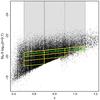 |
Fig. 1 Luminosity selection as a function of redshift. The black dots show the W1 and W4 VIPERS galaxies (with spectroscopic redshift flag between 2 and 9.5). Yellow lines represent the principal magnitude cuts applied in every redshift bin. The green line represents the cut M0 = −19.7 − z made to compare our results to those of K11. |
For the scope of our analysis, the main advantages of VIPERS are the relatively dense sampling of tracers, which allows us to probe density fluctuations down to scales comparable to those affected by galaxy evolution processes, and the large volume that, as discussed in the previous section, allows us to reduce the impact of cosmic variance considerably with respect to previous estimates of galaxy bias at z ~ 1.
The parent PDR-1 VIPERS sample contains 45871 galaxies with reliable redshift measurements. Here we restrict our analysis in the redshift range z = [0.5,1.1] since the number density of objects at larger distances is too small to permit a robust estimate of galaxy bias. To investigate the possible dependence of galaxy bias on luminosity and redshift, we partitioned the catalogue into subsamples by applying a series of cuts in both magnitude and redshift.
The complete list of subsamples considered in this work is presented in Table 1. We considered three redshift bins (z = [0.5,0.7] , [0.7,0.9] , [0.9,1.1]) and applied different luminosity cuts that we obtained by compromising between the need of maximising both completeness and number of objects. Different luminosity cuts within each redshift bin allow us to study the luminosity dependence of galaxy bias at different redshifts. The magnitude cuts, MB = −19.5 − z − 5log (h) and −19.9 − z − 5log (h), that run across the whole redshift range are used to investigate a possible evolution of galaxy bias. In Table 1 the subsamples are listed in groups. The first three groups indicate subsamples in the three redshift bins. The last group indicates subsamples that are designed to match the luminosity cuts performed by K11 (MB = −20.5 − z − 5log (h = 0.7) = −19.72 − z − 5log (h)) and by M05 (MB = −20.0 − 5log (h). The most conservative cut MB = −19.5 − z − 5log (h) guarantees 90% completeness out to z = 1 for the whole galaxy sample and higher for late type objects (see Fig. 1).
Since the analysis presented in this work is based on cell count statistics, a useful figure of merit is represented by the number of independent spheres that can be accommodated within the volume of the survey. Considering intermediate cells with a radius of 6 h-1 Mpc , the number of such independent cells is N = 3869, 5527, 6964 in the three redshift intervals z = [0.5,0.7] , [0.7,0.9] , [0.9,1.1], respectively.
2.2. Mock datasets
We considered a suite of mock galaxy catalogues mimicking the real PDR-1 VIPERS catalogue to assess our ability to measure the mean biasing function and evaluate random and systematic errors.
We used two different types of mock galaxy catalogues. We based the bulk of our error analysis on the first mock galaxy catalogue, which is described in detail in de la Torre et al. (2013). In this set of mocks, synthetic galaxies are obtained by applying the HOD technique to the dark matter halos extracted from the MultiDark N-body simulation (Prada et al. 2012) of a flat ΛCDM universe with (Ωm, ΩΛ, Ωb, h, n, σ8)= (0.27; 0.73; 0.0469; 0.7; 0.95; 0.82). Since the resolution of the parent simulation was too poor to simulate galaxies in the magnitude range sampled by VIPERS, de la Torre & Peacock (2013) applied an original technique to resample the halo field to generate sub-resolution halos down to a mass of M = 1010h-1M⊙. These halos were HOD populated with mock galaxies by tuning the free parameters to match the spatial 2-point correlation function of VIPERS galaxies (de la Torre et al. 2013). Once populated with HOD galaxies, the various outputs were rearranged to obtain 26 and 31 independent light cones mimicking the W1 and W4 fields of VIPERS and their geometry, respectively. In our analysis we considered 26 W1+W4 mock samples. They constitute our set of Parent mock catalogues, as opposed to the Realistic mock catalogues that we obtain from the Parent set by applying the various selection effects (VIPERS footprint mask besides TSR, SSR, and CSR) and by adding Gaussian errors to the redshifts to mimic the random error in the measured spectroscopic redshifts. The mock catalogues were built assuming a constant SSR whereas, as we pointed out, this is a declining function of the apparent magnitude. However, the dependence is weak and only affects faint objects, i.e. preferentially objects at large redshifts. For this reason we decided to explicitly include this dependence by selectively removing objects, starting from the faintest and moving towards brighter objects until we match the observed SSR(m) (Guzzo et al. 2014).
The average galaxy number densities in the mocks are listed in Col. 4 of Table 1. For z ≤ 0.9 the number density in the mocks is similar or somewhat smaller than in the real catalogue. This discrepancy increases with the luminosity and probably originates from the uncertainty in the procedure to HOD-populate halos with bright mock galaxies. The consequence for our analysis is an overestimation of the random errors in the measurement of the bias of VIPERS galaxies. At higher redshift the trend is reversed; the number density of objects in the mocks is systematically larger than in the real catalogue. In this case, to avoid underestimating errors, we randomly diluted the galaxies in the mocks. Hence the perfect match of number densities in the redshift bin z = [0.9,1.1], as shown in the table.
VIPERS subsamples.
On the smallest scale investigated in this paper, R = 4h-1 Mpc , the second-order statistics of simulated galaxies and the variance of the galaxy density field are underestimated by ~10% (Bel et al. 2014). Therefore, to check the robustness of our bias estimate to the galaxy model used to generate the mock catalogues and to the underlying cosmological model, we considered a second set of mocks. These were obtained from the Millennium N-body simulation (Springel et al. 2005) of a flat ΛCDM universe with (Ωm, ΩΛ, Ωb, h, n, σ8) = (0.25; 0.75; 0.045; 0.73; 1.00; 0.9) and using the semi-analytic technique of De Lucia & Blaizot (2007), an alternative to the HOD. As a result of the limited size of the computational box, it was possible to create light cones with an angular size of 7 × 1 deg2, i.e. smaller than the individual W1 and W4 fields. Overall, we considered 26 + 26 reduced versions of the W1+W4 fields. From these light cones we created a corresponding number of Realistic mock catalogues.
Robustness tests that involve both types of mock catalogues were restricted to a limited number of samples (one for each redshift bin). In these tests we simply compared the errors in the bias estimates after accounting for the larger cosmic variance in the Millennium mocks. Since these robustness tests turned out to be successful in the sense that errors estimated with the two sets of mocks turned out to be consistent with each other, we do not mention these mocks again and, for the rest of the paper, fully rely on the error estimates obtained from the HOD mocks.
3. Theoretical background
In this section we briefly describe the formalism proposed by Dekel & Lahav (1999) and the method that we use to estimate bias from galaxy counts. The key step is the procedure to estimate the galaxy PDF, P(δg), from the measured probability of galaxy counts in cells, P(Ng). We review some of the techniques proposed to perform this crucial step and describe in detail the technique used in this work.
3.1. Stochastic non-linear bias
Dekel & Lahav (1999) proposed a probabilistic approach to galaxy bias in which non-linearity and stochasticity are treated independently. In this framework, galaxy bias is described by the conditional probability of galaxy over-density, δg, given the mass over-density δ: P(δg | δ). Both quantities are smoothed on the same scale and treated as random fields. If biasing is a local process then P(δg | δ) fully characterises galaxy bias. Key quantities formed from the conditional probability are the mean biasing function 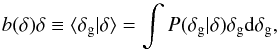 (1)and its non-trivial second-order moments
 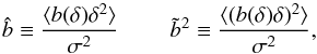 (2)where σ2 ≡ ⟨δ2⟩ is the variance of the mass over-density field on the scale of smoothing. The quantity
  represents the slope of the linear regression of δg against δ and is the natural generalisation of the linear bias parameter. The ratio
  quantifies the deviation of the mean biasing function from a straight line. It measures the non-linearity of the mean biasing relation and, in realistic cases, is close to unity. In the limit of linear and deterministic bias, the two moments and
  coincide with the (constant) mean biasing function b(δ) = bLIN, where bLIN is the familiar linear bias parameter. We note that
  is sensitive to the mass variance and scales as
  . On the contrary, the moments’ ratio is very insensitive to it,
  (Sigad et al. 2000). These scaling relations are used in Sect. 5 to compare results obtained assuming different values of σ8. There are other useful parameters related to galaxy bias that can be measured from the data. One is the ratio of variances bvar ≡ (σg/σ)2 in which σg is measured from counts in cells and σ depends on the assumed cosmological model. Another quantity is the inverse regression of δ over δg,
  that requires an estimate of the galaxy and the mass density fields (Sigad et al. 1998). In the case of non-linear deterministic bias these quantities differ from
  . Specifically, if the non-linearity parameter is larger (smaller) than unity then they are biased high (low) with respect to (Dekel & Lahav 1999).
In this paper we focus on the parameter, a choice that allows us to compare our results with those of K11 (but not with M05, in which the focus is instead on  ). Fortunately, as we shall see, the small degree of non-linearity makes these two choices almost equivalent.
If bias is deterministic, then it is fully characterised by the mean biasing function b(δ)δ. However, we do not expect this to be the case since galaxy formation and evolution are regulated by complex physical processes that are not solely determined by the local mass density. Therefore, for a given value of δ there is a whole distribution of δg about the mean b(δ)δ. This scatter, often referred to as bias stochasticity, is contributed by two sources: shot noise due to the discrete sampling of a continuous underlying density field and those astrophysical processes relevant to the formation and evolution of galaxies that do not depend (solely) on the local mass density.
Previous studies (Branchini 2001; Marinoni et al. 2005; Viel et al. 2005; Kovač et al. 2011) that, like this one, used the galaxy 1-point PDF to recover the biasing function ignored the impact of stochasticity and assumed a deterministic bias. We aim to improve the accuracy of the bias estimator by taking bias stochasticity into account and we do this by assuming that shot noise is the only source of stochasticity. This simplifying assumption can be justified theoretically by both numerical and analytic arguments. Numerical experiments in which semi-analytic galaxies are used to probe the mass density field in samples mimicking SDSS (Szapudi & Pan 2004, see Figs. 11 and 16) and 2MRS (Nusser et al. 2014, see Fig. 1), i.e. two surveys with galaxy number densities similar to that of VIPERS, do indeed show that shot noise is the dominant source of scatter. More specifically, Poisson noise accounts for the scatter in the δg versus δ relation except at large over-density where the relation is over-dispersed. Analytic arguments in the framework of the halo model also confirm that the main source of stochasticity is shot noise with the halo-halo scatter providing a significant contribution for faint objects alone (Cacciato et al. 2012). Assessing the impact of this shot noise only assumption is not simple, but some arguments can be made to quantify the systematic effect of underestimating stochasticity.
An upper limit can be obtained when stochasticity is ignored altogether. In the case of linear and stochastic bias, for example, and would be equal whereas binv would be systematically larger by about 10% (Somerville et al. 2000). The more realistic case of a non-linear and stochastic bias was considered by Sigad et al. (2000) using numerical simulations again. In this case, the effect of ignoring stochasticity is that of overestimating both and . The amplitude of the effect depends on both the cosmological model assumed and the scale considered. To obtain estimates relevant to our analysis we repeated the Sigad et al. (2000) test in Sect. 4.1. The results, which we anticipate here, indicate that and are overestimated by 8(4)% on a scale of 4(8) h-1 Mpc . As for the ratio,  we also confirm that it is remarkably insensitive to stochasticity and, as expected, to the model adopted (Sigad et al. 2000).
Analyses of the datasets may also constrain the size of the effect. Galaxy clustering, higher order statistics, or gravitational lensing generally indicate that galaxy bias cannot be linear and deterministic. However, as we anticipated in the introduction, it is not possible to disentangle the effects induced by non-linearity and stochasticity, except for the case of relative bias between two types of tracers. With respect to this, the largest stochasticity  so far was measured by Wild et al. (2005). If ignored, this would induce a systematic error of ~20% on the relative moments.
Overall, the variety of evidence indicates that if stochasticity is ignored then σb and are overestimated by 10−20%, whereas their ratio is unaffected. However, we stress that in our work stochasticity is, at least in large part, taken into account. Therefore, we expect that our assumption that shot noise is the only source of bias stochasticity generates systematic errors well below the 10% level.
3.2. Direct estimate of b(δ)δ
Under the hypothesis that bias is deterministic and monotonic the mean biasing function, b(δ)δ, can be estimated by comparing the PDFs of the mass and of the galaxy over-density. We let C(δ) ≡ P( >δ) and Cg(δg) ≡ P( >δg) be the cumulative probability distribution functions [CDFs] obtained by integrating the two PDFs. Monotonicity guarantees that the ranking of the fluctuations δ and δg is preserved and b(δ)δ can be obtained by equating the two CDFs at the same percentile, 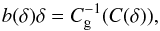 (3)where
  indicates the inverse function of Cg.
Equation (3) provides a practical recipe to estimate galaxy bias from observed counts in cells of a given size. It requires three ingredients: the galaxy over-density δg, its PDF, and that of δ. δg can be estimated from galaxy counts in cell, Ng as  (4)where ⟨Ng⟩ represents mean over all counts. From Eq. (4) one can form the galaxy PDF, P(δg) and the count probability P(Ng). The biasing function can then be obtained by comparing Cg(δg) with a model C(δ).
This simple bias estimator has been used by several authors (Sigad et al. 2000; Branchini 2001; Marinoni et al. 2005; Viel et al. 2005; Kovač et al. 2011). It is potentially affected by several error sources that should be systematically investigated. The first error source is shot noise that affects the estimate of δg from Ng. Shot noise induces stochasticity in the bias relation in contrast with the hypothesis of deterministic bias. Stochasticity affects the estimate of b(δ)δ from Eq. (3), especially at large values of δg, where the CDF flattens and the evaluation of the inverse function becomes noisy. A second issue is the mass PDF for which no simple theoretical model is available. The last error source is redshift distortions. Galaxy over-densities are computed using the redshift of the objects rather than distances. This induces systematic differences between densities evaluated in real and redshift space (Kaiser 1987).
All these issues potentially affect the estimate of galaxy bias and should be properly quantified and accounted for. In the next section, we review some existing estimators designed to minimise the impact of the shot noise and propose a new estimator that we apply in this paper. We investigate the performance of this new strategy in Sect. 4.
3.3. From P(Ng) to P(δg)...
The probability of galaxy counts, P(Ng), can be expressed as 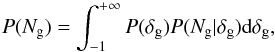 (5)where the conditional probability function P(Ng | δg) specifies the way in which discrete galaxies sample the underlying, continuous field. The common assumption that galaxies are a local Poisson process implies that
 ![Mathematical equation: \begin{equation} P(N_{\rm g} | \delta_{\rm g})=\frac{\left[\langle N_{\rm g}\rangle (1+\delta_{\rm g})\right]^{N_{\rm g}} {\rm e}^{-\langle N_{\rm g} \rangle(1+\delta_{\rm g})}}{N_{\rm g}!} \cdot \label{eq:kernel} \end{equation}](/articles/aa/full_html/2016/10/aa24448-14/aa24448-14-eq119.png) (6)\pagebreak
(6)\pagebreak
The Poisson model provides a good match to numerical experiments except at large densities where a negative binomial distribution seems to provide a better fit (Sheth 1995; Somerville et al. 2001; Casas-Miranda et al. 2002). In this work we adopt the Poisson model. However, different forms for P(Ng | δg) could be considered as well.
The following strategies have been proposed to estimate P(δg) from P(Ng) using Eq. (5):
-
Richardson-Lucy deconvolution. Szapudi & Pan (2004) proposed this iterative, non-parametric method to reconstruct P(δg) by comparing the observed P(Ng) to that computed from Eq. (5) at each step of the iteration, starting from an initial guess for P(δg).
-
Skewed lognormal model fit. This parametric method was also implemented by Szapudi & Pan (2004). In this approach one assumes a skewed lognormal form for P(δg) and then determines the four free parameters of the model by minimising the difference between Eq. (5) and the observed P(Ng).
-
Gamma expansion [ΓE]. Among the various forms proposed to model the galaxy PDF, the Gamma expansion, defined by expanding the Gamma distribution on a basis of Laguerre polynomials (Mustapha & Dimitrakopoulos 2010) captures the essential features of the galaxy density field. The expansion coefficients directly depend on the moments of the observed counts. Because of this, the full shape of the galaxy PDF can be recovered directly from the observed P(Ng) with no need to integrate Eq. (5).
Szapudi & Pan (2004) have tested the ability of the first two methods in reconstructing the PDF of halos and mock galaxies obtained from N-body simulations. They showed that a successful reconstruction can be obtained when the sampling is ⟨Ng⟩ ≥ 0.1; safely a factor 3 smaller than the smallest mean galaxy density in our VIPERS subsamples. Bel et al. (2016) extensively tested the ΓE-method and showed, using the same mock catalogues as in this paper, that this method reconstructs the PDF of a VIPERS-like galaxy distribution with an accuracy that is superior to that of the other methods. This comes at the price of discarding counts in cells that overlap the observed areas by less than 60%, which is a constraint that further reduces deviations from the Poisson sampling hypothesis.
To illustrate the performance of the ΓE-method we plot, in Fig. 2, the galaxy PDFs ΓE-reconstructed from the 26 Realistic mock VIPERS subsamples with galaxies brighter than MB = −19.1 − z − 5log (h) in the range z = [0.7,0.9]. The blue dashed curve represents the mean among the mocks and the blue band the 1σ scatter. The scatter for cells of R = 8h-1 Mpc is larger than for R = 4h-1 Mpc and is driven by the limited number of independent cells rather than sparse sampling.
The reconstruction is compared with the “reference” PDF (solid, red line) obtained by averaging over the PDFs reconstructed, with the same ΓE method, from the Parent mock catalogues. We regard this as the “reference” PDF since, as shown by Szapudi & Pan (2004) and checked by us, when the sampling is dense, all the above reconstruction methods recover the PDF of the mass, P(Ng) and the mean biasing function very accurately. In the plot we show P(1 + δg)(1 + δg) to highlight the low- and high-density tails, where the reconstruction is more challenging. The reconstructed PDF underestimates the reference PDF in the low- and high-density tails and overestimates it at δ ~ 0. Systematic deviations in the low- and high-density tails are to be expected since the probability of finding halos, and therefore mock galaxies, in these regimes significantly deviates from the probability expected for a Poisson distribution. However, these differences are well within the 1σ uncertainty strip as shown in the bottom panels of each plot.
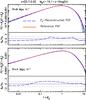 |
Fig. 2 Reconstructed PDF of the mock VIPERS galaxies measured in cells of R = 4h-1 Mpc (top) and R = 8h-1 Mpc (bottom). The blue solid curve represents the reference galaxy PDF obtained by averaging over the PDFs reconstructed from the Parent mocks using the ΓE method. The blue dashed curve shows the average PDF reconstructed from the Realistic mocks using the same method. The blue shaded region represents the 1σ scatter among the 26 Realistic mocks. We plot P(1 + δg)(1 + δg) to highlight the performance of the reconstruction at high and low over-densities. We note the different Y-ranges in the two panels. The bottom panels in each plot show the difference Δp between the reconstructed and reference PDFs in units of the random error σp. Horizontal, dashed lines indicate systematic errors equal to 1σp random uncertainties. |
The ΓE method used to reconstruct the galaxy PDF from discrete counts is implemented as follows:
-
We consider as the input dataset one of the volume-limited, luminosity complete subsamples listed in Table 1. The position of each object in the catalogue is specified in redshift space, i.e. by its angular position and measured spectroscopic redshift.
-
Spherical cells are thrown at random positions within the surveyed region. We consider cells with radii R = 4, 6, and 8 h-1 Mpc . The smallest radius is set to guarantee ⟨Ng⟩ ≥ 0.3. The largest radius is set to have enough cell statistics to sample P(Ng) at large Ng. We only consider cells that overlap by more than 60% with the observed areas. This constraint reduces deviations from Poisson statistics (Bel & Marinoni 2014). Counts in the partially overlapping cells are weighted by the fraction f of the surveyed volume in the cell: Ng/f. The probability function P(Ng) is then computed from the counts frequency distribution.
-
We use the measured P(Ng) and its moments to model the galaxy PDF with the ΓE method that we compute using all factorial moments up to the sixth order.
3.4. ....and from P(δg) to b(δ)δ.
To estimate the mean biasing function from the galaxy PDF, we solve Eq. (3). To do so, we assume that shot noise is the main source of stochasticity and that a reliable model for the mass PDF is available. Despite its conceptual simplicity, this procedure requires several non-trivial steps that we describe below. The uncertainties introduced in each step are estimated in the next section. The procedure is as follows:
-
We start from the galaxy PDF estimated from the measured P(Ng), as described in the previous section.
-
We assume a model PDF for the mass density field in redshift space. Rather than adopting some approximated, analytic model, we measure the mass PDF directly from a dark matter only N-body simulation with the same characteristics and cosmological model as the Millennium run (Springel et al. 2005), that is not based on the same model used to build the HOD-mock VIPERS catalogues. The use of an incorrect mass PDF is yet another possible source of systematic errors that we quantify in Sect. 4. However, this error is expected to be small since
and are mainly sensitive to σ and their ratio is largely independent of the underlying cosmology (Sigad et al. 2000). -
After computing the cumulative distribution function from the mass and galaxy PDFs, we use Eq. (3) to estimate the mean biasing function.
-
We determine the maximum over-density δMAX at which the reconstructed mean biasing function can be considered reliable. To estimate δMAX we compare the measured P(Ng) with the estimated P(Ng) following the procedure described in Sect. 4.4.4.
-
We estimate the second-order moments
and and their ratio by integrating over all δ up to δMAX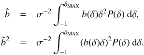 (7)and test the robustness of the result with respect to the choice of δMAX.
4. Error sources
In this section we review all possible sources of uncertainty that might affect the recovery of the biasing function and assess their amplitude using mock catalogues. In this process we need to consider a reference biasing function to compare with the results of the reconstruction. This could be estimated directly from the distribution of the dark matter particles and mock galaxies within the simulation box. However, we use the mean biasing function obtained from the Parent mocks as reference. We justify this choice as follows. First, Szapudi & Pan (2004) showed that when the sampling is dense both the Richardson-Lucy and the skewed lognormal fit methods recover the mean biasing function with high accuracy. Second, in Sect. 3.3 we found that when the sampling is dense the ΓE method accurately recovers the mean biasing function in the Parent mocks.
4.1. Sensitivity to the galaxy PDF reconstruction method
Most of the previous estimates of the mean biasing function did not attempt to account for shot noise directly. This choice can hamper the recovery of b(δ)δ when the sampling is sparse. To estimate errors induced by ignoring shot noise and quantify the benefit of using the ΓE method we compared the biasing functions reconstructed using both procedures. The result of this test is shown in Fig. 3. The red curve represents the reference biasing function obtained by averaging over the Parent mocks. In each mock the biasing function was estimated from the galaxy PDF using the ΓE method. The blue dashed curve represents the same quantity estimated from the 26 Realistic mocks using the ΓE method. The blue band represents the 2σ scatter. For negative values of δg the reconstructed biasing function is below the reference biasing function, but the trend is reversed for δg> 0, reflecting the mismatch between the reconstructed and reference PDFs in Fig. 2. The discrepancy however, is mostly within the 2σ scatter (horizontal dashed line in the bottom sub-panels). On the contrary, the biasing function obtained from the “direct” estimate of δg (brown dot-dashed curve and the corresponding 2σ scatter, orange band) is significantly different from the reference function. The discrepancy increases at low densities and for small spheres, i.e. when the counts per cell decrease and the shot noise is large.
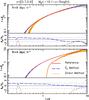 |
Fig. 3 Mean biasing function of mock VIPERS galaxies computed from counts in cells of R = 4h-1 Mpc (bottom panel) and R = 8h-1 Mpc (top panel). The magnitude cut and redshift range of the mock VIPERS subsample, indicated in the plot, are the same as Fig. 2. Solid red curve: reference biasing function obtained from the Parent mock catalogues. Blue dashed curve and blue-shaded region: average value and 2σ scatter of the biasing function reconstructed from the Realistic mocks using the ΓE method. Brown dot-dashed curve and orange-shaded band: average value and 2σ scatter of the biasing function reconstructed from the Realistic mocks using a “direct” estimate of the galaxy PDF. Bottom sub-panels: difference Δp between the reconstructed and reference PDFs in units of the random error σp. Dashed lines indicate systematic errors equal to 1σp random errors. |
4.2. Sensitivity to the mass PDF
Another key ingredient of the mass reconstruction is the mass PDF. In principle this quantity could be obtained from galaxy peculiar velocities or gravitational lensing. However, in practice, errors are large and would need to be averaged out over scales much larger than the size of the cells considered here. For this reason we need to rely on theoretical modelling. Coles & Jones (1991) and Kofman et al. (1994) found that the mass PDF can be approximated by a lognormal distribution and this model was indeed adopted in previous reconstructions of the biasing function (e.g. M05; Wild et al. 2005; K11).
However, the lognormal approximation is known to perform poorly in the high- and low-density tails and for certain spectra of density fluctuations. An improvement over the lognormal model is represented by the skewed lognormal distribution (Colombi 1994). This model proved to be an excellent approximation to the PDF of the dark matter measured from N-body experiments over a wide range of scales and of over-densities (Ueda & Yokoyama 1996). The impact of adopting either model for the mass PDF can be appreciated in Fig. 4. The solid red curves represent the same biasing functions shown in Fig. 3 obtained from the galaxy PDFs of the Parent mocks and from a mass PDF obtained directly from an N-body simulation with the same cosmological parameter and size as the Millennium simulation using the output corresponding to z = 0.8. As in the previous test, we consider the red solid curve as the reference biasing function. The brown dot-dashed curve shows the mean biasing function reconstructed assuming a lognormal model for the mass PDF, i.e. a lognormal fit to the PDF measured from the N-body simulation. The curve represents the average among 26 mocks and the orange band is the 2σ scatter. For R = 8h-1 Mpc , the biasing function is systematically below the reference whereas for R = 4h-1 Mpc is above the reference at both high and low densities. The mismatch is very large and significantly exceeds the 1σ scatter (bottom sub-panels). The skewed lognormal model (blue dashed curve) performs significantly better with differences well below 1σ except at very negative δ values.
We conclude that, for the practical purpose of reconstructing galaxy bias, the mass PDF measured from N-body data and a skewed lognormal fit perform equally well. The main advantage of using the latter would be the possibility of determining the four parameters of the fit experimentally. Since, however, the parameters are poorly constrained by observations, we decided to adopt the mass PDFs from N-body simulations. This choice introduces a dependence on the cosmological model, however, that is mostly captured by one single parameter, σ, for which and exhibit a linear dependent. With respect to this, the mass PDF used to obtain the biasing functions in Fig. 4 is not the true mass PDF since it is obtained from an N-body simulation that uses a cosmological model that is different from the model used to produce the mock catalogues. We did this on purpose to mimic the case of the real analysis for which the underlying cosmological model is not known.
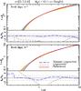 |
Fig. 4 Solid red curve: reference mean biasing function of Fig. 3 computed using the mass PDF from N-body simulations. Brown dot-dashed curve and orange band: biasing function obtained using a lognormal fit to the mass PDF and 2σ scatter from the mocks. Blue dashed curve and blue band: biasing function obtained using a skewed lognormal fit to the mass PDF and 2σ scatter from the mocks. Bottom panels: difference Δp between the reconstructed and reference PDFs in units of the random error σp. Dashed lines indicate systematic errors equals to 1σp random errors. |
4.3. Sensitivity to redshift distortions
Galaxy positions are measured in redshift space, i.e. using the observed redshift to estimate the distance of the objects. The presence of peculiar velocities induces apparent radial anisotropies in the spatial distribution of galaxies and, as a consequence, modifies the local density estimate and their PDF (Kaiser 1987). However, our goal is to reconstruct the mean biasing function in real space without redshift distortions. Considering the difficulties and uncertainties in determining the galaxy PDF in real space, one could instead consider the galaxy and mass PDFs both measured in redshift space under the assumption that peculiar velocities induce similar distortions in the spatial distribution of both dark matter and galaxies so that they cancel out when estimating the mean biasing relation from Eq. (3). In the limit of the Gaussian field, linear perturbation theory and no velocity bias, the cancelation is exact. However, non-linear effects have a different impact on the mass and galaxy density fields and induce different distortions in their respective PDFs. To assess the impact of these effects we compared the mean biasing function of mock galaxies reconstructed from PDFs estimated in real and redshift space.
The results are shown in Fig. 5. The solid red curve represents the mean biasing function of galaxies in the Realistic mock catalogues estimated using the PDFs of galaxies and mass in real space. The blue dashed line shows the same function estimated in redshift space. Both curves are obtained by averaging over the 26 mocks and the blue band represents the 2σ scatter in redshift space. The redshift space biasing function underestimates the true biasing function in low-density regions and overestimates it at high densities, i.e. in the presence of highly non-linear flows. The difference is systematic but its amplitude is within the 2σ random errors estimated by adding in quadrature the scatter among mocks in real and redshift space (bottom panels in each plot). The biasing functions shown in Fig. 5 represents a demanding test in which we consider the smallest cells of 4 h-1 Mpc where deviations from linear motions are larger. The discrepancy decreases if the size of the cell increases.
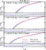 |
Fig. 5 Mean biasing function estimated in real space (solid, red curve) and redshift space (dashed blue curve and its 2σ uncertainty band). Counts are performed in spherical cells with a radius of 4 h-1 Mpc . The luminosity cut and the redshift range is indicated in each panel. The width of each band represents the scatter among mocks. In the bottom part of each plot we show the difference Δp between the reconstructed and reference PDFs in units of σTOT, where σTOT accounts for the rms scatter in both the real- and redshift-space mocks. Dashed lines indicate where systematic errors equal to 1σTOT random errors. |
These systematic differences induce errors in the estimated moments and . To quantify the effect we computed the moments as a function of δ (i.e. by varying δMAX in Eq. (7)) both in real and redshift space. The results are shown in Fig. 6. The plots show the per cent difference between the moments measured in redshift versus real space. The panels and curves refer to the same redshift bins and magnitude cuts as in Fig. 5. Systematic errors induced by redshift distortions are ~2% for and for (not shown) and one order of magnitude smaller for . They provide the main contribution to the total systematic errors listed in Table 2 and are of the same size, although somewhat smaller than the random errors.
Considering the absolute and relative size of these errors, we perform our analysis in redshift space.
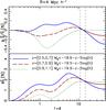 |
Fig. 6 Bottom panel: per cent difference between the |
4.4. Error estimate
Different sources of errors affect the recovery of the biasing function. One error source is cosmic variance due to the finite volume of the sample. This source dominates the error budget of the M05 and K11 analyses.
The other sources are the shot noise induced by discrete sampling and the limited number of independent cells used to build the probability of galaxy counts P(Ng). In the VIPERS survey, which is based on a single-pass strategy, sparse sampling is more of an issue than in the M05 and K11 cases. The cumulative effect of the single pass strategy and colour preselection reduces the sampling rate to ~35% on average with significant variations across quadrants. The survey geometry, characterised by gaps and missing quadrants that occupy ~25% of the would-be continuous field, further dilutes the sampling (we consider cells that overlap up to 40% with unobserved regions) and limits the number of independent cells that can be accommodated within the survey. Our PDF reconstruction strategy is designed to minimise these effects that, nevertheless, induce random and systematic errors that need to be estimated. We do this with the help of both the Parent and Realistic mock catalogues. The former provide the reference mean biasing function. Errors are estimated by comparing the bias function reconstructed from the Realistic mocks to the reference mocks. The procedure is detailed below and the estimated errors are listed in Table 2.
Bias parameters of VIPERS galaxies and their errors.
4.4.1. Total random error
To estimate the total random error σRND, we proceed as follows. We reconstruct the mean biasing function in each of the Realistic mock catalogues, compute the average over the 26 mocks and, finally, estimate the scatter around the mean. The rms scatter provides an estimate of the total random error. All sources of uncertainties contribute to this error (e.g. cosmic variance, shot noise, and limited number of cells), which may affect the recovery of the biasing function. Total random errors for and are listed in Cols. 6 and 10 of Table 2, respectively.
4.4.2. Cosmic variance
To assess the contribution of the cosmic variance, σCV, to the error budget, we proceed as for the estimate of total random errors using, however, the Parent catalogues rather than the Realistic catalogues. Since errors in the bias reconstruction are mainly driven by discrete sampling and in the Parent catalogues the sampling is dense, the rms scatter among these mocks is dominated by cosmic variance. Cosmic variance contributions to errors in and are shown in Cols. 7 and 11 of Table 2, respectively. It turns out that the contribution of the cosmic variance is of the same order as that of the sparse sampling and, unlike in the case of M05 and K11, it does not dominate the error budgets.
4.4.3. Systematic errors
Following K11, we compute systematic errors, σSYS, as the average offset of the bias estimates in the Realistic and the Parent catalogues, i.e. σSYS = ⟨XRealistic − XParent⟩, where X is either or and the mean is over the 26 pairs of mocks. These systematic errors are plotted in the bottom panels of Fig. 3 (blue, dashed curves). Their amplitudes at δMAX are listed in Cols. 8 and 12 of Table 2. These systematic errors are of the same order as the random errors and as the errors induced by redshift distortions discussed in Sect. 4.3. These systematic errors include those induced by redshift distortions. The fact that they are of the same order as those discussed in Sect. 4.3 indicates that they dominate the budget of systematic errors.
Our systematic errors are similar to those estimated by K11 (upper part of their Table 2) from the zCOSMOS sample, which is significantly small than VIPERS. As these errors do not seem to depend on the volume of the survey, we conclude that they can be regarded as genuinely systematic. Systematic errors on are on average positive, meaning that the mean slope of the reconstructed biasing function typically overestimates the true biasing function. For the non-linear bias, parameter systematic errors are preferentially negative, indicating that the reconstruction procedure has the tendency to underestimate the non-linearity of the biasing function.
4.4.4. The value of δMAX
Our bias estimator becomes progressively less reliable as the density increases, for two reasons: first, the numerical solution to Eq. (3) becomes unstable when the cumulative distribution functions approach unity, i.e. in correspondence of the high peaks of the mass and galaxy density fields. In this regime, small errors in the estimated galaxy PDF propagate into large uncertainties in δ; second, as anticipated in the previous section, the scatter in the δg versus δ relation is larger than Poisson. Our assumption that Eq. (6) is valid at all δ leads to underestimating the high-density tail of the galaxy PDF and, consequently, the value of .
Our mock catalogues can be used to estimate the first type of error, but cannot fully account for the second type of error since our mock galaxies are sampled from dark matter halos assuming Poisson statistics. We therefore take the alternative route of reducing the impact of deviations from Poisson statistics at high densities. We do this by setting a sensible maximum over density value, δMAX, at which we compute the bias moments. The value of this threshold is computed as follows:
-
1.
We consider the difference ΔP between the “true” Pt(Ng) measured in theRealistic mock catalogues and the reconstructed Pr(Ng) estimatedthrough Eq. (5).
-
2.
We search for the first Ng value, N1, at which ΔP> 2σP, where σP is the rms scatter in the mocks.
-
3.
We search for the first Ng value, N2, at which | ΔP/Pt(Ng) | > 0.5.
-
4.
We take NMAX = Min [N1,N2] and compute the corresponding over-density in galaxy counts δg,MAX = NMAX/ ⟨N⟩.
-
5.
We obtain the corresponding mass over-density δMAX from δg,MAX from the estimated mean biasing function.
The largest over-density at which we search for a solution to Eq. (3) is δMAX, and this is also the over-density at which we estimate the bias moments. This value is clearly model dependent since it was estimated from the VIPERS mocks. An alternative way of setting this threshold would be to look for wiggles in the mean biasing function measured from real data, i.e. spurious features induced by instabilities in the reconstruction procedure. We found that this second criterion is less stringent as it produces δMAX values larger than using mocks. We decided to adopt a conservative approach and use the δMAX thresholds estimated with the first procedure.
With this criterion we obtain different δMAX for the different galaxy subsamples considered in our analysis. This limits our ability to compare results. Since the value of δMAX mainly depends on the radius of the cell, we use one single value for δMAX for a given cell size, irrespective of the other parameters used to define the subsample. These values, which are listed in Table 2, correspond to the minimum δMAX among those computed for all subsamples.
All bias parameters presented in our work were computed at these over-density values. To check the robustness of our results to δMAX we also considered a second, less stringent threshold obtained by taking the maximum value of δMAX among those of the various subsamples for a given cell size. This second set of δMAX that we denote as  , is also listed in Table 2 together with the corresponding estimates for the bias moments (values in parenthesis).
5. Results
In this section we present the results of our analysis, focusing on the dependence of the mean biasing function and its moments on various quantities. In Sects. 5.1 and 5.2 we explore the bias dependence on magnitude and redshifts, respectively. In both cases we fix the radius of the cells equal to 6 h-1 Mpc . The dependence on the cell size is investigated in Sect. 5.3. Results are summarised in Sect. 5.4 and listed in Table 2.
5.1. Magnitude dependence
The different solid curves in Fig. 7 represent the mean biasing function of VIPERS galaxies reconstructed from counts in cells of radius 6 h-1 Mpc for different magnitude cuts for three different redshift shells (the three panels). We applied a small horizontal offset δ = 0.015 to the curves to avoid overlapping error bars. We plot (1 + δ) in logarithmic units both to ease the comparison with similar plots in the literature and to highlight deviations from linearity in the low-density regions. Error bars represent the 2σ random scatter computed from the Realistic mocks.
The magnitude range that we are able to explore is set by competing constraints: the faint limit reflects the requirement of maximising the completeness of the sample whereas the bright limit is set by requiring ⟨Ng⟩ > 0.3 per cell. As a result, the magnitude range shrinks with the redshift: at z = [0.5,0.7] it spans a range ΔMB = 1.4 whereas at z = [0.9,1.1]ΔMB = 0.5.
In the upper plot the curves corresponding to the different magnitude cuts are well separated for δg< 0. The separation reduces and then disappears with the redshift. This is not surprising since at z ≥ 0.9 the luminosity range is very narrow, as we have seen. No significant trend with luminosity is seen at large over-density. These features, or the lack of them, are robust to variations in the size of the cells in the range R = [4,8]h-1 Mpc (see Table 2) and confirm the results obtained at lower redshifts from galaxy clustering (e.g. Norberg et al. 2002; Zehavi et al. 2005; Pollo et al. 2006; Coil et al. 2008; Skibba et al. 2014; Arnalte-Mur et al. 2014; Marulli et al. 2013), gravitational lensing (e.g. Coupon et al. 2012) and counts in cells (e.g. M05 and K11).
To further investigate galaxy bias in under-dense regions, we zoom into the δ< 0 range in Fig. 8. The curves are the same as in Fig. 7. The black long-dashed line represents the linear biasing function with a slope matching the value estimated at δMAX, which is listed in Table 2. Since only weakly depends on the magnitude cut we only consider one representative case per panel. The local slope of the biasing function is always steeper than the best-fitting linear bias model. The horizontal, short-dashed line shows the δg = −0.9 threshold. The mass over-density at which this line crosses the biasing curves, δTH, increases with the redshift and, to a lesser extent, with the luminosity. This trend, which was noticed by M05 and, with less significance, by K11, has been interpreted as evidence that low-density regions are preferentially populated by low-luminosity galaxies. Also, the quantity δTH has been regarded as the typical mass over-density below which very few galaxies form.
Figure 8 shows that galaxies can be found at mass over-densities well below δTH. This low-density tail, together with the steepness of the biasing function for δ>δTH, shows that the biasing relation in the under-density region significantly deviates from the linear prescription. Non-linearity increases when decreasing the cell size. As we checked, for R = 4 h-1 Mpc the slope of the biasing curves further increases well above δTH. For R = 8 h-1 Mpc , the difference disappears and the two slopes start to match. Still, the bias curves keep featuring a negative δ tail that cannot be matched by linear models.
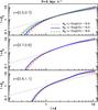 |
Fig. 7 Mean biasing function of VIPERS galaxies from counts in cells of radius 6 h-1 Mpc as a function of the B-band magnitude cut in three redshift ranges indicated in each panel. Curves with different colours and line styles correspond to the different magnitude cuts indicated in upper panel. Error bars with matching colours represent the associated 1σ uncertainty intervals estimated from the mocks. A horizontal offset δ = 0.015 was applied to avoid overlapping error bars. All biasing functions are plotted out to δMAX. |
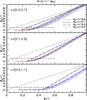 |
Fig. 8 Zoom into the under-density range of Fig. 7. The horizontal short-dashed line represents the over-density threshold δg = −0.9. The long dashed line shows the linear biasing function |

Figure 9 shows the second-order moment (left panels) and the ratio (right panels) of the biasing functions shown in Fig. 7. The same colour-code is used to indicate the magnitude cuts. Large filled symbols refer to measurements performed at δMAX assuming σ8 = 0.9 whereas the slightly offset, smaller open symbols refer to estimates performed at . The values of the corresponding bias moments are listed in Table 2. Error bars represent 1σ total random uncertainties estimated from the Realistic mocks (see Table 2).
In the left panels of Fig. 7, we notice that in the low redshift bin, where the magnitude interval that we probe is larger, increases with the luminosity. This dependence is much weaker for z = [0.7,0.9] and completely absent at higher redshifts. We show results for cells of 6 h-1 Mpc . However, the same trend is also seen for 4 and 8 h-1 Mpc .
The right panels show the non-linear parameter . Values that differ from unity indicate deviations from linear bias (horizontal dashed line). A small but significant degree of non-linearity is present at all redshifts. We do not detect any significant dependence on luminosity in any redshift bin and for any cell size.
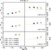 |
Fig. 9 Second-order moments of the mean biasing functions shown in Fig. 7. Left panels: moment |
A common feature of the reconstructed mean biasing functions at z = [0.9,1.1] is the presence of some irregular behaviour (wiggling) at high over-densities. This is the typical fingerprint of an imperfect inversion (Eq. (3)) discussed in Sect. 3.2 and one of the reasons for introducing the threshold δMAX. These irregularities typically arise as a result of sampling rare, large over-densities with a limited number of independent cells. The effect is most evident at large redshifts and for bright magnitude cuts, i.e. when the sampling is sparser. This affects the shape of the reconstructed mean biasing function. However, the impact on the second moments and and, especially, , is rather limited. This is because bias moments are integral quantities (Eq. (7)) weighted by the mass PDF, which peaks at δ ~ 0 and rapidly approaches zero in the high- and low-density tails. Systematic errors in the bias reconstruction at large over-densities are therefore suppressed when computing and and further smoothed out when computing their ratio.
Figure 10 demonstrates the validity of this conjecture. In the left panels we show the values of  computed from Eq. (7). Curves with different line styles refer to the different magnitude cuts indicated in the plot. Error bars with matching colours indicate the 1σ scatter from the mocks. In the interval z = [0.9,1.1] and for the brightest and sparsest sample, flattens for δ> 3, i.e. well below δMAX. Analogous considerations hold for the curve
  shown in the right panels. These trends are robust to the size of the cells.
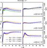 |
Fig. 10 Left: second-order moment |
5.2. Redshift dependence
To explore the bias dependence on the redshift we set a magnitude cut MB = −19.5 − z − 5log (h) and estimated the mean biasing function of brighter galaxies in the three redshift bins. This z-dependent magnitude cut is designed to account for luminosity evolution (Zucca et al. 2009), so that differences in the galaxy bias measured in the different z-bins can be interpreted as the result of a genuine evolution. The results of our analysis are shown in Fig. 11. The plots are analogous to those of Fig. 7 and use the same symbols, colour scheme, and line style. However, we consider cells of different sizes in the three panels.
The biasing function shows little or no evolution in the range z = [0.5,0.9], as demonstrated by the proximity between the dashed-blue (z = [0.5,0.7]) and dot-dashed orange (z = [0.7,0.9]) curves and the overlap of their 1σ error bars. The red solid line, however, is separated fully from the others, indicating that galaxy bias evolves significantly beyond z = 0.9. This evolution is detected both in low- and high-density environments. It implies that δTH increases significantly with the redshift, indicating that evolution shifts galaxy formation towards regions of progressively lower density. At δ> 0 the effect of evolution is that of increasing the slope of the biasing function with z. Since in this range the biasing is close to linear, an estimate of bLIN would reveal a redshift evolution consistent with that observed in several analyses, as detailed in Sect. 6. The same trend is evident in all panels, indicating that the bias evolution is similar in all explored scales.
At high redshifts and for R = 8h-1 Mpc (bottom panel) the biasing function is characterised by some irregularities at moderate values of δ. As pointed out, these have little impact on the estimated values of and . It is reassuring that these anomalies are only seen at high redshifts, confirming the fact that they are induced by poor sampling of the counts probability. All this makes us confident that bias evolution is a genuine feature.
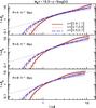 |
Fig. 11 Mean biasing function of VIPERS galaxies with MB< −19.5−z − 5log (h) measured in different redshift bins, characterised by different colours and line-styles, as indicated in the plot. Error bars represents the 1σ scatter in the mocks. The three panels refer to different cell sizes with radii R = 4,6,8h-1 Mpc from top to bottom. A horizontal offset δ = 0.015 was applied to avoid overlapping error bars. All curves are plotted out to δMAX. |
Figure 12 shows the values of and as a function of redshift. The values were obtained by integrating the mean biasing functions in Fig. 11 out to the values δMAX and (large and small symbols, respectively). The corresponding values are listed in Table 2. The colour code is the same as in Fig. 11 and is indicated in the plot. The mean slope of the curve, (left panels), increases significantly beyond z = 0.9 whereas we see little or no evolution at lower redshifts. This shows that the trend seen in Fig. 11 is seen at all scales, indicating that the bias evolution at z> 0.9 is indeed a robust feature. The bias parameter of VIPERS galaxies brighter than MB = −19.9 − z − 5log (h) exhibits a small but significant degree of non-linearity at all redshifts and scales explored in our analysis (right panels); this bias parameter, however, does not significantly evolve with redshift. These results are robust to the luminosity cut since they are also found for galaxies brighter than MB< −19.9 − z − 5log (h).
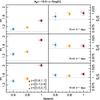 |
Fig. 12 Moments of the mean biasing functions shown in Fig. 11. Panels from top to bottom indicate cells of increasing size. Left panels: |
5.3. Scale dependence
In Fig. 13 we explore the dependence of the bias of VIPERS galaxies on the radius of the cells down to a scale of 4 h-1 Mpc . In the plots we show the mean biasing function of VIPERS galaxies brighter than MB = −19.5 − z − 5log (h) measured at R = 4,6 and 8h-1 Mpc . Different scales are characterised by different colours, as indicated in the plot. The panels show the results in the three redshift shells. At negative over-density the curves are remarkably similar, indicating that δTH and the efficiency of galaxy formation do not depend on the scale in the range [4,8]h-1 Mpc . At δ> 0 the curves steepen with the radius of the cell, indicating that biasing increases with the scale especially at high redshift.
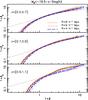 |
Fig. 13 Mean biasing function of VIPERS galaxies with MB< −19.5−z − 5log (h) computed from counts in cells with radii of 4,6, and 8h-1 Mpc . Biasing functions at different scales are indicated with different colours and line styles, as indicated in the plots. Error bars represent the 2σ rms scatter in the mocks. Different panels refer to different redshift shells. An offset δ = 0.015 was applied to avoid overlapping error bars. Curves are plotted out to δMAX. |
A more quantitative assessment of scale dependence is shown in Fig. 14. The value of steadily increases with the cell radius, R, especially at high redshift. This trend may sound counterintuitive; galaxies are expected to trace the mass with increasing accuracy on a larger scale and, consequently, galaxy bias is expected to approach its linear value. This, however, occurs on scales much larger than those considered here (see e.g. Wild et al. 2005). On the scales explored here the halo model predicts that the opposite trend should be observed (see e.g. Fig. 4 of Zehavi et al. 2004). The reason is that in this range of scales the contribution to galaxy clustering of the 1-halo term, which dominates on small scales, is comparable to that of the 2-halo term, which dominates on large scales. The scale of the crossover depends on galaxy type and redshift but it is expected to be bracketed in the range probed by our analysis. This explanation is corroborated by the fact that the values of measured in the HOD mocks, designed following the halo model prescriptions, do show an increasing trend with the size of the cells.
An increase of galaxy bias with the scale was already detected at lower redshifts from the analysis of galaxy clustering (Zehavi et al. 2005) and from weak lensing (Hoekstra et al. 2002; Simon et al. 2007). This is the first detection at relatively high redshift that exploits counts in cell statistics. A small, but significant amount of non-linearity is detected at all redshifts. Unlike , the non-linear parameter seems to be scale independent. These results are robust to magnitude cut since similar trends for and are also seen when one restricts the biasing analysis to objects brighter than MB< −19.9 − z − 5log (h).
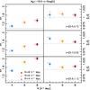 |
Fig. 14 Moments of the mean biasing functions vs. the size of the cell. Panels from top to bottom refer to different redshift ranges indicated in the plot. Left panels: |

5.4. Results from the whole dataset
We now summarise the results presented in this section. Overall, the biasing functions of the VIPERS subsample are in qualitative agreement with those of M05 and K11 with some intriguing differences. At moderate over-densities and out to δMAX, our biasing functions are close to linear with a slope close to  . This is at variance with M05 and K11 whose biasing function flattens at large δ, leading to an anti-bias signature. This feature has been variously interpreted as evidence for quenching processes (Blanton et al. 2000), enhanced galaxy merging rate (Marinoni et al. 2005), and early galaxy formation (Yoshikawa et al. 2001) in high-density regions. We find a similar flattening only if we push our analysis beyond δMAX. However, its statistical significance is less that 2σ. A similar feature was also detected in simulations and interpreted as an artefact due to limitations of the bias estimator at high redshift (Sigad et al. 2000). Given the fact that all these works, including ours, use a similar technique to measure galaxy bias, we suspect that the flattening at large density is not a genuine effect.
At δ< 0 the biasing function significantly deviates from linear prescription and is steeper than . Moreover, the galaxy density remains positive below δTH, indicating that galaxy formation is not entirely quenched even in very low-density environments.
Table 2 lists the bias parameters measured in the VIPERS subsamples of Table 1 together with random and systematic errors estimated from the mocks. We computed all of the parameters by integrating the mean biasing function out to the value δMAX listed in the Table. Altogether the results confirm the various trends that we described in the previous sections: the value of increases with luminosity, scale, and with the redshift beyond z = 0.9. Deviations from linear biasing are small but typically detected with significance larger than 1σ. The non-linear bias parameter is, within the errors, independent of redshift, luminosity, or scale.
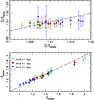 |
Fig. 15 Bottom panel: comparison between |
We obtained errors from the VIPERS mock catalogues designed to match the 2-point statistics of real galaxies but not their abundance or their bias. One consequence of this is that bright galaxies in the subsamples of the mocks are sparser than the real galaxies at z< 0.9 (see Table 1). As a result our random errors somewhat overestimate the real errors. As for the bias, if that of the galaxies in the real sample is different from the mock sample, then our error estimate would be affected. We compared the values of and in the mock and in the real samples to investigate this issue. The resulting scatter plots are shown in Fig. 15. The different points represent the individual subsamples considered in our analysis. Symbols with different colours are used to highlight results obtained with different cell sizes. Error bars represent the rms scatter in the mocks. Most of the points deviates less than 2σ from the expected value (black dashed line), implying that our mocks are realistic and that our errors are indeed reliable.
6. Comparison with previous results
Several authors estimated the bias of galaxies in the same range, z = [0.5,1.1], considered here. The majority of these authors assumed linear bias and estimated the bias parameter from galaxy clustering (Coil et al. 2006, 2008; Meneux et al. 2006, 2008, 2009; Coupon et al. 2012; Marulli et al. 2013; Skibba et al. 2014; Arnalte-Mur et al. 2014). Only a handful of papers addressed the issue of non-linear or scale-dependent bias at these redshifts (M05; K11; Simon et al. 2007; Jullo et al. 2012). In this section, we compare our results with both types of analyses. First we compare our estimated non-linear bias parameter with available measurements from previous studies. Then we consider the most recents estimates of the linear bias parameter bLIN in this redshift range available in the literature and compare them with our value of . In these comparisons all results were rescaled to the value σ8 = 0.9 adopted in this paper whenever required.
6.1. Galaxy bias from counts in cells
In Fig. 16 we plot the values of and obtained from our analysis as a function of redshift (filled and open red dots) and compare these values to those obtained by M05 (green triangles) and K11 (blue squares) from counts in cells following a procedure similar to ours. We do not consider the results of the analyses of Simon et al. (2007) and Jullo et al. (2012) since these authors estimate the so-called correlation parameter that accounts for both non-linearity and stochasticity.
We only considered objects that, at a given redshift, span a similar range of magnitudes to avoid mixing evolution and luminosity dependence. For VIPERS we consider objects with MB< −19.1 − z − 5log (h). For zCOSMOS we consider objects above a similar cut-off, MB = −19.22 − z − 5log (h). For the VVDS-Deep sample, M05 use a redshift-independent luminosity threshold of MB = −20.0 − 5log (h), which is comparable with the above cut-offs in the range z = [0.8,1.1]. We considered an additional VIPERS subsample cut at the same constant magnitude limit as M05 to improve the consistency in the comparison with VVDS.
In the case of M05, the values of and shown in Fig. 16 were inferred from the published values of and  . In addition, M05 do not provide the errors for . The error bars shown in the plot were extrapolated from the errors on under the assumption that the ratio of the errors on and those on are the same for the two datasets. The comparison between zCOSMOS and VIPERS shows that this assumption is approximately valid. The zCOSMOS points are plotted at the centre of their redshift bins. In the VVDS case we added an offset Δz = + 0.02 to avoid overlapping. Finally, we restrict our comparison to counts in cells of R = 8h-1 Mpc since this is the minimum cell size considered by K11 and the only one common to the three analyses.
The values of zCOSMOS galaxies (bottom panel) are in agreement with those of VIPERS galaxies. These values increase with redshift in both cases. This trend is more evident in the zCOSMOS case, while for VIPERS the evolution is detected only with a significance of ~1σ only. Our results do not match those of M05 at z = 0.8, where the two samples overlap. The significance of the discrepancy, however, is about 1σ. A similar mismatch was observed between VVDS-Deep zCOSMOS and interpreted by K11 in terms of different clustering amplitude in the two datasets (McCracken et al. 2007; Meneux et al. 2009; Kovač et al. 2011). Indeed, zCOSMOS is characterised by prominent structures and large spatial coherence as opposed to the VVDS Deep field. This difference was interpreted as a manifestation of cosmic variance. The VIPERS survey was designed to reduce the impact of cosmic variance and solve these types of controversies. In this specific case, the agreement between VIPERS and zCOSMOS galaxies suggests that the bias of the latter is closer to the cosmic mean than that of the VVDS-Deep field.
The comparison among the non-linear bias parameters of the three galaxy samples (upper panel of Fig. 16) corroborates this conclusion. The values of for zCOSMOS and VIPERS galaxies agree with each other and significantly deviates from unity. Thanks to the smaller error bars in VIPERS these deviations are now detected with higher statistical significance. Deviations from non-linear bias in the VVDS-Deep are larger than in VIPERS but the statistical significance for this mismatch is just about 1σ.
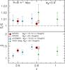 |
Fig. 16 Comparison among the values of |
Figure 17 is analogous to Fig. 16. It shows the values of and for galaxy subsamples extracted from VIPERS (red dots) and zCOSMOS (blue squares) using magnitude cuts brighter than before: MB = −19.7 − z − 5log (h) for VIPERS and MB = −19.72 − z − 5log (h) for zCOSMOS. Our results confirm those obtained with the fainter samples; the values of and for VIPERS galaxies agree with those of zCOSMOS galaxies in the redshift range in which the two analyses overlap. Non-linearity is detected at more than 1σ in the VIPERS sample alone. No comparison was made with the VVDS-Deep sample in this case since none of the subsamples analysed by M05 match these luminosity cuts.
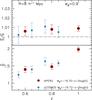 |
Fig. 17 Same as Fig. 16, but referring to brighter VIPERS (MB< −19.7 − z − 5log (h), red dots) and zCOSMOS galaxies (MB< −19.72 − z − 5log (h), blue squares). |
6.2. Linear bias from galaxy clustering
In Sect. 5 we saw that the bias of VIPERS galaxies deviates from linearity at all redshifts and on all scales explored. The amount of non-linearity, quantified by the parameter , is rather small, of the order of a few per cent. This means that is reasonably similar to bLIN and, therefore, can be compared with the linear bias parameter computed in other analyses.
In the following, we therefore compare the values of computed in this work with the values of bLIN obtained from different datasets in the same redshift range but using a variety of bias estimators. Galaxy bias at these redshifts has been estimated from both galaxy clustering and weak lensing. The latter probe, however, has either focused on bright objects used to trace baryonic acoustic oscillations (Comparat et al. 2013) or to explore bias dependence on the stellar mass (Jullo et al. 2012). Therefore, we focus on the values of bLIN obtained from galaxy clustering in other datasets available in the literature.
The results of these comparisons are shown in Fig. 18 in which we plot the most recent estimates of both and bLIN in the three redshift bins as a function of the magnitude cut. We consider the reference scale of R = 8h-1 Mpc since this is the size of the cells used to measure in VIPERS (large red circles), VVDS-Deep (small orange pentagons), and zCOSMOS (small, light green circles), as shown in the previous section. Magnitudes on the X-axis are specified in the B-band since this band is used in most of the considered samples with the exception of the PRIMUS and CHFTLS-wide. For these two latter cases, we consider the g-band magnitude and transform it into B-band according to the g − B versus z relation measured from the VIPERS catalogue. Finally, all results were normalised to σ8 = 0.9.
The large red circles represent the values obtained from VIPERS, for the systematic errors listed in Table 2. Therefore these values are slightly different from those shown in Figs. 16 and 17.
The light blue asterisks represent the bLIN values obtained from the Wide part of the Canada-France-Hawaii Legacy Survey (CFHTLS; Coupon et al. 2012). In this case, the bias values were computed from ~3 × 10⁶ galaxies in the redshift interval z = [0.2,1.2] by fitting a Halo Occupation Distribution model to the measured angular correlation function. These bLIN values were obtained by integrating the halo bias over the halo mass function. Therefore they are integral quantities much like , which is computed by integrating over the mass PDF (Eq. (2)). The bLIN values of CFHTLS galaxies agree well with our results in all redshift bins, including z = [0.9,1.1].
The brown crosses in the middle panel of Fig. 18 are from Skibba et al. (2014) and show the bias of galaxies in the PRIMUS catalogue. The PRIMUS (Coil et al. 2011) galaxy survey is carried out using a low-resolution spectrograph and complete down to i< 23. This dataset, which covers five independent fields (including the COSMOS field), spans the redshift range z = [0.2,1.0]. Here we focus on the interval z = [0.5,1.0] and plot the corresponding bias values in the middle panel. The bias was estimated from the projected galaxy 2-point correlation function, wp,g(r), as 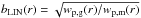 , where the projected 2-point correlation function of the matter, wp,m(r), was modelled assuming a flat ΛCDM model with σ8 = 0.8. The bias of PRIMUS galaxies is systematically larger than that of VIPERS. However, the significance of the mismatch is below 1σ.
The purple hexagons in the plot show bLIN of ALHAMBRA galaxies (Arnalte-Mur et al. 2014). The photometric redshift survey ALHAMBRA covers seven independent fields, including DEEP2 and COSMOS. Photometric redshifts are accurate enough to measure the projected galaxy correlation function at different redshifts and, from this, to estimate the bias. In Fig. 18 we show the bLIN values estimated in three redshift bins: [0.35,0.65] (top panel), [0.55,0.85] (middle panel), and [0.75,1.05] (bottom panel). We did not consider the interval z = [0.95,1.25] since it is largely beyond the VIPERS range. We show two sets of points. Small open hexagons represent the values of bLIN obtained from the clustering of galaxies in all seven fields (labelled ALHAMBRA+ in the plot). Filled hexagons (labelled ALHAMBRA-) illustrate the effect of removing two “outlier” fields, COSMOS and ELAIS-N1, which are characterised by a high degree of clustering. The bias of galaxies in ALHAMBRA- agrees with that of VIPERS for z< 0.9. In the last redshift bin, for MB(z = 1) < −20.56 − 5log (h) the bias of ALHAMBRA- is ~1.5σ below that of VIPERS. However, the discrepancy disappears when one considers ALHAMBRA+ and seems to reappear, with a reverse sign, at higher luminosities.
The green triangles show the bLIN values obtained from the projected galaxy 2-point correlation function of galaxies brighter than MB − 5log (h) = −20.5 − 5log (h) at z = [0.9,1.1] in the DEEP2 survey (Coil et al. 2006). In the brightest magnitude bin, where the three samples overlap, we find that the bias of DEEP2 galaxies is significantly smaller than that of VIPERS and ALHAMBRA objects.
To summarise, we find a good agreement between the value of measured in our work and those of bLIN estimated in a number of surveys in the range z = [0.5,0.9]. In particular, our measurements agree with those of K11 (small, light green circles) who used the same technique to estimate .
In the outermost redshift shell not all the bias values measured in different surveys agree with each other. The value of bLIN for DEEP2 and, to a lesser extent, for ALHAMBRA-galaxies, are smaller than from VIPERS. This mismatch may indicate either a genuine difference in the clustering properties of the different samples or deviations from linear bias highlighted by the different bias estimators.
To quantify the impact of non-linear bias, we compare our values with the corresponding bLIN estimated from the very same VIPERS subsamples considered here. Figure 19 compares from VIPERS (red filled symbols) with bLIN from Marulli et al. (2013; blue filled squares, also shown, for reference in Fig. 18). The two estimates agree at all redshifts but the last redshift bin where the bias of Marulli et al. (2013) matches that of DEEP2 galaxies and, consequently, is significantly below our value.
Like most of the other measurements, Marulli et al. (2013) estimated bLIN from the projected 2-point correlation function. More precisely, they averaged the correlation signal over the interval r = [1,10]h-1 Mpc . In the presence of a scaled dependent bias, a manifestation of which is a ratio different from unity, it is not obvious which effective scale of the bias is estimated by Marulli et al. (2013). In our comparison we implicitly assumed that this scale is the same as the cell size, i.e. 8 h-1 Mpc . In fact, a small scale seems more appropriate, especially if one accounts for the fact that errors in the projected correlation function increases with the pair separation. For this reason, we also show measured in cells of R = 6h-1 Mpc (orange hexagons). In this case, the significance of the mismatch is significantly reduced. Decreasing the scale to R = 4h-1 Mpc (not shown) would bring the two values into agreement at the price, however, of creating a mismatch at lower redshifts.
Focusing on the VIPERS sample, a more homogeneous comparison can be performed considering the bLIN value obtained by Cappi et al. (2015) from counts in cells of R = 8h-1 Mpc (brown asterisks, in the plots). In this case the results agree with ours within the (rather large) error bars.
In the figure we also show the VIPERS linear bias estimated by Granett et al. (2015; green triangles) from a Bayesian reconstruction of a Wiener filtered, adaptively smoothed galaxy density field. The result agrees with that of Marulli et al. (2013). However, as in that case, it is difficult to associate an effective scale to the filtering procedure and perform a homogeneous comparison with our estimate.
Therefore, all the bias estimates of the VIPERS galaxies agree with each other at z< 0.9, a sign that galaxy bias is largely independent of scales. At higher redshifts we observe some discrepancies among the various estimates whose significance, however, is difficult to assess since the different estimates are sensitive to different scales. It is safe to conclude that the scale-dependence bias of VIPERS galaxies is more pronounced at high redshifts, as confirmed by the results presented in Sect. 5.3, and that this can account for most of the discrepancies seen in Fig. 19.
An additional, though minor, source of discrepancy is incompleteness. At z ~ 1 the 90% completeness limit in VIPERS is MB − 5log (h) ~ −21.0 for red galaxies and about half a magnitude fainter for the blue galaxies. Since red galaxies are more biased than the blue galaxies, selecting objects at this luminosity cut underestimates the bias of the composite VIPERS sample. The amplitude of the effect depends on the luminosity cut. We conclude that deviations from linear bias cannot be ignored at high redshifts and that using bLIN as a proxy for galaxy bias leads to significant systematic errors.
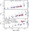 |
Fig. 18 Comparison between the bias parameters |
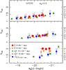 |
Fig. 19 Comparison between the bias parameter |
7. Discussion and conclusions
The importance of characterising galaxy bias at intermediate redshifts stems from the need to infer the properties of the distribution of the mass from that of the galaxies. This will be especially important in future redshift surveys aimed at an accurate estimate of the cosmological parameters. This has prompted several efforts to estimate galaxy bias at z> 0.5 exploiting weak lensing, galaxy clustering, and galaxy counts. Most of these works assume that galaxy bias is linear and deterministic and provide an estimate for the linear bias parameter. In this work we questioned this assumption and searched for possible deviations from linear bias. This issue has already been investigated by M05 and K11 (using counts in cells and significantly smaller samples) and by Simon et al. (2007) and Jullo et al. (2012) with conflicting evidence, as discussed in the introduction.
Our work builds upon these results improving the original strategy of M05 and K11 in several aspects. First of all, it is based on a new dataset of ~50 000 galaxies distributed over a much larger volume than its predecessors. This significantly reduces the impact of cosmic variance that in previous studies dominated the error budget. Secondly, we use a new technique to infer the mean biasing function from counts in cells that, under the hypothesis of local Poisson sampling, accounts and automatically corrects for shot noise. This improvement greatly increases our ability to recover the biasing function since Poisson noise is the main source of stochasticity in the bias relation. Thirdly, owing to the size of the sample, we are able to explore the bias dependence on magnitude, redshift, and scale with unprecedented accuracy. We postpone the investigation of additional dependences on galaxy colour and stellar mass to a future analysis to be performed with the final VIPERS sample and new mock galaxy catalogues designed to mimic these galaxy properties.
The main results of our study are:
The overall qualitative behaviour of the mean biasing function of VIPERS galaxies is similar to that of zCOSMOS and VVDS-Deep galaxies as well as to that of the synthetic VIPERS galaxies in the mock catalogues that we used to estimate errors. The shape of the mean biasing function is close to linear in regions above the mean density. It deviates from linear bias at δ< 0. More specifically, above the threshold δTH at which δg = −0.9, the bias function is significantly steeper than its mean slope on scales smaller than 8 h-1 Mpc . For over-densities below δTH the mean biasing function features a tail that cannot be accounted for by linear biasing. The over-density threshold δTH has been interpreted as a typical density scale below which very few galaxies form. In our analysis, we find that this threshold increases with the redshift and with the luminosity cut-of,f so that at moderate redshifts low-density regions are typically populated by faint galaxies.
The biasing function shows small but significant deviations from linearity at all redshifts, scales, and magnitude intervals that we explored. The parameter that we use to quantify non-linearity neither seems to evolve with the redshift nor to depend on the luminosity. A scale dependence is observed at low redshifts below 6 h-1 Mpc with only ~1σ significance.
We confirm that galaxy bias depends on luminosity. The mean slope of the biasing function, a good proxy to linear bias given the small degree of non-linearity, increases with the luminosity threshold used to select the galaxy sample. The effect is significant for z = [0.5,0.7], probably thanks to the large magnitude leverage here compared to the bin z = [0.9,1.1], in which we can probe a much smaller magnitude range ΔMB = 0.4. The value of δTH also increases with the magnitude, suggesting that the efficiency of galaxy formation decreases with the luminosity of the object.
We confirm that galaxy bias increases with redshifts as predicted by most bias models and verified in other datasets. In our case we find evidence for a rapid evolution beyond z = 0.9. This result is highly significant and robust since it depends neither on the scale nor on the luminosity of the objects. The statistical significance of this result depends on the reliability of our error analysis, which is based on a mock galaxy catalogue designed to match the correlation properties of VIPERS galaxies. We verified that mock catalogues are very realistic in the sense that their biasing function matches that of real objects remarkably well. In this analysis, we modelled all known sources of systematic errors, including the magnitude dependence of the spectroscopic sampling rate that was not originally included in the mock catalogues. We find no evidence for systematic errors that might mimic a spurious evolution in the bias moments and .
The value of increases with the scale from 4 to 8 h-1 Mpc . We interpret this in the framework of the halo model as the transition between the one-halo and two-halo contribution to galaxy bias. The same trend is seen in our mock catalogues, in which objects were extracted assuming the HOD model and in previous analyses performed at lower redshifts using both galaxy clustering (e.g. Zehavi et al. 2005) and weak lensing (e.g. Hoekstra et al. 2002; Simon et al. 2007). This is the first time that this effect is detected at high redshifts with counts in cells statistics.
We compared our results with those of M05 and K11. These authors performed an analysis similar to that presented here in a similar range of redshifts. We limited the comparison on a scale of 8 h-1 Mpc , which is common to the three analyses. We find that the values of of VIPERS and zCOSMOS galaxies agree within the errors. M05 find a smaller degree of biasing but the difference is of the order of 1 − σ. We conclude that the claimed discrepancy between K11 and M05 results is a manifestation of cosmic variance.
Deviations from linear biasing were also detected by M05 and K11, although with a lower significance than in our case. Our results agree with those of K11. In M05 the degree of non-linearity is slightly larger than in our case but the discrepancy is barely larger than 1σ. The bias non-linearity is sometimes expressed in terms of the parameter b2 of the second-order Tailor expansion of δ (Fry & Gaztanaga 1993). Cappi et al. (2015) analysed the same VIPERS dataset using higher order statistics, which is a procedure that is less sensitive to non-linear bias than ours. They detected a deviation from linear bias at z ≤ 0.9 with a significance of ~1σ. Their b2 value turned out to be negative, in agreement with M05 and Marinoni et al. (2008) and, qualitatively, with our results too. measured from the clustering of galaxies in recent galaxy redshift surveys (DEEP2, PRIMUS, CHFTLS-wide, and ALHAMBRA). This comparison is qualitative since it assumes that bias is linear, while our analysis has detected a small, but significant, degree of non-linearity in the bias of VIPERS galaxies. The comparison is generally successful at z< 0.9, where we find a very good agreement with all existing results. In this redshift range our results provide additional evidence in favour of a luminosity-dependent bias and of a weak evolution. At z> 0.9, where the spread among current results is large, our results favour the case of a significant bias evolution, in agreement with the CHFTLS-wide and ALHAMBRA analyses.
Our results confirm the importance of going beyond the simplistic linear biasing hypothesis. Galaxy bias is a complicated phenomenon. It can be non-deterministic, non-local, and non-linear. In this work we focused on deviations from linearity under the assumption that stochasticity is dominated by (and, consequently, accounted for) Poisson noise and that non-local effects are smoothed out within the volume of our cells. While the validity and the impact of these assumptions can (and will) need to be tested, our results show that the application of an improved statistical tool to the new VIPERS dataset is already able to detect deviations from linear bias with 5−10% accuracy.
Acknowledgments
We acknowledge the crucial contribution of the ESO staff for the management of service observations. In particular, we are deeply grateful to M. Hilker for his constant help and support of this programme. Italian participation in VIPERS is funded by INAF through PRIN 2008 and 2010 programmes. L.G. and B.R.G. acknowledge support of the European Research Council through the Darklight ERC Advanced Research Grant (# 291521). O.L.F. acknowledges support of the European Research Council through the EARLY ERC Advanced Research Grant (# 268107). Polish participants are supported by the Polish Ministry of Science (grant N N203 51 29 38), the Polish-Swiss Astro Project (co-financed by a grant from Switzerland, through the Swiss Contribution to the enlarged European Union), the European Associated Laboratory Astrophysics Poland-France HECOLS, and a Japan Society for the Promotion of Science (JSPS) Postdoctoral Fellowship for Foreign Researchers (P11802). G.D.L. acknowledges financial support from the European Research Council under the European Community’s Seventh Framework Programme (FP7/2007−2013)/ERC grant agreement No. 202781. W.J.P. and R.T. acknowledge financial support from the European Research Council under the European Community’s Seventh Framework Programme (FP7/2007−2013)/ERC grant agreement No. 202686. W.J.P. is also grateful for support from the UK Science and Technology Facilities Council through the grant ST/I001204/1. E.B., F.M., and L.M. acknowledge the support from grants ASI-INAF I/023/12/0 and PRIN MIUR 2010−2011. L.M. also acknowledges financial support from PRIN INAF 2012. Y.M. acknowledges support from CNRS/INSU (Institut National des Sciences de l’Univers) and the Programme National Galaxies et Cosmologie (PNCG). C.M. is grateful for support from specific project funding of the Institut Universitaire de France and the LABEX OCEVU. M.V. is supported by FP7-ERC grant “cosmoIGM” and by PD-INFN INDARK. C.D.P. wishes to thank Pangea Formazione S.r.l. for supporting her in the final stages of this work.
References
- Amara, A., Lilly, S., Kovač, K., et al. 2012, MNRAS, 424, 553 [NASA ADS] [CrossRef] [Google Scholar]
- Anderson, L., Aubourg, E., Bailey, S., et al. 2012, MNRAS, 427, 3435 [Google Scholar]
- Arnalte-Mur, P., Martínez, V. J., Norberg, P., et al. 2014, MNRAS, 441, 1783 [NASA ADS] [CrossRef] [Google Scholar]
- Basilakos, S., Plionis, M., Kovač, K., & Voglis, N. 2007, MNRAS, 378, 301 [NASA ADS] [CrossRef] [Google Scholar]
- Baugh, C. M. 2013, PASA, 30, 30 [Google Scholar]
- Bel, J., & Marinoni, C. 2014, A&A, 563, A36 [NASA ADS] [CrossRef] [EDP Sciences] [Google Scholar]
- Bel, J., Marinoni, C., Granett, B. R., et al. 2014, A&A, 563, A37 [NASA ADS] [CrossRef] [EDP Sciences] [Google Scholar]
- Bel, J., Branchini, E., Di Porto, C., et al. 2016, A&A, 588, A51 [NASA ADS] [CrossRef] [EDP Sciences] [Google Scholar]
- Blanton, M., Cen, R., Ostriker, J. P., Strauss, M. A., & Tegmark, M. 2000, ApJ, 531, 1 [NASA ADS] [CrossRef] [Google Scholar]
- Bottini, D., Garilli, B., Maccagni, D., et al. 2005, PASP, 117, 996 [NASA ADS] [CrossRef] [Google Scholar]
- Bower, R. G., Benson, A. J., Malbon, R., et al. 2006, MNRAS, 370, 645 [NASA ADS] [CrossRef] [Google Scholar]
- Branchini, E. 2001, ArXiv Astrophysics e-prints [arXiv:astro-ph/0110611] [Google Scholar]
- Cacciato, M., Lahav, O., van den Bosch, F. C., Hoekstra, H., & Dekel, A. 2012, MNRAS, 426, 566 [NASA ADS] [CrossRef] [Google Scholar]
- Cappi, A., Marulli, F., Bel, J., et al. 2015, A&A, 579, A70 [NASA ADS] [CrossRef] [EDP Sciences] [Google Scholar]
- Casas-Miranda, R., Mo, H. J., Sheth, R. K., & Boerner, G. 2002, MNRAS, 333, 730 [NASA ADS] [CrossRef] [Google Scholar]
- Chang, C., Pujol, A., Gaztanaga, E., et al. 2016, MNRAS, 459, 3203 [NASA ADS] [CrossRef] [Google Scholar]
- Coil, A. L., Blanton, M. R., Burles, S. M., et al. 2011, ApJ, 741, 8 [NASA ADS] [CrossRef] [Google Scholar]
- Coil, A. L., Newman, J. A., Cooper, M. C., et al. 2006, ApJ, 644, 671 [NASA ADS] [CrossRef] [Google Scholar]
- Coil, A. L., Newman, J. A., Croton, D., et al. 2008, ApJ, 672, 153 [NASA ADS] [CrossRef] [Google Scholar]
- Coles, P., & Jones, B. 1991, MNRAS, 248, 1 [NASA ADS] [CrossRef] [Google Scholar]
- Colless, M., Dalton, G., Maddox, S., et al. 2001, MNRAS, 328, 1039 [NASA ADS] [CrossRef] [Google Scholar]
- Colombi, S. 1994, ApJ, 435, 536 [NASA ADS] [CrossRef] [Google Scholar]
- Comparat, J., Jullo, E., Kneib, J.-P., et al. 2013, MNRAS, 433, 1146 [NASA ADS] [CrossRef] [Google Scholar]
- Conroy, C., Wechsler, R. H., & Kravtsov, A. V. 2006, ApJ, 647, 201 [NASA ADS] [CrossRef] [Google Scholar]
- Contreras, S., Baugh, C. M., Norberg, P., & Padilla, N. 2013, MNRAS, 432, 2717 [NASA ADS] [CrossRef] [Google Scholar]
- Cooray, A., & Sheth, R. 2002, Phys. Rept., 372, 1 [Google Scholar]
- Coupon, J., Kilbinger, M., McCracken, H. J., et al. 2012, A&A, 542, A5 [NASA ADS] [CrossRef] [EDP Sciences] [Google Scholar]
- Cucciati, O., Zamorani, G., Lemaux, B. C., et al. 2014, A&A, 570, A16 [NASA ADS] [CrossRef] [EDP Sciences] [Google Scholar]
- de la Torre, S., & Peacock, J. A. 2013, MNRAS, 435, 743 [NASA ADS] [CrossRef] [Google Scholar]
- de la Torre, S., Guzzo, L., Peacock, J. A., et al. 2013, A&A, 557, A54 [NASA ADS] [CrossRef] [EDP Sciences] [Google Scholar]
- De Lucia, G., & Blaizot, J. 2007, MNRAS, 375, 2 [NASA ADS] [CrossRef] [Google Scholar]
- Dekel, A., & Lahav, O. 1999, ApJ, 520, 24 [NASA ADS] [CrossRef] [MathSciNet] [Google Scholar]
- Di Porto, C., Amendola, L., & Branchini, E. 2012a, MNRAS, 419, 985 [NASA ADS] [CrossRef] [Google Scholar]
- Di Porto, C., Amendola, L., & Branchini, E. 2012b, MNRAS, 423, L97 [NASA ADS] [CrossRef] [Google Scholar]
- Fritz, A., Scodeggio, M., Ilbert, O., et al. 2014, A&A, 563, A92 [NASA ADS] [CrossRef] [EDP Sciences] [Google Scholar]
- Fry, J. N., & Gaztanaga, E. 1993, ApJ, 413, 447 [NASA ADS] [CrossRef] [Google Scholar]
- Garilli, B., Guzzo, L., Scodeggio, M., et al. 2014, A&A, 562, A23 [NASA ADS] [CrossRef] [EDP Sciences] [Google Scholar]
- Gaztañaga, E., Norberg, P., Baugh, C. M., & Croton, D. J. 2005, MNRAS, 364, 620 [NASA ADS] [CrossRef] [Google Scholar]
- Gaztañaga, E., Cabré, A., & Hui, L. 2009, MNRAS, 399, 1663 [NASA ADS] [CrossRef] [Google Scholar]
- Granett, B. R., Branchini, E., Guzzo, L., et al. 2015, A&A, 583, A61 [NASA ADS] [CrossRef] [EDP Sciences] [Google Scholar]
- Guzzo, L., Pierleoni, M., Meneux, B., et al. 2008, Nature, 451, 541 [NASA ADS] [CrossRef] [PubMed] [Google Scholar]
- Guzzo, L., Scodeggio, M., Garilli, B., et al. 2014, A&A, 566, A108 [NASA ADS] [CrossRef] [EDP Sciences] [Google Scholar]
- Hawkins, E., Maddox, S., Branchini, E., & Saunders, W. 2001, MNRAS, 325, 589 [NASA ADS] [CrossRef] [Google Scholar]
- Hoekstra, H., van Waerbeke, L., Gladders, M. D., Mellier, Y., & Yee, H. K. C. 2002, ApJ, 577, 604 [NASA ADS] [CrossRef] [Google Scholar]
- Jullo, E., Rhodes, J., Kiessling, A., et al. 2012, ApJ, 750, 37 [NASA ADS] [CrossRef] [Google Scholar]
- Kaiser, N. 1987, MNRAS, 227, 1 [NASA ADS] [CrossRef] [Google Scholar]
- Kayo, I., Suto, Y., Nichol, R. C., et al. 2004, PASJ, 56, 415 [NASA ADS] [CrossRef] [Google Scholar]
- Kofman, L., Bertschinger, E., Gelb, J. M., Nusser, A., & Dekel, A. 1994, ApJ, 420, 44 [NASA ADS] [CrossRef] [Google Scholar]
- Kovač, K., Porciani, C., Lilly, S. J., et al. 2011, ApJ, 731, 102 [NASA ADS] [CrossRef] [Google Scholar]
- Laureijs, R., Amiaux, J., Arduini, S., et al. 2011, ArXiv e-prints [arXiv:1110.3193] [Google Scholar]
- Le Fèvre, O., Saisse, M., Mancini, D., et al. 2003, in SPIE Conf. Ser., 4841, eds. M. Iye, & A. F. M. Moorwood, 1670 [Google Scholar]
- Manera, M., & Gaztañaga, E. 2011, MNRAS, 415, 383 [NASA ADS] [CrossRef] [Google Scholar]
- Marinoni, C., Le Fèvre, O., Meneux, B., et al. 2005, A&A, 442, 801 [NASA ADS] [CrossRef] [EDP Sciences] [Google Scholar]
- Marinoni, C., Guzzo, L., Cappi, A., et al. 2008, A&A, 487, 7 [NASA ADS] [CrossRef] [EDP Sciences] [Google Scholar]
- Marulli, F., Bolzonella, M., Branchini, E., et al. 2013, A&A, 557, A17 [NASA ADS] [CrossRef] [EDP Sciences] [Google Scholar]
- McCracken, H. J., Peacock, J. A., Guzzo, L., et al. 2007, ApJS, 172, 314 [NASA ADS] [CrossRef] [Google Scholar]
- Meneux, B., Le Fèvre, O., Guzzo, L., et al. 2006, A&A, 452, 387 [NASA ADS] [CrossRef] [EDP Sciences] [Google Scholar]
- Meneux, B., Guzzo, L., Garilli, B., et al. 2008, A&A, 478, 299 [NASA ADS] [CrossRef] [EDP Sciences] [Google Scholar]
- Meneux, B., Guzzo, L., de la Torre, S., et al. 2009, A&A, 505, 463 [NASA ADS] [CrossRef] [EDP Sciences] [Google Scholar]
- Mustapha, H., & Dimitrakopoulos, R. 2010, Comput. Geosc., 36, 313 [CrossRef] [Google Scholar]
- Nishimichi, T., Kayo, I., Hikage, C., et al. 2007, PASJ, 59, 93 [NASA ADS] [CrossRef] [Google Scholar]
- Norberg, P., Baugh, C. M., Hawkins, E., et al. 2001, MNRAS, 328, 64 [NASA ADS] [CrossRef] [Google Scholar]
- Norberg, P., Baugh, C. M., Hawkins, E., et al. 2002, MNRAS, 332, 827 [NASA ADS] [CrossRef] [Google Scholar]
- Nusser, A., Davis, M., & Branchini, E. 2014, ApJ, 788, 157 [NASA ADS] [CrossRef] [Google Scholar]
- Nuza, S. E., Sánchez, A. G., Prada, F., et al. 2013, MNRAS, 432, 743 [NASA ADS] [CrossRef] [Google Scholar]
- Percival, W. J., Cole, S., Eisenstein, D. J., et al. 2007, MNRAS, 381, 1053 [NASA ADS] [CrossRef] [MathSciNet] [Google Scholar]
- Pollo, A., Guzzo, L., Le Fèvre, O., et al. 2006, A&A, 451, 409 [NASA ADS] [CrossRef] [EDP Sciences] [Google Scholar]
- Prada, F., Klypin, A. A., Cuesta, A. J., Betancort-Rijo, J. E., & Primack, J. 2012, MNRAS, 423, 3018 [NASA ADS] [CrossRef] [Google Scholar]
- Pujol, A., Chang, C., Gaztañaga, E., et al. 2016, MNRAS, 462, 35 [NASA ADS] [CrossRef] [Google Scholar]
- Reid, B. A., Samushia, L., White, M., et al. 2012, MNRAS, 426, 2719 [NASA ADS] [CrossRef] [Google Scholar]
- Schlegel, D., Abdalla, F., Abraham, T., et al. 2011, ArXiv e-prints [arXiv:1106.1706] [Google Scholar]
- Scodeggio, M., Franzetti, P., Garilli, B., Le Fèvre, O., & Guzzo, L. 2009, The Messenger, 135, 13 [NASA ADS] [Google Scholar]
- Seo, H.-J., & Eisenstein, D. J. 2003, ApJ, 598, 720 [NASA ADS] [CrossRef] [Google Scholar]
- Sheth, R. K. 1995, MNRAS, 274, 213 [NASA ADS] [CrossRef] [Google Scholar]
- Sigad, Y., Branchini, E., & Dekel, A. 2000, ApJ, 540, 62 [NASA ADS] [CrossRef] [Google Scholar]
- Sigad, Y., Eldar, A., Dekel, A., Strauss, M. A., & Yahil, A. 1998, ApJ, 495, 516 [NASA ADS] [CrossRef] [Google Scholar]
- Simon, P., Hetterscheidt, M., Schirmer, M., et al. 2007, A&A, 461, 861 [NASA ADS] [CrossRef] [EDP Sciences] [Google Scholar]
- Skibba, R. A., Smith, M. S. M., Coil, A. L., et al. 2014, ApJ, 784, 128 [NASA ADS] [CrossRef] [Google Scholar]
- Somerville, R. S., Lemson, G., Kolatt, T. S., & Dekel, A. 2000, MNRAS, 316, 479 [NASA ADS] [CrossRef] [Google Scholar]
- Somerville, R. S., Lemson, G., Sigad, Y., et al. 2001, MNRAS, 320, 289 [NASA ADS] [CrossRef] [Google Scholar]
- Springel, V., White, S. D. M., Jenkins, A., et al. 2005, Nature, 435, 629 [NASA ADS] [CrossRef] [PubMed] [Google Scholar]
- Swanson, M. E. C., Tegmark, M., Blanton, M., & Zehavi, I. 2008, MNRAS, 385, 1635 [NASA ADS] [CrossRef] [Google Scholar]
- Szapudi, I., & Pan, J. 2004, ApJ, 602, 26 [NASA ADS] [CrossRef] [Google Scholar]
- Szapudi, I., Branchini, E., Frenk, C. S., Maddox, S., & Saunders, W. 2000, MNRAS, 318, L45 [NASA ADS] [CrossRef] [Google Scholar]
- Tegmark, M., & Bromley, B. C. 1999, ApJ, 518, L69 [NASA ADS] [CrossRef] [Google Scholar]
- Ueda, H., & Yokoyama, J. 1996, MNRAS, 280, 754 [NASA ADS] [CrossRef] [Google Scholar]
- Vale, A., & Ostriker, J. P. 2004, MNRAS, 353, 189 [Google Scholar]
- Verde, L., Heavens, A. F., Percival, W. J., et al. 2002, MNRAS, 335, 432 [NASA ADS] [CrossRef] [EDP Sciences] [Google Scholar]
- Viel, M., Branchini, E., Cen, R., et al. 2005, MNRAS, 360, 1110 [NASA ADS] [CrossRef] [Google Scholar]
- Villaescusa-Navarro, F., Marulli, F., Viel, M., et al. 2014, J. Cosm. Astro-Part. Phys., 3, 011 [CrossRef] [Google Scholar]
- Wang, Y. 2008, JCAP, 0805, 021 [Google Scholar]
- White, S. D. M., & Frenk, C. S. 1991, ApJ, 379, 52 [NASA ADS] [CrossRef] [Google Scholar]
- Wild, V., Peacock, J. A., Lahav, O., et al. 2005, MNRAS, 356, 247 [NASA ADS] [CrossRef] [Google Scholar]
- Yoshikawa, K., Taruya, A., Jing, Y. P., & Suto, Y. 2001, ApJ, 558, 520 [NASA ADS] [CrossRef] [Google Scholar]
- Zehavi, I., Blanton, M. R., Frieman, J. A., et al. 2002, ApJ, 571, 172 [NASA ADS] [CrossRef] [Google Scholar]
- Zehavi, I., Weinberg, D. H., Zheng, Z., et al. 2004, ApJ, 608, 16 [NASA ADS] [CrossRef] [Google Scholar]
- Zehavi, I., Zheng, Z., Weinberg, D. H., et al. 2005, ApJ, 630, 1 [Google Scholar]
- Zehavi, I., Zheng, Z., Weinberg, D. H., et al. 2011, ApJ, 736, 59 [NASA ADS] [CrossRef] [Google Scholar]
- Zheng, Z., Berlind, A. A., Weinberg, D. H., et al. 2005, ApJ, 633, 791 [NASA ADS] [CrossRef] [Google Scholar]
- Zucca, E., Bardelli, S., Bolzonella, M., et al. 2009, A&A, 508, 1217 [NASA ADS] [CrossRef] [EDP Sciences] [Google Scholar]
All Tables
All Figures
|
Fig. 1 Luminosity selection as a function of redshift. The black dots show the W1 and W4 VIPERS galaxies (with spectroscopic redshift flag between 2 and 9.5). Yellow lines represent the principal magnitude cuts applied in every redshift bin. The green line represents the cut M0 = −19.7 − z made to compare our results to those of K11. |
| In the text | |
|
Fig. 2 Reconstructed PDF of the mock VIPERS galaxies measured in cells of R = 4h-1 Mpc (top) and R = 8h-1 Mpc (bottom). The blue solid curve represents the reference galaxy PDF obtained by averaging over the PDFs reconstructed from the Parent mocks using the ΓE method. The blue dashed curve shows the average PDF reconstructed from the Realistic mocks using the same method. The blue shaded region represents the 1σ scatter among the 26 Realistic mocks. We plot P(1 + δg)(1 + δg) to highlight the performance of the reconstruction at high and low over-densities. We note the different Y-ranges in the two panels. The bottom panels in each plot show the difference Δp between the reconstructed and reference PDFs in units of the random error σp. Horizontal, dashed lines indicate systematic errors equal to 1σp random uncertainties. |
| In the text | |
|
Fig. 3 Mean biasing function of mock VIPERS galaxies computed from counts in cells of R = 4h-1 Mpc (bottom panel) and R = 8h-1 Mpc (top panel). The magnitude cut and redshift range of the mock VIPERS subsample, indicated in the plot, are the same as Fig. 2. Solid red curve: reference biasing function obtained from the Parent mock catalogues. Blue dashed curve and blue-shaded region: average value and 2σ scatter of the biasing function reconstructed from the Realistic mocks using the ΓE method. Brown dot-dashed curve and orange-shaded band: average value and 2σ scatter of the biasing function reconstructed from the Realistic mocks using a “direct” estimate of the galaxy PDF. Bottom sub-panels: difference Δp between the reconstructed and reference PDFs in units of the random error σp. Dashed lines indicate systematic errors equal to 1σp random errors. |
| In the text | |
|
Fig. 4 Solid red curve: reference mean biasing function of Fig. 3 computed using the mass PDF from N-body simulations. Brown dot-dashed curve and orange band: biasing function obtained using a lognormal fit to the mass PDF and 2σ scatter from the mocks. Blue dashed curve and blue band: biasing function obtained using a skewed lognormal fit to the mass PDF and 2σ scatter from the mocks. Bottom panels: difference Δp between the reconstructed and reference PDFs in units of the random error σp. Dashed lines indicate systematic errors equals to 1σp random errors. |
| In the text | |
|
Fig. 5 Mean biasing function estimated in real space (solid, red curve) and redshift space (dashed blue curve and its 2σ uncertainty band). Counts are performed in spherical cells with a radius of 4 h-1 Mpc . The luminosity cut and the redshift range is indicated in each panel. The width of each band represents the scatter among mocks. In the bottom part of each plot we show the difference Δp between the reconstructed and reference PDFs in units of σTOT, where σTOT accounts for the rms scatter in both the real- and redshift-space mocks. Dashed lines indicate where systematic errors equal to 1σTOT random errors. |
| In the text | |
|
Fig. 6 Bottom panel: per cent difference between the |
| In the text | |
|
Fig. 7 Mean biasing function of VIPERS galaxies from counts in cells of radius 6 h-1 Mpc as a function of the B-band magnitude cut in three redshift ranges indicated in each panel. Curves with different colours and line styles correspond to the different magnitude cuts indicated in upper panel. Error bars with matching colours represent the associated 1σ uncertainty intervals estimated from the mocks. A horizontal offset δ = 0.015 was applied to avoid overlapping error bars. All biasing functions are plotted out to δMAX. |
| In the text | |
|
Fig. 8 Zoom into the under-density range of Fig. 7. The horizontal short-dashed line represents the over-density threshold δg = −0.9. The long dashed line shows the linear biasing function |
| In the text | |
|
Fig. 9 Second-order moments of the mean biasing functions shown in Fig. 7. Left panels: moment |
| In the text | |
|
Fig. 10 Left: second-order moment |
| In the text | |
|
Fig. 11 Mean biasing function of VIPERS galaxies with MB< −19.5−z − 5log (h) measured in different redshift bins, characterised by different colours and line-styles, as indicated in the plot. Error bars represents the 1σ scatter in the mocks. The three panels refer to different cell sizes with radii R = 4,6,8h-1 Mpc from top to bottom. A horizontal offset δ = 0.015 was applied to avoid overlapping error bars. All curves are plotted out to δMAX. |
| In the text | |
|
Fig. 12 Moments of the mean biasing functions shown in Fig. 11. Panels from top to bottom indicate cells of increasing size. Left panels: |
| In the text | |
|
Fig. 13 Mean biasing function of VIPERS galaxies with MB< −19.5−z − 5log (h) computed from counts in cells with radii of 4,6, and 8h-1 Mpc . Biasing functions at different scales are indicated with different colours and line styles, as indicated in the plots. Error bars represent the 2σ rms scatter in the mocks. Different panels refer to different redshift shells. An offset δ = 0.015 was applied to avoid overlapping error bars. Curves are plotted out to δMAX. |
| In the text | |
|
Fig. 14 Moments of the mean biasing functions vs. the size of the cell. Panels from top to bottom refer to different redshift ranges indicated in the plot. Left panels: |
| In the text | |
|
Fig. 15 Bottom panel: comparison between |
| In the text | |
|
Fig. 16 Comparison among the values of |
| In the text | |
|
Fig. 17 Same as Fig. 16, but referring to brighter VIPERS (MB< −19.7 − z − 5log (h), red dots) and zCOSMOS galaxies (MB< −19.72 − z − 5log (h), blue squares). |
| In the text | |
|
Fig. 18 Comparison between the bias parameters |
| In the text | |
|
Fig. 19 Comparison between the bias parameter |
| In the text | |
Current usage metrics show cumulative count of Article Views (full-text article views including HTML views, PDF and ePub downloads, according to the available data) and Abstracts Views on Vision4Press platform.
Data correspond to usage on the plateform after 2015. The current usage metrics is available 48-96 hours after online publication and is updated daily on week days.
Initial download of the metrics may take a while.