| Issue |
A&A
Volume 584, December 2015
|
|
|---|---|---|
| Article Number | A92 | |
| Number of page(s) | 83 | |
| Section | Catalogs and data | |
| DOI | https://doi.org/10.1051/0004-6361/201424063 | |
| Published online | 26 November 2015 | |
Galactic cold cores
IV. Cold submillimetre sources: catalogue and statistical analysis⋆,⋆⋆,⋆⋆⋆
1 Department of Physics, PO Box 64, 00014, University of
Helsinki, Finland
2
Institut Utinam, CNRS UMR 6213, OSU THETA, Université de
Franche-Comté, 41bis avenue de l’Observatoire, 25000
Besançon,
France
e-mail: julien@obs-besancon.fr
3
Université de Toulouse, UPS-OMP, IRAP, 31028
Toulouse,
France
4
CNRS, IRAP, 9
Av. colonel Roche, BP
44346, 31028
Toulouse Cedex 4,
France
5
Finnish Centre for Astronomy with ESO (FINCA), University of
Turku, Väisäläntie
20, 21500
Piikkiö,
Finland
6
Laboratoire AIM, IRFU/Service d’Astrophysique − CEA/DSM −
CNRS −
Université Paris Diderot, Bât. 709, CEA-Saclay, 91191
Gif-sur-Yvette Cedex,
France
7 Loránd Eötvös University, Department of Astronomy, Pàzmàny
P.s. 1/a, 1117 Budapest (OTKA K62304), Hungary
8
LERMA, Observatoire de Paris, PSL Research University, CNRS, UMR
8112, 75014
Paris,
France
9
Sorbonne Universités, UPMC Univ. Paris 6, UMR 8112,
LERMA,
75005
Paris,
France
10
European Southern Observatory, Karl-Schwarzschild-Str. 2, 85748
Garching bei München,
Germany
11
IAS, Université Paris-Sud, 91405
Orsay Cedex,
France
12
IPAC, Caltech, Pasadena
CA
91125,
USA
13
LERMA, CNRS UMR 8112, Observatoire de Paris and École Normale
Supérieure, PSL Research University, 24 rue Lhomond, 75005
Paris,
France
14
Laboratoire AIM Paris-Saclay, CEA/DSM −
INSU/CNRS −
Université Paris Diderot, IRFU/SAp CEA-Saclay, 91191
Gif-sur-Yvette,
France
15
Aix Marseille Université, CNRS, LAM (Laboratoire d’Astrophysique
de Marseille) UMR 7326, 13388
Marseille,
France
16
The University of Tokyo, Komaba 3-8-1, Meguro, 153-8902
Tokyo,
Japan
Received: 24 April 2014
Accepted: 23 August 2015
Context. For the project Galactic cold cores, Herschel photometric observations were carried out as a follow-up of cold regions of interstellar clouds previously identified with the Planck satellite. The aim of the project is to derive the physical properties of the population of cold sources and to study its connection to ongoing and future star formation.
Aims. We build a catalogue of cold sources within the clouds in 116 fields observed with the Herschel PACS and SPIRE instruments. We wish to determine the general physical characteristics of the cold sources and to examine the correlations with their host cloud properties.
Methods. From Herschel data, we computed colour temperature and column density maps of the fields. We estimated the distance to the target clouds and provide both uncertainties and reliability flags for the distances. The getsources multiwavelength source extraction algorithm was employed to build a catalogue of several thousand cold sources. Mid-infrared data were used, along with colour and position criteria, to separate starless and protostellar sources. We also propose another classification method based on submillimetre temperature profiles. We analysed the statistical distributions of the physical properties of the source samples.
Results. We provide a catalogue of ~4000 cold sources within or near star forming clouds, most of which are located either in nearby molecular complexes (≲1 kpc) or in star forming regions of the nearby galactic arms (~2 kpc). About 70% of the sources have a size compatible with an individual core, and 35% of those sources are likely to be gravitationally bound. Significant statistical differences in physical properties are found between starless and protostellar sources, in column density versus dust temperature, mass versus size, and mass versus dust temperature diagrams. The core mass functions are very similar to those previously reported for other regions. On statistical grounds we find that gravitationally bound sources have higher background column densities (median Nbg(H2) ~ 5 × 1021 cm-2) than unbound sources (median Nbg(H2) ~ 3 × 1021 cm-2). These values of Nbg(H2) are higher for higher dust temperatures of the external layers of the parent cloud. However, only in a few cases do we find clear Nbg(H2) thresholds for the presence of cores. The dust temperatures of cloud external layers show clear variations with galactic location, as may the source temperatures.
Conclusions. Our data support a more complex view of star formation than in the simple idea of a column density threshold. They show a clear influence of the surrounding UV-visible radiation on how cores distribute in their host clouds with possible variations on the Galactic scale.
Key words: catalogs / submillimeter: ISM / stars: formation / ISM: clouds
Planck (http://www.esa.int/Planck) is a project of the European Space Agency − ESA − with instruments provided by two scientific consortia funded by ESA member states (in particular the lead countries: France and Italy) with contributions from NASA (USA), and telescope reflectors provided in a collaboration between ESA and a scientific consortium led and funded by Denmark.
Herschel is an ESA space observatory with science instruments provided by European-led Principal Investigator consortia and with important participation from NASA.
Full Table B.1 is only available at the CDS via anonymous ftp to cdsarc.u-strasbg.fr (130.79.128.5) or via http://cdsarc.u-strasbg.fr/viz-bin/qcat?J/A+A/584/A92
© ESO, 2015
1. Introduction
How stars form is one of the most central questions in astrophysics. It is closely related to major astrophysical problems, from galaxy structure, formation, and evolution to the dynamics and chemical evolution of the interstellar medium. It is a complex process resulting from the interplay between many physical phenomena including turbulence, magnetic fields, kinematics, and gravity. Despite this complexity, the main phases of the star formation process are understood well, starting from molecular clouds and progressing via dense cores down to protostellar collapse (McKee & Ostriker 2007). This knowledge has emerged from the detailed observations of the nearest low-mass and intermediate-mass star formation regions and, in addition, from sophisticated numerical modelling (Hennebelle et al. 2011; Padoan & Nordlund 2011). The next step in improving the overall view of star formation consists in understanding the process on the individual scale, and so extensive surveys of stars at different stages of their formation process and in different environments are required.
The earliest steps of star formation are of particular interest. How are the properties of the parent molecular cloud related to the characteristics of the forming stars? Can the star formation efficiency or the initial stellar mass function (IMF) be predicted from the observation of the parent cloud? General trends have been derived for star formation timescales and for the role played by the different physical processes (Federrath & Klessen 2012, and references therein). The central role of filaments and the existence of a threshold column density for cloud collapse have been emphasised (André et al. 2014). At the same time, star formation laws have been developed which relate the star formation rate with the available amount of dense gas (Kennicutt 1998; Lada et al. 2010). There are ongoing discussions about the variations in star formation laws from galaxy to galaxy and within the Milky Way (Daddi et al. 2010; Shetty et al. 2013; Federrath 2013) which show the need to understand the finer details in the interplay between processes and in the influence of the environment on star formation.
A new approach to the study of the earliest stages of star formation has been enabled by the Planck satellite (Tauber et al. 2010). This space telescope has mapped the whole sky at several submillimetre wavelengths with high sensitivity and small beam size (below 5′ at the highest frequencies), providing data for an all-sky inventory of the coldest structures of the interstellar medium. The cold (Tdust < 14 K) and compact (close to beam size) objects were listed in a catalogue containing more than 10 000 objects. This Cold Clump Catalogue of Planck Object (C3PO, see Planck Collaboration XXIII 2011) contains clumps which possibly host pre-stellar cores and starless cores at subparsec scales. Because of the limited resolution, it is dominated by ~1 pc sized clumps and also contains larger cloud structures extending up to tens of pc in size. However, the low temperatures of the objects ensures that only the denser, less evolved regions which are significantly shielded from the interstellar radiation field are included. The objects detected by Planck are likely to contain one or several cores, many of which will be pre-stellar or in early stages of protostellar evolution. This Planck survey constitutes the first unbiased census (in terms of sky coverage) of possible future star forming sites and provides a good starting point for global studies addressing the pre-stellar phase of cloud evolution. It was then further developed and led to the Planck Catalogue of Galactic Cold Clumps (PGCC, Planck Collaboration XXVIII 2015), which contains 13188 Galactic sources.
Within the Herschel open time key programme Galactic cold cores (Juvela et al. 2010), we have mapped selected Planck C3PO objects with the Herschel PACS1 and SPIRE2 instruments (100−500 μm, Poglitsch et al. 2010; Griffin et al. 2010). Thanks to its higher spatial resolution, Herschel (Pilbratt et al. 2010) makes it possible to examine the structure of the sources which gave rise to the Planck detections, often resolving the individual cores. The inclusion of shorter wavelengths (down to 100 μm) helps to determine the physical characteristics of the sources and their environments, and to investigate the properties of the interstellar dust grains. Our Herschel survey covers 116 fields between 12 arcmin and one degree in size and altogether approximately covers 390 individual Planck detections of cold clumps. Preliminary results of this follow-up were presented in Juvela et al. (2010; 2011, Papers I and II, respectively) from the Herschel science demonstration phase observations (for the fields PCC288, PCC249, and PCC550) and in Planck Collaboration XXII (2011) for a sample of ten Planck sources. Results for a larger set of the first 71 fields observed with the SPIRE instrument (250, 350, and 500 μm) were presented by Juvela et al. (2012, Paper III). This previous paper concentrated on the large-scale structure of the clouds and the general characteristics of the main clumps. Cloud morphology was found to be dominated by one or several filaments in about half of the cases, most fields showing at least some filamentary structures. These results are in line with the conclusions of other Herschel programs dedicated to star formation like the Gould Belt (André et al. 2010), HOBYS (Motte et al. 2010), or Hi-GAL (Molinari et al. 2010) surveys. Further analysis of filaments in our Herschel observations is conducted in another paper (Rivera-Ingraham et al. 2015). In addition, several studies are dedicated to individual sources or peculiar groups of sources in the Galactic cold cores programme: L1642 (Malinen et al. 2014), Polaris Bear (Ristorcelli et al., in prep.), GAL110-13 (Montillaud et al., in prep.), or high-latitude clouds (Rivera-Ingraham et al., in prep.). Dust properties and their evolution are also an important point of this programme and are studied both from a statistical point of view (Juvela et al. 2012) and on the scale of individual clouds in a similar manner to Ysard et al. (2013) in the case of L1506 (from the Gould Belt survey).
In this paper we present results for all the 116 fields in the programme, observed with both the PACS (100, 160 μm) and SPIRE (250, 350, 500 μm) instruments. The general properties of the fields are determined as indicators of the environment in which star formation takes place. We build a catalogue of submillimetre cold sources. We make use of the multiwavelength and multiscale source extraction algorithm getsources (Men’shchikov et al. 2012) to generate the source catalogue as objectively and reproducibly as possible. The catalogue is compared with mid-infrared (mid-IR) data, using colour and spatial criteria to separate starless sources from sources containing protostellar objects. Particular attention is given to the statistical properties of the sources and to how they compare to the properties of their host cloud.
The paper is structured as follows. The observations are presented in Sect. 2. The properties of observed fields are presented in Sect. 3. This includes the estimates of target distances, and the calculation of colour temperature and column density maps. In Sect. 4, a catalogue of cold sources is built, and the reliability and completeness of the catalogue are assessed. The statistical properties of the cold sources are discussed in Sect. 5. Section 6 analyses the relationships between source properties and the characteristics of their host cloud. The conclusions are presented in Sect. 7. The brightness, colour temperature, and column density maps of 22 fields are shown in Appendix G, along with the positions and shapes of the cold sources of our catalogue. The data for all 116 fields are available online in the Muffins database3.
2. Observations and data reduction
2.1. Target selection
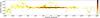 |
Fig. 1 Herschel fields of the Galactic Cold Cores programme shown in blue on the velocity-integrated CO map (Dame et al. 2001) of the Galaxy (colour scale, in K km s-1). Thirteen fields have absolute galactic latitude greater than 25 deg and do not appear on this map. |
For the Galactic Cold Cores programme, 116 fields were observed with the Herschel space observatory. Figure 1 shows their positions and extents plotted on the CO emission map of the Milky Way by Dame et al. (2001). The field selection was explained in detail in Paper III. In short, the Planck satellite (Tauber et al. 2010) all-sky submillimetre survey was analysed to build a catalogue of cold clumps, the C3PO, which contains more than 10 000 sources (Planck Collaboration XXIII 2011). A pre-selection of C3PO sources was performed on the basis of source binning upon galactic longitudes and latitudes, as well as dust colour temperature and mass estimates. This ensured a full coverage of the parameter ranges, putting special emphasis on rare source types (e.g. both ends of the clump mass spectrum) and the sky areas outside other planned surveys. The main objective was to build a coherent data set representing the entire cold core population of the Galaxy, complementing the other projects which target the most active star forming regions.
The final selection of 116 fields covers ~390 C3PO sources. A subset of 71 fields and their general properties was already presented in Paper III. In this paper we present for the first time the Herschel observations of an additional 45 fields; we use the whole set of 116 fields to study the properties of cold cores and, for the first time, present the PACS observations.
General properties of Herschel fields.
2.2. Herschel observations
The Photodetector Array Camera and Spectrometer (PACS) and Spectral and Photometric Imaging Receiver (SPIRE) instruments on board Herschel were used in photometric mode to acquire maps in the 100 and 160 μm PACS bands and in the 250, 350 and 500 μm SPIRE bands (with spatial resolutions of 7.7, 12, 18, 25, and 37′′, respectively) for the 116 fields listed in Table 1.
The SPIRE data were reduced with the Herschel interactive processing environment (HIPE) v.10.0, using the official pipeline4 with the iterative destriper and extended calibration options turned on. The zero-point correction was done outside HIPE as described in Paper III.
The PACS data were reduced both using HIPE v.10.0 and the version 18 of Scanamorphos (Roussel 2013). We found that Scanamorphos generally provides maps presenting fewer artefacts on large scales, and morphologies in closer agreement with SPIRE and WISE images than a HIPE-only map making (Madmap). In this paper, we use Scanamorphos maps for PACS and HIPE maps for SPIRE. The field G206.33-25.94-1 (IC 2118, the so-called Witch Head Nebula) was only observed with SPIRE.
Turn-around data were included both for SPIRE and PACS data in order to maximise the area of the maps. The surface brightness zero-points were derived using the method presented in Paper III.
2.3. Other data
We complemented our set of data with mid-IR and CO line emission data. The Wide-Field Infrared Survey Explorer (WISE) satellite (Wright et al. 2010) has four bands centred at 3.4, 4.6, 12.0, and 22.0 μm with spatial resolutions ranging from 6.1′′ at the shortest wavelength to 12′′ at 22 μm. WISE is an all-sky survey and therefore provides data for all 116 fields. We use these data to characterise the mid-infrared dust emission and to look for indications of ongoing star formation (see Sect. 4.4). The data were converted to surface brightness units with the conversion factors given in the explanatory supplement (Cutri et al. 2011). The calibration uncertainty is ~6% for the 22 μm band and less for the shorter wavelengths.
The AKARI mission (Murakami et al. 2007) also provides an all-sky survey in the mid- and far-IR domains. In Sect. 4.4 the AKARI point source catalogue (Yamamura et al. 2010) is used to classify sources in terms of evolutionary stage.
We use the CO J = 1−0 rotational line at 115 GHz from the survey by Dame et al. (2001). The relatively low spatial resolution of these data (8.5′) still enables various structures to be disentangled within our Herschel fields, while radial velocities (spectral resolution of 2 km s-1) are used to identify multiple components along the line of sight and to evaluate their kinematic distances (see Sect. 3.1). The survey covers about one-fifth of the sky, and part of the area is not fully sampled. Among our fields, 38 are covered by the fully sampled part of the survey, 57 by the partially sampled part, and 21 are not covered at all.
Wu et al. (2012) observed the J = 1−0 CO line towards 674 Planck clumps using the Purple Mountain Observatory 13.7 m telescope. Only 44 of our fields host sources observed by these authors. We use these radial velocity measurements to complement the data of Dame et al. (2001) to estimate source distances in Sect. 3.1. Finally, only 18 fields remain without known CO line measurements.
3. Field properties
3.1. Determination of distances
To derive the core properties, distance is one of the most crucial pieces of information. Many methods have been developed to estimate distances of molecular clouds. Parallax measurements of maser emission is the most reliable method as it minimises the number of astronomical assumptions (Foster et al. 2012). However, there are only a few maser parallax measurements, and current efforts to increase their number (e.g. BeSSeL project, Brunthaler et al. 2011) are naturally focused on high-mass star forming regions, more prone to maser emission. Therefore, very few of our fields have known maser emission, and none of them has a parallax measurement. Several other methods can be used to evaluate distances, like the extinction method, the kinematic method, and association with structures of known distance. These methods can also be combined to produce more reliable distance estimates (Ellsworth-Bowers et al. 2013, 2015). We present here the methods we used to produce distance estimates, as well as the general strategy to adopt a single distance estimate for each field. A field-by-field discussion is provided in Appendix D, and the distance estimates from all available methods are summarised in Fig. 2 and in Table D.1. The correlation between the various methods is summarised in Fig. D.1.
3.1.1. Extinction method
Stellar observations are subject to the extinction of interstellar dust which has the effect of making the observed colour indices redder than they would be in the absence of extinction. By comparing observed stellar colours to the predictions of the Besançon Galactic model (Robin et al. 2003, 2012), we attempt to infer the most probable 3D extinction distribution along the line of sight. Stars that lie within some area of the cloud are chosen from the Two Micron All Sky Survey (2MASS, Skrutskie et al. 2006) point source catalogue so that the location of the cloud along the line of sight should be detectable as a sharp rise in extinction. The principle of the method is the same as that described by Marshall et al. (2006, 2009), but with the modifications discussed below and presented more fully in Marshall et al. (in prep.).
The present version of the code explores the parameter space via a Markov chain Monte Carlo (MCMC) method and returns not only the most likely line-of-sight extinction, but also provides an estimate of the uncertainty. A further change is that the goodness of fit measurement has been updated from a χ2 test on the difference between the observed and modelled stellar colour histograms to a Kolmogorov-Smirnov test on the cumulative distribution function of the two colour-distributions. The Kolmogorov-Smirnov test is not sensitive to the histogram binning and performs better in the presence of fewer stars than the χ2 test.
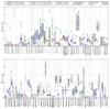 |
Fig. 2 Distance estimates for 108 of the 116 fields observed for the Galactic Cold Cores programme. The values and their associated uncertainties adopted in this paper are shown by the horizontal red lines and the grey areas, respectively. Fields with a reliable value-uncertainty pair (distance flag = 2) are in bold text. Grey text indicates fields with unreliable or no final estimates (distance flag = 0). No data could be found or produced for the five missing fields (G71.27-11.32, G128.78-69.46, G171.35-38.28, G218.06+2.12, and G299.57+5.61). For each field, all available estimates are shown. Stars with different colours indicate data found in the literature. The various methods are colour coded as presented in the upper panel and explained in Sect. 3.1. All numerical values are given in Table D.1, and individual sources are discussed in Appendix D. |
The resultant extinction versus distance profile is then analysed to detect the presence of any clouds. The dust density with respect to distance is calculated via the derivative of the extinction-distance relation and the diffuse extinction is estimated from the continuum. Any peaks in dust density 3σ over the diffuse extinction are flagged. If a line of sight contains more than one cloud, the one with the highest extinction is chosen. Only lines of sight with a single detected cloud have been included in the present sample.
In each field we applied this method to two circular areas with 5 and 10 arcmin in diameter, respectively, both centred on the brightest position. These positions were determined from the 250 μm brightness maps, after convolution with a Gaussian kernel with FWHM (full width at half maximum) of 5 arcmin, and excluding the positions closer than 10 arcmin from the edges of the maps. The distance estimates derived with this method are shown as blue filled circles in Fig. 2. In Table D.1 we give the distance estimates along with the number of 2MASS stars found in the two circular areas, the probability that the observed and modelled star populations come from the same parent distributions, and the significance of the cloud extinction detection. The main limitations of the extinction method come from the need to observe a large number of stars (≳100) in the direction of the cloud. Because our clouds have relatively high galactic latitudes (| b | ≳ 2 deg), this forces us to use large areas where the clouds may have uneven column density, leading to scatter in background star reddening.
3.1.2. Kinematic distances
Distances can be derived from spectroscopic observations, assuming galactic gas is in circular rotation (Reid et al. 2009; Dunham et al. 2011; Wienen et al. 2012, 2015). For this method to be reliable, the velocity of the cloud relative to the observer must be dominated by its rotation around the Galaxy. The peculiar velocity of nearby clouds is generally dominant and the kinematic method is considered reliable for distances greater than ~1 kpc. Kinematic distance estimates are unreliable for high galactic latitude clouds, because they are either nearby clouds, or lie far from the Galactic plane. In the latter case, they may have large peculiar velocities and are therefore unlikely to closely follow the galactic rotation curve. For clouds with galactic longitude close to 0 or 180 deg, the velocity component due to the rotation of the Galaxy is orthogonal to the line of sight and cannot be observed using spectroscopy. For these reasons, the kinematic distances of the 43 clouds with galactic latitude |b| > 10 deg or galactic longitude between 170 and 190 deg or between 350 and 10 deg were not considered.
Reid et al. (2009) report that massive star forming regions on average orbit the Galaxy ≈15 km s-1 slower than expected for circular orbits. It is unclear whether this result applies to some of our fields. To assess the impact of this uncertainty, the kinematic distances were computed both assuming zero peculiar velocity and a peculiar velocity of 15 km s-1 against the rotation of the Galaxy. The impact of the peculiar velocity varies greatly from field to field. It can be moderate as for G343.64-2.31 with a difference of 450 pc (~30%), but it is most often large and sometimes dramatic when the measured Vlsr is close to 15 km s-1. This is the case of G70.10-1.69 where a peculiar velocity v = 0 km s-1 leads to d = 80 pc, whereas v = 15 km s-1 leads to d = 2.81 kpc.
Most of our fields are covered by the CO survey of the Galaxy by Dame et al. (2001). In each field, we extracted the CO spectrum of the brightest submillimetre clump and determined the radial velocity of the cloud using Gaussian fitting of the CO lines. The kinematic distances were then derived using the rotation curve of Reid et al. (2009). More up to date parameters of the galactic rotation curve can be found in the recent work by Reid et al. (2014), but we do not use them because it would only change our distance estimates very marginally. The spectral resolution in the Dame et al. (2001) data goes from 0.26 km s-1 to 1.30 km s-1 with a value of 0.65 km s-1 for most lines of sight. For the sake of simplicity, we assumed an uncertainty of 1 km s-1 to estimate the uncertainties on kinematic distances with the rotation curve of Reid et al. (2009). The values of velocity, distance, and distance uncertainty are given in Table D.1. In a few cases, several components are seen, indicating that several clouds at different distances can be seen in the same field. In these cases, we report all the different distances in Table D.1 and in Fig. 2.
For some (43) fields, dedicated observations of 12CO were reported by Wu et al. (2012). The authors provide the values of velocity from Gaussian fitting of CO lines, as well as kinematic distance estimates. However, they used the older rotation curve of Clemens (1985) and for the sake of consistency, we recomputed the kinematic distance estimates based on the work of Reid et al. (2009).
These observations by Wu et al. (2012) are a good opportunity to check whether the data from the survey of Dame et al. (2001) can be associated with our higher resolution Herschel data, despite the low spatial resolution (~7 arcmin) and the poor spatial sampling of the survey. Figure 2 shows that the agreement between the two sets of observations is generally within the error bars. This gives us confidence in using the CO survey of Dame et al. (2001) when no dedicated molecular observations are available.
3.1.3. Other methods
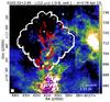 |
Fig. 3 Example of association between a Herschel target and an object with known distance in the case of the field G202.02+2.85 apparently connected with the stellar open cluster NGC 2264. The colour scale shows the relative intensity in the WISE 12 μm band. White and red contours are 0 and 100 MJy intensity levels from the Herschel 250 μm band and emphasise the map edges and the submillimetre mapped filament, respectively. The purple stars are those associated with NGC 2264 according to the SIMBAD database. |
In addition to these methods, we considered the distance estimates by associating the sources with structures for which distance estimates are already available in the literature. However, very different levels of accuracy were found in the literature. In addition, the association with our cloud is not always clear. When the associated object is a molecular cloud, we examined the IRAS 100 μm maps to evaluate the relevance of the association. For associations with stars, we checked DSS or WISE images for some indication of a connection, like the presence of a reflection nebula. For example, looking at either IRAS 100 μm or WISE 12 μm images (Fig. 3) strongly suggests that the filament mapped in the field G202.02+2.85 is connected with the open cluster NGC 2264 thanks to multiple reflection nebulae and a complex network of filaments which link the main filament observed with Herschel with the reflection nebulae. The values and their uncertainties are reported in Fig. 2 and in Table D.1 which also lists the relevant references.
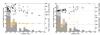 |
Fig. 4 Left: Galactic latitudes (orange points) and altitudes (black points) of our fields compared to the histogram of field distances. Open circles are for fields with unreliable distance estimates. Broken lines show the average values over distance bins. The contribution of fields with unreliable distance estimates to the distance histogram is shown in light grey. Right: same as left but for galactic longitude (orange) and galactic radius (black). |
3.1.4. Adopted distances
The adopted distances are given in Table 1. Figure 2 compares the available distance estimates for all methods, and gives the adopted values and their associated uncertainty. We did not try to classify the methods to identify the best one. Instead we examined each field individually to provide the best estimate considering the available data. A short discussion is provided for each field in Appendix D where we explain our choices of distance estimates. All the numbers are gathered in Table D.1. For a score of fields we propose estimates that differ from those proposed in Paper III, mostly because of more up-to-date references. For example, in Paper III the fields associated with the California nebula were attributed a distance of 350 pc, in reference to the work by Bohnenstengel & Wendker (1976). We now prefer the distance of 450 ± 23 pc, as derived by Lada et al. (2009).
We propose flags to indicate the level of confidence of the distance and uncertainty pairs, as given in Table 1. A flag equal to 2 was attributed to the 35 fields with a good level of confidence due to the agreement between different methods. A value of 1 indicates a reasonable estimate which needs to be confirmed by an independent method and was attributed to 44 fields. A value of 0 was attributed to the 29 fields with unreliable estimates which need to be excluded from any analysis sensitive to the value of distance. For three fields, the data did not enable a distance estimate to be derived, and no data could be found or produced for the remaining five fields.
3.2. Galactic distribution of Herschel fields
From the distances and coordinates, we computed the absolute galactic positions of our fields. The results are summarised in Fig. 4 and Table 1. Most fields have heliocentric distances less than 1.5 kpc. A wide range of galactic altitudes is covered by our sample, from 300 pc below to 200 pc above the Galactic plane; galactic latitudes only weakly correlate with galactic altitudes due to the effect of distance. It is more difficult to probe a wide range of galactic radii because, at large distances, observations are limited by instrumental resolution and sensitivity and by confusion. Nevertheless, our sample enables a 2 kpc range around the Sun to be covered with dozens of fields.
In Fig. 5 we show the estimated location of each target cloud in the Galactic plane viewed from the north Galactic pole. As discussed for each field individually in Appendix D, it appears that most observed clouds are either part of a nearby molecular complex (e.g. the California nebula for G157.08-8.68) or part of the Perseus Galactic arm (e.g. G139.60-3.06), and possibly the Carina-Sagittarius arm.
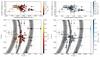 |
Fig. 5 90% percentile of dust temperature T90% (left) and median column density (right) of fields as functions of position in the Galaxy. In the lower panels, the X and Y coordinates define positions in the Galactic plane with the Galactic centre at (X,Y) = (0,0), the Sun at (X,Y) = (8400 pc,0), and 0 ≤ l ≤ 180 deg for Y ≤ 0. The shaded arcs are the Carina-Sagittarius arm (I), the local arm (II), and the Perseus arm (III), as parametrised by Hou & Han (2014, their Table 1, three-arm model with all spiral tracers). |
3.3. Temperature maps
We built the colour temperature maps of the large grain emission using the 250, 350, and 500 μm SPIRE maps, to visualise the location of the coldest clumps and reveal a possible external illumination of the cloud. Because we only use SPIRE data, the derived temperatures may not be very accurate in regions with temperatures close to 20 K or higher, for which dust emission peaks at wavelengths shorter than 250 μm. On the other hand, if PACS data were also included, temperature variations along the line of sight might bias the temperature estimates (Shetty et al. 2009a,b; Malinen et al. 2011). Another reason to exclude the 100 μm data is that it contains an unknown contribution from stochastically heated grains.
The colour temperature maps were computed using the following procedure. We convolved the maps to a resolution of 40′′ and, for each pixel, the SED was fitted with a modified black-body Bν(Tdust)νβ keeping the spectral index β at a fixed value of 2.0. The limitations of this procedure were already discussed by Juvela et al. (2012) who used Monte Carlo simulations and quantified the statistical error on temperature estimates. They found this error to be below 1 K in cold regions and ~3 K in warm regions (~20 K) when using only SPIRE data. Similarly, Juvela et al. (2012) used Monte Carlo simulations to evaluate how the uncertainty on the intensity zero points affects the temperature estimates. They found uncertainties of ~0.5 K in most fields, and up to ~1 K in a few fields.
We estimated the coldest dust temperatures in each map from the 0.1% percentile dust temperature5 T0.1%. The values are reported in Table 1. They range from T0.1% = 8.8 K to T0.1% = 16.6 K with a median value of 13.4 K. The use of the 0.1% percentiles instead of the minimum values prevents the possible outlier pixels from biasing the temperature values. We show these estimates because they are indicative of the coldest dust emission in a field and enable a quick comparison between fields. Nevertheless, they most likely overestimate the real minimum temperature because of the temperature variations along the line of sight. More accurate minimum dust temperatures are provided for individual sources using aperture photometry in Sects. 4.2 and 5.3.
Figure 5 summarises the variations in the 90% percentile dust temperature of fields T90% from field to field as a function of the position inside the galaxy. We expect this value to be an indication of the dust temperature in the outer layers of clouds and therefore of the intensity of the surrounding radiation field. We obtain values between T90% = 13.7 K and T90% = 24.5 K with a median value of 16.13 K. The value of T90% shows, on average, higher temperatures (~16−19K) for lower galactocentric distances (dgal ≲ 8 kpc), and lower temperatures (~14−17K) for dgal ≳ 9 kpc. We evaluated the temperature gradient in T90% with Galactic radius using a simple linear fit taking the distance uncertainties into account. Only clouds with distance quality flags of 1 and 2 were included. We also excluded fields with distances below a limit dmin because nearby fields tend to introduce noise in the fit whereas they do not provide much information on temperature gradient on the Galactic scale. The obtained gradient values depend somewhat on the value of dmin with values of ~−2.5 K kpc-1 for dmin < 1 kpc and ~−1.5 K kpc-1 for dmin > 1 kpc. Averaging over the values obtained for dmin between 300 pc and 2.0 kpc, we estimate the gradient in T90% with Galactic radius to be −1.9 ± 0.6 K kpc-1. This trend is consistent with the interstellar radiation field being more intense in the inner parts of the Galaxy, and therefore tends to confirm that T90% is a good proxy of the intensity of the surrounding visible-UV radiation field.
Interestingly, fields without a distance estimate tend to have significantly warmer outer temperature (T90% ~ 20−25 K) and lower median column densities (N(H2) ~ 1019−20 cm-2) than other fields. This is consistent with these fields having less clear extinction and CO signatures, and therefore being more challenging for distance estimation.
3.4. Column density maps and masses
We calculated the column density maps averaged over a 40′′ beam using the following formula for each pixel independently, 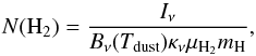 (1)where the intensity Iν and dust temperature Tdust are taken from the SED fitting described in Sect. 3.3, and μH2 = 2.8 is the mean particle mass per hydrogen molecule. For the dust opacity κν, we used the formula 0.1 cm2/ g (ν/ 1000 GHz)β which is suited to high density environments (Beckwith et al. 1990). The exact value of dust opacity is uncertain and varies with the environment according to grain evolution. Variations of the order of a factor of two are reported in κν from region to region (Boulanger et al. 1996) and within regions (Martin et al. 2012). Still, we follow Juvela et al. (2012) for choosing the value of the opacity, since it is consistent with predictions and observations of dense clouds (e.g. Ossenkopf & Henning 1994; Nutter et al. 2006, 2008) and is also the value used in Planck Collaboration XXIII (2011) and Planck Collaboration XXII (2011). The median values of column density N(H2)50% in all fields are given in Table 1. They range from N(H2)50% ~ 6 × 1019 cm-2 to N(H2)50% ~ 6 × 1021 cm-2 with a median value of N(H2)50% of 1.1 × 1021 cm-2.
The column density maps were derived using only SPIRE data and are shown in frame h of Fig. 6 for the field G176.27-2.09, and for 22 fields in Appendix G, and for all fields in the Muffins database. Figure 5 shows the variations in the median column density of the fields as a function of their galactic position. Contrary to dust temperature, no obvious trend is revealed against galactic radius or galactic altitude.
From the column density maps we derived the total masses in each field, defined as the sum of the masses in all the pixels of the field. For each pixel the mass was obtained from 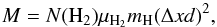 (2)where Δx is the pixel angular size and d is the cloud estimated distance. They are given in Table 1, and scatter between ~4 M⊙ (G141.25+34.37) and ~105M⊙ (G111.41-2.95). This shows that our sample of clouds contains objects very different in nature, from nearby small and tenuous clouds to large and distant molecular complexes. Some values differ from those given in Paper III because of new distance estimates (e.g. G21.16+12.11). Our fields are outside the Galactic plane, so the foreground and background contaminations are expected to be low. Nevertheless, in regions where some contamination exist, these estimates provide reasonable upper limits to the mass of the clouds of interest. On the other hand, in regions free of contamination, these masses may underestimate the real mass of clouds because part of the coldest dust grains can be missed by far-IR observations with 500 μm as the longest wavelength (Pagani et al. 2004).
4. Building a catalogue of cold sources
In this section, we aim to provide a list of the Herschel sources that are relevant for star formation studies, along with their main physical properties. We give details on the method used to extract the sources, to derive their physical properties, to identify the potential extragalactic sources, and to disentangle between starless and protostellar sources. We also assess the completeness of our catalogue. However, we do not make assumptions about the actual prestellar6 nature of our sources. We provide a dust-emission-based analysis of the physical nature and potential prestellar character of our sources in Sect. 5. Nevertheless, for the sake of completeness, we prefer to include in our source catalogue all the reliable submillimetre detections. Thus, in this section, we employ the general term of “source” rather than “core” or “clump”.
4.1. Extraction of sources
 |
Fig. 6 Data on the field G176.27-2.09. Shown are the surface brightness maps for WISE 22 μm (frame a), 12′′ resolution), PACS 100 μm (frame b), 7.7′′ resolution), PACS 160 μm (frame c), 12′′ resolution), SPIRE 250 μm (frame d), 18.1′′ resolution), SPIRE 350 μm (frame e), 25.2′′ resolution), and SPIRE 500 μm (frame f), 38.5′′ resolution). The dust colour temperature map (frame g), 40′′ resolution) and H2 column density map (frame h), 40′′ resolution) are derived from SPIRE data. The beam sizes are indicated in the lower left corner of each frame. The FWHM ellipses of sources are shown in frame i) plotted on the SPIRE 250 μm map. Candidate galaxies, protostellar, and starless sources are indicated with white triangles, red stars, and blue filled circles, respectively. Ellipses without additional symbols are galactic sources at an undetermined stage of evolution. The red ellipses in frame e) show the positions of Planck sources from the PGCC catalogue (Planck Collaboration XXVIII 2015). In frames c)−f), and h), the white solid line shows the boundary of the mask employed for the source extraction. |
We extracted the compact sources from Herschel data using the multiscale, multiwavelength algorithm getsources (version v1.130401, Men’shchikov et al. 2012), a source extraction method developed for Herschel Gould Belt survey (André et al. 2010) and Herschel HOBYS survey (Motte et al. 2010). This algorithm was designed to automatically locate compact sources (not necessarily point sources) in several maps simultaneously, to distinguish between background and source emission, and to characterise the sources quantitatively in a reproducible manner. Among other data, 2D Gaussian fits of source emission in each map are produced. Before performing the extractions, the brightness maps were colour corrected using the dust temperature maps derived from SPIRE maps, as explained in Sect. 3.3. All maps were then convolved with a Gaussian kernel to get an identical resolution of 38.5′′ in all bands. Spatial information on small scales is lost in the convolution process, but the extractions proved to be much more reliable on convolved maps than with the original resolutions. More importantly, having the same resolution for each band ensures that fluxes are measured in similar apertures and therefore helps to ensure that the emission comes from the same layers of the observed cloud. Finally, in each map the median value of the map was removed from pixel values. In principle, this change in offset value does not affect the results of aperture photometry, but in practice it ensures a better accuracy during the source extraction process (Men’shchikov, priv. comm.). The removed values were stored to enable the analysis of background column density from the background maps produced by getsources (Sect. 5.5).
The set of maps used to perform the extractions contains the PACS 160 μm, the SPIRE 250, 350 and 500 μm, and the column density maps presented in Sect. 3.4. Using this additional data opens the possibility of directly using getsources to evaluate whether the sources correspond to an increase in the column density on the plane of the sky and to measure their column density properties. Apart from a few fields, the PACS 100 μm maps proved to have low signal-to-noise ratios and were excluded. The other maps were used both as detection and measurement maps.
The getsources algorithm requires the user to provide masks to select the area of interest in each band. The number, positions, and characteristics of the extracted sources substantially depend on the shape and extent of these masks. The procedure to build the masks was automatised in an attempt to obtain a homogeneous set of extractions. However, for a few fields, the extractions were not satisfying, and some masks were modified manually to adapt to specific features. The masks used are shown in Fig. 6 for G176.27-2.09, for 22 fields in Appendix G, and for all fields in the Muffins database.
Relative alignment is critical for the accuracy of the measurements of source properties. We controlled the accuracy of the alignment by comparing the positions of point sources in monochromatic catalogues produced by getsources. The relative alignment is better than 5′′, which is small compared to the 38.5′′ resolution of our maps.
We used the default values for all parameters. From the wealth of sources extracted by getsources, we selected the most reliable using the flags generated by the algorithm. We required the following criteria to be fulfilled:
-
global goodness > 1,
-
high monochromatic significance (SIG_MONO>3.5) for SPIRE bands or column density maps,
-
measurable peak intensity (FXP_BEST/FXP_ERRO>1.0) for all SPIRE bands and column density maps,
-
measurable total flux (FXT_BEST/FXT_ERRO>1.0) for all SPIRE bands and column density maps.
We did not exclude sources with problematic detection (i.e. non-detection or low significance detection) at 160 μm, because the area of PACS maps is smaller than the area of SPIRE maps and many genuine sources are problematic at 160 μm. Also, for very cold sources (Tdust< 10 K) the flux is not expected to be measurable at PACS wavelengths. Still, requesting good detections simultaneously in all SPIRE bands and in the column density maps is a conservative approach and ensures a better reliability of the detections.
With this method, we obtain a catalogue of 4466 submillimetre sources, combining the detections in all the targeted fields. This catalogue contains different types of objects, from actual prestellar cold cores to extragalactic objects, and local column density maxima with lower density than actual cores. Further filtering is therefore needed.
4.2. Physical properties of the sources
A wealth of information on sources is provided by getsources. In the following we make use of the position, position angle, and size (major and minor axis) of the source elliptical full width half maximum (FWHM), the total flux attributed to the source in each photometric band and the uncertainties of these fluxes.
Using getsources total fluxes, we constructed the spectral energy distribution (SED) of each source. Assuming a single temperature for dust emission, we fitted the SED of each source with a modified black-body Bν(Tdust)νβ with the spectral index β fixed at a value of 2, as in Sect. 3.3. We thereby derived for each source the dust colour temperature Tdust. The mean column density was then computed from 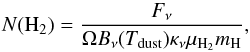 (3)where we used the flux Fν (total flux of the source in Jy, computed from the fitted function) and the temperature Tdust obtained from the SED fitting, the solid angle Ω corresponds to the source FWHM in the SPIRE 250 μm band, and κν is the same as in Sect. 3.4. Similarly the source mass was obtained from
  (4)where d is the distance of the source. The bolometric luminosity Lbol was derived by integrating the modified black-body function that was fitted to the submillimetre SED. The integration was performed over all frequencies, although only SPIRE bands were used to determine the modified black-body function. The results are presented in Sect. 5.
4.3. Contamination by galaxies
The cosmic far-infrared background consists of the emission of numerous galaxies and contains a large amount of energy. Galaxy number counts show that in SPIRE bands for faint fluxes (F ≲ 0.3 Jy) the surface density of galaxies in regions clear of galactic emission is comparable to the surface density of compact sources in galactic dense molecular clouds for SPIRE bands (see e.g. Glenn et al. 2010). For fluxes in the range of our extractions (~0.1−10 Jy), the surface density of galaxies drops and one can expect a low contamination level of ~1−2% (50−100 sources) for our catalogue. However, the number of identified protostellar sources is of the same order of magnitude (see Sect. 4.4), and to avoid a large contamination of this kind of sources by galaxies we made an effort to identify extragalactic objects.
Distinguishing galaxies and cold cores only from their submillimetre emission is a difficult task. Using SIMBAD, we find that 18 of our submillimetre sources are coincident with known galaxies. We rejected three of them because they fall exactly on top of a major column density peak, and because their original classifications were unreliable7. In the remaining galaxies, ten present marginally higher dust colour temperatures (>15 K) than other sources. Thus the temperature is not sufficient to reliably identify galaxies.
An alternative is to look for a counterpart emission at shorter wavelengths. If they are not too red-shifted, the submillimetre emission of galaxies can be attributed to cold dust in their molecular clouds, and their warm dust counterpart may be detected in the mid-IR range, while the starlight counterpart may be detected in the visible range. For each submillimetre source, we examined the DSS image, looking for diffuse emission as a sign of the presence of a galaxy. We found ten galaxies already identified with Simbad, and three additional candidate galaxies; however, we are very likely missing many galaxies with this approach.
Mid-IR data combined with colour selection techniques were proven to be capable of efficiently identifying galaxies and active galactic nuclei (AGNs) (Gutermuth et al. 2008; Koenig et al. 2012). We adopted the selection rules proposed by Koenig et al. (2012) and applied them to all the sources of the WISE Point Source Catalogue (PSC)8 with a centre position falling within or near our fields. As a first step, we associated WISE and Herschel sources when the centre position of the WISE source fall within the FWHM ellipse of the Herschel source. The colour-colour and colour–magnitude diagrams for all the WISE sources which match our Herschel sources are shown in Fig. A.2. Nevertherless, comparing the distribution of galaxies identified in this way with the distribution of our submillimetre sources reveals that it is rarely possible to associate one submillimetre source with a single mid-IR galaxy. The surface density of mid-IR galaxies is so high (up to 22 galaxies per arcmin2 with an average over the fields around 4.8 galaxies per arcmin2) and the size of our sources is so large (average surface of 0.87 arcmin2 within the FWHM of the sources) that one would expect an average of ~4.6 mid-IR galaxies per source, assuming no correlation between the distributions of galaxies and submillimetre sources. We find a lower average value of ~3.4 mid-IR galaxies per source, with large fluctuations ranging from no galaxies (for 726 sources) to more than 10 galaxies (for 212 sources). The value of mid-IR galaxies per source being lower than the average value indicates an anti-correlation between our submillimetre sources and mid-IR galaxies. This means that the submillimetre emission from galaxies is often confused by foreground emission, thus leading to fewer identifications of galaxies. Nevertheless, our catalogue is dominated by sources having at least one galaxy visible in the mid-IR range, on the same line of sight. Therefore the presence of one or several mid-IR galaxies within the FWHM of the source is not a sufficient criterion for classifying submillimetre detections as galaxies.
To improve the galaxy identification using the WISE PSC we considered an additional test on the spatial correlation between mid-IR galaxies and submillimetre sources. We took advantage of the higher spatial resolution of the 250 μm maps to look at the positions of mid-IR galaxies relative to local maxima of submillimetre emission, assuming that if a galaxy is not resolved or only weakly resolved, its emission should peak at the same position on the sky in mid-IR and submillimetre wavelengths. For each submillimetre source, a small square map of size 1.2 times the FWHM of the source was projected on a 2′′ grid. A second map with the same size and grid was built with a Gaussian source at the location of the considered mid-IR galaxy with a FWHM of 18′′ to model an unresolved galaxy detected with the 250 μm beam of Herschel. A pixel-by-pixel correlation plot was built for each galaxy, and fitted with a linear function. A linear fit with a significantly positive slope s was considered as an indication of a good correlation, and the galaxy was supposed to be detected in the submillimetre range. The slope s was considered significantly positive when  , where Npix is the number of pixels in the small map and σ(s) is the 1σ error estimate of the slope s from the fit. All submillimetre sources with size smaller than 80′′ and a good correlation with at least one mid-IR galaxy were flagged as potential galaxies, and therefore discarded from the rest of this study as extragalactic sources. Sources larger than 80′′ in at least one direction are often sub-structured at the resolution of the 250 μm band, and many mid-IR galaxies fall within their FWHM, some of which exhibit good correlation with local maxima while other maxima are free of galaxies. For these sources, we flagged as “groups of galaxies” those having at least 40% of mid-IR galaxies with good correlation, and also discarded them from the rest of this study. Large sources with less than 40% of mid-IR galaxies with good correlation were flagged as “contaminated by galaxies”, but were not discarded. We did this classification independently of the other mid-IR sources that were associated with the Herschel sources and were not classified as galaxies.
 |
Fig. 7 Pixel-by-pixel spectral energy distributions of a starless cold core (left; source ID = 1466, α = 100.32654, δ = 10.42901, in G202.02+2.85) and a cold core hosting a known young stellar object (right; source ID = 3863, α = 343.42069, δ = 62.533048, in G109.80+2.70 = PCC288). Each pixel is 20′′. Shown are the fluxes at 100 and 160 μm from PACS and 250, 350, and 500 μm from SPIRE. The fluxes at 3.4, 4.6, 12, and 22 μm from WISE are also shown, but are high enough to be visible only near the protostar in the right panel. The blue lines are the best fit of the four longest wavelengths using a modified black body with a fixed spectral index β = 2. The corresponding colour temperature is indicated in the top left corner of each pixel, in units of kelvin. The backgrounds are filled contour maps of the 250 μm surface brightness. The large and small red ellipses are the FWHM and footprint of the sources, respectively, as given by getsources for the column density map. The red cross shows the centre position of the source. In the bottom left corners, red points show the SED derived from getsources total fluxes of the sources for 160 μm from PACS and 250, 350, and 500 μm from SPIRE. |
Finally, part of the sources classified as potential galaxies fall exactly on top of a significant column density maximum, like several sources along the filament of G82.65-2.00. A few sources also correspond to obvious reflection nebulae, clearly identified from the WISE 22 μm image, like G139.60-3.06. They are most likely caused by chance alignments or misclassified young stellar objects (YSOs). Therefore, from the set of potential galaxies, we recovered the 262 sources with a monochromatic significance SIG_MONO>10 for the column density extraction, and an average column density >1020 cm-2.
From the total number of extracted sources, this approach enabled the identification of 201 potential galaxies, 7 groups of galaxies, and 148 sources contaminated with galaxies. Including the few (13) galaxies identified using Simbad and DSS, this represents 221 potential extragalactic sources which are dropped from the rest of this study.
4.4. Separating starless and protostellar sources
Separating starless and protostellar cores is a crucial step in the investigation of prestellar core evolution. We refer here to “protostellar” source when considering a submillimetre source which hosts one or several protostars (or YSOs). We employ the term “starless” for sources that host no YSOs (or no detected YSOs). We do not take into account here whether starless sources are prestellar, in the sense that they may eventually form a star. Instead we focus on the identification of starless versus protostellar sources. Section 5.5 provides further discussion about the potential prestellar nature of starless sources. In the present section, we present two independent methods for classifying protostellar and starless sources. Section 4.4.1 discusses a method based on submillimetre dust temperature profiles, while Sect. 4.4.2 presents a method based on colour criteria applied to associated mid-IR sources. The two methods are compared in Sect. 4.4.3, and Sect. 4.4.4 presents the distance distributions of protostellar and starless sources.
4.4.1. Identification from submillimetre data
Dust temperatures derived from submillimetre data can be expected to help separate starless and protostellar sources. We examine here this idea on the example of two sources of known states of evolution, and then propose a method based on submillimetre temperature estimates.
From our catalogue, we selected one known starless source (ID = 1466, α = 100.32654, δ = 10.42901, in the field G202.02+2.85) and one known protostellar source (ID = 3863, α = 343.42069, δ = 62.533048, in the field G109.80+2.70 = PCC288). Based on total source fluxes (see Sect. 4.2) their dust temperatures are 13.3 ± 0.3 K for the starless core and 14.1 ± 0.1 K for the protostellar source. The given uncertainties are the formal errors resulting from the flux uncertainties as provided by getsources (see Sect. 2.6 in Men’shchikov et al. 2012). As such, they are reasonably precise estimates of line-of-sight average dust colour temperatures. However, they should not be over-interpreted: issues like line-of-sight temperature variations, calibration errors, and uncertainty on the spectral index make the real uncertainty on dust temperature difficult to estimate, but certainly larger than the formal uncertainty on line-of-sight average dust colour temperature. Therefore, this one-temperature approach alone is not sufficient to disentangle starless sources and protostellar sources and additional information is needed.
This limitation of the one-temperature approach can be surprising as one may expect the embedded YSO to warm up its parent core. To clarify this apparent paradox, we examine in Fig. 7 the pixel-by-pixel SEDs of these two sources. Fluxes from Herschel SPIRE and PACS are shown along with WISE fluxes, but the SED fitting is performed using only SPIRE 250, 350, and 500, and PACS 160 μm for consistency with the data in our catalogue. In Fig. 7, the location of the YSO in the protostellar clump can be seen from its mid-IR emission near the Herschel source centre. In the case of the protostellar source, higher dust colour temperatures are indeed observed next to the mid-IR emission peak. In the starless source, no significant mid-IR emission is observed, and the temperature tends to decrease towards the centre of the source. Looking at the limited extent of these two features, it appears that the limitation of the one-temperature approach arises from their dilution in the relatively large size of getsources sources, which is limited in our study by the size of the Herschel 500 μm beam. In the following, we do not use this one-temperature approach to identify protostellar and starless sources.
Interestingly, this analysis also demonstrates that the spatial information contained in dust temperature profiles is capable of separating starless and protostellar sources. Therefore, for each source in our catalogue, we performed pixel-by-pixel SED fitting as in Fig. 7, but using only SPIRE 250, 350, and 500 μm bands because PACS data are not available for all our sources. We made a small squared map centred on the source centre position with pixels of size 10″×10″ and covering at least the getsources footprint of the source, with a minimum of 20 pixels in width. As in Fig. 7, we find sources with a clear increase or decrease in temperature near the centre of the source. We characterised these profiles using Gaussian fits with free centre position, width, position angle, amplitude (ΔT), and underlying plateau.
We classified as potential protostellar sources those having a temperature amplitude ΔT> 2 K and a significance ΔT/δ(ΔT) > 5. Here δ(ΔT) is the uncertainty on ΔT as derived from the 2D Gaussian least square fitting using the formal uncertainties on pixel temperatures derived from the SED fitting, and multiplied by a penalty factor equal to the distance to the source centre in pixels (10′′). Similarly, we classified as potential starless sources those having a temperature amplitude ΔT< −2 K and a significance | ΔT | /δ(ΔT) > 5. The remaining sources were considered, at this level, as sources with uncertain stage of evolution (denoted “undetermined”). Each potential protostellar or starless source was eye-checked and, when a problematic fit was found (213 sources), the source was sent to the undetermined category. This led to a selection of 195 protostellar candidates and 44 starless candidates. We note that among the 221 sources classified as extragalactic sources (Sect. 4.3), only 21 satisfy to the criteria for protostellar classification with the present method. In the following, we make use of this temperature profile approach to classify sources.
In this method, the absolute values of temperatures are likely to be biased because the source emission was not background subtracted and the maps are over-sampled. However, we are interested here only in relative increase or decrease in temperature when increasing the distance from the source centre. In that sense, the current analysis is complementary to the absolute temperature estimates presented in Sect. 4.2. In the next section, we examine an independent classification method based on ancillary data.
4.4.2. Identification using ancillary data
 |
Fig. 8 WISE and Herschel sources on WISE 12 μm (left) and Herschel 250 μm (right) brightness maps. From the WISE PSC, only sources classified as Class I, Class II, shocked H2 gas, and resolved PAH emission according to the Koenig et al. (2012) criteria are shown. For Herschel sources the symbols are as in Fig. 6. Herschel sources classified as protostellar but presenting no association with a WISE protostar were classified from submillimetre data (see Sect. 4.4.1). |
Several studies provide photometric criteria to determine the evolutionary stage of prestellar objects observed in the mid-IR range (Gutermuth et al. 2008; Sadavoy et al. 2010; Koenig et al. 2012). The first step is to exclude IR sources which are not protostellar. We have already excluded potential extragalactic objects (see Sect. 4.3). We used the additional colour criteria based on WISE PSC photometry proposed by Koenig et al. (2012) to identify galactic contaminants like shocked H2 gas and resolved PAH emission. The colour criteria of Koenig et al. (2012) were also adopted to identify Class I and Class II YSOs using the first three bands of WISE (3.4 μm, 4.6 μm, and 12 μm). The colour−colour and colour–magnitude diagrams for all the WISE sources which match our Herschel sources are shown in Fig. A.2. Figure 8 shows the distributions of Class I, Class II, shocked H2, and resolved PAH emission in part of the field G202.02+2.85 plotted on WISE 12 μm and Herschel 250 μm brightness maps. WISE protostellar candidates clearly fall along some filaments of the cloud, while sources classified as resolved PAH emission distribute along the brightest zones of the WISE 12 μm map, giving credit to the employed classification method.
The next step is to cross-match WISE point sources and Herschel sources. It can be seen in Fig. 8 that WISE and Herschel sources tend to populate different regions of the same cloud; the WISE sources fall mostly on 12 μm filaments and the Herschel sources on submillimetre filaments. There are still some sources for which the two catalogues seem to match, but it can already be expected at this point that only a small fraction of sources in our catalogue should be protostellar (i.e. host a formed protostar). We consider a mid-infrared source to be associated with a Herschel source if its position falls within the FWHM ellipse of the latter. In Appendix A.1, we show that more than 95% of WISE sources classified as YSOs and matching our Herschel sources fall within less than a Herschel beam (~40″) of the source centre. Many submillimetre sources match with several YSOs from the WISE PSC. This could be due to some unrelated YSOs accidentally falling close to the submillimetre source by projection effect. However, considering the large amount of multiple YSO associations, it is likely that a large fraction of them are real and indicates that our catalogue contains large sources that host several starless and/or protostellar cores. For this reason, our protostellar sources should not be considered as individual YSOs, but rather as cold structures that host YSOs. This is to be expected considering the wide range of distances of the clouds included in this study, implying larger size-scales probed by these observation.
Class 0 objects cannot be classified using the colour criteria of Koenig et al. (2012) with the first three WISE bands. To look for these objects, we examined the emission of our sources at 22 μm (WISE beam size 12″) and 65 μm (AKARI beam size 39″) using the WISE PSC and AKARI PSC, respectively. We adopted here the same association criteria as used previously for Class I and II objects. For 65% of sources with a significant AKARI 65 μm counterpart, we find shifts between Herschel and WISE and between WISE and AKARI of less than 20′′ (Fig. A.1). We discuss this point further in Appendix A.1. We classified as Class 0 protostellar sources all submillimetre sources associated with point sources that have significant fluxes (S/N ≥ 5) in both bands and that are not already associated with a more advanced protostellar source. In practice, all sources in our catalogue with a significant flux at 65 μm also have at least one significant counterpart at 22 μm in the WISE PSC. Some Class I and II sources (17 and 9, respectively) also present a significant flux in the 65 μm band in addition to the other associations at shorter wavelengths. In the following we refer to this group of protostellar sources with a significant flux in the 65 μm band, regardless of the exact evolution stage that were attributed to them (Class 0, I, or II), as the PS[A65] group. In Sect. 5 we discuss the remarkable properties of this group.
For Herschel sources eligible to several stages of evolution (Class 0, I, or II) due to multiple associations, we kept the most advanced stage of evolution. In our catalogue, we provide this detailed classification. However, our original motivation is to carefully distinguish between starless and protostellar sources. Therefore, in the following all sources classified as Class 0, I, or II are simply considered as protostellar sources.
Starless cores were defined as submillimetre sources with no counterpart at wavelengths shorter than or equal to 65 μm. We exclude sources with a counterpart, even with a small flux, in any band of the WISE PSC, or in the 65 μm band of the AKARI PSC.
With this method, we identified 449 protostellar candidates and 1384 starless candidates. The remaining 2412 galactic sources remain with an undetermined stage of evolution.
4.4.3. Final classification
Comparison of the two source classification methods.
In Table 2 the numbers of protostellar and starless candidates identified with the two previous methods are listed. It shows that the two approaches are complementary. The two methods agree for 100 protostellar candidates, which is more than half of the protostellar candidates identified using submillimetre temperature profiles (hereafter method A) and 20% of the candidates identified using ancillary data (hereafter method B), indicating that the protostellar diagnostic of method A is robust. In contrast, among the 1384 starless candidates identified using method B, only 14 correspond to starless sources from method A, while instead 11 show a significant increase in dust temperature near the source centre (protostellar sources from method A). This asymmetry reveals that a significant drop in dust temperature is more difficult to detect than a dust temperature increase, possibly because the coldest dust emission can be missed at SPIRE wavelengths. Still, the absence of extra-galactic sources with a starless diagnostic when using method A suggests that the few starless classifications by method A are reliable.
In the following we take advantage of these two complementary methods by combining the two diagnostics. We propose reliability flags [1] and [2], according to the agreement/disagreement of the two methods, as summarised in Table 2. A flag of [2] indicates that the two methods agree. A flag of [1] was attributed to sources falling in one given category for one method, but remaining undetermined for the other method. There are also contradictory diagnostics. The first case is when method A gives a starless diagnostic and method B gives a protostellar diagnostic (6 sources). In this situation, the sources were classified as undetermined because it is not clear whether the contradiction arises from a chance alignment of the YSO with the submillimetre source or from the dust temperature increase not being detected. The other case of contradictory diagnostics is when method B gives a starless diagnostic and method A gives a protostellar diagnostic (11 sources). In this situation, sources were classified as protostellar candidates with a reliability flag of [1], because we give more credit to the positive detection of a significant temperature increase than to the non-detection of a mid-IR counterpart. The recovered extra-galactic candidates (Sect. 4.3) were treated like sources from the undetermined category. We end up with 100 protostellar sources with flag [2] and 438 with flag [1]. Both numbers are large enough for the statistical analysis developed in Sect. 5. In contrast, we have only 14 starless sources with flag [2], and 1383 with flag [1]. Therefore, in Sect. 5, we do not separate the two flags for starless sources.
The distributions of all sources in all the target clouds are shown in frames i of Figs. G.1–G.22 in Appendix G for 22 fields, and for all fields in the Muffins database. We also show these distributions for the field G176.27-2.09 in Fig. 6 and for part of the field G202.02+2.85 in Fig. 8. In these figures, Herschel sources are shown with cyan ellipses. For starless and protostellar sources, a blue point and a red star are added, respectively.
In the end, a large population (~55%) of submillimetre sources are at an uncertain stage of evolution and are left outside of our evolution categories. This set of objects certainly contains starless cores with chance alignments with some galactic IR sources, as well as more evolved prestellar objects with properties which do not match the criteria of Koenig et al. (2012). Indeed, ~30% of objects from the WISE-PSC in the vicinity of our fields do not fall into any category when using these criteria. In the following, this class of uncertain objects is included only when the stage of evolution is not discussed.
4.4.4. Distance distribution of source types
 |
Fig. 9 Histograms of source distances, stacked over source type. |
Figure 9 shows the distribution of source distances according to their classification. All types of sources are found at all distances. Nevertheless, the distribution of starless sources peaks clearly at short distances (~500 pc), whereas the distribution of protostellar sources peaks less clearly and at greater distances (~1 kpc) with a clear deficit at short distances (≲500 pc). This difference most likely arises from the combination of several effects. Because of selection effects, nearby clouds are less massive than more distant clouds, and are therefore likely to form stars less actively. Also, source extraction is more complete for shorter distances where we detect many small and low-mass sources (Sect. 5), which are naturally starless and which cannot be detected at greater distances. In addition, sources in more distant clouds are also generally larger sources, more likely sub-structured in several individual potentially prestellar cores, thus increasing the probability of hosting YSOs. We do not find significant differences in the distance distributions of protostellar sources between methods A and B.
4.5. Assessing the completeness of extractions
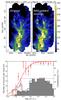 |
Fig. 10 Example of completeness analysis in the case of G202.02+2.85. Upper panel: surface brightness map of G202.02+2.85 in the 250 μm band for the true observations (left) and after adding isothermal Bonnor-Ebert sources (right). Lower panel: the black line histogram shows the mass spectrum of the added Bonnor-Ebert sources. The grey histogram represents the mass spectrum of the sources detected by getsources. The red points are the bin-by-bin ratio of the two histograms with statistical error bars defined by 1/ |

Our set of fields is diverse in terms of galactic position, galactic environment, and morphology. Completeness of our extractions is therefore expected to vary significantly from field to field. In Appendix C, we investigate the impact of distance on completeness. We show that in addition to the well-known bias on mass estimates, source temperature can also be biased towards higher values for distances greater than ~1 kpc.
In this section, we evaluate completeness for each field. In addition to distance, the morphology of the cloud and the presence of other objects along the line of sight also contribute to confusion. These characteristics vary from field to field, so we estimate the completeness field by field.
To estimate completeness, we injected simulated sources with known characteristics in the observed brightness maps of the 250, 350, and 500 μm bands. The new sources were considered critical isothermal Bonnor-Ebert spheres (BES, Bonnor 1956), and they were located at random positions following a probability distribution weighted by the column density map presented in Sect. 3.4. The mass and temperature of BES were set randomly as follows. For each field, masses were set using a log-normal distribution with the same properties as the mass function measured in the field, and completed with a flat distribution for low masses to enable measuring the completeness of the low-mass tail. An input mass distribution is shown in Fig. 10 on the example of G202.02+2.85. A normal distribution was used for temperatures with a mean temperature of 12 K and a standard deviation of 1.0 K. The contribution of each BES to the surface brightness was computed assuming a modified black-body emission with fixed spectral index β = 2, in the optically thin approximation. The upper panel of Fig. 10 compares the original SPIRE 250 μm map and the corresponding map with injected BES on the example of G202.02+2.85.
We extracted the sources using the same procedure as described in Sect. 4.1 and determined their masses as in Sect. 4.2. Completeness is then defined for each mass bin as the number of detected sources divided by the number of injected sources (see Fig. 10). Completeness was then modelled using the function f(M) = 0.5 × [ 1 + tanh(1.1(M−M50)/(M90−M50)) ], where M is the mass of the source and Mx is the mass for which f(Mx) = x%. This fit corresponds to the red solid line in Fig. 10. The masses M50 and M90 are obtained from the fit and their values are listed in Table 1. We find that distance has a stronger impact than morphology on the values of completeness. Typically, we find 90% completeness from ~0.1 M⊙ in nearby fields (≲500 pc) up to several M⊙ in the most distant fields. This wide range of completeness implies that sources from different fields cannot be compared directly. Hence, in the next sections, we have to take distance into account when discussing the statistical physical properties of our sources.
5. Statistical physical properties of cold sources
Using the catalogue presented in the previous section, in this section we examine the statistics of the source properties.
5.1. Source samples
In the following, we compare the properties of various samples of sources from our catalogue. We define here those samples. The 221 sources flagged as extragalactic are excluded from the analysis, so our largest sample is the complete catalogue of galactic sources, which contains 4245 sources. We are interested in the comparison between starless sources (1397) and sources associated with young stellar objects (538). Therefore, we make use of the classification proposed in Sect. 4.4, where flags [1] and [2] indicate that the classification derives from one or two independent methods, respectively. We also separate small sources, which are a proxy for individual (potentially prestellar) cores (2966 sources), from large sources that will be referred to as clumps (1144 sources). The definitions of cores and clumps, based on the physical sizes for these categories, are discussed in Sect. 5.2.
We use these samples mainly in Sects. 5.3 and 5.8 where distance has a limited impact. For the rest of the analysis, we select smaller samples where we keep only sources which belong to clouds with distance quality flags equal to 1 or 2 (reliable distances, see Sect. 3.1.4). Therefore, in the other parts of Sect. 5, we present our results mainly for only the 3451 galactic sources which include 2454 cores and 954 clumps (defined in Sect. 5.2), or 444 protostellar, 1191 starless, and 1816 undetermined sources.
The number of sources for each sample and the overlap between the various samples are summarised in Table 3.
5.2. Size and shape
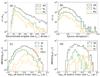 |
Fig. 11 a) Distributions of the angular deconvolved sizes of all galactic sources with distance flags [1] or [2]. The black histogram is for all galactic sources (All), green for starless sources (SL), and orange for protostellar sources (PS, flags [1] and [2]). b) Distribution of the elongation of galactic sources. c) Distributions of the linear deconvolved sizes of galactic sources. The dashed histogram is for protostellar sources with a classification flag of [2]. d) Same as frame c) after selecting sources with angular sizes larger than 60′′ for both major and minor axes. The vertical dashed lines show the size of 0.2 pc. |
For each source we computed the angular deconvolved size θdec defined as the geometric mean of the deconvolved minor and major angular FWHM sizes: θdec = (θd,majθd,min)1/2, where θd = (θmeas2−θbeam2)1/2, and θmeas is the measured FWHM of the source. The beam size θbeam = 38.5″ for all the bands because of the convolution of the maps used in the getsources analysis. The minor and major angular FWHM sizes are given by getsources for each band separately, but they vary from band to band only by a few percentage points. We chose to use the values from the column density extraction. Figure 11a shows the distribution of θdec for our full catalogue of galactic sources. It is strongly dominated by the smaller sources, peaking around 28′′. Because the spatial resolution was limited, in all likelihood we overestimated the real source sizes.
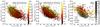 |
Fig. 12 Mean column density − dust colour temperature diagrams for the galactic sources of our catalogue with distance flags 1 or 2. The colour scale indicates the mean particle density of sources in frame a), and the source submillimetre luminosity in frame b). Frame c) compares the location of protostellar sources (points) to starless sources (grey scale). The grey scale is the starless source density in the diagram, i.e. the number of sources per bin of temperature and column density. Orange triangles: protostellar sources with flag [1] from method A (tip-down) or B (tip-up). Red diamonds: protostellar sources from both methods (flag [2]). Blue circles: protostellar sources with AKARI 65 μm counterpart. The bin-averaged temperature curves for starless and protostellar sources are over-plotted in green and orange, respectively. The vertical bars are the standard deviations for each bin-average. The black contour contains ~75% of the sources shown in frame a), and is repeated in each frame to facilitate the comparison. |
The source elongation, defined as ϵ = θmaj/θmin, is shown in Fig. 11b for the same sample. We find very similar values as previously reported by Enoch et al. (2008) for Perseus, Serpens, and Ophiuchus, i.e. a peak value of ≈1.3 and no significant differences between the starless and protostellar populations. No significant variation with the distance or with any other parameter was found.
From θdec and the distance of the cloud, we derive the linear deconvolved size Ldec for the 4110 galactic sources with distance estimates. Figure 11c shows the distribution of Ldec for all galactic sources with a distance flag of 1 or 2. It is slightly asymmetrical and peaks around 0.1 pc, a value compatible with the size of individual prestellar cores. However, ~1000 sources among the ~3400 have sizes larger than 0.2 pc and are most likely unresolved large clumps which may contain one or several individual cores. Indeed, 80% of these large sources are observed at distances ≳1 kpc, where a beam of 40′′ corresponds to ≈0.2 pc.
A significant shift is observed between the Ldec distributions of starless and protostellar sources, starless sources being apparently smaller than protostellar ones (both flags), on average. However, this result is likely to be biased because larger sources may contain several cores. Frame (d) of Fig. 11 shows the distribution of Ldec for sources with observed FWHM larger than 60′′, which are likely to be spatially resolved by a 40′′ beam. In this figure, protostellar sources seem to peak at larger sizes (0.3−0.5 pc), but the number of resolved protostellar sources is too small to draw firm conclusions. This could also be an effect of distance, because protostellar sources are detected at greater distances, on average. The fraction of sources with undetermined states of evolution increases quickly for larger sizes, suggesting that many of them are actually protostellar. Starless sources have a sharper peak around 0.1 pc with 75% of sources smaller than 0.2 pc, indicating that this population is very likely dominated by individual cores. Based on these observations, we decided to divide our catalogue into two sets of sources: cores and clumps. For the following, we define cores as sources with a deconvolved linear size Ldec< 0.2 pc (2966 sources for all distance flags, 2554 sources with distance flags of 1 or 2), and refer to sources with Ldec> 0.2 pc as clumps (1144 sources for all distance flags, 954 sources with distance flags of 1 or 2). These definitions do not take into account whether the sources are actually prestellar, and are intended to identify which sources are most likely individual sources (cores) or composed of several cores (clumps). In Sect. 5.5 we analyse whether the sources are gravitationally bound.
5.3. Source densities and temperatures
The dust colour temperature derived from SED fitting (Sect. 4.2) spans a wide range of values between 7 and 25 K; 90% of the set of galactic sources are in the range 9.9−16.9 K and have a median temperature of 12.7 K. Source temperatures are often well below the 0.1% percentile temperature T0.1% of the corresponding field given in Sect. 3.3 because aperture photometry enables the warmer contribution of background emission to be removed and therefore provides more reliable temperature estimates than T0.1%. Figure 12 shows for the full galactic sample that temperature is anti-correlated with the derived mean column density of sources, which spans several orders of magnitude with 90% of sources between N(H2) = 4.3 × 10²⁰ and 1.9 × 1022 cm-2 and a median at N(H2) = 2.2 × 1021 cm-2. These values of column density are relatively low and widely scattered compared, for example, to results reported by Enoch et al. (2008) in the case of Perseus, Serpens, and Ophiuchus (⟨ N(H2) ⟩ ≈ 1022 cm-2). The narrower scatter in the work by Enoch et al. (2008) comes from their assumption of a fixed temperature of 10 K for all their sources. The same approach applied to our data also leads to a narrow column density distribution centred around ⟨ N(H2) ⟩ ≈ 5 × 1021 cm-2. In addition, we do not use the same value for the dust opacity. Our value corresponds to κ(1.1mm) = 0.0074 cm2/g, whereas Enoch et al. (2008) use κ(1.1mm) = 0.0114 cm2/g. Using this latter value, we get masses that are smaller by a factor of 1.5, so that our different choice of the κ value tends to compensate for the effect of the fixed temperature assumption. The use of multiple submillimetre wavelengths is therefore crucial for determining both temperature and column density.
We tested the influence of distance on these diagrams by selecting subsamples in a range of distances. We find a very weak effect, mostly a slight shift towards higher dust temperatures with increasing distance, consistent with the analysis in Appendix C.
The temperature − column density distributions of sources classified as cores (Ldec< 0.2 pc) and clumps (Ldec> 0.2 pc) are very similar to the distribution for all sources, except that cores tend to fall closer to the regions with low temperature and low column density (bottom left part of the temperature − column density diagram) than clumps do. This corresponds to the region of lower bolometric luminosity in the diagram (Fig. 12b), and is consistent with the clump population corresponding to greater distances and therefore being less complete for low luminosities.
We calculated the mean particle density nFWHM of sources using the formula adapted from Enoch et al. (2008), ![\begin{equation} \label{eq:nFWHM_def} n_{\text{FWHM}} = \frac{3 M}{4\pi [d \times \langle\textit{FWHM}\rangle/2]^3 \mu m_{\text{H}}} , \end{equation}](/articles/aa/full_html/2015/12/aa24063-14/aa24063-14-eq798.png) (5)where M is the mass of the source derived from the SED of the source as presented in Sect. 4.2, d is the distance of the source,
(5)where M is the mass of the source derived from the SED of the source as presented in Sect. 4.2, d is the distance of the source,  is the geometric average of the source deconvolved size, μ = 2.33 is the mean particle mass, and mH is the proton mass. For the full galactic catalogue, we find values which cover a wide range from ~9 × 10² to ~7 × 105 cm-3 with a median around 2 × 104 cm-3. For the core population, these values are ~20% higher, whereas they are ~50% lower for the clump population. The mean density nFWHM correlates with column density and anti-correlates with temperature (Fig. 12a). The anti-correlation of densities with temperature is consistent with colder cores being more dense. However, a selection effect could also play a role, because for a similar submillimetre emission power, colder sources must have a higher column density than warmer sources. The temperature − column density relation follows lines of constant submillimetre luminosity (Fig. 12b), which supports this second interpretation.
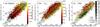 |
Fig. 13 Mass–size diagrams for the galactic sources of our catalogue with distance flags 1 or 2. The masses are derived as explained in Sect. 4.2 and the sizes are the deconvolved linear sizes derived from the getsources output for the column density map. As a comparison, the pale green band and white lines show the correlation observed for CO clumps (Elmegreen & Falgarone 1996). The two solid black lines indicate the loci for critical isothermal Bonnor-Ebert spheres at T = 7 K (lower line) and T = 20 K (upper line). The colour scale indicates the distance of sources in frame a), and the dust colour temperature of sources in frame b). Frame c) compares the location of protostellar sources (points) to starless sources (grey scale). Orange triangles: protostellar sources with flag [1] from method A (tip-down) or B (tip-up). Red diamonds: protostellar sources from both methods (flag [2]). Blue circles: protostellar sources with AKARI 65 μm counterpart. The bin-averaged mass curves for starless and protostellar sources are overplotted in green and orange, respectively. The vertical bars are the standard deviations for each bin average. |
Figure 12c compares the distributions of starless and protostellar sources. We note that for protostellar sources, the whole range of temperatures is spanned including temperatures around 10 K despite the potential presence of a YSO (see Sect. 4.4 and Fig. 7). Starless sources show the same trends as the whole catalogue. In contrast, protostellar candidates are more common than starless sources in the region with high temperature and high column density of the temperature-column density diagram. This corresponds to high bolometric luminosity, consistent with protostellar sources being more advanced than starless cores in their collapse process. For the most reliable protostellar sources (flag [2]) this trend is even more pronounced; only four sources are below the average location of starless sources (green step line in Fig. 12c). Interestingly, protostellar sources with an AKARI 65 μm counterpart (the PS[A65] group, see Sect. 4.4.2) are those with the most obvious shift compared to starless sources, suggesting that our classification is more robust for this category of protostellar sources.
5.4. The mass−size distribution
Figure 13 shows the mass–size diagram of all galactic sources with a distance flag of 1 or 2. The masses were derived as explained in Sect. 4.2. The sizes are the linear sizes from the column density maps derived from the angular deconvolved source size θdec and field distance (see Sect. 5.2).
The sources are distributed mostly along or near the correlation band reported by Elmegreen & Falgarone (1996) for CO clumps, for which mass and radius are related according to  . However, the positions of sources within the diagram are heavily affected by the adopted distance, as size and mass are proportional to the distance and its square respectively.
Dust colour temperature Tdust also correlates with source position in this diagram. The hottest sources lay below the CO clump band, i.e. in the region of extended and low-mass sources. These sources are unlikely to be gravitationally bound. When Tdust decreases, sources move towards the high-mass, small-size region of the diagram, along a direction orthogonal to the CO clump band. Only sources with Tdust ≲ 10 K fall in the region of critical isothermal Bonnor-Ebert spheres with gas temperature between T = 7 K and T = 20 K.
Starless and protostellar populations show two different behaviours. In Fig. 13c, starless sources follow the trend of CO clumps for all sizes and masses, like most sources. Protostellar sources are dominated by large and massive sources (Ldec ≳ 0.1 pc, M ≳ 3 M⊙). We note that in this diagram, as in the density-dust temperature diagram, the trend for protostellar sources is already significant when including all protostellar sources, but is more pronounced when limited to sources with the best classification flag of [2]. Again, protostellar sources from the PS[A65] group (Sect. 4.4.2) are those which exhibit the most obvious shift with respect to starless sources, here towards the high-mass part of the diagram. These values correspond to the unstable part of the diagram, beyond the critical Bonnor-Ebert sphere relation MBE ∝ BBE. Similar results were reported by Enoch et al. (2008) in the case of the Perseus cloud, but the same authors did not find a similar trend in the Serpens and Ophiucus clouds. Indeed, this general trend is difficult to observe in our individual fields, but is revealed when cumulating the sources of several clouds. This trend is consistent with the scenario discussed by Enoch et al. (2008), in which protostellar cores result from the contraction at constant mass of starless cores (horizontal shift in the mass–size diagram). It can also support the scenario described by Myers (2013), where cores are created by gravitational contraction of filaments, and experience a mass increase during their contraction, until being dispersed or forming a protostar (vertical or diagonal shift in the mass–size diagram).
5.5. Are sources gravitationally bound?
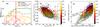 |
Fig. 14 Stability of sources as measured from the mass ratio αBE. Only sources classified as cores and with distance flags 1 or 2 are shown. a) Starless (green) vs. protostellar (orange hatched) cores for all distances (solid lines) and for distance estimates between 500 and 800 pc (dashed lines). The vertical red line indicates the αBE = 2 position. b)αBE is colour coded and represented against N(H2) and Tdust, as in Fig. 12. The black contour is repeated from Fig. 12. c)αBE is colour coded and represented against cores mass and deconvolved linear size. The blue contour shows the loci of cores with distance estimates between 500 and 800 pc. As a comparison, the pale green band and white lines show the correlation observed for CO clumps (Elmegreen & Falgarone 1996). The red lines in frames b) and c) show the αBE = 2 contours. |
For a cold core to be able to eventually form a star, it needs to be gravitationally bound. In principle, to identify gravitationally bound sources one needs to compute the virial mass from spectroscopic observations. Molecular follow-up observations of Herschel Galactic Cold Cores sources will provide this information for a number of sources, but they are not completed yet (Ristorcelli et al., in prep.; Montillaud et al., in prep.). Nevertheless, it is already possible to make a first diagnostic using the present dust observations following, for example, Könyves et al. (2010). For sources classified as cores, we computed the critical Bonnor-Ebert (BE) mass  where the BE radius RBE is taken as the observed radius
  with θd,min and θd,max the FWHM of the deconvolved minor and major axis of the source, respectively. The isothermal sound speed a is computed assuming a gas temperature of 10 K and G is the gravitational constant. We also computed the BE mass from
  , where Pext is the external pressure which we derived from the column density of the local background cloud Σcl (in g/cm-2) using the relation Pext ≈ 0.88 G Σcl2 (McKee & Tan 2003). The values of Σcl were obtained for each source individually from the source subtracted column density maps. For each source, both critical masses were computed and we calculated the BE mass ratio
 ![\hbox{$\alpha_{\rm BE} = {\rm max}[M^{\rm crit}_{\rm BE}(R_{\rm obs}), M^{\rm crit}_{\rm BE}(\Sigma_{\rm cl})]/M_{\rm obs}$}](/articles/aa/full_html/2015/12/aa24063-14/aa24063-14-eq829.png) . A value of αBE ≲ 2 is an indication of a gravitationally bound source (Könyves et al. 2010). We note that this method does not enable us to conclude whether the sources with αBE ≲ 2 are gravitationally bound and collapsing or if they are gravitationally bound and stable. Still, it makes it possible to define two groups of sources, one with αBE ≲ 2 that is likely to contain some collapsing cores and the other with αBE ≳ 2 that is unlikely to contain any collapsing cores.
. A value of αBE ≲ 2 is an indication of a gravitationally bound source (Könyves et al. 2010). We note that this method does not enable us to conclude whether the sources with αBE ≲ 2 are gravitationally bound and collapsing or if they are gravitationally bound and stable. Still, it makes it possible to define two groups of sources, one with αBE ≲ 2 that is likely to contain some collapsing cores and the other with αBE ≳ 2 that is unlikely to contain any collapsing cores.
The obtained values of αBE of cores span several orders of magnitudes and are mainly in the range 0.1−100. Figure 14a shows that the distributions of αBE for starless and protostellar cores with distance flags of 1 or 2 peak around 10 and 0.3, respectively. Only 17% of starless sources are found to be gravitationally bound, compared to 59% and 79% for protostellar sources with flags 1 and 2, respectively. This result is expected because the parent core needs to be gravitationally bound for a protostar to form. However, if a protostar is indeed present, the material detected by Herschel might be the remnant of the parent core still surrounding the protostar and is not necessarily bound. In addition, this could be related to a bias from protostellar cores being on average at greater distances, corresponding to larger physical sizes. However, the trend for αBE distributions holds when limiting the comparison to a narrow range of distances (frames a and c in Fig. 14).
We find a clear anti-correlation (r = −0.84, p-value ≪ 1%)9 between αBE and the core column density (Fig. 14b), consistent with denser cores being more likely gravitationally bound. Values of αBE ≲ 2 corresponds to column densities N(H2) ≳ 5 × 1021 cm-2. When considering the background column density instead of the source column density, we find a slightly higher threshold value of ~6 × 1021 cm-2, nevertheless with a wider scatter between ~2 and 10 × 1021 cm-2. These values are close to the threshold background column density of ~7 × 1021 cm-2 reported in Gould Belt clouds by André et al. (2014). Figure 14b also shows the variations of αBE with dust temperature. However, no correlation is found.
Figure 14c shows the mass–size diagram with αBE colour coded. We find a strong anti-correlation (r = −0.92, p-value ≪ 1%) between αBE and the core mass, and a weak anti-correlation between αBE (r = −0.60, p-value≪ 1%) and the core deconvolved linear size. Sources departing significantly from the CO clump zone towards high masses are mostly bound sources, consistent with the discussion in the previous section. A comparison with Fig. 13c shows that the locus of protostellar sources correlates well with values of αBE ≲ 2. It also shows clearly that the tail of low-mass and small-size sources most likely corresponds to small unbound and transient structures which will likely never form stars. Most of these small sources are in nearby clouds (Fig. 13a) because of higher completeness, but reciprocally we find that nearby clouds have very few bound sources, and thus are not actively forming stars. It is likely that this lack of bound sources in the close solar neighbourhood is a simple consequence of bound sources being less frequent than unbound sources. In our cloud sample, we find clouds actively forming stars for distances ≳500 pc. Sources with distances in the 500−800 pc range (blue contour in Fig. 14c) are therefore a good compromise between mass–size completeness and αBE completeness.
5.6. Core mass function
Many of our fields have too few sources to draw individual core mass function (CMF). Instead, we analyse the distribution of source masses for groups of fields. We only use the sources classified as cores in Sect. 5.2 because other sources are likely to contain several individual cores and therefore to bias the CMF towards high masses. We also restrict ouselves to the sources in clouds with reliable distance estimates (distance flags of 1 or 2). Figure 15 shows the CMF obtained for groups based on cloud distances. Only a limited effect of distance is detected up to ~300 pc. For fields with greater distances, the peak of the CMF shifts to higher masses approximately according to the square of distance. This is the same effect as in the example of the G163.82-8.44 field in Appendix C. The slope α of the high-mass tail is found to be independent of the distance. For very large distances (≳1 kpc) the scatter in α increases and prevents us from drawing conclusions for this range of distances. The value found for the majority of fields is around α(dN/ dlog (M)) = −1 (equivalent to α(dN/ dM) = −2). This is close to the values reported in other studies of potentially prestellar sources such as α(dN/ dlog (M)) = −1.3 in Perseus, Serpens, and Ophiuchus (Enoch et al. 2008), α(dN/ dlog (M)) = −1.5 in Aquila (Könyves et al. 2010), α(dN/ dlog (M)) ~ −1.35 Taurus and Orion (Sadavoy et al. 2010), and α(dN/ dlog (M)) = −1.15 and −1.20 in two fields of the Hi-GAL fields (Olmi et al. 2013). It is also similar to the values reported for the initial mass function (e.g. α(dN/ dlog (M)) = −1.3, Kroupa 2001), and the values for CO clumps α(dN/ dlog (M)) ~ −0.7 (Elmegreen & Falgarone 1996). Our values correspond to somewhat flatter high-mass tails than in other studies. This is expected because sources at different distances are included in the same CMF, which tends to flatten the resulting distribution compared to original distributions. Unfortunately, we have no way around this limitation, because further shrinking our bins of distance would result in too few sources per bin. When examining the CMF of the four clouds hosting ~100 cores or more (G155.80-14.24, G159.23-34.51, G163.82-8.44, and G271.51+5.14 with distances of 0.8 kpc, 0.325 kpc, 0.42 kpc, and 1.32 kpc, respectively), we find values typically between α(dN/ dlog (M)) = −0.5 and −1.0, in reasonable agreement with the results in Fig. 15. However, these values are very sensitive to the choice of bin width, because of the small number of sources in the high-mass tails of individual fields. In Fig. 15, thanks to the higher number of sources, the uncertainty on α due to statistical noise is only δα ~ 0.25 for the first five bins of distance, but it is important (≳1) for the two bins with distances greater than 1 kpc.
 |
Fig. 15 Core mass function (CMF) per bin of distance. The corresponding upper and lower limits of distance bins are indicated below each CMF in units of kpc. Black dashed lines are for all sources (cores + clumps), black solid lines are for all cores, and green lines for starless cores. The error bars represent the statistical error. Red vertical dashed and dotted lines show the geometrical mean of completeness at 50% and 90%, respectively (see text for details). The y-axis is set for the lower distance bin. A vertical shift by 103 was added for each next upper distance bin. The bottom right insert shows the peak positions of every CMF, defined as the peak of the best log-normal fit, as a function of the central values of distance bins. The top left insert shows the slope dN/ d(log M) of the power-law fit of the high-mass tail as a function of the central values of distance bins. In both inserts, black circles are for CMF of all sources, green squares are for starless sources. The blue solid line shows the Mpeak ∝ D2 relation. |
Beyond these limitations, we find starless sources to peak for slightly smaller masses than protostellar sources, independently of the distance. This is in contrast with the results of Olmi et al. (2013) who report slightly lower masses for protostellar objects in two Hi-GAL fields. However, our targets are much smaller in mass and less active in terms of star formation activity than the clouds analysed by Olmi et al. (2013). Our result could indicate that we detect a large fraction of transient objects and/or objects too young to form stars. Alternatively, this may be a bias in the mass estimate of protostellar sources, which are warmer than starless sources, on average. Malinen et al. (2011) showed in simulated observations that masses from submillimetre SED fitting are always underestimated, with a stronger underestimation for cold cores than for hot cores. They also showed that including PACS data, as in Olmi et al. (2013), strengthen this effect. Nevertheless, performing the same CMF analysis with temperatures derived from SPIRE + PACS 160 μm for sources observed with both instruments leads to the same shift between starless and protostellar CMFs.
We also checked the variations in the CMF with the fraction fPS of protostellar sources in the fields. We found no significant differences between fields having high and low fPS, despite the different mass functions of starless and protostellar sources in Fig. 15. This is due to the small number of identified protostellar sources compared to the sources for which we did not manage to clearly identify the stage of evolution (see Sect. 4.4).
 |
Fig. 16 Upper panel: dust temperature − mass diagram. The solid black contour contains 90% of all the sources. The grey scale shows the source surface density in the diagram for starless sources. Orange triangles: protostellar sources with flag [1] from method A (tip-down) or B (tip-up). Red diamonds: protostellar sources from both methods (flag [2]). Blue circles: protostellar sources with AKARI 65 μm counterpart. The green and orange step lines are the dust temperatures averaged over bins of the log 10 of source masses for starless and protostellar sources, respectively. The vertical bars are the reduced standard deviations for each bin-average and show that the two populations are significantly separated, on average. Lower left panel: peak position of the best log-normal fit of the reduced CMF as a function of the field-averaged source temperature. Black points are for all sources, green squares are for starless sources, and orange diamonds are for protostellar sources. Lower right panel: same as lower left panel but for the slope of the best power-law fit of the high-mass tail of the reduced CMF. |
5.7. Mass − dust temperature distribution
We used our data to look for the correlation between core mass function and core temperature. Figure 16 shows the dust temperature − mass diagram for sources with distance flags of 1 or 2 and reveals an anti-correlation between Tdust and source mass (r = −0.33, p-value ≪1%). The scatter of source characteristics is large but the trend is revealed by averaging source dust temperature within bins of source mass. The trend is confirmed when looking at the variations in CMF peak position against the field-averaged source temperature. The CMF high-mass slope α is almost constant with field-averaged source temperature ⟨ Tdust ⟩, considering the uncertainties on α, especially for protostellar sources.
The correlation between core mass function and core temperature was investigated by Sadavoy et al. (2010) in Perseus, Serpens, Ophiuchus, Taurus, and Orion. They report weak positive correlations (opposite to our results) between the CMF characteristics (peak position and high-mass tail slope) and the mean temperature of their sources. However, their results are statistically insignificant in the case of the CMF peak position (their Fig. 7a), and present large uncertainties in the case of high-mass tail slope (their Fig. 7b). Furthermore, their data did not permit a measurement of the source temperature, so they used uneven temperature estimates from previous studies, while we use a homogeneous set of data.
Figure 16 shows the results for all galactic sources, but restraining to the core population gives even stronger trends. We show in Appendix C that both masses and dust temperatures are biased towards higher values when distance increases. As a result, the trend in Fig. 16 cannot be explained by a distance-based bias; it is also underestimated because of this bias. Actually, this trend is even expected as more massive sources have more efficient self-shielding against their surrounding radiation field. On the other hand, such trends may result from a completeness issue: for a given distance, low-mass and low-temperature sources are less luminous, and therefore less complete, than higher mass and higher temperature sources.
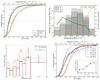 |
Fig. 17 Cumulative fraction of sources as a function of the background visual extinction. The top left frame compares starless (green) and protostellar (orange) sources. Solid lines are for all sources, dashed lines are for cores with αBE< 2. The top right frame shows, for all sources, the number of sources per bin of background column density and the mean fraction of starless (SL, green line) and protostellar (PS, orange line) sources in each bin. The bottom left frame shows the values of visual extinction AV at 50% of cumulative fraction for different bins of distance. Solid black lines are for all sources, red dashed lines for cores with αBE< 2. The bottom right frame shows the cumulative fractions for sources with αBE< 2 obtained per bin of field 9th decile temperatures T90%. The insert shows the variations in visual extinction AV at 50% of cumulative fraction as a function of T90%. The orange solid line shows Eq. (7) for β = 2, α = 4.5, and Tth = 12 K without fitting the data. The error bars in the insert and in the bottom left frame are proportional to 1/ |

In addition, we find a small shift between the positions of the starless and protostellar populations in the diagram, the latter generally falling at higher masses and warmer dust temperatures. The variations in their mass functions are similar for the peak positions up to Tdust ~ 15 K, but differ for higher Tdust and for the high-mass tail slopes, as previously mentioned. Interestingly, the trend is also correlated with the coefficient αBE. Figure 14c shows that the higher mass corresponds to more gravitationally bound sources, while Figs. 13b and 14b show that colder sources generally have lower values of αBE. Thus, the probability for source gravitational collapse is higher in the bottom right part of Fig. 16, than in the top left part.
5.8. Threshold column density effect
A threshold effect on the appearance of prestellar cores has been proposed (McKee 1989; Enoch et al. 2007, 2008; André et al. 2010; Schneider et al. 2013) according to which most prestellar cores would form in internal regions of molecular clouds surrounded by more than typically 4−8 mag of visual extinction. However, other studies either observational (Hatchell et al. 2005) or theoretical (Hennebelle & Chabrier 2011) support scenarios without a clear threshold in background density, but rather with a continuous increase in star formation rate with increasing background density. To investigate this effect in our sample of sources, we used the cumulative fraction of sources as a function of their background column density or visual extinction. We computed the background column density as described in Sect. 5.5, i.e. from getsources background maps for the column density (see Sect. 4.1). To ease the comparison with values reported in other studies, we assumed a conversion factor between column density and visual extinction H2/AV = 0.94 × 1021 cm-2 mag-1 (Bohlin et al. 1978). This value is relevant for regions with column density ≲6 × 1021 cm-2 (Draine 2003; Evans et al. 2009; Roy et al. 2014), and is therefore appropriate for the background column density of most of our sources.
The first panel of Fig. 17 shows the cumulative fractions for all galactic sources, starless sources and protostellar sources as a function of background AV. Within the sample of bound objects (αBE< 2.0), 50% of the starless sources are in regions with AV> 5 mag. For the protostellar sources the corresponding number is ~7.0 mag and thus higher by ~2 mag. This difference is consistent with denser regions being more active or more advanced in the star formation process. However, the rise of cumulative fraction is rather smooth and the notion of a single threshold does not seem quite appropriate.
The second frame of Fig. 17 compares the fraction of protostellar and starless sources as a function of background column density. In this plot, which includes all starless and protostellar sources, the proportion of protostellar sources is again seen to increase sharply with increasing background column density. This indicates that sources which lie deeper in their host cloud are more likely to be gravitationally bound and therefore to eventually form a star.
The background column densities are lower than those reported by Enoch et al. (2008), where 50% of protostellar sources of Perseus were found above cloud AV of ~12 mag and the values were even higher for Serpens and Ophiuchus. André et al. (2010), Könyves et al. (2010), and Schneider et al. (2013) reported thresholds around AV ~ 8 mag for the gravitationally bound starless cores in the Aquila Rift and in Orion. In particular, André et al. (2010) noted that in Aquila 60% of the gravitationally bound prestellar cores were found in supercritical filaments, Mline,crit> 15M⊙/pc, which corresponded to a critical value of visual extinction AV,crit. ~10 mag.
The observed differences in this study could arise from the composite nature of our sample, which contains sources from many different clouds. Mixing sources at various distances can explain partly the slow variations of our cumulative fractions because the background extinction at a cumulative fraction of 50% tends to increase with distance, however, with large fluctuations (Fig. 17).
However, when sources are divided into narrow distance bins, one can in some cases observe a similar slow rise in the cumulative fraction while in other cases the rise is steeper without a clear correlation with the distance (Fig. F.1). Therefore, if there were a single column density threshold for the appearance of gravitationally bound objects, the absence of a clear threshold in Fig. 17 cannot be fully explained by the wide range of distances in our sample.
We investigated the effect of the last decile field temperature T90% on the cumulative fractions of all galactic sources. The right panel of Fig. 17 shows the cumulative fraction obtained per 1-K bin of T90%, from 15−16 K to 19−20 K. In warmer environments, similar cumulative fractions are obtained for higher visual extinctions than in colder ones. This is in line with the idea of radiative feedback where the heating by surrounding visible-UV radiation field can prevent a core from collapsing. We propose here a very simple approach to testing more quantitatively the agreement of our data with this idea.
If a threshold (dust colour) temperature Tth exists below which cores collapse, then the visual extinction at 50% of cumulative fraction, AV(50%), can be interpreted as an indicator of the amount of matter necessary to shield the forming core from the local visible-UV radiation field surrounding the parent cloud. In the basic hypothesis of a homogeneous medium, the scaling factors of the interstellar radiation field (ISRF) XISRF and XISRF,th, respectively around the core parent cloud and within the core, can be related using XISRF,th ≈ XISRF × exp(−AV(50%)). However, it was shown that for clumpy or fractal clouds, the effective extinction can be 4 or 5 times smaller than in the homogeneous medium assumption (see e.g. Varosi & Dwek 1999), so we prefer to use XISRF,th ≈ XISRF × exp(−AV(50%) /α), where α> 1 is a constant characterising the inhomogeneity of the parent cloud. In addition, Bernard et al. (2010) proposed the following formula to relate the intensity of the local visible − UV radiation field to the dust colour temperature,  (6)where TC is the dust colour temperature, and β is the emissivity spectral index. This formula is based on a dust emission model assuming the standard dust composition proposed by Desert et al. (1990) and the spectral shape of the ISRF is similar to that of Mathis et al. (1983) for a galactocentric distance of 10 kpc, except for the integral from 0.09 to 8 μm being lower by a factor 0.81 (Bernard et al. 2010). Considering T90% as a tracer of the local visible-UV radiation field surrounding the parent cloud XISRF, and assuming that Tth similarly corresponds to XISRF,th, these two temperatures are related via AV(50%) according to
  (7)The inset in the bottom right panel of Fig. 17 compares our observational results for AV(50%) and Tth with the latter formula for β = 2, α = 4.5, and Tth = 12 K. We chose reasonable values for these parameters, without performing a fit of the data. In spite of its simplicity, this approach is in good agreement with the trend of the observations. Interestingly, the trend fully disappears for sources flagged as starless, with cumulative fractions of 50% being reached between AV = 2 and 4 for all temperatures. For sources flagged as protostellar, the trend is mostly identical to the one found with all galactic sources included although with a shift of about + 1 mag, which is consistent with the shift seen in the left panel of Fig. 17. Similar results are also obtained when limiting the analysis to bound sources (αBE< 2), however, with shifts of several magnitudes towards higher AV. This further supports the idea that the influence of the surrounding radiation field affects core collapse.
Our results suggest that if there is a column density threshold for star formation, it is not likely to be unique. Factors like the local radiation field, as well as external pressure and magnetic fields, are also likely to play a role.
6. Influence of the environment
6.1. Influence of the galactic position on core properties
Among the many parameters which may affect the properties of cold cores, we investigate here the galactic position. Large chemical gradients in the Galaxy, both in the radial and vertical directions, have been revealed by different surveys (see e.g. Fu et al. 2009; Cheng et al. 2012; Hayden et al. 2013) and are usually interpreted as the consequence of differences in chemical enrichment by various populations of stars. The average properties of molecular clouds are also known to vary systematically with galactic altitude and galactocentric distance, or according to their location relative to large structures in the Galaxy, like galactic arms or the galactic molecular ring (Honma et al. 1995; Rathborne et al. 2009; Sawada et al. 2012). We showed in Sect. 3.3 that our data also suggest variations on the scale of the Galaxy in terms of cloud dust temperature and column density. We investigated how the properties of the sources in our catalogue vary with respect to their position in the Galaxy in terms of galactocentric distance and galactic altitude. No influence of galactic altitude was found. The influence of galactocentric distance is discussed in the following subsections.
6.1.1. Median source temperature
The median source temperature ⟨ Tdust ⟩ in a field was found to decrease with the estimated galactocentric Rgal distance of the field by ~1.5 K from Rgal = 7 to 10 kpc. To assess this trend, we did a jackknife test with the following steps. For 10 000 iterations, we randomly excluded 25% of our fields. For each iteration, we computed the best linear fit to the median source temperature versus galactocentric distance of the 75% remaining fields, taking the uncertainties on Rgal due to uncertainties on distance estimates given in Table 1 into account. When including only fields with the best quality distance estimates (quality flag = 2 in Table D.1), the sample is reduced to 26 fields, most of which fall in the range Rgal = 8.0−9.2 kpc, and no trend can be derived. We therefore included all 84 fields with medium or good quality distance estimates (quality flag = 1 or 2 in Table D.1). They have Rgal in the range ~7.0−10 kpc. When including all galactic sources of our catalogue in the calculation of ⟨ Tdust ⟩, we find a significant decrease in temperature with Rgal with a slope 0.46 ± 0.17 K kpc-1 (~2.7σ). Decreasing the source sample to sources classified as clumps leads to a slope 0.47 ± 0.20 K kpc-1 (~2.3σ). A lower significance is found when only sources classified as cores (0.50 ± 0.26 K kpc-1, i.e. ~1.9σ) are selected mainly because cores generally have shorter distances. Therefore, most fields containing a significant population of cores have Rgal in the shallow range ~8−9 kpc.
Interestingly, this trend is consistent with the trend qualitatively revealed by Fig. 5 for the last decile dust temperature of the field T90% (see Sect. 3.3). In addition, ⟨ Tdust ⟩ is clearly correlated with T90%. A jackknife test similar to the one presented above provides a slope 0.58 ± 0.10 (~6σ) in the ⟨ Tdust ⟩ −T90% plane for all galactic sources, 0.69 ± 0.16 (~4σ) for clumps, and 0.57 ± 0.11 for cores (~5σ). This correlation could originate from warmer clouds forming warmer cores. However, one cannot exclude that the warmer external layers in the foreground of submillimetre sources bias the derived dust temperature towards higher temperatures.
6.1.2. Fraction of protostellar sources
The fraction of sources hosting one or several YSO candidates fYSO in each field characterises the current star formation activity of the cloud. The variations in fYSO against the galactocentric radius are V-shaped with a minimum fraction close to the Sun position Rgal, ⊙ and an increasing fraction when | Rgal−Rgal, ⊙ | increases. This is consistent with the observed correlation between fYSO and the cloud distance, for which a jackknife test gives a significance of 3.3σ, using fields with distance quality flags of 1 or 2 and all galactic sources. This can be understood as the result of the probability for the beam to intercept accidentally a mid-IR point source being proportional to the beam physical surface, which increases as the square of the (heliocentric) distance. When normalising fYSO by the squared distance, the V-shape completely disappears and a significant decrease (~3σ from jackknife test) in fYSO/D2 with increasing Rgal is found for the population of clump sources. This decrease is still present, but barely (~1.5σ) or not (0.9σ) significant when using all galactic sources or cores, respectively. This is expected because of the narrow range of Rgal covered by fields with significant numbers of cores, as mentioned in Sect. 6.1.1. It is interesting that the trend observed for clumps corresponds to an increased star formation activity in clouds having a higher T90%. A jackknife test on fYSO versus T90% gives a weak trend significant by only ~2σ.
On the other hand, it is not clear whether the trend observed for clumps traces a real increase in star formation activity for clouds having lower Rgal, because the probability for the beam to accidentally intercept a YSO should be higher when pointing to the centre of the Galaxy. As an attempt to address this question, we computed the total number of WISE point sources classified as Class I or Class II YSOs using the colour criteria of Koenig et al. (2012) in each field, and divided this number by the solid angle of the field to estimate the average YSO surface density in each field. On average, this quantity is indeed higher for fields with smaller Rgal, but the values are widely scattered and the trend is not statistically significant. When normalising fYSO with the average YSO surface density in addition to the squared distance, the correlation with Rgal is no longer significant, but it is most likely due to the additional noise introduced by the uncertainties on the normalisation factors. A better characterisation of the association between submillimetre sources and YSOs, as well as more reliable distance estimates at large distances, are required to further investigate the variations in fYSO.
6.1.3. Source mass function
In Sect. 5.6, we discussed the general properties of the core mass function in our sample of sources. We examine here the possible correlations between the variations of these general properties and the environmental conditions of clouds. We looked at the source mass function in terms of peak position and of high-mass slope, with or without completeness correction, including all sources or only sources classified as cores. No correlations with the galactic location were observed. It is unclear whether this indicates a truly universal core mass function in the Galaxy, because the analysis is hampered by distance uncertainties and variations in the completeness of source extraction.
6.2. Cloud morphology
Our fields show a variety of different morphologies, from the very simple and smooth shapes of isolated clumps found in G358.96+36.75 to the complex often filamentary structures found in G98.00+8.75. In Paper III a classification of the fields according to their morphology on the basis of a visual inspection of each field was proposed. Filaments or filamentary structures were found to be present in most fields.
We looked for correlations between the submillimetre sources and cloud morphology, as defined in Paper III, for the 71 fields presented in Paper III. Amongst the many parameters we tested are the evolutionary stage of sources (starless or protostellar), their mass, mean column density, and temperature. However, we found no significant correlation.
Similarly, no correlations were found between morphology and other cloud properties, such as the outer temperature T90% or the median column density. Notable exceptions are the correlations of morphology with cloud distance and its derived quantities like the field total mass. We find that clouds falling in the “isolated” category are usually closer than fields classified as “complex” or “filamentary and complex”. This can be expected for (i) isolated clumps, which are difficult to detect at large distances; (ii) similar field surface areas covering larger clouds at greater distances; and (iii) larger clouds, which are more likely to be sub-structured. This result illustrates the limitations of a qualitative definition of cloud morphology. In a forthcoming paper (Rivera-Ingraham et al. 2015), we propose a quantitative characterisation of the cloud morphology on the basis of filament automatic extractions using the getfilament tool (Men’shchikov 2013).
7. Conclusion
We have examined a sample of 116 fields that were mapped with the Herschel SPIRE and PACS instruments as part of the key programme Galactic cold cores. We provided distance estimates to observed clouds with uncertainties and reliability flags. Good and reasonable reliability flags were attributed to 35 and 44 clouds, respectively. These distance estimates were used to determine the positions of the clouds in the Galaxy. Most target clouds lie within ~ 1 kpc of the Sun and are part of or near well-known molecular complexes, such as the California nebula or the Orion complex. A few clouds lie at greater distances and are part of the Perseus Galactic arm. Some other clouds could be part of the Sagittarius − Carina arm. We provided dust temperature and column density maps of the observed fields. We characterised the clouds using several observables:
-
For their median column density, we found values between6 × 1019 cm-2 and 6 × 1021 cm-2 with a median value of 1.1 × 1021 cm-2. No systematic variation with the Galactic position could be found.
-
We computed the 90% percentile dust temperature T90% as a proxy for the visible-UV irradiation. Values spread between 13.7 K and 24.5 K with a median value of 16.1 K. We measured a decrease in T90% of −1.9 ± 0.6 K kpc-1 with Galactic radius, consistent with the interstellar radiation field being stronger in the inner Galaxy.
-
The total masses of the fields range from ~4 M⊙ to ~105M⊙, showing that our sample of target clouds contains objects that are very different in nature, ranging from nearby single individual cores to distant molecular complexes.
Compact sources were extracted from the maps using the multiwavelength, multiscale extraction algorithm getsources, and were analysed to build a submillimetre source catalogue containing ~4000 sources. The examination of the statistical properties of our catalogue sources and the way they relate to the characteristics of their host cloud lead to the following conclusions:
-
The extragalactic contamination of our catalogue is marginal(<5%), and the 221 potential extragalactic sources were flagged and excluded from our analysis. Therefore, our catalogue is dominated by galactic cold cores and clumps within or near star forming regions. About 65% of the sources have a deconvolved diameter smaller than 0.2 pc, compatible with an individual prestellar core. This fraction is limited by the resolution of the maps used in this study.
-
Starless and protostellar sources were identified using two methods: submillimetre temperature profile analysis and association with mid-IR sources. We showed that even if the overall submillimetre source temperature is not sufficient to disentangle starless and protostellar sources, in many cases temperature profiles show significant increases near the source centre of protostellar sources. The identification of starless sources is more challenging. The expected drop in temperature inside starless sources is difficult to detect, possibly because the emission from the coldest layers can be missed when the longest wavelength included in the analysis is SPIRE 500 μm.
-
Differences in physical properties of starless and protostellar cores are revealed by submillimetre observations: on average, starless cores are smaller in size, colder, and less dense than protostellar cores. These trends tend to be more pronounced when considering only sources classified as protostellar by both methods. The few objects classified as protostellar sources with an AKARI 65 μm counterpart tend to depart from starless sources even more clearly than the rest of the protostellar sources.
-
We find strong correlations between the gravitationally bound character of sources and their mass and column density. Only about one-third of our sources are likely to be gravitationally bound. Most of the other two-thirds follow the same trend as CO clumps in the mass–size diagram and are likely transient structures.
-
We find very similar characteristics in our CMFs to the CMFs reported for other regions, suggesting some degree of universality of the CMF. We also find an anti-correlation between the mass and temperature of starless sources.
-
Our sample of sources does not exhibit a clear threshold in background column density for the cumulative fraction of sources. Instead, the cumulative fraction of source background visual extinction increases smoothly over several magnitudes. This behaviour holds for some subsamples of sources from narrow bins of distance, showing that this result is not a consequence of distance mixing in our sample. Instead, it suggests that either there is no threshold in background column density, or there is no universal value of this threshold, leading to large variations from cloud to cloud.
-
We find a significant impact of the cloud outer temperature on the value of the background column density cumulative fractions with an increase of ~3 mag in background AV for an increase of 4 K in the cloud outer temperature. Assuming that this temperature is a tracer of the cloud visible-UV irradiation, it indicates that sources are located deeper inside molecular clouds in regions of higher visible-UV irradiation. These results show that visible-UV irradiation can be one of the factors affecting how star formation efficiency varies with density.
-
Galactic position may have an influence on star formation through the outer temperature of the clouds. However, no correlation between source characteristics and qualitative characterisation of field morphologies could be shown.
-
The lack of accuracy and reliability of distance estimates is the main limitation of the present study. It tends to blur the statistical distributions, especially for mass and size estimates, and severely hampers the study of the variations in star formation with the location in the Galaxy.
Finally, the most striking conclusion of this analysis is the prevalence of the effects of the surrounding visible-UV radiation field; we find that these effects vary on Galactic scales and have an impact on how bound cold cores distribute within their host clouds. It suggests that star formation is not driven by the only density criteria, but results from the interplay between various physical characteristics including the intensity of the visible-UV radiation field.
PACS has been developed by a consortium of institutes led by MPE (Germany) and including UVIE (Austria); KU Leuven, CSL, IMEC (Belgium); CEA, LAM (France), MPIA (Germany), INAF-IFSI/OAA/OAP/OAT, LENS, SISSA (Italy); IAC (Spain). This development has been supported by the funding agencies BMVIT (Austria), ESA-PRODEX (Belgium), CEA/CNES (France), DLR (Germany), ASI/INAF (Italy), and CICYT/MCYT (Spain).
SPIRE has been developed by a consortium of institutes led by Cardiff University (UK) and including Univ. Lethbridge (Canada); NAOC (China); CEA, LAM (France); IFSI, Univ. Padua (Italy); IAC (Spain); Stockholm Observatory (Sweden); Imperial College London, RAL, UCL-MSSL, UKATC, Univ. Sussex (UK); and Caltech, JPL, NHSC, Univ. Colorado (USA). This development has been supported by national funding agencies: CSA (Canada); NAOC (China); CEA, CNES, CNRS (France); ASI (Italy); MCINN (Spain); SNSB (Sweden); STFC (UK); and NASA (USA).
The sources are LEDA 2516652 in G139.60-3.06, 2MASX J17465090-0434329 in G21.26+12.11, and 2MASX J05521165-0821252 in G198.58-9.10. LEDA 2516652 was classified only by visual inspection of POSS II (Weinberger et al. 1999); Despite the source type proposed in Simbad, 2MASX J17465090-0434329 was actually classified as an ambiguous classification source by (Carballo et al. 1992). All other references only quote cold cores. 2MASX J05521165-0821252 was classified by Lu et al. (1990) on the basis of IRAS colour criteria judged as not satisfying by the authors themselves and which contradict the results of WISE colour criteria by Koenig et al. (2012) (see the following paragraph and Sect. 4.4.2). In addition, the authors did not detect the object in HI using the Arecibo 305 m radio telescope.
We used the NASA General Catalog Query Engine available at http://irsa.ipac.caltech.edu/applications/Gator/ to access the WISE PSC.
Acknowledgments
We warmly thank A. Mensh’chikov for his kind and efficient help in using getsources. This research made use of the SIMBAD database, operated at the CDS, Strasbourg, France. This research made use of Montage, funded by the National Aeronautics and Space Administration’s Earth Science Technology Office, Computational Technologies Project, under Cooperative Agreement Number NCC5-626 between NASA and the California Institute of Technology. The code is maintained by the NASA/IPAC Infrared Science Archive. We acknowledge the use of NASA’s Skyview facility (http://skyview.gsfc.nasa.gov) located at NASA Goddard Space Flight Center. J.Mo., M.J., and J.Ma. acknowledge the support of the Academy of Finland grant No. 250741.
References
- Alves, F. O., & Franco, G. A. P. 2007, A&A, 470, 597 [NASA ADS] [CrossRef] [EDP Sciences] [Google Scholar]
- Andersson, B.-G., Idzi, R., Uomoto, A., et al. 2002, ApJ, 124, 2164 [Google Scholar]
- André, P., Men’shchikov, A., Bontemps, S., et al. 2010, A&A, 518, L102 [NASA ADS] [CrossRef] [EDP Sciences] [Google Scholar]
- André, P., Di Francesco, J., Ward-Thompson, D., et al. 2014, Protostars and Planets VI, 27 [Google Scholar]
- Aveni, A. F., & Hunter, J. H. 1969, AJ, 74, 1021 [NASA ADS] [CrossRef] [Google Scholar]
- Bally, J., & Scoville, N. Z. 1980, ApJ, 239, 121 [NASA ADS] [CrossRef] [Google Scholar]
- Beckwith, S. V. W., Sargent, A. I., Chini, R. S., & Guesten, R. 1990, AJ, 99, 924 [NASA ADS] [CrossRef] [Google Scholar]
- Benson, P. J., & Myers, P. C. 1989, ApJS, 71, 89 [NASA ADS] [CrossRef] [Google Scholar]
- Bernard, J.-P., Paradis, D., Marshall, D. J., et al. 2010, A&A, 518, L88 [NASA ADS] [CrossRef] [EDP Sciences] [Google Scholar]
- Bohlin, R. C., Savage, B. D., & Drake, J. F. 1978, ApJ, 224, 132 [NASA ADS] [CrossRef] [Google Scholar]
- Bohnenstengel, H.-D., & Wendker, H. J. 1976, A&A, 52, 23 [NASA ADS] [Google Scholar]
- Bonnor, W. B. 1956, MNRAS, 116, 351 [CrossRef] [Google Scholar]
- Bontemps, S., André, P., Könyves, V., et al. 2010, A&A, 518, L85 [NASA ADS] [CrossRef] [EDP Sciences] [Google Scholar]
- Boulanger, F., Abergel, A., Bernard, J.-P., et al. 1996, A&A, 312, 256 [NASA ADS] [Google Scholar]
- Brunthaler, A., Reid, M. J., Menten, K. M., et al. 2011, Astron. Nachr., 332, 461 [NASA ADS] [CrossRef] [Google Scholar]
- Burton, W. B., Braun, R., & Chengalur, J. N. 2001, A&A, 369, 616 [NASA ADS] [CrossRef] [EDP Sciences] [Google Scholar]
- Carballo, R., Wesselius, P. R., & Whittet, D. C. B. 1992, A&A, 262, 106 [NASA ADS] [Google Scholar]
- Cernis, K., & Straizys, V. 1992, Balt. Astron., 1, 163 [Google Scholar]
- Cersosimo, J. C., Muller, R. J., Figueroa Vélez, S., et al. 2007, ApJ, 656, 248 [NASA ADS] [CrossRef] [Google Scholar]
- Cheng, J. Y., Rockosi, C. M., Morrison, H. L., et al. 2012, ApJ, 746, 149 [NASA ADS] [CrossRef] [Google Scholar]
- Choi, Y. K., Hachisuka, K., Reid, M. J., et al. 2014, ApJ, 790, 99 [NASA ADS] [CrossRef] [Google Scholar]
- Clemens, D. P. 1985, ApJ, 295, 422 [NASA ADS] [CrossRef] [Google Scholar]
- Clemens, D. P., Sanders, D. B., & Scoville, N. Z. 1988, ApJ, 327, 139 [NASA ADS] [CrossRef] [Google Scholar]
- Corradi, W. J. B., Franco, G. A. P., & Knude, J. 1997, A&A, 326, 1215 [NASA ADS] [Google Scholar]
- Crampton, D., & Redman, R. O. 1974, in BAAS, 6, 345 [Google Scholar]
- Cutri, R. M., Wright, E. L., Conrow, T., et al. 2011, Explanatory Supplement to the WISE Preliminary Data Release Products, Tech. Rep. [Google Scholar]
- Daddi, E., Elbaz, D., Walter, F., et al. 2010, ApJ, 714, L118 [Google Scholar]
- Dame, T. M., & Thaddeus, P. 1985, ApJ, 297, 751 [NASA ADS] [CrossRef] [Google Scholar]
- Dame, T. M., Hartmann, D., & Thaddeus, P. 2001, ApJ, 547, 792 [NASA ADS] [CrossRef] [Google Scholar]
- Desert, F.-X., Boulanger, F., & Puget, J. L. 1990, A&A, 237, 215 [NASA ADS] [Google Scholar]
- Dobashi, K., Bernard, J.-P., Yonekura, Y., & Fukui, Y. 1994, ApJS, 95, 419 [NASA ADS] [CrossRef] [Google Scholar]
- Draine, B. T. 2003, ARA&A, 41, 241 [NASA ADS] [CrossRef] [Google Scholar]
- Dunham, M. K., Rosolowsky, E., Evans, II, N. J., Cyganowski, C., & Urquhart, J. S. 2011, ApJ, 741, 110 [NASA ADS] [CrossRef] [Google Scholar]
- Dunham, M. K., Rosolowsky, E., Evans, II, N. J., et al. 2010, ApJ, 717, 1157 [NASA ADS] [CrossRef] [Google Scholar]
- Dutra, C. M., & Bica, E. 2002, A&A, 383, 631 [NASA ADS] [CrossRef] [EDP Sciences] [Google Scholar]
- Efremov, Y. N. 2011, Astron. Rep., 55, 108 [NASA ADS] [CrossRef] [Google Scholar]
- Ellsworth-Bowers, T. P., Glenn, J., Rosolowsky, E., et al. 2013, ApJ, 770, 39 [NASA ADS] [CrossRef] [Google Scholar]
- Ellsworth-Bowers, T. P., Rosolowsky, E., Glenn, J., et al. 2015, ApJ, 799, 29 [NASA ADS] [CrossRef] [Google Scholar]
- Elmegreen, B. G., & Falgarone, E. 1996, ApJ, 471, 816 [NASA ADS] [CrossRef] [Google Scholar]
- Enoch, M. L., Glenn, J., Evans, II, N. J., et al. 2007, ApJ, 666, 982 [NASA ADS] [CrossRef] [Google Scholar]
- Enoch, M., Evans II, N., Sargent, A., et al. 2008, ApJ, 684, 1240 [NASA ADS] [CrossRef] [Google Scholar]
- Evans, N. J., Dunham, M. M., Jørgensen, J. K., et al. 2009, ApJS, 181, 321 [NASA ADS] [CrossRef] [Google Scholar]
- Federrath, C. 2013, MNRAS [Google Scholar]
- Federrath, C., & Klessen, R. S. 2012, ApJ, 761, 156 [NASA ADS] [CrossRef] [Google Scholar]
- Felli, M., Palagi, F., & Tofani, G. 1992, A&A, 255, 293 [NASA ADS] [Google Scholar]
- Fischer, J., Rickard, L. J., & Stark, A. A. 1987, BAAS, 19, 726 [NASA ADS] [Google Scholar]
- Foster, J. B., Stead, J. J., Benjamin, R. A., Hoare, M. G., & Jackson, J. M. 2012, ApJ, 751, 157 [NASA ADS] [CrossRef] [Google Scholar]
- Franco, G. A. P. 1989, A&A, 223, 313 [NASA ADS] [Google Scholar]
- Fu, J., Hou, J. L., Yin, J., & Chang, R. X. 2009, ApJ, 696, 668 [NASA ADS] [CrossRef] [Google Scholar]
- Fukui, Y., Iwata, T., Mizuno, A., Bally, J., & Lane, A. P. 1993, 603 [Google Scholar]
- Glenn, J., Conley, A., Béthermin, M., et al. 2010, MNRAS, 409, 109 [NASA ADS] [CrossRef] [Google Scholar]
- Griffin, M. J., Abergel, A., Abreu, A., et al. 2010, A&A, 518, L3 [Google Scholar]
- Gutermuth, R. A., Bourke, T. L., Allen, L. E., et al. 2008, ApJ, 673, L151 [NASA ADS] [CrossRef] [Google Scholar]
- Hatchell, J., Richer, J. S., Fuller, G. A., et al. 2005, A&A, 440, 151 [NASA ADS] [CrossRef] [EDP Sciences] [Google Scholar]
- Hayden, M. R., Holtzman, J. A., Majewski, S. R., et al. 2013, AAS Meeting, 221, 254.14 [Google Scholar]
- Hearty, T., Fernàndez, M., Alcalá, J. M., Covino, E., & Neuhäuser, R. 2000, A&A, 357, 681 [NASA ADS] [Google Scholar]
- Heithausen, A., & Böttner, C. 2010, A&A, 521, L58 [NASA ADS] [CrossRef] [EDP Sciences] [Google Scholar]
- Heithausen, A., Stacy, J. G., de Vries, H. W., Mebold, U., & Thaddeus, P. 1993, A&A, 268, 265 [NASA ADS] [Google Scholar]
- Hennebelle, P., & Chabrier, G. 2011, ApJ, 743, L29 [NASA ADS] [CrossRef] [Google Scholar]
- Hennebelle, P., Commerçon, B., Joos, M., et al. 2011, A&A, 528, A72 [NASA ADS] [CrossRef] [EDP Sciences] [Google Scholar]
- Heyer, M. H., Carpenter, J. M., & Ladd, E. F. 1996, ApJ, 463, 630 [NASA ADS] [CrossRef] [Google Scholar]
- Hilton, J., & Lahulla, J. F. 1995, A&AS, 113, 325 [NASA ADS] [Google Scholar]
- Honma, M., Sofue, Y., & Arimoto, N. 1995, A&A, 304, 1 [NASA ADS] [Google Scholar]
- Hou, L. G., & Han, J. L. 2014, A&A, 569, A125 [NASA ADS] [CrossRef] [EDP Sciences] [Google Scholar]
- Hughes, J., Hartigan, P., & Clampitt, L. 1993, ApJ, 105, 571 [Google Scholar]
- Juvela, M., Ristorcelli, I., Montier, L. A., et al. 2010, A&A, 518, L93 [NASA ADS] [CrossRef] [EDP Sciences] [Google Scholar]
- Juvela, M., Ristorcelli, I., Pelkonen, V.-M., et al. 2011, A&A, 527, A111 [NASA ADS] [CrossRef] [EDP Sciences] [Google Scholar]
- Juvela, M., Ristorcelli, I., Pagani, L., et al. 2012, A&A, 541, A12 [NASA ADS] [CrossRef] [EDP Sciences] [Google Scholar]
- Kauffmann, J., Bertoldi, F., Bourke, T. L., Evans, N. J., & Lee, C. W. 2008, A&A, 487, 993 [NASA ADS] [CrossRef] [EDP Sciences] [Google Scholar]
- Kawamura, A., Onishi, T., Yonekura, Y., et al. 1998, ApJS, 117, 387 [NASA ADS] [CrossRef] [Google Scholar]
- Kennicutt, Jr., R. C. 1998, ApJ, 498, 541 [NASA ADS] [CrossRef] [Google Scholar]
- Kirsanova, M. S., Sobolev, A. M., Thomasson, M., et al. 2008, MNRAS, 388, 729 [NASA ADS] [CrossRef] [Google Scholar]
- Kiss, Z. T., Tóth, L. V., Krause, O., Kun, M., & Stickel, M. 2006, A&A, 453, 923 [NASA ADS] [CrossRef] [EDP Sciences] [Google Scholar]
- Knude, J., & Hog, E. 1998, A&A, 338, 897 [NASA ADS] [Google Scholar]
- Könyves, V., André, P., Men’shchikov, A., et al. 2010, A&A, 518, L106 [NASA ADS] [CrossRef] [EDP Sciences] [Google Scholar]
- Koenig, X. P., Leisawitz, D. T., Benford, D. J., et al. 2012, ApJ, 744, 130 [NASA ADS] [CrossRef] [Google Scholar]
- Kroupa, P. 2001, MNRAS, 322, 231 [NASA ADS] [CrossRef] [Google Scholar]
- Kun, M. 1998, ApJS, 115, 59 [NASA ADS] [CrossRef] [Google Scholar]
- Kun, M., Obayashi, A., Sato, F., et al. 1994, A&A, 292, 249 [NASA ADS] [Google Scholar]
- Kun, M., Aoyama, H., Yoshikawa, N., et al. 2001, PASJ, 53, 1063 [NASA ADS] [Google Scholar]
- Kun, M., Balog, Z., Kenyon, S. J., Mamajek, E. E., & Gutermuth, R. A. 2009, ApJS, 185, 451 [NASA ADS] [CrossRef] [Google Scholar]
- Lada, C. J., Lombardi, M., & Alves, J. F. 2009, ApJ, 703, 52 [NASA ADS] [CrossRef] [Google Scholar]
- Lada, C. J., Lombardi, M., & Alves, J. F. 2010, ApJ, 724, 687 [NASA ADS] [CrossRef] [Google Scholar]
- Lee, C. W., & Myers, P. C. 1999, ApJS, 123, 233 [NASA ADS] [CrossRef] [Google Scholar]
- Lee, Y., Snell, R. L., & Dickman, R. L. 1991, ApJ, 379, 639 [NASA ADS] [CrossRef] [Google Scholar]
- Liseau, R., Lorenzetti, D., Nisini, B., Spinoglio, L., & Moneti, A. 1992, A&A, 265, 577 [NASA ADS] [Google Scholar]
- Lombardi, M., Lada, C. J., & Alves, J. 2008a, A&A, 489, 143 [NASA ADS] [CrossRef] [EDP Sciences] [Google Scholar]
- Lombardi, M., Lada, C. J., & Alves, J. 2008b, A&A, 480, 785 [NASA ADS] [CrossRef] [EDP Sciences] [Google Scholar]
- Lombardi, M., Lada, C. J., & Alves, J. 2010, A&A, 512, A67 [NASA ADS] [CrossRef] [EDP Sciences] [Google Scholar]
- Lombardi, M., Alves, J., & Lada, C. J. 2011, A&A, 535, A16 [NASA ADS] [CrossRef] [EDP Sciences] [Google Scholar]
- Lu, N. Y., Dow, M. W., Houck, J. R., Salpeter, E. E., & Lewis, B. M. 1990, ApJ, 357, 388 [NASA ADS] [CrossRef] [Google Scholar]
- Maddalena, R. J., Morris, M., Moscowitz, J., & Thaddeus, P. 1986, ApJ, 303, 375 [NASA ADS] [CrossRef] [Google Scholar]
- Maheswar, G., & Bhatt, H. C. 2006, MNRAS, 369, 1822 [NASA ADS] [CrossRef] [Google Scholar]
- Maheswar, G., Lee, C. W., Bhatt, H. C., Mallik, S. V., & Dib, S. 2010, A&A, 509, A44 [NASA ADS] [CrossRef] [EDP Sciences] [Google Scholar]
- Malinen, J., Juvela, M., Collins, D. C., Lunttila, T., & Padoan, P. 2011, A&A, 530, A17 [CrossRef] [EDP Sciences] [Google Scholar]
- Malinen, J., Juvela, M., Zahorecz, S., et al. 2014, A&A, 563, A125 [NASA ADS] [CrossRef] [EDP Sciences] [Google Scholar]
- Marka, C., Schreyer, K., Launhardt, R., Semenov, D. A., & Henning, T. 2012, A&A, 537, A4 [NASA ADS] [CrossRef] [EDP Sciences] [Google Scholar]
- Marshall, D. J., Robin, A. C., Reylé, C., Schultheis, M., & Picaud, S. 2006, A&A, 453, 635 [NASA ADS] [CrossRef] [EDP Sciences] [Google Scholar]
- Marshall, D. J., Joncas, G., & Jones, A. P. 2009, ApJ, 706, 727 [NASA ADS] [CrossRef] [Google Scholar]
- Martin, P. G., Roy, A., Bontemps, S., et al. 2012, ApJ, 751, 28 [NASA ADS] [CrossRef] [Google Scholar]
- Mathieu, R. D. 2008, in Handbook of Star Forming Regions, Vol. I, 757 [Google Scholar]
- Mathis, J. S., Mezger, P. G., & Panagia, N. 1983, A&A, 128, 212 [NASA ADS] [Google Scholar]
- McKee, C. F. 1989, ApJ, 345, 782 [NASA ADS] [CrossRef] [Google Scholar]
- McKee, C. F., & Ostriker, E. C. 2007, ARA&A, 45, 565 [NASA ADS] [CrossRef] [Google Scholar]
- McKee, C. F., & Tan, J. C. 2003, ApJ, 585, 850 [NASA ADS] [CrossRef] [MathSciNet] [Google Scholar]
- Megeath, S. T., Allgaier, E., Young, E., et al. 2009, AJ, 137, 4072 [NASA ADS] [CrossRef] [Google Scholar]
- Men’shchikov, A. 2013, A&A, 560, A63 [NASA ADS] [CrossRef] [EDP Sciences] [Google Scholar]
- Men’shchikov, A., André, P., Didelon, P., et al. 2012, A&A, 542, A81 [NASA ADS] [CrossRef] [EDP Sciences] [Google Scholar]
- Molinari, S., Swinyard, B., Bally, J., et al. 2010, A&A, 518, L100 [NASA ADS] [CrossRef] [EDP Sciences] [Google Scholar]
- Motte, F., Zavagno, A., Bontemps, S., et al. 2010, A&A, 518, L77 [NASA ADS] [CrossRef] [EDP Sciences] [Google Scholar]
- Murakami, H., Baba, H., Barthel, P., et al. 2007, PASJ, 59, 369 [Google Scholar]
- Myers, P. C. 2013, ApJ, 764, 140 [Google Scholar]
- Nozawa, S., Mizuno, A., Teshima, Y., Ogawa, H., & Fukui, Y. 1991, ApJS, 77, 647 [NASA ADS] [CrossRef] [Google Scholar]
- Nutter, D., Ward-Thompson, D., & André, P. 2006, MNRAS, 368, 1833 [NASA ADS] [CrossRef] [Google Scholar]
- Nutter, D., Kirk, J. M., Stamatellos, D., & Ward-Thompson, D. 2008, MNRAS, 384, 755 [NASA ADS] [CrossRef] [Google Scholar]
- Nyman, L.-A., Bronfman, L., & Thaddeus, P. 1989, A&A, 216, 185 [NASA ADS] [Google Scholar]
- Odenwald, S., Fischer, J., Lockman, F. J., & Stemwedel, S. 1992, ApJ, 397, 174 [NASA ADS] [CrossRef] [Google Scholar]
- Olmi, L., Anglés-Alcázar, D., Elia, D., et al. 2013, A&A, 551, A111 [NASA ADS] [CrossRef] [EDP Sciences] [Google Scholar]
- Ossenkopf, V., & Henning, T. 1994, A&A, 291, 943 [NASA ADS] [Google Scholar]
- Otrupcek, R. E., Hartley, M., & Wang, J.-S. 2000, PASA, 17, 92 [NASA ADS] [CrossRef] [Google Scholar]
- Padoan, P., & Nordlund, A. 2011, ApJ, 730, 40 [NASA ADS] [CrossRef] [Google Scholar]
- Pagani, L., Bacmann, A., Motte, F., et al. 2004, A&A, 417, 605 [NASA ADS] [CrossRef] [EDP Sciences] [Google Scholar]
- Penprase, B. E. 1993, ApJS, 88, 433 [NASA ADS] [CrossRef] [Google Scholar]
- Pilbratt, G. L., Riedinger, J. R., Passvogel, T., et al. 2010, A&A, 518, L1 [CrossRef] [EDP Sciences] [Google Scholar]
- Planck Collaboration XXII. 2011, A&A, 536, A22 [NASA ADS] [CrossRef] [EDP Sciences] [Google Scholar]
- Planck Collaboration XXIII. 2011, A&A, 536, A23 [NASA ADS] [CrossRef] [EDP Sciences] [Google Scholar]
- Planck Collaboration XXVIII. 2015, A&A, in press, DOI: 10.1051/0004-6361/201525819 [Google Scholar]
- Plüschke, S., Cervino, M., Diehl, R., et al. 2002, New Astron. Rev., 46, 535 [NASA ADS] [CrossRef] [Google Scholar]
- Poglitsch, A., Waelkens, C., Geis, N., et al. 2010, A&A, 518, L2 [NASA ADS] [CrossRef] [EDP Sciences] [Google Scholar]
- Prato, L., Rice, E. L., & Dame, T. M. 2008, in Handbook of Star Forming Regions, Vol. I, 18 [Google Scholar]
- Racca, G. A., Vilas-Boas, J. W. S., & de la Reza, R. 2009, ApJ, 703, 1444 [NASA ADS] [CrossRef] [Google Scholar]
- Ramesh, B. 1994, JA&A, 15, 415 [Google Scholar]
- Rathborne, J. M., Johnson, A. M., Jackson, J. M., Shah, R. Y., & Simon, R. 2009, ApJS, 182, 131 [NASA ADS] [CrossRef] [Google Scholar]
- Reid, M. J., Menten, K. M., Zheng, X. W., et al. 2009, ApJ, 700, 137 [NASA ADS] [CrossRef] [Google Scholar]
- Reid, M. J., Menten, K. M., Brunthaler, A., et al. 2014, ApJ, 783, 130 [Google Scholar]
- Reipurth, B., & Gee, G. 1986, A&A, 166, 148 [NASA ADS] [Google Scholar]
- Rivera-Ingraham, A., Ristorelli. I., Juvela, M., et al. 2015, A&A, submitted [Google Scholar]
- Robin, A. C., Reylé, C., Derrière, S., & Picaud, S. 2003, A&A, 409, 523 [NASA ADS] [CrossRef] [EDP Sciences] [Google Scholar]
- Robin, A. C., Marshall, D. J., Schultheis, M., & Reylé, C. 2012, A&A, 538, A106 [NASA ADS] [CrossRef] [EDP Sciences] [Google Scholar]
- Roussel, H. 2013, PASP, 125, 1126 [Google Scholar]
- Roy, A., André, P., Palmeirim, P., et al. 2014, A&A, 562, A138 [NASA ADS] [CrossRef] [EDP Sciences] [Google Scholar]
- Sadavoy, S. I., Di Francesco, J., Bontemps, S., et al. 2010, ApJ, 710, 1247 [NASA ADS] [CrossRef] [Google Scholar]
- Saul, M., Cunningham, M., Rathborne, J., Walsh, W., & Butner, H. M. 2011, ApJ, 738, 152 [NASA ADS] [CrossRef] [Google Scholar]
- Sawada, T., Hasegawa, T., Sugimoto, M., Koda, J., & Handa, T. 2012, ApJ, 752, 118 [NASA ADS] [CrossRef] [Google Scholar]
- Schlafly, E. F., Green, G., Finkbeiner, D. P., et al. 2014, ApJ, 786, 29 [NASA ADS] [CrossRef] [Google Scholar]
- Schneider, N., André, P., Könyves, V., et al. 2013, ApJ, 766, L17 [NASA ADS] [CrossRef] [Google Scholar]
- Schwartz, P. R., Gee, G., & Huang, Y.-L. 1988, ApJ, 327, 350 [NASA ADS] [CrossRef] [Google Scholar]
- Shetty, R., Kauffmann, J., Schnee, S., & Goodman, A. A. 2009a, ApJ, 696, 676 [NASA ADS] [CrossRef] [Google Scholar]
- Shetty, R., Kauffmann, J., Schnee, S., Goodman, A. A., & Ercolano, B. 2009b, ApJ, 696, 2234 [NASA ADS] [CrossRef] [Google Scholar]
- Shetty, R., Kelly, B. C., & Bigiel, F. 2013, MNRAS, 430, 288 [NASA ADS] [CrossRef] [Google Scholar]
- Skrutskie, M. F., Cutri, R. M., Stiening, R., et al. 2006, AJ, 131, 1163 [NASA ADS] [CrossRef] [Google Scholar]
- Snell, R. L. 1981, ApJS, 45, 121 [NASA ADS] [CrossRef] [Google Scholar]
- Stark, A. A., & Brand, J. 1989, ApJ, 339, 763 [NASA ADS] [CrossRef] [Google Scholar]
- Straiẑys, V., & Laugalys, V. 2007, Balt. Astron., 16, 167 [Google Scholar]
- Sung, H., Bessell, M. S., & Lee, S.-W. 1997, AJ, 114, 2644 [NASA ADS] [CrossRef] [Google Scholar]
- Tauber, J. A., Mandolesi, N., Puget, J.-L., Banos, T., & Bersanelli, M. 2010, A&A, 520, 1 [Google Scholar]
- Tothill, N. F. H., Löhr, A., Parshley, S. C., et al. 2009, ApJS, 185, 98 [NASA ADS] [CrossRef] [Google Scholar]
- Ungerechts, H., & Thaddeus, P. 1987, ApJS, 63, 645 [NASA ADS] [CrossRef] [Google Scholar]
- Varosi, F., & Dwek, E. 1999, ArXiv e-prints [arXiv:astro-ph/9905291] [Google Scholar]
- Vilas-Boas, J. W. S., Myers, P. C., & Fuller, G. A. 1994, ApJ, 433, 96 [NASA ADS] [CrossRef] [Google Scholar]
- Wang, K., Wu, Y. F., Ran, L., Yu, W. T., & Miller, M. 2009, A&A, 507, 369 [NASA ADS] [CrossRef] [EDP Sciences] [Google Scholar]
- Weinberger, R., Gajdošik, M., & Zanin, C. 1999, A&AS, 137, 293 [NASA ADS] [CrossRef] [EDP Sciences] [Google Scholar]
- Wienen, M., Wyrowski, F., Schuller, F., et al. 2012, A&A, 544, A146 [NASA ADS] [CrossRef] [EDP Sciences] [Google Scholar]
- Wienen, M., Wyrowski, F., Menten, K. M., et al. 2015, A&A, 579, A91 [NASA ADS] [CrossRef] [EDP Sciences] [Google Scholar]
- Wilson, B. A., Dame, T. M., Masheder, M. R. W., & Thaddeus, P. 2005, A&A, 430, 523 [NASA ADS] [CrossRef] [EDP Sciences] [Google Scholar]
- Wright, E. L., Eisenhardt, P. R. M., Mainzer, A. K., et al. 2010, AJ, 140, 1868 [NASA ADS] [CrossRef] [Google Scholar]
- Wu, Y., Liu, T., Meng, F., et al. 2012, ApJ, 756, 76 [NASA ADS] [CrossRef] [Google Scholar]
- Yamamura, I., Makiuti, S., Ikeda, N., et al. 2010, AKARI/FIS All-Sky Survey Point Source Catalogues, Tech. Rep. [Google Scholar]
- Yonekura, Y., Dobashi, K., Mizuno, A., Ogawa, H., & Fukui, Y. 1997, ApJS, 110, 21 [NASA ADS] [CrossRef] [Google Scholar]
- Ysard, N., Abergel, A., Ristorcelli, I., et al. 2013, A&A, 559, A133 [NASA ADS] [CrossRef] [EDP Sciences] [Google Scholar]
- Zagury, F., Boulanger, F., & Banchet, V. 1999, A&A, 352, 645 [NASA ADS] [Google Scholar]
Appendix A: Details on source classification
In Sects. 4.4 and 4.3 we made use of ancillary data to classify our Herschel sources. On the one hand, we matched both the WISE and AKARI point source catalogues (PSC) with our Herschel catalogue. On the other hand, we made use of the colour criteria of Koenig et al. (2012) applied to the sources from the WISE PSC that match our Herschel catalogue. We provide here additional data regarding these two points.
 |
Fig. A.1 Distribution of the shift between the centre of the Herschel sources and the matching WISE sources. The black histogram and black circles show the shift distribution regardless of the classification method flag. The red histogram and red triangles show the shift distribution of sources with flag 2, i.e. classified as protostellar by methods A and B (Sect. 4.4.3). Upper panel: protostellar sources with embedded Class I and/or Class II YSOs. The scatter plot shows the correlation between the absolute and relative shifts with respect to the Herschel source size. The vertical dashed line shows the beam size. Lower panel: protostellar sources with AKARI 65 μm counterparts. Blue circles show sources classified as protostellar with embedded Class 0 YSOs. The scatter plot shows the absolute shift in WISE and AKARI source positions as a function of the absolute shift in WISE and Herschel source positions. |
Appendix A.1: Matching WISE and AKARI point source catalogues with our submillimetre catalogue
Protostellar sources with embedded Class I or Class II YSO.
In Fig. A.1, we show the histogram of the shift in position between the centre positions of WISE point sources and of our Herschel sources classified as protostellar with embedded Class I or Class II YSO. We find more than 95% of the selected WISE sources within one beam size (~40′′) of the Herschel sources. This result occurs although the size of Herschel sources is ≳40′. For the vast majority of sources, this corresponds to relative shifts below half the size of the Herschel source, computed as the geometrical average  , where θmin and θmax are the small and large FWHM of the Herschel source as determined by getsources from the column density maps.
The shifts tend to be smaller for Herschel sources classified as protostellar by both methods A and B (Sect. 4.4.3), suggesting that these sources are more reliable protostellar candidates. However, this trend could also result from the stronger distance criteria adopted in the submillimetre classification method (Sect. 4.4.1).
Overall, these results are in agreement with the idea that, for the vast majority of sources classified as Class I and/or Class II, the same source is detected at mid- and far- IR wavelengths.
Protostellar sources with embedded Class 0 YSO.
In the case of Class 0 classifications, we used both the 22 μm WISE PSC and the 65 μm AKARI PSC. We independently matched the 22 μm WISE PSC with our catalogue and the 65 μm AKARI PSC with our catalogue. We found that all sources with an AKARI 65 μm counterpart are also associated with at least one WISE 22 μm source. Figure A.1 shows that for ~65% of protostellar sources with a significant AKARI 65 μm counterpart, the shift in centre positions between the WISE and Herschel sources is less than 20′′ and also corresponds to shifts of less than 20′′ between WISE and AKARI sources. Among those sources, only ten are classified as hosts of a Class 0 YSO because the others are also associated with WISE sources classified as Class I or Class II objects. A 20′′ shift is less than the 40′′ beam of the Herschel maps used in our study, and is therefore a good match with our catalogue. The corresponding 20′′ shift between AKARI and WISE sources is more significant. The position accuracy at the 3σ level of confidence of AKARI point sources is ~6′′ (Yamamura et al. 2010), and the WISE beam at 22 μm is ~12′′, almost in agreement with the shifts observed here. Nevertheless, for the WISE PSC, Cutri et al. (2011) report astrometric accuracies below 1′′. In this case, the 20′′ shifts observed here could be significant, and may indicate that parts of the same source with different temperatures are detected at 22 μm and 65 μm. Still, the fact that a source is detected simultaneously at 22 μm and 65 μm is a strong indication of protostellar activity, while the absence of detection at shorter wavelengths suggests that the source is not evolved enough yet, hence our classification as protostellar source with embedded (potential) Class 0 YSO. This classification is strengthened by the analysis in Sect. 5 where we find that sources with a significant AKARI 65 μm counterpart (which includes our Class 0 host candidates) have distributions that depart even more clearly from starless sources than the rest of protostellar sources (Figs. 12, 13, and 16).
Appendix A.2: Colour−colour and colour−magnitude plots
In Sects. 4.4 and 4.3 we applied the colour criteria by Koenig et al. (2012) to all the sources in the WISE PSC which match
our Herschel catalogue. We show in Fig. A.2 the colour−colour and colour−magnitude plots of sources from the WISE PSC that matches our Herschel sources. The used classification criteria are those proposed by Koenig et al. (2012) in their Appendices A.1−A.3. In short, they separate Class I and Class II young stellar objects, star forming galaxies with strong PAH emission (PAH/star forming galaxy), active galactic nuclei (AGNs), unresolved knots of shock emission from outflows colliding with cold cloud material (shocks), and resolved PAH emissions.
 |
Fig. A.2 WISE colour−magnitude and colour−colour diagrams for classification of sources, showing the colour−magnitude and colour−colour criteria (black lines), AGN-classified sources (grey points with black edges), PAH/star forming galaxy-classified sources (white), shock-classified sources (yellow), resolved PAH emission-classified sources (purple), Class I-classified sources (red), Class II-classified sources (orange), and unclassified sources (small grey points without edges). |
Appendix B: Excerpt of the submillimetre source catalogue
Excerpt of a few sources from our submillimetre catalogue.
Appendix C: The effect of distance on source extraction and determination of mass and temperature
To evaluate the effect of distance on source extraction, we considered one nearby field and used it to simulate a cloud N times further (N = 2, 3, 4, 5, and 10) than the true distance. The distance of the object is modelled by convolving the Herschel maps with Gaussian beams  times wider than the beam of the instrument. Additional Gaussian random noise was added, smoothed to the beam size and scaled to ensure that the simulated maps present the same level of noise as the original images. The sources were then extracted from SPIRE maps using getsources.
We used the most extended field in our sample, G163.82-8.44, in order to have the largest possible maps for great simulated distances. This field enables us to investigate the effect of distance in the range 0.42−4.2 kpc. A stamp of the original column density map of the G163.82-8.44 field and the convolved maps for N = 3 and 10 are shown in Fig. C.1. The FWHM of the extracted sources are also plotted.
Figure C.1 shows that the structures interpreted by getsources as multiple sources in the original maps progressively merge when N increases into what getsources interprets as large single sources. As expected, this shows that the probability that compact sources extracted using getsources are actual individual
cold cores decreases very significantly with distance. We therefore pay special attention to the distance when comparing the properties of sources from different fields.
Figure C.2 shows the mass spectra of G163.82-8.44 for the original and the greater simulated distances, which we derived using the method presented in Sect. 4.2. When distance increases, the low-mass tail of mass distributions drops quickly, while the high-mass tail increases slowly because some low-mass sources are merged into bigger ones. The overall result is a regular shift in the mean core mass which varies as the square of the distance (Fig. C.2b), while the number of detected sources decreases almost proportionally to the inverse of distance. The way the slope of the high-mass tail varies with distance is less clear because this quantity is not well defined for this field and is very sensitive to the number of bins used to draw the mass distribution. Performing the same exercise on other fields leads to the same conclusions. This is also in line with the results of Malinen et al. (2011) obtained from simulated observations.
The effect of distance on dust temperature estimates is evaluated in Fig. C.2c. We do not find clear variations for N ≤ 3 (distance ≲1.5 kpc). In contrast, for greater distances, more low-temperature (Tdust ≤ 12 K) sources are missed than warmer sources. As a result, the mean dust temperature increases with distance. This effect is of particular interest for our discussion of Fig. 16 in Sect. 5.7.
 |
Fig. C.1 Left: close-up view of G163.82-8.44 centred at RA = 4h28m01.8s Dec = +36°45m51.87s. The colour scale shows the H2 column density derived from SPIRE data. The cyan ellipses show the FWHM of the sources obtained using getsources. Middle and right frames show the same field with simulated distances 3 and 10 times greater than the estimated distance of 0.42 kpc. |
 |
Fig. C.2 a) Source mass function of the G163.82-8.44 field for several values of the simulated distance. b) Number of sources (red circles) and average of the logarithm of source masses (orange squares) as functions of the simulated distance. The vertical bars show the standard deviation of the logarithm of source masses. The solid grey line shows a power law with exponent 2 on the right y-axis. Dotted and dashed lines are plotted to guide the eye. c) Histogram of dust colour temperature Tdust of G163.82-8.44 sources for several values of the simulated distance. In the inset, orange squares show the average values of Tdust and the vertical bars show the standard deviation of Tdust as functions of the simulated distance. |
Appendix D: Details on distance estimates
In Sect. 3.1, we presented all the methods used to estimate the source distances, their associated uncertainties, and reliability flags. In Table D.1, we gather all the distance estimates obtained for all the methods. We provide the radial velocities extracted from the CO data of Dame et al. (2001) and compare them with the radial velocities from Wu et al. (2012). For the extinction method, we provide the most important parameters:
-
the number of stars Nstar detected in the 5 and 10 arcmin apertures, which should be higher than ~100 to enable good statistics in the comparison of observations with the Galactic model (Marshall et al. 2009);
-
the probability
 for the model to agree with the observed star count; values above 0.2 indicate a reasonable agreement;
 -
the significance σdet of the cloud detection, i.e. the ratio between the extinction of the cloud and the diffuse extinction.
The distance estimates found in the literature are also provided, along with the corresponding references.
Data used for distance estimates.
In addition, we provide here field-by-field short justifications for the adopted distances, based on the data presented in Table D.1.
Appendix D.1: G0.02+18.02
This field is located towards the Galactic centre, so that kinematic distances are not reliable. The extinction method provided a reasonable result only for the large aperture (10′), but with a low agreement probability ( ) between 2MASS stars and the extinction model. Therefore this value should be considered as an upper limit. In addition, the cloud is likely to be associated with the Ophiuchus complex at 160 ± 50 pc (Nozawa et al. 1991), in agreement with the extinction upper limit of 160 ± 210 pc. For these reasons, we adopt a distance of 160 ± 50 pc with a reliability flag of 1.
Appendix D.2: G0.49+11.38
This field is located towards the Galactic centre, so that kinematic distances are not reliable. The extinction method provided reasonable results for both the small (5′) and large (10′) apertures, but with a low number of stars or low agreement probability ( ). Therefore these values (360 ± 390 pc and 160 ± 200 pc, respectively) should be considered as upper limits. For want of better data, we adopt a distance of
  pc with a reliability flag of 0.
Appendix D.3: G1.94+6.07
This field is located too close to the Galactic centre direction, so that kinematic distances are not reliable. The extinction method provided reasonable results for both the small (5′) and large (10′) apertures, but with low agreement probabilities . Therefore, these values (190 ± 520 pc and 300 ± 350 pc, respectively) should be considered as upper limits. In addition, the cloud is likely to be associated with the Pipe Nebula at 145 ± 16 pc (Alves & Franco 2007), in agreement with the distance upper limits provided by the extinction method. For these reasons, we adopt a distance of 145 ± 50 pc with a reliability flag of 1.
Appendix D.4: G2.83+21.91
This field is located too close to the Galactic centre direction, so that kinematic distances are not reliable. The extinction method provided a reasonable result only for the large aperture (10′), but with a low agreement probability ( ) between 2MASS stars and the extinction model. Therefore, this value should be considered as an upper limit. We note that with a galactic latitude of ~22 degrees, such a great distance would correspond to a very large and unlikely galactic height. In addition, the cloud might be associated with the Ophiuchus complex at 160 ± 50 pc (Nozawa et al. 1991), but this association requires a deeper investigation. For want of better data, we adopt a distance of 300 ± 300 pc with a reliability flag of 0.
Appendix D.5: G3.08+9.38
This field is located too close to the Galactic centre direction, so that kinematic distances are not reliable. The extinction method provided reasonable results for both the small (5′) and large (10′) apertures, but with very low agreement probabilities . Therefore these values (230 ± 300 pc and 210 ± 300 pc, respectively) should be considered as upper limits. Several references provide distance estimates that can be relevant for this cloud. The cloud might be associated with the Ophiuchus complex at 160 ± 50 pc (Nozawa et al. 1991; Dutra & Bica 2002). Reipurth & Gee (1986) provide a distance estimate to LDN100 of 225 ± 25 pc based on its association with a field star. This globule is located at the north-west edge of our Herschel field, its excited part appearing in the north-west corner of the WISE 22 μm map in Fig. G.1, while part of the external layers of the globule can be seen at the edge of the SPIRE maps in the same figure. The same globule was observed at radio wavelengths by Felli et al. (1992), who propose a similar distance of 230 pc based on a kinematic method. Looking the IRAS 100 μm data of this region suggests that our cloud is more likely associated with the molecular complex than with LDN 100. For these reasons, we adopted a distance of  pc where the error bar accounts for the uncertainty on which structure is more likely associated with our cloud. Considering the large amount of available data and their overall good agreement, we propose a reliability flag of 2 for the distance estimate and uncertainty pair.
Appendix D.6: G3.72+21.02
This field is located too close to the Galactic centre direction, so that kinematic distances are not reliable. The extinction method provided a reasonable result only for the large aperture (10′), but with a very low agreement probability ( ). Therefore this value should be considered as an upper limit, but the very large value (4.33 kpc) does not provide a strong constraint. The cloud might be associated with the Ophiuchus complex at 160 ± 50 pc (Nozawa et al. 1991), like G2.83+21.91 which is barely 1 degree westward. For want of better data, we adopt a distance of 160 ± 50 pc with a reliability flag of 0.
Appendix D.7: G4.18+35.79
This field (L134) is located too close to the Galactic centre direction, so that kinematic distances are not reliable. The (statistical) extinction method did not provide any results. However, Franco (1989) analysed the extinction towards individual stars in the same region, and propose a distance estimate of 110 ± 10 pc. Another work based on extinction measurements yields 141 ± 20 pc (Cernis & Straizys 1992). Hilton & Lahulla (1995) gathers the various estimates available, but there is no easy way to select a better estimate. In paper III, we chose the estimate by Cernis & Straizys (1992) for this field, and the one by Franco (1989) for G6.03+36.73 (L183), which is considered to be connected with G4.18+35.79 (Hilton & Lahulla 1995). Here, we prefer to make the same choice for both clouds, and we adopt 110 ± 10 pc with a reliability flag of 1.
Appendix D.8: G6.03+36.73
This field belongs to the same region as G4.18+35.79, and very similar data are available. We adopt the same estimate and its associated uncertainty, 110 ± 10 pc with a reliability flag of 1.
Appendix D.9: G9.45+18.85
This field is located too close to the Galactic centre direction, so that kinematic distances are not reliable. The extinction method provided a reasonable result only for the large aperture (10′) with reasonable characteristics (a good number of stars, reasonable probability, and significance). We adopt this value (280 ± 100 pc) for our study. However, this is the only result available, thus we adopt a reliability flag of 0.
Appendix D.10: G10.20+2.39
Radio observations of CO by Dame et al. (2001) show two different components at VLSR = 5.13 and 21.55 km s-1, suggesting that two structures overlap in the field. Considering the relatively low latitude (near the Galactic plane) and longitude (relatively near the Galactic centre) of the field, the presence of several structures seems probable. Indeed, the two velocities convert into two very different distances: ~3 kpc and ~1 kpc. The kinematic estimate of 3.110 kpc by Wang et al. (2009) is consistent with only one of the two components. The extinction method provides consistent estimates for both apertures (830 ± 810 pc and 960 ± 540 pc), even though the result for the large aperture has a very low agreement probability ( ). These two results are also in agreement with the nearest component of the CO observations. For this reason we favour the nearby component.
The uncertainty on the peculiar velocity V0 is illustrated by the two adopted values 0 and −15 km s-1. For V0 = 0 km s-1 and V0 = −15 km s-1 we find 0.52 kpc and 1.00 kpc, respectively, with very large formal uncertainties. The difference between these two values is of the same order of magnitude as the uncertainty on extinction estimates. Therefore, we adopt a distance of 830 ± 400 pc, where the uncertainty embraces the dispersion of extinction and kinematic estimates. However, this analysis does not exclude that the main component in this field could be the further one. It is also possible that both components overlap with similar levels of contribution, so that the sources of our catalogue originating from this field could lay at various distances. Therefore, we propose a reliability flag of 0.
Appendix D.11: G20.72+7.07
Kinematic distance estimates point to a ~1 kpc distance. On the other hand, the extinction method provides values of 260 pc and 130 pc for the small and large apertures, respectively. However, the very low agreement probabilities indicate that these values should be considered as upper limits. In addition, the cloud is likely associated with the Aquila Rift complex with a distance of 260 pc (Bontemps et al. 2010), rather compatible with the extinction estimates. If this association is correct, the kinematic method is not able to provide reliable results so that the difference between the kinematic and complex association methods is to be expected. For want of better data, we adopt a distance of 260 ± 260 pc with a reliability flag of 0.
Appendix D.12: G21.26+12.11
Radio observations of CO by Dame et al. (2001) and Wu et al. (2012) show three different velocities at VLSR = 3.47, 4.55 and 5.86 km s-1, which lead to many incompatible distance estimates between 0.06 and 15 kpc when assuming a peculiar velocity V0 equal to 0. In contrast, when assuming V0 = −15 km s-1, the three velocities provide rather consistent values of distance (480, 580 and 700 pc). However, the high galactic latitude of this region make the kinematic method unreliable.
The extinction method only provides a result for the large aperture, and with a low agreement probability . The value of 120 pc should therefore be considered as an upper limit. However, in Paper III, a previous version of the same method applied to a slightly different region of the same field provided an estimate of 730 pc.
For the sake of consistency, we adopt again a distance of 730 ± 730 pc, but considering the large uncertainties and inconsistencies between the various methods, we propose a reliability flag of 0.
Appendix D.13: G24.40+4.68
Radio observations of CO by Dame et al. (2001) show only one component, suggesting that the region is quite simple. The kinematic method provides estimates below 1 kpc and are therefore not reliable. The extinction method provided reasonable results for both the small (5′) and large (10′) apertures, but with a low number of stars or low agreement probability . Therefore, in principle, these values (250 pc and 100 pc, respectively) should be considered as upper limits. We note that in this field the region of high extinction is quite small so that the large aperture contains a large area with low extinction. This tends to bias the mean reddening to small values, and therefore also the distance to small values. For this reason, we trust the small aperture estimate more. In addition, the target cloud is likely to be associated with the Aquila Rift complex at a distance of 260 pc (Bontemps et al. 2010), which is compatible with the extinction estimate. Therefore, we adopt a distance of 260 ± 50 pc, and because of the clear understanding of the various values, we propose a reliability flag of 1.
Appendix D.14: G25.86+6.22
Radio observations of CO by Dame et al. (2001) show several components, suggesting that the field shows significant overlap of several structures. As it does for G21.26+12.11, the kinematic method provides many incompatible estimates when assuming a specular velocity V0 = 0 km s-1, but a more consistent set of distances between 390 and 810 pc when assuming V0 = −15 km s-1. We note that in the data by Dame et al. (2001), the brightest component has a velocity of 7.55 km s-1, which corresponds closely to the Aquila Rift typical velocities (5−10 km s-1, Prato et al. 2008).
The extinction method provided reasonable results for both the small (5′) and large (10′) apertures, but with low agreement probabilities . Therefore, these values (280 pc and 240 pc, respectively) should be considered as upper limits.
In addition, the target cloud is likely to be associated with the Aquila Rift complex at a distance of 260 pc (Bontemps et al. 2010), which is compatible with the extinction estimate. Therefore, we adopt a distance of 260 ± 50 pc, but because there might be some contribution by a fainter structure, we propose a reliability flag of only 1.
Appendix D.15: G26.34+8.65
Radio observations of CO by Dame et al. (2001) show two components at VLSR ≈ 5 and 10 km s-1, but that it is clearly dominated by the second one. All the derived kinematic distances are below 1 kpc. The extinction method provided two similar estimates of 200 and 250 pc for the small and large apertures, respectively. Both have low agreement probabilities , so these values should be understood as upper limits. However, Fig. G.3 shows that the cloud of interest in this field has a relatively small angular size (≲2′), small compared to both the 5 and 10′ apertures, meaning that the extinction estimates tend to be biased towards small distances. In Paper III, we estimated this distance to 0.96 kpc from a previous version of the extinction method of Marshall et al. (2009), and applied to a smaller region more appropriate to the cloud. Similarly, Clemens et al. (1988) provide a kinematic estimate of 1.2 kpc, using a different galactic rotation curve.
Finally, we propose a distance estimate of 1.0 ± 0.3 kpc, consistent with the distance adopted in Paper III, with a distance flag of 1. Here the uncertainty is set to embrace the difference between the estimate provided by Clemens et al. (1988) and Juvela et al. (2012).
Appendix D.16: G37.49+3.03
Radio observations of CO by Dame et al. (2001) show one component at VLSR = 13.9 km s-1, indicating that this field is a simple region. The two derived kinematic distances are 500 pc and 1.13 kpc. The extinction method provided two similar estimates of 640 and 740 pc for the small and large apertures, respectively. Both of them have low agreement probabilities , so that these values should be understood as upper limits. We found no reference relevant for this region providing a distance estimate. The cloud of interest in this field has a relatively small angular size (~0.5−1′). In addition, the brightest source at 250 μm clearly corresponds to a dark region at 22 μm. This suggests that this source is composed of resolved individual dense cores, and therefore distances much greater than ~1 kpc are unlikely. Assuming a physical diameter of ~0.2 pc for the 0.8′ cores, we derive a distance of ~800 pc. This value is in reasonable agreement with the extinction estimates considering that the source is small compared to both the 5 and 10′apertures (meaning that the extinction estimates tend to be biased towards small distances).
Finally, we propose a distance estimate of 800 ± 600 pc with a distance flag of 0.
Appendix D.17: G37.91+2.18
Radio observations of CO by Dame et al. (2001) show two components at VLSR ≈ 11 and 30 km s-1, but is clearly dominated by the second one, which intensity increases when approaching the Galactic plane (south-east direction in Fig. G.4). It is therefore likely that for this field, the stronger CO component corresponds to the strong background emission, while the fainter component corresponds to the cloud of interest appearing in the foreground with smaller scales. Interestingly, the faint component has a velocity of 11.4 km s-1, quite close to the velocity detected in the nearby field G37.49+3.03 (13.9 km s-1), for which we estimated a distance of ~800 pc. Here, from the faint component, we derive a kinematic distance of 330 pc (V0 = 0 km s-1) or 970 pc (V0 = −15 km s-1), in relative agreement with the proposed distance of G37.49+3.03. In contrast, the brighter component at 30.17 km s-1 leads to kinematic distances of 1.48 kpc (V0 = 0 km s-1) or 2.11 kpc (V0 = −15 km s-1). This is consistent with the proposed view that the stronger component corresponds to background emission. Unfortunately, the data by Dame et al. (2001) have too low spatial resolution to draw definite conclusions.
The extinction method provided two identical estimates of 1.06 kpc for the small and large apertures. The large one has a low agreement probability , but the small one has good characteristics. In this field, the dense structures are typically ~0.4′ wide, smaller than in G37.49+3.03, possibly suggesting a greater distance. This is consistent with the comparison of their extinction estimates.
Finally, we adopt the extinction estimate of 1.06 ± 0.79 kpc. We adopt a distance flag of 1 on the basis of the relative agreement between kinematic and extinction estimates.
Appendix D.18: G39.65+1.75
Radio observations of CO by Dame et al. (2001) show one component at VLSR ≈ 28 km s-1, indicating that this field shows a single structure. The two derived kinematic distances are 1.36 kpc (V0 = 0 km s-1) and 2.02 kpc (V0 = −15 km s-1). The extinction estimate (0.99 kpc) for the small aperture (5′) has very good characteristics (large enough number of stars, high value of the agreement probability ) and is in good agreement with the kinematic estimates for (V0 = 0 km s-1). However, it has a large uncertainty (0.96 pc). In Paper III, from a previous version of the extinction method of Marshall et al. (2009), the extinction estimate for a slightly different area of the same cloud led to 1.82 kpc, significantly higher than our extinction estimate, but still compatible with it when considering the uncertainty, and in good agreement with the kinematic estimates.
Therefore, we adopt a intermediate estimate of 1.5 ± 0.5 kpc, where the uncertainty is set to include the various estimates. Considering the overall good agreement, we adopt a reliability flag of 1.
Appendix D.19: G62.16-2.92
Radio observations of CO by Dame et al. (2001) show one component at VLSR ≈ 10 km s-1, indicating that this field shows a single structure. The two derived kinematic distances are 0.12 kpc (V0 = 0 km s-1) and 1.37 kpc (V0 = −15 km s-1). The extinction estimates, 1.02 kpc for the small aperture (5′), and 1.14 kpc for the large aperture (10′), are consistent and have rather good characteristics (large numbers of stars, large significance, but small agreement probabilities ). They are also in good agreement with the kinematic estimate for (V0 = −15 km s-1). In Paper III, from a previous version of the extinction method of Marshall et al. (2009), the extinction estimate for a slightly different area of the same cloud led to 1.11 kpc.
Therefore, we adopt the extinction estimate of 1.11 ± 0.35 kpc, where the uncertainty is set to include all the consistent estimates, and is consistent with the formal uncertainties provided by the extinction method. Considering the overall good agreement, we adopt a reliability flag of 1.
Appendix D.20: G69.57-1.74
Radio observations of CO by Dame et al. (2001) show components at VLSR ≈ 6 and 14 km s-1, but is dominated by the second one. Wu et al. (2012) performed dedicated CO observations towards one of the clump in this field and found VLSR ≈ 11 km s-1, in better agreement with the brighter component. The VLSR = 11 km s-1 and VLSR = 14 km s-1 lead respectively to kinematic estimates of 0.18 and 0.46 kpc for V0 = 0 km s-1 and 2.81 and 2.87 kpc for V0 = −15 km s-1.
The extinction method provided two similar estimates of 1.78 kpc and 1.54 kpc for the small and large apertures, respectively. They both have reasonable characteristics, despite low agreement probabilities . As a comparison, in Paper III, from a previous version of the extinction method of Marshall et al. (2009), the extinction estimate for a slightly different area of the same cloud led to 1.58 kpc.
Therefore, we adopt the extinction estimate of 1.78 ± 0.81 kpc, where the uncertainty is similar to the formal uncertainty given by the extinction method, and includes a fair part of the possible kinematic distances. We adopt a distance flag of 1 on the basis of the relative agreement between kinematic and extinction estimates.
Appendix D.21: G70.10-1.69
This field is very close to G69.57-1.74 and has very similar distance estimates. Following the same reasoning, we adopt the extinction estimate of 2.09 ± 0.83 kpc, where the uncertainty is similar to the formal uncertainty given by the extinction method, and includes a fair part of the possible kinematic distances. We adopt a distance flag of 1 on the basis of the relative agreement between kinematic and extinction estimates.
Appendix D.22: G71.27-11.32
This field is outside the CO data by Dame et al. (2001), and the extinction method failed producing distance estimates.
Appendix D.23: G82.65-2.00
Radio observations of CO by Dame et al. (2001) show one component at VLSR = 3.47 km s-1, indicating that this field is dominated by a single structure. The two derived kinematic distances are 3.30 kpc (V0 = 0 km s-1) and 1.08 kpc (V0 = −15 km s-1). The extinction estimates, 0.42 kpc for the small aperture (5′), and 0.98 kpc for the large aperture (10′), differ by a factor of 2. However the difference between these two values is included in the formal uncertainties provided by the method. In Paper III, from a previous version of the extinction method of Marshall et al. (2009), the extinction estimate for a slightly different area of the same cloud led to 0.89 kpc. Dobashi et al. (1994) propose a distance of 800 pc for their cloud 16 (l = 82.93, b = −2.03), but referring to the work by Bally & Scoville (1980) on the Pelican nebula (l = 84.63, b = + 0.10) who adopted a distance of 1 kpc. Examining the CO data cube (position-velocity space) by Dame et al. (2001), the Pelican nebula indeed seems to be connected with our target cloud. The more recent work by Cersosimo et al. (2007) shows that several structures are seen in the region of the Pelican nebula, corresponding to different velocity components in molecular observations. In their study, the region which is closest to our field (l = 84, b = −1.7) also has a similar velocity of +2.2 km s-1. They derive a distance of 700 ± 500 pc for this structure, and propose greater distances (1.7 kpc, 2.7 kpc and 3.3 kpc) for all other structures.
Considering the amount of data converging around ~1 kpc, we adopt a distance estimate of 1.0 ± 0.5 kpc, where the uncertainty is set to include most extinction estimates and a fair part of the possible kinematic distances with a reliability flag of 1.
Appendix D.24: G86.97-4.06
Radio observations of CO by Dame et al. (2001) show one component at VLSR = 3.35 km s-1, indicating that this field is dominated by a single structure. The two derived kinematic distances are 2.41 kpc (V0 = 0 km s-1) and 0.40 kpc (V0 = −15 km s-1). No extinction estimates could be obtained within our apertures. However, in Paper III, from a previous version of the extinction method of Marshall et al. (2009), the extinction estimate for a slightly different area of the same cloud led to 1.87 kpc.
In addition, the field is located at the edge of the Cygnus Rift, whose distance is estimated at 700 pc (Dame & Thaddeus 1985). If the observed cloud is associated with this structure, we derive a galactic height of −50 pc, which seems reasonable. For the distance of 1.87 kpc, one gets a galactic height of −133 pc, which seems less probable.
Considering the large inconsistency, we adopt a flag of 0, and assume that the cloud is associated with the Cygnus Rift (700 ± 100 pc).
Appendix D.25: G89.65-7.02
Radio observations of CO by Dame et al. (2001) show one component at VLSR = 11.57 km s-1, indicating that this field is dominated by a single structure. However, Wu et al. (2012) observed four sources in this field with velocities ~1 km s-1 higher. The derived kinematic distances are all very small, below 50 pc, which is aberrant. This is due to the proximity of the direction l = 90 deg, b = 0 deg.
In addition, extinction estimates are very inconsistent. The small aperture gives an upper limit of 160 pc, while large aperture provides a large value of 4.43 kpc. In Paper III, from a previous version of the extinction method of Marshall et al. (2009), the extinction estimate for a slightly different area of the same cloud led to an intermediate result of 1.21 kpc.
Considering the large inconsistencies, we simply adopt the same value as in Paper III, but with a reliability flag of 0. For want of better data, we adopt an uncertainty equal to the adopted distance.
Appendix D.26: G91.09-39.46
This field is outside the CO data by Dame et al. (2001), and the extinction method failed producing distance estimates. The distance estimate reported by Burton et al. (2001) is for the high velocity cloud CHVC092-39-367, located one degree apart from G91.09-39.46. There are no evidence for a potential connection between the two clouds. We do not provide any distance estimate for this cloud.
Appendix D.27: G92.04+3.93
Radio observations of CO by Dame et al. (2001) show two components at VLSR ≈ −4.1 and −12.1 km s-1, but seems dominated by the first one. Wu et al. (2012) performed dedicated CO observations towards seven clumps in or near this field and found various VLSR between −0.92 and −12 km s-1. This indicates that several structures may overlap in this field. However, the line of sight is too close to the direction l = 90 deg, b = 0 deg, and no reliable kinematic distance can be determined.
The extinction method provided only one result (800 ± 800 pc) for the large aperture (10′) with good characteristics, but with a very large uncertainty.
The cloud might be associated with the Cygnus OB7 complex with a distance of 800 pc (Plüschke et al. 2002), consistent with the extinction estimate. Therefore, we adopt a distance of 800 ± 100 pc with a reliability flag of 0.
Appendix D.28: G92.63-10.43
Wu et al. (2012) performed dedicated CO observations towards two clumps in this field and found VLSR of −0.22 and −0.77 km s-1. These are close values and suggest that the observed clumps belong to a single structure. However, no reliable kinematic distance can be derived due to the proximity of the direction l = 90 deg, b = 0 deg, and to the large galactic latitude.
The extinction method provide a good quality estimate of 1.84 ± 0.07 kpc, but only for the large aperture. Without additional data, it is difficult to assess the reliability of this estimate. Therefore we adopt this value and its uncertainty, but with a reliability flag of 0.
Appendix D.29: G93.21+9.55
Radio observations of CO by Dame et al. (2001) show one component at VLSR = −3.09 km s-1, indicating that this field is dominated by a single structure. Wu et al. (2012) observed seven sources in or near this field with velocities between −3.39 and 1.31 km s-1, where the nearest clumps have the nearest velocity to the value found with the data by Dame et al. (2001). We conclude that the field is dominated by a single structure. Kinematic distances can only be obtained for a peculiar velocity V0 = 0 km s-1. They range between 1.78 kpc and 2.46 kpc.
The extinction method failed to provide an estimate for the small aperture, and the estimate for the large aperture has a too low value of , leading to an estimate of 180 pc considered as an upper limit. However, in Paper III, from a different extinction method (McGehee, in prep.), the extinction estimate for the same cloud led to a result of 300 pc. This last value is relatively close to 440 pc, the distance of the nearby Cygnus complex (Dobashi et al. 1994). We adopt this latter value for this field with uncertainty of 200 pc and a reliability flag of 1.
Appendix D.30: G94.15+6.50
Radio observations of CO by Dame et al. (2001) show one component at VLSR = −2.56 km s-1, indicating that this field is dominated by a single structure. Kinematic distances do not provide strong constraints with values between 2.17 kpc (V0 = 0 km s-1) and 0 pc (V0 = −15 km s-1).
The extinction method provides two similar estimates of 320 pc (small aperture) and 270 pc (large aperture), however with large uncertainties. In Paper III, from a different extinction method (McGehee, in prep.), the extinction estimate for the same cloud led to a result of 250 pc. On the other hand, the field is near the Cygnus complex, and could be associated with it (800 pc, Dobashi et al. 1994). Considering that two different extinction methods converge on similar values, we favour the estimate from Paper III, however with an uncertainty equal to the adopted distance, and with a reliability flag of 0.
Appendix D.31: G95.76+8.17
Radio observations of CO by Dame et al. (2001) show one component at VLSR = −2.23 km s-1. Wu et al. (2012) performed dedicated CO observations towards two clumps in this field and found VLSR of −0.43 and 0.38 km s-1. The difference may arise because the data of Dame et al. (2001) in this region are spatially under-sampled, and because of the relatively low spectral resolution of these data. Kinematic distances do not provide strong constraints with values between 1.97 kpc (V0 = 0 km s-1) and 0 pc (V0 = −15 km s-1).
The extinction method provided only one result (210 ± 210 pc) for the large aperture (10′) with very low value of .
The cloud might be associated with the Cygnus complex with a distance of 800 pc (Dobashi et al. 1994), but this is not consistent with other estimates. For want of better data, we adopt the estimate 800 ± 100 pc with a reliability flag of 0.
Appendix D.32: G98.00+8.75
Radio observations of CO by Dame et al. (2001) show one component at VLSR = 2.55 km s-1. Wu et al. (2012) performed dedicated CO observations towards one clump in this field and found VLSR of 3.41 km s-1. The difference may arise because the data of Dame et al. (2001) in this region are spatially under-sampled, and because of the relatively low spectral resolution of these data. Kinematic distances do not provide strong constraints with values between 1.21 kpc (V0 = 0 km s-1) and 0 pc (V0 = −15 km s-1).
The extinction results have overall good characteristics (large enough numbers of stars, and either the probability or the significance is large enough). The small aperture provides 0.99 kpc, close to the estimate of 1.16 kpc from the large aperture. In Paper III, from a previous version of the extinction method of Marshall et al. (2009), the extinction estimate for a slightly different area of the same cloud led to a similar result of 1.12 kpc.
Considering the overall good agreement between kinematic and extinction values and the robustness of extinction estimates, we adopt 1.1 ± 0.3 kpc and a reliability flag of 2.
Appendix D.33: G105.57+10.39
Radio observations of CO by Dame et al. (2001) show one component at VLSR = −11.53 km s-1. Wu et al. (2012) performed dedicated CO observations towards one clump in this field and found a rather similar velocity of −10.13 km s-1. Kinematic distances do not provide strong constraints with values between 670 pc (V0 = −15 km s-1) and 2.11 kpc (V0 = 0 km s-1).
The extinction method provides a distance of 680 ± 280 pc for the small aperture, and 1.16 ± 0.48 kpc for the large one. All the characteristics (Nstar, and σdet) are much better for the large aperture estimate than for the small aperture one. In Paper III, from a previous version of the extinction method of Marshall et al. (2009), the extinction estimate for a slightly different area of the same cloud led to a compatible result of 880 pc.
In addition, Kun et al. (2009) combine various methods and discuss carefully the distance to this cloud. Following their study, we adopt a distance of 900 ± 300 pc with a reliability flag of 2.
Appendix D.34: G107.20+5.52
The distance to this field (also referred to as PCC249) was discussed extensively in Paper I, where we adopted a distance of 800 pc. The estimates provided here are compatible with this estimate. Kinematic distances range between values of 560 pc (V0 = −15 km s-1) and 1.86 kpc (V0 = 0 km s-1). The extinction method provides two consistent estimates of 840 ± 490 pc (small aperture) and 890 ± 320 pc, both with good reliability. We adopt here 800 ± 100 pc with a reliability flag of 2.
Appendix D.35: G108.28+16.68
Radio observations of CO by Dame et al. (2001) show one component at VLSR ≈ −5.4 km s-1, suggesting the presence of a single structure in this field. However, the spectral resolution in these regions may be too low to disentangle several components. Kinematic distances range between values of 110 pc (V0 = −15 km s-1) and 1.41 kpc (V0 = 0 km s-1), and cannot be trusted due to the high latitude of the field. The extinction method provides one estimate of 1.27 ± 0.24 kpc (large aperture) with good reliability. From the work of Kun et al. (2009) the region might be associated with the Cepheus Flare shell at ~300 pc. For want of better data, we adopt a distance of 300 ± 300 pc with a reliability flag of 0.
Appendix D.36: G109.18-37.59
No data could be produced with the methods employed in this paper. However, in Paper III, using the extinction method by McGehee (in prep.), we derived a distance of 160 pc. For want of complementary data to assess the reliability of this value, we adopt a distance of 160 ± 160 pc with a reliability flag of 0.
Appendix D.37: G109.80+2.70
The distance to this field (also refereed to as PCC288) was discussed extensively in Paper I, where we adopted a distance of 800 pc. The estimates provided here are compatible with this estimate. Kinematic distances range between values of 670 pc (V0 = −15 km s-1) and 1.86 (V0 = 0 km s-1). The extinction estimate of 630 pc for the small aperture is of overall good quality, however with a large uncertainty. Here, we adopt a distance of 800 ± 100 pc with a reliability flag of 2.
Appendix D.38: G110.62-12.49
No good data could be produced with the methods employed in this paper. Our extinction estimate has a very low low value of . In contrast, the work by Aveni & Hunter (1969) is based on the evaluation of spectroscopic distances for a group of stars which is obviously connected to the cloud. Based on this work, we adopt the distance 440 ± 100 pc with a reliability flag of 1.
Appendix D.39: G110.80+14.16
Radio observations of CO by Dame et al. (2001) show one component at VLSR ≈ −5 km s-1. Wu et al. (2012) performed dedicated CO observations towards three clumps in or near this field and they found velocities of −3.60, −3.68, and −2.96 km s-1. The spectral resolution in the data of Dame et al. (2001) in this region is low enough to explain the difference with the data of Wu et al. (2012). The galactic latitude of the field prevents from using the kinematic distance estimates. No extinction estimate could be obtained for this region, due to the lack of stars in this direction. In addition, the target cloud is likely to be connected to the structure labelled TDS420 in Kun (1998) who estimate a distance between 280 and 500 pc. We adopt a distance of 400 ± 100 pc with a reliability flag of 0.
Appendix D.40: G110.89-2.78
Radio observations of CO by Dame et al. (2001) show two components at VLSR ≈ −40 km s-1 and VLSR ≈ −5 km s-1, but the former is stronger and follows roughly the brightness distribution observed with SPIRE, while the latter is weaker and rather uniform in the field. The first component leads to kinematic distances between ~3 and 4 kpc, and the second one to distances below 1.29 kpc. The extinction method provides two similar estimates with overall good quality, at 2.21 ± 0.34 kpc (small aperture) and 2.72 ± 0.27 kpc (large aperture). In addition the field is close to the field G111.41-2.95, for which we find similar estimates. Considering that the line of sight and values of distances are within the range where kinematic estimates are expected to be reliable, we adopt a distance estimate of 3.0 ± 1.0 kpc with a reliability flag of 1.
Appendix D.41: G111.41-2.95
This field is near G110.89-2.78, and we find very similar kinematic and extinction estimates. We adopt the same distance estimate of 3.0 ± 1.0 kpc with a reliability flag of 1.
Appendix D.42: G115.93+9.47
Radio observations of CO by Dame et al. (2001) show one component at VLSR ≈ −3 km s-1. Wu et al. (2012) performed dedicated CO observations towards seven clumps in or near this field and they found velocities between −1.34 and −4.62 km s-1, in good agreement with the large-scale data of Dame et al. (2001). The kinematic estimates for a peculiar velocity V0 = 0 km s-1 are all ~1 kpc. The extinction method only provided an upper limit of 170 pc from the large aperture. The cloud could be associated with the Cepheus complex, which it is made of several layers between 300 and 800 pc. The most nearby layer has a distance of ≈650 pc (Kiss et al. 2006), but the association is not obvious. For want of better data, we adopt a distance of 0.65 ± 0.5 kpc with a reliability flag of 0.
Appendix D.43: G116.08-2.40
Radio observations of CO by Dame et al. (2001) show one component at VLSR ≈ −2 km s-1. Wu et al. (2012) performed dedicated CO observations towards one clump in this field and they found a compatible velocity of −1.06 km s-1. The kinematic estimates for a peculiar velocity V0 = 0 km s-1 are ~800 pc, while the V0 = −15 km s-1. The extinction method provided two estimates of 870 ± 530 pc (small aperture) and 1.6 ± 0.14 kpc (large aperture) with reasonable overall characteristics, however, with low value of which may indicate that the values should be interpreted as upper limits. On the other hand, Maheswar & Bhatt (2006) report a distance of 250 ± 50 pc for LDN1257, which is within the target cloud. They derive this distance from a careful analysis of the reddening of background stars. The older paper by Snell (1981) gives an estimate of 140 pc with a similar method. However, they do not give the details of their calculation and do not provide any uncertainty analysis. We adopt the estimate by Maheswar & Bhatt (2006) with a reliability flag of 1.
Appendix D.44: G126.24-5.52
The extinction method provides two close estimates of 1.00 ± 0.02 kpc (small aperture) and 1.21 ± 0.01 kpc (large aperture). Considering the good quality of these estimates (reasonable values of Nstar and , good value of σdet), we adopt a distance of 1.0 ± 0.2 kpc with a reliability flag of 1.
Appendix D.45: G126.63+24.55
Radio observations of CO by Dame et al. (2001) show one component at VLSR ≈ −5.2 km s-1 suggesting a single structure in this field. However, the high latitude prevents us from deriving a kinematic estimate. Heithausen et al. (1993) propose a distance of 180 pc for this cloud, but the very accurate study by Zagury et al. (1999) based on the modelling of the irradiation of the cloud by the nearby North Star provides an estimate of 125 ± 25 pc. We adopt this value with a reliability flag of 2.
Appendix D.46: G127.79+2.66
Radio observations of CO by Dame et al. (2001) show components at VLSR ≈ −12 km s-1 and VLSR ≈ −3 km s-1, but the former is stronger and follows roughly the brightness distribution observed with SPIRE, while the latter is weaker and rather uniform in the field. Wu et al. (2012) performed dedicated CO observations towards one clump in this field. They found a velocity of −11.31 km s-1, compatible with the brighter component in the data of Dame et al. (2001). The kinematic estimates for this component and for a peculiar velocity V0 = 0 km s-1 are ~1.4 kpc. For a peculiar velocity V0 = −15 km s-1, we find ~0.6 kpc. The extinction method provides one rather good quality estimate of 720 ± 340 pc, for the small aperture. With the large aperture, we get an upper limit of 550 ± 200 pc. In contrast, in Paper III, from a previous version of the extinction method of Marshall et al. (2009), the extinction estimate for a slightly different area of the same cloud led to a greater distance of 1.06 kpc.
Yonekura et al. (1997) summarises the distribution of molecular clouds in this region. They mention the presence of two groups of clouds, the first at distances ~300 pc with LSR velocities centred around 0 km s-1, and the second at distances ~800 pc with LSR velocities centred around −12 km s-1. This picture is well in line with the kinematic data reported above, and may explain the large scatter in the extinction estimates. Indeed, for this position (cloud number 174 in Yonekura et al. 1997), the authors propose a distance of 800 pc. Therefore, we adopt a distance of 800 ± 200 pc with a reliability flag of 2.
Appendix D.47: G128.78-69.46
This field is outside the CO data by Dame et al. (2001), and the extinction method failed producing distance estimates.
Appendix D.48: G130.37+11.26
Radio observations of CO by Dame et al. (2001) show one component at VLSR ≈ −16 km s-1. Wu et al. (2012) performed dedicated CO observations towards 12 clumps in or near this field. They found velocities between −12.95 km s-1 and −16.82 km s-1, compatible with the data of Dame et al. (2001), considering the low spectral resolution of the latter data in this region. We discard the kinematic estimates because of the galactic latitude greater than 10 degrees. The extinction method provides a good quality estimate of 900 ± 560 pc for the large aperture. The extinction estimate reported in Paper III, derived using a previous version of the extinction method of Marshall et al. (2009) and for a slightly different area of the same cloud led to a close estimate of 810 pc.
In addition, Kun et al. (1994) provide a careful estimate of the distance of clouds in this region, using several methods: extinction of background stars (~560 pc), photometry of associated stars (660 ± 30 pc), and they note that their kinematic distance ~1000 pc is tainted by a large proper motion. Therefore, we adopt a value of 600 ± 100 pc with a reliability flag of 2.
Appendix D.49: G130.42-47.07
None of our methods succeeded in producing distance estimate for this cloud. However, in Paper III, using the extinction method by McGehee (in prep.), we derived a distance of 340 pc. For want of complementary estimates, we adopt a distance of 340 ± 340 pc with a reliability flag of 0.
Appendix D.50: G131.65+9.75
Radio observations of CO by Dame et al. (2001) show one component at VLSR ≈ −9 km s-1. Wu et al. (2012) performed dedicated CO observations towards one clump in this field. They found a velocity of −8.2 km s-1, compatible with the data of Dame et al. (2001), considering the low spectral resolution of the latter data in this region. Kinematic distances range from 320 pc (V0 = −15 km s-1) to 1.16 kpc (V0 = 0 km s-1), meaning that the cloud is probably too close for the kinematic method to be applicable.
The extinction method provides an average quality estimate of 210 ± 80 pc, for the large aperture. The estimate of 200 pc reported in Paper III is derived by association with LDN1355 (Kauffmann et al. 2008, 200 ± 50 pc), very close to our extinction estimate.
We adopt a distance of 200 ± 50 pc with a reliability flag of 1.
Appendix D.51: G132.12+8.95
Radio observations of CO by Dame et al. (2001) show one component at VLSR ≈ −13 km s-1. Wu et al. (2012) performed dedicated CO observations towards 5 clumps in this field. They found velocities between −11.45 km s-1 and −13.67 km s-1, compatible with the data of Dame et al. (2001). Kinematic distances range from 560 pc (V0 = −15 km s-1) to 1.47 kpc (V0 = 0 km s-1).
The extinction method provides a reasonably good quality estimate of 990 ± 380 pc, for the large aperture. This is in agreement with the distance of 1.1 kpc adopted in Paper III, derived using a previous version of the extinction method of Marshall et al. (2009) and for a slightly different area of the same cloud.
In addition, Straiẑys & Laugalys (2007) summarise the distribution of clouds in this region. They mention that clouds belonging to Cam OB1 have LSR velocities between −5 and −20 km s-1, like our cloud. Their Fig. 7 also shows that our cloud is at the border between a zone dominated by Gould Belt clouds, and another dominated by Cam OB1 clouds. In perspective with our distance estimates, we propose that this cloud is part of the Cam OB1 layer, for which Straiẑys & Laugalys (2007) adopt a distance of ~800−900 pc. We adopt a distance of 850 ± 200 pc with a reliability flag of 2.
Appendix D.52: G139.60-3.06
Radio observations of CO by Dame et al. (2001) show three components: a strong one at VLSR ≈ −34 km s-1 which peaks clearly at the location of the brightest emission in SPIRE maps, a stronger one at VLSR ≈ −16 km s-1 with a more extended emission which increases towards the north-east part of the field, and a weak one at VLSR ≈ −9 km s-1. Interestingly, the two bright components can be identified in the figure 7 of Straiẑys & Laugalys (2007), which shows the same CO data by Dame et al. (2001), colour coded according to the LSR velocity of the detected lines. Our component at ≈−34 km s-1 appears in red, as part of the Perseus arm. More precisely, the column density peak in Fig. G.11 coincides with the isolated red point at l = 139.1 deg, b = −3.25 deg. The more diffuse emission in the north-east part of the SPIRE maps corresponds very well to the larger green region centred at l = 140.0 deg, b = −3.0 deg, corresponding to material of the Cam OB1 layer. Indeed, the velocity values are consistent with these associations: VLSR ≈ −34 km s-1 is within the typical range of −30 to −60 km s-1 for the Perseus arm, and VLSR ≈ −16 km s-1 is within the typical range of −5 to −20 km s-1 for the Cam OB1 association.
The extinction method provides two good quality estimates (large values of Nstar and , and good significance of the cloud detection σdet) with narrow error bars, but with incompatible values: 560 ± 100 pc for the small aperture, 1.98 ± 0.14 kpc for the large one. The first value is compatible with the Cam OB1 layer, whereas the second one is consistent with a location in the Perseus arm (between 2 and 3 kpc in this direction, Straiẑys & Laugalys 2007). In the end, these two values confirm the results obtained from the CO data.
Finally, looking at the distribution of extracted sources in this field, it is clear that the great majority of them belong to the structure in Perseus arm. Therefore we adopt a distance of 2.5 ± 0.5 kpc. Considering the good understanding of the distances in this field, we adopt a reliability flag of 2.
Appendix D.53: G141.25+34.37
No distance estimate could be produced with our methods. However, Penprase (1993) performed a careful spectroscopic analysis of the stellar emission from background stars towards the Ursa Major complex MBM29-31. They estimate a distance between 100 and 120 pc. Looking at a large-scale IRAS 100 μm map makes very clear that our cloud (MBM 27) is connected with the structure studied by Penprase (1993). We adopt a distance of 110 ± 10 pc with a reliability flag of 1.
Appendix D.54: G149.67+3.56
Radio observations of CO by Dame et al. (2001) show two components: a strong one at VLSR ≈ 1 km s-1 and a weak one at VLSR ≈ −5 km s-1. Interestingly, the two components can be identified in the Fig. 7 of Straiẑys & Laugalys (2007), which shows the same CO data by Dame et al. (2001), colour coded according to the LSR velocity of the detected lines. The component at ≈−1 km s-1 appears in blue, as part of the Gould Belt. The component at ≈−5 km s-1 appears less clearly in green (actually in cyan, because of the overlay of green and blue), as part of the Cam OB1 association. We find this same dichotomy in the data reported by Wu et al. (2012). They performed dedicated CO observations towards 9 clumps in or near this field. They found negative velocities between −8.44 and −3.62 km s-1, and positive velocities between 3.06 and 3.89 km s-1. Interestingly, for V0 = 0 km s-1, the kinematic distances fall in the appropriate ranges for both components: 680 pc to 1100 pc for the negative velocities corresponding to the Cam OB1 association, and 80 to 280 pc for the positive velocities corresponding to the Gould Belt.
In Paper III, a distance of 660 pc was adopted, obtained using a previous version of the extinction method of Marshall et al. (2009) and a slightly different area of the same cloud. This value is consistent with the distance of the Cam OB1 association, but this is also the weaker CO component. Unfortunately, the data by Dame et al. (2001) are incomplete in this field and do not enable firm conclusions. For consistency with Paper III, we adopt a distance of 660 ± 500 pc where the uncertainty is set to include the possibility that the cloud is in the Gould Belt layer. In addition, sources from both structures may have been detected in this field. Therefore we adopt a reliability flag of 0, so that the sources are excluded from the statistical analysis when distance is important (Sect. 5.1).
Appendix D.55: G150.47+3.93
This field is in the continuity of G149.67+3.56 with very similar data. The same reasoning as for G149.67+3.56 holds and we adopt the same distance estimate with a reliability flag of 2.
Appendix D.56: G151.45+3.95
This field is in the continuity of G149.67+3.56 and G150.47+3.93 with very similar data. The same reasoning as for G149.67+3.56 holds and we adopt the same distance estimate with a reliability flag of 2.
Appendix D.57: G154.08+5.23
This field is again in the continuity of the previous ones, however with a higher shift. Only positive velocities are detected with values similar to those of the LDN1400 complex. Indeed, it can be seen from Fig. 7 of Straiẑys & Laugalys (2007) that the same structure extends from LDN 1400 (G150.45+3.93) to the present field. We adopt the same distance estimate with a reliability flag of 2.
Appendix D.58: G155.80-14.24
This field corresponds the LDN 1434, for which Ungerechts & Thaddeus (1987) quote an uncertain distance of 350 pc (their cloud number 10). In Lombardi et al. (2010), it is part of California 2, for which they quote a distance of 450 ± 23 pc determined by Lada et al. (2009) with an extinction method comparable to the one employed here, but with better reliability thanks to a carefully designed area. However, Lada et al. (2009) focus on the main part of the California nebula, whereas LDN 1434 is at the edge of this nebula, outside the region studied by these authors. In addition, the CO velocities reported by Dame et al. (2001) for the California nebula are in the range ~−7 km s-1 (for galactic longitudes ~156 deg) to ~0 km s-1 (for galactic longitudes ~166 deg), whereas for our field we find velocities between ~−1 km s-1 (Dame et al. 2001) and ~3 km s-1 (Wu et al. 2012). Exploring the CO data cube (position-velocity space) by Dame et al. (2001) reveals that LDN 1434 belongs to a structure which connects neither to the California nebula, nor to the Perseus cloud. Instead, it seems to be an independent structure. Ungerechts & Thaddeus (1987) mention that the cloud is in the same direction as the open cluster NGC 1342 at ~550 pc, but shows no evidence of connection with it (e.g. no reflection nebulae). They propose the already mentioned uncertain estimate of 350 pc, but do not completely exclude that the cloud may be behind NGC 1342, at ~800 pc.
Our extinction estimate for the large aperture (980 ± 240 pc) is of rather good quality (large enough number of stars, reasonable agreement probability , and a significant detection of the cloud σdet), and is compatible with the second distance proposed by Ungerechts & Thaddeus (1987), ~800 pc. Considering that such distance already corresponds to galactic height of ~200 pc, we favour their value of 800 pc compared to our higher extinction estimate. We adopt a distance of 800 ± 200 pc with a reliability flag of 1.
Appendix D.59: G157.08-8.68
This field maps a part of the California nebula (LDN1443). Our extinction estimate (720 ± 640) has a good quality (large enough number of stars, reasonable agreement probability , and a significant detection of the cloud), but a large error bar. In Paper III, we adopted a distance of 350 pc based on the association with the same structure, but using the distance estimate by Hilton & Lahulla (1995). However, the recent careful study of the distance to California nebula by Lada et al. (2009) provides a distance estimate of 450 ± 23 pc. We adopt this value with a reliability flag of 2.
Appendix D.60: G157.92-2.28
Radio observations of CO by Dame et al. (2001) show two components: a strong one at VLSR ≈ −23 km s-1 and a weak one at VLSR ≈ −4 km s-1. Interestingly, the two components can be identified in the figure 7 of Straiẑys & Laugalys (2007), which shows the same CO data by Dame et al. (2001), colour coded according to the LSR velocity of the detected lines. The component at VLSR ≈ −4 km s-1 appears in blue, as part of the Gould Belt. The component at VLSR ≈ −23 km s-1 appears less clearly in red, as part of the Perseus arm. Interestingly, for V0 = −15 km s-1, the kinematic distances manage to fall in the appropriate ranges for both components: 220 pc for the weaker component corresponding to the Gould Belt, and 2.71 kpc for the bright component corresponding to the Perseus arm.
Our extinction estimates have rather good quality (large enough numbers of stars, reasonable agreement probability , and a significant detection of the cloud σdet, at least for the large aperture) and provide two compatible estimates of 1.93 ± 0.09 kpc (small aperture) and 1.84 ± 0.13 kpc (large aperture). This is also in line with the adopted distance in Paper III (1.88 kpc, also from extinction method). We conclude that the target cloud belongs to the Perseus arm.
Considering the consistency of the various estimates and the good understanding of the data, we adopt a distance of 2.0 ± 0.5 kpc with a reliability flag of 2.
Appendix D.61: G159.12-14.30
The only estimate we could produce for this field is 1.59 ± 0.24 kpc, from the extinction method with the large aperture. However, we suspect this estimate to be strongly biased by the too large size of the aperture (10′) compared to the angular size of the target cloud. The location of this cloud ~3 deg eastward from LDN 1434 would rather suggest that is belongs to the same structure, or perhaps to the California nebula. For want of more data, we adopt a distance of 800 ± 800 pc with a reliability flag of 0.
Appendix D.62: G159.23-34.51
Heithausen & Böttner (2010) discuss the distance to this cloud (MBM12), and quote various estimates that scatter between 275 and 360 pc. We adopt a distance of 325 ± 50 pc, where the uncertainty represents the scatter in the various estimates, and with a reliability flag of 2.
Appendix D.63: G159.34+11.21
The only estimate we could produce for this field is 1.43 ± 0.27 kpc, from the extinction method with the large aperture. However, in Paper III, using a previous version of the extinction method of Marshall et al. (2009) and for a slightly different area of the same cloud, we derived a distance of 750 pc. Considering the galactic height of 147 pc corresponding to a distance of 750 pc, a distance as large as 1.43 kpc seems unlikely. Therefore, we adopt a distance of 750 ± 750 pc with a reliability flag of 0.
Appendix D.64: G161.55-9.30
This field shows a part of the California nebula, for which Lada et al. (2009) provide an accurate estimate of 450 ± 23 pc. We adopt this estimate with a reliability flag of 2. The distance of 350 pc adopted in Paper III assumed the same association, but used an older distance estimate for the California nebula.
Appendix D.65: G163.82-8.44
This field shows a part of the California nebula, for which Lada et al. (2009) provide an accurate estimate of 450 ± 23 pc. We adopt this estimate with a reliability flag of 2. The distance of 350 pc adopted in Paper III assumed the same association, but used an older distance estimate for the California nebula.
Appendix D.66: G164.71-5.64
Radio observations of CO by Dame et al. (2001) show two components: a strong one at VLSR ≈ 1.7 km s-1 and a weaker one at VLSR ≈ −9.8 km s-1. From the location of the cloud, 2 deg northward the California nebula, it is tempting to propose that they are connected. However, none of the velocity component corresponds to the typical velocities of the California nebula, as can be see in Fig. 2 of Lada et al. (2009). The more distant Taurus cloud shows velocities more in the range ~4−8 km s-1, but exploring the CO data cube of Dame et al. (2001) (position-velocity space) suggests a continuous shift from the Taurus-like velocities to the California-like velocities with a meeting point at the location of our field. In addition, our extinction estimate for the large aperture is 330 ± 200 pc, an intermediate distance between Taurus (~150 pc) and California (~450 pc). Nevertheless, this estimate is of moderate quality with a large number of stars, a significant cloud detection, but a low agreement probability , and therefore this result could be fortuitous. The question is to determine whether the target cloud is part of Taurus, California, or somewhere in between. Therefore, we adopt an estimate of 330 ± 200 pc which covers all these possibilities. We adopt a reliability flag of 1, because none of these elements explains the origin of the VLSR ≈ −9.8 km s-1 component, which coincides with the north-west end of the cloud. Note that the great majority of the extracted sources fall in regions where this second component is weak or absent.
Appendix D.67: G167.20-8.69
Radio observations of CO by Dame et al. (2001) show one component at VLSR ≈ −2.5 km s-1. This velocity and the location of the field strongly suggest an association with the California nebula. We adopt a distance of 450 ± 23 pc (Lada et al. 2009) with a reliability flag of 2. The value of 350 pc adopted in Paper III assumed the same association, but used an older reference (Hilton & Lahulla 1995).
Appendix D.68: G168.85-10.19
This field is located midway between the California and Taurus complexes. Radio observations of CO by Dame et al. (2001) show one component at VLSR ≈ 2.4 km s-1. This velocity is slightly smaller than the typical CO velocities in the main part of the Taurus complex (~4−8 km s-1), but exploring the CO data cube of Dame et al. (2001) (position-velocity space) suggests a continuous shift from the Taurus-like velocities to the velocity observed in our field (see also Sect. D.66), suggesting a distance of the order of 150 pc.
The different distance adopted in Paper III was based on the assumption that the cloud was connected with the California nebula. Our extinction estimate is also different with a value of of 2.61 ± 0.38 kpc. This high value clearly does not fit with the above interpretation. In this direction, such a large distance would correspond to a galactic height of 462 pc, which seems very unlikely. We conclude that the extinction estimate must be rejected, and adopt the same distance as for G164.71-5.64.
Appendix D.69: G171.35-38.28
This field is outside the CO data by Dame et al. (2001), and the extinction method failed producing distance estimates.
Appendix D.70: G173.43-5.44
Radio observations of CO by Dame et al. (2001) show one component at VLSR ≈ 6 km s-1, as well as a weaker component at ~−5 km s-1. Wu et al. (2012) performed dedicated CO observations towards 4 clumps in this field. They found velocities between 7.06 km s-1 and 7.60 km s-1, compatible with the brighter component in the data of Dame et al. (2001) considering the low spectral resolution of the latter data. These velocities are similar to those observed in the Taurus molecular complex, a few degrees southward. Likewise, our extinction estimate (≲150 pc) for the large aperture is also compatible with the Taurus complex (153 ± 8 pc, Lombardi et al. 2010), but it is of low significance due to a low agreement probability .
In Paper III, using a previous version of the extinction method of Marshall et al. (2009) and for a slightly different area of the same cloud, we derived a distance of 1.06 kpc. This distance is roughly similar to the kinematic distance of the faint CO component ( kpc for V0 = −15 km s-1, and
  kpc for V0 = 0 km s-1), suggesting that in this case, the extinction method was more sensitive to the fainter component.
Finally, because the dedicated observations of Wu et al. (2012) show velocities only consistent with the bright component, we discard the estimates corresponding to the faint one, and assume that the target cloud is located near Taurus. Therefore, we adopt a distance of 150 ± 50 pc, where the increased uncertainty compared to Lombardi et al. (2010) is intended to include the possible shift between the main cloud and our cloud. Considering the overall good understanding, we propose a reliability flag of 1.
Appendix D.71: G174.22+2.58
This field is a part of the giant molecular cloud G174+2.5, located at a distance between 1.6 and 2.5 kpc in the Perseus arm (Kirsanova et al. 2008). The connection between our cloud and this complex is first confirmed by the morphology of the cloud where a series of pillar-like structures point towards the HII region S235, located on the north-west side out of our Herschel maps (Fig. G.17). In addition, the radio observations of CO by Dame et al. (2001) show two components at VLSR ≈ −13 km s-1 and VLSR ≈ −17 km s-1. Both are quoted by Heyer et al. (1996) who report 12CO and 13CO observations of this region. Finally, our extinction estimate of 1.46 ± 0.66 kpc for the large aperture is consistent with this distance. Therefore, we adopt a distance of 2.0 ± 0.4 kpc with a reliability flag of 2.
Appendix D.72: G176.27-2.09
Radio observations of CO by Dame et al. (2001) show one component at VLSR ≈ −21 km s-1, confirmed by the dedicated observations by Wu et al. (2012). In this direction, this velocity is typical of the Perseus arm (~2 kpc), as confirmed by both our extinction estimates of 1.57 ± 0.26 kpc (small aperture) and 1.56 ± 0.16 kpc (large aperture), which have good quality (large enough numbers of stars, reasonable agreement probability , and significant cloud detections). Nevertheless, our distance estimates based on extinction are somewhat smaller than the distance usually reported for the Perseus arm in this direction (between 1.6 and 2.5 kpc Kirsanova et al. 2008; Choi et al. 2014, also made recently a parallax measurement of 1.59 ± 0.03 kpc towards G183.72-3.66) and we do not exclude that the extinction estimate might underestimate the true distance. Therefore, we adopt a distance of 1.57 ± 0.26 kpc with a reliability flag of 1. Note that in Paper III, we adopted a distance of 2 kpc assuming a location in Perseus arm, quite in agreement with our present choice.
Appendix D.73: G181.84-18.46
This cloud (LDN1558) is located less than 10 deg eastward of the main clouds of the Taurus molecular complex. The radio observations of CO by Dame et al. (2001) show one component at VLSR ≈ 8 km s-1, which is compatible with the velocities in the Taurus complex (~6 km s-1). For this cloud, Ungerechts & Thaddeus (1987) propose a distance of 500 pc on the assumption that the cloud should be in front of the open cluster NGC 1647 with a distance of ~550 pc. However, our extinction estimate of 1.0 ± 0.51 kpc seems to be of good quality (large enough numbers of stars, reasonable agreement probability , and significant cloud detections), but is incompatible with an association with Taurus.
Considering the incompatibility between the various estimates, we adopt a distance of  pc with a reliability flag of 0. Note that the distance of 350 pc adopted in Paper III is within the adopted error bar.
Appendix D.74: G188.24-12.97
This field is located at the western edge of the λ Ori region (445 ± 50 pc, Lombardi et al. 2011). The radio observations of CO by Dame et al. (2001) show one component at VLSR ≈ −0.7 km s-1, which is compatible with the velocities in the λ Ori region (between ~−3 and ~+ 15 km s-1, depending on the location of the cloud because this structure is an expanding bubble). The extinction estimate for the large aperture is 180 ± 140 pc and is of moderate quality. However, the cloud is quoted as part of λ Ori by Maddalena et al. (1986, their cloud 2), and we conclude that the association is valid. We adopt a distance of 445 ± 50 pc, and a reliability flag of 2.
Appendix D.75: G189.51-10.41
The situation of this field is very similar to that of G188.24-12.97. It is also quoted by Maddalena et al. (1986, their cloud 7−8) as part of the λ Ori structure. We adopt a distance of 445 ± 50 pc, and a reliability flag of 2.
Appendix D.76: G195.74-2.29
This field is located between the Gemini OB1 association (1.4 to 1.9 kpc, Dunham et al. 2010), the Rosette nebula (1330 ± 48 pc, Lombardi et al. 2011), and the λ Orionis expanding shell (445 ± 50 pc, Lombardi et al. 2011). It is close (~0.5 deg) to the LDN 1592/1593 cloud, whose distance was estimated at 250 pc by Fischer et al. (1987), using a star count method. However, our extinction estimates are 0.97 ± 0.58 kpc (small aperture, good quality estimate), and 1.58 ± 0.22 kpc (large aperture, bad quality estimate due to low agreement probability ). Also in Paper III, we estimated the distance to 1.09 kpc using a previous version of the extinction method of Marshall et al. (2009) and for a slightly different area of the same cloud.
The radio observations of CO by Dame et al. (2001) show one component at VLSR ≈ 3 km s-1 with a large uncertainty due to the low spectral resolution of the data in this region (Kawamura et al. 1998, report VLSR = 4.4 km s-1 from their 13CO observations). This velocity is compatible with Gemini OB1 (velocities between typically −1 and 10 km s-1, Dunham et al. 2010) and λ Orionis (between ~−3 and ~+ 15 km s-1, Maddalena et al. 1986), but not with Rosette (between ~8 and ~20 km s-1, Dame et al. 2001). The corresponding kinematic distances are 860 pc (V0 = 0 km s-1) and 300 pc (V0 = −15 km s-1) when using or value VLSR ≈ 3.19 km s-1, but using the value 4.4 km s-1 (Kawamura et al. 1998) increases these values to 1.05 kpc and 470 pc, respectively.
Considering the consistency between kinematic and extinction estimates around 1 kpc, we adopt this value for the distance of this cloud. We assume an uncertainty of 0.5 kpc, comparable to the formal uncertainty returned by the extinction method, and which happen to stretch to both λ Ori and Gemini OB1 distances. We propose a reliability flag of 1.
Appendix D.77: G198.58-9.10
This cloud is part of λ Ori, as demonstrated by is location, its CO VLSR (~ 9 km s-1), and the shape of the cloud clearly eroded from the south-west of the field where the centre of the λ Ori shell stands. We adopt the λ Ori distance proposed by Lombardi et al. (2011), 445 ± 50 pc with a reliability flag of 2. We now consider as obsolete the distance of 900 pc adopted in Paper III referring to the older work by Hilton & Lahulla (1995).
Appendix D.78: G202.02+2.85
This cloud is apparently connected with the stellar open cluster NGC 2264 (760 pc, Sung et al. 1997), as can be seen in the WISE 12 μm image (Fig. 3) where the cloud forms a filament that stretches southward to NGC 2264. It can also be associated with the Mon OB1 molecular cloud at a distance of ~900 pc (Schlafly et al. 2014) with which it shares a similar CO velocity (~6 km s-1, Dame et al. 2001). Such a distance is confirmed by our extinction estimate with the large aperture, 870 ± 370 pc. Therefore we adopt a distance estimate of 760 ± 100 pc with a reliability flag of 2.
Appendix D.79: G202.23-3.38
The radio observations of CO by Dame et al. (2001) show one component at VLSR ≈ 26 km s-1, corresponding to kinematic distances of 4.15 kpc (V0 = 0 km s-1) and 3.4 kpc (V0 = −15 km s-1). This is our only estimate, but considering this is the range of directions and distances where the kinematic distance is reliable, we adopt a distance of 3.8 ± 1.0 kpc with a reliability flag of 1, where the adopted uncertainty includes both kinematic estimates.
Appendix D.80: G203.42-8.29
This field is located in the region of the Orion B molecular cloud. The radio observations of CO by Dame et al. (2001) show one component at VLSR ≈ 10 km s-1, similar the velocities observed in the main part of Orion B (between ~6 and ~12 km s-1, Dame et al. 2001). For Orion B, Lombardi et al. (2011) give a distance of 398 ± 12 pc, very close to our extinction estimate of 390 ± 100 pc obtained with the large aperture. This is also consistent with our estimate of 340 pc in Paper III, obtained with the extinction method of Mc Gehee (in prep.). Therefore, we adopt a distance of 400 ± 100 pc and a reliability flag of 2.
Appendix D.81: G205.06-6.04
The situation of this cloud is identical to G203.42-8.29. We also adopt a distance of 400 ± 100 pc and a reliability flag of 2.
Appendix D.82: G206.33-25.94
We follow the careful discussion on the distance of this cloud by Kun et al. (2001), and adopt their estimate of 210 ± 30 pc with a reliability flag of 2.
Appendix D.83: G210.90-36.55
We adopt the estimate of  pc by Hearty et al. (2000) with a reliability flag of 2. This value is more up-to-date than the one adopted in Paper III, even though the values are compatible considering the uncertainties.
Appendix D.84: G212.07-15.21
This field shows part of a small cloud in the Orion molecular complex with position and velocity intermediate between Orion B and Mon R2. It corresponds to cloud 41 in Maddalena et al. (1986) who mention that the cloud is located directly on Barnard’s loop, but it remains unclear whether it is associated with the loop (~320 pc, Maddalena et al. 1986) or to Mon R2 (905 ± 37 pc, Lombardi et al. 2011), or to Orion A and B (371 ± 10 pc and 398 ± 12 pc, respectively, Lombardi et al. 2011). In Paper III, the value of 450 pc was motivated by the association with the Orion complex. Now, our extinction estimate of 230 ± 100 pc for the large aperture is of good quality (large enough number of stars, good agreement probability , significant detection of the cloud) and favours the closest structure, i.e. Barnard’s loop. For this reason, we adopt a distance of 320 ± 100 pc with a reliability flag of 2.
Appendix D.85: G215.37-3.04
This field corresponds to Maddalena’s cloud at a distance of 2.4 ± 0.5 kpc (Lee et al. 1991). This value is compatible with most of our estimates, and we adopt it with a reliability flag of 2.
Appendix D.86: G215.44-16.38
This field corresponds to NGC 2149 in the Orion molecular complex. Wilson et al. (2005) propose that this cloud makes the connection between Orion A and the Southern Filament, and therefore has a distance of 425 pc, intermediate between these two structures. We adopt this estimate with an uncertainty of 100 pc corresponding to the uncertainties on the distances to Orion A and the Southern Filament. We adopt a reliability flag of 2.
Appendix D.87: G216.76-2.58
This field corresponds to Maddalena’s cloud at a distance of 2.4±0.5 kpc (Lee et al. 1991; Megeath et al. 2009). This value is compatible with most of our estimates, and we adopt it with a reliability flag of 2.
Appendix D.88: G218.06+2.12
This field is outside the CO data by Dame et al. (2001), and the extinction method failed producing distance estimates.
Appendix D.89: G219.29-9.25 and G219.36-9.71
These two fields are part of Mon R2, as indicated by both their locations and velocities. For this cloud, Lombardi et al. (2011) propose an extinction estimate of 905 ± 37 pc for the whole cloud. Schlafly et al. (2014) provide different distances for different parts of the cloud. For the position l = 219.3 and b = −9.5, they give  pc. Our less accurate estimates are roughly in line with these values. We adopt the value by Schlafly et al. (2014) with a reliability flag of 2.
Appendix D.90: G227.95-2.98
The radio observations of CO by Wu et al. (2012) show velocities at VLSR ≈ 22−25 km s-1, corresponding to kinematic distances between ~ 1.5 kpc (V0 = −15 km s-1) and ~2.4 kpc (V0 = 0 km s-1). Our extinction estimates of 2.32 ± 0.08 kpc (small aperture) and 1.90 ± 0.06 kpc (large aperture) are in agreement with the kinematic estimates, and present a similar scatter. They are good quality in terms of number of stars, agreement probability , and significance of the cloud detection, even though the formal uncertainties seem unreasonably small, especially when compared to the scatter of values. Considering (i) that the direction and range of distance are those for which the kinematic estimate are expected to be reliable; and (ii) the general agreement between both methods, we adopt a distance of 2.0 ± 0.5 kpc with a reliability flag of 2.
Appendix D.91: G247.55-12.27
This field is outside the CO data by Dame et al. (2001), and the extinction method failed producing reliable distance estimates.
Appendix D.92: G253.71+1.93
The radio observations of CO by Wu et al. (2012) show one component at VLSR ≈ 29 km s-1, corresponding to kinematic distances between ~2.4 kpc (V0 = −15 km s-1) and ~3.5 kpc (V0 = 0 km s-1). Our extinction estimates of 2.26 ± 0.01 kpc (small aperture) and 2.17 ± 0.07 kpc (large aperture) are somewhat smaller, but with the same order of magnitude. They are of limited quality in the sense that the agreement probability is low, and that the cloud detections are not very significant. Considering (i) that the direction and range of distance are those for which the kinematic estimate are expected to be reliable, and (ii) the general agreement between both methods, we adopt a distance of 2.5 ± 0.5 kpc with a reliability flag of 1.
Appendix D.93: G255.33-4.88
A cloud at this position is mentioned by Stark & Brand (1989, their cloud BBW95) and Ramesh (1994) (the cloud would be part of the Vela Sheet), who propose distances of 790 ± 80 pc and ~400 pc, respectively. The radio observations of CO by Dame et al. (2001) show one component at VLSR ≈ 8.5 km s-1, rather consistent with the velocity reported by Stark & Brand (1989) (7.26 km s-1) but notably higher than that of the Vela Sheet reported by Ramesh (1994) (~3 km s-1). The corresponding kinematic distances are between ~500 pc (V0 = −15 km s-1) and ~1.9 kpc (V0 = 0 km s-1). Our extinction estimates have rather low quality due to low agreement probability . The small aperture gives 800 ± 400 pc and the large one gives ≲270 pc. The distance of ~800 pc is compatible with the estimate by Stark & Brand (1989) with the range of kinematic distances and with the most reliable extinction estimate. Therefore we adopt a distance of 800 ± 400pc with a reliability flag of 1.
Appendix D.94: G258.90-4.10
The radio observations of CO by Dame et al. (2001) show one component at VLSR ≈ 8 km s-1. Exploring the CO line data cube (position-velocity space), this field and G255.33-4.88 seem to belong to a common large structure. Our extinction estimates of 1.04 ± 0.44 kpc (small aperture) and 1.18 ± 0.41 kpc (large aperture) tend to support this view. The small aperture extinction estimate is of reasonable quality (large number of stars, reasonable agreement probability , and very significant cloud detection). We adopt this estimate with a reliability flag of 1.
Appendix D.95: G265.04+6.08
The extinction estimates are 920 ± 260 pc (small aperture) and 1540 ± 70 pc (large aperture). They are of limited quality due to low agreement probability , but are the only estimate available. We adopt a distance of 920 ± 260 pc with a reliability flag of 0.
Appendix D.96: G265.60-5.82
This field is located near the Vela Molecular Ridge (VMR). Its CO velocity from Dame et al. (2001) is ~4.5 km s-1, compatible with the velocities observed in VMR. The corresponding kinematic distance of 2.4 kpc is also consistent with a connection with Vela B (~2 kpc, Liseau et al. 1992). Therefore we adopt a distance of 2.4 kpc with a reliability flag of 1.
Appendix D.97: G268.21+2.02, G271.06+4.84 and G271.51+5.14
G268.21+2.02 is in the Vela Molecular Ridge (VMR), between clouds Vela A, Vela B and Vela C at ~700 pc, ~2 kpc and ~700 pc, respectively (Liseau et al. 1992), while G271.06+4.84 and G271.51+5.14 are at the eastern edge of Vela A. They correspond to the clouds BBW 237 and BBW 268 in Stark & Brand (1989), for which they propose distances of 520 ± 80 pc and 740 ± 15 pc, respectively. In the CO radio observations by Dame et al. (2001), the three fields have similar velocities (−2.11, −3.89 and −3.89 km s-1), and they all present at least one extinction estimate around 800 pc. Therefore, for the three fields, we adopt the distance of 740 pc proposed by Stark & Brand (1989) and consistent with a connection to Vela A, however with a larger uncertainty of 100 pc and a reliability flag of 1.
Appendix D.98: G276.78+1.75
In Paper III, we associated this cloud with Vela B, and adopted a distance of 2 kpc. It is located a few degrees outside the Vela Molecular Ridge (VMR) in the south-east direction. The CO velocity from Dame et al. (2001) is ~−0.62 km s-1 and corresponds to kinematic velocities between ~1 kpc (V0 = −15 km s-1) and ~3.5 kpc (V0 = 0 km s-1), possibly consistent with such an association. However, without additional data we cannot conclude definitely. We adopt a distance of 2 kpc with an uncertainty of 1 kpc and a reliability flag of 0.
Appendix D.99: G298.31-13.05
This source is located ~2 deg to the north-east of the Cha I molecular cloud (structure clearly visible in the large map of Fig. 9 by Maheswar et al. 2010) and shares a common CO velocity (~3−4 km s-1, Dame et al. 2001) with this cloud. We adopt the distance 151 ± 28 pc determined by Maheswar et al. (2010) with a reliability flag of 2.
Appendix D.100: G299.57+5.61
This field is outside the CO data by Dame et al. (2001), and the extinction method failed producing reliable distance estimates.
Appendix D.101: G300.61-3.13
This cloud is at the south-west end of the Southern Coalsack molecular cloud. The CO velocity from Dame et al. (2001) (~−5.5 km s-1) confirms that it is part of the cloud which presents similar velocities (Nyman et al. 1989; Saul et al. 2011). The distance to the Southern Coalsack molecular cloud is not well determined and could be between 100 and 200 pc (Knude & Hog 1998; Saul et al. 2011, and discussions therein). For such short distances, our kinematic estimates are not reliable. Corradi et al. (1997) show that the Coalsack, Musca, and Chamaeleon I clouds are part of a larger layer which they place at 150 ± 30 pc. The recent work by Maheswar et al. (2010) confirms this distance (151 ± 28 pc) by a careful analysis of near-IR photometry of field stars in the Chamaeleon I region. Therefore we adopt a distance estimate of 150 ± 30 pc with a reliability flag of 2.
Appendix D.102: G300.86-9.00
This cloud is part of Musca. Using the same references as for G300.61-3.13, we adopt a distance of 150 ± 30 pc with a reliability flag of 2. We prefer this recent estimate to the previous adopted estimate of 225 pc (Paper I−III) from the older study by Vilas-Boas et al. (1994).
Appendix D.103: G315.88-21.44
The only available distance estimate is our extinction estimate of 250 ± 10 pc obtained for the large aperture. It is apparently of good quality with a large number of stars, a good agreement probability , as well as significant cloud detection. However, the target cloud is rather small in angular width, so that a large area of the 10′ beam is actually contaminated by low column density regions and we suspect the formal uncertainty of 10 pc to be underestimated in this case. In the absence of other data to assess further the reliability of this estimate, we adopt a distance of 250 ± 100 pc with a reliability flag of 1.
Appendix D.104: G320.84+5.09
This cloud is located near the Lupus molecular complex. However, the CO radio observations by Dame et al. (2001) give a large velocity of ~−25 km s-1, incompatible with the velocities observed in Lupus (~4 km s-1, Tothill et al. 2009). The corresponding kinematic velocities are between ~1.2 kpc for V0 = 0 km s-1 and ~1.9 kpc for V0 = −15 km s-1. However, our extinction estimates give much smaller distances of the order of 200−300 pc, but they show very low agreement probabilities . In addition, the target cloud has quite a small angular extent and does not fill completely the apertures, so that the results might be biased by a faint foreground possibly related to Lupus. In contrast, the kinematic method is in the appropriate range of directions and distances to provide reliable estimates. Therefore we adopt a distance of 1.5 ± 0.5 kpc, rough average of the kinematic estimates for the two peculiar velocities, where the uncertainty is set to include the two kinematic estimates. The adopted reliability flag is 1.
Appendix D.105: G325.54+5.82
This cloud is located near the Lupus molecular complex. However, the CO radio observations by Dame et al. (2001) give a large velocity of ~−11 km s-1, incompatible with the velocities observed in Lupus (~4 km s-1, Tothill et al. 2009). The corresponding kinematic velocities are between ~0.4 kpc for V0 = 0 km s-1 and ~1.0 kpc for V0 = −15 km s-1. Our extinction estimates give smaller distances (640 ± 440 pc and ≲180 pc for the small and large apertures, respectively), but they show very low agreement probabilities . The kinematic method is not quite in the appropriate range of distances to provide reliable estimates, as it could be significantly affected by a large peculiar velocity of the cloud. Still, the agreement between the kinematic range of estimates and the small aperture extinction estimate is remarkably good. Therefore we adopt a distance of 0.64 ± 0.44 kpc and a reliability flag of 1.
Appendix D.106: G332.70+6.77
The signal in the CO radio observations by Dame et al. (2001) is too weak to measure reliable velocities. The only remaining estimate is the extinction distance of 650 ± 60 pc obtained with the small aperture, but its quality is too low (low agreement probability , and the cloud detection is barely significant). For want of better data, we adopt a distance of 650 ± 650 pc with a reliability flag of 0.
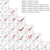 |
Fig. D.1 Correlation diagrams of the methods used to estimate cloud distances. |
Appendix D.107: G334.65+2.67
The CO radio observations by Dame et al. (2001) show two bright components of similar intensities with similar spatial distribution in the field. The first component has a velocity of ~−27 km s-1 typical of the Far Carina Arm (~15 kpc, Dame et al. 2001; Efremov 2011), whereas the second component has a velocity of ~3 km s-1 which indicates a much closer location (e.g. in Lupus with a distance ~150 pc, Tothill et al. 2009). Therefore, sources at both distances probably overlay in the field, making the determination of distance of individual sources out of reach of this paper. Therefore, we do not adopt any distance for this field.
Appendix D.108: G339.22-6.02
Our two distance estimates from extinction method, 8.63 ± 0.27 kpc (small aperture) and 2.09 ± 0.01 kpc (large aperture), are incompatible. The first one is of limited quality mainly because of a weakly significant cloud detection, and has a surprisingly large value. The second one has a very low agreement probability , but this can be due to the very large number of stars, and the cloud is clearly detected. Therefore we adopt the second estimate, but with a reliability flag of 0, and with a larger uncertainty of 1 kpc.
Appendix D.109: G341.18+6.51
This cloud is Lupus 6, a cloud part of the Lupus molecular complex (see Fig. 6 in Lombardi et al. 2008a). Lombardi et al. (2008b) report a distance of 155 ± 8 pc for the complex using
a combination of 2MASS extinction maps and Hipparcos and Tycho parallaxes. We adopt their value with a reliability flag of 2.
Appendix D.110: G343.64-2.31
The CO radio observations by Dame et al. (2001) show one bright component with velocity ~−15.5 km s-1. Otrupcek et al. (2000) made pointed CO (J = 1 → 0) observations towards the centre of this cloud. They found two components, a strong one at −15.3 km s-1 with TA = 8.9 K and a FWHM Δv = 7.1 km s-1, and a fainter one at −6.6 km s-1 with TA = 4.7 K and a FWHM Δv = 0.9 km s-1. This second component is completely missed in Dame et al. (2001) due to its low spectral resolution. They correspond respectively to kinematic distances between 1.33 kpc (V0 = 0 km s-1) and 1.78 (V0 = −15 km s-1) kpc, and between 0.46 kpc (V0 = 0 km s-1) and 0.96 kpc (V0 = −15 km s-1). Our extinction estimates give the results of 0.91 ± 0.78 kpc and 0.91 ± 0.70 kpc with good characteristics but large uncertainties. As a comparison, our previous estimate in Paper III was 1.10 kpc, derived using a previous version of the extinction method of Marshall et al. (2009) and for a slightly different area of the same cloud. Considering that the first CO component is much brighter, we favour its kinematic estimates, which are reasonably consistent with the extinction estimates when considering the uncertainties. We adopt a distance of 1.5 ± 0.5 kpc with a reliability flag of 1.
Appendix D.111: G344.77+7.58
The CO radio observations by Dame et al. (2001) show one component with velocity ~2 km s-1. This corresponds to too small distances for kinematic estimates to be reliable. The extinction estimates are ≲240 ± 230 pc (small aperture) and 200 ± 180 pc (large aperture), but with low reliability. For want of better data, we adopt a distance of 240 ± 240 pc with a reliability flag of 0.
Appendix D.112: G345.39-3.97
This cloud was studied by Racca et al. (2009) (their cloud BHR140) who determined a distance of 225 pc. We adopt their estimate with an uncertainty of 25 pc and reliability flag of 1.
Appendix D.113: G358.96+36.75
The distance to this cloud was estimated to 110 ± 10 pc by Franco (1989). We adopt this value, as in Paper III with a reliability flag of 1.
Appendix D.114: Comparison of methods
Figure D.1 compares the distance estimates from the various methods used in this paper.
Appendix E: Size-Mass relation as a function of distance
In Fig. 13 we presented the size-mass diagram of all sources in our catalogue with a reliable distance estimate (distance reliability flag of 1 and 2). Similar figures are provided here as a function of distance.
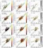 |
Fig. E.1 Mass–size diagrams for the galactic sources of our catalogue with distances between 0 and 200 pc (first row), 200 and 400 pc (second row), 400 and 600 pc (third row), and 600 and 800 pc (forth row). The masses are derived as explained in Sect. 4.2 and the sizes are the deconvolved linear sizes derived from getsources output for the column density map. As a comparison, the pale green band and white lines show the correlation observed for CO clumps (Elmegreen & Falgarone 1996). The two solid black lines indicate the loci for critical isothermal Bonnor-Ebert spheres at T = 7 K (lower line) and T = 20 K (upper line). The colour scale indicates the distance of sources in frame a), and the dust colour temperature of sources in frame b). Frame c) compares the location of starless sources (grey scale) to protostellar sources (points). The bin-averaged temperature curves for starless and protostellar sources are over-plotted in green and orange, respectively. The vertical bars are the standard deviations for each bin-average. |
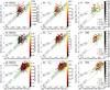 |
Fig. E.2 Same as Fig. E.1 with distances between 800 pc and 1 kpc (first row), 1 kpc and 1.5 kpc (second row), and greater than 1.5 kpc (third row). |
Appendix F: Cumulative fraction of background column density as a function of distance
In Fig. 17 (top left) we presented the cumulative fraction of background column density of all Galactic sources in our catalogue. Similar figures are provided here as a function of distance.
Appendix G: Maps of observed and derived quantities
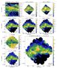 |
Fig. G.1 Data on the field G3.08+9.38. |
 |
Fig. G.2 Data on the field G21.26+12.11. |
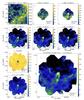 |
Fig. G.3 Data on the field G26.34+8.65. |
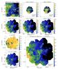 |
Fig. G.4 Data on the field G37.91+2.18. |
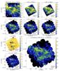 |
Fig. G.5 Data on the field G70.10-1.69. |
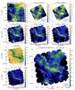 |
Fig. G.6 Data on the field G82.65-2.00. |
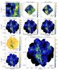 |
Fig. G.7 Data on the field G98.00+8.75. |
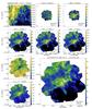 |
Fig. G.8 Data on the field G108.28+16.68. |
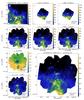 |
Fig. G.9 Data on the field G109.80+2.70 (also referred to as PCC288). |
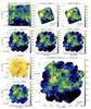 |
Fig. G.10 Data on the field G111.41-2.95. |
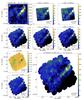 |
Fig. G.11 Data on the field G139.60-3.06. |
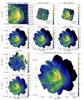 |
Fig. G.12 Data on the field G141.25+34.37. |
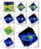 |
Fig. G.13 Data on the field G155.80-14.24. |
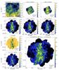 |
Fig. G.14 Data on the field G157.08-8.69 (also referred to as v31_7488). |
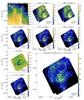 |
Fig. G.15 Data on the field G159.23-34.51. |
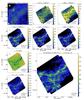 |
Fig. G.16 Data on the field G163.82-8.44 (also referred to as v31_7420). |
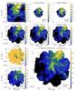 |
Fig. G.17 Data on the field G174.22+2.58. |
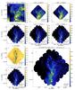 |
Fig. G.18 Data on the field G202.02+2.85. |
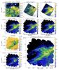 |
Fig. G.19 Data on the field G271.51+5.14. |
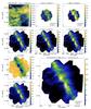 |
Fig. G.20 Data on the field G300.86-9.00 (also referred to as PCC550). |
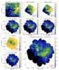 |
Fig. G.21 Data on the field G343.64-2.31. |
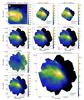 |
Fig. G.22 Data on the field G358.96+36.75 (also referred to as v31_0035). |
All Tables
All Figures
|
Fig. 1 Herschel fields of the Galactic Cold Cores programme shown in blue on the velocity-integrated CO map (Dame et al. 2001) of the Galaxy (colour scale, in K km s-1). Thirteen fields have absolute galactic latitude greater than 25 deg and do not appear on this map. |
| In the text | |
|
Fig. 2 Distance estimates for 108 of the 116 fields observed for the Galactic Cold Cores programme. The values and their associated uncertainties adopted in this paper are shown by the horizontal red lines and the grey areas, respectively. Fields with a reliable value-uncertainty pair (distance flag = 2) are in bold text. Grey text indicates fields with unreliable or no final estimates (distance flag = 0). No data could be found or produced for the five missing fields (G71.27-11.32, G128.78-69.46, G171.35-38.28, G218.06+2.12, and G299.57+5.61). For each field, all available estimates are shown. Stars with different colours indicate data found in the literature. The various methods are colour coded as presented in the upper panel and explained in Sect. 3.1. All numerical values are given in Table D.1, and individual sources are discussed in Appendix D. |
| In the text | |
|
Fig. 3 Example of association between a Herschel target and an object with known distance in the case of the field G202.02+2.85 apparently connected with the stellar open cluster NGC 2264. The colour scale shows the relative intensity in the WISE 12 μm band. White and red contours are 0 and 100 MJy intensity levels from the Herschel 250 μm band and emphasise the map edges and the submillimetre mapped filament, respectively. The purple stars are those associated with NGC 2264 according to the SIMBAD database. |
| In the text | |
|
Fig. 4 Left: Galactic latitudes (orange points) and altitudes (black points) of our fields compared to the histogram of field distances. Open circles are for fields with unreliable distance estimates. Broken lines show the average values over distance bins. The contribution of fields with unreliable distance estimates to the distance histogram is shown in light grey. Right: same as left but for galactic longitude (orange) and galactic radius (black). |
| In the text | |
|
Fig. 5 90% percentile of dust temperature T90% (left) and median column density (right) of fields as functions of position in the Galaxy. In the lower panels, the X and Y coordinates define positions in the Galactic plane with the Galactic centre at (X,Y) = (0,0), the Sun at (X,Y) = (8400 pc,0), and 0 ≤ l ≤ 180 deg for Y ≤ 0. The shaded arcs are the Carina-Sagittarius arm (I), the local arm (II), and the Perseus arm (III), as parametrised by Hou & Han (2014, their Table 1, three-arm model with all spiral tracers). |
| In the text | |
|
Fig. 6 Data on the field G176.27-2.09. Shown are the surface brightness maps for WISE 22 μm (frame a), 12′′ resolution), PACS 100 μm (frame b), 7.7′′ resolution), PACS 160 μm (frame c), 12′′ resolution), SPIRE 250 μm (frame d), 18.1′′ resolution), SPIRE 350 μm (frame e), 25.2′′ resolution), and SPIRE 500 μm (frame f), 38.5′′ resolution). The dust colour temperature map (frame g), 40′′ resolution) and H2 column density map (frame h), 40′′ resolution) are derived from SPIRE data. The beam sizes are indicated in the lower left corner of each frame. The FWHM ellipses of sources are shown in frame i) plotted on the SPIRE 250 μm map. Candidate galaxies, protostellar, and starless sources are indicated with white triangles, red stars, and blue filled circles, respectively. Ellipses without additional symbols are galactic sources at an undetermined stage of evolution. The red ellipses in frame e) show the positions of Planck sources from the PGCC catalogue (Planck Collaboration XXVIII 2015). In frames c)−f), and h), the white solid line shows the boundary of the mask employed for the source extraction. |
| In the text | |
|
Fig. 7 Pixel-by-pixel spectral energy distributions of a starless cold core (left; source ID = 1466, α = 100.32654, δ = 10.42901, in G202.02+2.85) and a cold core hosting a known young stellar object (right; source ID = 3863, α = 343.42069, δ = 62.533048, in G109.80+2.70 = PCC288). Each pixel is 20′′. Shown are the fluxes at 100 and 160 μm from PACS and 250, 350, and 500 μm from SPIRE. The fluxes at 3.4, 4.6, 12, and 22 μm from WISE are also shown, but are high enough to be visible only near the protostar in the right panel. The blue lines are the best fit of the four longest wavelengths using a modified black body with a fixed spectral index β = 2. The corresponding colour temperature is indicated in the top left corner of each pixel, in units of kelvin. The backgrounds are filled contour maps of the 250 μm surface brightness. The large and small red ellipses are the FWHM and footprint of the sources, respectively, as given by getsources for the column density map. The red cross shows the centre position of the source. In the bottom left corners, red points show the SED derived from getsources total fluxes of the sources for 160 μm from PACS and 250, 350, and 500 μm from SPIRE. |
| In the text | |
|
Fig. 8 WISE and Herschel sources on WISE 12 μm (left) and Herschel 250 μm (right) brightness maps. From the WISE PSC, only sources classified as Class I, Class II, shocked H2 gas, and resolved PAH emission according to the Koenig et al. (2012) criteria are shown. For Herschel sources the symbols are as in Fig. 6. Herschel sources classified as protostellar but presenting no association with a WISE protostar were classified from submillimetre data (see Sect. 4.4.1). |
| In the text | |
|
Fig. 9 Histograms of source distances, stacked over source type. |
| In the text | |
|
Fig. 10 Example of completeness analysis in the case of G202.02+2.85. Upper panel: surface brightness map of G202.02+2.85 in the 250 μm band for the true observations (left) and after adding isothermal Bonnor-Ebert sources (right). Lower panel: the black line histogram shows the mass spectrum of the added Bonnor-Ebert sources. The grey histogram represents the mass spectrum of the sources detected by getsources. The red points are the bin-by-bin ratio of the two histograms with statistical error bars defined by 1/ |
| In the text | |
|
Fig. 11 a) Distributions of the angular deconvolved sizes of all galactic sources with distance flags [1] or [2]. The black histogram is for all galactic sources (All), green for starless sources (SL), and orange for protostellar sources (PS, flags [1] and [2]). b) Distribution of the elongation of galactic sources. c) Distributions of the linear deconvolved sizes of galactic sources. The dashed histogram is for protostellar sources with a classification flag of [2]. d) Same as frame c) after selecting sources with angular sizes larger than 60′′ for both major and minor axes. The vertical dashed lines show the size of 0.2 pc. |
| In the text | |
|
Fig. 12 Mean column density − dust colour temperature diagrams for the galactic sources of our catalogue with distance flags 1 or 2. The colour scale indicates the mean particle density of sources in frame a), and the source submillimetre luminosity in frame b). Frame c) compares the location of protostellar sources (points) to starless sources (grey scale). The grey scale is the starless source density in the diagram, i.e. the number of sources per bin of temperature and column density. Orange triangles: protostellar sources with flag [1] from method A (tip-down) or B (tip-up). Red diamonds: protostellar sources from both methods (flag [2]). Blue circles: protostellar sources with AKARI 65 μm counterpart. The bin-averaged temperature curves for starless and protostellar sources are over-plotted in green and orange, respectively. The vertical bars are the standard deviations for each bin-average. The black contour contains ~75% of the sources shown in frame a), and is repeated in each frame to facilitate the comparison. |
| In the text | |
|
Fig. 13 Mass–size diagrams for the galactic sources of our catalogue with distance flags 1 or 2. The masses are derived as explained in Sect. 4.2 and the sizes are the deconvolved linear sizes derived from the getsources output for the column density map. As a comparison, the pale green band and white lines show the correlation observed for CO clumps (Elmegreen & Falgarone 1996). The two solid black lines indicate the loci for critical isothermal Bonnor-Ebert spheres at T = 7 K (lower line) and T = 20 K (upper line). The colour scale indicates the distance of sources in frame a), and the dust colour temperature of sources in frame b). Frame c) compares the location of protostellar sources (points) to starless sources (grey scale). Orange triangles: protostellar sources with flag [1] from method A (tip-down) or B (tip-up). Red diamonds: protostellar sources from both methods (flag [2]). Blue circles: protostellar sources with AKARI 65 μm counterpart. The bin-averaged mass curves for starless and protostellar sources are overplotted in green and orange, respectively. The vertical bars are the standard deviations for each bin average. |
| In the text | |
|
Fig. 14 Stability of sources as measured from the mass ratio αBE. Only sources classified as cores and with distance flags 1 or 2 are shown. a) Starless (green) vs. protostellar (orange hatched) cores for all distances (solid lines) and for distance estimates between 500 and 800 pc (dashed lines). The vertical red line indicates the αBE = 2 position. b)αBE is colour coded and represented against N(H2) and Tdust, as in Fig. 12. The black contour is repeated from Fig. 12. c)αBE is colour coded and represented against cores mass and deconvolved linear size. The blue contour shows the loci of cores with distance estimates between 500 and 800 pc. As a comparison, the pale green band and white lines show the correlation observed for CO clumps (Elmegreen & Falgarone 1996). The red lines in frames b) and c) show the αBE = 2 contours. |
| In the text | |
|
Fig. 15 Core mass function (CMF) per bin of distance. The corresponding upper and lower limits of distance bins are indicated below each CMF in units of kpc. Black dashed lines are for all sources (cores + clumps), black solid lines are for all cores, and green lines for starless cores. The error bars represent the statistical error. Red vertical dashed and dotted lines show the geometrical mean of completeness at 50% and 90%, respectively (see text for details). The y-axis is set for the lower distance bin. A vertical shift by 103 was added for each next upper distance bin. The bottom right insert shows the peak positions of every CMF, defined as the peak of the best log-normal fit, as a function of the central values of distance bins. The top left insert shows the slope dN/ d(log M) of the power-law fit of the high-mass tail as a function of the central values of distance bins. In both inserts, black circles are for CMF of all sources, green squares are for starless sources. The blue solid line shows the Mpeak ∝ D2 relation. |
| In the text | |
|
Fig. 16 Upper panel: dust temperature − mass diagram. The solid black contour contains 90% of all the sources. The grey scale shows the source surface density in the diagram for starless sources. Orange triangles: protostellar sources with flag [1] from method A (tip-down) or B (tip-up). Red diamonds: protostellar sources from both methods (flag [2]). Blue circles: protostellar sources with AKARI 65 μm counterpart. The green and orange step lines are the dust temperatures averaged over bins of the log 10 of source masses for starless and protostellar sources, respectively. The vertical bars are the reduced standard deviations for each bin-average and show that the two populations are significantly separated, on average. Lower left panel: peak position of the best log-normal fit of the reduced CMF as a function of the field-averaged source temperature. Black points are for all sources, green squares are for starless sources, and orange diamonds are for protostellar sources. Lower right panel: same as lower left panel but for the slope of the best power-law fit of the high-mass tail of the reduced CMF. |
| In the text | |
|
Fig. 17 Cumulative fraction of sources as a function of the background visual extinction. The top left frame compares starless (green) and protostellar (orange) sources. Solid lines are for all sources, dashed lines are for cores with αBE< 2. The top right frame shows, for all sources, the number of sources per bin of background column density and the mean fraction of starless (SL, green line) and protostellar (PS, orange line) sources in each bin. The bottom left frame shows the values of visual extinction AV at 50% of cumulative fraction for different bins of distance. Solid black lines are for all sources, red dashed lines for cores with αBE< 2. The bottom right frame shows the cumulative fractions for sources with αBE< 2 obtained per bin of field 9th decile temperatures T90%. The insert shows the variations in visual extinction AV at 50% of cumulative fraction as a function of T90%. The orange solid line shows Eq. (7) for β = 2, α = 4.5, and Tth = 12 K without fitting the data. The error bars in the insert and in the bottom left frame are proportional to 1/ |
| In the text | |
|
Fig. A.1 Distribution of the shift between the centre of the Herschel sources and the matching WISE sources. The black histogram and black circles show the shift distribution regardless of the classification method flag. The red histogram and red triangles show the shift distribution of sources with flag 2, i.e. classified as protostellar by methods A and B (Sect. 4.4.3). Upper panel: protostellar sources with embedded Class I and/or Class II YSOs. The scatter plot shows the correlation between the absolute and relative shifts with respect to the Herschel source size. The vertical dashed line shows the beam size. Lower panel: protostellar sources with AKARI 65 μm counterparts. Blue circles show sources classified as protostellar with embedded Class 0 YSOs. The scatter plot shows the absolute shift in WISE and AKARI source positions as a function of the absolute shift in WISE and Herschel source positions. |
| In the text | |
|
Fig. A.2 WISE colour−magnitude and colour−colour diagrams for classification of sources, showing the colour−magnitude and colour−colour criteria (black lines), AGN-classified sources (grey points with black edges), PAH/star forming galaxy-classified sources (white), shock-classified sources (yellow), resolved PAH emission-classified sources (purple), Class I-classified sources (red), Class II-classified sources (orange), and unclassified sources (small grey points without edges). |
| In the text | |
|
Fig. C.1 Left: close-up view of G163.82-8.44 centred at RA = 4h28m01.8s Dec = +36°45m51.87s. The colour scale shows the H2 column density derived from SPIRE data. The cyan ellipses show the FWHM of the sources obtained using getsources. Middle and right frames show the same field with simulated distances 3 and 10 times greater than the estimated distance of 0.42 kpc. |
| In the text | |
|
Fig. C.2 a) Source mass function of the G163.82-8.44 field for several values of the simulated distance. b) Number of sources (red circles) and average of the logarithm of source masses (orange squares) as functions of the simulated distance. The vertical bars show the standard deviation of the logarithm of source masses. The solid grey line shows a power law with exponent 2 on the right y-axis. Dotted and dashed lines are plotted to guide the eye. c) Histogram of dust colour temperature Tdust of G163.82-8.44 sources for several values of the simulated distance. In the inset, orange squares show the average values of Tdust and the vertical bars show the standard deviation of Tdust as functions of the simulated distance. |
| In the text | |
|
Fig. D.1 Correlation diagrams of the methods used to estimate cloud distances. |
| In the text | |
|
Fig. E.1 Mass–size diagrams for the galactic sources of our catalogue with distances between 0 and 200 pc (first row), 200 and 400 pc (second row), 400 and 600 pc (third row), and 600 and 800 pc (forth row). The masses are derived as explained in Sect. 4.2 and the sizes are the deconvolved linear sizes derived from getsources output for the column density map. As a comparison, the pale green band and white lines show the correlation observed for CO clumps (Elmegreen & Falgarone 1996). The two solid black lines indicate the loci for critical isothermal Bonnor-Ebert spheres at T = 7 K (lower line) and T = 20 K (upper line). The colour scale indicates the distance of sources in frame a), and the dust colour temperature of sources in frame b). Frame c) compares the location of starless sources (grey scale) to protostellar sources (points). The bin-averaged temperature curves for starless and protostellar sources are over-plotted in green and orange, respectively. The vertical bars are the standard deviations for each bin-average. |
| In the text | |
|
Fig. E.2 Same as Fig. E.1 with distances between 800 pc and 1 kpc (first row), 1 kpc and 1.5 kpc (second row), and greater than 1.5 kpc (third row). |
| In the text | |
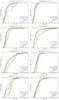 |
Fig. F.1 Same as Fig. 17, per bins of distances. |
| In the text | |
|
Fig. G.1 Data on the field G3.08+9.38. |
| In the text | |
|
Fig. G.2 Data on the field G21.26+12.11. |
| In the text | |
|
Fig. G.3 Data on the field G26.34+8.65. |
| In the text | |
|
Fig. G.4 Data on the field G37.91+2.18. |
| In the text | |
|
Fig. G.5 Data on the field G70.10-1.69. |
| In the text | |
|
Fig. G.6 Data on the field G82.65-2.00. |
| In the text | |
|
Fig. G.7 Data on the field G98.00+8.75. |
| In the text | |
|
Fig. G.8 Data on the field G108.28+16.68. |
| In the text | |
|
Fig. G.9 Data on the field G109.80+2.70 (also referred to as PCC288). |
| In the text | |
|
Fig. G.10 Data on the field G111.41-2.95. |
| In the text | |
|
Fig. G.11 Data on the field G139.60-3.06. |
| In the text | |
|
Fig. G.12 Data on the field G141.25+34.37. |
| In the text | |
|
Fig. G.13 Data on the field G155.80-14.24. |
| In the text | |
|
Fig. G.14 Data on the field G157.08-8.69 (also referred to as v31_7488). |
| In the text | |
|
Fig. G.15 Data on the field G159.23-34.51. |
| In the text | |
|
Fig. G.16 Data on the field G163.82-8.44 (also referred to as v31_7420). |
| In the text | |
|
Fig. G.17 Data on the field G174.22+2.58. |
| In the text | |
|
Fig. G.18 Data on the field G202.02+2.85. |
| In the text | |
|
Fig. G.19 Data on the field G271.51+5.14. |
| In the text | |
|
Fig. G.20 Data on the field G300.86-9.00 (also referred to as PCC550). |
| In the text | |
|
Fig. G.21 Data on the field G343.64-2.31. |
| In the text | |
|
Fig. G.22 Data on the field G358.96+36.75 (also referred to as v31_0035). |
| In the text | |
Current usage metrics show cumulative count of Article Views (full-text article views including HTML views, PDF and ePub downloads, according to the available data) and Abstracts Views on Vision4Press platform.
Data correspond to usage on the plateform after 2015. The current usage metrics is available 48-96 hours after online publication and is updated daily on week days.
Initial download of the metrics may take a while.