| Issue |
A&A
Volume 554, June 2013
|
|
|---|---|---|
| Article Number | A140 | |
| Number of page(s) | 19 | |
| Section | Cosmology (including clusters of galaxies) | |
| DOI | https://doi.org/10.1051/0004-6361/201220247 | |
| Published online | 18 June 2013 | |
Planck intermediate results
X. Physics of the hot gas in the Coma cluster
1 APC, AstroParticule et Cosmologie, Université Paris Diderot, CNRS/IN2P3, CEA/lrfu, Observatoire de Paris, Sorbonne Paris Cité, 10 rue Alice Domon et Léonie Duquet, 75205 Paris Cedex 13 France
2 Aalto University Metsähovi Radio Observatory, Metsähovintie 114, 02540 Kylmälä, Finland
3 Academy of Sciences of Tatarstan, Bauman Str. 20, 420111 Kazan, Republic of Tatarstan, Russia
4 Agenzia Spaziale Italiana Science Data Center, c/o ESRIN, via Galileo Galilei, Frascati, Italy
5 Agenzia Spaziale Italiana, Viale Liegi 26, Roma, Italy
6 Astrophysics Group, Cavendish Laboratory, University of Cambridge, J J Thomson Avenue, Cambridge CB3 0HE, UK
7 Atacama Large Millimeter/submillimeter Array, ALMA Santiago Central Offices, Alonso de Cordova 3107, Vitacura, Casilla 763 0355, Santiago, Chile
8 CITA, University of Toronto, 60 St. George St., Toronto, ON M5S 3H8, Canada
9 CNRS, IRAP, 9 Av. colonel Roche, BP 44346, 31028 Toulouse Cedex 4, France
10 California Institute of Technology, Pasadena, California, USA
11 Centre of Mathematics for Applications, University of Oslo, Blindern, Oslo, Norway
12 Centro de Astrofísica, Universidade do Porto, Rua das Estrelas, 4150-762 Porto, Portugal
13 Centro de Estudios de Física del Cosmos de Aragón (CEFCA), Plaza San Juan 1, planta 2, 44001 Teruel, Spain
14 Computational Cosmology Center, Lawrence Berkeley National Laboratory, Berkeley, California, USA
15 Consejo Superior de Investigaciones Científicas (CSIC), Madrid, Spain
16 DSM/Irfu/SPP, CEA-Saclay, 91191 Gif-sur-Yvette Cedex, France
17 DTU Space, National Space Institute, Technical University of Denmark, Elektrovej 327, 2800 Kgs. Lyngby, Denmark
18 Département de Physique Théorique, Université de Genève, 24 Quai E. Ansermet, 1211 Genève 4, Switzerland
19 Departamento de Física Fundamental, Facultad de Ciencias, Universidad de Salamanca, 37008 Salamanca, Spain
20 Departamento de Física, Universidad de Oviedo, Avda. Calvo Sotelo s/n, Oviedo, Spain
21 Department of Astronomy and Geodesy, Kazan Federal University, Kremlevskaya Str., 18, 420008 Kazan, Russia
22 Department of Astrophysics/IMAPP, Radboud University Nijmegen, PO Box 9010, 6500 GL Nijmegen, The Netherlands
23 Department of Physics & Astronomy, University of British Columbia, 6224 Agricultural Road, Vancouver, British Columbia, Canada
24 Department of Physics and Astronomy, Dana and David Dornsife College of Letter, Arts and Sciences, University of Southern California, Los Angeles, CA 90089, USA
25 Department of Physics and Astronomy, University of Iowa, 203 Van Allen Hall, Iowa City, IA 52242, USA
26 Department of Physics, Gustaf Hällströmin katu 2a, University of Helsinki, Helsinki, Finland
27 Department of Physics, Princeton University, Princeton, New Jersey, USA
28 Department of Physics, University of California, Berkeley, California, USA
29 Department of Physics, University of California, One Shields Avenue, Davis, California, USA
30 Department of Physics, University of California, Santa Barbara, California, USA
31 Department of Physics, University of Illinois at Urbana-Champaign, 1110 West Green Street, Urbana, Illinois, USA
32 Department of Statistics, Purdue University, 250 N. University Street, West Lafayette, Indiana, USA
33 Dipartimento di Fisica e Astronomia G. Galilei, Università degli Studi di Padova, via Marzolo 8, 35131 Padova, Italy
34 Dipartimento di Fisica, Università La Sapienza, P.le A. Moro 2, Roma, Italy
35 Dipartimento di Fisica, Università degli Studi di Milano, via Celoria 16, Milano, Italy
36 Dipartimento di Fisica, Università degli Studi di Trieste, via A. Valerio 2, Trieste, Italy
37 Dipartimento di Fisica, Università di Ferrara, via Saragat 1, 44122 Ferrara, Italy
38 Dipartimento di Fisica, Università di Roma Tor Vergata, via della Ricerca Scientifica 1, Roma, Italy
39 Dipartimento di Matematica, Università di Roma Tor Vergata, via della Ricerca Scientifica 1, Roma, Italy
40 Discovery Center, Niels Bohr Institute, Blegdamsvej 17, Copenhagen, Denmark
41 Dpto. Astrofísica, Universidad de La Laguna (ULL), 38206 La Laguna, Tenerife, Spain
42 European Southern Observatory, ESO Vitacura, Alonso de Cordova 3107, Vitacura, Casilla 19001, Santiago, Chile
43 European Space Agency, ESAC, Planck Science Office, Camino bajo del Castillo s/n, Urbanización Villafranca del Castillo, Villanueva de la Cañada, Madrid, Spain
44 European Space Agency, ESTEC, Keplerlaan 1, 2201 AZ Noordwijk, The Netherlands
45 GEPI, Observatoire de Paris, Section de Meudon, 5 place J. Janssen, 92195 Meudon Cedex, France
46 Helsinki Institute of Physics, Gustaf Hällströmin katu 2, University of Helsinki, Helsinki, Finland
47 INAF – Osservatorio Astrofisico di Catania, via S. Sofia 78, Catania, Italy
48 INAF – Osservatorio Astronomico di Padova, Vicolo dell’Osservatorio 5, 35131 Padova, Italy
49 INAF – Osservatorio Astronomico di Roma, via di Frascati 33, Monte Porzio Catone, Italy
50 INAF – Osservatorio Astronomico di Trieste, via G.B. Tiepolo 11, Trieste, Italy
51 INAF, Istituto di Radioastronomia, via P. Gobetti 101, 40129 Bologna, Italy
52 INAF/IASF Bologna, via Gobetti 101, Bologna, Italy
53 INAF/IASF Milano, via E. Bassini 15, Milano, Italy
54 INFN, Sezione di Roma 1, Università di Roma Sapienza, Piazzale Aldo Moro 2, 00185 Roma, Italy
55 INRIA, Laboratoire de Recherche en Informatique, Université Paris-Sud 11, Bâtiment 490, 91405 Orsay Cedex, France
56 Institut de Planétologie et d’Astrophysique de Grenoble (IPAG), Université Joseph Fourier Grenoble 1/CNRS-INSU, UMR 5274, 38041 Grenoble, France
57 ISDC Data Centre for Astrophysics, University of Geneva, ch. d’Ecogia 16, Versoix, Switzerland
58 IUCAA, Post Bag 4, Ganeshkhind, Pune University Campus, 411 007 Pune, India
59 Imperial College London, Astrophysics group, Blackett Laboratory, PrinceConsort Road, London, SW7 2AZ, UK
60 Infrared Processing and Analysis Center, California Institute of Technology, Pasadena, CA 91125, USA
61 Institut Néel, CNRS, Université Joseph Fourier Grenoble I, 25 rue des Martyrs, 38041 Grenoble, France
62 Institut Universitaire de France, 103 bd Saint-Michel, 75005 Paris, France
63 Institut d’Astrophysique Spatiale, CNRS UMR 8617, Université Paris-Sud 11, Bâtiment 121, Orsay, France
64 Institut d’Astrophysique de Paris, CNRS UMR 7095, 98bis boulevard Arago, 75014 Paris, France
65 Institute for Space Sciences, Bucharest-Magurale, Romania
66 Institute of Astro and Particle Physics, Technikerstrasse 25/8, University of Innsbruck, 6020 Innsbruck, Austria
67 Institute of Astronomy and Astrophysics, Academia Sinica, Taipei, Taiwan
68 Institute of Astronomy, University of Cambridge, Madingley Road, Cambridge CB3 0HA, UK
69 Institute of Theoretical Astrophysics, University of Oslo, Blindern, Oslo, Norway
70 Instituto de Astrofísica de Canarias, C/Vía Láctea s/n, La Laguna, Tenerife, Spain
71 Instituto de Física de Cantabria (CSIC-Universidad de Cantabria), Avda. de los Castros s/n, Santander, Spain
72 Jet Propulsion Laboratory, California Institute of Technology, 4800 Oak Grove Drive, Pasadena, California, USA
73 Jodrell Bank Centre for Astrophysics, Alan Turing Building, School of Physics and Astronomy, The University of Manchester, Oxford Road, Manchester, M13 9PL, UK
74 Kapteyn Astronomical Institute, University of Groningen, Landleven 12, 9747 AD Groningen, The Netherlands
75 Kavli Institute for Cosmology Cambridge, Madingley Road, Cambridge, CB3 0HA, UK
76 LAL, Université Paris-Sud, CNRS/IN2P3, Orsay, France
77 LERMA, CNRS, Observatoire de Paris, 61 avenue de l’Observatoire, Paris, France
78 Laboratoire AIM, IRFU/Service d’Astrophysique – CEA/DSM – CNRS – Université Paris Diderot, Bât. 709, CEA-Saclay, 91191 Gif-sur-Yvette Cedex, France
79 Laboratoire Traitement et Communication de l’Information, CNRS UMR 5141 and Télécom ParisTech, 46 rue Barrault, 75634 Paris Cedex 13, France
80 Laboratoire de Physique Subatomique et de Cosmologie, Université Joseph Fourier Grenoble I, CNRS/IN2P3, Institut National Polytechnique de Grenoble, 53 rue des Martyrs, 38026 Grenoble Cedex, France
81 Laboratoire de Physique Théorique, Université Paris-Sud 11 & CNRS, Bâtiment 210, 91405 Orsay, France
82 Lawrence Berkeley National Laboratory, Berkeley, California, USA
83 Max-Planck-Institut für Astrophysik, Karl-Schwarzschild-Str. 1, 85741 Garching, Germany
84 Max-Planck-Institut für Extraterrestrische Physik, Giessenbachstraße, 85748 Garching, Germany
85 MilliLab, VTT Technical Research Centre of Finland, Tietotie 3, Espoo, Finland
86 Minnesota Institute for Astrophysics, School of Physics and Astronomy, University of Minnesota, 116 Church St. SE, Minneapolis, MN 55455, USA
87 National University of Ireland, Department of Experimental Physics, Maynooth, Co. Kildare, Ireland
88 Niels Bohr Institute, Blegdamsvej 17, Copenhagen, Denmark
89 Observational Cosmology, Mail Stop 367-17, California Institute of Technology, Pasadena, CA, 91125, USA
90 Optical Science Laboratory, University College London, Gower Street, London, UK
91 SISSA, Astrophysics Sector, via Bonomea 265, 34136, Trieste, Italy
92 School of Physics and Astronomy, Cardiff University, Queens Buildings, The Parade, Cardiff, CF24 3AA, UK
93 Space Research Institute (IKI), Profsoyuznaya 84/32, Moscow, Russia
94 Space Research Institute (IKI), Russian Academy of Sciences, Profsoyuznaya Str. 84/32, 117997 Moscow, Russia
95 Space Sciences Laboratory, University of California, Berkeley, California, USA
96 Stanford University, Dept of Physics, Varian Physics Bldg, 382 via Pueblo Mall, Stanford, California, USA
97 TÜBİTAK National Observatory, Akdeniz University Campus, 07058 Antalya, Turkey
98 UPMC Univ. Paris 6, UMR7095, 98bis boulevard Arago, 75014 Paris, France
99 Universität Heidelberg, Institut für Theoretische Astrophysik, Albert-Überle-Str. 2, 69120 Heidelberg, Germany
100 Université Denis Diderot Paris 7, 75205 Paris Cedex 13, France
101 Université de Toulouse, UPS-OMP, IRAP, 31028 Toulouse Cedex 4, France
102 University Observatory, Ludwig Maximilian University of Munich, Scheinerstrasse 1, 81679 Munich, Germany
103 University of Granada, Departamento de Física Teórica y delCosmos, Facultad de Ciencias, Granada, Spain
104 University of Miami, Knight Physics Building, 1320 Campo Sano Dr., Coral Gables, Florida, USA
105 Warsaw University Observatory, Aleje Ujazdowskie 4, 00-478 Warszawa, Poland
Received: 17 August 2012
Accepted: 26 November 2012
Abstract
We present an analysis of Planck satellite data on the Coma cluster observed via the Sunyaev-Zeldovich effect. Thanks to its great sensitivity, Planck is able, for the first time, to detect SZ emission up to r ≈ 3 × R500. We test previously proposed spherically symmetric models for the pressure distribution in clusters against the azimuthally averaged data. In particular, we find that the Arnaud et al. (2010, A&A, 517, A92) “universal” pressure profile does not fit Coma, and that their pressure profile for merging systems provides a reasonable fit to the data only at r < R500; by r = 2 × R500 it underestimates the observed y profile by a factor of ≃2. This may indicate that at these larger radii either: i) the cluster SZ emission is contaminated by unresolved SZ sources along the line of sight; or ii) the pressure profile of Coma is higher at r > R500 than the mean pressure profile predicted by the simulations used to constrain the models. The Planck image shows significant local steepening of the y profile in two regions about half a degree to the west and to the south-east of the cluster centre. These features are consistent with the presence of shock fronts at these radii, and indeed the western feature was previously noticed in the ROSAT PSPC mosaic as well as in the radio. Using Plancky profiles extracted from corresponding sectors we find pressure jumps of 4.9-0.2+0.4 and 5.0-0.1+1.3 in the west and south-east, respectively. Assuming Rankine-Hugoniot pressure jump conditions, we deduce that the shock waves should propagate with Mach number Mw = 2.03-0.04+0.09 and Mse = 2.05-0.02+0.25 in the west and south-east, respectively. Finally, we find that the y and radio-synchrotron signals are quasi-linearly correlated on Mpc scales, with small intrinsic scatter. This implies either that the energy density of cosmic-ray electrons is relatively constant throughout the cluster, or that the magnetic fields fall off much more slowly with radius than previously thought.
Key words: galaxies: clusters: individual: Coma cluster / galaxies: clusters: intracluster medium / X-rays: galaxies: clusters / cosmology: observations / galaxies: clusters: general / cosmic background radiation
Corresponding author: P. Mazzotta, This email address is being protected from spambots. You need JavaScript enabled to view it.
© ESO, 2013
1. Introduction
The Coma cluster is the most spectacular Sunyaev-Zeldovich (SZ) source in the Planck sky. It is a low-redshift, massive, and hot cluster, and is sufficiently extended that Planck can resolve it well spatially. Its intracluster medium (ICM) was observed in SZ for the first time with the 5.5 m OVRO telescope (Herbig et al. 1992, 1995). Later, it was also observed with MSAM1 (Silverberg et al. 1997), MITO (De Petris et al. 2002), VSA (Lancaster et al. 2005) and WMAP (Komatsu et al. 2011) which detected the cluster with signal-to-noise ratio of S/N = 3.6. As reported in the all-sky early Sunyaev-Zeldovich cluster paper, Planck detected the Coma cluster with a S/N > 22 (Planck Collaboration 2011d).
Coma has also been extensively observed in the X-rays from the ROSAT all-sky survey and pointed observations (Briel et al. 1992; White et al. 1993), as well as via a huge mosaic by XMM-Newton (e.g. Neumann et al. 2001, 2003; Schuecker et al. 2004). The X-ray emission reveals many spatial features indicating infalling sub-clusters such as NGC 4839 (Dow & White 1995; Vikhlinin et al. 1997; Neumann et al. 2001, 2003) , turbulence (e.g. Schuecker et al. 2004; Churazov et al. 2012) and further signs of accretion and strong dynamical activity.
Moreover, the Coma cluster hosts a remarkable giant radio halo extending over 1 Mpc, which traces the non-thermal emission from relativistic electrons and magnetic fields (e.g. Giovannini et al. 1993; Brown & Rudnick 2011). The radio halo’s spectrum and extent require an ongoing, distributed mechanism for acceleration of the relativistic electrons, since their radiative lifetimes against synchrotron and inverse Compton losses are short, even compared to their diffusion time across the cluster (e.g. Sarazin 1999; Brunetti et al. 2001). The radio halo also appears to exhibit a shock front in the west, also seen in the X-ray image, and is connected at larger scales with a huge radio relic in the south-west (Ensslin et al. 1998; Brown & Rudnick 2011).
In this paper we present a detailed radial and sector analysis of the Coma cluster as observed by Planck. These results are compared with X-ray and radio observations obtained with XMM-Newton and the Westerbork Synthesis Radio Telescope.
We use H0 = 70 km s-1Mpc-1, Ωm = 0.3 and ΩΛ = 0.7, which imply a linear scale of 27.7 kpc arcmin-1 at the distance of the Coma cluster (z = 0.023). All the maps are in Equatorial J2000 coordinates.
2. The Planck frequency maps
Planck1 (Tauber et al. 2010; Planck Collaboration 2011a) is the third-generation space mission to measure the anisotropy of the cosmic microwave background (CMB). It observes the sky in nine frequency bands covering 30–857 GHz with high sensitivity and angular resolution from 31′ to 5′. The Low Frequency Instrument (LFI; Mandolesi et al. 2010; Bersanelli et al. 2010; Mennella et al. 2011) covers the 30, 44, and 70 GHz bands with amplifiers cooled to 20 K. The High Frequency Instrument (HFI; Lamarre et al. 2010; Planck HFI Core Team 2011a) covers the 100, 143, 217, 353, 545, and 857 GHz bands with bolometers cooled to 0.1 K. Polarisation is measured in all but the highest two bands (Leahy et al. 2010; Rosset et al. 2010). A combination of radiative cooling and three mechanical coolers produces the temperatures needed for the detectors and optics (Planck Collaboration 2011b). Two data processing centres (DPCs) check and calibrate the data and make maps of the sky (Planck HFI Core Team 2011b; Zacchei et al. 2011). Planck’s sensitivity, angular resolution, and frequency coverage make it a powerful instrument for Galactic and extragalactic astrophysics as well as for cosmology. Early astrophysics results are given in Planck Collaboration VIII-XXVI 2011, based on data taken between 13 August 2009 and 7 June 2010.
This paper is based on the Planck nominal survey of 14 months, i.e. taken between 13 August 2009 and 27 November 2010. The whole sky has been covered two times. We refer to Planck HFI Core Team (2011b) and Zacchei et al. (2011) for the generic scheme of time ordered information (TOI) processing and map making, as well as for the technical characteristics of the maps used. We adopt a circular Gaussian beam pattern for each frequency as described in these papers. We use the full-sky maps in the nine Planck frequency bands provided in HEALPix (Górski et al. 2005) Nside = 2048 resolution. An error map is associated with each frequency band and is obtained from the difference of the first half and second half of the Planck rings for a given position of the satellite, but are basically free from astrophysical emission. However, they are a good representation of the statistical instrumental noise and systematic errors. Uncertainties in flux measurements due to beam corrections, map calibrations and uncertainties in bandpasses are expected to be small, as discussed extensively in Planck Collaboration (2011d,c,e).
3. Reconstruction and analysis of the y map
The Comptonisation parameter y maps used in this work have been obtained using the MILCA (modified internal linear combination algorithm) method (Hurier et al. 2010) on the Planck frequency maps from 100 GHz to 857 GHz in a region centred on the Coma cluster. MILCA is a component separation approach aimed at extracting a chosen component (in our case the thermal Sunyaev Zeldovich, tSZ, signal) from a multi-channel set of input maps. It is based mainly on the well known ILC approach (see for example Eriksen et al. 2004), which searches for the linear combination of input maps that minimises the variance of the final reconstructed map while imposing spectral constraints. For this work, we apply MILCA using two constraints, the first to preserve the y signal and the second to remove CMB contamination in the final y map. Furthermore, we correct for the bias induced by the instrumental noise, and we simultaneously use the extra degrees of freedom (d.o.f.) to minimise residuals from other components (2 d.o.f.) and from the instrumental noise (2 d.o.f.). These would otherwise increase the variance of the final reconstructed y map. The noise covariance matrix is estimated from jack-knife maps. To improve the efficiency of the algorithm we perform our separation independently on several bins in the spatial-frequency plane. The final y map has an effective point spread function (PSF) with a resolution of 10′ FWHM. Finally, to characterise the noise properties, such as correlation and inhomogeneities, we use jack-knife and redundancy maps for each frequency and apply the same linear transformation as used to compute the MILCA y map. The MILCA procedure provides us with a data map y together with random realisations of an additive noise model dy, which is Gaussian, correlated, and may present some non-stationary behaviour across the field of view. These maps are used to derive radial profiles and to perform the image analysis, as described below.
We verified that the reconstruction methods GMCA (Bobin et al. 2008) and NILC (Remazeilles et al. 2011) give results that are consistent within the errors with the MILCA method (see Planck Collaboration 2013).
3.1. Analysis of radial profiles
In this paper, we present various radial profiles y(r) of the 2D distribution of the Comptonisation parameter y. These allow us to study the underlying pressure distribution of the ICM of Coma. The y parameter is proportional to the gas pressure P = nekT integrated along the line of sight:  (1)where ne and T are the gas electron density and temperature, σT is the Thomson cross-section, k the Boltzmann constant, me the mass of the electron and c the speed of light. All the radial profiles y(r) are extracted from the y map after masking out bright radio sources. In this work we model the observed y(r) projected profiles using the forward approach described in detail by e.g. Bourdin & Mazzotta (2008). We assume that the three-dimensional pressure profiles can be adequately represented by some analytic functions that have the freedom to describe a wide range of possible profiles. The 3D model is projected along the line of sight, assuming spherical symmetry and convolved with the Planck PSF to produce a projected model function f(r). Finally we fit f(r) to the data using a χ2 minimisation of its distance from the radial profiles y(r) + dy(r) derived from the MILCA map (y(r)) and 1000 realization of its additive noise model (dy(r)). The χ2 is calculated in the principal component basis of these noise realisations. This procedure uses an orthogonal transformation to diagonalise the noise covariance matrix which, thus, decorrelates the additive noise fluctuation.
It is important to say that, as the parameters of the fitting functions are highly degenerate, we adopt two techniques to quantify the uncertainties, i) for each individual parameter; and ii) for the overall model (that is, the global model envelope).
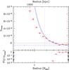 |
Fig. 1 Upper panel: radial profile of y in a set of circular annuli centred on Coma. The blue curve is the best fitting simple model to the profile over the radial range from 85 arcmin to 300 arcmin. The model consists of a power law plus a constant yoff. The best fitting value of yoff is shown with the dashed horizontal line. Two vertical lines indicate the range of radii used for fitting. Lower panel: the probability of finding an observed value of y > yComa in a given annulus. The probability was estimated by measuring y in a set of annuli with random centres in any part of the image outside 5 × R500, where R500 = 47 arcmin. |
More specifically, the confidence intervals on each parameter are calculated using the percentile method; i.e., we rank the fitted values and select the value corresponding to the chosen percentile. Suppose that our 1000 realizations for a specific parameter ζ are already ranked from bottom to top, the percentile confidence interval at 68.4% corresponds to [ζ158th,ζ842th]. Notice that in this work the confidence intervals are reported with respect to the best-fit value obtained by fitting the model to the initial data set.
The envelope of the profiles shown in Figs. 5–7, 11–14 delimit, instead, the first 684 out of the 1000 model profiles with the lowest χ2. Note that, by design, the forward approach tests the capability of a specific functional to globally reproduce the observed data. For this reason, the error estimates represent the uncertainties on the parameters of the fitting function rather than the local uncertainties of the deprojected quantity. This technique has been fully tested on hydrodynamic simulations (e.g. Nagai et al. 2007; Meneghetti et al. 2010).
3.2. Zero level of the y map and the maximum detection radius
As a result of the extraction algorithm, Plancky maps contain an arbitrary additive constant yoff which is a free parameter in all our y-map models. This constant can be determined using the Planck patch by simply setting to zero the y value measured at very large radii, where we expect to have small or no contribution to the signal from the Cluster itself. In particular, in the case of the 13.6deg × 13.6deg MILCA-based patch of the image centred on Coma, this constant is negative, as illustrated in Fig. 1. The radial profile of y was extracted from the y map in a set of circular annuli centred at (RA, Dec) = (12h59m47s, + 27°55′53″). The errors assigned to the points are crudely estimated by calculating the variance of the y map blocked to a pixel size much larger than the size of the Planck PSF. The variance is then rescaled for each annulus, assuming that the correlation of the noise can be neglected on these spatial scales. For a model consisting of a power law plus a constant (over the radial range from 85 arcmin to 300 arcmin) we find yoff = −6.3 × 10⁻⁷ ± 0.9 × 10⁻⁷. We note that the precise value of yoff depends weakly on the particular model used, and on the range of radii involved in the fitting.
To determine the maximum radius at which Planck detects a significant excess of y compared to the rest of the image, we adopted the following procedure. For every annulus around Coma with measured y = yComa we have calculated the distribution of y = yrandom measured in 300 annuli of a similar size, but with the centres randomly placed in any part of the image outside the 5 × R500 circle around Coma, where R500 is the radius at which the cluster density contrast is Δ = 500. When calculating yrandom the parts of the annuli within 5 × R500 were excluded. The comparison of yComa with the distribution of yrandom is used to conservatively estimate the probability of getting y > yComa by chance in an annulus of a given size at a random position in the image (see Fig. 1, lower panel). For the annulus between 2.6 and 3.1 R500 (122 arcmin to 147 arcmin) the probability of getting yComa by chance is ≈3 × 10⁻³ (a crude estimate, given N = 300 random positions). For smaller radii the probability is much lower, while at larger radii the probability of getting y in excess of yComa is ~10% or higher. We conclude that Planck detects the signal from Coma in narrow annuli ΔR/R = 0.2 at least up to Rmax ~ 3 × R500. This is a conservative and model-independent estimate. In the rest of the paper we use parametric models which cover the entire range of radii to fully exploit Planck data even beyond Rmax.
4. XMM-Newton data analysis
The XMM-Newton results presented in this paper have been derived from analysis of the mosaic obtained by combining 27 XMM-Newton pointings of the Coma cluster available in the archive. The XMM-Newton data have been prepared and analysed using the procedure described in detail in Bourdin et al. (2011), and Bourdin & Mazzotta (2008). We estimated the YX = Mgas × T parameter of Coma iteratively using the YX − M500 scaling relation calibrated from hydrostatic mass estimates in a nearby cluster sample observed with XMM-Newton (Arnaud et al. 2010); we find R500 ≈ (47 ± 1)arcmin ≈ (1.31 ± 0.03) Mpc and we use this value throughout the paper. To study the surface brightness and temperature radial profiles we use the forward approach described in Bourdin et al. (2011) taking care to project the temperature profile using the formula appropriate for spectroscopy; i.e., we use the spectroscopic-like temperature introduced by Mazzotta et al. (2004).
5. The Coma y maps
The main goal of this paper is to present the radial and sectoral properties of the SZ signal from the Coma cluster. Here we describe some general properties of the image; the full image analysis will be presented in a forthcoming paper that will make use of all the Planck data, including the extended surveys.
Figure 2 shows the Plancky map of the Coma cluster obtained by combining the HFI channels from 100 GHz to 857 GHz. The effective PSF of this map corresponds to FWHM = 10′ and its noise level is σnoise = 2.3 × 10⁻⁶.
To highlight the spatial structure of the y map, in Fig. 2 we overlay the contour levels of the y signal. We notice that at this resolution, the y signal observed by Planck traces the pressure distribution of the ICM up to R500. As is already known from X-ray observations (e.g. Briel et al. 1992; White et al. 1993; Neumann et al. 2003), the Plancky map shows that the gas in Coma is elongated towards the west and extends in the south-west direction toward the NGC 4839 subgroup. Fig. 2 shows that the SZ signal from this subgroup is clearly detected by Planck (see the white cross to the south-west).
Figure 2 also shows clear compression of the isocontour lines in a number of cluster regions. We notice that, in most cases, the extent of the compression is of the order of the y map correlation length (≈10′): it is likely that most of these are image artifacts induced by correlated noise in the y map. Nevertheless, we also notice at least two regions where the compression of the isocontour lines extends over angular scales significantly larger than the noise correlation length. These two regions, located to the west and to the southeast of cluster centre, may indicate real steepenings of the radial gradient. Such steepenings suggest the presence of a discontinuities in the cluster pressure profile, which may be produced by a thermal shocks, as we discuss in Sect. 7. For convenience, in Fig. 2 we outline the regions from which we extract the y profiles used in Sect. 7 with white sectors. It is worth noting that the western steepening extends over a much larger angular scale than indicated by the white sector. In Sect. 7 we explain why we prefer a narrower sector for our quantitative analysis.
In Fig. 3 we show the Plancky map of the Coma cluster obtained by adding the 70 GHz channel of LFI to the HFI channels and smoothing to a lower resolution. The PSF of this map corresponds to FWHM = 30′, which lowers the noise level by approximately one order of magnitude with respect to the 10′ resolution map: σnoise30 = 3.35 × 10⁻⁷. As for Fig. 2 the outermost contour level indicates y = 2 × σnoise30 = 6.7 × 10⁻⁷. Due to the larger smoothing, this map shows less structure in the cluster centre, but clearly highlights that Planck can trace the pressure profile of the ICM well beyond R200 ≈ 2 × R500 (see the outermost circle in Fig. 3).
6. Azimuthally averaged profile
Before studying the azimuthally averaged SZ profile of the Coma cluster in detail, we first show a very simple performance test. In Fig. 4 we compare the SZ effect toward the Coma cluster, in units of the Rayleigh-Jeans equivalent temperature, measured by Planck and by WMAP using the optimal V and W bands (from Fig. 14 of Komatsu et al. 2011). This figure shows that, in addition to its greatly improved angular resolution, Planck frequency coverage results in errors on the profile which are ≈20 times smaller than those from WMAP. Thanks to this higher sensitivity Planck allows us to study, for the first time, the SZ signal of the Coma cluster to its very outermost regions. We do this by extracting the radial profile in concentric annuli centred on the cluster centroid (RA, Dec)= (12h59m47s, + 27°55′53″).
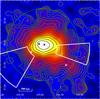 |
Fig. 2 The Plancky map of the Coma cluster obtained by combining the HFI channels from 100 GHz to 857 GHz. North is up and west is to the right. The map is corrected for the additive constant yoff. The final map bin corresponds to FWHM = 10′. The image is about 130 arcmin × 130 arcmin. The contour levels are logarithmically spaced by 21/4 (every 4 lines, y increases by a factor 2). The outermost contour corresponds to y = 2 × σnoise = 4.6 × 10⁻⁶. The green circle indicates R500. White and black crosses indicate the position of the brightest galaxies in Coma. The white sectors indicate two regions where the y map shows a local steepening of the radial gradient (see Sect. 7 and Fig. 6). |
We fit the observed y profile using the pressure formula proposed by Arnaud et al. (2010): ![Mathematical equation: \begin{equation} P(x)=\frac{P_0}{(c_{500}x)^\gamma\left[1+(c_{500}x)^{\alpha}\right]^{(\beta-\gamma)/\alpha}}, \label{eq:arnaud} \end{equation}](/articles/aa/full_html/2013/06/aa20247-12/aa20247-12-eq76.png) (2)where, x = (R/R500). This is done by fixing R500 at the best-fit value obtained from the X-ray analysis (R500 = 1.31 Mpc, see Sect. 4) and using three different combinations of parameters which we itemise below:
(2)where, x = (R/R500). This is done by fixing R500 at the best-fit value obtained from the X-ray analysis (R500 = 1.31 Mpc, see Sect. 4) and using three different combinations of parameters which we itemise below:
-
a “universal” pressure model (which we will refer to as Model A)for which we leave only P0 as a free parameter and fix c500 = 1.177, γ = 0.3081, α = 1.0510, β = 5.4905 (Arnaud et al. 2010);
-
a pressure profile appropriate for clusters with disturbed X-ray morphology (Model B) for which we leave P0 as a free parameter and fix c500 = 1.083, γ = 0.3798, α = 1.406, β = 5.4905 (Arnaud et al. 2010);
-
a modified pressure profile (Model C) for which we let all the parameters vary (except R500).
The best-fit parameters, together with their 68.4% confidence level errors, are reported in Table 1. The resulting best-fit models, together with the envelopes corresponding to the 68.4% of models with the lowest χ2, are overlaid in the upper left, upper right and lower left panels of Fig. 5, for models A, B, and C, respectively. We find that Eq. (2) fits the observed y profile only if all the parameters (except R500) are left free to vary (i.e., Model C).
We also fit the observed radial y profile using a fitting formula (Model D) derived from the density and temperature functionals introduced by Vikhlinin et al. (2006):  (3)where
 ![Mathematical equation: \begin{eqnarray} n_{\rm e}^2(r) &=& n_{0}^2 \frac{(r/r_{\rm c})^{-\alpha}}{[1+(r/r_{\rm c})^2]^{3\beta - \alpha/2}} \frac{1}{[1+(r/r_{\rm s})^3]^{\epsilon/3}} \nonumber \\ &&+ \frac {n_{02}^2}{[1+(r/r_{{\rm c}2})^2]^{3\beta_2}}, \label{rho3d_equ} \end{eqnarray}](/articles/aa/full_html/2013/06/aa20247-12/aa20247-12-eq88.png) (4)and
(4)and ![Mathematical equation: \begin{equation} T(r) = T_0 \frac{(r/r_{\rm t})^{-a}}{[1+(r/r_{\rm t})^b]^{c/b}}\cdot \label{t3d_equ} \end{equation}](/articles/aa/full_html/2013/06/aa20247-12/aa20247-12-eq89.png) (5)Notice that, for our purpose, Eq. (3) is only used to fit the cluster pressure profile. For this reason, it is unlikely that, when considered separately, the best-fit parameters of Eqs. (4) and (5) reproduce the actual cluster density and temperature profiles. The best-fit parameters, together with their 68.4% confidence level errors, are reported in Table 2.
(5)Notice that, for our purpose, Eq. (3) is only used to fit the cluster pressure profile. For this reason, it is unlikely that, when considered separately, the best-fit parameters of Eqs. (4) and (5) reproduce the actual cluster density and temperature profiles. The best-fit parameters, together with their 68.4% confidence level errors, are reported in Table 2.
The resulting model, with the 68.4% envelope is overlaid in the lower-right panel of Fig. 5. The above temperature and density functions contain many more free parameters than Eq. (2). All these parameters have been specifically introduced to adequately fit all the observed surface brightness and temperature profiles of X-ray clusters of galaxies. This function, thus, is capable, in principle, of providing a better fit to any observed SZ profile. Despite this, we find that compared with Model C, Model D does not improve the quality of the fit. The reduced χ2 of model D is slightly higher (Δχ2 = 0.3) than for model C.
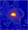 |
Fig. 3 The Plancky map of the Coma cluster obtained by combining the 70 GHz channel of LFI and the HFI channels from 100 GHz to 857 GHz. The map has been smoothed to have a PSF with FWHM = 30′. The image is about 266 arcmin × 266 arcmin. The outermost contour corresponds to y = 2 × σnoise30 = 6.7 × 10⁻⁷. The green circles indicate R500 and 2 × R500 ≈ R200. |
7. Pressure jumps
Figure 2 shows at least two cluster regions where the y isocontour lines appear to be compressed on angular scales larger than the correlation length of the noise map. This indicate a local steepening of the y signal. The most prominent feature is located at about 0.5 degrees from the cluster centre to the west. Its position angle is quite large and extends from 340 deg to 45 deg. The second, less prominent feature, is located at 0.5 degrees from the cluster center to the south-east.
Both features suggest the presence of discontinuities in the underlying cluster pressure profiles. To test this hypothesis and to try to estimate the amplitude and the position of the pressure jumps we use the following simplified approach: i) we select two sectors; ii) we extract the y profiles using circular annuli; and iii) assuming spherical symmetry, we fit them to a 3D pressure model with a pressure jump. This test requires that the extraction sectors are carefully selected. Ideally one would like to follow, as close as possible, the curvature of the y signal around the possible pressure jumps. It is clear, however, that this procedure cannot be done exactly but it may be somewhat arbitrary. The pressure jumps are unlikely to be perfectly spherically symmetric, thus, the sector selection depends also on what is initially thought to be the leading edge of the underlying pressure jump. Despite of this arbitrariness, our approach remain valid for the purpose of testing for the presence of a shock. As matter of fact, even if we choose a sector that does not properly sample the pressure jump, our action goes in the direction of mixing the signal from the pre- and post-pressure jump regions. This will simply result is a smoother profile which, when fitted with the 3D pressure model, will returns a smaller amplitude for the pressure jump itself. Thus, in the worst scenario, the measured pressure jumps would, in any case, represent a lower estimate of the jumps at the leading edges.
In order to minimise the mixing of pre- and post-shock signals, one can reduce the width of the analysis sector to the limit allowed by signal statistics. Indeed, for very high signal-to-noise, one could, in principle, extract the y signal along a line perpendicular to the leading edge of the shock. This would limit mixing of pre- and post shock signals to line-of-sight and beam effects. In the specific case of the Coma cluster we notice that the west feature is located in a higher signal-to-noise region than the south-east one. For this reason we decide to extract the west profile using a sector with an angular aperture smaller than the actual angular extent of this feature in the y map.
Following the above considerations, we set the centres and orientations of the west and the south-east sectors to the values reported in the first three columns of Table 3 and indicated in Fig. 2. In Sect. 9.3 below we demonstrate that, within the selected sectors, the SZ and the X-ray analyses give consistent results. This indicates that, despite the apparent arbitrariness in sector selection: i) these SZ-selected sectors are representative of the features under study and; ii) that the hypothesis of spherical symmetry is a good approximation, at least within the selected sectors.
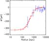 |
Fig. 4 Comparison of the radial profile of the SZ effect towards the Coma cluster, in units of the Rayleigh-Jeans equivalent temperature measured by Planck (crosses) with the one obtained by WMAP (open squares) using the optimal V and W band data (from Fig. 14 of Komatsu et al. 2011). The plotted Planck errors are the square root of the diagonal elements of the covariance matrix. Notice that profiles have been extracted from SZ maps with 10′ and 30′ angular resolution from Planck and WMAP, respectively. |
Best-fit parameters for the Arnaud et al. (2010) pressure model Eqs. (4) and (5).
We fit the profiles using a 3D pressure model composed of two power laws with index η1 and η2 and a jump by a factor DJ at radius rJ. It is important to note that, even if irrelevant for the estimate of the jump amplitude, the value of both the slope η2 and the absolute normalization of the 3D pressure at a given radius depends on the slope and extension of the ICM along the line of sight. To take this into account we assume that outside the fitting region (i.e. at r > rs, with rs = 2 Mpc) the slope of the pressure profile follows the asymptotic average pressure profile corresponding to model C (i.e. η3 = β = 3.1; see Sect. 6 and Table 1). The 3D pressure profile is thus given by:  (6)We project the above 3D pressure model, integrating along the line of sight for r < 10 Mpc.
The best-fit parameters, together with their 68.4% errors, are reported in Table 3. Note, that the error bars on rJ are smaller than the angular resolution of Planck. As explained in Appendix A, this is not surprising and is simply due to projection effects.
In the left and right panels of Fig. 7 we show with a grey shadow the corresponding 3D pressure jump models with their errors for the west and south-east sectors, respectively. For convenience in Fig. 6 we overlay the data points with the best-fit projected y models after and before the convolution with the Planck PSF. As shaded region, we report the envelope derived from the 68.4% of models with the lowest χ2. In the lower panels we show the ratio between the data and the best-fit model of the projected y profile in units of the relative error. This figure clearly shows that the pressure jump model provides a good fit to the observed profiles for both the west and south-east sectors. Furthermore the comparison of the projected model before and after the convolution with the PSF clearly shows that, for the Coma cluster, the effect of the Planck PSF smoothing is secondary with respect to projection effects. This indicates that there is only a modest gain, from the detection point of view, in observing this specific feature using an instrument with a much better angular resolution than Planck (for a full discussion, see Appendix A).
As reported in Table 3 the pressure jumps corresponding to the observed profiles are  and
and  for the west and south-east sectors, respectively.
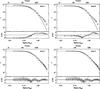 |
Fig. 5 Comparison between the azimuthally averaged y profile of the Coma cluster and various models. From left to right, top to bottom, we show the best-fit y models corresponding to the Arnaud et al. (2010) “universal” profile (A), the “universal” profile for merger systems (B), the modified “universal” profile (C, see 1), and the Vikhlinin et al. fitting formula (D, see. 2). For each panel we show in the Upper subpanel the points indicating the Coma y profile extracted in circular annuli centred at (RA, Dec) = (12h59m47s, + 27°55′53″). The plotted errors are the square root of the diagonal elements of the covariance matrix. Continuous and dotted lines are the best-fit projected y model after and before the convolution with the Planck PSF, respectively. The gray shaded region indicates the envelope derived from the 68.4% of models with the lowest χ2. In the lower subpanel we show the ratio between the observed and the best-fit model of the projected y profile in units of the relative error. The gray shaded region indicates the envelope derived from the 68.4% of models with the lowest χ2. |
Best-fit parameters for pressure model D Eq. (3) (Vikhlinin et al. 2006).
8. SZ-radio comparison
In Fig. 8 we overlay the y contour levels from Fig. 2 with the 352 MHz Westerbork Synthesis Radio Telescope diffuse total intensity image of the Coma cluster from Fig. 3 of Brown & Rudnick (2011). Most of the emission from compact radio sources both in and behind the cluster has been automatically subtracted. This image clearly shows a correlation between the diffuse radio emission and the y signal.
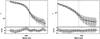 |
Fig. 6 Comparison between the projected y radial profile and the best-fit shock model of the west (left) and south-east (right) pressure jumps. Upper panels: the points indicate the Coma y profile extracted from the respective sectors, whose centres and position angles are reported in Table 3. The plotted errors are the square root of the diagonal elements of the covariance matrix. Continuous and dotted lines are the best-fit projected y model reported in Table 3 after and before the convolution with the Planck PSF, respectively. The two vertical lines mark the ± 1σ position range of the jump. The gray shaded region indicates the envelope derived from the 68.4% of models with the lowest χ2. Lower panels: ratio between the observed and the best-fit model of the projected y profile in units of the relative error. The gray shaded region indicates the envelope derived from the 68.4% of models with the lowest χ2. |
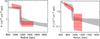 |
Fig. 7 68.4% confidence level range of the 3D-pressure model for the west (left panel) and south-east (right panel) sectors in Fig. 6. Grey shaded regions are the profiles derived from the Planck data. Red regions are the profiles derived from the XMM-Newton data. |
To provide a more quantitative comparison of the observed correlation, we first removed the remaining compact source emission in the radio image using the multiresolution filtering technique of Rudnick (2002). This removed 99.9% of the flux of unresolved sources, although residual emission likely associated with the tailed radio galaxy NGC 4874 blends in to the halo emission and contributes to the observed brightness within the central ~ 300 kpc. After filtering, we convolve the the diffuse radio emission to 10 arcmin resolution to match the Plancky map. We then extract the radio and y signals from the r < 50 arcmin region of the cluster and plot the results in Fig. 9. This is the first quantitative surface-brightness comparison of radio and SZ brightnesses2. We fit the data in the log–log plane using the Bayesian linear regression algorithm proposed by Kelly (2007), which accounts for errors in both abscissa and ordinate. The radio errors of 50 mJy/10′ beam are estimated from the off-source scatter, which is dominated by emission over several degree scales which is incompletely sampled by the interferometer. We find a quasi-linear relation between the radio emission and the y signal: 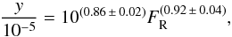 (7)where FR is the radio brightness in Jy beam-1 (10 arcmin beam FWHM).
Furthermore, using the same algorithm, we find that the intrinsic scatter between the two observables is only (9.6 ± 0.2)%. The quasi-linear relation between the radio emission and y signal, and its small scatter, are also clear from the good match of the radio and y profiles shown in Fig. 10, obtained by simply rescaling the 10′ FWHM convolved radio profile by 100.86 × 10⁵. An approximate linear relationship between the radio halo and SZ total powers for a sample of clusters was also found by Basu (2012), for the case that the signals are calculated over the volume of the radio halos.
There are several sources of scatter contributing to the point-by-point correlation in Fig. 9 and the radial radio profile in Fig. 10. First is the random noise in the measurements, which is ~2–3 mJy/135″ beam. Even after convolving to a 10 ′ beam, however, this is insignificant with respect to the other sources of scatter. A second issue is the proper zero-level of the radio map, based on the incomplete sampling of the largest scale structures by the interferometer. After making our best estimate of the zero-level correction, the remaining uncertainty is ~ 25 mJy/10′ beam, which is indicated as error bars in Fig. 10.
Note that the radio profile is significantly flatter at large radii than presented by Deiss et al. (1997). However, their image, made with the Effelsberg 100 m telescope at 1.4 GHz, appears to have set the zero level too high; they do not detect the faint Coma related emission mapped by Brown & Rudnick (2011) on the Green Bank Telescope, also at 1.4 GHz, and by Kronberg et al. (2007) at 0.4 GHz using Arecibo and DRAO. The addition of a zero level flux to the Deiss et al. (1997) measurements at their lowest contour level flattens out their profile to be consistent with ours at their furthest radial sample at 900 kpc.
Finally, there are azimuthal variations in the shape of the radial profile, both for the radio and Y images. This is seen most clearly in Fig. 6, comparing the west and southeast sectors. In the radio, the radial profiles in 90 degree wide sectors differ by up to a factor of 1.6 from the average; it is therefore important to understand Fig. 10 as an average profile, not one that applies universally at all azimuths. These azimuthal variations can also contribute to the scatter in the point-by-point correlation in Fig. 9, but only to the extent that the behavior differs between radio and Y.
9. Discussion
So far In this paper we have presented the data analysis of the Coma cluster observed in its SZ effect by the Planck satellite. In Sects. 5 and 6 we showed that, thanks to its great sensitivity, Planck is capable of detecting significant SZ emission above the zero level of the y map up to at least 4 Mpc which corresponds to R ≈ 3 × R500. This allows, for the first time, the study of the ICM pressure distribution in the outermost cluster regions. Furthermore, we performed a comparison with radio synchrotron emission. Here we discuss our results in more detail.
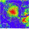 |
Fig. 8 Westerbork Synthesis Radio Telescope 352 MHz total intensity image of the Coma cluster from Fig. 3 of Brown & Rudnick (2011) overlaid with the y contour levels from Fig. 2. Most of the radio flux from compact sources has been subtracted; the resolution is 133 arcsec × 68 arcsec at − 1.5 degrees (W of N). The white circle indicates R500. |
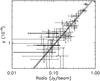 |
Fig. 9 Scatter plot between the radio map after smoothing to FWHM = 10′ and the y signal for the Coma cluster. To make the plot clearer, we show errors only for some points. |
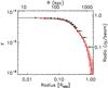 |
Fig. 10 Comparison of the y (black) and diffuse radio (red) global radio profiles in Coma. The radio profile has been convolved to 10 arcmin resolution to match the Planck FWHM and simply rescaled by the multiplication factor derived from the linear regression shown in Fig. 9. The radio errors are dominated by uncertainties in the zero level due to a weak bowling effect resulting from the lack of short interferometer spacings. |
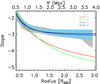 |
Fig. 11 Comparison of the pressure slopes of the best-fit models shown in Fig. 5. The red, green, blue and grey lines correspond to Models A, B, C, and D, respectively. |
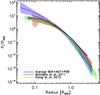 |
Fig. 12 Scaled Coma pressure profile with relative errors (black line and gray shaded region) overplotted on the scaled pressure profiles derived from numerical simulations of B04+N07+P08 (blue line and violet shaded region), Battaglia et al. (2012, red line and shaded region), and Dolag et al. (in prep., green line and light green shaded region). |
9.1. Global pressure profile
To study the 3D pressure distribution of the ICM up to r = 3 − 4 × R500, we fit the observed y profile using four analytic models summarised in Tables 1 and 2 (see Sect. 6).
From the ratio plot shown in Fig. 5 we immediately see that the “universal” pressure profile (Model A) is too steep both in the cluster centre and in the outskirts. The fit to the data thus results in an overestimation and underestimation of the observed SZ signal at smaller and larger radii, respectively. The overestimation of the observed profile at lower radii is consistent with WMAP (Komatsu et al. 2011). This is expected, since merging systems, such as Coma, have a flatter central pressure profile than the “universal” model (Arnaud et al. 2010). For merging systems, Model B should provide a better fit, as it has been specifically calibrated, at r < R500, to reproduce the average X-ray profiles of such systems (Arnaud et al. 2010). Figure 5 shows that this latter model indeed reproduces the data well at r < R500. Nevertheless, as for Model A, it still underestimates the observed y signal at larger radii. The observed profile clearly requires a shallower pressure profile in the cluster outskirts, as evident in Models C and D. This is important, as the external pressure slopes of both Model A and B are tuned to reproduce the mean slope predicted by the hydrodynamic simulations of Borgani et al. (2004), Nagai et al. (2007), and Piffaretti & Valdarnini (2008, from now on, B04+N07+P08). The Planck observation shows that the pressure slope for Coma is flatter than this value. This is also illustrated in Fig. 11 where we report the pressure slope as a function of the radius in our models: we find that while at R = 3 × R500 the mean predicted pressure slope is >4.5 for Models A and B, the observed pressure slope of Coma is ≈3.1 as seen in Model C and Model D.
In Fig. 12 we compare the scaled pressure profile of Coma with the pressure profiles derived from the numerical simulations of B04+N07+P08 and with the numerical simulations of Dolag et al. (in prep.) and Battaglia et al. (2012). We note that the simulations agree within their respective dispersions across the whole radial range. The Dolag et al. (in prep.) and Battaglia et al. (2012) profiles best agree within the central part, and are flatter than the B04+N07+P08 profile. This is likely due to the implementation of AGN feedback, which triggers energy injection at cluster centre, balancing radiative cooling and thus stopping the gas cooling. In the outer parts where cooling is negligible, the B04+N07+P08 and Dolag et al. (in prep.) profiles are in perfect agreement. The Battaglia et al. (2012) profile is slightly higher, but still compatible within its dispersion with the two other sets. Here again, differences are probably due to the specific implementation of the simulations.
We find that the Coma pressure profile at 2 × R500 is already 2 times higher than the average profile predicted by the B04+N07+P08 and Dolag et al. (in prep.) simulations, although still within the overall profile distribution which has quite a large scatter. The pressure profile of Battaglia et al. (2012) appears to be more consistent with the Coma profile and, in general, with the Planck SZ pressure profile obtained by stacking 62 nearby massive clusters (Planck Collaboration 2013). Still Fig. 12 indicates that the Coma pressure profile lies on the upper envelope of the pressure profile distribution derived from all the above simulations.
It is beyond the scope of this paper to discuss in detail the comparison between theoretical predictions. Here we just stress that, at such large radii, there is the possibility that the observed SZ signal could be significantly contaminated by SZ sources along the line of sight. This signal could be generated by: i) unresolved and undetected clusters; and ii) hot-warm gas filaments. Contamination would produce an apparent flattening of the pressure profile. We tested for possible contamination by unresolved clusters by re-extracting the y profile, excluding circular regions of r = 5′ centred on all NED identified clusters of galaxies present in the Coma cluster region. We find that the new y profile is consistent within the errors with the previous one, which implies that this kind of contamination is negligible in the Coma region. Thus, if there is SZ contamination it is probably related to the filamentary structures surrounding the cluster. We note that from the re-analysis of the ROSAT all-sky survey, Bonamente et al. (2009) and Bonamente et al. (2003) report the detection of extended soft X-ray emission in the Coma cluster region up to 5 Mpc from the cluster centre. They propose that this emission is related to filaments that converge toward Coma and is generated either by non-thermal radiation caused by accretion shocks or by thermal emission from the filaments themselves.
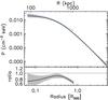 |
Fig. 13 Comparison between the Planck and XMM-Newton derived deprojected total pressure profiles. Upper panel: blue line and light blue shaded region are the deprojected pressure profile, with its 68.4% confidence level errors, obtained from the X-ray analysis of the XMM-Newton data (see text). The black line and grey shaded regions are the best-fit and 68.4% confidence level errors from the Model C pressure profile resulting from the fit shown in Fig. 5. Lower panel: ratio between the XMM-Newton and Planck derived pressure profiles. The black line and the grey shading indicate the best-fit and the 68.4% confidence level errors, respectively. |
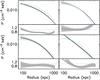 |
Fig. 14 Same as Fig. 13 but from profiles extracted in four 90deg sectors. From left to right, top to bottom we report the west (− 45deg,45deg), north (45deg,135deg), east (135deg,225deg) and south (225deg,3155deg) sectors, respectively. |
9.2. X-ray and SZ pressure profile comparison
We can compare the 3D pressure profile derived from the SZ observations to that obtained by multiplying the 3D electron density and the gas temperature profiles derived from the data analysis of the XMM-Newton mosaic of Coma.
In Fig. 13 we compare the 3D X-ray pressure profile with the 3D SZ profile of our reference Model C. We point the reader’s attention to the very large dynamical range shown in the figure: the radius extends up to r = 4 Mpc, probing approximately four orders of magnitude in pressure. In contrast, due to a combination of relatively high background level and available mosaic observations, XMM-Newton can probe the ICM pressure profile of Coma only up to ~ 1 Mpc. This is a four times smaller radius than Planck, probing only ~ one order of magnitude in pressure.
Due to the good statistics of both Planck and XMM-Newton data, we see that the pressure profile derived from Planck appears significantly lower than that of XMM-Newton, even if they differ by only 10–15%. This discrepancy may be related to the fact that we are applying spherical models to a cluster that has a much more complex morphology, with a number of substructures. A detailed structural analysis exploring these apparent pressure profile discrepancies is beyond the scope of this paper and will be presented in a forthcoming study. Here we just show a comparison of the 3D pressure profiles obtained from Planck and XMM-Newton in four 90deg sectors centred on the cluster and oriented towards the four cardinal points (see Fig. 14). This shows that the pressure discrepancy depends strongly on the sector considered. In particular, we find that while in the north sector the Planck and XMM-Newton pressure profiles agree within the errors, in the west sector we find discrepancies, up to 25−30%. As known from X-ray observations (see e.g., Neumann et al. 2003) the north sector is the one that is most regular, while the west sector is the one in which the ICM is strongly elongated, with the presence of major structures.
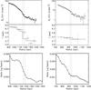 |
Fig. 15 Comparison of the X-ray and radio properties in the west (left panels) and south-east (right panels) sectors. Upper panels: surface brightness and temperature profiles of the XMM-Newton mosaic. The continuous histograms show the best-fit models. The 3D pressure model is overplotted in Fig. 7. Lower panels: radial profiles of 352 MHz radio emission at 2 arcmin resolution in the west (left) and south-east (right) sectors after subtraction of radio emission from compact sources (see Brown & Rudnick 2011). The two vertical lines mark the position range of the inferred jumps. |
9.3. Shocks
In Sect. 7 we show that Coma exhibits a localised steepening of its y profile in at least two directions, to the west and to the south-east. These suggest the presence of discontinuities in the underlying 3D pressure profile of the cluster. Using two sectors designed to follow the curvature of the y signal around the pressure jumps we estimate their amplitudes. This represents the first attempt to identify and estimate the amplitude of possible pressure jumps in the cluster atmosphere directly from the SZ signal. Interestingly, we find that similar features are observed at the same locations in the X-ray and radio bands.
In Fig. 15 we compare the X-ray and radio cluster properties from the west and south-east sectors selected from the SZ image. The X-ray surface brightness and temperature profiles have been derived from the XMM-Newton mosaic while the radio profile is extracted from the 352 MHz Westerbork observations at 2 arcmin resolution. To guide the reader’s eye, we mark, for each profile in the figure, the position of the pressure jump as derived from the analysis of the y signal (See Table 3). For both sectors we find that the X-ray surface brightness and radio profiles show relatively sharp features at the same position as the steepening of the Plancky profiles. This is also the case for the temperature profile of the west sector. For the south-east sector, however, this evidence is less clear. Because it is located in a much lower signal-to-noise region of the cluster, the error of the outermost temperature bin is too large to be able to put a stringent constraint on a possible temperature jump.
To check if the X-ray features are also consistent with the hypothesized presence of a discontinuity in the cluster pressure profile we simultaneously fit the observed X-ray surface brightness and temperature profiles using the following discontinuous 3D density and temperature models: 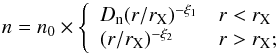 (8)and
  (9)Here rX is the position of the X-ray jump and Dn and DT are amplitudes of the density and temperature discontinuities, respectively. The above models are projected along the line of sight for r < 10 Mpc using a temperature function appropriate for spectroscopic data (Mazzotta et al. 2004). Notice that due to the poor statistics of the temperature in the south-east sector, for this profile we fix ξ1 = ξ1 = 0. This choice does not affect the determination of the jump position rX which is mainly driven by the surface brightness rather than by the temperature profile.
The best-fit position, density, and temperature jumps, together with their 68.4% confidence level errors are reported in Table 4. To make a direct comparison with the pressure jump measured from the SZ signal, in the same table we add the amplitude of the X-ray pressure jump derived by multiplying the X-ray density and temperature models (i.e., Px = nekT).
The best-fit surface brightness and projected temperature models are shown as histograms in Fig. 15. The best-fit 3D Px model and its 68.4% confidence level errors are overlaid in Fig. 7.
From Table 4 we see that the X-ray data from the west sector are consistent with the presence of a discontinuity, both in the 3D density and 3D temperature profiles. Both jumps are detected at >5σ confidence and the pressure jumps derived from X-ray and from SZ are consistent within the 68.4% confidence level errors (Table 3 and Table 4 ). This agreement near the discontinuity is also seen in Fig. 7 which, in addition, shows that the 3D pressure profiles for the west sector derived from the SZ and the X-ray data are consistent not only near the jump, but also over a much wider radial range.
These results indicate that the feature seen by Planck is produced by a shock induced by supersonic motions in the cluster’s hot gas atmosphere. Assuming Rankine-Hugoniot pressure jump conditions across the fronts (Sect. 85 of Landau & Lifshitz 1959), the discontinuity in the density, temperature and pressure profiles are uniquely linked to the shock Mach number.
Table 4 shows that the Mach number obtained from the SZ and X-ray pressure profiles are also consistent within the ±1σ confidence level errors. Furthermore, the Mach number derived from the X-ray density and temperature profiles agree within the ±2σ confidence level errors. This agreement supports the hypothesis that the west feature observed by Planck is a shock front.
For the south-east sector Table 4 shows that the X-ray surface brightness profile is consistent with the presence of a significant discontinuity in the 3D density profile. Due to the modest statistics, the temperature model returns large errors and DT is not constrained (see Table 4). Thus, although consistent, we cannot confirm the presence of a temperature jump. Despite this we find that, as for the west sector, the pressure jumps and the pressure profiles derived from X-ray and from SZ are consistent within the 68.4% confidence level errors (see Fig. 7 and Tables 3 and 4). Finally, Table 4 shows that the Mach numbers derived from the amplitudes of the different 3D models are all consistent within the 68.4% uncertainty levels. We would like to stress that this is true not only for MT and MnT which, being directly connected to DT, have relatively large errors, but also for Mn and MSZ which do not depends on DT at all. As for the west sector, this agreement supports the initial hypothesis that the south-east feature observed by Planck is also a shock front.
Notice that the good agreement between the 3D pressure models derived from the X-ray and SZ data, both in the west and south-east sectors, indicate that, within the selected regions, spherical symmetry is a good approximation to the underlying pressure distribution.
We conclude this section by pointing the reader’s attention to the fact that, even though the radio and X-ray observations have a much better PSF than Planck, Fig. 15 shows that the respective jumps in these observations appear smooth on a scale of ≈200 kpc ≈ 7′. As explained in detail in Appendix A this is simply a projection effect (see also Fig. 7 and Sect. 7). Despite its relatively large PSF, Planck is able to measure pressure jumps in the atmosphere of the Coma cluster.
9.4. Quasi-linear SZ-radio relation
In Sect. 8 we show that for the Coma cluster the radio brightness and y emission scale approximately linearly with a small scatter between the radio emission and thermal pressure. Due to the near-linear correlation, where line-of-sight projection effects cancel out, we work here with volume-averaged emissivities. We first express the monochromatic radio emissivity [erg s-1 cm-3 sr-1 Hz-1] as:  (10)where α is the spectral index,B is the magnetic field, BCMB ≈ 3(1 + z) μ G is the equivalent magnetic field of the CMB, and nCRe and
  are the density and injection rate of cosmic-ray electrons (CRe) , respectively. In general, can be a function of position and electron energy, and will depend on the model of cosmic-ray acceleration assumed. In secondary (hadronic) acceleration models (Dennison 1980; Vestrand 1982), the relativistic electrons are produced in collisions of long-lived cosmic ray protons with the thermal electrons, resulting in
  , where nCRp and ne is the density of cosmic-ray protons and thermal electrons, respectively. Recent models in this category (Keshet & Loeb 2010; Keshet et al. 2010) require that, in contrast to ne, nCRp should be constant over the cluster volume in order to match the cluster radio brightness profiles. Pfrommer et al. (2008) show that there is strong cosmic-ray proton injection even in the cluster peripheries, due to the stronger shock waves there. Strong radio cosmic-ray proton diffusion and streaming within the ICM could also lead to a completely flat cosmic-ray proton profile (Enßlin et al. 2011). In the limit where B ≫ BCMB and assuming α ≈ 1 (e.g. Giovannini et al. 1993; Deiss et al. 1997), this would lead to ϵr ∝ ne ∝ y/T. This is consistent with our observations3, especially since ne(r) varies much more than T(r) in the Coma cluster (see e.g. Arnaud et al. 2001; Snowden et al. 2008). Jeltema & Profumo (2011) derive a lower limit for the average field in Coma of 1.7 μG, from limits on the Fermi γ-ray flux. The γ-ray analysis thus leaves open the question of whether Coma could be in the strong-field limit.
However, the rotation measure observations of Bonafede et al. (2010) provide characteristic values of 4–5 μG for the combined contributions of the central diffuse cluster field and contributions local to each radio source (e.g. Guidetti et al. 2011; Rudnick & Blundell 2003). The majority of Coma’s volume, which is outside of the cluster core, is thus in the weak-field limit, which leads to ϵr ∝ y B2/T. To remain consistent with the linear correlation found here, the magnetic field would thus need to be nearly independent of thermal density. The non-ideal MHD simulations of Bonafede et al. (2011) show a typical scaling of  , which would yield ϵr ∝ y2.2/T2.2. This could make the secondary model inconsistent with the observations in the weak-field limit.
Primary (re-)acceleration models assume that relativistic electrons are accelerated directly from shocks and/or turbulence generated in cluster mergers. The turbulent re-acceleration model (Schlickeiser et al. 1987; Brunetti et al. 2001; Petrosian 2001) leads to a scaling of ϵr ∝ ne in the B < BCMB limit (Cassano et al. 2007) if one assumes B2 ∝ ne which is close to the simulation scaling results of Bonafede et al. (2011). Such a scaling relation is consistent with the observed correlation. However, in order to connect the cosmic-ray electron density to ne, primary models depend on a large number of free parameters, which are generally fit to match the observations. Recent attempts to reduce the number of assumptions by introducing secondary cosmic ray electrons and protons as seed particles (Brunetti & Lazarian 2011, see above) fail to reproduce the linear correlation in the weak-field limit. This is another manifestation of the problem all simple models have in explaining the large extent of cluster radio profiles when compared to the X-rays and inferred magnetic fields (e.g., Dolag & Enßlin 2000; Govoni et al. 2001; Donnert et al. 2010; Brown & Rudnick 2011). In future, robust measurements of the cluster’s magnetic field profile, coupled with high-resolution radio/X-ray/SZ correlations, will be needed to rule out these naive models.
9.5. Pressure jumps and radio emission
Shocks play an important role in the production of radio emission. We expect that shocks created during cluster mergers will compress magnetic fields and accelerate relativistic particles. However, the radiating electrons will quickly lose their energy post-shock, and may not be visible for more than ~ 100 kpc behind the shock (e.g., Markevitch et al. 2005), given characteristic shock velocities and magnetic fields at μ G levels. These shock-accelerated electrons, in shock-compressed magnetic fields, have been proposed as the explanation for the observed polarised radio synchrotron radiation from cluster peripheral relic sources (Ensslin et al. 1998). Lower fields do not increase the electron lifetimes, and can even decrease them at fixed observing frequency, because of inverse Compton losses against the CMB. Recent simulations show that the presence of cluster-wide turbulence following a major merger is maintained for a few Gyr at a few percent thermal pressure (e.g., Dolag et al. 2005; Vazza et al. 2006; Kang et al. 2007; Paul et al. 2011). This turbulence can re-accelerate mildly relativistic seed electrons, and is potentially responsible for the large-scale halo emission (see above). In addition, an extensive population of low Mach number shocks is also seen in simulations (e.g., Miniati et al. 2000; Pfrommer et al. 2006) and could play an important role in particle re-acceleration.
Shocks will also induce turbulence in the post-shock region (~200–300 kpc). There are hints from the small-scale X-ray residuals (Fig. 3 of Schuecker et al. 2004) that such turbulence may exist interior to the possible shocks seen in the west and south-east. For the western region, the combination of the SZ/X-ray pressure jump, X-ray suggested turbulence, and excess synchrotron emission, points toward a connection between turbulence and diffuse synchrotron emission. The details of that connection, however, are not clear. In addition to direct acceleration by turbulence, the post-shock synchrotron emission could be a result of a population of weaker, as yet undetected shocks, or freshly accelerated cosmic-ray protons interacting with the ICM in a region where turbulence has amplified the magnetic field (e.g., Dolag et al. 2005; Ryu et al. 2008; Kushnir et al. 2009; Keshet 2010). Synchrotron spectral indices and magnetic field measurements, in combination with reliable measurements of weaker shocks and turbulence, would be needed to discriminate between potential models.
The expected rapid loss of radio emissivity post-shock can also help us understand why shocks are sometimes easily detected in the radio, but other times are not. In the clearest cases, radio shocks are seen beyond any central halo as relatively thin structures known as “peripheral relics” (van Weeren et al. 2010), where they can accelerate relativistic electrons. Radio shocks may also be found at or near the edge of the halo, and would be characterised by a sharp, but low contrast, rise in brightness, while the post-shock emission blends in with the halo instead of falling off. The western shock described here in Coma, as well as suggested shocks at the edges of halos in Abell clusters 521 and 754 (Giacintucci et al. 2008; Markevitch 2010; Macario et al. 2011) are likely examples of this case. Contrast effects will camouflage the appearance of shocks that are projected against any radio halo emission. This is probably the case for the y shock in the south-east, where the radio halo extends far beyond the shock. The Coma cluster thus hosts all three types of “radio shocks”: a) the classic peripheral relicat a distance of 1.7 Mpc from the centre (which Ensslin et al. 1998 and Brown & Rudnick 2011 suggest is an “infall" shock); b) the western shock at the edge of the halo; and c) the south-east shock projected against the fading radio halo.
10. Conclusions
We present the SZ observations of the Coma cluster based on the Planck nominal survey of 14 months. The excellent sensitivity of Planck allows, for the first time, the detection of SZ emission out to at least R ≈ 3 × R500. We limit our investigation to the radial and sectoral properties of the ICM, and we study the pressure distribution to the outermost cluster regions. Our three main results can be summarised as follows:
-
the Coma pressure profile is flatter than the mean pressure profilepredicted by the B04+N07+P08 numerical simulations and lieson the upper envelope of the simulated profile distribution. Thiseffect has also been found in the pressure profile derived bystacking 62 nearby clusters of galaxies observed withPlanck (PlanckCollaboration 2013).
-
Planck detects a localised steepening of the y profile about half a degree to the west and also to the south-east of the cluster centre. Features in the X-ray and radio synchrotron profiles at similar locations suggest the presence of shock waves that propagate with Mach number
 and
and  in the west and south-east directions, respectively.
 -
the y and radio-synchrotron signals are quasi-linearly correlated on Mpc-scales with only small intrinsic scatter. This implies either that, unlike the thermal plasma, the energy density of cosmic-ray electrons is relatively constant throughout the cluster, or that the magnetic fields fall off much more slowly with radius than previously thought. We detect a correspondence between the western y shock and a previously reported radio/X-ray edge, and we argue that either the magnetic fields are strong in the cluster outskirts, which would permit the hadronic model to explain the radio emission, or some sort of re-acceleration by turbulence or additional shock waves must operate in the region behind the detected outer shock structures.
Even though this analysis is based on only about half of the data collected by Planck, our results represent a substantial step forward in the study of the physics of the Coma cluster. The full set of data collected by Planck, will not only improve the signal-to-noise by another factor ~ but also significantly improve our understanding of instrumental effects. Thus, we will be able to generate more accurate y maps, and more thoroughly unveil Coma’s two-dimensional SZ structure and its filamentary environment.
Planck (http://www.esa.int/planck) is a project of the European Space Agency (ESA) with instruments provided by two scientific consortia funded by ESA member states (in particular the lead countries: France and Italy) with contributions from NASA (USA), and telescope reflectors provided in a collaboration between ESA and a scientific consortium led and funded by Denmark.
See e.g. Ferrari et al. (2011) and Malu & Subrahmanyan (2012) for a morphological comparison between radio and SZ brightnesses.
In the case that α = 1 + δ, the relationship would be ϵr ∝ (y/T)1 + δ/2, if we assume  . E.g., if we use α = 1.2 (Giovannini et al. 1993), we would expect
  , which is approximately our measured value. However, we continue to use the term “linear relationship”, with the understanding that the difference between our measured slope and linearity is consistent for our simple assumption about the spectral index.
Acknowledgments
A description of the Planck Collaboration and a list of its members, indicating which technical or scientific activities they have been involved in, can be found at http://www.rssd.esa.int/Planck_Collaboration. The Planck Collaboration acknowledges the support of: ESA; CNES and CNRS/INSU-IN2P3-INP (France); ASI, CNR, and INAF (Italy); NASA and DoE (USA); STFC and UKSA (UK); CSIC, MICINN and JA (Spain); Tekes, AoF and CSC (Finland); DLR and MPG (Germany); CSA (Canada); DTU Space (Denmark); SER/SSO (Switzerland); RCN (Norway); SFI (Ireland); FCT/MCTES (Portugal); and DEISA (EU). Partial support for this work for L. Rudnick comes from U.S. NSF Grant 09-08668 to the University of Minnesota. We would also like to acknowledge useful conversations with G. Brunetti.
References
- Arnaud, M., Aghanim, N., Gastaud, R., et al. 2001, A&A, 365, L67 [NASA ADS] [CrossRef] [EDP Sciences] [Google Scholar]
- Arnaud, M., Pratt, G. W., Piffaretti, R., et al. 2010, A&A, 517, A92 [NASA ADS] [CrossRef] [EDP Sciences] [Google Scholar]
- Basu, K. 2012, MNRAS, 421, L112 [NASA ADS] [CrossRef] [Google Scholar]
- Battaglia, N., Bond, J. R., Pfrommer, C., & Sievers, J. L. 2012, ApJ, 758, 74 [NASA ADS] [CrossRef] [Google Scholar]
- Bersanelli, M., Mandolesi, N., Butler, R. C., et al. 2010, A&A, 520, A4 [NASA ADS] [CrossRef] [EDP Sciences] [Google Scholar]
- Bobin, J., Moudden, Y., Starck, J.-L., Fadili, J., & Aghanim, N. 2008, Stat. Methodol., 5, 307 [NASA ADS] [CrossRef] [Google Scholar]
- Bonafede, A., Feretti, L., Murgia, M., et al. 2010, A&A, 513, A30 [NASA ADS] [CrossRef] [EDP Sciences] [Google Scholar]
- Bonafede, A., Dolag, K., Stasyszyn, F., Murante, G., & Borgani, S. 2011, MNRAS, 418, 2234 [NASA ADS] [CrossRef] [Google Scholar]
- Bonamente, M., Joy, M. K., & Lieu, R. 2003, ApJ, 585, 722 [NASA ADS] [CrossRef] [Google Scholar]
- Bonamente, M., Lieu, R., & Bulbul, E. 2009, ApJ, 696, 1886 [NASA ADS] [CrossRef] [Google Scholar]
- Borgani, S., Murante, G., Springel, V., et al. 2004, MNRAS, 348, 1078 [NASA ADS] [CrossRef] [Google Scholar]
- Bourdin, H., & Mazzotta, P. 2008, A&A, 479, 307 [NASA ADS] [CrossRef] [EDP Sciences] [Google Scholar]
- Bourdin, H., Arnaud, M., Mazzotta, P., et al. 2011, A&A, 527, A21 [NASA ADS] [CrossRef] [EDP Sciences] [Google Scholar]
- Briel, U. G., Henry, J. P., & Boehringer, H. 1992, A&A, 259, L31 [NASA ADS] [Google Scholar]
- Brown, S., & Rudnick, L. 2011, MNRAS, 412, 2 [NASA ADS] [CrossRef] [Google Scholar]
- Brunetti, G., & Lazarian, A. 2011, MNRAS, 410, 127 [NASA ADS] [CrossRef] [Google Scholar]
- Brunetti, G., Setti, G., Feretti, L., & Giovannini, G. 2001, MNRAS, 320, 365 [NASA ADS] [CrossRef] [Google Scholar]
- Cassano, R., Brunetti, G., Setti, G., Govoni, F., & Dolag, K. 2007, MNRAS, 378, 1565 [NASA ADS] [CrossRef] [Google Scholar]
- Churazov, E., Vikhlinin, A., Zhuravleva, I., et al. 2012, MNRAS, 2290 [Google Scholar]
- De Petris, M., D’Alba, L., Lamagna, L., et al. 2002, ApJ, 574, L119 [NASA ADS] [CrossRef] [Google Scholar]
- Deiss, B. M., Reich, W., Lesch, H., & Wielebinski, R. 1997, A&A, 321, 55 [NASA ADS] [Google Scholar]
- Dennison, B. 1980, ApJ, 239, L93 [NASA ADS] [CrossRef] [Google Scholar]
- Dolag, K., & Enßlin, T. A. 2000, A&A, 362, 151 [NASA ADS] [Google Scholar]
- Dolag, K., Vazza, F., Brunetti, G., & Tormen, G. 2005, MNRAS, 364, 753 [NASA ADS] [CrossRef] [Google Scholar]
- Donnert, J., Dolag, K., Cassano, R., & Brunetti, G. 2010, MNRAS, 407, 1565 [NASA ADS] [CrossRef] [Google Scholar]
- Dow, K. L., & White, S. D. M. 1995, ApJ, 439, 113 [NASA ADS] [CrossRef] [Google Scholar]
- Ensslin, T. A., Biermann, P. L., Klein, U., & Kohle, S. 1998, A&A, 332, 395 [NASA ADS] [Google Scholar]
- Enßlin, T., Pfrommer, C., Miniati, F., & Subramanian, K. 2011, A&A, 527, A99 [NASA ADS] [CrossRef] [EDP Sciences] [Google Scholar]
- Eriksen, H. K., Banday, A. J., Górski, K. M., & Lilje, P. B. 2004, ApJ, 612, 633 [NASA ADS] [CrossRef] [Google Scholar]
- Ferrari, C., Intema, H. T., Orrù, E., et al. 2011, A&A, 534, L12 [NASA ADS] [CrossRef] [EDP Sciences] [Google Scholar]
- Giacintucci, S., Venturi, T., Macario, G., et al. 2008, A&A, 486, 347 [NASA ADS] [CrossRef] [EDP Sciences] [Google Scholar]
- Giovannini, G., Feretti, L., Venturi, T., Kim, K.-T., & Kronberg, P. P. 1993, ApJ, 406, 399 [NASA ADS] [CrossRef] [Google Scholar]
- Górski, K. M., Hivon, E., Banday, A. J., et al. 2005, ApJ, 622, 759 [NASA ADS] [CrossRef] [Google Scholar]
- Govoni, F., Enßlin, T. A., Feretti, L., & Giovannini, G. 2001, A&A, 369, 441 [NASA ADS] [CrossRef] [EDP Sciences] [Google Scholar]
- Guidetti, D., Laing, R. A., Bridle, A. H., Parma, P., & Gregorini, L. 2011, MNRAS, 413, 2525 [NASA ADS] [CrossRef] [Google Scholar]
- Herbig, T., Readhead, A. C. S., & Lawrence, C. R. 1992, in BAAS Meeting Abstracts, 24, 1263 [Google Scholar]
- Herbig, T., Lawrence, C. R., Readhead, A. C. S., & Gulkis, S. 1995, ApJ, 449, L5 [NASA ADS] [CrossRef] [Google Scholar]
- Hurier, G., Hildebrandt, S. R., & Macias-Perez, J. F. 2010, unpublished [arXiv:1007.1149] [Google Scholar]
- Jeltema, T. E., & Profumo, S. 2011, ApJ, 728, 53 [NASA ADS] [CrossRef] [Google Scholar]
- Kang, H., Ryu, D., Cen, R., & Ostriker, J. P. 2007, ApJ, 669, 729 [NASA ADS] [CrossRef] [Google Scholar]
- Kelly, B. C. 2007, ApJ, 665, 1489 [NASA ADS] [CrossRef] [Google Scholar]
- Keshet, U. 2010, unpublished [arXiv:1011.0729] [Google Scholar]
- Keshet, U., & Loeb, A. 2010, ApJ, 722, 737 [NASA ADS] [CrossRef] [Google Scholar]
- Keshet, U., Markevitch, M., Birnboim, Y., & Loeb, A. 2010, ApJ, 719, L74 [NASA ADS] [CrossRef] [Google Scholar]
- Komatsu, E., Smith, K. M., Dunkley, J., et al. 2011, ApJS, 192, 18 [NASA ADS] [CrossRef] [Google Scholar]
- Kronberg, P. P., Kothes, R., Salter, C. J., & Perillat, P. 2007, ApJ, 659, 267 [NASA ADS] [CrossRef] [Google Scholar]
- Kushnir, D., Katz, B., & Waxman, E. 2009, Cosmol. Astropart. Phys., 9, 24 [Google Scholar]
- Lamarre, J., Puget, J., Ade, P. A. R., et al. 2010, A&A, 520, A9 [NASA ADS] [CrossRef] [EDP Sciences] [Google Scholar]
- Lancaster, K., Genova-Santos, R., Falcòn, N., et al. 2005, MNRAS, 359, 16 [NASA ADS] [CrossRef] [Google Scholar]
- Landau, L. D., & Lifshitz, E. M. 1959, Fluid Mechanics (England: Pergamon Press Oxford) [Google Scholar]
- Leahy, J. P., Bersanelli, M., D’Arcangelo, O., et al. 2010, A&A, 520, A8 [NASA ADS] [CrossRef] [EDP Sciences] [Google Scholar]
- Macario, G., Markevitch, M., Giacintucci, S., et al. 2011, ApJ, 728, 82 [NASA ADS] [CrossRef] [Google Scholar]
- Malu, S. S., & Subrahmanyan, R. 2012, J. Astrophys. Astron., 20 [Google Scholar]
- Mandolesi, N., Bersanelli, M., Butler, R. C., et al. 2010, A&A, 520, A3 [Google Scholar]
- Markevitch, M. 2010 [arXiv:1010.3660] [Google Scholar]
- Markevitch, M., Govoni, F., Brunetti, G., & Jerius, D. 2005, ApJ, 627, 733 [NASA ADS] [CrossRef] [Google Scholar]
- Mazzotta, P., Rasia, E., Moscardini, L., & Tormen, G. 2004, MNRAS, 354, 10 [NASA ADS] [CrossRef] [Google Scholar]
- Meneghetti, M., Rasia, E., Merten, J., et al. 2010, A&A, 514, A93 [NASA ADS] [CrossRef] [EDP Sciences] [Google Scholar]
- Mennella, A., Butler, R. C., Curto, A., et al. 2011, A&A, 536, A3 [NASA ADS] [CrossRef] [EDP Sciences] [Google Scholar]
- Miniati, F., Ryu, D., Kang, H., et al. 2000, ApJ, 542, 608 [NASA ADS] [CrossRef] [Google Scholar]
- Nagai, D., Vikhlinin, A., & Kravtsov, A. V. 2007, ApJ, 655, 98 [NASA ADS] [CrossRef] [Google Scholar]
- Neumann, D. M., Arnaud, M., Gastaud, R., et al. 2001, A&A, 365, L74 [NASA ADS] [CrossRef] [EDP Sciences] [Google Scholar]
- Neumann, D. M., Lumb, D. H., Pratt, G. W., & Briel, U. G. 2003, A&A, 400, 811 [NASA ADS] [CrossRef] [EDP Sciences] [Google Scholar]
- Paul, S., Iapichino, L., Miniati, F., Bagchi, J., & Mannheim, K. 2011, ApJ, 726, 17 [NASA ADS] [CrossRef] [Google Scholar]
- Petrosian, V. 2001, ApJ, 557, 560 [NASA ADS] [CrossRef] [Google Scholar]
- Pfrommer, C., Springel, V., Enßlin, T. A., & Jubelgas, M. 2006, MNRAS, 367, 113 [NASA ADS] [CrossRef] [Google Scholar]
- Pfrommer, C., Enßlin, T. A., & Springel, V. 2008, MNRAS, 385, 1211 [NASA ADS] [CrossRef] [Google Scholar]
- Piffaretti, R., & Valdarnini, R. 2008, A&A, 491, 71 [NASA ADS] [CrossRef] [EDP Sciences] [Google Scholar]
- Planck Collaboration 2011a, A&A, 536, A1 [NASA ADS] [CrossRef] [EDP Sciences] [Google Scholar]
- Planck Collaboration 2011b, A&A, 536, A2 [NASA ADS] [CrossRef] [EDP Sciences] [Google Scholar]
- Planck Collaboration 2011c, A&A, 536, A9 [NASA ADS] [CrossRef] [EDP Sciences] [Google Scholar]
- Planck Collaboration 2011d, A&A, 536, A8 [NASA ADS] [CrossRef] [EDP Sciences] [Google Scholar]
- Planck Collaboration 2011e, A&A, 536, A10 [NASA ADS] [CrossRef] [EDP Sciences] [Google Scholar]
- Planck Collaboration 2013, A&A, 550, A131 [NASA ADS] [CrossRef] [EDP Sciences] [Google Scholar]
- Planck HFI Core Team 2011a, A&A, 536, A4 [NASA ADS] [CrossRef] [EDP Sciences] [Google Scholar]
- Planck HFI Core Team 2011b, A&A, 536, A6 [NASA ADS] [CrossRef] [EDP Sciences] [Google Scholar]
- Remazeilles, M., Delabrouille, J., & Cardoso, J.-F. 2011, MNRAS, 410, 2481 [NASA ADS] [CrossRef] [Google Scholar]
- Rosset, C., Tristram, M., Ponthieu, N., et al. 2010, A&A, 520, A13 [NASA ADS] [CrossRef] [EDP Sciences] [Google Scholar]
- Rudnick, L. 2002, PASP, 114, 427 [NASA ADS] [CrossRef] [Google Scholar]
- Rudnick, L., & Blundell, K. M. 2003, ApJ, 588, 143 [NASA ADS] [CrossRef] [Google Scholar]
- Ryu, D., Kang, H., Cho, J., & Das, S. 2008, Science, 320, 909 [NASA ADS] [CrossRef] [PubMed] [Google Scholar]
- Sarazin, C. L. 1999, ApJ, 520, 529 [NASA ADS] [CrossRef] [Google Scholar]
- Schlickeiser, R., Sievers, A., & Thiemann, H. 1987, A&A, 182, 21 [NASA ADS] [Google Scholar]
- Schuecker, P., Finoguenov, A., Miniati, F., Böhringer, H., & Briel, U. G. 2004, A&A, 426, 387 [NASA ADS] [CrossRef] [EDP Sciences] [Google Scholar]
- Silverberg, R. F., Cheng, E. S., Cottingham, D. A., et al. 1997, ApJ, 485, 22 [NASA ADS] [CrossRef] [Google Scholar]
- Snowden, S. L., Mushotzky, R. F., Kuntz, K. D., & Davis, D. S. 2008, A&A, 478, 615 [NASA ADS] [CrossRef] [EDP Sciences] [Google Scholar]
- Tauber, J. A., Mandolesi, N., Puget, J., et al. 2010, A&A, 520, A1 [NASA ADS] [CrossRef] [EDP Sciences] [Google Scholar]
- van Weeren, R. J., Röttgering, H. J. A., Brüggen, M., & Hoeft, M. 2010, Science, 330, 347 [NASA ADS] [CrossRef] [PubMed] [Google Scholar]
- Vazza, F., Tormen, G., Cassano, R., Brunetti, G., & Dolag, K. 2006, MNRAS, 369, L14 [NASA ADS] [Google Scholar]
- Vestrand, W. T. 1982, AJ, 87, 1266 [NASA ADS] [CrossRef] [Google Scholar]
- Vikhlinin, A., Forman, W., & Jones, C. 1997, ApJ, 474, L7 [NASA ADS] [CrossRef] [Google Scholar]
- Vikhlinin, A., Kravtsov, A., Forman, W., et al. 2006, ApJ, 640, 691 [NASA ADS] [CrossRef] [Google Scholar]
- White, S. D. M., Briel, U. G., & Henry, J. P. 1993, MNRAS, 261, L8 [NASA ADS] [CrossRef] [Google Scholar]
- Zacchei, A., Maino, D., Baccigalupi, C., et al. 2011, A&A, 536, A5 [NASA ADS] [CrossRef] [EDP Sciences] [Google Scholar]
Appendix A: Pressure profile discontinuities as seen by Planck
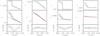 |
Fig. A.1 Histogram of the effects of projection and Planck PSF on the y radial profile produced by an underlying broken power law pressure profile with and without a pressure discontinuity. In this figure we fix P0 = 10. × 10-4 cm-3 keV, rJ = 1.1 Mpc and, from left to right we consider four different cases: i) η1 = 0 , η2 = 2, DJ = 4; ii) η1 = 0 , η2 = 2, DJ = 1; iii) η1 = 2 , η2 = 0, DJ = 4; and iv) η1 = 2 , η2 = 0, DJ = 1. Upper panels: the underlying 3D pressure profile. Middle panels: the black and red histograms are the projected y profiles observed by an instrument with infinite angular resolution and with a PSF of 10 arcmin, respectively. The red line represents the best-fit of a simple power law to the entire convolved profile (red histogram). The black line is the same as the red line, but considering only the three outermost projected profile bins. Lower panels: ratio between the PSF-convolved and projected y profile and its best-fit power law model (red histogram and lines in middle panel) in units of a relative error, which, for this illustration, we set to 10%. |
In this section we show that the 10 arcmin angular resolution of Planck is still sufficient to detect and measure 3D pressure jump features in the Coma cluster. This is because at the cluster redshift, 10 arcmin ≈ 280 kpc, which is of the order of the smoothing induced by projection. To show this, we assume a discontinuous 3D pressure profile described by Eq. (6). We project this profile along the line of sight and we calculate the corresponding y profile as observed with an instrument with:
-
i)
infinite angular resolution;
-
ii)
a 10′ FWHM angular resolution, as for Planck.
The results of this exercise are illustrated in Fig. A.1, where we compare four different cases with and without pressure jumps. In the upper section of each panel of Fig. A.1 we show the input 3D pressure profiles. In the middle sections we show the projected pressure profiles without any smoothing (as black histograms). The lower sections show deviations from a single power law fit. The panel on the left shows that, due to simple projection effects, the y profile appears smoothed with an equivalent smoothing scale of ≈200–250 kpc. For Coma, this corresponds to an angular scale of 7–9 arcmin. In the same panel we overplot, as a red histogram, the y profile convolved with the Planck PSF. This illustrates that the effect of the PSF smoothing is secondary with respect to projection effects. This indicates that there is only a modest gain, from the detection point of view, in observing this specific feature using an instrument with a much better angular resolution than Planck. Notice that the fact that the projection of the 3D pressure distribution onto a plane converts the sharp jump into a curved surface brightness profile allows us to recover the position of rJ with an accuracy higher than the angular resolution of Planck.
Figure A.2 clearly shows that the range of radii affected by the rJ value is of the order of rJ itself. Since rJ > 10′, many independent data points with large signal-to-noise ratio are contributing to the determination of rJ, driving the uncertainty well below the nominal angular resolution of the telescope. Of course the value of rJ is still subject to systematic uncertainties, e.g. from our assumption of spherical symmetry.
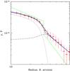 |
Fig. A.2 Comparison of the 3D pressure model (green line) and the corresponding projected y profile, smoothed with the 10′ beam. The dotted black line shows the expected y profile due to the inner power component, while the dashed line shows the contribution of the outer power law component. The black solid line is the sum of these two components. For comparison, the blue line shows the same model, but not convolved with the 10′ beam. In this plot rJ ~ 30′. Due to projection effects, the range of radii affected by the value of rJ is of order rJ itself. Since rJ exceeds 10′, many independent data points with large signal-to-noise ratio contributes to the determination of rJ, allowing rJ to be estimated with an uncertainty below the nominal angular resolution of the telescope. |
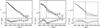 |
Fig. A.3 Results of the fit of the y profile extracted from three cluster sectors with a simple power law. Left panel: sector with the same angular size and extension as the west shock but pointing to the north, where there are no visible shock features. Middle panel: profile of the west shock. Right panel: profile of the south-east shock. In the lower panel of each figure we report the ratio between the observed and the best-fit model of the projected y profile in units of the relative error. The figure clearly illustrates that while the power law gives a good fit for the north sector where no shock is present, it returns a poor fit in the west and south-east sectors. These two cluster regions require a discontinuity in the pressure jump, as shown in Fig. 6. |
We use the above exercise to illustrate two practical ways to identify the presence of a possible underlying 3D discontinuous pressure profile, hidden behind some observed projected profile extracted in a specific cluster sector. The first way is to search for the actual pressure jump in the observed pressure profile. As projection smooths the profile, this needs to be done by looking at the profile extremes. We first notice that the outermost bins of the profile are practically unaffected by PSF smoothing. This is clear in the middle sections of Fig. A.1, where the red and back histograms are similar in the outermost 3 or 4 bins. At this point, if we fit a line to either the 3 or 4 outermost bins, this will give an indication of the un-convolved y profile slope at large radii. If we extrapolate this line to the centre, we can easily highlight the presence of a pressure jump. This procedure is shown in the middle section of Fig. A.1, using black straight lines. From Fig. A.1 we can see that this procedure highlights the intensity variation due to a pressure jump (see first and third panels). In the case where we have no pressure jump (second and forth panels) the best-fit line to the outermost bins tends to closely follow the entire profile.
The second way to highlight the presence of a pressure jump is to fit a line to the entire observed profile and to examine the residuals. This procedure is illustrated in the middle and lower sections of Fig. A.1. The red lines in the middle section are the best-fit power law relations to the entire observed profile (red histogram). The crosses in the lower panels indicate the differences, in units of the relative errors, between the PSF convolved projected y profile and its best-fit power law model. This figure shows that a 3D pressure jump induces a characteristic signature in the residuals.
In Fig. A.3 we apply this second technique to the Coma cluster by showing the fit of the y profile extracted from three cluster sectors with a simple power law. The figure clearly illustrates that while the power law gives a good fit for the north sector where no shock is present, it returns a poor fit in the west and south-east sectors. These two cluster regions require a discontinuity in the pressure jump, as shown in Fig. 6.
All Tables
Best-fit parameters for the Arnaud et al. (2010) pressure model Eqs. (4) and (5).
All Figures
|
Fig. 1 Upper panel: radial profile of y in a set of circular annuli centred on Coma. The blue curve is the best fitting simple model to the profile over the radial range from 85 arcmin to 300 arcmin. The model consists of a power law plus a constant yoff. The best fitting value of yoff is shown with the dashed horizontal line. Two vertical lines indicate the range of radii used for fitting. Lower panel: the probability of finding an observed value of y > yComa in a given annulus. The probability was estimated by measuring y in a set of annuli with random centres in any part of the image outside 5 × R500, where R500 = 47 arcmin. |
| In the text | |
|
Fig. 2 The Plancky map of the Coma cluster obtained by combining the HFI channels from 100 GHz to 857 GHz. North is up and west is to the right. The map is corrected for the additive constant yoff. The final map bin corresponds to FWHM = 10′. The image is about 130 arcmin × 130 arcmin. The contour levels are logarithmically spaced by 21/4 (every 4 lines, y increases by a factor 2). The outermost contour corresponds to y = 2 × σnoise = 4.6 × 10⁻⁶. The green circle indicates R500. White and black crosses indicate the position of the brightest galaxies in Coma. The white sectors indicate two regions where the y map shows a local steepening of the radial gradient (see Sect. 7 and Fig. 6). |
| In the text | |
|
Fig. 3 The Plancky map of the Coma cluster obtained by combining the 70 GHz channel of LFI and the HFI channels from 100 GHz to 857 GHz. The map has been smoothed to have a PSF with FWHM = 30′. The image is about 266 arcmin × 266 arcmin. The outermost contour corresponds to y = 2 × σnoise30 = 6.7 × 10⁻⁷. The green circles indicate R500 and 2 × R500 ≈ R200. |
| In the text | |
|
Fig. 4 Comparison of the radial profile of the SZ effect towards the Coma cluster, in units of the Rayleigh-Jeans equivalent temperature measured by Planck (crosses) with the one obtained by WMAP (open squares) using the optimal V and W band data (from Fig. 14 of Komatsu et al. 2011). The plotted Planck errors are the square root of the diagonal elements of the covariance matrix. Notice that profiles have been extracted from SZ maps with 10′ and 30′ angular resolution from Planck and WMAP, respectively. |
| In the text | |
|
Fig. 5 Comparison between the azimuthally averaged y profile of the Coma cluster and various models. From left to right, top to bottom, we show the best-fit y models corresponding to the Arnaud et al. (2010) “universal” profile (A), the “universal” profile for merger systems (B), the modified “universal” profile (C, see 1), and the Vikhlinin et al. fitting formula (D, see. 2). For each panel we show in the Upper subpanel the points indicating the Coma y profile extracted in circular annuli centred at (RA, Dec) = (12h59m47s, + 27°55′53″). The plotted errors are the square root of the diagonal elements of the covariance matrix. Continuous and dotted lines are the best-fit projected y model after and before the convolution with the Planck PSF, respectively. The gray shaded region indicates the envelope derived from the 68.4% of models with the lowest χ2. In the lower subpanel we show the ratio between the observed and the best-fit model of the projected y profile in units of the relative error. The gray shaded region indicates the envelope derived from the 68.4% of models with the lowest χ2. |
| In the text | |
|
Fig. 6 Comparison between the projected y radial profile and the best-fit shock model of the west (left) and south-east (right) pressure jumps. Upper panels: the points indicate the Coma y profile extracted from the respective sectors, whose centres and position angles are reported in Table 3. The plotted errors are the square root of the diagonal elements of the covariance matrix. Continuous and dotted lines are the best-fit projected y model reported in Table 3 after and before the convolution with the Planck PSF, respectively. The two vertical lines mark the ± 1σ position range of the jump. The gray shaded region indicates the envelope derived from the 68.4% of models with the lowest χ2. Lower panels: ratio between the observed and the best-fit model of the projected y profile in units of the relative error. The gray shaded region indicates the envelope derived from the 68.4% of models with the lowest χ2. |
| In the text | |
|
Fig. 7 68.4% confidence level range of the 3D-pressure model for the west (left panel) and south-east (right panel) sectors in Fig. 6. Grey shaded regions are the profiles derived from the Planck data. Red regions are the profiles derived from the XMM-Newton data. |
| In the text | |
|
Fig. 8 Westerbork Synthesis Radio Telescope 352 MHz total intensity image of the Coma cluster from Fig. 3 of Brown & Rudnick (2011) overlaid with the y contour levels from Fig. 2. Most of the radio flux from compact sources has been subtracted; the resolution is 133 arcsec × 68 arcsec at − 1.5 degrees (W of N). The white circle indicates R500. |
| In the text | |
|
Fig. 9 Scatter plot between the radio map after smoothing to FWHM = 10′ and the y signal for the Coma cluster. To make the plot clearer, we show errors only for some points. |
| In the text | |
|
Fig. 10 Comparison of the y (black) and diffuse radio (red) global radio profiles in Coma. The radio profile has been convolved to 10 arcmin resolution to match the Planck FWHM and simply rescaled by the multiplication factor derived from the linear regression shown in Fig. 9. The radio errors are dominated by uncertainties in the zero level due to a weak bowling effect resulting from the lack of short interferometer spacings. |
| In the text | |
|
Fig. 11 Comparison of the pressure slopes of the best-fit models shown in Fig. 5. The red, green, blue and grey lines correspond to Models A, B, C, and D, respectively. |
| In the text | |
|
Fig. 12 Scaled Coma pressure profile with relative errors (black line and gray shaded region) overplotted on the scaled pressure profiles derived from numerical simulations of B04+N07+P08 (blue line and violet shaded region), Battaglia et al. (2012, red line and shaded region), and Dolag et al. (in prep., green line and light green shaded region). |
| In the text | |
|
Fig. 13 Comparison between the Planck and XMM-Newton derived deprojected total pressure profiles. Upper panel: blue line and light blue shaded region are the deprojected pressure profile, with its 68.4% confidence level errors, obtained from the X-ray analysis of the XMM-Newton data (see text). The black line and grey shaded regions are the best-fit and 68.4% confidence level errors from the Model C pressure profile resulting from the fit shown in Fig. 5. Lower panel: ratio between the XMM-Newton and Planck derived pressure profiles. The black line and the grey shading indicate the best-fit and the 68.4% confidence level errors, respectively. |
| In the text | |
|
Fig. 14 Same as Fig. 13 but from profiles extracted in four 90deg sectors. From left to right, top to bottom we report the west (− 45deg,45deg), north (45deg,135deg), east (135deg,225deg) and south (225deg,3155deg) sectors, respectively. |
| In the text | |
|
Fig. 15 Comparison of the X-ray and radio properties in the west (left panels) and south-east (right panels) sectors. Upper panels: surface brightness and temperature profiles of the XMM-Newton mosaic. The continuous histograms show the best-fit models. The 3D pressure model is overplotted in Fig. 7. Lower panels: radial profiles of 352 MHz radio emission at 2 arcmin resolution in the west (left) and south-east (right) sectors after subtraction of radio emission from compact sources (see Brown & Rudnick 2011). The two vertical lines mark the position range of the inferred jumps. |
| In the text | |
|
Fig. A.1 Histogram of the effects of projection and Planck PSF on the y radial profile produced by an underlying broken power law pressure profile with and without a pressure discontinuity. In this figure we fix P0 = 10. × 10-4 cm-3 keV, rJ = 1.1 Mpc and, from left to right we consider four different cases: i) η1 = 0 , η2 = 2, DJ = 4; ii) η1 = 0 , η2 = 2, DJ = 1; iii) η1 = 2 , η2 = 0, DJ = 4; and iv) η1 = 2 , η2 = 0, DJ = 1. Upper panels: the underlying 3D pressure profile. Middle panels: the black and red histograms are the projected y profiles observed by an instrument with infinite angular resolution and with a PSF of 10 arcmin, respectively. The red line represents the best-fit of a simple power law to the entire convolved profile (red histogram). The black line is the same as the red line, but considering only the three outermost projected profile bins. Lower panels: ratio between the PSF-convolved and projected y profile and its best-fit power law model (red histogram and lines in middle panel) in units of a relative error, which, for this illustration, we set to 10%. |
| In the text | |
|
Fig. A.2 Comparison of the 3D pressure model (green line) and the corresponding projected y profile, smoothed with the 10′ beam. The dotted black line shows the expected y profile due to the inner power component, while the dashed line shows the contribution of the outer power law component. The black solid line is the sum of these two components. For comparison, the blue line shows the same model, but not convolved with the 10′ beam. In this plot rJ ~ 30′. Due to projection effects, the range of radii affected by the value of rJ is of order rJ itself. Since rJ exceeds 10′, many independent data points with large signal-to-noise ratio contributes to the determination of rJ, allowing rJ to be estimated with an uncertainty below the nominal angular resolution of the telescope. |
| In the text | |
|
Fig. A.3 Results of the fit of the y profile extracted from three cluster sectors with a simple power law. Left panel: sector with the same angular size and extension as the west shock but pointing to the north, where there are no visible shock features. Middle panel: profile of the west shock. Right panel: profile of the south-east shock. In the lower panel of each figure we report the ratio between the observed and the best-fit model of the projected y profile in units of the relative error. The figure clearly illustrates that while the power law gives a good fit for the north sector where no shock is present, it returns a poor fit in the west and south-east sectors. These two cluster regions require a discontinuity in the pressure jump, as shown in Fig. 6. |
| In the text | |
Current usage metrics show cumulative count of Article Views (full-text article views including HTML views, PDF and ePub downloads, according to the available data) and Abstracts Views on Vision4Press platform.
Data correspond to usage on the plateform after 2015. The current usage metrics is available 48-96 hours after online publication and is updated daily on week days.
Initial download of the metrics may take a while.