| Issue |
A&A
Volume 536, December 2011
Planck early results
|
|
|---|---|---|
| Article Number | A23 | |
| Number of page(s) | 33 | |
| Section | Interstellar and circumstellar matter | |
| DOI | https://doi.org/10.1051/0004-6361/201116472 | |
| Published online | 01 December 2011 | |
Planck early results. XXIII. The first all-sky survey of Galactic cold clumps⋆
1
Aalto University Metsähovi Radio Observatory,
Metsähovintie 114, 02540
Kylmälä,
Finland
2
Agenzia Spaziale Italiana Science Data Center, c/o ESRIN, via
Galileo Galilei, Frascati, Italy
3
Astroparticule et Cosmologie, CNRS (UMR7164), Université Denis
Diderot Paris 7, Bâtiment
Condorcet, 10 rue A. Domon et Léonie Duquet, Paris, France
4
Astrophysics Group, Cavendish Laboratory, University of
Cambridge, J J Thomson
Avenue, Cambridge
CB3 0HE,
UK
5
Atacama Large Millimeter/submillimeter Array, ALMA Santiago
Central Offices, Alonso de Cordova 3107, Vitacura, Casilla 763 0355,
Santiago,
Chile
6
CITA, University of Toronto, 60 St. George St., Toronto, ON
M5S 3H8,
Canada
7
CNRS, IRAP, 9
Av. colonel Roche, BP
44346, 31028
Toulouse Cedex 4,
France
8
California Institute of Technology, Pasadena, California, USA
9
DAMTP, University of Cambridge, Centre for Mathematical Sciences, Wilberforce
Road, Cambridge
CB3 0WA,
UK
10
DSM/Irfu/SPP, CEA-Saclay, 91191
Gif-sur-Yvette Cedex,
France
11
DTU Space, National Space Institute, Juliane Mariesvej 30, Copenhagen, Denmark
12
Département de physique, de génie physique et d’optique,
Université Laval, Québec, Canada
13
Departamento de Física, Universidad de Oviedo,
Avda. Calvo Sotelo s/n,
Oviedo,
Spain
14
Department of Astronomy and Astrophysics, University of
Toronto, 50 Saint George Street,
Toronto, Ontario,
Canada
15
Department of Astronomy and Earth Sciences, Tokyo Gakugei
University, Koganei, Tokyo
184-8501,
Japan
16
Department of Physics & Astronomy, University of British
Columbia, 6224 Agricultural Road,
Vancouver, British
Columbia, Canada
17
Department of Physics, Gustaf Hällströmin katu 2a, University of
Helsinki, Helsinki,
Finland
18
Department of Physics, Princeton University,
Princeton, New Jersey, USA
19
Department of Physics, Purdue University,
525 Northwestern Avenue,
West Lafayette, Indiana, USA
20
Department of Physics, University of California,
Berkeley, California, USA
21
Department of Physics, University of California,
One Shields Avenue,
Davis, California, USA
22
Department of Physics, University of California,
Santa Barbara, California, USA
23
Department of Physics, University of Illinois at
Urbana-Champaign, 1110 West Green
Street, Urbana,
Illinois,
USA
24
Dipartimento di Fisica G. Galilei, Università degli Studi di
Padova, via Marzolo
8, 35131
Padova,
Italy
25
Dipartimento di Fisica, Università La Sapienza,
P.le A. Moro 2, Roma, Italy
26
Dipartimento di Fisica, Università degli Studi di
Milano, via Celoria
16, Milano,
Italy
27
Dipartimento di Fisica, Università degli Studi di
Trieste, via A. Valerio
2, Trieste,
Italy
28
Dipartimento di Fisica, Università di Ferrara,
via Saragat 1, 44122
Ferrara,
Italy
29
Dipartimento di Fisica, Università di Roma Tor
Vergata, via della Ricerca
Scientifica 1, Roma, Italy
30
Discovery Center, Niels Bohr Institute,
Blegdamsvej 17, Copenhagen, Denmark
31
Dpto. Astrofísica, Universidad de La Laguna (ULL), 38206
La Laguna, Tenerife, Spain
32
Eötvös Loránd University, Department of Astronomy,
Pázmány Péter sétány 1/A,
1117
Budapest,
Hungary
33
European Southern Observatory, ESO Vitacura, Alonso de Cordova 3107, Vitacura, Casilla
19001, Santiago,
Chile
34
European Space Agency, ESAC, Planck Science Office, Camino bajo
del Castillo s/n, Urbanización Villafranca del Castillo, Villanueva de la
Cañada, Madrid,
Spain
35
European Space Agency, ESTEC, Keplerlaan 1,
2201 AZ
Noordwijk, The
Netherlands
36
Helsinki Institute of Physics, Gustaf Hällströmin katu 2,
University of Helsinki, Helsinki, Finland
37
INAF - Osservatorio Astrofisico di Catania, via S. Sofia
78, Catania,
Italy
38
INAF - Osservatorio Astronomico di Padova, Vicolo
dell’Osservatorio 5, Padova, Italy
39
INAF - Osservatorio Astronomico di Roma, via di Frascati
33, Monte Porzio
Catone, Italy
40
INAF - Osservatorio Astronomico di Trieste, via G.B. Tiepolo
11, Trieste,
Italy
41
INAF/IASF Bologna, via Gobetti 101, Bologna, Italy
42
INAF/IASF Milano, via E. Bassini 15, Milano, Italy
43
INRIA, Laboratoire de Recherche en Informatique, Université
Paris-Sud 11, Bâtiment
490, 91405
Orsay Cedex,
France
44
IPAG (Institut de Planétologie et d’Astrophysique de Grenoble),
Université Joseph Fourier, Grenoble 1/CNRS-INSU, UMR 5274,
38041
Grenoble,
France
45
Imperial College London, Astrophysics group, Blackett
Laboratory, Prince Consort
Road, London,
SW7 2AZ,
UK
46
Infrared Processing and Analysis Center, California Institute of
Technology, Pasadena,
CA
91125,
USA
47
Institut Néel, CNRS, Université Joseph Fourier Grenoble
I, 25 rue des
Martyrs, Grenoble,
France
48
Institut d’Astrophysique Spatiale, CNRS (UMR8617) Université
Paris-Sud 11, Bâtiment
121, Orsay,
France
49
Institut d’Astrophysique de Paris, CNRS UMR7095, Université Pierre
& Marie Curie, 98bis
boulevard Arago, Paris, France
50
Institute of Astronomy and Astrophysics, Academia
Sinica, Taipei,
Taiwan
51
Institute of Astronomy, University of Cambridge,
Madingley Road, Cambridge
CB3 0HA,
UK
52
Institute of Theoretical Astrophysics, University of
Oslo, Blindern,
Oslo,
Norway
53
Instituto de Astrofísica de Canarias, C/Vía Láctea s/n, La Laguna, Tenerife, Spain
54
Instituto de Física de Cantabria (CSIC-Universidad de
Cantabria), Avda. de los Castros
s/n, Santander,
Spain
55
Jet Propulsion Laboratory, California Institute of
Technology, 4800 Oak Grove
Drive, Pasadena,
California,
USA
56
Jodrell Bank Centre for Astrophysics, Alan Turing Building, School
of Physics and Astronomy, The University of Manchester, Oxford Road, Manchester, M13
9PL, UK
57
Kavli Institute for Cosmology Cambridge,
Madingley Road, Cambridge
CB3 0HA,
UK
58
LERMA, CNRS, Observatoire de Paris, 61 Avenue de
l’Observatoire, Paris, France
59
Laboratoire AIM, IRFU/Service d’Astrophysique - CEA/DSM - CNRS -
Université Paris Diderot, Bât. 709, CEA-Saclay, 91191
Gif-sur-Yvette Cedex,
France
60
Laboratoire Traitement et Communication de l’Information, CNRS
(UMR 5141) and Télécom ParisTech, 46 rue Barrault, 75634
Paris Cedex 13,
France
61
Laboratoire de Physique Subatomique et de Cosmologie, CNRS/IN2P3,
Université Joseph Fourier Grenoble I, Institut National Polytechnique de
Grenoble, 53 rue des
Martyrs, 38026
Grenoble Cedex,
France
62
Laboratoire de l’Accélérateur Linéaire, Université Paris-Sud 11,
CNRS/IN2P3, Orsay,
France
63
Lawrence Berkeley National Laboratory,
Berkeley, California, USA
64
Max-Planck-Institut für Astrophysik, Karl-Schwarzschild-Str. 1, 85741
Garching,
Germany
65
MilliLab, VTT Technical Research Centre of Finland, Tietotie
3, Espoo,
Finland
66
National University of Ireland, Department of Experimental
Physics, Maynooth,
Co. Kildare,
Ireland
67
Niels Bohr Institute, Blegdamsvej 17, Copenhagen, Denmark
68
Observational Cosmology, Mail Stop 367-17, California Institute of
Technology, Pasadena,
CA, 91125, USA
69
Optical Science Laboratory, University College
London, Gower
Street, London,
UK
70
SISSA, Astrophysics Sector, via Bonomea 265,
34136
Trieste,
Italy
71
SUPA, Institute for Astronomy, University of Edinburgh, Royal
Observatory, Blackford
Hill, Edinburgh
EH9 3HJ,
UK
72
School of Physics and Astronomy, Cardiff University,
Queens Buildings, The Parade,
Cardiff
CF24 3AA,
UK
73
Space Sciences Laboratory, University of California,
Berkeley, California, USA
74
Spitzer Science Center, 1200 E. California Blvd.,
Pasadena, California, USA
75
Stanford University, Dept of Physics, Varian Physics Bldg, 382 via Pueblo
Mall, Stanford,
California,
USA
76
Université deToulouse, UPS-OMP, IRAP, 31028
Toulouse Cedex 4,
France
77
Universities Space Research Association, Stratospheric Observatory
for Infrared Astronomy, MS
211-3, Moffett
Field, CA
94035,
USA
78
University of Granada, Departamento de Física Teórica y del
Cosmos, Facultad de Ciencias, Granada, Spain
79
University of Miami, Knight Physics Building, 1320 Campo Sano Dr.,
Coral Gables, Florida, USA
80
Warsaw University Observatory, Aleje Ujazdowskie 4, 00-478
Warszawa,
Poland
Received: 8 January 2011
Accepted: 30 August 2011
Abstract
We present the statistical properties of the Cold Clump Catalogue of Planck Objects (C3PO), the first all-sky catalogue of cold objects, in terms of their spatial distribution, dust temperature, distance, mass, and morphology. We have combined Planck and IRAS data to extract 10342 cold sources that stand out against a warmer environment. The sources are distributed over the whole sky, including in the Galactic plane, despite the confusion, and up to high latitudes (>30°). We find a strong spatial correlation of these sources with ancillary data tracing Galactic molecular structures and infrared dark clouds where the latter have been catalogued. These cold clumps are not isolated but clustered in groups. Dust temperature and emissivity spectral index values are derived from their spectral energy distributions using both Planck and IRAS data. The temperatures range from 7K to 19K, with a distribution peaking around 13K. The data are inconsistent with a constant value of the associated spectral index β over the whole temperature range: β varies from 1.4 to 2.8, with a mean value around 2.1. Distances are obtained for approximately one third of the objects. Most of the detections lie within 2kpc of the Sun, but more distant sources are also detected, out to 7kpc. The mass estimates inferred from dust emission range from 0.4 M⊙ to 2.4 × 10⁵ M⊙. Their physical properties show that these cold sources trace a broad range of objects, from low-mass dense cores to giant molecular clouds, hence the “cold clump” terminology. This first statistical analysis of the C3PO reveals at least two colder populations of special interest with temperatures in the range 7 to 12K: cores that mostly lie close to the Sun; and massive cold clumps located in the inner Galaxy. We also describe the statistics of the early cold core (ECC) sample that is a subset of the C3PO, containing only the 915 most reliable detections. The ECC is delivered as a part of the Planck Early Release Compact Source Catalogue (ERCSC).
Key words: ISM: clouds / stars: formation / dust, extinction / submillimetre: ISM / ISM: general / catalogs
Corresponding author: L. Montier, e-mail: This email address is being protected from spambots. You need JavaScript enabled to view it.
© ESO, 2011
1. Introduction
With its unprecedented sensitivity and large spectral coverage in the submm-to-mm range, the full-sky survey performed by the Planck satellite (Tauber et al. 2010; Planck Collaboration 2011a) is providing an inventory of the cold condensations of interstellar matter in the Galaxy. The three highest frequency channels of Planck cover the peak thermal emission frequencies of dust colder than 14K: a blackbody at T = 6K, the coldest dust temperature found inside Galactic dense cores, peaks at 850GHz. Combined with far-IR data such as the InfraRed Astronomical Satellite survey (IRAS; Neugebauer et al. 1984), the data enable the determination of a temperature for the cold dust associated with the sources. This temperature will most certainly be an overestimate of the physical temperature, since some of the 100μm (3THz in the rest of the paper) emission may arise in warm regions surrounding the coldest dust.
Investigating the distribution and physical properties of the coldest regions in the Galaxy is critical for the study of the early stages of star formation. In carrying this out, the main difficulty lies in the vast range of scales involved. While star formation itself is the outcome of gravitational instability occurring in cold and dense structures at scales less than a tenth of a parsec, the characteristics of these structures (usually called “pre-stellar cores”) depend on their large-scale environment, up to Galactic scales. Indeed the formation and evolution of these sub-structures is driven by a complex coupling of self-gravity with cooling, turbulence and magnetic fields, to name a few processes (e.g. Falgarone & Puget 1985). To make progress in the understanding of star formation, pre-stellar cores need to be observed in a variety of environments. More importantly, large surveys are required to address statistical issues and evolution. However, all the investigations so far have been limited, for various reasons (atmospheric fluctuations, limited area, no temperature information), as described below.
Observations of thermal cold dust emission from the ground are limited by atmospheric fluctuations in the submillimetre domain, restricting detections to sources smaller than a few arcminutes. The all sky surveys of IRAS and more recently WISE (Wright et al. 2010), in the mid- and far-IR have traced warm dust emission in regions already in an active phase of star formation. In and around these regions, peaks of cold dust emission have been detected in several nearby molecular clouds with bolometer cameras such as SCUBA, MAMBO, SIMBA, and LABOCA (Motte et al. 1998; Curtis & Richer 2010; Hatchell et al. 2005; Enoch et al. 2006; Kauffmann et al. 2008; Hill et al. 2005; Faúndez et al. 2004). Sub-arcminute resolution, combined with dedicated molecular line studies, has also provided information on the small-scale structure of the pre-stellar cores in these clouds. The Bolocam Galactic Plane Survey at 1.1mm reveals dense regions within molecular clouds in the inner and outer Galaxy (Aguirre et al. 2011), although the survey has only a small extension in latitude. Similarly the APEX Telescope Large Area Survey of the GALaxy (ATLASGAL, Schuller et al. 2009) provides a survey of 95 square degree inside the Galactic plane, revealing thousands of bright and compact sources.
Opaque and dense regions are also detected as absorption features. Using the Two Micron All Sky Survey (2MASS), maps of near-IR extinction have been produced for nearby molecular clouds (Lombardi & Alves 2001). A new population of thousands of massive dark clouds was discovered by observations of mid-IR absorption towards the bright Galactic background (MSX and ISOGAL surveys; see Egan et al. 1998; Pérault et al. 1996). The mid-IR absorption studies are, however, strongly biased towards low latitudes where the Galactic background is bright, and they do not provide information on the temperature of the dust component.
Balloon-borne experiments allow observations that are free of the modulation required to get rid of the atmospheric fluctuations, providing the first large unbiased surveys. The PRONAOS experiment discovered massive cold condensations in cirrus-type clouds (Bernard et al. 1999; Dupac et al. 2003). Archeops (Désert et al. 2008) detected hundreds of sources with temperatures down to 7K. The latest balloon-borne survey is that of the BLAST experiment which has located several hundred submillimetre sources in Vulpecula (Chapin et al. 2008) and Vela (Netterfield et al. 2009; Olmi et al. 2009), including a number of cold and probably pre-stellar cores.
Space missions improve greatly the brightness sensitivity of such continuum observations in the submillimetre range. The SPIRE (Griffin et al. 2010) and PACS (Poglitsch et al. 2010) instruments aboard the Herschel satellite have already provided hundreds of new detections of both starless and protostellar cores (André et al. 2010; Bontemps et al. 2010; Könyves et al. 2010; Molinari et al. 2010; Ward-Thompson et al. 2010; Motte et al. 2010; Hennemann et al. 2010). However, the sky areas mapped will remain limited, even for surveys like HiGAL (Molinari et al. 2010) which covers the entire Galactic plane (but only for |b| < 1°). One of the advantages of the Planck mission is that it provides an all-sky census of cold sources, including those far away from known star-forming regions.
Planck1 is the third generation mission to measure the anisotropy of the cosmic microwave (CMB). It observes the sky in nine frequency bands covering 30–857GHz with high sensitivity and angular resolution from 31′ to 5′. The Low Frequency Instrument LFI; (LFI; Mandolesi et al. 2010; Bersanelli et al. 2010; Mennella et al. 2011) covers the 30, 44, and 70GHz bands with amplifiers cooled to 20K. The High Frequency Instrument (HFI; Lamarre et al. 2010; Planck HFI Core Team 2011a) covers the 100, 143, 217, 353, 545, and 857GHz bands with bolometers cooled to 0.1K. Polarization is measured in all but the highest two bands (Leahy et al. 2010; Rosset et al. 2010). A combination of radiative cooling and three mechanical coolers produces the temperatures needed for the detectors and optics (Planck Collaboration 2011b). Two data processing centres (DPCs) check and calibrate the data and make maps of the sky (Planck HFI Core Team 2011b; Zacchei et al. 2011). Planck’s sensitivity, angular resolution, and frequency coverage make it a powerful instrument for Galactic and extragalactic astrophysics as well as cosmology. This paper is one of a series summarising early results (Planck Collaboration, 2011a–w) .
The Cold Clump Catalogue of Planck Objects (C3PO) will be made public after splitting into homogeneous classes of astrophysical objects and published in separate specific papers. It will reveal new locations where eventually the next generation of stars will form, and will provide an opportunity to address a number of key questions related to Galactic star formation that are difficult to answer without such an all-sky survey. The catalogue will prove invaluable for follow-up studies to investigate in detail regions in the earliest stages of star formation, away from known star-forming regions. The cold nearby sources are of particular interest because they provide good pre-stellar core candidates (with 0.2pc resolution at a distance of 150pc) and target regions in which to search for pre-stellar cores with higher resolution follow-up programmes. This is demonstrated in Planck Collaboration (2011e, hereafter Paper II). Moreover, in this work we describe the statistics of the early cold cores (ECC) sample that is part of the recently published Planck Early Release Compact Source Catalogue2 (ERCSC; Planck Collaboration 2011c). The ECC catalogue is a subset of the full C3PO catalogue and contains only the most secure detections of all the sources with colour temperatures below 14K. Finally, by providing large maps of dust millimetre and submillimetre emission, like those of the Herschel star-formation surveys (HiGAL, Gould Belt, HOBYS and Magellanic clouds surveys), Planck offers the possibility to map the total mass of star-forming interstellar clouds over the whole sky, independently of the state of the gas tracers (Hi, H2 with or without CO). It provides in turn an estimate of the hierarchy of gravitational potential wells in which star formation occurs, through better mass estimates that can be made at higher frequencies.
In this paper we describe the general properties of the current cold sources catalogue that is based on data that the Planck satellite has gathered during its first two surveys of the full sky. In the next section (Sect. 2) we detail the data processing and source extraction methods that were used in the production of the catalogue. We then present the spatial distribution (Sect. 3) and the physical properties of the sample (Sect. 4). We finally discuss (Sect. 5) the nature of these cold sources, and we compare them with other well-known categories of pre-stellar or star forming objects.
2. Source extraction
2.1. Data set
As cold clumps are traced by their cold dust emission in the submillimetric bands, we use Planck channel maps of the HFI at three frequencies, 353, 545 and 857GHz, as described in detail in Planck HFI Core Team (2011b). The temperature maps at these frequencies are based on the first two sky surveys of Planck, provided in Healpix format (Górski et al. 2005). Beams are described by an elliptical Gaussian parameterisation leading to FWHM θS given in Table 24 of Planck HFI Core Team (2011b), 4.42′, 4.72′ and 4.5′, at 857, 545 and 353GHz, respectively. The noise in the channel maps is essentially white with a mean standard deviation of 1.4 × 10⁻³, 4.1 × 10⁻³ and 1.4 × 10⁻³MJysr-1 at 857, 545 and 353GHz, respectively (Planck HFI Core Team 2011b). The photometric calibration is performed using the CMB dipole for the 353GHz channel, and using FIRAS data (Fixsen et al. 1994) for the higher frequency channels at 545 and 857GHz. The absolute gain calibration of HFI maps is known to better than 2% at 353GHz and 7% at 545 and 857GHz (see Table 2 in Planck HFI Core Team 2011b). For further details on the data reduction, see Planck HFI Core Team (2011b).
The detection algorithm requires the use of ancillary data to trace the warm component of the gas. Thus we combine Planck data with the IRIS all-sky data (Miville-Deschênes & Lagache 2005), which is a reprocessed version of the IRAS data (Neugebauer et al. 1984). The choice of the IRIS 3THz (100μm) data as the template for the warm background (warm template) is motivated by the following: (i) 3THz is very close to the peak frequency of a blackbody at 20K, and traces the warm component of the Galaxy; (ii) the fraction of small grains at this frequency remains very low and does not strongly alter the estimate of the emission from large grains that is extrapolated to shorter frequencies; (iii) the IRIS survey covers almost the entire sky (only 2 bands of ~2% of the whole sky are missing); and (iv) the resolution of the IRIS maps is closely matched to the resolution of Planck in the high frequency bands, i.e., around 4.5′. Using the map at 3THz as the warm template is, of course, not perfect, because a non-negligible fraction of the cold emission is still present at this frequency. This lowers the intensity in the Planck bands after subtraction of the extrapolated warm background. We will describe in detail, especially in Sect. 2.3, how we deal with this issue for the photometry of the detected sources. All Planck and IRIS maps have been smoothed to the same resolution, 4.5′, before source extraction and photometry processing.
2.2. Cold source extraction method
We have applied the detection method described in Montier et al. (2010), known as CoCoCoDeT (Cold Core Colour Detection Tool), on the combined IRIS plus Planck data set described in Sect. 2.1. This algorithm uses the colour properties of the objects to separate them from the background. In the case of this work, the method selects compact sources colder than the surrounding Galactic background, that is at about 17K (Boulanger et al. 1996), but varies from one place to the other across the Galactic plane or at higher latitudes. This Warm Background Subtraction method is applied to each of the three highest frequency all-sky Planck maps, and consists of six steps:
1.: for each pixel i, the background colour  at the Planck frequency ν is estimated as the median value within a disc of radius 15′ around the central pixel of the Planck map Mν divided by the 3THz map M3000,
  (1)
(1)
2.: the contribution of the warm background  in a pixel i at Planck frequency ν is obtained by multiplying the estimate of the background colour with the value of the pixel in the 3THz intensity map
  ,
,  (2)
(2)
3.: the cold residual map  in the pixel i at the Planck frequency ν is computed by subtracting the warm background map from the Planck map,
  (3)
(3)
4.: the local noise level around each pixel in the cold residual map is estimated in a radius of 30′ using the so-called “Median Absolute Deviation” that ensures robustness against a high confusion level of the background and presence of other point sources within the same area;
5.: a thresholding detection method is applied in the cold residual map to detect sources at a signal-to-noise ratio SNR > 4;
6.: final detections are defined as local maxima of the SNR, constrained so that there is a minimum distance of 5′ between them.
This process is performed at each Planck band, yielding individual all-sky catalogues at 857, 545 and 353GHz. The last step of the source extraction consists of merging these three independent catalogues, by requiring a detection in all three bands at SNR > 4. This step rejects spurious detections that are due to map artifacts associated with a single frequency (e.g., stripes or under-sampled features). It increases the robustness of the merged catalogue, which contains 10783 sources.We stress that no any other a priori constraints are imposed on the size of the expected sources, other than the limited area on which the background colour is estimated. Thus we observe that the maximum scale of the C3PO objects is about 12′. Note also that this warm background subtraction method uses local estimates of the colour, identifying a relative rather than an absolute colour excess. Thus cold condensations having a low temperature contrast with an already cold background can be missed, while warm condensations colder than their environments will be picked out by the algorithm. A more detailed analysis in temperature is thus required to assess the nature of the objects.
2.3. Photometry of the cold sources
We have developed a dedicated algorithm to derive the photometry of the cold source in each band. The flux densities are estimated from the cold residual maps, instead of working on the initial maps where the cold sources are embedded in their warm surrounding background. As already stressed above, the main issue to deal with is how to perform photometry on the IRIS 3THz map when it also includes a fraction of the cold emission. The flux density of the source at 3THz has to be well determined for two reasons: (1) an accurate estimate of the flux density at this frequency is required because it constrains the rest of the analysis in terms of spectral energy distribution (SED) and temperature; (2) an incorrect estimate of the flux density at 3THz will propagate through the Planck bands after subtraction of the interpolated contribution of the warm background. The main steps of the photometry processing are described in the following subsections. An illustration of this process is provided in Fig. B.5 of Paper II.
2.3.1. Step 1: elliptical Gaussian fit
An elliptical Gaussian fit is performed on the 1° × 1° 857GHz/3THz colour map centred on each C3PO object. This results in estimates of three parameters: the major axis extent σMaj; minor axis extent σMin; and position angle ψ. The relation between the Gaussian width σ and the FWHM θ is given by  . If the elliptical Gaussian fit is indeterminate, a symmetrical Gaussian is assumed with a FWHM fixed to θ = 4.5′, and the flag Aper Forced is set to “on”. The source flux densities obtained on this “forced” aperture are often severely underestimated at all frequencies. This flagged population contains 978 sources which are rejected from the physical analysis of Sect. 4. However, they are included in the complete catalogue (defined in Sect. 2.7), which is used to assess the association with ancillary data and to study morphology at large scales (cf. Sect. 3).
2.3.2. Step 2: 3THz photometry
The photometry on the 3THz map is obtained by surface fitting, performed on local maps of size 1° × 1° centred on each candidate. All components of the map are fitted as a whole, namely: a polynomial surface of order between three and six for the background; a set of elliptical Gaussians when other point sources are detected inside the local map; and a central elliptical Gaussian corresponding to the cold source candidate for which the elliptical shape is set by the parameters obtained during step 1. When the fit of the background is poor, i.e., a clear degeneracy is observed between the polynomial surface and the central Gaussian, we switch to performing simple aperture photometry on the local map. Note that this aperture photometry takes into account the elliptical shape of the source provided by step 1. In such cases (140 sources), the flag Bad Sfit 3THz is set to “on”. Occasionally no counterpart at all is observed at 3THz, when the cold source candidate is too faint or very cold, or the confusion of the Galactic background is too high. In such case, we are not able to derive any reliable estimate of the 3THz flux density of the source, and only an upper limit can be provided. This upper limit is defined as three times the standard deviation of the cold residual map within a 25′ radius circle, and the flag Upper 3THz is set to “on”. There are 2356 objects for which only an upper limit is derived for the temperature. This population represents a very interesting sub-sample of the whole catalogue, probably the coldest objects, but we do not have confidence in the physical properties derived from the Planck data and so it is excluded from the physical analysis.
2.3.3. Step 3: 3THz correction
Once an estimate of the flux density at 3THz has been provided by steps 1 and 2, the warm template at 3THz is corrected by removing an elliptical Gaussian corresponding to the flux density of the central clump, yielding a corrected warm template. This corrected warm template includes only the warm component of the signal. It is then extrapolated and subtracted at each Planck frequency from the Planck maps to build the cold residual maps. When only an upper limit has been obtained at 3THz, the warm template is not changed.
2.3.4. Step 4: Planck bands photometry
Aperture photometry is performed on local cold residual maps centred on each candidate in the Planck bands, at 857, 545 and 353GHz. This aperture photometry takes into account the real extent of each object by integrating the signal inside the elliptical Gaussian constrained by the parameters obtained at step 1. The background is estimated by taking the median value in an annulus around the source. Nevertheless, in 229 cases, no positive estimate of the flux density has been obtained, because of the presence of cold point sources that are too close or because the background is highly confused. These sources (for which the flag PS Neg is set to “on”) are simply removed from the physical analysis described in this paper.
2.4. SED modelling
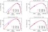 |
Fig. 1 Examples of SEDs and fits for four sources from our sample. Black diamonds with error bars are the IRIS 3THz and Planck 857, 545 and 353GHz flux densities, expressed in the νIν = constant colour convention. Two fits have been performed, one with β = 2 (blue) and the other with β free (red). For comparison with the data (black diamonds), the expected flux densities for the two fits with the same colour convention are represented with blue squares and red plus signs. The quality of each fit can be judged by comparing the estimated flux densities in each band (i.e., blue squares and red plus signs), with the actual measurements (i.e., black diamonds with error bars). Two envelopes are overlaid in the case of β free: the (T + σT, β − σβ) modified blackbody emission model (red dotted curve), and the (T − σT, β + σβ) model (red dashed curve). |
The cold sources extracted by the above procedure are distributed over the whole sky. Their flux densities at 857GHz varies by about 3 orders of magnitude, a broad range that primarily follows that of the source distances, although intrinsic variations in source luminosity may contribute. The S3000/S857 source colour also spans almost two orders of magnitude for most of the sources (Fig. 2).
We attempt in the following SED analysis to infer basic observational properties of these sources. Given the large variety of objects and environments represented in this catalogue, and the fact that the SEDs comprise only four bands (the IRIS 3THz and the three highest frequency Planck bands at 857, 545 and 353GHz), it has not been possible to carry out a complex modelling of the sources, taking into account dust population variations or radiative transfer (e.g., Compiègne et al. 2011; Bernard et al. 2008; Doty & Leung 1994; Juvela & Padoan 2003). Instead, we assume that the dust thermal emission at all frequencies is optically thin (this assumption is validated in Sect. 4.4), and that the SED can be approximated by a single modified blackbody emission law:  (4)where Sν is the flux density at the frequency ν integrated over the solid angle Ωc = πσMajσMin with σMaj and σMin the major and minor axis of the Gaussian ellipse of the source, Bν(T) is the Planck function at temperature T, NH2 is the column density, μ = 2.33 is the mean molecular weight, and mH is the mass of atomic hydrogen. The dust opacity κν is defined by
  (5)where κ0 is the value in cm2g-1 of the opacity at the reference frequency ν0, and β is the dust emissivity spectral index. This modelling involves a maximum of three free parameters (T, β and normalisation) to fit four data points, yielding at least one degree of freedom.
The fitting procedure is based on a reduced χ2 analysis, and uses the 1σ uncertainties on the input flux densities derived from the Monte Carlo analysis of Sect. 2.5, i.e., 40% in the IRIS 3THz band and 8% in Planck bands. The χ2 minimisation is performed on a pre-calculated grid taking into account the colour correction as defined in Planck HFI Core Team (2011b) and gives the exact minimum of χ2 in the (T, β, normalisation) space at the grid resolution, i.e., 0.01K in T and 0.01 in β. It also provides the associated 1σ uncertainty of the parameters by integrating the likelihood over the grid. We try two alternative models, which we now describe.
Firstly, we fix the spectral index to β = 2 (Boulanger et al. 1996). The χ2 minimisation is then performed on the T and normalisation parameters only, leading to two degrees of freedom. We provide a few examples of such SEDs and associated fits in Fig. 1, for various cases of temperature and spectral index, with more examples given in Appendix D. However, the colour–colour diagram of Fig. 2 shows that single modified blackbody emission models with β = 2 cannot explain the variety of cases present in the data. Furthermore, the quality of the SED fits in the case of β = 2 is illustrated in Fig. 3 which shows the distribution of the reduced χ2 as a function of temperature. In the case of fixed β = 2 (dark solid contours), the lower the temperature, the poorer the quality of the χ2 fit.
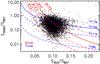 |
Fig. 2 Colour–colour diagram of the photometrically reliable catalogue: flux density ratio S3000/S857 versus S353/S857. The red lines show the domain of the single modified blackbody emission models with fixed values of β. The blue lines show the domain of the single modified blackbody emission models for fixed values of the temperature. The locus β = 2 (red solid line) appears to be insufficient to fit all the observational data points (black dots) of the C3PO photometrically reliable catalogue. |
Secondly, we perform a three parameter χ2 fit (on T, β and normalisation). This introduces an additional degeneracy in the fit results that is discussed below. The impact on the fit quality is illustrated in Fig. 3: in the case of β being free (red dashed contours), the distribution of the reduced χ2 varies less over the range of temperatures than when β is held fixed. The absolute value of χ2 is lower than in the case β = 2, as expected with the introduction of an additional free parameter to the fit. In the framework of a single modified blackbody emission modelling of the SEDs, assuming a free β results in a better fit to the observations although the best fit temperatures are nearly the same.
The known T − β degeneracy (e.g., Shetty et al. 2009b) could affect these determinations. Figure 4 shows the distribution of the fit parameters in relation to the colour ratios. For sources with S3000/S857 > 0.1, this ratio is a good tracer of the temperature. Of special interest in our survey are the sources dominated by intrinsically cold dust. For sources with S3000/S857 < 0.1, 99% of them show a temperature below 12K in the case of β free, and 96% of them below 13K in the case of β = 2, showing that the T–β degeneracy is not significantly affecting the fraction of cold sources in this sample. This is illustrated in the two left upper panels of Fig. 2. The lower left panel shows that they have a corresponding high dust emissivity spectral index β. Not surprisingly, the S353/S857 ratio is a tracer of β, but the fact that the correlation shows a large scatter is an indication that a fraction of the sources are cold enough not to be in the Rayleigh-Jeans domain in that frequency range. On the contrary, the temperature is not constrained by the S353/S857 ratio (right middle panel). The dependence on temperature seen for the β = 2 case (right upper panel) is an artifact imposed by the fixed value of β, leading to a bad fit thus not a good temperature determination. Figure 2 shows that for β = 2 (red solid line), a low S353/S857 ratio forces the solution to high temperatures, that may not be compatible with low S3000/S857 values (see two left panels of Fig. 4). For the cold sources selected with S3000/S857 < 0.1 and S353/S857 < 0.1 (narrow SEDs), representing ≈ 7% of the photometrically reliable sample, we are forced to keep β free in order to obtain reasonable fits; this is not the case for warm sources. If instead of fitting with a single temperature, we assumed a temperature distribution, then this would of course lead to even larger values of β.
We can see on the few SEDs shown in Fig. 1 that the IRIS point at 3THz plays a crucial role in modelling these SEDs, and obtaining the resulting temperature and spectral index estimates. Low estimates of the flux density at 3THz lead to low temperature estimates and high β values. For this reason special care has been taken to properly estimate the accuracy of the flux density measurements in all bands (and especially at 3THz) using Monte Carlo analysis (see Sect. 2.5). More details on the distribution of the temperature and β estimates are presented in Sects. 4.1 and 4.2.
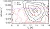 |
Fig.3 2D histogram of the reduced χ2 of the SED fitting as a function of the temperature Tc (see Sect. 4.1) for the photometrically reliable catalogue. The contours represent the 90%, 75%, 25%, 5% and 1% levels of the maximum of the 2D histogram over the (χ2, Tc) space. Case 1 (black solid line): reduced χ2 obtained for β = 2 as a function of the temperature inferred from the fit. When temperature becomes lower, more objects have a larger χ2. Case 2 (red dashed line): reduced χ2 as a function of the temperature obtained with a free β. The threshold χ2 = 2 (dash-dotted blue line) indicates the maximum level of χ2 that ensures a reasonable fit. |
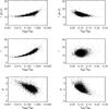 |
Fig.4 Dependence of the temperature of the cold clumps and the dust emissivity spectral index β on the colours at low and high frequency around 857GHz. The temperature is obtained by performing an SED fit with a fixed β = 2 (upper panels) and a variable β (middle panels), while the associated β is shown in the bottom panels. All quantities are given as a function of the S3000/S857 colour (left column) and of the S353/S857 colour (right column). |
Statistics of the Monte Carlo analysis performed to estimate the robustness of the photometry algorithm.
2.5. SED fitting quality assessment
To assess the accuracy of our photometry algorithm, we have performed Monte Carlo (MC) simulations. A total of 10000 simulated sources are randomly injected into the all-sky IRIS and Planck maps. The simulated SEDs are assumed to follow a modified blackbody form. The temperature T is randomly distributed between 6K and 20K, The associated spectral index β follows the Archeops distribution (Désert et al. 2008) β = (11.5 ± 3.8) × T − 0.66 ± 0.054. This gives values from β = 3.5 at 6K to β = 1.6 at 20K, to which we add an additional random variation of 20%. As we will see later in Sect. 4.2, both the functional form and the dispersion of the β values are similar to what is seen in Planck data and, therefore, provide an adequate starting point for the estimation of the uncertainties. The normalisation of the SEDs is constrained by the flux density at 857GHz, which is chosen to follow a logarithmic random distribution ranging from 10 to 500Jy, covering 97% of the observed distribution. An elliptical Gaussian profile is assumed, with a FWHM spanning from 4.5′ to 7′and an ellipticity ranging from 0 to 0.87. All simulated flux densities take into account the colour corrections. The complete process of photometry described in Sect. 2.3 is then applied on this set of simulated data, providing an estimate of all recovered quantities: flux densities; FWHM; and ellipticity. A distinction is made between the various cases associated with the photometry flags introduced in Sect. 2.3. Statistical bias and 1σ errors are derived and listed in Tables 1 and 2, for all-sky and |b| < 25°, respectively. A more detailed description of these results is provided in Appendix A and illustrated in Fig. A.1.
This Monte Carlo analysis confirms why sources with Aper forced set to “on” should be rejected from the physical study, since for these sources flux densities are systematically under-estimated by about 60%. For sources for which only an upper limit at 3THz has been provided by the algorithm (Upper 3THz set to “on”), the flux density at 3THz is over-estimated by a factor of two. The discrepancy can reach a factor of three in regions close to the Galactic plane. This illustrates the limitations on any physical conclusions that could be drawn from this population of sources. When a bad fit of the 3THz background map has been obtained (Bad Sfit 3THz flag set to “on”), the main error comes from the highly biased estimate of the FWHM (+31%), leading to an over-estimate of the flux densities in all bands. This could happen when a strong source is embedded in a faint background structure (e.g., at high latitude), introducing a degeneracy between the fit of the central elliptical Gaussian and the polynomial fit of the background surface at 3THz. Although the bias and 1σ values of flux densities are smaller than in the Normal case, due to the strong signal of these sources, we reject this population from the physical analysis, because they could introduce erroneous estimates of the physical properties based on a highly biased source extent.
If we focus now on the Normal case, when the photometry algorithm has performed well, we first observe a slight bias of all flux estimates that is only due to the photometry algorithm and the process of warm background subtraction. The flux density of the cold residual at 3THz is over-estimated by 1.4% over the whole sky, and even more (+11.5%) in the Galactic plane. However, the flux densities in the Planck bands are under-estimated by 2–5%. The associated 1σ errors are about 6–7% on all-sky and 8–9% in the Galactic plane in the Planck bands and about 40% in the 3THz band. The impact of such a biased estimate of the fluxes will be discussed together with the results on the SED fitting in Sect. 4.1. Finally the FWHM estimates are biased by less than 1% and have an accuracy of about ± 18%, while the ellipticity does not present evidence of any bias, with an accuracy of ± 9%.
The Monte Carlo simulations described here demonstrate the robustness of our photometry algorithm, and justify the rejection of entire categories of objects using the photometry flags. After rejecting all sources that present at least one of the flags Aper Forced, PS Neg or Bad Sfit 3THz, the remaining robust sample consists of 9465 objects, divided into two categories: 1840 objects have only an upper limit estimate of the flux at 3THz; and 7625 that have well defined photometry in IRIS and Planck bands. We will focus on this last category of 7625 sources for the rest of the analysis on clump physical properties. Moreover, based on this MC analysis, we will adopt the following estimate of the 1σ uncertainty on flux densities: 40% for IRIS 3THz; and 8% for Planck bands. This error is much larger than the intrinsic pixel noise and so instrumental errors are neglected.
We have used the same set of MC simulations to assess the quality of the SED fitting procedure described in Sect. 2.4 and the impact on the temperature and spectral index estimates. This analysis shows that the recovered temperature is slightly under-estimated (~2% in the Galactic plane), while the associated spectral index is over-estimated by about 7%. The statistical 1σ uncertainties are about 6% and 8% for T and β, respectively. This will be discussed in more detail in Sect. 4.1.
2.6. Cross-correlation with existing catalogues
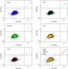 |
Fig.5 Colour–Colour diagram of the photometrically reliable catalogue (black dots). In each panel, the over-plotted symbols represent the positive cross-matches with non-ISM objects. The bottom right panel provides a summary of all positive cross-matches with non-ISM objects. |
As one step of the validation of the Planck detections, we have performed an astrometric search on the SIMBAD database3 for all known sources within a 5′ radius of the C3PO sources. There are a large number of such objects in the SIMBAD database, which raises the question of chance alignments. This is especially true for extragalactic objects, which have a reasonably isotropic sky distribution. To judge the number of chance alignments that can be expected by performing this kind of search, we have also conducted a SIMBAD cross-check on the positions of a set of 1000 MC simulated catalogues presented in Sect. 3.2.1. These MC realisations reproduce the object density of the Planck catalogue per bin of longitude and latitude. The results presented in Table 3 show that the number of coincidences in the ISM category (gathering the inter-stellar medium objects) is significantly greater in the C3PO catalogue than the chance alignments estimated from the MC simulations. On the contrary, the fraction of contaminants (i.e., Galaxies, QSOs, Radio Sources, Stars) is always lower in C3PO than in the MC realisations. Thus extragalactic objects and Galactic non-dusty objects are mostly rejected by the detection algorithm, whereas actual ISM structures are preferentially detected. A more detailed comparison between C3PO and the sub-category of the infra-red dark clouds (IRDCs) catalogues is presented in Sect. 5.
Nevertheless the association with probable contaminants in C3PO is still quite high (~10.5%, i.e., 1130 objects) and not all are necessarily the result of chance alignments. To disentangle chance alignment from real matches, we use colour–colour information, when reliable photometry is available (see Fig. 5). From the 7625 sources presenting robust photometry, 706 still have an association with probable contaminants. These objects are mostly distributed in the bottom-left corner of the diagram, typical of dust-dominated emitters. Only a few objects (17), located in the top right corner, show the colour–colour properties of radio emitters, suggesting real matches with extragalactic objects. Concerning the association with Stars, except for a few X-ray emitters, most SIMBAD matches seem associated with dusty emission, and so probably represent chance alignment. Thus the remaining sample of 689 probable contaminants, for which the probability of chance alignment is high, is not removed from the catalogue.
A total of 441 objects are rejected from the initial C3PO catalogue after this cross-correlation with ancillary data: 424 have no reliable photometry and are a priori rejected, due to a probable association with non-ISM objects; while the 17 others have reliable photometry but are clearly identified as extragalactic objects using the colour–colour information.
Cross-match with SIMBAD database for C3PO and simulated catalogues, for each category of SIMBAD type.
2.7. Building the catalogues
Starting from the 10783 source detections over the whole sky (see Sect. 2), two types of selection are applied. On the one hand, the cross-correlation with ancillary data identifies 441 suspicious candidates which may be associated with contaminants like extragalactic sources or stars (see Sect. 2.6). On the other hand, the quality of the flux density extraction has been quantified (see Sect. 2.3), providing flags that allow the rejection of entire categories of sources, because of their lack of robustness or biases in estimates for at least one of the four IRIS plus Planck bands. Four flags are used to discard the photometrically unreliable sources (see Sect. 2.5): Aper Forced (978); PSneg (229); Bad Sfit 3THz (140); and Upper 3THz (2356). We stress that overlap is possible between these flags. A total of 3158 objects have at least one of the flags listed above.
Using all this information, we build two catalogues: a complete catalogue and a photometrically reliable catalogue. The complete catalogue requires only the cross-check with ancillary data, leading to 10342 objects. The photometrically reliable catalogue requires both the cross-check with ancillary data, and the absence of a photometric flag, ensuring the robustness of the photometry. This last catalogue contains 7608 objects. Out of the 7608 sources, 40% have no counterpart in the SIMBAD database. In addition, these new detections have a similar SNR distribution as the complete catalogue (spanning from 4 to 30) and can be considered as reliable as those in the complete catalogue.
The Planck ECC sample has been defined as a subset of the C3PO catalogue, following two criteria: a signal-to-noise ratio greater than 15; and a temperature lower than 14K. This selection leads to 915 objects. Further details on the properties of this catalogue are given in Appendix C. The ECC has been included in the ERCSC (Planck Collaboration 2011c), as an auxiliary product. The ERCSC has been built frequency by frequency, and so some overlap exists with the ECC. A schematic description of these catalogues and the various sub-samples introduced in this work is given in Fig. 6.
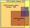 |
Fig.6 Partitioning of the two main C3PO samples: the complete (yellow) catalogue; and the photometrically reliable (orange) catalogue. The overlap between the sample for which we have distance estimates with those two catalogues is shown in brown. We finally overlay the ECC catalogue (blue) to show its overlap with the other samples. The proportional overlaps between samples are respected in this diagram. |
3. Spatial distribution
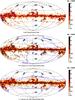 |
Fig. 7 Upper panel: all-sky map of the number of C3PO Planck cold clumps per sky area (2° × 2°). The ECC sources are overlaid as blue squares. Middle panel: contours of 12COJ = 1 → 0) line emission (0.1, 1, 4, 10, 30 Kkms-1) are over-plotted on the C3PO density map, which is set to zero where the CO map is not defined (limited by the blue contours). The resolution of the CO map is 2°. Lower panel: visual extinction contours (AV = 0.1, 0.5, 1, 2, 3, 4, 5, 6, 7 mag) are over-plotted on the C3PO density map, which is set to zero where AV is lower than 0.1 mag (blue contours). The AV map is also at a resolution of 2°. |
We now study the spatial distribution of C3PO clumps at three different scales, which we refer to as large, medium and small scales. The large scale study consists of an all-sky analysis of the correlation between cold clumps and Galactic morphology. The medium scale distribution handles shell- and loop-like Galactic objects, covering areas from a few deg2 up to 150deg2. Grouping properties are finally analysed at small scales, i.e., about the degree scale. Furthermore we provide an estimate of the heliocentric distance for a sub-sample of such sources.
3.1. All-sky association with Galactic morphology
The all-sky distribution of the 10342 sources of the complete C3PO catalogue is presented in the upper panel of Fig. 7. Mostly concentrated in the Galactic plane, the distribution clearly follows Galactic structures between latitudes of − 20° and + 20°. However, a few detections are observed at high Galactic latitude (|b| > 30°) and after cross-correlation with external catalogues have been confirmed not to be extragalactic in origin (see Sect. 2.6).
In the middle panel of Fig. 7, contours of the integrated intensity map of the COJ = 1 → 0 line are overlaid on the Planck cold clumps density all-sky map. This CO map is a combination of data from Dame et al. (2001) and NANTEN data (Fukui et al. 1999; Matsunaga et al. 2001; Mizuno & Fukui 2004), as defined in Planck Collaboration (2011d). The correlation between CO and C3PO cold clumps is quite impressive and demonstrates the robustness of the detection process and the consistency of the physical nature of these Planck cold objects. A detailed analysis shows that more than 95% of the clumps are associated with CO structures.
The lower panel of Fig. 7 shows the same kind of spatial correlation with the all-sky extinction, AV, map (Dobashi 2011). The AV map traces more diffuse regions of the Galaxy and extends to higher latitudes, where cold clumps are also present. About 75% of the C3PO objects are associated with an extinction greater than 1.
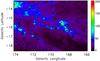 |
Fig. 8 Planck-HFI map at 857GHz (in MJysr-1) of the Taurus cloud area, showing the location and extent (at one FWHM) of the C3PO cold sources. C3PO cold sources are clearly distributed along the filaments of submillimetre dust emission, also known to be the coldest regions in IRAS colours (Abergel et al. 1994). |
3.2. Association with medium scale structures
Superimposed on the large-scale spiral structure of the Galaxy is a distribution of features known variously as shells, holes, loops, bubbles, arcs, filaments, superbubbles, supershells, etc., which has been referred to as the “Cosmic Bubble Bath” (Brand & Zealey 1975) or the “Violent ISM” (McCray & Snow 1979). These structures are characterised by an underdensity or overdensity of interstellar matter – either neutral or ionised – and are thought to be directly connected to the star-formation process (Blaauw 1991), forming loop-like, hole-like and filamentary-like structures. The Taurus cloud illustrates the case (see Fig. 8). This low-mass star-formation complex has been subject to extensive studies, due to its proximity (140pc, Elias 1978). The far-IR data show an intricate pattern of filaments, cavities and rings, which is also visible in the 12CO and 13CO data (Goldsmith et al. 2008). The C3PO cold clumps in this field are predominantly found along the filaments and shells.
Shells and loops are structures characterised by a deficiency of interstellar matter in their interior, accompanied by an over-density at the edges. They typically range in size from less than 100pc to more than 1000pc. Some, but not all, are observed to expand (for expanding Hi shells see e.g., Ehlerová & Palouš 2005). These types of objects can be well represented by elliptical rings. We provide here an overview of the distribution of the C3PO clumps with respect to the overall distribution of shells (as defined in Hi, see Heiles 1984) and loops (traced by far-IR data, see e.g., Schwartz 1987; Kiss et al. 2004). The cold clump surface density is remarkably high in the Taurus-Auriga-Perseus-Orion region (hereafter Taurus-Orion, see Fig. 9). Taurus-Orion is also characterised by a particular wealth of arcs, filaments and clustered sources, and we therefore use it as a special test case for our analysis, that we compare to the all-sky distribution. We stress that we have removed the region centred on the Galactic plane (|b| < 5°) from this analysis, due to the high confusion level.
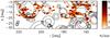 |
Fig. 9 Surface density map of the C3PO sources in the Taurus-Orion region, with the inner and outer boundaries of far-IR loops (Könyves et al. 2006) overlaid. |
In our discussion, we will refer to three selections: IN, the area inside the fitted profile of the loops/shells; ON, coincident with the ring itself; and OFF, the area outside all rings. We first carry out the all-sky correlation between the C3PO cold clumps and the different integrated areas relative to the shells/loops. We study this correlation shell-by-shell and loop-by-loop. For each shell/loop i we calculate the C3PO surface density  defined as the number of C3PO objects falling on the shell/loop divided by the area of the ring of the shell/loop.
Surface density (expressed in number per deg2) of C3PO sources and Monte Carlo simulations for Hi supershells in the three cases: IN shell; ON shell; and OFF areas.
3.2.1. Simulated samples
In order to evaluate the reliability of the observed distribution of C3PO objects, we produce MC simulated samples (hereafter MC samples). In each of the 1000 MC samples the observed number of sources (10342) are randomly placed onto the sky following the marginal distributions of the C3PO catalogue in (l,b) Galactic coordinates with a resolution of 5°.
To test the all-sky correlation we calculate the surface density values in each of the 1000 MC simulations for the different integrated areas (IN, ON, OFF). The mean values and standard deviations are presented in column “MC” of Tables 4 and 5. For the shell-by-shell and loop-by-loop analysis, the surface densities  are defined for each shell/loop i as the average over the 1000 MC realisations, with their associated standard deviation
  .
.
3.2.2. Hi shells
We investigate the spatial correlation of the C3PO cold clumps with the shells and supershells catalogued by Heiles (1984) using the 21-cm line surveys by Weaver & Williams (1973) and Heiles & Habing (1974). Heiles (1984) listed objects only at |b| < 10°, and physical sizes and distances are available for 34 Hi shells. The average diameter is 0.82kpc, at an average distance of 6.1kpc. We define a shell width individually for each Hi shell using the NASA LAMBDA4 Hi column density foreground maps.
The results of the all-sky analysis are compiled in Table 4. The distribution of the C3PO surface density ON the studied structures shows a significant excess compared to the simulations. The excess in the Taurus-Orion region compared to the MC samples ON the Hi shells is 2.6σ (respectively, 17σ for the all-sky case). On the contrary, the surface densities for OFF are slightly lower in the C3PO case compared to the simulated case. However, the surface density IN is not significantly different between C3PO and simulations. Thus C3PO cold clumps seem to be preferentially distributed ON the Hi shells, whether in the Taurus-Orion region or over the whole sky.
3.2.3. IRAS loops
IRAS loops were identified by Könyves et al. (2006) in the framework of an investigation of the large-scale structure of the diffuse ISM, started by Kiss et al. (2004) using the 60 and 100μm ISSA data (IRAS Sky Survey Atlas, Wheelock et al. 1994). Galactic infrared loops (GIRLs, Könyves et al. 2006) by definition must show an excess far-IR intensity confined to an arc-like feature extending to at least 60% of a complete ellipse-shaped ring. The thicknesses of the rings are given in the catalogue for all GIRLs. For about 20% of them a distance is also provided, that gives an average diameter of 0.09pc at an average distance of 1.1kpc. The potential role of the loops in the star-formation process has first been discussed by Kiss et al. (2006) and Tóth & Kiss (2007). The catalogue of IRAS GIRLs (Könyves et al. 2006) contains 462 far-IR loops, but for this analysis we only take into account the loops which are not completely within the Galactic plane (|b| < 5°), yielding 427 objects.
Figure 9 shows the surface density map of C3PO in the Taurus-Orion region with the far-IR loops overlaid. A first by-eye analysis already provides strong hints of a correlation between these loops and the distribution of the cold clumps. The statistical analysis in Taurus-Orion and all-sky (see Table 5) confirms these results, with, respectively, 11σ and 24σ excess of ON surface densities, compared to simulations. In the Taurus-Orion region the surface density ON the GIRLs is 6.3 times higher than the all-sky value. Moreover the all-sky surface density IN appears to be lower than the ON and OFF surface densities. This corresponds to the definition of the GIRLs, which says that the IN regions are “holes” in the interstellar medium.
When looking at the loop-per-loop analysis, over the total 427 GIRLS, 180 are not empty, and as many as 68 loops show a clear excess (>3σ) of C3PO surface densities ON the loops. These regions are interesting candidates to be followed-up, in order to study the correlation between the Planck cold clumps and those medium scale loops.
3.3. Small scale clustering of C3PO sources
3.3.1. Method
Groups in the C3PO sample were identified using the Minimal Spanning Tree (MST) method of Cartwright & Whitworth (2004), as described in Gutermuth et al. (2009) and Beerer et al. (2010). The MST is the unique network of straight lines joining a set of points, such that: i) the total length of all the lines (hereafter “edges”) in the network is minimised; and ii) there are no closed loops. The construction of such a tree is described by Gower & Ross (1969). Starting at any point, an edge is created joining that point to its nearest neighbour. The tree is then extended by always constructing the shortest link between one of its nodes and an unconnected point, until all the points have been connected (Cartwright & Whitworth 2004). Within the MST structure, groups can be separated as having “small” branch lengths between all members, i.e., less than some cutoff branch length.
We calculated the nearest neighbour distances for the C3PO clumps. Following Gutermuth et al. (2009) we computed the cumulative number of nearest neighbour distances with length d or smaller in the Taurus-Orion region, as a function of d. We derived the cutoff length as defined by the intersection between the two straight lines fitted on the two ends of the distribution. In our case, a cutoff length (i.e., maximum allowed distance between a group member core and a given subgraph) of 25′ was adopted. We note that the definition of groups strongly depends on the value used as the critical MST branch length; larger values tend to increase the number of group members, while smaller values tend to decrease the number of members (Kirk & Myers 2011).
3.3.2. Grouping properties
The results obtained with the MST method are compiled in Table 6. We first observe in the Taurus-Orion region that the average number of groups in the MC samples and in C3PO are similar. For the all-sky data, the MC samples show 30% fewer groups (at 25σ) than in C3PO. We also investigate the properties of sub-samples of larger groups, containing at least four objects. Thus we define the fraction of groups with at least four members compared to the number of all groups as NG4 + /NG. This fraction is 38% in the Taurus-Orion region and 28% over the whole-sky (see Table 6). These fractions are significantly higher than the mean values derived from the MC simulations. We see here the same behaviour for the Taurus-Orion region and for the whole sky. We also investigated the variation of NG and NG4 + /NG as a function of the cutoff length in the range 10′ to 30′ . For any cutoff length, the average NG and NG4 + /NG in the MC samples were 25–45% less than in the C3PO data. This analysis shows that the clustering of the C3PO cold clumps is real, and that larger groups are more common in C3PO than in random distributions.
Number and properties of identified groups in the C3PO data and the Monte Carlo simulations for the Taurus-Orion and for the all-sky distribution.
The elongation of groups was analyzed for all those having more than three members. Figure 10 shows a group of C3PO sources in the Taurus-Orion region. We used the Cartwright & Whitworth (2004) definition of cluster radius, Rc, as the distance between the mean position of all cluster members and the most distant sources. Following Schmeja & Klessen (2006) the area A of the cluster was estimated using the convex hull (the minimal convex set containing the set of points X in a real vector space V) of the data points. The convex hull radius, Rh, is defined as the radius of a circle with an area equal to the area A of the convex hull of the data points. Schmeja & Klessen (2006) describe the elongation measure ξ as: ξ = Rc/Rh.
For a fully spherical group, the elongation measure would be 1. If we approximate the shape of the groups with an ellipse, then elongation measures 1.4, 1.7, 2 and 3.2 correspond to axis ratios of 1:2, 1:3, 1:4 and 1:10, respectively. We calculated the elongation measure for all the 602 groups with N > 3. We found a mean elongation of ~2.2 in the Taurus-Orion region, and ~2.5 in the all-sky distribution (see Table 6). These elongations correspond to an axis ratio of 1:4.8 in the Taurus-Orion region and 1:6.3 in the all-sky sample. However, the mean elongation of the filaments in the MC samples (cf. Sect. 3.2.1) does not differ from that in C3PO in these regions (see Table 6). We also investigated the mean elongation in the C3PO data for different cutoff lengths, and we found that the average elongation of the groups is basically insensitive to this quantity. We actually do not see any evidence for elongation of the largest groups (N > 3) in the C3PO catalogue using this analysis.
3.4. Distance estimation
Distance estimates are essential to properly analyse the population of detected cold clumps. Four different methods are required to cover all the sources: association with IRDCs; association with known molecular complexes; a three dimensional extinction method using the Two Micron All Sky Survey (2MASS Skrutskie et al. 2006); and using Sloan Digital Sky Survey (SDSS, Abazajian et al. 2003) data.
3.4.1. Distances to IRDCs
Simon et al. (2006b) and Jackson et al. (2008) provide kinematic distance estimates for a total of 497 IRDCs extracted from the MSX catalogue (Simon et al. 2006a) that consists of 10931 objects. Kinematic distances are obtained via the observed radial velocity of gas tracers in the plane of the Galaxy. By assuming that the Galactic gas follows circular orbits and a Galactic rotation curve, an observed radial velocity at a given longitude corresponds to a unique Galactocentric radius. This means that in the inner Galaxy, two heliocentric distances are possible. This technique is only applicable in the plane and requires the availability of appropriate molecular data. We find 127 Planck cold sources, over the complete catalogue, associated with IRDCs that already have a kinematic distance estimate. This number decreases to 32 associations over the 7608 objects of the photometrically reliable C3PO catalogue.
A more recent study by Marshall et al. (2009) uses an extinction method, detailed in Sect. 3.4.3, on the same MSX catalogue of IRDCs, to derive the distance to 1259 objects. This yields 188 associations with C3PO clumps over the complete catalogue, and 47 over the photometrically reliable catalogue.
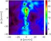 |
Fig.10 A sample group of C3PO sources in the Taurus-Orion region, overlaid on the cold residual map in MJysr-1. In this case, the elongation measure is ξ = 3.4. Black asterisks show the C3PO cold sources, solid lines indicate the MST edges and black dashed lines indicate the convex hull (defined in Sect. 3.3.2). The radius of the red dashed circle denotes Rc. Offset coordinates are used here, with the origin being the centre of the group. |
3.4.2. Distances to known molecular complexes
A simple inspection of the all-sky distribution of cold clumps suggests that it follows known molecular complexes. Many of these molecular complexes have distance estimates in the literature. To assign the distance of a complex to a particular cold clump we use the CO map of Dame et al. (2001) to trace the structure of the molecular cloud above a given threshold, and test for the presence of cold clumps inside this region. The association has been performed on 14 molecular complexes (see Table 7) located outside the Galactic plane, to reduce the level of confusion, leading to 1152 distance estimates over the complete catalogue and 947 on the photometric reliable catalogue.
3.4.3. Distances from extinction signature
Genetic forward modelling (using the pikaia code, Charbonneau 1995) is used along with the 2MASS data and the Besançon Galactic model (Robin et al. 2003) to deduce the three dimensional distribution of interstellar extinction towards the cold clump detections. The derived dust distribution can then be used to determine the distance of the sources, independently of kinematic models of the Milky Way. Along a line of sight that crosses a cold clump, the extinction is seen to rise sharply at the distance of the cloud. The method is fully explained in Marshall et al. (2006) and Marshall et al. (2009).
The distance, as determined by this technique, provides line of sight information on the dust distribution. However, it does not have sufficient angular resolution to perform morphological matches on the cold clumps. To ensure that the extinction rise detected along the line of sight is indeed related to the inner structure we perform a consistency check on the column density derived from the extinction and from the source flux density, corrected for its temperature. Only detections where the two column densities are in agreement within a factor of two are retained. This leads to distance estimates for 978 objects of the complete and photometrically reliable catalogue.
3.4.4. Distances from SDSS
Distances to cold clumps within 1kpc are obtained by analysis of distance-reddening relations for late spectral type stars within the line of sight to each source (Mc Gehee, in prep.). M stars are used because they can be dereddened to their true spectral types, while the stellar loci of the earlier spectral types is almost parallel to the reddening vector and hence the true spectral type cannot be recovered. We determine the intrinsic g − i colour from the measured Qgri = (g − r) − [E(g − r)/E(r − i)](r − i) reddening-invariant index using the median stellar locus of Covey et al. (2007). This is equivalent to dereddening to the M dwarf locus in the (g − r,r − i) colour–colour diagram. The reddening coefficients used are those of Schlafly et al. (2010) and photometric parallaxes are determined following Bochanski et al. (2010).
A simple profile model, consisting of a single step function convolved with a Gaussian (to model errors in the determination of distance modulus), is fit to the derived E(B − V) and distance values. Profiles with extreme fitted Gaussian widths, or with poor fits as judged by high rms values, are considered unreliable. Analysis of calibration fields containing the well-studied Orion B Cloud, reveal that the recovered distance moduli are underestimated by 0.35 mag, consistent with the bias expected from the Mdwarf multiplicity fraction.
This processing yields 1452 distance estimates in the entire catalogue, computed using stars within a 15′ radius of each position. Of these, 349 profiles, primarily in regions of lower extinction, are of acceptable quality.
3.4.5. Combined results
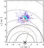 |
Fig. 11 Distribution of C3PO cold clumps as seen from the North Galactic Pole. Colours stand for methods used to estimate distance: molecular Complex association (green); SDSS extinction (light blue); 2MASS extinction (dark blue); IRDCs extinction (orange); and IRDCs kinematic (red). The red dashed circle shows the 1kpc radius around the Sun. Black dashed lines represent the spiral arms and local bar. The black circles give the limits of the molecular ring. |
The number of sources for which distances could be recovered depends on the method used (cf. Table 8). There is some overlap, but each method has its distinct advantages according to the distance range being considered.
The agreement between the estimates obtained with the SDSS extinction and the association to molecular complexes is good. While no bias is observed between these two distance estimates, the discrepancy can reach 50% in some cases, which gives an estimate of the uncertainty of those two methods. The agreement between the distance estimates obtained with the association to IRDCs and the 2MASS extinction is also fairly good, with about a 20% systematic over-estimate of the extinction method compared to the kinetic method, and with a maximum associated discrepancy of 50%. This study is in agreement with the comparison performed by Peretto & Fuller (2010) between the distance estimates of Marshall et al. (2009), Simon et al. (2006b) and Jackson et al. (2008) on IRDCs. On the other hand no agreement is obtained between the SDSS extinction and the 2MASS extinction methods on the fraction of objects (144) for which we have both estimates. The 2MASS distance estimates are about 2.5 times larger than the SDSS distance estimates on average, and can reach a factor of four in some cases. The 2MASS extinction method is not very sensitive to nearby extinction features (D < 1 kpc), as there are not enough stars to accurately determine the line of sight information. In contrast, the extinction method using SDSS is designed for nearby objects. For objects within 1kpc, we have preferably used SDSS distances when available, or molecular complex distances otherwise. We finally estimate that the uncertainty of our distance estimates is about a factor of two.
The number of objects for which we have a distance estimate is 2619, out of a total of 7608 objects in our photometrically reliable subset, i.e., ~34%. The distances of the cold clumps range from 0.1 to 7kpc, but they are mainly concentrated in the nearby Solar neighbourhood, as shown in Fig. 11. This type of distribution has already been demonstrated using simulations (see Fig. 10 of Montier et al. 2010). The lack of detections at large distances is mainly caused by the effects of confusion within the Galactic plane, which reduces the efficiency of the detection method. Nevertheless, when comparing the distance distribution of the C3PO cold clumps associated with MSX IRDCs with the total sample of Simon et al. (2006b) in Fig. 12, we notice that the fraction of C3PO-IRDC matches does not depend on distance and extends to 8kpc.
Because the subset of C3PO cold clumps with a distance estimate has been obtained using different methods, exploring various regions and distances over the sky, this sample appears heterogeneous. The completeness of the catalogue with respect to distances is quite difficult to assess. Thus we define two subsets for further analysis, for which we know that the sample is more reliable and homogeneous: the first subset (1790 objects) deals with local objects (D < 1kpc) and uses only estimates from molecular complex associations and SDSS extinction; the second subset (674 objects) focuses on more distant objects (D > 1kpc) and uses only 2MASS extinction estimates and IRDC associations.
Number of distance estimates available for the C3PO sources for each method.
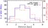 |
Fig. 12 Distance distribution of the MSX IRDCs (Simon et al. 2006b, solid blue line) and of the subset associated with the cold clumps of the complete C3PO catalogue (dash-dot-dot-dot red line) and the photometrically reliable subset of C3PO (dashed red line). |
4. Physical properties
4.1. Temperature
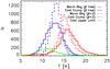 |
Fig. 13 Distribution of the temperature of the cold clumps (blue) of the photometrically reliable catalogue and their associated warm background (red) estimated inside the elliptical Gaussian of the clump itself, when using a fixed spectral index β = 2 (dashed line) or a variable β (solid line). The green curve gives the distribution of the temperature estimates for the C3PO sources that present only an upper limit at 3THz. This temperature is then only an upper limit estimate, associated with a lower limit on the spectral index β. |
The fitting procedure described in Sect. 2.4 has been applied to the SEDs including four bands (IRIS 3THz and Planck 857, 545 and 353GHz), to obtain temperature estimates. This process takes into account the 1σ uncertainties on the input flux densities derived from the Monte Carlo analysis in Sect. 2.5, i.e., 40% for the IRIS 3THz band and 8% for Planck bands. For each source, two temperatures are derived: (1) the temperature of the cold clump Tc, based on the SED fits of the cold residuals (Sect. 2.3); and (2) the temperature of the warm background Tw obtained from the SED fits performed on the warm background.
The resulting distributions of cold clump Tc and warm background Tw temperatures are shown on Fig. 13 for β = 2 (dashed lines) and for β free (solid lines). In the case where β is fixed at 2, the uncertainty on the temperature estimates is about 7%. The cold clump temperature Tc (blue dashed curve) distribution is shifted by a few degrees with respect to that of the warm background Tw (red dashed curve). This is consistent with what is expected from the extraction method of these cold sources. The temperatures of the cold clump and of the warm background peak at about 13K and 15K, respectively. The temperature distribution of the warm background extends over the known range in dust temperatures in the diffuse Galactic ISM. The temperature of the clumps Tc ranges from 9K to 16K, with a fraction 12% of them at Tc < 12K, as discussed in Sect. 2.4.
Treating β as a free parameter does not significantly affect these distributions. The associated spectral index β varies from 1.5 to 3, with an uncertainty of 21% and a mean value of 2.1 for cold clumps and 1.8 for the total emission, consistent with other studies based on Planck data (Planck Collaboration 2011d; Planck Collaboration 2011t; Planck Collaboration 2011g). The fraction of cold clumps with a temperature Tc < 12K is now 31%.
These results have to be corrected for two effects: the impact of the photometry algorithm itself; and the relative calibration uncertainty between IRIS and Planck. We first recall that a bias of about − 2% on T and 7% on β are induced by the photometry algorithm itself (see Sect. 2.5). On the other hand, the calibration uncertainty of flux densities (see Sect. B) does not introduced any bias on T or β, but generates an error of about 8% on β and from 3% to 5% on T, that should be added quadratically to the uncertainty due to statistical errors. All these considerations lead to a final range of temperature of the clump Tc spanning the range 7K to 19K, with an uncertainty of about 9%, and a spectral index β varying from 1.4 to 2.8, with an uncertainty of about 23%. The temperature of the clump Tc obtained in the case β free is defined as the reference temperature of the source, especially in the physical analysis. This temperature is indicative of the average temperature of these sources over the Planck beam.
In addition, 1805 sources from the complete catalogue present only an upper limit estimate for their flux densities at 3THz (without any other photometric flag), which constrains even better the dust temperature. The distribution of this upper limit temperature, shown as a green line in Fig. 13, peaks at 11K and varies from 7 K to 19 K. This Upper 3THz flag can be set when the confusion level is too high (in the Galactic plane), or when the sensitivity of IRAS (1Jy) is reached. This population of sources represents a very interesting sample of cold sources (another sub-sample of which is discussed in Sect. 5.2).
4.2. T–β relation
In order to examine the possible dependence between Tc and β, the values were fitted with a formula 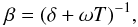 (6)(see Dupac et al. 2003). The least squares fit gave parameters δ = 0.020 and ω = 0.035. Figure 14 shows the distribution of the C3PO sources (black dots) in the β − T space, and the best fit line (blue solid curve), with its associated 1σ errors. This fit is in a good agreement with the relation derived from Archeops cold sources (Désert et al. 2008), which is overlaid in red solid lines, with its associated 1σ errors in red dashed lines. Because Planck and Archeops have submillimetre bands in common, it is encouraging to observe such an agreement between both populations of cold sources, even although the noise level on Planck detectors has been considerably reduced compared to the Archeops case, and the number of cold objects has been multiplied by about 30.
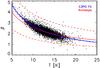 |
Fig. 14 The temperature and spectral index values from the catalogue and the fitted β(T) relations. The relation estimated from IRIS 3THz and the three highest frequency HFI channels is shown as a blue line with 1σ uncertainties denoted with dashed lines. The relation obtained from the Archeops survey (Désert et al. 2008) is shown as a red solid line, within ± 1σ red dashed curves. |
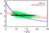 |
Fig. 15 Monte Carlo analysis of the noise effects on the β(Tc) relation. The black dots correspond to a synthetic sample, where the source flux densities have been scaled to be consistent with a constant value of β. The green points show the Tc and β values extracted from data, where we have added to these flux densities the estimated observational noise. The red line is the fit to these points. The observed relation obtained using C3PO sources (blue line, cf. Fig. 14) is significantly steeper. |
To estimate the uncertainties in the parameters, we carried out Monte Carlo simulations starting with the observed source flux densities. The uncertainties of the flux density values were taken to be 40% for the IRIS 3THz band and 8% for the three Planck bands. In each Monte Carlo realisation of the catalogue, we included additional variations in the calibration. The calibration factors were generated from a normal distribution and were taken to be 13.5% for the IRIS observations, 7% for the 545GHz and 857GHz data and 2% for the 353GHz Planck band. The same calibration scaling was applied to the two highest frequency Planck bands, because their calibration is based on correlation with the same FIRAS template (see Appendix B). With the estimated statistical uncertainties, the result for the analysis of the four bands is δ = 0.020 ± 0.001 and ω = 0.035 ± 0.001.
In the presence of observational errors, such as the uncertainties mentioned above, the T and β parameters become anticorrelated (Schwartz 1982; Dupac et al. 2003; Shetty et al. 2009b). We used MC simulations to determine the degree of anticorrelation that in our case can be produced solely by the observational noise. We started with the flux densities, temperatures, and spectral indices listed in the photometrically reliable C3PO catalogue. For each source, the flux densities were scaled with ν2.2 − β to produce a synthetic sample in which the spectral index is approximately constant but the deviations from the modified blackbody emission curve are consistent with the observations. The resulting (T, β) points are plotted in Fig. 15 as black dots. In the MC study, noise was added to the flux densities and the T and β values were estimated again. The observed relation is no longer flat (green points and the red least squares line) because of the correlated errors in the determination of the two parameters. The scatter is larger than for the observed points (Fig. 14), suggesting that the noise in this MC test was at least not underestimated. Nevertheless, the fitted β(T) curve is flatter than the relation observed in the catalogue (blue curve) and the hypothesis of an intrinsically flat β(T) relation can be excluded with more than 99% confidence. We recall here that for the coldest sources both the temperature and β are well constrained by the colours (see Sect. 2.4 and Fig. 4).
Moreover the process of integrating over the 5′Planck beam could mix components at various temperature. As studied by Shetty et al. (2009a) in the case of mixing two temperature components and by Malinen et al. (2011) in the case of a simple cold core modelling with internal heating source, the effect of temperature variations along the line-of-sight can produce such a Tc–β anti-correlation. Notice that the scatter of the MC test performed in this work (green points of Fig. 15) is compatible with the scatter obtained in Fig. 6 of Shetty et al. (2009a), given the uncertainties of Planck and IRIS data. However the observed spectral index β (>2) at low temperature (Tc < 12 K) cannot be reproduced by such temperature variations of individual components with β = 2.
Using PRONAOS data, Dupac et al. (2003) claimed to find an anti-correlation between the dust spectral index and temperature. Since then similar results have been obtained in studies on Archeops cold cores (Désert et al. 2008), Boomerang data (Veneziani et al. 2010) and recently Herschel data (Paradis et al. 2010). The temperature dependence of the spectral index we recovered is steeper than that found in PRONAOS data (Dupac et al. 2003). It is also slightly steeper than the relation reported for Archeops cores (see Fig. 15; Désert et al. 2008), although the Archeops relation is clearly compatible with our results given the uncertainties. Although a β(T) relation similar to that observed is expected for amorphous grains with disordered structure (Meny et al. 2007; Boudet et al. 2005) and for silicates, as shown more recently in laboratory experiments (Coupeaud et al. 2011), a robust physical interpretation cannot be inferred from our results because the clump sample is not a well-defined and homogeneous class of objects. Nevertheless, these studies suggest caution when interpreting Tc–β relations for samples containing star-forming clouds.
4.3. Extension and ellipticity
The extension and ellipticity of the sources, derived during step 1 of the photometry algorithm described in Sect. 2.3, have been compared with the local point spread function (PSF) provided by the FEBeCoP tool (Mitra et al. 2011) at 857GHz. This PSF takes into account the impact of projection on the sky of the optical beam of the instrument following the scanning strategy. Thus for each source, an elliptical Gaussian fit is applied on the PSF smoothed to 4.5′ to obtain the local FWHM θPSF, ellipticity ϵPSF and position angle ψPSF of the effective beam. The FWHM θ is defined as the geometric mean of the major and minor axis widths:  (7)and the ellipticity is given by
  (8)A few examples of FEBeCoP beams for Planck HFI detectors are given in Fig. B.5 of Paper II. Figure 16 compares the statistical distributions of the FWHM (upper panel), ellipticity (middle) and position angle (lower panel) between C3PO sources (solid line) and the local PSF at 857GHz (dashed line).
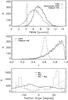 |
Fig. 16 Upper panel: distribution of the FWHM of the Planck detections compared to the distribution of the local PSF at 857GHz (dashed line). Middle panel: distribution of the ellipticity of the cold clumps (solid line) and of the local PSF (dashed line). Lower panel: distribution of the position angle of the elliptical Gaussian of the clumps (solid line), of the local PSF (dashed line), and the difference between them (dotted line). |
Cold clumps are clearly extended, with an average value of θc of 7.7′ compared to 4.3′ for the average PSF at 857GHz over the sky. Assuming that these compact sources are resolved by the Planck beam, we can deconvolve them to derive the inferred intrinsic source size θi (dot-dashed line in Fig. 16) using 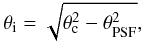 (9)where θc is the extent of the source and θPSF is the PSF extent. We find that θi/θPSF ≈ 1.4, and can conclude that we have resolved the sources. Nevertheless, as pointed out by Enoch et al. (2007) and Netterfield et al. (2009), the fact that the cold sources are mostly extended compared to the PSF may be an indicator of the hierarchical structure of these objects. Netterfield et al. (2009) show that the BLAST sources present the same behaviour, with a ratio between the inferred source size and the BLAST beam equal to 1.1. Enoch et al. (2007) obtained a value of 1.5 for cold cores in Serpens, Perseus and Ophiucus observed with Bolocam. Indeed these compact sources are associated with larger envelopes, presenting radial density profiles described by power laws with an exponent in the range − 2 to − 1 (Young et al. 2003).
Cold clumps are also mostly elongated, with a distribution of the ellipticity extending to values as large as 0.98 and peaking at around 0.9, compared to the mean value of 0.6 for the local PSF. Nevertheless, it has been shown that the time response of the instrument could also have an impact on the elongation of the sources along the scanning strategy. The importance of this effect is still difficult to assess, and could be relevant in some regions of the sky. Thus caution has to be used concerning this result. However, the C3PO cold clumps are not preferentially aligned with the major axis of the PSF; the position angles of the elliptical clumps and of the PSF are uncorrelated. As also stressed by Planck Collaboration (2011e), C3PO cold sources are often associated with filaments and parts of larger elongated cold structures where star formation occurs (see also Fig. 8). This was noted a long time ago by Barnard (1907) for Taurus, and it has more recently been investigated by Herschel observations in Polaris (Men’shchikov et al. 2010) and Aquila (Könyves et al. 2010).
When distances are available (see Sect. 3.4), we can derive the physical size of the sources, defined as the FWHM in units of pc. Figure 17 presents the distribution of the size obtained for 2619 sources. A distinction is made between local (D < 1kpc, dashed line) and distant (D > 1kpc, dot-dashed line) sources, as defined in Sect. 3.4.5. The distribution of size ranges from 0.2pc up to 20pc, and is highly heterogeneous. Since the distribution of the angular size is limited by the Planck resolution (i.e., ~5′) and the maximum size of these compact sources (i.e., ~12′), the associated physical size is totally driven by the distance estimate. With such a wide range of sizes, the nature of these cold sources can vary appreciably, from cold and very compact sources to large clouds of a few pc. This will be discussed in more detail in Sect. 5.
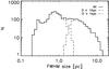 |
Fig. 17 Distribution of the physical size of the cold clumps in pc. The distinction is done between the local sample (D < 1 kpc, dashed line) and the distant sample (D > 1 kpc, dot-dashed line). |
4.4. Column densities
We compute the column density values  averaged over the clump solid angle following Eq. (4), and using the integrated flux density
  and temperature Tc of the cold clump. The main source of uncertainty here comes from the adopted value for κν. Large variations exist from one dust model to another, depending on the dust properties considered: composition (with or without ice mantles); structure (compact or fluffy aggregates); as well as size (see reviews from Beckwith et al. 1990; Henning et al. 1995). Dust models and observations show that κν values may vary by factors of 3–4 (or higher) from diffuse to dense and cold regions (Ossenkopf & Henning 1994; Kruegel & Siebenmorgen 1994; Stepnik et al. 2003; Juvela et al. 2010).
For this study, we have adopted the dust opacity from Beckwith et al. (1990), in agreement with the recommendation for dense clouds at intermediate densities, nH2 ≤ 105 (Preibisch et al. 1993; Henning et al. 1995; Motte et al. 1998), κν = 0.1(ν/1THz)β cm2g-1, where we take a standard emissivity spectral index β = 2. The computation is performed at ν = 857GHz, which is close to the 1THz of the formula, so that the impact of variation of the spectral index β remains small compared to the uncertainty in κν. For β varying from 1 to 3, the maximum variation of κν around the value obtained with β = 2 is 15%. The 857GHz band also provides the best SNR and the dust emission here is optically thin, with an average dust opacity at 857GHz of τ ~ 5 × 10⁻⁴ ≪ 1. We have checked that this is still the case at 3THz, with an average value of τ ~ 10-2. This validates the initial assumption on opacity adopted for this work.
For the clumps which have no distance estimate, we have also determined an approximate averaged volume density value with  (10)where the third size dimension of the object is taken as equal to the minimum value of the clump 2D size, σMin. The resulting number density ranges from 102 to 105cm-3, with a mean value of 2 × 103cm-3 (see Table 9).
The distribution of the column density as a function of the other physical parameters derived is shown in Fig. 21. The values cover a wide range, from 1020 up to 1023cm-2, and are centred around a few times 1021. In comparison with previous studies, the peak of this distribution is lower than the typical values of a few times 1022, inferred in cold cores observed from ground-based telescopes in nearby star-forming regions (Motte et al. 1998; Kauffmann et al. 2008; Enoch et al. 2008; Curtis & Richer 2010; Belloche et al. 2011). This can be explained by the Planck resolution, that preferentially selects quite extended objects, diluting sources smaller than the 5′ beam. Nevertheless, we observe a few objects with column density greater than 1023cm-2, even at the Planck resolution. These few objects could be precursors of massive stars, or high mass star-formation regions.
Finally, we observe that even the densest clumps (with high column densities) cannot reach temperature lower than 7K. This is in excellent agreement with recent observations of cold cores using Herschel (e.g., Wilcock et al. 2011; Peretto et al. 2010).
4.5. Mass distribution
We can define the mass integrated over the clump by  (11)where Sν is the integrated flux density at frequency ν = 857GHz, D is the distance, κν is the dust opacity (or mass absorption coefficient) as defined in Sect. 4.4, and Bν(T) is the Planck function for dust temperature at T. The uncertainty in the mass estimate can be quite high, due to the propagation of large errors on the dust opacity (that could reach 50%) and on the distance estimate (about 100%) elevated by the square. These mass estimates are therefore only accurate to within a factor of 4.
Figure 18 shows the distribution of the mass of the total sample (solid line) and of the two subsets, D < 1kpc (dashed line) and D > 1kpc (dot-dashed line), as defined in Sect. 3.4.5. The range of masses of the detected sources ranges from 0.4M⊙ up to 2.4 × 10⁵M⊙, with a median value of 88M⊙. It covers a broad variety of objects, from cores to giant molecular clouds, as will be discussed in Sect. 5. The theoretical sensitivity limit of Planck to low-mass cold cores is not reached. It would be about 0.03M⊙, for a cold source located at 100pc with a column density of 1020cm-2 (i.e., the lower limit of our sample, see Fig. 21) filling the Planck beam of 4.5′. The lower mass limit in the C3PO sample, i.e., 0.4M⊙, is considerably larger because it is affected by the confusion level and the extraction process from the warm background.
4.6. Luminosity
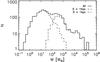 |
Fig. 18 Mass distribution for the total sample (solid line), nearby sub-sample (D < 1kpc, dashed line) and distant sub-sample (D > 1kpc, dot-dashed line). |
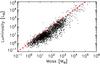 |
Fig. 19 Bolometric luminosity as a function of mass. The L = M limit is over-plotted as the red dashed line. |
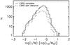 |
Fig. 20 Histogram of the L/M ratio for the total C3PO catalogue (solid line) and the sub-sample of 2619 objects for which a distance estimate has been obtained (dashed line). |
Bolometric luminosity is defined by 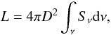 (12)where D is the distance, and Sν is the flux density for the clump. The bolometric luminosity, L, is integrated over the frequency range 300GHz < ν < 10THz, using the modelled SEDs derived from temperature and spectral index fitting (see Sect. 4.1). The L − M diagram is shown in Fig. 19. A large fraction of the objects is located below the L = M line (red dashed line) over the whole range of masses.
The quantity L/M has the advantage that it is independent of distance. Figure 20 shows the histogram of L/M for the photometrically reliable C3PO catalogue (solid line), and for the subset with distances (dashed line). The distributions of sources with and without distance estimates are very similar. This suggests that the methods used to estimate the distance do not introduce any strong distance-dependent selection bias in the sample compared to the complete catalogue. The lack of angular resolution prevents us from seeing internal sub-structures, so the presence of objects at various stages of evolution cannot be rejected, as also discussed in Roy et al. (2011) for the BLAST population in CygX. Nevertheless the L/M ratio provides an indication of the robustness of these sources as candidates for future star-forming regions, even at the Planck resolution. While 15% of the C3PO sources have a ratio L/M > 1L⊙/M⊙ and a temperature spanning from 13K to 19K, suggesting the presence of already evolved objects, the remaining 85% should include a fair number of early stage objects, and offer valuable candidates to be followed-up at higher resolution (see for example the studies performed with Herschel on Planck sources, Paper II, Juvela et al. 2010).
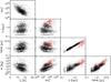 |
Fig. 21 Correlation matrix between various physical properties of the Planck C3PO sources, specifically temperature Tc, H2 column density |

Statistical description of the distribution of physical properties of the Planck C3PO catalogue of cold clumps.
5. Nature of the C3PO objects
5.1. A broad range of physical properties
As illustrated in Fig. 21 and summarised in Table 9, the C3PO catalogue contains cold sources covering a broad range of physical properties. This is due to the fact that these sources are detected as cold relatively to their environment, and that their distances cover more than an order of magnitude (note the D2 dependence of M in Fig. 21). It is therefore not surprising that most of the Planck cold sources, with sizes ranging from 0.2 pc to 18pc and masses from less than 1M⊙ to several times 105M⊙, are indeed a heterogeneous ensemble of objects. Only the smallest nearby Planck sources are likely to be cold cores according to the usual definition of being smaller than 0.2pc, with a density n > 104 cm-3 and mass M < 5M⊙ (cf. the categorization of Williams et al. 2000; Bergin & Tafalla 2007). Most of the others trace cold dust in large irregular structures up to the mass of giant molecular complexes (GMCs). In addition to the intrinsic dispersion of their properties, the background-foreground subtraction induces uncertainties which have been estimated by MC simulations (Appendix A.1). These show that the properties of the bulk of the sources are not significantly affected. Nevertheless it should be kept in mind that a small fraction of the sources (typically 1 to 3%) in the Galactic plane where the density of sources is of the order of 1deg-2, might be superpositions of nearby and distant sources affecting by large factors the derived physical parameters. One should thus treat with care the outliers in Fig. 21 (or Fig. 4) which might result from this effect. We note that a 4.5′ HFI beam leads to a resolution of 0.2pc in the nearest molecular complexes at 150pc. Thus identifying more distant cores requires higher angular resolution than the Planck beam.
In Juvela et al. (2010, 2011) and our companion Paper II, we have conducted a preliminary analysis using Herschel observations of a sample of ten cold clumps detected with Planck. These sources have been selected to sample different environments, from high latitude cirrus to nearby and remote molecular complexes. The high angular resolution of the Herschel SPIRE and PACS instruments has revealed rich and complex substructures. A range of properties have been observed: generally the substructures have been found to be denser and colder (down to 7K) than the Planck cold clump, except in two cases, where warmer sources have also been found in the Planck beam, in addition to cold dust.
The temperatures derived for the sources in the catalogue cover a range (7–19K) similar to previous estimates for a number a cold condensations detected using multi-wavelength submillimetre observations, for instance with the balloon-borne experiments: PRONAOS, T ~ 12K in star-forming and cirrus regions (Stepnik et al. 2003; Dupac et al. 2003; Bernard et al. 1999); Archeops, 7–18K (Désert et al. 2008); and BLAST, 9–14K (Netterfield et al. 2009). The highest temperatures found here (T > 15–19K) cannot realistically be called “cold clumps”, nevertheless they correspond to objects significantly colder than their observed environment. As a comparison, higher dust temperatures are obtained in the vicinity of Hii regions, even at Planck resolution, with typically T ~ 30K (Leto et al. 2009).
Most of the Planck clumps are not “compact point sources”, i.e., the result of the detection of small cores diluted within the large beam of Planck. On the contrary, they are found to be significantly extended and elongated. Independently of the angular resolution issue, it is difficult to distinguish here between the core, clump and cloud terminology introduced by Williams et al. (2000). The specific method used to identify and extract the core parameters should also to be considered (cf. for instance Curtis & Richer 2010). Our method is based on a colour signature of the objects, allowing the detection of the cold residual after the removal of the warm background. As discussed in Paper II, this may result in the identification of a different and more extended cold component than usually obtained with methods that identify structures on the basis of surface brightness (e.g., clumpfind, algorithms by Williams et al. 1994,or multi-scale wavelet analysis).
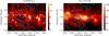 |
Fig. 22 GLIMPSE 8μm and Planck 857GHz maps (in MJysr-1) around the IRDC MSXDC G033.69 − 00.01 (green star). The contours show the cold residual map computed on the Planck 857GHz map and using the IRIS 3THz data. The positive contours (blue) are cold, while the negative contours (red) are warm. The C3PO cold clump is also shown as the dashed black ellipse. |
5.2. Comparison with IRDC catalogue
The plots of Fig. 21 suggest an overlap between the properties of the IRDCs and the most massive Planck clumps. Interestingly, the mass distribution of the dust cores within IRDCs, reaching up to 103M⊙, (Rathborne et al. 2010) suggests that the most massive Planck clumps, like IRDCs as a whole, are ensembles of cores arranged into larger structures similar to giant molecular complexes (GMCs).
Figure 22 provides an illustration of a common Planck and MSX detection in the case of MSXDC G033.69 − 00.01 (Simon et al. 2006a). The contours of the cold residual emission (in blue, light blue and red) are overplotted on the GLIMPSE 8μm intensity maps. The ellipse showing the Planck clump (dashed line) extracted from our detection method encompasses the absorption feature signature of the IRDC on the near-IR map. We note that the Planck size is larger than the extent of the MSX absorption. In the high-resolution map provided by GLIMPSE, substructures can be seen inside the extinction pattern.
This figure also illustrates the capability of the extraction method to isolate cold components in regions of bright emission containing a high level of confusion. In this field, it is striking to see how the brightest spots coincide with the warm component (traced in red), although the cold emission is mixed and hidden inside an extended warmer background emission. The object with an average column density of 6.5 × 1022cm-2, a mass of 2.4 × 10⁵M⊙ (at a distance of 7.1kpc) and a temperature of 12K, is among the most extreme in the distributions shown in Fig. 21. Eleven dense cores of mass ranging between 100 and 1300M⊙ have been detected in this IRDC at 1.2mm (Rathborne et al. 2006), and only three of them are associated with mid-IR emission. An IRAS source is also associated with one of these objects. This IRDC is therefore not among the youngest and coldest, that have not yet started to form stars. Nevertheless only a few cores are warm, contributing about 2 × 10³M⊙ of warm dust (Rathborne et al. 2006) out of the dust mass seen by Planck, or only 1% of the total dust mass.
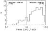 |
Fig. 23 Ratio of the angular extent of C3PO clumps and MSX IRDCs. |
A cross-match between C3PO sources and the MSX catalogue of 10931 IRDCs (Simon et al. 2006a) leads to 469 (136 in the photometrically reliable catalogue) Planck cold clumps associated with 1007 (296, respectively) MSX IRDCs. Less than 8% of the Planck clumps inside the region surveyed by MSX have no directly association with an IRDC. Indeed a comparison of the angular size of these objects is presented in Fig. 23, and shows that the C3PO objects are more extended than the IRDCs. Part of this effect is due to the very different spatial resolution of the MSX instrument at 8μm (28′′ versus 5′ with Planck). Most of the IRDCs appear as elongated irregular structures of length L and width L/a (a being the aspect ratio, a > 1); their size, defined as the geometric mean, is thus L/a0.5 (Simon et al. 2006a). With its large beam, Planck does not resolve the IRDCs in width, but does so in length for the largest ones. Therefore, for the largest IRDCs, we have the ratio of C3PO size to IRDC size being ~ a0.5 > 1, as seen in Fig. 22. The C3PO sizes, however, may be genuinely larger than those of IRDCs detected in absorption. In fact it appears that Planck is sensitive to dust column densities smaller than 1021cm-2 and colder than 15K (cf. Fig. 21), while MSX (and Spitzer IRAC) absorption measurements have a sensitivity threshold of 3 × 1021cm-2 (Peretto & Fuller 2010). Extended regions of cold dust with column densities between 3 × 1020cm-2 and 3 × 1021cm-2 are therefore detectable by Planck with no absorption counterparts at 8μm (as observed in Fig. 22).
We have also performed a cross-match with the Spitzer catalogue of IRDCs (Peretto & Fuller 2009), leading to 321 (78 in the photometrically reliable catalogue) Planck cold clumps associated with 1382 (356, respectively) Spitzer IRDCs. It is shown in Fig. 24 that the C3PO clumps could contain up to eight MSX IRDCs and 15 Spitzer IRDCs. Furthermore, the median distance between IRDCs in the MSX and Spitzer catalogues are 2.9′ and 1.7′, respectively, values which are lower than the C3PO typical extent that is about 6′; this supports the presence of multiple IRDCs inside the C3PO clumps. However, projection effects have to be taken into account when dealing with such Planck sources located in the Galactic plane, and caution has to be used when considering the number of associated IRDCs.
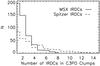 |
Fig. 24 Number of IRDCs found inside the Planck cold clumps when a match has been obtained with the MSX catalogue (Simon et al. 2006a) and the Spitzer catalogue (Peretto & Fuller 2009). |
6. Summary and perspectives
The three highest frequency channels of Planck, provide a census of cold dust sources in the Galaxy. To determine the properties of the coldest sources, they have to be extracted from the emission of their warmer background. This is done with a dedicated source extraction algorithm, CoCoCoDeT (Montier et al. 2010) that operates on the Planck maps combined with those at 3THz from the IRAS survey. The output, the Cold Clump Catalogue of Planck Objects (C3PO), is the first such all-sky catalogue of cold dust sources. We stress that this method does not provide a complete sample of cold sources in the Galaxy, due in a large part to confusion in the Galactic plane, and that it can only distinguish sources that are sufficiently colder than their background. The complete catalogue consists of 10342 objects, out of which the photometrically reliable catalogue comprises 7608 sources, for which physical characteristics such as flux densities, temperatures, angular extents, ellipticities and column densities are inferred from their SEDs. Among these a sub-sample comprises 2619 sources with distance estimates, for which physical sizes, masses, and average densities can also be estimated. In this paper we have performed a statistical analysis of these samples of cold objects and analysed their physical properties.
The temperature of the Planck cold sources ranges from 7K to 19K and its distribution peaks at about 13K. The great value of the C3PO catalogue is to provide a large number of very cold objects for follow-up studies, about 600 having a temperature Tc < 10K. Not only is this a large number compared to the already known cold sources in the Galaxy, but they are distributed over the whole sky, in the inner and outer Galaxy, and at high latitude, both near and far away from known star-forming regions. The diversity of the environments probed, from nearby diffuse molecular clouds to massive molecular complexes, and the possibility to map the mass distribution in such hierarchical environments opens new perspectives for understanding the evolution of molecular clouds towards star-formation activity in our Galaxy.
Another output of the SED fitting procedure is the dust emissivity spectral index β. We show that the data are not consistent with a constant value of β over the whole range of temperature, and that it is anticorrelated with the dust temperature. The anti-correlation observed for the coldest sources cannot be explained by a fitting degeneracy, given the narrow range of SEDs observed.
As expected, the Planck cold clump population is closely associated with Galactic structures, especially the molecular component, and is mainly distributed within the Galactic plane. Nevertheless, since the detection of cold sources inside the thin Galactic plane is difficult (due to the high confusion level), most of the detections are located within a few kpc of the Sun.
The mass of the cold sources for which the distance is known varies between 0.4M⊙ and 2.4 × 10⁵M⊙, and their size ranges from 0.2 to 18pc, with average density between 102cm-3 and 105 cm-3. This broad range of properties makes the C3PO catalogue a heterogeneous ensemble of cold objects in the Galaxy. While a few appear as actual cold protostellar core candidates, most of the C3PO sources appear rather to be larger structures, ranging from interstellar clouds up to giant molecular complexes for the most massive. A cross-match between C3PO sources and IRDCs from MSX and Spitzer shows that massive C3PO cold clumps contain up to 15 IRDCs, and that the C3PO sources are statistically more extended than IRDCs. The example of the massive IRDC MSXDC G033.69 − 00.01, detected in extinction by MSX and in emission by Planck (see Fig. 22 in Sect. 5.2), shows Planck’s sensitivity to emission in the outskirts, which are not detected in mid-IR absorption, and thus Planck complement these extinction surveys when confusion is not too large. Furthermore, there is a subset of cold, extended (several pc) and massive ( > 103M⊙) C3PO sources that may have been revealed for the first time by the Planck survey (see Fig. 22).
By studying the correlation between the cold clumps and large scale structures, such as the IRAS loops, we show that the cold clump population is preferably distributed on such large shells. Another interesting property of the C3PO sources is their distribution along known filaments within molecular clouds, and the associated degree of ellipticity of the sources.
In summary, because of the limited resolution (4.5′), the C3PO catalogue has assembled a large variety of objects in terms of physical properties, Galactic environment, and evolutionary stage, providing a wealth of new sources for follow-up and detailed investigations at higher angular resolution. With that perspective, the Herschel follow-up key programme “Galactic Cold Cores” is a unique tool to study the substructure and physics of selected C3PO sources at the same frequencies (selection being performed on either their intrinsic properties or on their environment). Such an analysis has already started (Juvela et al. 2010) on Herschel Science Demonstration Phase Data, and is continued in Planck Collaboration (2011e).
Finally, a high reliability sub-sample of this large C3PO catalogue has been delivered to the community: the Early Cold Core (ECC) sample. This is part of the ERCSC (Planck Collaboration 2011c) and provides a list of 915 objects over the whole sky, with similar statistics at high flux densities to the C3PO sample but with temperatures less than 14K. The ECC provides opportunities for ground-based or Herschel follow-up of cold clumps. Specialised catalogues focused on homogeneous classes of astrophysical objects will be published in subsequent papers. In these papers, a special effort will be made to improve the distance estimates, to increase the volume explored in the Galaxy, and to provide better estimates of the physical parameters.
Planck (http://www.esa.int/Planck) is a project of the European Space Agency (ESA) with instruments provided by two scientific consortia funded by ESA member states (in particular the lead countries France and Italy), with contributions from NASA (USA) and telescope reflectors provided by a collaboration between ESA and a scientific consortium led and funded by Denmark.
The ERCSC is available here: http://www.sciops.esa.int/index.php?project=planck&page=Planck_Legacy_Archive).
The ERCSC is available here: http://www.sciops.esa.int/index.php?project=planck&page=Planck_Legacy_Archive).
Acknowledgments
A description of the Planck Collaboration and a list of its members can be found at http://www.rssd.esa.int/index.php?project=PLANCK&page=Planck_Collaboration. We acknowledge the use of the Legacy Archive for Microwave Background Data Analysis (LAMBDA). Support for LAMBDA is provided by the NASA Office of Space Science. This research makes use of the SIMBAD database, operated at CDS, Strasbourg, France.
References
- Abazajian, K., Adelman-McCarthy, J. K., Agüeros, M. A., et al. 2003, AJ, 126, 2081 [Google Scholar]
- Abergel, A., Boulanger, F., Mizuno, A., & Fukui, Y. 1994, ApJ, 423, L59 [NASA ADS] [CrossRef] [Google Scholar]
- Aguirre, J. E., Ginsburg, A. G., Dunham, M. K., et al. 2011, ApJS, 192, 4 [NASA ADS] [CrossRef] [MathSciNet] [Google Scholar]
- André, P.,Men’shchikov, A., Bontemps, S., et al. 2010, A&A, 518, L102 [NASA ADS] [CrossRef] [EDP Sciences] [Google Scholar]
- Barnard, E. E. 1907, ApJ, 25, 218 [NASA ADS] [CrossRef] [Google Scholar]
- Beckwith, S. V. W., Sargent, A. I., Chini, R. S., & Guesten, R. 1990, AJ, 99, 924 [NASA ADS] [CrossRef] [Google Scholar]
- Beerer, I. M., Koenig, X. P., Hora, J. L., et al. 2010, ApJ, 720, 679 [NASA ADS] [CrossRef] [Google Scholar]
- Belloche, A., Schuller, F., Parise, B., et al. 2011, A&A, 527, A145 [NASA ADS] [CrossRef] [EDP Sciences] [Google Scholar]
- Bergin, E. A., & Tafalla, M. 2007, ARA&A, 45, 339 [NASA ADS] [CrossRef] [Google Scholar]
- Bernard, J. P., Abergel, A., Ristorcelli, I., et al. 1999, A&A, 347, 640 [NASA ADS] [Google Scholar]
- Bernard, J.-P., Reach, W. T., Paradis, D., et al. 2008, AJ, 136, 919 [NASA ADS] [CrossRef] [Google Scholar]
- Bersanelli, M., Mandolesi, N., Butler, R. C., et al. 2010, A&A, 520, A4 [NASA ADS] [CrossRef] [EDP Sciences] [Google Scholar]
- Blaauw, A. 1991, in The Physics of Star Formation and Early Stellar Evolution, ed. C. J. Lada, & N. D. Kylafis, NATO ASIC Proc., 342, 125 [Google Scholar]
- Bochanski, J. J., Hawley, S. L., Covey, K. R., et al. 2010, AJ, 139, 2679 [NASA ADS] [CrossRef] [Google Scholar]
- Bontemps, S., André, P., Könyves, V., et al. 2010, A&A, 518, L85 [NASA ADS] [CrossRef] [EDP Sciences] [Google Scholar]
- Boudet, N., Mutschke, H., Nayral, C., et al. 2005, ApJ, 633, 272 [NASA ADS] [CrossRef] [Google Scholar]
- Boulanger, F., Abergel, A., Bernard, J., et al. 1996, A&A, 312, 256 [NASA ADS] [Google Scholar]
- Brand, P. W. J. L., & Zealey, W. J. 1975, A&A, 38, 363 [NASA ADS] [Google Scholar]
- Cartwright, A., & Whitworth, A. P. 2004, MNRAS, 348, 589 [NASA ADS] [CrossRef] [Google Scholar]
- Chapin, E. L., Ade, P. A. R., Bock, J. J., et al. 2008, ApJ, 681, 428 [NASA ADS] [CrossRef] [Google Scholar]
- Charbonneau, P. 1995, ApJS, 101, 309 [NASA ADS] [CrossRef] [Google Scholar]
- Compiègne, M., Verstraete, L., Jones, A., et al. 2011, A&A, 525, A103 [NASA ADS] [CrossRef] [EDP Sciences] [Google Scholar]
- Coupeaud, A., Demyk, K., Mény, C., & Nayral, C. 2011, A&A, 535, A124 [NASA ADS] [CrossRef] [EDP Sciences] [Google Scholar]
- Covey, K. R., Ivezić, Ž., Schlegel, D., et al. 2007, AJ, 134, 2398 [NASA ADS] [CrossRef] [Google Scholar]
- Curtis, E. I., & Richer, J. S. 2010, MNRAS, 402, 603 [NASA ADS] [CrossRef] [Google Scholar]
- Dame, T., Hartmann, D., & Thaddeus, P. 2001, ApJ, 547, 792 [NASA ADS] [CrossRef] [Google Scholar]
- Désert, F., Macías-Pérez, J. F., Mayet, F., et al. 2008, A&A, 481, 411 [NASA ADS] [CrossRef] [EDP Sciences] [Google Scholar]
- Dobashi, K. 2011, PASJ, 63, 1 [NASA ADS] [CrossRef] [Google Scholar]
- Doty, S. D., & Leung, C. M. 1994, ApJ, 424, 729 [NASA ADS] [CrossRef] [Google Scholar]
- Dupac, X., Bernard, J., Boudet, N., et al. 2003, A&A, 404, L11 [NASA ADS] [CrossRef] [EDP Sciences] [Google Scholar]
- Egan, M. P., Shipman, R. F., Price, S. D., et al. 1998, ApJ, 494, L199 [NASA ADS] [CrossRef] [Google Scholar]
- Ehlerová, S., & Palouš, J. 2005, A&A, 437, 101 [NASA ADS] [CrossRef] [EDP Sciences] [Google Scholar]
- Elias, J. H. 1978, ApJ, 224, 857 [NASA ADS] [CrossRef] [Google Scholar]
- Enoch, M. L., Young, K. E., Glenn, J., et al. 2006, ApJ, 638, 293 [NASA ADS] [CrossRef] [Google Scholar]
- Enoch, M. L.,Glenn, J., Evans, II, N. J., et al. 2007, ApJ, 666, 982 [NASA ADS] [CrossRef] [Google Scholar]
- Enoch, M. L., Evans, II, N. J., Sargent, A. I., et al. 2008, ApJ, 684, 1240 [NASA ADS] [CrossRef] [Google Scholar]
- Falgarone, E., & Puget, J. L. 1985, A&A, 142, 157 [NASA ADS] [Google Scholar]
- Faúndez, S., Bronfman, L., Garay, G., et al. 2004, A&A, 426, 97 [NASA ADS] [CrossRef] [EDP Sciences] [Google Scholar]
- Fixsen, D. J., Cheng, E. S., Cottingham, D. A., et al. 1994, ApJ, 420, 457 [NASA ADS] [CrossRef] [Google Scholar]
- Fukui, Y., Mizuno, N., Yamaguchi, R., et al. 1999, PASJ, 51, 745 [NASA ADS] [CrossRef] [Google Scholar]
- Goldsmith, P. F., Heyer, M., Narayanan, G., et al. 2008, ApJ, 680, 428 [NASA ADS] [CrossRef] [Google Scholar]
- Górski, K. M., Hivon, E., Banday, A. J., et al. 2005, ApJ, 622, 759 [NASA ADS] [CrossRef] [Google Scholar]
- Gower, J. C., & Ross, G. J. S. 1969, Appl. Stat., 18, 54 [CrossRef] [Google Scholar]
- Griffin, M. J., Abergel, A., Abreu, A., et al. 2010, A&A, 518, L3 [Google Scholar]
- Gutermuth, R. A., Megeath, S. T., Myers, P. C., et al. 2009, ApJS, 184, 18 [NASA ADS] [CrossRef] [Google Scholar]
- Hatchell, J., Richer, J. S., Fuller, G. A., et al. 2005, A&A, 440, 151 [NASA ADS] [CrossRef] [EDP Sciences] [Google Scholar]
- Heiles, C. 1984, ApJS, 55, 585 [NASA ADS] [CrossRef] [Google Scholar]
- Heiles, C., & Habing, H. J. 1974, A&AS, 14, 1 [NASA ADS] [Google Scholar]
- Hennemann, M., Motte, F., Bontemps, S., et al. 2010, A&A, 518, L84 [NASA ADS] [CrossRef] [EDP Sciences] [Google Scholar]
- Henning, T., Michel, B., & Stognienko, R. 1995, Planet. Space Sci., 43, 1333 [NASA ADS] [CrossRef] [Google Scholar]
- Hill, T., Burton, M. G., Minier, V., et al. 2005, MNRAS, 363, 405 [NASA ADS] [CrossRef] [Google Scholar]
- Jackson, J., Finn, S., Rathborne, J., Chambers, E., & Simon, R. 2008, ApJ, 680, 349 [NASA ADS] [CrossRef] [Google Scholar]
- Juvela, M., & Padoan, P. 2003, A&A, 397, 201 [NASA ADS] [CrossRef] [EDP Sciences] [Google Scholar]
- Juvela, M., Ristorcelli, I., Montier, L. A., et al. 2010, A&A, 518, L93 [NASA ADS] [CrossRef] [EDP Sciences] [Google Scholar]
- Juvela, M., Ristorcelli, I., Pelkonen, V.-M., et al. 2011, A&A, 527, A111 [NASA ADS] [CrossRef] [EDP Sciences] [Google Scholar]
- Kauffmann, J.,Bertoldi, F.,Bourke, T. L., Evans, II, N. J., & Lee, C. W. 2008, A&A, 487, 993 [NASA ADS] [CrossRef] [EDP Sciences] [Google Scholar]
- Kirk, H., & Myers, P. C. 2011, ApJ, 727, 64 [NASA ADS] [CrossRef] [Google Scholar]
- Kiss, C., Moór, A., & Tóth, L. V. 2004, A&A, 418, 131 [NASA ADS] [CrossRef] [EDP Sciences] [Google Scholar]
- Kiss, Z. T., Tóth, L. V., Balázs, L. G., & Könyves, V. 2006, Publications of the Astronomy Deparment of the Eotvos Lorand University, 17, 173 [NASA ADS] [Google Scholar]
- Könyves, V.,André, P.,Men’shchikov, A., et al. 2010, A&A, 518, L106 [NASA ADS] [CrossRef] [EDP Sciences] [Google Scholar]
- Könyves, V., Kiss, C., Moor, A., Kiss, Z. T., & Toth, L. V. 2006, VizieR Online Data Catalog, 346, 31227 [NASA ADS] [Google Scholar]
- Kruegel, E., & Siebenmorgen, R. 1994, A&A, 288, 929 [NASA ADS] [Google Scholar]
- Lamarre, J., Puget, J., Ade, P. A. R., et al. 2010, A&A, 520, A9 [NASA ADS] [CrossRef] [EDP Sciences] [Google Scholar]
- Leahy, J. P.,Bersanelli, M., D’Arcangelo, O., et al. 2010, A&A, 520, A8 [NASA ADS] [CrossRef] [EDP Sciences] [Google Scholar]
- Leto, P., Umana, G., Trigilio, C., et al. 2009, A&A, 507, 1467 [NASA ADS] [CrossRef] [EDP Sciences] [Google Scholar]
- Lombardi, M., & Alves, J. 2001, A&A, 377, 1023 [NASA ADS] [CrossRef] [EDP Sciences] [Google Scholar]
- Malinen, J., Juvela, M., Collins, D. C., Lunttila, T., & Padoan, P. 2011, A&A, 530, A101 [NASA ADS] [CrossRef] [EDP Sciences] [Google Scholar]
- Mandolesi, N., Bersanelli, M., Butler, R. C., et al. 2010, A&A, 520, A3 [Google Scholar]
- Marshall, D. J., Robin, A. C., Reylé, C., Schultheis, M., & Picaud, S. 2006, A&A, 453, 635 [NASA ADS] [CrossRef] [EDP Sciences] [Google Scholar]
- Marshall, D. J., Joncas, G., & Jones, A. P. 2009, ApJ, 706, 727 [NASA ADS] [CrossRef] [Google Scholar]
- Matsunaga, K., Mizuno, N., Moriguchi, Y., et al. 2001, PASJ, 53, 1003 [NASA ADS] [Google Scholar]
- McCray, R., &Snow, Jr., T. P.1979, ARA&A, 17, 213 [NASA ADS] [CrossRef] [Google Scholar]
- Mennella, A., Butler, R. C., Curto, A., et al. 2011, A&A, 536, A3 [NASA ADS] [CrossRef] [EDP Sciences] [Google Scholar]
- Men’shchikov, A., André, P., Didelon, P., et al. 2010, A&A, 518, L103 [NASA ADS] [CrossRef] [EDP Sciences] [Google Scholar]
- Meny, C., Gromov, V., Boudet, N., et al. 2007, A&A, 468, 171 [Google Scholar]
- Mitra, S., Rocha, G., Górski, K. M., et al. 2011, ApJS, 193, 5 [NASA ADS] [CrossRef] [Google Scholar]
- Miville-Deschênes, M., & Lagache, G. 2005, ApJS, 157, 302 [NASA ADS] [CrossRef] [Google Scholar]
- Mizuno, A., & Fukui, Y. 2004, in Milky Way Surveys: The Structure and Evolution of our Galaxy, ed. D. Clemens, R. Shah, & T. Brainerd, ASP Conf. Ser., 317, 59 [Google Scholar]
- Molinari, S., Swinyard, B., Bally, J., et al. 2010, A&A, 518, L100 [NASA ADS] [CrossRef] [EDP Sciences] [Google Scholar]
- Montier, L. A., Pelkonen, V., Juvela, M., Ristorcelli, I., & Marshall, D. J. 2010, A&A, 522, A83 [NASA ADS] [CrossRef] [EDP Sciences] [Google Scholar]
- Motte, F., Andre, P., & Neri, R. 1998, A&A, 336, 150 [NASA ADS] [Google Scholar]
- Motte, F., Zavagno, A., Bontemps, S., et al. 2010, A&A, 518, L77 [NASA ADS] [CrossRef] [EDP Sciences] [Google Scholar]
- Netterfield, C. B., Ade, P. A. R., Bock, J. J., et al. 2009, ApJ, 707, 1824 [NASA ADS] [CrossRef] [Google Scholar]
- Neugebauer, G., Habing, H. J., van Duinen, R., et al. 1984, ApJ, 278, L1 [Google Scholar]
- Olmi, L., Ade, P. A. R., Anglés-Alcázar, D., et al. 2009, ApJ, 707, 1836 [NASA ADS] [CrossRef] [Google Scholar]
- Ossenkopf, V., & Henning, T. 1994, A&A, 291, 943 [NASA ADS] [Google Scholar]
- Paradis, D., Veneziani, M., Noriega-Crespo, A., et al. 2010, A&A, 520, L8 [NASA ADS] [CrossRef] [EDP Sciences] [Google Scholar]
- Pérault, M., Omont, A., Simon, G., et al. 1996, A&A, 315, L165 [Google Scholar]
- Peretto, N., & Fuller, G. A. 2009, A&A, 505, 405 [NASA ADS] [CrossRef] [EDP Sciences] [Google Scholar]
- Peretto, N., & Fuller, G. A. 2010, ApJ, 723, 555 [NASA ADS] [CrossRef] [Google Scholar]
- Peretto, N., Fuller, G. A., Plume, R., et al. 2010, A&A, 518, L98 [NASA ADS] [CrossRef] [EDP Sciences] [Google Scholar]
- Planck Collaboration 2011a, A&A, 536, A1 [NASA ADS] [CrossRef] [EDP Sciences] [Google Scholar]
- Planck Collaboration 2011b, A&A, 536, A2 [NASA ADS] [CrossRef] [EDP Sciences] [Google Scholar]
- Planck Collaboration 2011c, A&A, 536, A7 [NASA ADS] [CrossRef] [EDP Sciences] [Google Scholar]
- Planck Collaboration 2011d, A&A, 536, A8 [NASA ADS] [CrossRef] [EDP Sciences] [Google Scholar]
- Planck Collaboration 2011e, A&A, 536, A9 [NASA ADS] [CrossRef] [EDP Sciences] [Google Scholar]
- Planck Collaboration 2011f, A&A, 536, A10 [NASA ADS] [CrossRef] [EDP Sciences] [Google Scholar]
- Planck Collaboration 2011g, A&A, 536, A11 [NASA ADS] [CrossRef] [EDP Sciences] [Google Scholar]
- Planck Collaboration 2011h, A&A, 536, A12 [NASA ADS] [CrossRef] [EDP Sciences] [Google Scholar]
- Planck Collaboration 2011i, A&A, 536, A13 [NASA ADS] [CrossRef] [EDP Sciences] [Google Scholar]
- Planck Collaboration 2011j, A&A, 536, A14 [NASA ADS] [CrossRef] [EDP Sciences] [Google Scholar]
- Planck Collaboration 2011k, A&A, 536, A15 [NASA ADS] [CrossRef] [EDP Sciences] [Google Scholar]
- Planck Collaboration 2011l, A&A, 536, A16 [NASA ADS] [CrossRef] [EDP Sciences] [Google Scholar]
- Planck Collaboration 2011m, A&A, 536, A17 [NASA ADS] [CrossRef] [EDP Sciences] [Google Scholar]
- Planck Collaboration 2011n, A&A, 536, A18 [NASA ADS] [CrossRef] [EDP Sciences] [Google Scholar]
- Planck Collaboration 2011o, A&A, 536, A19 [NASA ADS] [CrossRef] [EDP Sciences] [Google Scholar]
- Planck Collaboration 2011p, A&A, 536, A20 [NASA ADS] [CrossRef] [EDP Sciences] [Google Scholar]
- Planck Collaboration 2011q, A&A, 536, A21 [NASA ADS] [CrossRef] [EDP Sciences] [Google Scholar]
- Planck Collaboration 2011r, A&A, 536, A22 [NASA ADS] [CrossRef] [EDP Sciences] [Google Scholar]
- Planck Collaboration 2011s, A&A, 536, A23 [NASA ADS] [CrossRef] [EDP Sciences] [Google Scholar]
- Planck Collaboration 2011t, A&A, 536, A24 [Google Scholar]
- Planck Collaboration 2011u, A&A, 536, A25 [NASA ADS] [CrossRef] [EDP Sciences] [Google Scholar]
- Planck Collaboration 2011v, The Explanatory Supplement to the Planck Early Release Compact Source Catalogue (ESA) [Google Scholar]
- Planck Collaboration 2011w, A&A, 536, A26 [NASA ADS] [CrossRef] [EDP Sciences] [Google Scholar]
- Planck HFI Core Team 2011a, A&A, 536, A4 [NASA ADS] [CrossRef] [EDP Sciences] [Google Scholar]
- Planck HFI Core Team 2011b, A&A, 536, A6 [NASA ADS] [CrossRef] [EDP Sciences] [Google Scholar]
- Poglitsch, A., Waelkens, C., Geis, N., et al. 2010, A&A, 518, L2 [NASA ADS] [CrossRef] [EDP Sciences] [Google Scholar]
- Preibisch, T., Ossenkopf, V., Yorke, H. W., & Henning, T. 1993, A&A, 279, 577 [NASA ADS] [Google Scholar]
- Rathborne, J. M., Jackson, J. M., & Simon, R. 2006, ApJ, 641, 389 [NASA ADS] [CrossRef] [Google Scholar]
- Rathborne, J. M., Jackson, J. M., Chambers, E. T., et al. 2010, ApJ, 715, 310 [NASA ADS] [CrossRef] [Google Scholar]
- Robin, A., Reylé, C., Derrière, S., & Picaud, S. 2003, A&A, 409, 523 [NASA ADS] [CrossRef] [EDP Sciences] [Google Scholar]
- Rosset, C., Tristram, M., Ponthieu, N., et al. 2010, A&A, 520, A13 [NASA ADS] [CrossRef] [EDP Sciences] [Google Scholar]
- Roy, A., Ade, P. A. R., Bock, J. J., et al. 2011, ApJ, 727, 114 [NASA ADS] [CrossRef] [Google Scholar]
- Schlafly, E. F., Finkbeiner, D. P., Schlegel, D. J., et al. 2010, ApJ, 725, 1175 [NASA ADS] [CrossRef] [Google Scholar]
- Schmeja, S., & Klessen, R. S. 2006, A&A, 449, 151 [NASA ADS] [CrossRef] [EDP Sciences] [Google Scholar]
- Schuller, F., Menten, K. M., Contreras, Y., et al. 2009, A&A, 504, 415 [NASA ADS] [CrossRef] [EDP Sciences] [Google Scholar]
- Schwartz, P. R. 1982, ApJ, 252, 589 [NASA ADS] [CrossRef] [Google Scholar]
- Schwartz, P. R. 1987, ApJ, 320, 258 [NASA ADS] [CrossRef] [Google Scholar]
- Shetty, R., Kauffmann, J., Schnee, S., & Goodman, A. A. 2009a, ApJ, 696, 676 [NASA ADS] [CrossRef] [Google Scholar]
- Shetty, R., Kauffmann, J., Schnee, S., Goodman, A. A., & Ercolano, B. 2009b, ApJ, 696, 2234 [NASA ADS] [CrossRef] [Google Scholar]
- Simon, R., Jackson, J. M., Rathborne, J. M., & Chambers, E. T. 2006a, ApJ, 639, 227 [NASA ADS] [CrossRef] [Google Scholar]
- Simon, R., Rathborne, J. M., Shah, R. Y., Jackson, J. M., & Chambers, E. T. 2006b, ApJ, 653, 1325 [NASA ADS] [CrossRef] [Google Scholar]
- Skrutskie, M., Cutri, R., Stiening, R., et al. 2006, AJ, 131, 1163 [NASA ADS] [CrossRef] [Google Scholar]
- Stepnik, B., Abergel, A., Bernard, J., et al. 2003, A&A, 398, 551 [NASA ADS] [CrossRef] [EDP Sciences] [Google Scholar]
- Tauber, J. A., Mandolesi, N., Puget, J., et al. 2010, A&A, 520, A1 [NASA ADS] [CrossRef] [EDP Sciences] [Google Scholar]
- Tóth, L. V., & Kiss, Z. T. 2007, in IAU Symp. 237, ed. B. G. Elmegreen, & J. Palous, 124 [Google Scholar]
- Veneziani, M., Ade, P. A. R., Bock, J. J., et al. 2010, ApJ, 713, 959 [NASA ADS] [CrossRef] [Google Scholar]
- Ward-Thompson, D., Kirk, J. M., André, P., et al. 2010, A&A, 518, L92 [NASA ADS] [CrossRef] [EDP Sciences] [Google Scholar]
- Weaver, H., & Williams, D. R. W. 1973, A&AS, 8, 1 [NASA ADS] [Google Scholar]
- Wheelock, S. L., Gautier, T. N., Chillemi, J., et al. 1994, NASA STI/Recon Technical Report N, 95, 22539 [NASA ADS] [Google Scholar]
- Wilcock, L. A., Kirk, J. M., Stamatellos, D., et al. 2011, A&A, 526, A159 [NASA ADS] [CrossRef] [EDP Sciences] [Google Scholar]
- Williams, J. P., de Geus, E. J., & Blitz, L. 1994, ApJ, 428, 693 [NASA ADS] [CrossRef] [Google Scholar]
- Williams, J. P., Blitz, L., & McKee, C. F. 2000, in Protostars and Planets IV, ed. V. Mannings, A. P. Boss, & S. S. Russell (University of Arizona Press), 97 [Google Scholar]
- Wright, E. L., Eisenhardt, P. R. M., Mainzer, A. K., et al. 2010, AJ, 140, 1868 [NASA ADS] [CrossRef] [Google Scholar]
- Young, C. H.,Shirley, Y. L., Evans, II, N. J., & Rawlings, J. M. C. 2003, ApJS, 145, 111 [NASA ADS] [CrossRef] [Google Scholar]
- Zacchei, A., Maino, D., Baccigalupi, C., et al. 2011, A&A, 536, A5 [NASA ADS] [CrossRef] [EDP Sciences] [Google Scholar]
Appendix A: Monte Carlo quality assessment of the photometry
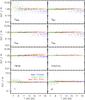 |
Fig. A.1 Comparison of the extracted and injected values of the Monte Carlo simulations performed to assess the quality of the photometry algorithm. Black dots refer to the nominal case, when red, blue and green dots stand for various flags of the photometry algorithm: Bad Sfit 3THz (red); Aper Forced (blue); and Upper 3THz (green). |
As presented in Sect. 2.5, we have performed a Monte Carlo analysis to assess the robustness of the photometry algorithm described in Sect. 2.3. A set of 10000 sources have been injected into Planck all-sky maps following a distribution of temperatures, dust spectral indices and flux densities in agreement with the observations. Figure A.1 compiles the relative errors between output and input quantities (flux densities, FWHM, ellipticity, temperature and spectral index) for the complete set of simulated sources as a function of the flags raised during the photometry estimate. Three flags have been investigated here: Aper Forced (blue); Bad Sfit 3THz (red); and Upper 3THz (green).
Appendix B: Impact of calibration uncertainty
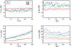 |
Fig. B.1 Bias and 1σ discrepancy of the temperature T and dust spectral index β estimates derived from a Monte Carlo analysis dedicated to studying the impact of the calibration uncertainties. Three cases have been studied: calibration uncertainty only (red lines); independent flux density errors (green); and calibration plus independent flux density errors (blue). |
The relative calibration uncertainty is known to be 13.5% for the IRIS 3THz data (Miville-Deschênes & Lagache 2005), and about 7% for the Planck high frequency bands at 857GHz and 545GHz, and 2% at 353GHz (Planck HFI Core Team 2011a). Here we investigate the impact of this error on temperature and spectral index estimates, considering that the uncertainty is not independent between all bands. The principle is to fix the two top Planck bands (545 and 857GHz) to follow the same relative calibration error, while the 3THz and the 353GHz bands remain independent. For a given temperature T and a dust spectral index β, SEDs are simulated using a modified blackbody model, including colour corrections. A 13.5% relative level of Gaussian noise is added on the 3THz flux densities, then another 7% noise realisation is added at 545GHz and 857GHz simultaneously, and a 2% noise realisation is added to the 353GHz flux densities. We also study the combination of a calibration error plus an independent error band per band, set to 20% and 10% for the 3THz and Planck bands, respectively. A third set of data is defined as our reference case and does not include any calibration error, but only an independent error per band. The T,β fitting algorithm described in Sect. 4.1 is applied on these three sets of SEDs, leading to an estimate of the bias and 1σ uncertainty of the output distribution, for T ranging from 6K to 25K and β spanning from 1.75 to 2.5.
The results are shown in Fig. B.1. The impact of the calibration uncertainty (in red) is very low compared to the size of the measurement error only (in green). In all cases, the bias on temperature and β is negligible or significantly lower than 1%. In both cases the bias level remains independent of T and β. On the other hand the 1σ uncertainty on the temperature goes from 3% to 8% at, respectively, 6K and 25K, due to calibration uncertainty only, and remains independent of β. The 1σ discrepancy on β is about 7–10% over this temperature range and it decreases of 3% when β goes from 1.75 to 2.5. This error is larger and much more sensitive to β in the case of measurement uncertainty (green curves). Thus the impact of the calibration uncertainty seems very small compared to the impact of the measurement error coming from the flux densities. Moreover, in the case of a combination of calibration and measurement uncertainties (in blue), both resulting uncertainties on T and β are found to add quadratically.
For this work, we consider separately the impact of the calibration uncertainty, and simply add the quadratic errors at the end of the processing. The values of the calibration uncertainties for T and β are provided in Tables B.1 and B.2 for a given set of T,β parameters.
Bias and 1σ error on the temperature due to the calibration uncertainty on flux densities in the IRIS 3THz and Planck 857, 545 and 353GHz bands, shown for a range of (T,β).
Bias and 1σ error on the spectral index β due to the calibration uncertainty on flux densities in the IRIS 3THz and Planck 857, 545 and 353GHz bands, shown for a range of (T,β).
Appendix C: The early cold core sub-sample
C.1. Selection criteria
The Early Release Compact Source Catalogue5 (ERCSC; Planck Collaboration 2011c) was released in January 2011. It includes the main ERCSC, where the point sources are detected in each separate channel map, but it also incorporates two specialised catalogues, the early Sunyaev-Zeldovich (ESZ) and the early cold cores (ECC). The ECC is a sub-sample of the full C3PO catalogue, obtained by applying the following two criteria:
-
1.
SNR > 15;
-
2.
TECC < 14K.
Here SNR is the signal-to-noise ratio of the detection, and TECC is the temperature derived from aperture photometry. However, in the case of the ECC, this temperature is derived in a different manner than described here for the C3PO. In the ECC, the photometry is carried out on the original Planck maps (i.e., maps that still retain the warm component of the diffuse dust emission), by placing an aperture of 5′ radius on top of the detection. The background is estimated using an annulus around the aperture with an inner radius of 5′ and an outer radius of 10′. Temperatures are derived from a fit to all four bands (IRIS 3THz and Planck 857, 545 and 353GHz) used to obtain the detection. While the annulus is efficient in subtracting the diffuse warm background, this estimate of the temperature does not take into account the real shape of the sources nor the subtraction of any warm envelope linked to the clump. It does, however, provide a straightforward estimate of the temperature that is provided in the ECC.
The signal-to-noise cut at SNR = 15 was selected based on the Monte Carlo Quality Assessment (MCQA) results performed in the framework of the ERCSC. Three sets of 1000 sources were injected into the IRIS and Planck maps. These sources were defined by temperature, spectral index and flux density at 857GHz, and their associated SEDs followed a modified blackbody model. Detection and photometry processing were then applied in these three sets of simulated maps, to find the proportion of detected sources and their recoveredflux densities. A reliability of 90% was required, where reliability is here defined as the fraction of detected test sources with less than 30% error in recovered flux density. The MCQA analysis showed that the choice of SNR = 15 ensured a reliability of 90% over the temperature range TECC < 14K in all three Planck bands (cf. Fig. 23 of Planck Collaboration 2011v). Hence, the ECC is 90% reliable, where the reliability is based on flux density, not detection.
C.2. Summary of the ECC
The above criteria lead to a sub-sample of 915 objects over the sky. Of these objects, 118 have no SIMBAD entry and are new detections. Thus at least 13% are new sources.
Simply due to the selection criteria, the ECC is the high-SNR and the cold tail of the C3PO distribution. The spatial distribution of the ECC objects is biased towards nearby, star-formation regions (e.g., Perseus, Taurus and Orion) where the SNR is high, while the Galactic disk is under-represented (see upper panel of Fig. 7). This is because of the higher confusion in the plane, so that the SNR tends to be lower there, but also because the dust temperatures in the plane tend to be higher. Not surprisingly, the derived column densities for the ECC objects are also biased towards the higher column densities in the C3PO distribution.
While the ECC does not contain this information, we have recovered distance estimates for some of the ECC objects, using the methods described in Sect. 3.4. Combining the distance information with the flux densities of the dust emission, we can estimate the mass of the sources. We find that the ECC objects are as varied in mass as the C3PO objects, ranging from what might be single cores (with a mass of a few M⊙, to clumps of tens and hundreds of M⊙, and even larger complexes of thousands of M⊙. Most of the objects for which we have mass estimates are in the range from 100 to 1000M⊙. The spatial resolution of Planck does not allow for a detailed morphological study of these sources, so the users of the ECC need to be aware that they are not looking at single cores in most of the cases; only high-resolution follow-up studies will reveal the exact morphology of these clumps.
The ECC is an excellent resource for follow-up studies. Highly reliable, it contains coordinates, aperture photometry, and the derived temperature and spectral index for each object, which observers can use to estimate their own fluxes, or molecular lines brightnesses to look for. The simple aperture photometry procedure used the derive the flux densities makes it easy to combine the ECC information with follow-up observations to obtain composite SEDs.
Appendix D: Examples of SEDs
We provide here a few examples of SEDs of C3PO sources which indicate temperatures: lower than 8K (Fig. D.1); between 8K and 10 K (Fig. D.2); and between 10K and 14K (Fig. D.3). SED fits are plotted for both fixed β = 2 and β being free.
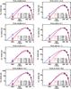 |
Fig. D.1 SEDs of selected C3PO sources with temperatures Tc < 8K. Black diamonds with error bars are the IRIS 3THz and Planck 857, 545 and 353GHz data. Two fits have been performed: one with β = 2 (blue); and the other with β free (red). For comparison with the data (black diamonds), the expected flux densities for the two fits, with the same colour convention, are shown with blue squares and red plus signs. The quality of each fit can be judged by comparing the estimated flux densities in each band, i.e., blue squares and red plus signs, with the actual measurements, i.e., black diamonds with error bars. Two models are overlaid to define an approximate error envelope in the case of β free: the (T + σT, β − σβ) modified blackbody emission model, in the red dotted curve; and the (T − σT, β + σβ) model in the red dashed curve. |
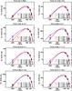 |
Fig. D.2 SEDs of selected C3PO sources with temperatures in the range 8–10K. See Fig. D.1 for details. |
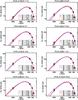 |
Fig. D.3 SEDs of selected C3PO sources with temperatures in the range 10–14K. See Fig. D.1 for details. |
All Tables
Statistics of the Monte Carlo analysis performed to estimate the robustness of the photometry algorithm.
Cross-match with SIMBAD database for C3PO and simulated catalogues, for each category of SIMBAD type.
Surface density (expressed in number per deg2) of C3PO sources and Monte Carlo simulations for Hi supershells in the three cases: IN shell; ON shell; and OFF areas.
Number and properties of identified groups in the C3PO data and the Monte Carlo simulations for the Taurus-Orion and for the all-sky distribution.
Statistical description of the distribution of physical properties of the Planck C3PO catalogue of cold clumps.
Bias and 1σ error on the temperature due to the calibration uncertainty on flux densities in the IRIS 3THz and Planck 857, 545 and 353GHz bands, shown for a range of (T,β).
Bias and 1σ error on the spectral index β due to the calibration uncertainty on flux densities in the IRIS 3THz and Planck 857, 545 and 353GHz bands, shown for a range of (T,β).
All Figures
|
Fig. 1 Examples of SEDs and fits for four sources from our sample. Black diamonds with error bars are the IRIS 3THz and Planck 857, 545 and 353GHz flux densities, expressed in the νIν = constant colour convention. Two fits have been performed, one with β = 2 (blue) and the other with β free (red). For comparison with the data (black diamonds), the expected flux densities for the two fits with the same colour convention are represented with blue squares and red plus signs. The quality of each fit can be judged by comparing the estimated flux densities in each band (i.e., blue squares and red plus signs), with the actual measurements (i.e., black diamonds with error bars). Two envelopes are overlaid in the case of β free: the (T + σT, β − σβ) modified blackbody emission model (red dotted curve), and the (T − σT, β + σβ) model (red dashed curve). |
| In the text | |
|
Fig. 2 Colour–colour diagram of the photometrically reliable catalogue: flux density ratio S3000/S857 versus S353/S857. The red lines show the domain of the single modified blackbody emission models with fixed values of β. The blue lines show the domain of the single modified blackbody emission models for fixed values of the temperature. The locus β = 2 (red solid line) appears to be insufficient to fit all the observational data points (black dots) of the C3PO photometrically reliable catalogue. |
| In the text | |
|
Fig.3 2D histogram of the reduced χ2 of the SED fitting as a function of the temperature Tc (see Sect. 4.1) for the photometrically reliable catalogue. The contours represent the 90%, 75%, 25%, 5% and 1% levels of the maximum of the 2D histogram over the (χ2, Tc) space. Case 1 (black solid line): reduced χ2 obtained for β = 2 as a function of the temperature inferred from the fit. When temperature becomes lower, more objects have a larger χ2. Case 2 (red dashed line): reduced χ2 as a function of the temperature obtained with a free β. The threshold χ2 = 2 (dash-dotted blue line) indicates the maximum level of χ2 that ensures a reasonable fit. |
| In the text | |
|
Fig.4 Dependence of the temperature of the cold clumps and the dust emissivity spectral index β on the colours at low and high frequency around 857GHz. The temperature is obtained by performing an SED fit with a fixed β = 2 (upper panels) and a variable β (middle panels), while the associated β is shown in the bottom panels. All quantities are given as a function of the S3000/S857 colour (left column) and of the S353/S857 colour (right column). |
| In the text | |
|
Fig.5 Colour–Colour diagram of the photometrically reliable catalogue (black dots). In each panel, the over-plotted symbols represent the positive cross-matches with non-ISM objects. The bottom right panel provides a summary of all positive cross-matches with non-ISM objects. |
| In the text | |
|
Fig.6 Partitioning of the two main C3PO samples: the complete (yellow) catalogue; and the photometrically reliable (orange) catalogue. The overlap between the sample for which we have distance estimates with those two catalogues is shown in brown. We finally overlay the ECC catalogue (blue) to show its overlap with the other samples. The proportional overlaps between samples are respected in this diagram. |
| In the text | |
|
Fig. 7 Upper panel: all-sky map of the number of C3PO Planck cold clumps per sky area (2° × 2°). The ECC sources are overlaid as blue squares. Middle panel: contours of 12COJ = 1 → 0) line emission (0.1, 1, 4, 10, 30 Kkms-1) are over-plotted on the C3PO density map, which is set to zero where the CO map is not defined (limited by the blue contours). The resolution of the CO map is 2°. Lower panel: visual extinction contours (AV = 0.1, 0.5, 1, 2, 3, 4, 5, 6, 7 mag) are over-plotted on the C3PO density map, which is set to zero where AV is lower than 0.1 mag (blue contours). The AV map is also at a resolution of 2°. |
| In the text | |
|
Fig. 8 Planck-HFI map at 857GHz (in MJysr-1) of the Taurus cloud area, showing the location and extent (at one FWHM) of the C3PO cold sources. C3PO cold sources are clearly distributed along the filaments of submillimetre dust emission, also known to be the coldest regions in IRAS colours (Abergel et al. 1994). |
| In the text | |
|
Fig. 9 Surface density map of the C3PO sources in the Taurus-Orion region, with the inner and outer boundaries of far-IR loops (Könyves et al. 2006) overlaid. |
| In the text | |
|
Fig.10 A sample group of C3PO sources in the Taurus-Orion region, overlaid on the cold residual map in MJysr-1. In this case, the elongation measure is ξ = 3.4. Black asterisks show the C3PO cold sources, solid lines indicate the MST edges and black dashed lines indicate the convex hull (defined in Sect. 3.3.2). The radius of the red dashed circle denotes Rc. Offset coordinates are used here, with the origin being the centre of the group. |
| In the text | |
|
Fig. 11 Distribution of C3PO cold clumps as seen from the North Galactic Pole. Colours stand for methods used to estimate distance: molecular Complex association (green); SDSS extinction (light blue); 2MASS extinction (dark blue); IRDCs extinction (orange); and IRDCs kinematic (red). The red dashed circle shows the 1kpc radius around the Sun. Black dashed lines represent the spiral arms and local bar. The black circles give the limits of the molecular ring. |
| In the text | |
|
Fig. 12 Distance distribution of the MSX IRDCs (Simon et al. 2006b, solid blue line) and of the subset associated with the cold clumps of the complete C3PO catalogue (dash-dot-dot-dot red line) and the photometrically reliable subset of C3PO (dashed red line). |
| In the text | |
|
Fig. 13 Distribution of the temperature of the cold clumps (blue) of the photometrically reliable catalogue and their associated warm background (red) estimated inside the elliptical Gaussian of the clump itself, when using a fixed spectral index β = 2 (dashed line) or a variable β (solid line). The green curve gives the distribution of the temperature estimates for the C3PO sources that present only an upper limit at 3THz. This temperature is then only an upper limit estimate, associated with a lower limit on the spectral index β. |
| In the text | |
|
Fig. 14 The temperature and spectral index values from the catalogue and the fitted β(T) relations. The relation estimated from IRIS 3THz and the three highest frequency HFI channels is shown as a blue line with 1σ uncertainties denoted with dashed lines. The relation obtained from the Archeops survey (Désert et al. 2008) is shown as a red solid line, within ± 1σ red dashed curves. |
| In the text | |
|
Fig. 15 Monte Carlo analysis of the noise effects on the β(Tc) relation. The black dots correspond to a synthetic sample, where the source flux densities have been scaled to be consistent with a constant value of β. The green points show the Tc and β values extracted from data, where we have added to these flux densities the estimated observational noise. The red line is the fit to these points. The observed relation obtained using C3PO sources (blue line, cf. Fig. 14) is significantly steeper. |
| In the text | |
|
Fig. 16 Upper panel: distribution of the FWHM of the Planck detections compared to the distribution of the local PSF at 857GHz (dashed line). Middle panel: distribution of the ellipticity of the cold clumps (solid line) and of the local PSF (dashed line). Lower panel: distribution of the position angle of the elliptical Gaussian of the clumps (solid line), of the local PSF (dashed line), and the difference between them (dotted line). |
| In the text | |
|
Fig. 17 Distribution of the physical size of the cold clumps in pc. The distinction is done between the local sample (D < 1 kpc, dashed line) and the distant sample (D > 1 kpc, dot-dashed line). |
| In the text | |
|
Fig. 18 Mass distribution for the total sample (solid line), nearby sub-sample (D < 1kpc, dashed line) and distant sub-sample (D > 1kpc, dot-dashed line). |
| In the text | |
|
Fig. 19 Bolometric luminosity as a function of mass. The L = M limit is over-plotted as the red dashed line. |
| In the text | |
|
Fig. 20 Histogram of the L/M ratio for the total C3PO catalogue (solid line) and the sub-sample of 2619 objects for which a distance estimate has been obtained (dashed line). |
| In the text | |
|
Fig. 21 Correlation matrix between various physical properties of the Planck C3PO sources, specifically temperature Tc, H2 column density |
| In the text | |
|
Fig. 22 GLIMPSE 8μm and Planck 857GHz maps (in MJysr-1) around the IRDC MSXDC G033.69 − 00.01 (green star). The contours show the cold residual map computed on the Planck 857GHz map and using the IRIS 3THz data. The positive contours (blue) are cold, while the negative contours (red) are warm. The C3PO cold clump is also shown as the dashed black ellipse. |
| In the text | |
|
Fig. 23 Ratio of the angular extent of C3PO clumps and MSX IRDCs. |
| In the text | |
|
Fig. 24 Number of IRDCs found inside the Planck cold clumps when a match has been obtained with the MSX catalogue (Simon et al. 2006a) and the Spitzer catalogue (Peretto & Fuller 2009). |
| In the text | |
|
Fig. A.1 Comparison of the extracted and injected values of the Monte Carlo simulations performed to assess the quality of the photometry algorithm. Black dots refer to the nominal case, when red, blue and green dots stand for various flags of the photometry algorithm: Bad Sfit 3THz (red); Aper Forced (blue); and Upper 3THz (green). |
| In the text | |
|
Fig. B.1 Bias and 1σ discrepancy of the temperature T and dust spectral index β estimates derived from a Monte Carlo analysis dedicated to studying the impact of the calibration uncertainties. Three cases have been studied: calibration uncertainty only (red lines); independent flux density errors (green); and calibration plus independent flux density errors (blue). |
| In the text | |
|
Fig. D.1 SEDs of selected C3PO sources with temperatures Tc < 8K. Black diamonds with error bars are the IRIS 3THz and Planck 857, 545 and 353GHz data. Two fits have been performed: one with β = 2 (blue); and the other with β free (red). For comparison with the data (black diamonds), the expected flux densities for the two fits, with the same colour convention, are shown with blue squares and red plus signs. The quality of each fit can be judged by comparing the estimated flux densities in each band, i.e., blue squares and red plus signs, with the actual measurements, i.e., black diamonds with error bars. Two models are overlaid to define an approximate error envelope in the case of β free: the (T + σT, β − σβ) modified blackbody emission model, in the red dotted curve; and the (T − σT, β + σβ) model in the red dashed curve. |
| In the text | |
|
Fig. D.2 SEDs of selected C3PO sources with temperatures in the range 8–10K. See Fig. D.1 for details. |
| In the text | |
|
Fig. D.3 SEDs of selected C3PO sources with temperatures in the range 10–14K. See Fig. D.1 for details. |
| In the text | |
Current usage metrics show cumulative count of Article Views (full-text article views including HTML views, PDF and ePub downloads, according to the available data) and Abstracts Views on Vision4Press platform.
Data correspond to usage on the plateform after 2015. The current usage metrics is available 48-96 hours after online publication and is updated daily on week days.
Initial download of the metrics may take a while.