| Issue |
A&A
Volume 684, April 2024
|
|
|---|---|---|
| Article Number | A144 | |
| Number of page(s) | 17 | |
| Section | Interstellar and circumstellar matter | |
| DOI | https://doi.org/10.1051/0004-6361/202348381 | |
| Published online | 17 April 2024 | |
Ammonia observations of Planck cold cores★
1
Xinjiang Astronomical Observatory, Chinese Academy of Sciences,
830011
Urumqi,
PR China
e-mail: This email address is being protected from spambots. You need JavaScript enabled to view it.
; This email address is being protected from spambots. You need JavaScript enabled to view it.
; This email address is being protected from spambots. You need JavaScript enabled to view it.
2
University of Chinese Academy of Sciences,
100080
Beijing,
PR China
3
Key Laboratory of Radio Astronomy, Chinese Academy of Sciences,
Nanjing, JiangSu
210008,
PR China
4
Xinjiang Key Laboratory of Radio Astrophysics,
Urumqi
830011,
PR China
5
Max- Planck -Institut für Radioastronomie,
Auf dem Hügel 69,
53121
Bonn,
Germany
6
Astronomy Department, King Abdulaziz University,
PO Box 80203,
21589
Jeddah,
Saudi Arabia
7
Shanghai Astronomical Observatory, Chinese Academy of Sciences,
80 Nandan Road,
Shanghai
200030,
PR China
8
Energetic Cosmos Laboratory, Nazarbayev University,
Astana
010000,
Kazakhstan
9
Institute of Experimental and Theoretical Physics, Al-Farabi Kazakh National University,
Almaty
050040,
Kazakhstan
Received:
23
October
2023
Accepted:
30
January
2024
Abstract
Single-pointing observations of NH3 (1,1) and (2,2) were conducted toward 672 Planck Early Cold Cores (ECCs) using the Nanshan 26-m radio telescope. Out of these sources, a detection rate of 37% (249 cores) was achieved, with a NH3 (1,1) hyperfine structure detected in 187 cores and NH3 (2,2) emission lines detected in 76 of them. The detection rate of NH3 is positively correlated with the continuum emission fluxes at a frequency of 857 GHz. Among the observed 672 cores, ~22% have associated stellar and infrared objects within the beam size (~2′). This suggests that most of the cores in our sample may be starless. The kinetic temperatures of the cores range from 8.9 to 20.7 K, with an average of 12.3 K, indicating a coupling between gas and dust temperatures. The ammonia column densities range from 3.6 × 10¹⁴ to 6.07 × 1015 cm−2, with a median value of 2.04 × 1015 cm−2. The fractional abundances of ammonia range from 0.3 to 9.7 × 10⁻⁷, with an average of 2.7 × 10⁻⁷, which is one order of magnitude larger than that of massive star-forming (MSF) regions and infrared dark clouds (IRDCs). The correlation between thermal and nonthermal velocity dispersion of the NH3 (1,1) inversion transition indicates the dominance of supersonic nonthermal motions in the dense gas traced by NH3, and the relationship between these two parameters in Planck cold cores is weaker, with lower values observed for both parameters relative to other samples under our examination. The cumulative distribution shapes of line widths in the Planck cold cores closely resemble those of the dense cores found in regions of Cepheus, in addition to Orion L1630 and L1641, with higher values compared to Ophiuchus.
Key words: surveys / stars: formation / ISM: clouds / ISM: kinematics and dynamics / ISM: molecules
Full Tables A1-A3, C1, and C2 are available at the CDS via anonymous ftp to cdsarc.cds.unistra.fr (130.79.128.5) or via https://cdsarc.cds.unistra.fr/viz-bin/cat/J/A+A/684/A144
© The Authors 2024
 Open Access article, published by EDP Sciences, under the terms of the Creative Commons Attribution License (https://creativecommons.org/licenses/by/4.0), which permits unrestricted use, distribution, and reproduction in any medium, provided the original work is properly cited.
This article is published in open access under the Subscribe to Open model. This email address is being protected from spambots. You need JavaScript enabled to view it. to support open access publication.
1 Introduction
Molecular cores, representing the earliest stages of potential star formation, are crucial for our understanding of the initial conditions of this important process shaping the morphology of galaxies. One approach is to conduct a statistical study of cold dense clumps from unbiased large surveys in the Milky Way. The Planck satellite has carried out the first all-sky survey in the submillimeter-to-millimeter range, providing a wealth of galactic cold dust cores (Planck Collaboration I 2011). The first release of the all-sky Cold Clump Catalogue of Planck Objects (C3PO) was presented by the Planck Collaboration XXIII (2011). This comprehensive catalog provides 10 342 distinctive cold sources that stand out against a warmer background. Within the collection of C3PO clumps, a subset of 915 early cold cores (ECCs) was identified using specific criteria, namely a signal-to-noise ratios (S/N) greater than 15 and color temperatures below 14 K. The S/N is based on one of the four matched multi frequency filter (MMF) algorithms (Planck Collaboration VII 2011; Melin et al. 2012).
This particular ECC sample is included as part of the Planck Early Release Compact Source Catalogue (ERCSC), as presented by the Planck Collaboration VII (2011). The Planck Collaboration XXVIII (2016) released the Planck Catalog of Galactic Cold Clumps (PGCCs) with 13188 sources as the full version of the ECC catalog. These sources, found in various environments, are useful for investigating the initial conditions of star formation, including dynamic processes and the evolution of cores in molecular clouds, making use of their characteristic low temperatures and low levels of activity (Juvela et al. 2010, 2012; Liu et al. 2012; Tatematsu et al. 2020; Kim et al. 2020; Fehér et al. 2022).
Plenty of works have been dedicated to the PGCCs using different molecular spectral lines. The Purple Mountain Observatory (PMO) 14 m telescope was used to observe 12CO, 13CO, and C18O transitions in multiple regions. Specifically, 674 cores in Planck cold clumps of the ECCs were observed (Wu et al. 2012), along with 71 cores in Taurus, Perseus, and in the California nebula (Meng et al. 2013), 51 cores in Orion (Liu et al. 2012), 96 cores in the second quadrant (Zhang et al. 2016), 65 cores in the first quadrant, and 31 cores in the anti-center direction region (Zhang et al. 2020). Additionally, the J = 1−0 transitions of HCO+ and HCN (Yuan et al. 2016) as well as C2H N =1−0 and N2H+ J = 1−0 were observed toward the 621 CO selected cores (Liu et al. 2019). Two large projects were also conducted to study PGCCs systematically: the Taeduk Radio Astronomy Observatory (TRAO) mapped the J = 1−0 transitions of 12CO and 13CO, while the James Clerk Maxwell Telescope (JCMT) surveyed the 850 µm continuum emission of more than 1000 PGCCs selected from the TRAO sample in the SCUBA-2 Continuum Observations of Pre-protostellar Evolution (SCOPE) project (Liu et al. 2018). Further studies of several molecular species toward subsets of the SCOPE objects were carried out the SMT 10 m, KVN 21m, Atacama Large Millimeter/submillimeter Array, SMA, NRO 45m, and Effelsberg 100m telescopes (Liu et al. 2016; Tatematsu et al. 2017, 2020; Kim et al. 2020; Fehér et al. 2022). Based on these studies above, it has been discovered that PGCCs demonstrate a state of quiescence and are often believed to represent the earliest stage of star formation.
To characterize the physical properties of the interior of these objects in a large, relatively unbiased sample, observations in dense gas tracers are crucial. Ammonia (NH3) has been established as a reliable dense gas tracer of molecular clouds (e.g., Ho & Townes 1983; Walmsley & Ungerechts 1983; Danby et al. 1988). Specifically, NH3 (1,1) and (2,2), both belonging to the para-species of ammonia, have been proven to be excellent thermometers at Tkin < 40 K (Walmsley & Ungerechts 1983). Additionally, the critical densities of NH3 (1,1) and (2,2) are about 103 cm−3 (Evans 1999; Shirley 2015), making them a suitable tracer for dense regions and suffering from minimal freeze-out (Bergin & Tafalla 2007). Therefore, we present a pilot study of NH3 (1,1) and (2,2) toward ECCs in different environments, complemented by archival CO data, and we calculated the characteristics of these cold cores. Fehér et al. (2022) conducted a study of PGCCs using the Effelsberg 100m radio antenna to observe the NH3 (1,1) and (2,2) lines as a supplement to SCOPE targets. The selection of regions for observation was based on two main criteria. Preference was given to regions covered by Herschel observations and to regions characterized by high column density clumps (Liu et al. 2018). In contrast to the SCOPE targets, our sample consists of the whole ECC sample obtained under good observational conditions.
This paper presents a survey of Planck ECCs using ammonia lines, conducted with the Nanshan 26-m telescope. In Sect. 2, we provide a detailed description of the sample and observations. In Sect. 3, we describe the sample properties, and in Sect. 4 we present the results of our survey. In Sect. 5, a comprehensive discussion of the data is given. Our main findings are summarized in Sect. 6.
2 Samples, observations, and data reduction
2.1 The sample
To ensure optimal observational conditions, we carefully chose cold cores from the 915 Planck ECCs dataset (as previously mentioned in Sect. 1). Specifically, we focused on ECCs with a declination above −30 degrees (to observe with a sufficiently high elevation for the Nanshan 26-m telescope). As a result of this selection process, our dataset comprises a total of 672 sources, achieved after the exclusion of sources situated within the Galactic center region, where Galactic longitudes fell within |l| ≤ 5°. These exclusions were made due to the complex interstellar medium environment and intense stellar activity prevalent in the central region of the Milky Way (Ao et al. 2013; Ginsburg et al. 2016; Immer et al. 2016). By removing these sources, we aimed to mitigate the potential biases introduced by the unique environment of the Galactic center and obtain a more representative sample of dense cores that better reflect their characteristics in other regions of the galaxy. Subsequently, our observations were conducted with NH3 lines using the Nanshan 26-m telescope. The selected sources are listed in Table A.1 and shown in the top panel of Fig. 1.
Previous investigations have explored extensive sets of individual sources employing ammonia as a probe to examine the dense cores within molecular clouds (Jijina et al. 1999; Sridharan et al. 2002; Rosolowsky et al. 2008; Dunham et al. 2011; Wienen et al. 2012; Svoboda et al. 2016). By conducting a cross-match analysis with these surveys, we identified 27 our sources that overlap with the sample that has been previously detected in ammonia surveys. We also conducted a cross-match analysis with Planck cold cores observed in ammonia (Fehér et al. 2022): only six of our sources have been previously observed in ammonia survey specifically targeting Planck cold cores.
2.2 NH3 observations
We conducted single-point observations of NH3 (1,1) and (2,2) lines from March 2017 to August 2018 using the Nanshan 26-m telescope. A 22.0-24.2 GHz dual polarization channel superheterodyne receiver was employed, with the rest frequency centered at 23.708 GHz to simultaneously observe NH3 (1,1) (23.694 GHz) and (2,2) (23.723 GHz).
To convert antenna temperatures  into main beam brightness temperatures TMB, a beam efficiency of ~0.59 was adopted (Wu et al. 2018), with TMB uncertainty about 14%. The telescope is equipped with a dual-input Digital Filter Bank (DFB) system with 8192 channels. The typical system temperature is ~50K (
 scale) at 23.708564 GHz. The FWHM beam of the telescope is 115″ obtained from point-like continuum calibrators, and the bandwidth is 64 MHz, resulting in a channel spacing of 0.098 km s−1. All velocities are with respect to the Local Standard of Rest (LSR). The total integration time for each on- and off-position was 360 s, with some sources requiring multiple observations to increase the S/N. All observations were obtained under good weather conditions and above an elevation of 30°, resulting in a typical RMS noise level of ~20 mK.
2.3 CO archival data
In this study we also utilized the J = 1−0 transitions of 12CO, 13CO, and C18O from the PMO (Liu et al. 2012; Meng et al. 2013; Zhang et al. 2016, 2018, 2020). The 3×3 beam sideband separation Superconduction Spectroscopic Array Receiver system was used as the front end (Shan et al. 2012). The Half power beam width (HPBW) is 52 arcsec in the 115 GHz band, with a mean beam efficiency of about 50% and the pointing and tracking accuracies are better than 5″. fast fourier transform spectrometers (FFTSs) were used with each FFTS providing 16 384 channels and a total bandwidth of 1 GHz. The channel spacing is ~0.16 km s−1 for 12CO, 13CO and C18O. The On-The-Fly (OTF) observing mode was applied, with the antenna continuously scanning a region of 22′ × 22′ centered on each clump, while only the central 14′ × 14′ regions were used due to the noisy edges of the OTF maps.
After matching the spatial resolution of previous PMO mapping observations (Liu et al. 2012; Meng et al. 2013; Zhang et al. 2016, 2018, 2020) with that of the ammonia data (2'), we extracted the spectra of the J = 1−0 transitions of 12CO, 13CO, and C18O at the 2′ × 2′ peak position of each source in our sample to construct a data set. In the PMO observations, 195 sources match our NH3 detected subsample (see Sect. 4.1).
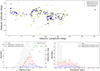 |
Fig. 1 Multi aspect analysis of observed cores: distribution, emission line detection rates, and distance distribution. Top panel: distribution of observed cores in the Galactic plane. The selected cores with and without detections of NH3 emission lines are denoted by blue and yellow circles, respectively. The red triangles denote Planck sources not only being part of our sample but having also been previously detected in ammonia by Fehér et al. (2022). Lower left: detection rate distribution of NH3 emission lines. The grey histogram represents the whole sample of 672 sources where we searched for NH3 lines. The red histogram represents the number of sources that we detected in the NH3 (1,1) line and the blue histogram refers to sources we also detected in the NH3 (2,2) line. The green triangles denote the detection rate for a given 857 µm flux density. Lower right: distribution of distances. Here the grey histogram also refers to the entire sample, while the red histogram visualizes those sources detected in NH3 (1,1). The blue histogram refers to sources we also detected in the NH3 (2,2) line. |
2.4 Data reduction
The data reduction was performed using the CLASS package of GILDAS1, and the python plot packages matplotlib (Hunter 2007). The NH3 data were spectrally smoothed to better compare and analyze these together with the CO data, resulting in a velocity resolution of 0.16km s−1. A feature was considered a genuine detection when the signal-to-noise ratio (S/N) was above 3. To convert hyperfine blended line widths to intrinsic line widths in the NH3 inversion spectrum (e.g., Barranco & Goodman 1998), we also fitted the averaged spectra using the GILDAS built-in “NH3 (1,1)” fitting method which can fit all 18 hyperfine components simultaneously. From this NH3 (1,1) fit we can obtain integrated intensity, line center velocity, intrinsic line widths of individual hyperfine structure (hfs) components, and optical depth (see Table A.2).
Main beam brightness temperatures TMB are obtained from GAUSS fit. Because the hyperfine satellite lines of the NH3 (2,2) transition are mostly weak, NH3 (2,2) optical depths are not determined. A single Gaussian profile was fitted to the main group of NH3 (2,2) hyperfine components. A total of eight NH3 cores were fitted with two velocity components. The spectral line of each distinguishable component was fitted with Gaussian and “NH3 (1,1)” fittings. These components are denoted by the labels “a” and “b” appended to the respective source names, as presented in Table A.2. We treated these two velocity components as separate entities (i.e., plotted them as two distinct cores). However, most of the cores in our observations required only a single velocity component fit. Physical parameters of the dense gas such as rotational temperature (Trot), kinetic temperature (Tkin), and NH3 column density  were derived (see Sects. 3.2 and 3.3). Figure 2 provides examples of reduced and calibrated spectra of NH3 (1,1), and (2,2) inversion lines. Examples for typical ammonia spectrum in different S/N are shown in Fig. B.1.
For the 12CO, 13CO and C18O spectra, peak main-beam brightness temperature, local standard of rest (LSR) velocities, and line widths have been obtained by fitting Gaussian profiles (see Table C.1). The excitation temperature for CO (Tex(CO)), 13CO opacity  , C18O opacity
  , 13CO column density
  , C18O column density
  , and hydrogen column density
  were also calculated (see Table C.2).
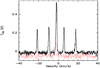 |
Fig. 2 Example for a typical ammonia spectrum. Shown are NH3 inversion lines from G092.26+03.8. The solid black line represents the observed NH3 (1,1) spectrum and the solid red line indicates the corresponding NH3 (2,2) profile. |
3 Sample properties
3.1 Distances
The distances of our sources were obtained from the literature (Wu et al. 2012; Planck Collaboration XXVIII 2016). For sources whose distances were unavailable in the literature, we employed the distance with the highest probability from the parallax-based distance estimator of the Bar and Spiral Structure Legacy Survey (Reid et al. 2016). The histogram of the kinematic distances is presented in the lower right panel of Fig. 1. It can be deduced from the distance distribution that the NH3 (1,1) detection rate is significantly increased beyond 0.6 kpc, and the NH3 (2,2) detection rate does not exhibit a clear correlation with distance. The distances of all sources range from 0.11 to 4.09 kpc, with a mean of 0.98 kpc and a median of 0.94 kpc. 56% of the sources have distances within 0.5 and 1.5 kpc.
3.2 Kinetic temperature
With the measured data, the rotational temperature (Trot), kinetic temperature (Tkin), NH3 column density  , thermal velocity dispersion σTherm, nonthermal velocity dispersion σNT, thermal-to-nonthermal pressure ratio Rp, thermal sound speed cs and Mach number (𝓜) of cores can be calculated.
Once the optical depth is determined by the “NH3 (1,1)” fitting as described in Sect. 2.4, we can calculate the excitation temperature of the NH3 (1,1) inversion transition through the relation (Ho & Townes 1983),
 (1)
(1)
where TMB and τ represent the temperature and the optical depth of the (1,1) line derived using the GILDAS built-in “GAUSS” and “NH3 (1,1)” fitting methods. A histogram of the optical depths of the (1,1) lines for our positions with NH3 (1,1) signal-to-noise ratios >3σ is summarized in Fig. 3b.
Since the relative populations of the K = 1 and 2 ladders of NH3 are not directly connected radiatively, they are highly sensitive to collisional processes. This allows us to use them as a thermometer of the gas kinetic temperature. The method described in Ho & Townes (1983), has been used to obtain the rotation temperature.
The rotation temperature is given by the expression
 (2)
(2)
where TMB (2,2) is the main beam brightness temperatures of the (2,2) line derived using the GILDAS built-in “GAUSS” fitting method.
We estimated the kinetic temperature Tkin using the approximation of Tafalla et al. (2004):
 (3)
(3)
where the energy gap between the (1,1) and (2,2) states is ∆E12= 41.5 K. This approximation has been derived with Monte Carlo models and provides an accuracy of 5% in the range between 5 and 20 K. Most of our sources can be found in this interval.
3.3 NH3 column density
Computing the ammonia column density requires the optical depth and line width of the (1, 1) inversion transition along with the rotational temperature, which is obtained from Eq. (2). As the optical depth and the rotational temperature depend only on line ratios, the resulting column density is a source-averaged quantity.
Realistically assuming that for our cold sources, the bulk of the ammonia populations resides in the metastable (J = K), (J, K) = (0, 0) to (3, 3) levels, the total NH3 column densities can be calculated from NH3 (1,1) following (Rohlfs & Wilson 2004),
 (4)
(4)
and
 (5)
(5)
where N(1,1) is the column density of the NH3 (1,1) transition, the FWHM line width ∆υ is in km s−1, the line frequency v is in GHz, and the rotational temperature Trot is in Kelvin.
3.4 Velocity dispersions, sound speed, and gas pressure ratio
The observed line widths provide a measure of the internal motions within each Planck source. Here we computed non-thermal velocity dispersion (σNT), thermal velocity dispersion (σTH), and sound speed (cs) following Levshakov et al. (2014), Tang et al. (2017, 2018a,b, 2021).
 (6)
(6)
where σv = ∆υ(1,1)/8 ln(2), and σTH = (kBTkin/17mH)1/2. mH is the mass of a single hydrogen atom, and kB is the Boltzmann constant.
The thermal sound speed can be calculated with
 (7)
(7)
where µ = 2.37 is the mean molecular weight for molecular clouds (Dewangan et al. 2016).
We also calculated the thermal-to-nonthermal pressure ratio ( ; Lada et al. 2003) and Mach number (given as 𝓜 = σNT/cs).
The statistical properties of the sample are summarised in Table 1 including the mean values and the medians of the derived quantities, as well as the minimal and maximal values. The derived values of Tex, Trot, Tkin, Ntot, σTH, σNT, cs, 𝓜 and RP for individual Planck sources are listed separately in Table A.2.
4 Results
4.1 NH3 detection rates
Out of the 672 Planck early cold cores (ECCs) that were surveyed with the Nanshan 26-m telescope for NH3, 249 sources (37%) were detected with NH3 (1,1) emission lines. Of these, 187 sources reveal NH3 (1,1) hyperfine structure, while 76 sources (11%) also show NH3 (2,2) emission lines. Observed parameters and calculated parameters are given in Tables A.2 and A.3.
The highest angular resolution of the Planck survey is 5 arcmin, at a frequency of 857 GHz. We plotted the distribution of observed sources and the NH3 lines detected in this work as well as the detection rate of the NH3 (1,1) line as a function of the 857 GHz aperture flux density S857 of the Planck Sources in the lower left panel of Fig. 1. We observe that sources with S857 larger than 3 Jy have a 100% detection rate. Furthermore, the detection rate of the NH3 (1,1) line increases from 0 to 100 percent as the flux density S857 rises from 1.5 to 4.6 Jy. However, it should be noted that while the detection rates of the NH3 (1,1) line are 100% in the last bins, the number of sources within these bins is limited, with only 8, 6, 4, 3, 2, and 2 sources in total.
In the lower right panel of Fig. 1, we observed an unexpectedly low detection rate of ammonia in regions with small kinematic distances. To understand this phenomenon, we performed a column density analysis of sources situated within a distance of less than 0.45 kpc. Utilizing hydrogen column density data from the Planck Collaboration XXIII (2011), we found a difference in column densities between sources where ammonia was detected and those where it was not, within this near distance (less than 0.45 kpc). Specifically, sources with detected ammonia exhibited an average hydrogen column density of 4.32 × 1021 cm−2, while those without ammonia detection had an average hydrogen column density of 1.99 × 1021 cm−2. Moreover, it is important to consider that sources in these nearby regions may have relatively extended spatial distributions. This spatial extension implies that during our observations of ammonia point sources, we may inadvertently miss the real peaks of the Planck cold cores.
The top panel of Fig. 1 presents the spatial distribution of the detected sources, which are mainly located in local star-forming regions such as Taurus and Orion and the galactic plane. This trend is shared by all of the ECCs and CO-selected cores in the sample (Wu et al. 2012; Yuan et al. 2016). As mentioned in Sect. 2.1, we cross-matched our sample with sources observed by Fehér et al. (2022), owing to distinct criteria detailed in Sect. 1. Consequently, there is a disparity in the distribution of sources across the galaxy between the two samples (see also Sect. 2.1).
4.2 Properties of the NH3 emitting gas
Figure 3 shows the statistics of observed and physical properties for the NH3 detected sample. The top left panel shows the intrinsic line width of an individual hfs component, ∆V (NH3 (1,1)), which ranges approximately from 0.36 to 2.36 km s−1, with an average of 0.89 ± 0.29 km s−1, which suggests that the nonthermal turbulence of these sources is significant (errors correspond to the standard deviations of the mean throughout this article). The top middle panel of Fig. 3 shows the sample optical depths, which range from 0.1 to 5.3 with an average value of 1.6, implying that NH3 (1,1) lines in most of the detected PGCC cores are optically thick (see Table 1).
The top right panel shows the excitation temperature, Tex, which ranges approximately from 2.8 to 5.4 K, with a mean and median of 3.2 and 3.1 K, respectively. The bottom left panel of Fig. 3 shows the derived rotational temperature, which exhibits a range of 8.6 to 17.6 K, with an average value of 11.4 ± 2.2 K. The median value of the rotational temperature is 10.7 K, with a typical value of approximately 10 K. Remarkably, 83% of the sources exhibit values lying between 8 and 14 K. The NH3 kinetic temperature distribution, illustrated in the bottom middle panel of Fig. 3, ranges from 8.9 to 20.7 K, with an average of 12.3 ± 2.9 K and a median value of 11.4 K. The total NH3 column density ranges from 0.36 to 6.07 × 1015 cm−2, with an average of 2.04 × 1015 cm−2. The total column densities of NH3 are presented as a histogram in the bottom right panel of Fig. 3, exhibiting a peak around 1015.4 cm−2 in our sample.
The thermal velocity dispersion of NH3 (1,1) lines detected at a >3σ level shows a range of 0.07 to 0.10 km s−1, with an average of 0.08 ± 0.01 km s−1 and a median of 0.07 km s−1. The nonthermal velocity dispersion of NH3 (1,1) for cores ranges from 0.30 to 1.09 km s−1, with an average of 0.55 ±0.18 km s−1 and a median of 0.49 km s−1. The thermal linewidth is significantly smaller than the nonthermal linewidth, which suggests that nonthermal motions dominate the dense gas in the PGCCs. The sound speed of the gas ranges from 0.18 to 0.27 km s−1, with an average of 0.21 ± 0.02 km s−1 and median of 0.20 km s−1. The thermal to nonthermal pressure ratio in the gas traced by NH3 (1,1) ranges from 0.01 to 0.06, with an average of 0.02 ± 0.01, and a median of 0.02. The Mach number ranges from 1.6 to 5.0 with an average of 2.7 ± 0.8, and a median of 2.5.
4.3 Thermal and nonthermal motions
The clumps are supported against their gravity by both thermal and nonthermal motions (Cho & Lazarian 2003). The former is a manifestation of the kinetic temperature within a clump, while the latter originates from star-forming activities such as infall motions and outflows that can broaden the nonthermal velocity dispersion. However, the quiescent nature of PGCCs suggests that these motions are not particularly vigorous. Therefore, turbulent motion is the primary contributor to the nonthermal motion of these cores. Ammonia is one of the few dense gas tracers that allows for the simultaneous computation of line width and kinetic temperature, as well as thermal and nonthermal line widths. Our data are particularly well-suited for investigating these two types of motion.
When turbulent energy is converted into heat, a correlation is expected to exist between the kinetic temperature and linewidth (Guesten et al. 1985; Molinari et al. 1996; Ao et al. 2013; Ginsburg et al. 2016; Immer et al. 2016; Tang et al. 2017, 2018a,b, 2021). In this study, we investigate the existence of a correlation between temperature and turbulence in PGCCs traced by the dense gas. To achieve this, we utilized the NH3 (1,1) and (2,2) line ratio derived kinetic temperature and NH3 nonthermal velocity dispersion (σNT) as a decent approximation proxy for turbulence. The nonthermal velocity dispersions versus the kinetic temperature for the sources are shown in Fig. 4, with the dotted line representing the thermal sound speed. Our results indicate a weak correlation between nonthermal velocity dispersion and kinetic temperature, suggesting that turbulent heating may contribute to gas temperature in these cold cores.
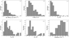 |
Fig. 3 Histograms of physical parameters derived from NH3. (a) Intrinsic line widths of individual NH3 (1,1) hyperfine structure components with hyperfine structure and a peak line flux threshold of 3σ; (b) peak optical depths of the main group of hf components τm (1,1) for those positions with NH3 (1,1) hyperfine structure and S/N > 3 (these line widths and peak optical depths are derived from the GILDAS built-in “NH3 (1,1)” fitting method); (c) excitation temperature Tex; (d) rotational temperature Trot; (e) kinetic temperature Tkin; (f) NH3 column densities. |
NH3 parameters of our sample of PGCC cores.
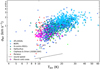 |
Fig. 4 Nonthermal velocity dispersion σNT vs. gas kinetic temperature derived from NH3 (1,1). The black dotted line at the bottom represents the thermal sound speed. |
Numbers of associated stellar objects.
Matching results by types of stellar objects.
4.4 Associated stellar objects
The associated objects of the cores are crucial for our understanding of their environment and evolutionary stages. Therefore, we investigated the objects associated with the cores, including infrared (IR) objects, young stellar objects (YSOs), and young stellar object candidates (YSO candidates). We obtained the stellar objects from the Simbad website. Statistical properties are given in Tables 2 and 3. YSOs are distinguished by their manifestation of not only infrared excess but also additional spectral features, providing evidence of active star formation processes (Allen et al. 2004; Gutermuth et al. 2004). Conversely, YSO candidates represent potential YSOs necessitating further scrutiny and validation.
In our study, we adopted the ammonia beam size (~2′) as a matching criterion. Among the 672 cores observed, our analysis revealed the presence of 131 (~19%) IR objects, 57 (~8%) YSOs and 58 (~ 8%) YSO candidates. The rare association may indicate low star formation activity (Lada et al. 2009; Lombardi et al. 2010). However, it cannot be entirely excluded that the associated objects originate from different gas clumps located along the line-of-sight (Wu et al. 2006). It is important to note that certain cores in our sample may encompass multiple IR sources, as well as multiple YSOs or YSO candidates. Notably, the majority of these IR objects correspond to single-point sources detected by the infrared astronomical satellite (IRAS). Overall, our findings indicate that 149 (~22%) cores have different types of associated objects within a beam size of ~2′. Additionally, we find that 112 (~17%) cores contain at least one IR object, 29 (~4%) cores have YSOs, and 23 (~3%) cores contain YSO candidates. Among these, 102 sources only associate with IR objects, 18 cores only associate with YSOs and 16 cores only associate with YSO candidates. Four cores are associated with both YSOs and YSO candidates, seven cores with both YSO and IR objects, and three cores with both IR objects and YSO candidates.
Considering the 249 cores where NH3 (1,1) emission was detected, we find 66 (~27%) IR objects, 48 (~19%)YSOs, and 52 (~21%) YSO candidate sources associated with these cores using the aforementioned ~2′ criterion. In general, 80 (~32%) cores have different types of associated objects. Additionally, we find that 53 (~21%) cores contain at least one IR object, 23 (~9%) cores host YSOs, and 17 (~7%) cores harbor YSO candidates. Forty-five sources only associate with IR objects, 13 cores only associate with YSOs and nine cores only associate with YSO candidates. Five cores are associated with both YSOs and YSO candidates, five cores with both YSOs and IR objects, and three cores with both IR objects and YSO candidates.
Based on preliminary statistical analysis, the proportion of sources with NH3 emission matching IR sources and stellar objects is higher than the overall proportion of the total sample matching IR sources and YSOs. The ammonia detection rate of sources matching young stellar objects or their candidates in the 672 observed cores is 66%, while the ammonia detection rate of sources matching IR objects is 45%. The ammonia detection rate is higher in sources with matching stellar objects. Not all sources with matched stellar objects and IR objects have been detected in NH3 (1,1). There can be several reasons for this. Firstly, distance plays a significant role. If the YSOs or IR objects are located at a large distance, the faint emission signal from ammonia may be too weak to be detected. Secondly, the spatial resolution of the observing instrument can also be a factor. Other factors include line-of-sight effects and environmental conditions, where the physical environment surrounding the YSOs may influence the presence of ammonia molecules. The inescapable issue at hand is that our matching could potentially be limited to line-of-sight coincidence, lacking the necessary distance information for spatial alignment.
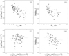 |
Fig. 5 Correlations of NH3 and 13CO column densities and fractional abundances with kinetic temperature and hydrogen column density. (a,b) Column densities and fractional abundances NNH3/NH2(13CO) versus kinetic temperature Tkin and (c,d) vs. the column density of H2 derived from 13CO |

4.5 NH3 abundances
The column densities of ammonia in our sample range from 0.36 ~ 6.07 × 1015 cm−2, with a mean value of approximately 2.04 × 1015 cm−2 and a median value of about 1.83 × 1015 cm−2 (Table 1). We utilized 13CO to derive the H2 column densities as described in Appendix C. The H2 column densities  (13CO) range from 7.0 × 10²⁰ to 2.88 × 1022 cm−2, with an average of 7.4 × 1021 cm−2. The column densities of NH3 denoted as
  , were compared with the column densities of H2, denoted as
  , derived from 13CO to determine the fractional abundance of ammonia in each source. The fractional abundance, χNH3, is defined as the ratio of
  to
to  (13CO). The ammonia abundances in the sources range from 0.3 to 9.7 × 10⁻⁷, with an average of 2.7 × 10⁻⁷.
Figure 5 illustrates the column densities of NH3 and its abundances,; χNH3, as a function of H2 column density and kinetic temperature Tkin. It is observed that the NH3 column densities and fractional abundances are inversely proportional to the kinetic temperatures. Moreover, there is a trend of decreasing fractional NH3 abundance,; χNH3, with increasing  .
.
5 Discussion
5.1 Column densities and abundances
The ammonia column densities in our results are consistent with the findings of PGCC selected sources from SCUBA-2, whose column densities range from 0.4 to 1.5 × 1016 cm−2, with a mean value of approximately 1.3 × 1015 cm−2 (Fehér et al. 2022). The ammonia column densities we obtained in our observations are also consistent with those reported in most star-forming environments (Dunham et al. 2011; Wienen et al. 2012; Cyganowski et al. 2013).
The average value of  (13CO), 7.4 × 1021 cm−2, is consistent with the results obtained from the Planck cold cores observed by PMO (Wu et al. 2012; Meng et al. 2013; Zhang et al. 2016). In the SCOPE-2 follow-up observations, the H2 column densities of 97 Planck cold cores range from 1022 to 1024 cm−2 (Fehér et al. 2022), which are higher than the column densities obtained in our work. This may be attributed to the fact that the SCOPE-2 survey does not include sources with column densities
  (Eden et al. 2019).
Previous observations of NH3 fractional abundance in high-mass star-forming clumps suggest a median value of 2.7 × 10⁻⁸ (Urquhart et al. 2015). Additionally, Dunham et al. (2011), Wienen et al. (2012), and Merello et al. (2019) obtained average abundance values of 1.2 × 10⁻⁷, 4.6 × 10⁻⁸, and 1.5 × 10⁻⁸, respectively, in clumps of the Bolocam Galactic Plane Survey (BGPS), the APEX Telescope Large Area Survey of the GALaxy (ATLASGAL), and the Hi-GAL survey. Furthermore, fractional abundances of 4 × 10⁻⁸, 8 × 10⁻⁷ and 1 × 10⁻⁸ were derived for infrared dark clouds by Pillai et al. (2006), Ragan et al. (2011), and Chira et al. (2013), respectively. The average NH3 abundance derived from PGCCs in this study is one order of magnitude greater than that of MSF regions and IRDCs and exhibits a narrow distribution similar to that of IRDCs. The elevated NH3 fractional abundance in PGCCs relative to other star-forming regions is likely attributable to the earlier phase of cloud evolution of PGCCs compared to massive star-forming (MSF) regions or even IRDCs. Ammonia is more abundant in cold, dense cores than most other molecules (Bergin & Langer 1997). The average NH3 abundances obtained in our study are consistent with those predicted for low-mass pre-protostellar cores by chemical models (Bergin & Langer 1997).
The NH3 column densities and fractional abundances are inversely proportional to the kinetic temperatures (see in Figs. 5a,b), which is consistent with the findings of previous studies on infrared dark clouds (Chira et al. 2013). The NH3 column densities in all cores tend to increase with  , as shown in Fig. 5c, following the general trend that the NH3 emission follows the dust continuum emission in the cores. This is in agreement with the results reported by Ragan et al. (2011), who found that IRDCs with no evidence of embedded star formation activity exhibit a strong correlation between ammonia and H2 column density. A similar trend is observed in the cold cores in our observation.
Fundamental information on different NH3 samples.
5.2 Comparative analysis of thermal and nonthermal motions
To obtain comprehensive statistics on PGCCs, we conducted a comparative analysis of the nonthermal velocity dispersions and kinetic temperatures. Studies encompass a diverse range of samples, including high-mass star-forming clumps at various evolutionary stages from ATLASGAL and BGPS surveys (Dunham et al. 2011; Wienen et al. 2012), high contrast infrared dark clouds (IRDCs; Chira et al. 2013), as well as starless cores in the Perseus region (Rosolowsky et al. 2008; Schnee et al. 2009), and dense cores in the Ophiuchus, Cepheus, and Orion L1630 and L1641 molecular clouds (Harju et al. 1991, 1993; Friesen et al. 2009). This comprehensive approach allows us to gain valuable insights into the physical properties of these objects and their evolutionary characteristics. In Table 4, we have compiled a list containing the fundamental information of the sources used for comparison in this study.
As seen in Fig. 4, unlike high-mass star-forming clumps and dense cores in star-forming regions (Dunham et al. 2011; Wienen et al. 2012), the relationship between nonthermal velocity dispersion and kinetic temperatures in PGCCs is much weaker. Additionally, the distribution of nonthermal velocity dispersion and kinetic temperatures of Planck cold cores is narrower when compared to the observations of the other samples. Spearman’s rank correlation coefficients (ρ) for nonthermal velocity dispersion versus kinetic temperatures in different samples and the resultant ρ-values are presented in Table D.1. The table presents the obtained ρ-values along with their corresponding P-values. The analysis of this table reveals varying degrees of correlation between nonthermal velocity dispersion and kinetic temperature across different samples. Particularly, a conspicuous positive correlation is discernible in the ATLASGAL, BGPS, Ophiuchus, Cepheus, and Orion L1630/L1641 samples, underscored by small P-values. However, in the High-contrast IRDCs, the correlation is relatively weak, with a Spearman correlation coefficient of 0.07 and a P-value of 0.45, suggesting a weak and nonsignificant linear relationship between these two variables. The Perseus sample also manifests a relatively weak correlation, featuring a Spearman correlation coefficient of 0.2 and a P-value of 0.16, implying a modest positive correlation trend that lacks statistical significance. In contrast, our Planck cold cores sample displays a pronounced positive correlation between nonthermal velocity dispersion and kinetic temperature. With a Spearman correlation coefficient of 0.33 and a P-value of 4.00 × 10⁻³.
Furthermore, gas pressure ratios derived from our results closely align with those obtained by Urquhart et al. (2015), who conducted a study on 66 massive young stellar objects and compact Hii regions from the RMS survey (red MSX source survey, Lumsden et al. 2013). Urquhart et al. (2015) obtained gas pressure ratios (Rp) of 0.01–0.02 for both massive star-forming and quiescent clumps. In contrast, Lada et al. (2003) reported significantly higher values of Rp = 4–5 for low-mass star-forming cores, such as Barnard 68, based on C18O and C34S data. Our sample, which includes nonthermal movements that significantly contribute to the kinetic energy balance, more closely aligns with samples of massive clumps compared to others.
5.3 Correlation between NH3 and other molecular species
In their survey of 674 Planck cold clumps, Wu et al. (2012) discovered that the velocities of transitions from CO and its isotopologues were highly consistent with one another. We plot the absolute value of the difference between J = 1−0 transitions of 13CO and C18O and the NH3 (1,1) line-center velocities from Gaussian fits in Figs. 6a,b. When multiple 13CO velocities were detected along the line of sight, we assumed that the velocity component closest to the NH3 velocity is associated with the core (Kirk et al. 2007). A total of eight NH3 cores were fitted with two velocity components. These components are denoted by the labels “a” and “b” appended to the respective source names, as presented in Table A.2. We treated these two velocity components as separate entities (i.e., plotted them as two distinct cores).
The minute discrepancy in centroid velocity between NH3 and 13CO (~0.17 km s−1), and between NH3 and C18O (~0.18 km s−1), can be compared to the distinction in line-center velocities of N2H+ and C18O in low-mass, starless, and protostellar cores Walsh et al. (2004); Kirk et al. (2007). Figures 6a,b illustrate that the majority of cores (64% for the difference between 13CO NH3 (1,1) line-center velocities and 70% for the difference between C18O and NH3 (1,1) line-center velocities) exhibit differences smaller than the sound speed (dotted lines), and the remaining cores have differences that are not much larger. This phenomenon was investigated in the Perseus molecular cloud by Kirk et al. (2007), who found that the relative motions of dense N2H+ cores and their envelopes (measured in C18O) generally exhibit velocity differences lower than thermal motions in the majority of cases (~90%). This is also consistent with the findings of Walsh et al. (2004), who measured a core-to-envelope velocity difference that exceeded the sound speed in only 3% of their sample. These samples consisted of isolated low-mass cores. Therefore, these comparisons suggest that the velocity differences between low and high-density tracers in the Planck cores observed by NH3 are similar to those in low-mass, starless, or prestellar cores. In the survey of CO-selected cores in Planck cold clumps, Yuan et al. (2016) found that the central velocity differences of transitions from 13CO, HCO+ and HCN are strikingly consistent with each other. The central velocities (obtained by fitting Gaussian profiles) between 13CO and HCO+  , 13CO and
  and
and  in their study have mean values of 0.006, 0.05, and 0.002 km s−1, respectively. The smaller deviations from Yuan et al. (2016) may indicate that 13CO, HCO+, and HCN are better coupled with each other. It is important to note that the channel spacing employed in their study was 0.21 km s−1. In this work, the mean value of the velocity difference among the central velocities of 13CO and NH3 is 0.17 km s−1, with channel spacing of 0.16 km s−1. It is worth noting that the relatively low-velocity resolution might impact the interpretation of the small velocity differences observed in both cases, To address this, future observations with higher resolution would be beneficial for a more accurate comparison. By improving the velocity resolution, we can measure and compare the central velocity differences between different molecular lines more accurately, providing deeper insights. Such observations would help further validate and explain the consistency among these molecular transitions and enhance our understanding of the physical processes occurring within Planck cold clumps. Therefore, future high-resolution observations would help to further validate this matter.
The mean intrinsic line width of the NH3 (1,1) lines obtained from GAUSS fit is approximately 0.89 km s−1, which is comparable to that of C18O J = 1–0 (0.8 km s−1) in Wu et al. (2012), C2H N = 1–0 (1.0 km s−1) reported in Liu et al. (2019), and HCN J = 1–0 (1.06 km s−1) in Yuan et al. (2016). The differences in line widths among different molecular tracers may result from turbulence at different scales. Figures 6c,d show the distributions of the differences in line widths between 13CO and C18O with NH3. The mean widths of NH3 and 13CO are nearly identical, with an average difference of ~0.14 km s−1. In contrast to high-mass star-forming clumps, where the average difference between NH3 and 13CO is 4.3 km s−1 (Wienen et al. 2012), the intrinsic line widths of NH3, 13CO and C18O are approximately equal in our sample. This finding is consistent with the notion that these PGCCs are quiescent, as the majority of them appear to be transitioning from clouds to dense cores (Wu et al. 2012).
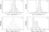 |
Fig. 6 Distributions between differences of line-center velocities (a, b) and line widths (c, d) of 13CO, C18O and NH3. The average sound speed is indicated as dotted lines (a, b). |
5.4 A comparison with different star formation samples
To investigate the physical conditions and assess the potential for star formation within the cold clumps, we conducted a comparative analysis of various NH3 molecular line surveys targeting different types of celestial objects. This analysis involved a comprehensive examination of line widths, kinetic temperatures, NH3 column densities, as well as column densities of H2, and fractional abundances. In this particular study, to conduct a more comprehensive comparative analysis, we have incorporated not only the samples mentioned in Sect. 4.3, but also included additional statistical samples, ultra-compact Hii (UC Hii) regions or UC Hii region candidates (Molinari et al. 1996), high infrared (IR) extinction clouds (Rygl et al. 2010) and extended green objects (EGOs; Cyganowski et al. 2013). The fundamental information regarding these sources has been presented in Table 4. It is crucial to emphasize that not all papers provide data for every parameter. In certain studies, some parameters were not reported. Therefore, in the comparison involving these parameters, we opted to consider only those papers that presented available data.
The kinetic temperatures of the cores range from 8.9 to 20.7 K, with an average of 12.3 ± 2.9 K and a median value of 11.4 K (as mentioned in Sect. 4.2), and after cross-matching our NH3 detected 249 sources with PGCCs from Planck Collaboration XXVIII (2016), we have observed that the dust temperature (Tdust) of these 249 sources falls within the range of 8.6 to 13.9 K, with an average value of 11.5 K. The similarity in temperature ranges between Tkin and Tdust indicates an efficient coupling of gas and dust. The cumulative distribution of the kinetic temperature of NH3 for different samples is presented in Fig. 7a. The results indicate that the UC Hii candidates exhibit the highest kinetic temperatures (Molinari et al. 1996), while the Planck cold cores show lower temperatures compared to other classes of sources. The temperature distribution of the samples is distinct and follows the expected evolutionary sequence. Hence, the kinetic temperature can serve as a reliable indicator for distinguishing between different evolutionary stages.
Figure 7b depicts the cumulative distribution of NH3 (1,1) line widths. Our analysis indicates that the line widths of ATLASGAL sources are the largest. The changes in the ATLAS-GAL and UC Hii regions flatten off when the line width exceeds ~2.5 km s−1, and their slopes are nearly identical when the line width is smaller than 2.5 km s−1. The variation of the cumulative fraction function of line width for the Planck cold cores is narrower when compared to other star-forming samples (Dunham et al. 2011; Wienen et al. 2012; Chira et al. 2013), and exhibits a similar cumulative distribution figure to those found in the dense cores of regions such as Cepheus, and Orion L1630 and L1641, and Ophiuchus, as reported in Harju et al. (1991, 1993) and Friesen et al. (2009). However, the average linewidth in the Planck cold cores is slightly larger than that observed in Ophiuchus (0.62 km s−1). Notably, the higher line width values observed in the Planck cold cores, in comparison to the dense cores in Ophiuchus, may imply that they are in more advanced and warmer stages of evolution. However, it is worth highlighting that the line width remains relatively small across the various samples under examination. Figures 7c–e present the cumulative distribution of column densities for NH3, H2, and fractional ammonia abundances for various samples. The ammonia column densities of cold cores are generally higher than those of other samples and are even comparable to those of ATLAS-GAL and EGO sources. Conversely, the cumulative distribution for Planck cold clumps exhibits the smallest H2 column density range, resulting in high ammonia abundances. Despite the relatively high NH3 column density observed in Planck cold cores, comprehensive consideration of its lower temperature, linewidth, and other parameters still leads to the conclusion that Planck sources are in an early stage of evolution.
To quantitatively compare the distributions, we conducted two-sample Kolmogorov–Smirnov (K–S) tests using the procedure in the scipy package2. This statistical test assesses the dissimilarity between two samples, with the K–S statistic serving as a measure of this dissimilarity, ranging from 0 to 1. A K–S statistic of 0 implies that there is no significant difference, suggesting the two samples may be from the same distribution. Conversely, a higher K–S statistic suggests a lower likelihood of the samples originating from the same distribution. Additionally, we computed P-values for each pair of samples, small P-values provide compelling evidence that the observed samples are drawn from distinct populations. The outcomes of these tests are summarized in Table D.2. In summary, the K–S test results for all examined parameters, including kinetic temperature, line width, ammonia column density, hydrogen molecule column density, and ammonia abundance, consistently yielded P-values below 0.05. These findings strongly imply substantial disparities between the Planck cold cores and the comparison samples in the examined parameters, which may reflect variations in their physical properties or the influence of distinct environmental conditions. Nevertheless, it is noteworthy that, in the distributions of kinetic temperature and linewidth, the Perseus, Cepheus, and Orion L1630/L1641 samples exhibit smaller K–S statistic values. Moreover, their P-values are comparatively larger than those of other samples. The K–S test results for the kinetic temperature and line width of the Planck cold cores, starless and dense cores do not contradict that they are drawn from the same parent population. The comparison of the ammonia column density distribution using the K–S test yields that these samples are measurably different. Additionally, in the abundance distribution, Planck displays relatively smaller K–S values and larger P-values when compared to BGPS and ATLASGAL samples.
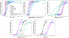 |
Fig. 7 Comparisons for the cumulative distribution of the line widths of NH3 (1,1), kinetic temperatures, column densities, and abundances of different star formation samples. In the comparison involving these parameters, we opted to consider only those papers that presented available data. |
6 Summary
We used the Nanshan 26-m radio telescope to perform single-pointing observations of NH3 (1,1) and (2,2) inversion transitions toward 672 Planck sources. The main results of this study are as follows:
Among the observed 672 Planck sources, 249 (37%) were detected. In these detections, 187 cores exhibit NH3 (1,1) hyperfine structure while 76 (11%) cores also show corresponding NH3 (2,2) emission lines. The observed sources are mainly located in local star-forming regions. The detection rate of NH3 is positively correlated with the continuum emission fluxes of Planck sources at a frequency of 857 GHz, increasing as the 857 GHz flux density increases.
Among the observed 672 sources, ~22% have associated stellar and IR objects within the beam size (~2′). This may indicate low star formation activity of the cores in our sample and the ammonia detection rate is higher in sources with matching stellar objects.
The correlation between thermal and nonthermal velocity dispersion in NH3 (1,1) indicates the dominance of non-thermal pressure and supersonic nonthermal motions in the dense gas traced by NH3. In contrast to high-mass star-forming clumps and dense cores in star-forming regions, the relationship between nonthermal velocity dispersion and kinetic temperatures in PGCCs is notably weaker, with lower values observed for both parameters relative to other samples under our examination.
The comparison of the line-center velocities of NH3 with those from 13CO and C18O reveals small discrepancies (0.17 ± 0.33 km s−1, 0.12 ± 0.18 km s−1). The widths of NH3, 13CO, and C18O in our sample were almost undistinguishable. These are consistent with the idea that these PGCCs are quiescent, as the majority of them appear to be transitioning from clouds to dense clumps.
The ammonia column densities range between 0.36 to 6.07 × 1015 cm−2. The mean value is approximately 2.04 ×1015 cm−2, and the fractional abundances of ammonia range from 0.3 to 9.7 × 10⁻⁷, with an average of 2.7 × 10⁻⁷. Our observed fractional abundances of NH3 are consistently one order of magnitude larger in PGCCs than in massive star-forming (MSF) regions and infrared dark clouds (IRDCs). This significant difference in NH3 fractional abundance suggests that PGCCs are in an earlier phase of cloud evolution compared to MSF regions and IRDCs. The elevated NH3 fractional abundance in PGCCs relative to other star-forming regions is likely attributable to the earlier phase of cloud 1evolution of PGCCs compared to MSF regions or even IRDCs.
The kinetic temperatures of the cores range from 8.9 to 20.7 K, with an average of 12.3 ± 2.9 K. Similar temperature ranges between Tkin and Tdust indicate that the gas and dust are well coupled.
The cumulative distribution shapes of line widths in the Planck cold cores closely resemble those of the dense cores found in regions Cepheus, and Orion L1630 and L1641, but with slightly higher values compared to Ophiuchus. However, the higher line width values in the Planck cold cores, when compared to these dense cores in Ophiuchus, suggest that they might be in more advanced and warmer stages of evolution. Nevertheless, it is worth noting that line width values remain small across the various samples under examination. This observation highlights the unique characteristics of the Planck cold cores in the context of their evolutionary stages.
Acknowledgements
This work was mainly funded by the National Key R&D Program of China under grant no. 2022YFA1603103. It was also partially funded by the Regional Collaborative Innovation Project of Xinjiang Uyghur Autonomous Region grant 2022E01050, the Tianshan Talent Program of Xinjiang Uygur Autonomous Region under grant No. 2022TSYCLJ0005, the Natural Science Foundation of Xinjiang Uygur Autonomous Region under grant Nos. 2022D01E06 and 2022D01A362, the Chinese Academy of Sciences (CAS) “Light of West China” Program under grant nos. xbzg-zdsys-202212, 2020-XBQNXZ-017, and 2021-XBQNXZ-028, the National Key R&D Program of China with grant 2023YFA1608002, the National Natural Science Foundation of China (NSFC) under grants nos. 12173075, 12373029, and 12103082, the Xinjiang Key Laboratory of Radio Astrophysics under grant No. 2023D04033, the Youth Innovation Promotion Association CAS, and the Tianchi Talent Program of Xinjiang Uygur Autonomous Region. C.H. has been funded by the Chinese Academy of Sciences President’s International Fellowship Initiative by grant No. 2023VMA0031. Moreover, this work is sponsored (in part) by the Science Committee of the Ministry of Science and Higher Education of the Republic of Kazakhstan grant no. AP13067768. This work is based on observations made with the Nanshan 26-m radio telescope, the Nanshan 26-m Radio Telescope is partly supported by the Operation, Maintenance and Upgrading Fund for Astronomical Telescopes and Facility Instruments, budgeted from the Ministry of Finance of China (MOF) and administrated by the Chinese Academy of Sciences (CAS), and the Urumqi Nanshan Astronomy and Deep Space Exploration Observation and Research Station of Xinjiang.
Appendix A ECC Clump Catalogue
Basic information of the observed sources
Observed parameters of the NH3 (1,1) and NH3 (2,2) emission lines in the NH3 detected sources.
Calculated parameters of the NH3 (1,1) and (2,2) emission lines detected in the 73 cores.
Appendix B Samples of NH3 spectra
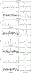 |
Fig. B.1 Examples for typical ammonia spectra in different S/N. Spectra include NH3 (1,1) and (2,2), 12CO, 13CO and C18O (1-0) transitions toward cores, namely G070.44-01.54, G110.65+09.65, G158.22-20.14, and G160.51-16.84. The green color indicates the NH3 (1,1) fitting and Gauss fitting of NH3 (2,2), 12CO, 13CO and C18O profile. |
Appendix C Derived CO parameters
Our calculations assume that the cores are in a state of local thermodynamical equilibrium (LTE) and the 13CO emission is optically thin. Adopting a beam-filling factor of unity, the excitation temperature for CO is derived from the following equation (Pineda et al. 2010; Kong et al. 2015)
![Mathematical equation: ${T_{{\rm{ex (CO)}}}} = 5.33{\left\{ {\ln \left[ {1 + {{5.33} \over {\left( {{{\rm{T}}_{{\rm{mb}}{,^{12}}{\rm{CO}}}} + 0.818} \right)}}} \right]} \right\}^{ - 1}}{\rm{K}},$](/articles/aa/full_html/2024/04/aa48381-23/aa48381-23-eq34.png) (C.1)
(C.1)
where  is the peak intensity of 12CO (J = 1−0) in units of K. We then obtain the optical depths, τ, and the column densities,
  for the 13CO and C18O molecules using the following equations (Lada et al. 1994; Kawamura et al. 1998).
![Mathematical equation: ${\tau _{13}}_{_{{\rm{CO}}}} = - \ln \left\{ {1 - {{{T_{{\rm{mb}}{,^{13}}{\rm{CO}}}}} \over {5.29\left( {\left[ {\exp {{\left( {5.29/{T_{{\rm{ex}}({\rm{CO}})}} - 1} \right]}^{ - 1}} - 0.164} \right)} \right.}}} \right\},$](/articles/aa/full_html/2024/04/aa48381-23/aa48381-23-eq37.png) (C.2)
(C.2)
![Mathematical equation: ${\tau _{{{\rm{C}}^{18}}{\rm{O}}}} = - \ln \left\{ {1 - {{{T_{{\rm{mb}},{{\rm{C}}^{18}}{\rm{O}}}}} \over {5.27\left( {\left[ {\exp {{\left( {5.27/{T_{{\rm{ex}}({\rm{CO}})}} - 1} \right]}^{ - 1}} - 0.166} \right)} \right.}}} \right\},$](/articles/aa/full_html/2024/04/aa48381-23/aa48381-23-eq38.png) (C.3)
(C.3)
 (C.4)
(C.4)
and
 (C.5)
(C.5)
where  and
and  are peak intensities in K, while
  and
and  are the FWHM inewidths in km s−1. In the calculation, the excitation temperatures of 13CO have been assigned to be equal to those of 12CO. This would be reasonable when considering the fact that 12CO, 13CO, and C18O are well coupled in ECCs (Wu et al. 2012). Molecular hydrogen column densities were calculated by the fractional abundances of [H2]/[13CO] = 89 × 104 (McCutcheon et al. 1980) and [H2]/[C18O] = 7 × 10⁶ (Frerking et al. 1982) in the solar neighborhood.
We find that the hydrogen column density  values derived from 13CO and C18O are quite close to each other, suggesting that both 13CO and C18O are optically thin and the optical depth effect can be ignored in our calculation (Meng et al. 2013). Therefore we use 13CO to calculate
  , as listed in Table C.2 of Appendix C.
The excitation temperatures of CO J = 1−0 (Tex(CO)) for our cores range from 4.4 to 19.7 K. The mean value of Tex(CO)) is 10.5 K and it is smaller than the value in Wu et al. (2012) and the average dust temperature (13 K) for C3POs (Planck Collaboration I 2011). The H2 column densities  (13CO) of our cores are derived from
  covering the range of (0.07−2.88) × 1022cm−2 with a mean value of 7.4 × 1021 cm−2. Sources in our sample have similar
  column densities to those in Galactic second quadrant samples, with a mean value of 8 × 1021 cm−2 (Meng et al. 2013).
Parameters derived from the 12CO, 13CO, and C18O (1-0) lines.
Derived parameters of CO lines.
Appendix D Statistical analyses of different star formation samples
Spearman correlation of kinetic temperature versus nonthermal velocity dispersion in different star formation samples.
Kolmogorov-Smirnov test results for line widths, kinematic temperatures, column densities, and abundances distributions in different star formation samples. In the test, we only consider parameters that are presented in samples.
References
- Aguirre, J. E., Ginsburg, A. G., Dunham, M. K., et al. 2011, ApJS, 192, 4 [Google Scholar]
- Allen, L. E., Calvet, N., D’Alessio, P., et al. 2004, ApJS, 154, 363 [Google Scholar]
- André, P., Men’shchikov, A., Bontemps, S., et al. 2010, A&A, 518, A102 [Google Scholar]
- Ao, Y., Henkel, C., Menten, K. M., et al. 2013, A&A, 550, A135 [NASA ADS] [CrossRef] [EDP Sciences] [Google Scholar]
- Barranco, J. A., & Goodman, A. A. 1998, ApJ, 504, 207 [Google Scholar]
- Bergin, E. A., & Langer, W. D. 1997, ApJ, 486, 316 [Google Scholar]
- Bergin, E. A., & Tafalla, M. 2007, ARA&A, 45, 339 [Google Scholar]
- Chira, R.-A., Beuther, H., Linz, H., et al. 2013, A&A, 552, A40 [NASA ADS] [CrossRef] [EDP Sciences] [Google Scholar]
- Cho, J., & Lazarian, A. 2003, Rev. Mex. Astron. Astrofis. Conf. Ser., 15, 293 [Google Scholar]
- Cyganowski, C. J., Koda, J., Rosolowsky, E., et al. 2013, ApJ, 764, 61 [NASA ADS] [CrossRef] [Google Scholar]
- Dame, T. M., Hartmann, D., & Thaddeus, P. 2001, ApJ, 547, 792 [Google Scholar]
- Danby, G., Flower, D. R., Valiron, P., et al. 1988, MNRAS, 235, 229 [NASA ADS] [CrossRef] [Google Scholar]
- Dewangan, L. K., Ojha, D. K., Luna, A., et al. 2016, ApJ, 819, 66 [CrossRef] [Google Scholar]
- Dunham, M. K., Rosolowsky, E., Evans, N. J., II, et al. 2011, ApJ, 741, 110 [NASA ADS] [CrossRef] [Google Scholar]
- Eden, D. J., Liu, T., Kim, K.-T., et al. 2019, MNRAS, 485, 2895 [NASA ADS] [CrossRef] [Google Scholar]
- Evans, N. J., II 1999, ARA&A, 37, 311 [NASA ADS] [CrossRef] [Google Scholar]
- Fehér, O., Tóth, L. V., Kraus, A., et al. 2022, ApJS, 258, 17 [CrossRef] [Google Scholar]
- Frerking, M. A., Langer, W. D., & Wilson, R. W. 1982, ApJ, 262, 590 [Google Scholar]
- Friesen, R. K., Di Francesco, J., Shirley, Y. L., et al. 2009, ApJ, 697, 1457 [NASA ADS] [CrossRef] [Google Scholar]
- Ginsburg, A., Henkel, C., Ao, Y., et al. 2016, A&A, 586, A50 [NASA ADS] [CrossRef] [EDP Sciences] [Google Scholar]
- Guesten, R., Walmsley, C. M., Ungerechts, H., et al. 1985, A&A, 142, 381 [NASA ADS] [Google Scholar]
- Gutermuth, R. A., Megeath, S. T., Muzerolle, J., et al. 2004, ApJS, 154, 374 [NASA ADS] [CrossRef] [Google Scholar]
- Goldreich, P., & Kwan, J. 1974, ApJ, 189, 441 [CrossRef] [Google Scholar]
- Harju, J., Walmsley, C. M., & Wouterloot, J. G. A. 1991, A&A, 245, 643 [NASA ADS] [Google Scholar]
- Harju, J., Walmsley, C. M., & Wouterloot, J. G. A. 1993, A&AS, 98, 51 [NASA ADS] [Google Scholar]
- Ho, P. T. P., & Townes, C. H. 1983, ARA&A, 21, 239 [NASA ADS] [CrossRef] [Google Scholar]
- Hunter, J. D. 2007, Comput. Sci. Eng., 9, 90 [NASA ADS] [CrossRef] [Google Scholar]
- Immer, K., Kauffmann, J., Pillai, T., et al. 2016, A&A, 595, A94 [NASA ADS] [CrossRef] [EDP Sciences] [Google Scholar]
- Jijina, J., Myers, P. C., & Adams, F. C. 1999, ApJS, 125, 161 [Google Scholar]
- Juvela, M., Ristorcelli, I., Montier, L. A., et al. 2010, A&A, 518, L93 [NASA ADS] [CrossRef] [EDP Sciences] [Google Scholar]
- Juvela, M., Ristorcelli, I., Pagani, L., et al. 2012, A&A, 541, A12 [NASA ADS] [CrossRef] [EDP Sciences] [Google Scholar]
- Kawamura, A., Onishi, T., Yonekura, Y., et al. 1998, ApJS, 117, 387 [NASA ADS] [CrossRef] [Google Scholar]
- Kim, G., Tatematsu, K., Liu, T., et al. 2020, ApJS, 249, 33 [CrossRef] [Google Scholar]
- Kirk, H., Johnstone, D., & Tafalla, M. 2007, ApJ, 668, 1042 [NASA ADS] [CrossRef] [Google Scholar]
- Kong, S., Lada, C. J., Lada, E. A., et al. 2015, ApJ, 805, 58 [NASA ADS] [CrossRef] [Google Scholar]
- Kunth, D., Guiderdoni, B., Heydari-Malayeri, M., et al. 1996, The Interplay Between Massive Star Formation, the ISM and Galaxy Evolution, eds. D. Kunth, B. Guiderdoni, M. Heydari-Malayeri & T. X. Thuan (Gif-sur-Yvette: Éditions Frontières), 11 [Google Scholar]
- Lada, C. J., Lada, E. A., Clemens, D. P., et al. 1994, ApJ, 429, 694 [NASA ADS] [CrossRef] [Google Scholar]
- Lada, C. J., Bergin, E. A., Alves, J. F., & Huard, T. L. 2003, ApJ, 586, 286 [NASA ADS] [CrossRef] [Google Scholar]
- Lada, C. J., Lombardi, M., & Alves, J. F. 2009, ApJ, 703, 52 [NASA ADS] [CrossRef] [Google Scholar]
- Levshakov, S. A., Henkel, C., Reimers, D., & Wang, M. 2014, A&A, 567, A78 [NASA ADS] [CrossRef] [EDP Sciences] [Google Scholar]
- Liu, T., Wu, Y., & Zhang, H. 2012, ApJS, 202, 4 [NASA ADS] [CrossRef] [Google Scholar]
- Liu, T., Zhang, Q., Kim, K.-T., et al. 2016, ApJS, 222, 7 [NASA ADS] [CrossRef] [Google Scholar]
- Liu, T., Kim, K.-T., Juvela, M., et al. 2018, ApJS, 234, 28 [CrossRef] [Google Scholar]
- Liu, X.-C., Wu, Y., Zhang, C., et al. 2019, A&A, 622, A32 [NASA ADS] [CrossRef] [EDP Sciences] [Google Scholar]
- Lombardi, M., Lada, C. J., & Alves, J. 2010, A&A, 512, A67 [NASA ADS] [CrossRef] [EDP Sciences] [Google Scholar]
- Lumsden, S. L., Hoare, M. G., Urquhart, J. S., et al. 2013, ApJS, 208, 11 [Google Scholar]
- McCutcheon, W. H., Shuter, W. L. H., Dickman, R. L., et al. 1980, ApJ, 237, 9 [NASA ADS] [CrossRef] [Google Scholar]
- Melin, J.-B., Aghanim, N., Bartelmann, M., et al. 2012, A&A, 548, A51 [NASA ADS] [CrossRef] [EDP Sciences] [Google Scholar]
- Meng, F., Wu, Y., & Liu, T. 2013, ApJS, 209, 37 [NASA ADS] [CrossRef] [Google Scholar]
- Merello, M., Molinari, S., Rygl, K. L. J., et al. 2019, MNRAS, 483, 5355 [NASA ADS] [CrossRef] [Google Scholar]
- Molinari, S., Brand, J., Cesaroni, R., et al. 1996, A&A, 308, 573 [NASA ADS] [Google Scholar]
- Molinari, S., Swinyard, B., Bally, J., et al. 2010, PASP, 122, 314 [Google Scholar]
- Pillai, T., Wyrowski, F., Carey, S. J., et al. 2006, A&A, 450, 569 [NASA ADS] [CrossRef] [EDP Sciences] [Google Scholar]
- Pineda, J. L., Goldsmith, P. F., Chapman, N., et al. 2010, ApJ, 721, 686 [NASA ADS] [CrossRef] [Google Scholar]
- Planck Collaboration I. 2011, A&A, 536, A1 [NASA ADS] [CrossRef] [EDP Sciences] [Google Scholar]
- Planck Collaboration VII. 2011, A&A, 536, A7 [NASA ADS] [CrossRef] [EDP Sciences] [Google Scholar]
- Planck Collaboration XXIII. 2011, A&A, 536, A23 [NASA ADS] [CrossRef] [EDP Sciences] [Google Scholar]
- Planck Collaboration XXVIII. 2016, A&A, 594, A28 [NASA ADS] [CrossRef] [EDP Sciences] [Google Scholar]
- Ragan, S. E., Bergin, E. A., & Wilner, D. 2011, ApJ, 736, 163 [NASA ADS] [CrossRef] [Google Scholar]
- Reid, M. J., Dame, T. M., Menten, K. M., et al. 2016, ApJ, 823, 77 [Google Scholar]
- Rohlfs, K., & Wilson, T. L. 2004, Tools of Radio Astronomy, 4th rev. and enl. ed., eds. K. Rohlfs & T.L. Wilson (Berlin: Springer) [CrossRef] [Google Scholar]
- Rosolowsky, E. W., Pineda, J. E., Foster, J. B., et al. 2008, ApJS, 175, 509 [Google Scholar]
- Rygl, K. L. J., Wyrowski, F., Schuller, F., et al. 2010, A&A, 515, A42 [NASA ADS] [CrossRef] [EDP Sciences] [Google Scholar]
- Schnee, S., Rosolowsky, E., Foster, J., et al. 2009, ApJ, 691, 1754 [NASA ADS] [CrossRef] [Google Scholar]
- Schuller, F., Menten, K. M., Contreras, Y., et al. 2009, A&A, 504, 415 [NASA ADS] [CrossRef] [EDP Sciences] [Google Scholar]
- Shan, W., Yang, J., Shi, S., et al. 2012, IEEE Trans. Terahertz Sci. Technol., 2, 593 [Google Scholar]
- Sharpless, S. 1959, ApJS, 4, 257 [Google Scholar]
- Shirley, Y. L. 2015, PASP, 127, 299 [Google Scholar]
- Sridharan, T. K., Beuther, H., Schilke, P., et al. 2002, ApJ, 566, 931 [NASA ADS] [CrossRef] [Google Scholar]
- Svoboda, B. E., Shirley, Y. L., Battersby, C., et al. 2016, ApJ, 822, 59 [Google Scholar]
- Tafalla, M., Myers, P. C., Caselli, P., & Walmsley, C. M. 2004, A&A, 416, 191 [NASA ADS] [CrossRef] [EDP Sciences] [Google Scholar]
- Tang, X. D., Henkel, C., Menten, K. M., et al. 2017, A&A, 598, A30 [NASA ADS] [CrossRef] [EDP Sciences] [Google Scholar]
- Tang, X. D., Henkel, C., Menten, K. M., et al. 2018a, A&A, 609, A16 [NASA ADS] [CrossRef] [EDP Sciences] [Google Scholar]
- Tang, X. D., Henkel, C., Wyrowski, F., et al. 2018b, A&A, 611, A6 [NASA ADS] [CrossRef] [EDP Sciences] [Google Scholar]
- Tang, X. D., Henkel, C., Menten, K. M., et al. 2021, A&A, 655, A12 [NASA ADS] [CrossRef] [EDP Sciences] [Google Scholar]
- Tatematsu, K., Liu, T., Ohashi, S., et al. 2017, ApJS, 228, 12 [CrossRef] [Google Scholar]
- Tatematsu, K., Liu, T., Kim, G., et al. 2020, ApJ, 895, 119 [NASA ADS] [CrossRef] [Google Scholar]
- Ungerechts, H., Walmsley, C. M., & Winnewisser, G. 1986, A&A, 157, 207 [Google Scholar]
- Ungerechts, H., Bergin, E. A., Goldsmith, P. F., et al. 1997, ApJ, 482, 245 [Google Scholar]
- Urquhart, J. S., Figura, C. C., Moore, T. J. T., et al. 2015, MNRAS, 452, 4029 [NASA ADS] [CrossRef] [Google Scholar]
- Walmsley, C. M., & Ungerechts, H. 1983, A&A, 122, 164 [Google Scholar]
- Walsh, A. J., Myers, P. C., & Burton, M. G. 2004, ApJ, 614, 194 [NASA ADS] [CrossRef] [Google Scholar]
- Wienen, M., Wyrowski, F., Schuller, F., et al. 2012, A&A, 544, A146 [NASA ADS] [CrossRef] [EDP Sciences] [Google Scholar]
- Wood, D. O. S., & Churchwell, E. 1989, ApJ, 340, 265 [NASA ADS] [CrossRef] [Google Scholar]
- Wu, Y., & Evans, N. J. 1989, ApJ, 340, 307 [NASA ADS] [CrossRef] [Google Scholar]
- Wu, Y., Zhang, Q., Yu, W., et al. 2006, A&A, 450, 607 [NASA ADS] [CrossRef] [EDP Sciences] [Google Scholar]
- Wu, Y., Liu, T., Meng, F., et al. 2012, ApJ, 756, 76 [CrossRef] [Google Scholar]
- Wu, G., Qiu, K., Esimbek, J., et al. 2018, A&A, 616, A111 [NASA ADS] [CrossRef] [EDP Sciences] [Google Scholar]
- Yuan, J., Wu, Y., Liu, T., et al. 2016, ApJ, 820, 37 [NASA ADS] [CrossRef] [Google Scholar]
- Zhang, T., Wu, Y., Liu, T., et al. 2016, ApJS, 224, 43 [NASA ADS] [CrossRef] [Google Scholar]
- Zhang, C.-P., Liu, T., Yuan, J., et al. 2018, ApJS, 236, 49 [NASA ADS] [CrossRef] [Google Scholar]
- Zhang, C., Wu, Y., Liu, X., et al. 2020, ApJS, 247, 29 [NASA ADS] [CrossRef] [Google Scholar]
All Tables
Observed parameters of the NH3 (1,1) and NH3 (2,2) emission lines in the NH3 detected sources.
Calculated parameters of the NH3 (1,1) and (2,2) emission lines detected in the 73 cores.
Spearman correlation of kinetic temperature versus nonthermal velocity dispersion in different star formation samples.
Kolmogorov-Smirnov test results for line widths, kinematic temperatures, column densities, and abundances distributions in different star formation samples. In the test, we only consider parameters that are presented in samples.
All Figures
|
Fig. 1 Multi aspect analysis of observed cores: distribution, emission line detection rates, and distance distribution. Top panel: distribution of observed cores in the Galactic plane. The selected cores with and without detections of NH3 emission lines are denoted by blue and yellow circles, respectively. The red triangles denote Planck sources not only being part of our sample but having also been previously detected in ammonia by Fehér et al. (2022). Lower left: detection rate distribution of NH3 emission lines. The grey histogram represents the whole sample of 672 sources where we searched for NH3 lines. The red histogram represents the number of sources that we detected in the NH3 (1,1) line and the blue histogram refers to sources we also detected in the NH3 (2,2) line. The green triangles denote the detection rate for a given 857 µm flux density. Lower right: distribution of distances. Here the grey histogram also refers to the entire sample, while the red histogram visualizes those sources detected in NH3 (1,1). The blue histogram refers to sources we also detected in the NH3 (2,2) line. |
| In the text | |
|
Fig. 2 Example for a typical ammonia spectrum. Shown are NH3 inversion lines from G092.26+03.8. The solid black line represents the observed NH3 (1,1) spectrum and the solid red line indicates the corresponding NH3 (2,2) profile. |
| In the text | |
|
Fig. 3 Histograms of physical parameters derived from NH3. (a) Intrinsic line widths of individual NH3 (1,1) hyperfine structure components with hyperfine structure and a peak line flux threshold of 3σ; (b) peak optical depths of the main group of hf components τm (1,1) for those positions with NH3 (1,1) hyperfine structure and S/N > 3 (these line widths and peak optical depths are derived from the GILDAS built-in “NH3 (1,1)” fitting method); (c) excitation temperature Tex; (d) rotational temperature Trot; (e) kinetic temperature Tkin; (f) NH3 column densities. |
| In the text | |
|
Fig. 4 Nonthermal velocity dispersion σNT vs. gas kinetic temperature derived from NH3 (1,1). The black dotted line at the bottom represents the thermal sound speed. |
| In the text | |
|
Fig. 5 Correlations of NH3 and 13CO column densities and fractional abundances with kinetic temperature and hydrogen column density. (a,b) Column densities and fractional abundances NNH3/NH2(13CO) versus kinetic temperature Tkin and (c,d) vs. the column density of H2 derived from 13CO |
| In the text | |
|
Fig. 6 Distributions between differences of line-center velocities (a, b) and line widths (c, d) of 13CO, C18O and NH3. The average sound speed is indicated as dotted lines (a, b). |
| In the text | |
|
Fig. 7 Comparisons for the cumulative distribution of the line widths of NH3 (1,1), kinetic temperatures, column densities, and abundances of different star formation samples. In the comparison involving these parameters, we opted to consider only those papers that presented available data. |
| In the text | |
|
Fig. B.1 Examples for typical ammonia spectra in different S/N. Spectra include NH3 (1,1) and (2,2), 12CO, 13CO and C18O (1-0) transitions toward cores, namely G070.44-01.54, G110.65+09.65, G158.22-20.14, and G160.51-16.84. The green color indicates the NH3 (1,1) fitting and Gauss fitting of NH3 (2,2), 12CO, 13CO and C18O profile. |
| In the text | |
Current usage metrics show cumulative count of Article Views (full-text article views including HTML views, PDF and ePub downloads, according to the available data) and Abstracts Views on Vision4Press platform.
Data correspond to usage on the plateform after 2015. The current usage metrics is available 48-96 hours after online publication and is updated daily on week days.
Initial download of the metrics may take a while.