| Issue |
A&A
Volume 689, September 2024
|
|
|---|---|---|
| Article Number | A140 | |
| Number of page(s) | 20 | |
| Section | Stellar structure and evolution | |
| DOI | https://doi.org/10.1051/0004-6361/202347972 | |
| Published online | 09 September 2024 | |
Extended CO(1–0) survey and ammonia measurements towards two bubble regions in W5
Feedback on molecular gas and clumps
1
Xinjiang Astronomical Observatory, Chinese Academy of Sciences, 830011 Urumqi, PR China
e-mail: This email address is being protected from spambots. You need JavaScript enabled to view it.
2
University of Chinese Academy of Sciences, 100080 Beijing, PR China
3
Key Laboratory of Radio Astronomy, Chinese Academy of Sciences, 830011 Urumqi, PR China
4
Xinjiang Key Laboratory of Radio Astrophysics, Urumqi 830011, PR China
5
Max-Planck-Institut für Radioastronomie, Auf dem Hügel 69, 53121 Bonn, Germany
e-mail: This email address is being protected from spambots. You need JavaScript enabled to view it.
6
Purple Mountain Observatory, Chinese Academy of Sciences, China, Nanjing 210008, China
7
Energetic Cosmos Laboratory, Nazarbayev University, Astana 010000, Kazakhstan
8
Institute of Experimental and Theoretical Physics, Al-Farabi Kazakh National University, Almaty 050040, Kazakhstan
Received:
15
September
2023
Accepted:
4
June
2024
Abstract
The feedback effect of massive stars can either accelerate or inhibit star formation activity within molecular clouds. Studying the morphology of molecular clouds near W5 offers an excellent opportunity to examine this feedback effect. We conducted a comprehensive survey of the W5 complex using the Purple Mountain Observatory 13.7 m millimeter telescope. This survey includes 12CO, 13CO, and C18O (J = 1 − 0), with a sky coverage of 6.6 deg2 (136.0° < l < 138.75°, 0° < b < 2.4°). Furthermore, we performed simultaneous observations of the NH3 (1,1) and NH3 (2,2) lines in the four densest star-forming regions of W5, using the 26 m radio telescope of the Xinjiang Astronomy Observatory (XAO). Our analysis of the morphological distribution of the molecular clouds, distribution of high-mass young stellar objects (HMYSOs), 13CO/C18O abundance ratio, and the stacked average spectral line distribution at different 8 μm thresholds provide compelling evidence of triggering. Within the mapped region, we identified a total of 212 molecular clumps in the 13CO cube data using the astrodendro algorithm. Remarkably, approximately 26.4% (56) of these clumps demonstrate the potential to form massive stars and 42.9% (91) of them are gravitationally bound. Within clumps that are capable of forming high-mass stars, there is a distribution of class I YSOs, all located in dense regions near the boundaries of the HII regions. The detection of NH3 near the most prominent cores reveals moderate kinetic temperatures and densities (as CO). Comparing the Tkin and Tex values reveals a reversal in trends for AFGL 4029 (higher Tex and lower Tkin) and W5-W1, indicating the inadequacy of optically thick CO for dense region parameter calculations. Moreover, a comparison of the intensity distributions between NH3 (1,1) and C18O (1–0) in the four densest region reveals a notable depletion effect in AFGL 4029, characterised by a low Tkin (9 K) value and a relatively high NH3 column density, 2.5 × 1014 cm−2. By classifying the 13CO clumps as: “feedback,” “non-feedback,” “outflow,” or “non-outflow” clumps, we observe that the parameters of the “feedback” and “outflow” clumps exhibit variations based on the intensity of the internal 8 μm flux and the outflow energy, respectively. These changes demonstrate a clear linear correlation, which distinctly separate them from the parameter distributions of the “non-feedback” and “non-outflow” clumps, thus providing robust evidence to support a triggering scenario.
Key words: methods: observational / techniques: image processing / stars: winds / outflows / ISM: clouds / ISM: kinematics and dynamics / submillimeter: ISM
Corresponding author; This email address is being protected from spambots. You need JavaScript enabled to view it. .
© The Authors 2024
 Open Access article, published by EDP Sciences, under the terms of the Creative Commons Attribution License (https://creativecommons.org/licenses/by/4.0), which permits unrestricted use, distribution, and reproduction in any medium, provided the original work is properly cited.
This article is published in open access under the Subscribe to Open model. This email address is being protected from spambots. You need JavaScript enabled to view it. to support open access publication.
1. Introduction
It is widely accepted that star formation predominantly occurs within clump structures, which serve as the initial stages of this process. The global hierarchical collapse (GHC) model is a pivotal theoretical framework for elucidating star formation within these clumps. According to the GHC model, the motion within the molecular cloud stems from a hierarchical collapse mechanism, wherein the internal collapse continuously accretes material from higher-level objects in the hierarchy (Vázquez-Semadeni et al. 2017, 2019; Camacho et al. 2020; González-Samaniego & Vazquez-Semadeni 2020). Nevertheless, star formation activities during this process are significantly impacted by feedback from the external environment. This feedback predominantly encompasses the supersonic expansion of HII regions, as well as outflow processes occurring during star formation. The expansion of HII regions can promote the gathering and collapse of material in molecular clouds, known as the “collect and collapse” mechanism (Elmegreen & Lada 1977; Whitworth et al. 1994). Simultaneously, the intense ionizing radiation generated by UV radiation from massive stars during the expansion of HII regions is absorbed by surrounding material, influencing the adjacent molecular clouds via the “radiation-driven implosion” (RDI) mechanism (Bertoldi 1989; Bertoldi & McKee 1990). However, for feedback from outflows, Maud et al. (2015) and Yang et al. (2018) pointed out that while outflows have enough power to drive turbulence in their immediate vicinity, they do not contribute significantly to the turbulence of the cloud as a whole. Overall, these feedback effects possess the capability to both trigger and disperse stellar formation activities within the clumps. Consequently, conducting a more profound investigation into these effects stands as a pivotal endeavor for enhancing our comprehension of the intricate mechanisms underlying star formation.
The W5 molecular cloud serves as a prime environment for investigating the impactful feedback effects on the encompassing material. Figure 1 vividly illustrates the red-green-blue (RGB) map of the W5 area, with red: Herschel-PACS at 250 μm; green: Midcourse Space Experiment (MSX) at 8.28 μm; and blue: PMO 13CO(1–0) emission. Situated within the Galactic Perseus arm, the W5 molecular cloud is a constituent of the W3-W4-W5 giant molecular cloud, positioned at a distance of 1.95 ± 0.04 kpc from us (Xu et al. 2006). This cloud features two adjacent bubbles: W5-E and W5-W (Karr & Martin 2003), with diameters spanning 35 and 52 pc, respectively, and is imbued with ionized gas within the bubbles. An earlier UBV study by Moffat (1972) suggests the likely physical proximity of IC 1848 (in W5) and IC 1805 (in W4), implying a possible association.
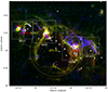 |
Fig. 1. RGB image (red: Herschel-PACS at 250 μm, green: MSX at 8.28 μm, blue: PMO 13CO(1–0) in the integrated local standard of rest velocity range from –63 to –28 km s−1) of the W5 star-forming complex. The 250 μm emission is dominated by warm dust heated by absorbed starlight. The interface between the ionized and molecular gas appears as a blend of green (strong 8 μm emission from PAHs), and blue (representing the colder CO molecular gas). The entire area displayed by the figure has been mapped in three CO J = 1–0 isotopologues (see Sect. 3.1). The red boxes represent the areas in which NH3 has been observed. The two yellow dotted circles represent the boundaries of the two bubbles, W5-E and W5-W. The definition of the boundary was taken from a catalog of HII regions (Anderson et al. 2014) based on all-sky Wide-Field Infrared Survey Explorer (WISE) data. Four white dotted boxes mark the extent of the four areas studied in this article (W5-E1, W5-M, W5-W1, and W5-W2). White stars and black plus signs indicate identified OB stars (Roman-Lopes et al. 2019) and high-mass young stellar objects (HMYSOs) (Lumsden et al. 2013), respectively. Due to the specific location of W5, the galactic longitude and latitude axes are to first order roughly parallel to right ascension and declination (RA and Dec). |
Considering the identification of OB stars in the W3-W4-W5 region (Roman-Lopes et al. 2019), it is evident that W5-E harbors three OB stars, while W5-W contains seven OB stars. Notably, Karr & Martin (2003) calculated that the OB stars within W5-W generate an excess of ionizing photons beyond what is necessary for ionizing the HII regions, indicating that the region is not entirely ionization-bound. This finding gains further support when considering that their calculations referred to only four OB stars. Additional support for the notion of a triggered star-forming region in W5-E was provided by Niwa et al. (2009), who employed CO data from the 45-m telescope at the Nobeyama Radio Observatory. Moreover, Deharveng et al. (2012) employed Herschel observations to identify young stellar objects (YSOs) throughout the W5 complex. Through a classification based on the evolutionary stage, it was revealed that star-forming activity was triggered primarily at the boundary of the HII regions. Insightful contributions to our understanding by the Purple Mountain Observatory (PMO) CO molecular gas within 110 deg2 in the W3-W4-W5 region were provided by Sun et al. (2020). Furthermore, Li et al. (2019, 2020a) utilized CO data to detect outflows within the same region and meticulously analyzed the ensuing feedback effects onto the surrounding molecular clouds.
Overall, CO and its isotopologues stand out as crucial indicators of molecular clouds (Dame et al. 2001). This tracer reveals the distribution of the molecular gas as well as essential information on the kinematics (e.g. Shu et al. 1987). Generally, 12CO is optically thick (e.g. Goldsmith & Langer 1999), whereas 13CO and C18O offer greater optical thinness (Hacar et al. 2016), rendering them ideal for tracing relatively dense regions. Numerous researchers have harnessed CO gas as a valuable tool for meticulously scrutinizing the intricate morphological and dynamical aspects of molecular clouds, as well as the star-forming activity within clumps. Notably, a high-resolution C18O emission map with exceptional angular and velocity precision provided an initial overview of the filamentary structure within the Orion A molecular cloud (Suri et al. 2019). Additionally, Goodman et al. (2009a) and Mazumdar et al. (2021a) employed clumps identified using 13CO to analyze their evolutionary properties. Furthermore, the identification of clump structures was accomplished through millimeter observations of C18O, as highlighted by Takekoshi et al. (2019) and Lin et al. (2021).
Far-ultraviolet (FUV) radiation emanating from massive stars exerts a profound influence on the structural, chemical, and thermal characteristics of the ambient medium (Hollenbach & Tielens 1997). Regions predominantly steering the energetic and chemical equilibrium of these gaseous environments are denoted as photon-dominated regions (PDRs) (Tielens & Hollenbach 1985; Hollenbach et al. 1991; Shimajiri et al. 2014). Within PDRs, C18O exhibits heightened susceptibility to FUV radiation-induced effects in comparison to 13CO, potentially leading to isotope selective photodissociation (Minchin et al. 1995; Kong et al. 2015; Yamagishi et al. 2019).
Concurrently, due to different degrees of self-shielding, the spatial extent of the gas giving rise to C18O emission may be diminished with respect to the more abundant isotopologues (Glassgold et al. 1985; Yurimoto & Kuramoto 2004; Liszt 2007; Röllig & Ossenkopf 2013). Furthermore, the study on cloud clumpiness by Zielinsky et al. (2000) reveals an augmentation in the dissociation rate with diminishing column density, attributable to self-shielding effects. Thus, it is evident that 13CO/C18O represents a powerful tool to scrutinize the impact of FUV photon irradiation onto the molecular gas (Areal et al. 2019).
A highly valuable instrument for identifying regions affected by stellar feedback is MSX, at 8.28 μm. It serves as a tracer of polycyclic aromatic hydrocarbons (PAHs) whose emissions are stimulated by far-ultraviolet (FUV) photons originating from stars within the central cavity. Mazumdar et al. (2021a,b) successfully delineated the feedback region in the G305 giant molecular cloud complex using the GLIMPSE 8 μm flux, subsequently analyzing the impact of feedback from OB stars on the distribution of molecular clouds and the evolutionary trajectory of clumps. Furthermore, Li et al. (2020a) meticulously explored the repercussions of feedback from CO outflow candidates on their parent clouds, examining an extensive area of 110 deg2 encompassing the W3-W4-W5 complex and its surroundings.
In this paper, we mainly use the three CO isotopologues in their ground rotational transition to analyze the overall structural distribution of clouds and combine them with NH3 molecular line data to analyze the physical properties of the specific clumps. The paper is organized as follows. In Sect. 2, we introduce our observations and data reduction. The overall distributions of CO and NH3 as well as kinetic temperatures and column densities of the individual clouds are highlighted in Sect. 3, complemented with an analysis of potential CO-depletion in their densest parts. In Sect. 4, we identify the clump structure from the 13CO emission using Dendrogram and calculate the parameters for each clump. In Sect. 5, we analyze the feedback effect of the two H II regions of W5 on the surrounding molecular gas and the evolutionary state of the clumps, as well as the effect of outflowing gas within the molecular cloud on clumps. Our main conclusions are summarized in Sect. 6.
2. Observations and data reduction
2.1. CO(1–0) molecular line data for whole W5
We mapped a 2.75° × 2.4° region centered at l = 137.375°, b = 1.2° of the W5 molecular clouds (6.6 deg2, part of the 110 deg2 data of Sun et al. 2020 and Li et al. 2019, 2020a) making use of the Milky Way Imaging Scroll Painting (MWISP) project. This is a multi-line survey in 12CO/13CO/C18O (J = 1–0) along the northern galactic plane carried out by the Purple Mountain Observatory (PMO) 13.7 m telescope. The MWISP project led by the PMO is a large ongoing project whose goal is to map CO and its isotopic transitions covering the accessible part of the Galactic plane (Su et al. 2019). Using a nine-beam superconducting spectroscopic array receiver, working in the sideband separation mode and employing a fast Fourier transform spectrometer (Shan et al. 2012), the three CO isotopologues (12CO, 13CO, and C18O) were observed simultaneously.
The 12CO line was observed in the upper sideband with a half-power beamwidth (HBPW) of 49″. The 13CO and C18O lines were observed in the lower sideband with a half-power beamwidth (HPBW) of 51″, and the data were gridded to 30″ pixels for all three transitions. Both bandwidths were 1000 MHz with 16 384 channels, resulting in velocity separations of about 0.16 km s−1 for 12CO and 0.17 km s−1 for 13CO and C18O. The typical system temperature was 280 K for 12CO and 185 K for 13CO and C18O. The pointing accuracy of the telescope was better than 5″. Mapping observations used the on-the-fly (OTF) mode with a scan speed of 50″ s−1 and a step between consecutive scans of 15″, yielding an integration time of 14 seconds per position. The final data are recorded on a main beam brightness temperature scale (Tmb) and were reduced using Astropy1. Please also refer to Xu et al. (2006), Sun et al. (2020) and Li et al. (2019, 2020a) for a more detailed description of the observations and data-reduction strategies.
2.2. NH3 data in the four densest regions
We used the Xinjiang Nanshan 26-meter radio telescope to observe the NH3(1,1) and NH3(2,2) lines in the K-band towards four compact regions located in the W5 molecular cloud, covering a total of 0.1 square degrees. The four observed areas are marked with red boxes in Fig. 1. The rest frequency was set to 23.708564 GHz to observe simultaneously the NH3 (1,1) and (2,2) lines at 23.694495 and 23.722633 GHz. At this frequency, the telescope’s main beam full width at half maximum (FWHM) is ∼125″ and the velocity resolution is ∼0.1 km s−1 achieved with an 8192-channel digital filter with a bandwidth of 64 MHz. The antenna temperature  has been converted to main beam brightness temperature, Tmb, using a beam efficiency of 0.59. The typical system temperature was 50 K (
 scale) at 23.708 GHz. The telescope pointing and tracking accuracy is better than 18″. The maps were made using the on-the-fly (OTF) mode with 6′×6′ grid size and 30″ sample step. All observations were obtained under excellent weather conditions and above an elevation of 20°. The Tmb scale has an estimated calibration uncertainty of about 14% (Wu et al. 2018). The CLASS and GREG packages of GILDAS2 were used for the NH3 data calibration and fitting. The final data cube has a pixel size of 30″ and the velocity resolution has been smoothed to 0.3 km s−1.
3. Integrated properties of molecular clouds
3.1. CO distribution
As mentioned in Sect. 1, we present an RGB plot of the W5 region in Fig. 1, indicating that the molecular gas distribution is associated with two large bubbles in this proximity: W5-W and W5-E. The distribution of hot dust and PAHs coincides with the distribution of the two bubbles, while cold molecular gas is almost entirely distributed in the shells of the two bubbles.
To create the integrated intensity (“moment-0”) maps of the W5 region, a noise map of each grid element (referred to as a pixel) was created for the 12CO, 13CO, and C18O J = 1–0 transitions. To reduce the influence of noise, the 12CO, 13CO, and C18O data were integrated over all channels which had at least three contiguous channels above the 3σ level. Fig. 2 shows our moment 0 maps of the W5 star-forming complex. The 12CO map traces the diffuse large scale molecular structures as well as the cold gas. The 13CO map is sensitive to higher column density gas and hence, traces the more compact, dense clumps in the complex. C18O emission on the other hand only appears in the densest parts, generally corresponding to the filament and core structure. The 12CO gas is mainly distributed in the diffuse shells at the W5-E and W5-W boundaries, corresponding to W5-W1, W5-W2, W5-E1, and W5-M in Fig. 1. Then, 13CO shows the same trend, but only in the dense areas. On the other hand, C18O exhibits a completely different distribution; namely, W5-M appears to be almost devoid of C18O, while emission is mainly present in W5-W2 and W5-E1.
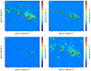 |
Fig. 2. Moment 0 maps of three CO isotopologues in the W5 region. The integrated local standard of rest velocity range is from VLSR = –50 to –30 km s−1. The first three figures are 12CO, 13CO, and C18O moment 0 maps of integrated intensity. The last one is a comparison of the three isotopologues superimposed, where the background color is the 12CO intensity, the contour line is the 13CO intensity, and the grey areas refer to positions with notable C18O emission. The yellow stars, black crosses, and small green and red dots in each map mark OB stars, HMYSOs (Lumsden et al. 2013), and blue and red lobes identified as CO outflows by Li et al. (2019), respectively. |
The averaged spectra of 12CO (black), 13CO (blue), and C18O (red) for the whole W5 region are shown in Fig. 3. It can be seen from the figure that the distribution of the average spectral line does not conform to a Gaussian distribution, and there is an additional velocity component in the spectral profile, which is 2.9 km s−1 off the main velocity component. All the emission from the complex is found within the velocity range from –47 to –32.5 km s−1 for 12CO, and –42.5 to –34 km s−1 for 13CO. Fig. 4 shows the three CO emission velocity channel maps (from top to bottom: 12CO, 13CO and C18O) of the W5 complex in the local standard of rest velocity range from –50 to –30 km s−1 with a spacing of 3.3 km s−1. It is evident that the radiation of the three dense regions W5-E1, W5-M, and W5-W1 located at the boundary of W5-E and W5-W are mainly distributed between –43 and –36.6 km s−1, while W5-W2 emission is mainly distributed between –36 and –33.3 km s−1. The observed velocity structure is most likely a consequence of the interplay of the morphology of the cloud and the feedback from the central star clusters on the natal molecular cloud (see Sect. 5.1).
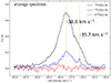 |
Fig. 3. Average spectrum of 12CO (black), 13CO (blue), and C18O (red) in the entire mapped area (see Fig. 1) containing the W5 region. |
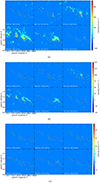 |
Fig. 4. Velocity channel maps of 12CO(1–0) (a), 13CO(1–0) (b) and C18O(1–0) (c) toward W5. The emission has been integrated over 3.3 km s−1 around the local standard of rest velocities indicated in each panel. Note: the intensity of each detected and displayed pixel is greater than 3σ. For the yellow stars and small green and red dots, see Fig. 2. |
3.2. NH3 distribution
The CO results in Sect. 3.1 indicate that the densest regions within W5 (W5-W1, W5-M1, AFGL-4029, and sh-201) are situated along the shell layers at the boundary of the W5 HII regions. 12CO, 13CO, and C18O (1–0) can serve as column density tracers (Dame et al. 2001), but are susceptible to selective photodissociation effects (Minchin et al. 1995; Kong et al. 2015; Yamagishi et al. 2019).
Complementing CO, NH3 is highly affected by UV irradiation but is able to survive in well shielded pockets with sufficiently high H2 column density (e.g. Mühle et al. 2007; Ott et al. 2010). NH3 experiences less freeze out onto dust grains, particulary in the high-density environments of dense cores (Townes et al. 1983; Walmsley & Ungerechts 1983; Danby et al. 1988; Henkel et al. 2012) and is also crucial for determining the kinetic temperature of the denser gas in the bubble-shell clouds. To gain a comprehensive understanding of the molecular gas nature, a comparison between CO isotopologues and NH3 emission is thus indispensable.
To obtain the gas distribution and kinetic temperature of the dense regions in the W5 molecular cloud complex, we present the NH3 (J, K) = (1,1) and (2,2) intensity maps in the four densest regions sh-201, AFGL 4029, W5-M1, and W5-W1 (from east to west) in Fig. 5. The results show that AFGL 4029 has the strongest signal in the two NH3 lines, while W5-M1 and W5-W1 show almost no signal. Figure 6 illustrates the NH3 spectrum in AFGL 4029. The optical depth of the NH3 (1,1) line was determined using the fitting method in the GILDAS software, yielding a value of 0.1 ± 0.013. There are a total of 5 HMYSOs in the three subregions, W5-W1, W5-M1, and AFGL 4029, represented by black stars in Fig. 5. Almost every HMYSO is associated with an NH3(1,1) clump, except in the W5-m1 region, which also exhibits little C18O emission. The distribution of HMYSOs shows that almost all of these YSOs are located at the inner side of the rim of the bubble. This may be due to the continuous action of the central stellar wind that causes more molecular gas to accumulate at the edges of W5-E and W5-W, allowing stars to form earlier here than in other regions. The NH3 signal is weak and optically thin throughout the region. Although many authors have shown that the two HII regions in the W5 region have an obvious feedback effects on the surrounding environment and trigger the formation of surrounding stars (e.g., Niwa et al. 2009; Deharveng et al. 2012), it is difficult to determine the detailed evolutionary stages of individual HMYSOs.
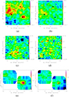 |
Fig. 5. Intensity maps of NH3 (J, K) = (1,1) and (2,2) lines for W5-W1, W5-M1, AFGL 4029 and sh-201, respectively. The LSR velocity intervals of the integration are –45 to –32 km s−1 (W5-W1), –40 to –36 km s−1 (W5-M1), and –42 to –36 km s−1 (AFGL 4029 and sh-201), respectively. Contours of integrated intensity start at 0.09 (W5-W1), 0.07 (W5-M1), and 0.08 (AFGL 4029 and sh-201) K km s−1 (3σ) on a main beam brightness temperature scale and go up in steps of 0.03 (W5-W1), 0.01 (W5-M1), and 0.05 (AFGL 4029 and sh-201) K km s−1. The black stars represent HMYSOs identified by Lumsden et al. (2013). (a) W5-W1: NH3(1,1), (b) W5-W1: NH3(2,2), (c) W5-M1: NH3(1,1), (d) W5-M1: NH3(2,2), (e) AFGL4029, sh-201: NH3(1,1), (f) AFGL4029, sh-201: NH3(2,2). |
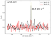 |
Fig. 6. Spectra of NH3 (1,1) (black) and NH3 (2,2) (red) in the dense core AFGL 4029 (see Fig. 1). The yellow dotted line marks the position of the LSR-velocity at the centroid of the (1,1) line. |
To exclude the positions with a low level of emission, we performed a signal-to-noise ratio (S/N) screening for NH3 (1,1) and (2,2). The criterion is that the strongest signal channel of each spectral line and the adjacent two channels must meet > 3σ. Since the NH3(2,2) line signal is weak, and the NH3(1,1) signal of W5-M1 is also weak, only the velocity and dispersion distributions of NH3(1,1) lines stronger than 3σ in the AFGL 4029, sh-201 and W5-W1 regions are given in Fig. 7. It turns out that the three dense clumps in W5-W1 show completely different velocities, with differences up to 6.7 km s−1 with respect to the other clumps, and the same trend is obtained for the CO emission. The largest clump in W5-W1 (located on the eastern side of W5-W1 in Fig. 5(a), MCO(clump) ≈ 4.3 × 10⁴ M⊙ calculated using Eq. (14); see below) exhibits a velocity distribution ranging from –41.5 to –38.5 km s−1. The clump positioned in the northwest at high latitude of the figure displays a velocity distribution between –43 to –42 km s−1, while the clump in the southwest at lower latitude shows a velocity distribution ranging from –36.5 to –35 km s−1. Concurrently, the velocity dispersion reveals notably higher values at higher latitudes of the largest clump. These observations collectively underscore the dynamical nature of the W5-W1 region, indicative of intense stellar formation activity.
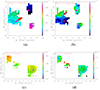 |
Fig. 7. NH3(1,1) line velocity and dispersion distributions in W5-W1, AFGL 4029 and sh-201. Contours are integrated intensity and red stars mark the HMYSOs. Only the pixels with integrated intensities larger than 3σ are presented. (a) W5-W1: velocity, (b) W5-W1: dispersion, (c) AFGL4029, sh-201: velocity, (d) AFGL4029, sh-201: dispersion. |
3.3. The gas kinetic temperature
Assuming local thermal equilibrium (LTE) (Wilson et al. 2009; Shirley 2015), we use the 13CO J = 1–0 emission to determine the column density and molecular mass of the W5 region assuming that the 12CO emission is optically thick. To test the applicability of the optically thick assumption for 12CO, we use the method for correcting optical depth effects by Henkel et al. (1980, 1982, 1983, 1985) to calculate the 12CO/13CO integrated intensity ratio for all pixels where both 12CO and 13CO signals are above 3σ. The median and mean values are found to be 6.3 and 7.9, respectively; these values are significantly lower than the carbon isotope ratio obtained by Yan et al. (2023) for W3(OH) ([12C/13C] = 75 ± 4, deduced from optically thin CS isotopologues observed with the IRAM (Institut de Radioastronomie Millimétrique) 30 m telescope). This clearly indicates that 12CO is optically thick. Furthermore, the ratio between [12C/13C] and the measured ICO/I13CO line intensity ratio suggests characteristic 12CO line opacities of order 10. Because of [12C/13C] ≫ 10, this also infers that 13CO should be optically thin towards most positions. With hν/k = 5.53 K (h: Planck constant; k: Boltzmann constant) for the CO J = 1–0 line, TCMB = 2.73 K for the cosmic background radiation and a beam filling factor of unity, we obtain with the equation of radiative transfer the line temperature Tmb in units of Kelvin,
![Mathematical equation: $$ \begin{aligned} T_{\rm mb} = 5.53 [e^{-5.53/T_{\rm ex}} - e^{-5.53/2.73}]^{-1}. \end{aligned} $$](/articles/aa/full_html/2024/09/aa47972-23/aa47972-23-eq3.gif) (1)
(1)
Here, Tex is the only unknown quantity. Main beam brightness temperatures of the 12CO line peaks indicate that Tex, for the entire W5 region depicted in Fig. 8(a) (this includes regions not detected in 13CO, where even 12CO may be optical thin or subthermal), ranges from 3.3 to 35.3 K with an average of 11.9 ± 4.5 K.
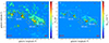 |
Fig. 8. Maps of (a) CO excitation temperature distributions and (b) H2 column density distribution traced by 13CO. The gray dotted boxes mark the four dense regions (W5-E1, W5-M, W5-W1, and W5-W2 described in Fig. 1). |
The critical density of the 12CO J = 1–0 line in the optically thin limit, when collisional de-excitation matches spontaneous decay, is ∼103.5 cm−3 (e.g. Mao et al. 2000). Because the line is saturated with the above mentioned opacity of about 10, the effective critical density is even lower by approximately a full order of magnitude. For gas with densities in excess of 103 cm−3, that is required for environments with detected ammonia emission (e.g. Ho & Townes 1983), the excitation temperature is thus a good estimate of the kinetic temperature.
Due to the limitations of CO with respect to the observations of dense areas, this analysis should be complemented by NH3. The relative populations of the K = 1 and 2 ladders of ammonia are dominated by collisional processes. Therefore we can also use NH3 as a thermometer of the gas kinetic temperature for the denser region where not only the (1,1) but also the (2,2) line is visible with sufficent S/N. Due to the weak NH3 signal in W5-M1 (in W5-M), we detected the (2,2) line signal only at two locations, towards the clumps W5-W1 (in W5-W) and AFGL 4029 (in W5-E).
Following Townes et al. (1983), the rotation temperature of NH3(1,1) and (2,2) is obtained by:
![Mathematical equation: $$ \begin{aligned} T_{\rm rot} = \frac{-41.5}{ln[\frac{-0.282}{\tau _m(1,1)}ln[1-\frac{T_{\rm MB}(2,2)}{T_{\rm MB}(1,1)}[1-exp(-\tau _m(1,1))]]]} \, \mathrm{K}, \end{aligned} $$](/articles/aa/full_html/2024/09/aa47972-23/aa47972-23-eq4.gif) (2)
(2)
where τm is the peak optical depth of the (1,1) main group of hyperfine components derived using the GILDAS built-in “NH3(1,1)” fitting method. The main beam brightness temperatures Tmb of the (1,1) and (2,2) inversion transitions are derived using the GILDAS built-in “GAUSS” fitting. We can then calculate Tkin, based on Trot (Tafalla et al. 2004):
 (3)
(3)
Qualitatively, both NH3 and CO exhibit their strongest signals in several dense cores at the boundary of the HII regions. Nevertheless, there may be small discrepancies in temperatures of AFGL 4029 and W5-W1, the only two clumps that were detected in NH3 (2,2). For W5-W1, Tkin drived from NH3 ranges from 9.7 to 21.6 K with an average of 14.0 ± 3.6 K in W5-W1, while Tex drived from 12CO ranges from 18.7 to 22.5 K with an average of 20.7 ± 1.0 K. For AFGL 4029, Tkin values range from 8.3 to 9.9 K with an average of 9.0 ± 0.4 K, while Tex ranges from 18.8 to 35.3 K with an average of 27.6 ± 4.3 K. It is clear that the Tex values from CO are higher than the Tkin values from NH3 in the clump of AFGL 4029, while there are small discrepancies in W5-W1. The temperature discrepancy in the former source may arise from Tex being calculated from optically thick 12CO, potentially tracing more diffuse gas in the outskirts of the clumps, while NH3 traces the denser regions. While the resolution of NH3 is limited, and the signal-to-noise ratio is relatively low, potentially introducing some uncertainties in the results. The discrepancy in AFGL 4029 is clearly large enough to be significant.
3.4. Column densities
The LTE assumption is a crucial factor determining 13CO column densities. In the non-LTE case, the excitation temperature of the 13CO (1–0) lines may be very different from that of 12CO (1–0) (Liu et al. 2012). We applied RADEX3 (van der Tak et al. 2007) to investigate the effect of non-LTE conditions on the determination of the column density of 13CO. The median value of the 13CO column density under the LTE assumption is 2.0 × 1015 cm−2. The median value of the 12CO and 13CO line widths are 1.5 km s−1 and 0.5 km s−1. For Tkin = 15 K and an H2 volume density of 103 to 104 cm−3, we simulated the emission of 12CO (1–0) and 13CO (1–0) in a parameter space for Tex of 8.3–16.1 K using RADEX. The simulated Tex value is not much different from the initial Tkin, so the LTE assumption is applicable for those pixels where both 12CO and 13CO were detected.
We used TMB, 12 and TMB, 13 for the main-beam brightness temperature of 12CO and 13CO, respectively. All the voxels satisfy the conditions TMB, 12 > TMB, 13; we further assume that the excitation temperature of 13CO is equal to the excitation temperature of 12CO in the voxels both 12CO and 12CO are detected. The optical depth of 13CO(τ13) under LTE assumption is estimated as (Kawamura & Masson 1998; Pineda et al. 2010)
![Mathematical equation: $$ \begin{aligned} \tau _{13} = -ln[1-\frac{T_{\rm MB,13}}{5.29}[(e^{5.29/T_{\rm ex}}-1)^{-1}-0.164]^{-1}], \end{aligned} $$](/articles/aa/full_html/2024/09/aa47972-23/aa47972-23-eq6.gif) (4)
(4)
where TMB, 13 is the peak main beam brightness temperatures of 13CO. I13 is a function of the total integrated intensity of 13CO. It can be estimated from 13CO(τ13):
 (5)
(5)
Finally, the column densities of 13CO can be estimated by the following equation (Garden et al. 1991):
 (6)
(6)
Fig. 8(b) shows the H2 column densities that were derived using a carbon isotope ratio of [12C/13C] = 75.3 (Wilson & Rood 1994; Henkel et al. 1994; Yan et al. 2019, 2023) for a W3(OH) galactocentric distance of 9.64 kpc, and an [H2/12CO] abundance ratio of 1.1 × 10⁴ (Frerking et al. 1982). For a given cloud, the 12C/13C isotope ratio from H2CO gives an upper limit and the ratio from CO provides a lower limit to the actual ratio (Langer et al. 1984; Tang et al. 2019).
According to Mauersberger et al. (1986) the NH3 column density in the J = 1, K = 1 state related to the optical depth τtot, is:
 (7)
(7)
where N is in cm−2, the FWHM line width Δv is in km s−1, the line frequency ν is in GHz, and the excitation temperature Tex is in Kelvin. The excitation temperature Tex is determined by both the main beam brightness temperature Tmb and the optical depth τ,
 (8)
(8)
Then the total ortho- plus para-NH3 column densities can be calculated from NH3(1,1). Following Wienen et al. (2012) and Tursun et al. (2020), we obtain
 (9)
(9)
assuming that the bulk of the NH3 population resides in the metastable (J, K) = (0,0) to (3,3) inversion levels. The total-NH3 column densities (Ntot) range from 0.68 × 10¹⁴ to 1.58 × 1014 cm−2 with an average of 1.1 ± 0.21 × 1014 cm−2 in W5-W1. In AFGL 4029 the total-NH3 column densities become 1.13 × 10¹⁴ to 3.85 × 1014 cm−2 with an average of 2.52 ± 0.52 × 1014 cm−2. In contrast to the kinetic temperature distribution (Sect. 3.3), W5-W1 has lower column densities, while AFGL 4029 has higher column densities. The column density difference may be caused by the fact that the bubble diameter of W5-E with sh-201 and AFGL 4029 is smaller than that of W5-W. Therefore the time of the molecular gas surrounding W5-E being affected by the HII regions may be shorter (the ages of the HII regions W5-E and W5-W are between 1.7 and 3.0 Myr and between 2.4 and 5.0 Myr (the latter 5 Myr, if the most massive O stars formed last), respectively Karr & Martin (2003). Although the expansion of the bubble accelerated star formation activity in the surrounding molecular cloud, as the circumference continues to grow, it will easily diffuse the molecular gas into a larger space, thereby reducing the density of the molecular gas.
3.5. NH3 (1,1) versus C18O (1–0) emission
In this subsection, we compare the intensity distributions of the optically thin lines of NH3(1,1) and C18O (1–0) in the molecular clouds and their implications for our understanding of the molecular depletion process. The depletion of molecular species onto dust grains is a fundamental process in molecular clouds, and NH3(1,1) and C18O are commonly used as tracers of dense gas in these regions. As noted by Tafalla et al. (2002), C18O is expected to be more significantly depleted than NH3(1,1) due to its higher binding energy to dust grains. This may lead to differences in the intensity distribution of these molecules, particularly in cold, dense molecular cores where the depletion is most significant. By comparing the intensity distributions of NH3(1,1) and C18O, we can gain insight into the physical conditions and depletion processes in dense molecular clouds.
Fig. 9 shows us the NH3(1,1) and C18O intensity distribution in the W5-W1 and AFGL 4029 regions, and it is clear that the morphological distributions of NH3 and C18O are almost indistinguishable except for a clear separation in a clump to the north (higher galactic latitude) of sh-201. To further analyse the relationship between the two molecules, we reduced the resolution of C18O to that of NH3(1,1), so that we could analyse the relationship pixel by pixel. Fig. 10 shows this distribution. We can clearly see that individual sources show a linear correlation, while these linear correlation in W5-W1 and AFGL 4029 show significantly different trends. In this context it may be relevant (see also Sects. 3.3 and 3.4) that W5-W1 has a higher Tkin, NH3 value (9.8–18.2 K with an average of 13.2 ± 1.7 K) and lower column density Ntot, NH3 (0.68 × 10¹⁴ to 1.58 × 1014 cm−2 with an average of 1.1 ± 0.21 × 1014 cm−2), while AFGL 4029 has a higher column density Ntot, NH3 (1.13 × 10¹⁴ to 3.85 × 1014 cm−2 with an average of 2.52 ± 0.52 × 1014 cm−2) and a lower Tkin, NH3 value (8.3–10 K with an average of 9.2 ± 0.6 K). For W5-W1, the lower column density discerned within the region exhibiting the heightened C18O/NH3 intensity ratio could contribute to reduced shielding effects against external radiation. This diminishment in shielding potential might foster more efficient heating and subsequent sublimation of CO molecules from the surfaces of dust grains.
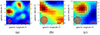 |
Fig. 9. Color map of the velocity integrated intensities (moment 0) for the C18O line in the regions W5-W1, sh-201 and AFGL 4029. The white and black contours denote the intensity of C18O and NH3(1,1), respectively. The red circles in the lower left and red lines in the lower right of each panel mark the NH3(1,1) beam size (120″) and 0.5 pc length, respectively. (a) W5-W1, (b) sh-201, (c) AFGL4029. |
 |
Fig. 10. The point-to-point intensity distribution of NH3(1,1) and C18O in the three regions of Fig. 9. The red, blue, and green dots correspond to the areas W5-W1, AFGL 4029, and sh-201, respectively. The red, blue, and green lines are linear fits to the three types of scatters. |
4. Clumps identified in the 13CO emission line
4.1. Extracting clumps: Dendrogram
A dendrogram can be interpreted as a tree that represents the hierarchy of the structures in data and decomposes the intensity data cube into a nested hierarchy of structures called trunks, branches, and leaves. Branches split up into multiple sub-structures, namely, leaves with no discernible sub-structure. Trunks can split up into branches and leaves, which allows hierarchical structures to be adequately represented. The term trunk is used to refer to a morphological feature that has no parent structure.
The astrodendro4 package was run on the data cube in position-position-velocity (PPV) space. The dendrogram algorithm has three input parameters (min_value, min_delta, and min_pix). The min_value was set to 3 × rms to avoid getting structures with peak intensity below the noise threshold. The rms values are the rms noise levels measured in a region of the integrated intensity map where no line emission was detected. With min_delta = 3 × rms, a structure was considered independent only if its peak brightness differed by at least 3 × rms from the nearest local maximum. min_npix = 18 pixels (pixel size = 30″), the minimum number of pixels a structure must contain to remain independent. This parameter prevents noise spikes from being identified as sources. The distribution of identified leaves is shown in Fig. 11, with a total of 212 leave structures.
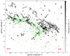 |
Fig. 11. Identified clumps (leaves) in 13CO cube data. Clumps are marked by a black contour line in the figure. The grey intensity map is a moment 0 map of 13CO in the LSR-velocity range –50 to –30 km s−1. The red and green dots represent the class I and class II Young Stellar Objects (YSOs) classified by Koenig et al. (2008). |
4.2. Catalog of clump properties
After running the dendrogram algorithm on the data cube, a catalog of properties of all the structures can be created. We extracted the leaves’ morphology from these distributions and treated the leaves as clump structures that could lead to new star formation. The catalog gives information such as the location, mean velocity, total fluxes within the structure, and radius of each leaf on the position-position plane (Rosolowsky & Leroy 2006). Other parameters such as luminosity, virial parameter and thermal velocity dispersion of the clumps are calculated according to the following equations (Eqs. (10)–(18)). All properties of the 212 clumps of 13CO (see Fig. 11) are summarized in Table 1.
Part of the clump properties derived from 13CO dendrogram leaves of W5.
The radius from the algorithm catalog is in arcsec. We use Rpc = Rarcsecd to calculate the physical radius in pc and L = Fd2 to calculate their luminosities, where d = 1.95 ± 0.04 × 10³ pc is the distance to W3(OH) (Xu et al. 2006), F has units of K km s−1 arcsec2, and L has units of K km s−1 pc2. Rpc, flux and the luminosity of the cloud, LCO (Rosolowsky & Leroy 2006) can be defined as:
![Mathematical equation: $$ \begin{aligned} R[\mathrm{pc}]&= \frac{\mathrm{R}[\mathrm{arcseconds}]}{3600}\frac{\pi }{180}{d}[\mathrm{pc}]\end{aligned} $$](/articles/aa/full_html/2024/09/aa47972-23/aa47972-23-eq12.gif) (10)
(10)
 (11)
(11)
![Mathematical equation: $$ \begin{aligned} L_{\rm CO}[\mathrm{K\,km\,s}^{-1}\,\mathrm{pc}^2]&= \nonumber \\&F_{\rm CO}[\mathrm{K\,km\,s}^{-1}\,\mathrm{arcsec}^2]({d}[\mathrm{pc}])^2\left(\frac{\pi }{180\times 3600}\right)^2 \end{aligned} $$](/articles/aa/full_html/2024/09/aa47972-23/aa47972-23-eq14.gif) (12)
(12)
If δx and δy are in units of arcseconds, δv in km s−1, and Ti in K, then the resulting flux will have units of K km s−1 arcsec2.
The velocity dispersion σv can be defined from the FWHM of ΔV
 (13)
(13)
The mass of each clump can be determined by summing up the masses of all the pixels within each leaf. The mass for each pixel is computed as:
![Mathematical equation: $$ \begin{aligned} M_{\rm pixel} = N_{\rm tot}(^{13}\mathrm{CO})[\mathrm{H}_2/\mathrm{C}^{13}\mathrm{O}]\mu _{\rm H_2}m_{\rm H} A_{\rm pixel}, \end{aligned} $$](/articles/aa/full_html/2024/09/aa47972-23/aa47972-23-eq16.gif) (14)
(14)
where μH2 = 2.72 is the mean molecular weight (Brunt 2010), mH = 1.67 × 10⁻²⁴ g is the mass of a hydrogen atom, [H2/13CO] is assumed to be 8.3 × 10⁵ (from isotope ratios in Sect. 3.4), and Apixel is the area of each pixel within the clump.
The volume density and surface mass density of clumps can be given using their mass and radius:
 (15)
(15)
and
 (16)
(16)
Here, M is in M⊙, Rpc is in pc, n(H2) is in cm−3, and ∑ is in g cm−2. The factor of 15.1 is used to convert the density to appropriate units.
To estimate the virial stability of these clumps, we adopt the virial analysis method described in Mazumdar et al. (2021b). The virial parameter is defined as the ratio of the virial mass of a spherically symmetric cloud to its total mass:
 (17)
(17)
where σv is the velocity dispersion of the clump and G is the gravitational constant (MacLaren et al. 1988). We assume that these clumps follow a spherical density distribution. In the absence of pressure supporting the clump, αvir < 1 means that the clump is gravitationally unstable and collapsing, whereas αvir > 2 suggests that the kinetic energy is higher than the gravitational energy and that the clump is dissipating. A value of αvir between 1 and 2 is interpreted as an approximate equilibrium between the gravitational and kinetic energies.
The luminosity-to-mass ratio (L/M) of clumps is a good indicator of their evolutionary stage in star formation (Molinari et al. 2008; Urquhart et al. 2018).
To determine the dominant broadening mechanisms, we calculate thermal line widths using  in units of km s−1, where k is the Boltzmann constant in units of J/K, m is the mean molecular mass in units of g, and T is the excitation temperature, Tex, from Eq. (1). The thermal and non-thermal line widths (σThermal and σNon − Thermal) are defined using the following equations (Myers 1983; Li et al. 2015):
 (18)
(18)
and
 (19)
(19)
where σ1D is the one-dimensional velocity dispersion in units of km s−1, △v13 is the line width in units of km s−1, k is the Boltzmann constant in units of J/K, μ = 2.4, mH is the mass of a single hydrogen atom in units of g and T is the excitation temperature in units of K.
5. Impact of feedback on molecular gas and clumps
Since W5 contains two large bubbles of different diameters surrounding different numbers of OB stars, the radiation and ionization fronts from the OB stars in the central cavity also have different effects on their surrounding molecular clouds. Typically, this effect is manifested by the injection of turbulent kinetic energy into the surrounding molecular cloud, which compresses the gas or makes it unstable against gravitational collapse at the inner sides of the outer boundaries of the bubbles. Our distributions of Tex and column densities of 13CO, as well as the results of Niwa et al. (2009) and Deharveng et al. (2012) indicate that the W5 molecular cloud is affected by this process. In the following, we will mainly use the distribution of molecular line intensities and clump properties to analyze the effect of the supersonic expansion of the HII regions on the surrounding molecular gas and its relation to star formation activity.
5.1. Effects of feedback on the molecular gas
5.1.1. 13CO/C18O abundance ratio
Maps of the excitation temperature and H2 column density are presented in Fig. 8. The regions with higher excitation temperatures in both W5-E and W5-W are all located at the inner rims of the bubbles, while almost all other regions have lower excitation temperatures Tex < 10 K. The elevated excitation temperatures observed in the former regions may serve as direct evidence of the molecular gas at the boundaries of the HII regions being influenced by the radiations from the central OB star clusters, W5-E and W5-W. This assertion finds support in the research conducted by Niwa et al. (2009) and Deharveng et al. (2012) on W5. Concurrently, the residual portion of the surveyed molecular gas is situated within regions characterized by lower excitation conditions (Goldsmith et al. 2008; Pineda et al. 2008).
Since C18O with its lower opacity may be more efficiently dissociated by far-ultraviolet (FUV) photons than 13CO (Shimajiri et al. 2014), abundance variations of these isotopologues across different environments can be used as an indicator of the evolutionary stages of molecular clouds (van Dishoeck & Black 1988; Shimajiri et al. 2014). According to the relation between X(13CO)/X(C18O) and N(13CO), Wang et al. (2019) defined two types of molecular clouds (MCs). Type I MCs have lower abundance ratios X(13CO)/X(C18O), lower 13CO column densities and lower excitation temperatures. Type II clouds show the opposite behavior. Hence, type I molecular clouds are likely to be either quiescent clouds or in the early stages of star formation. In contrast, type II molecular clouds encompass active star-forming regions and are markedly influenced by the presence of newly formed stars. Fig. 12(a) shows the relationship between X(13CO)/X(C18O) and N(13CO) for the four dense regions of the W5 region (marked with white dotted boxes in Fig. 8). The rectangular dotted boxes in Fig. 12(a) delineate the boundaries of the famous star-forming regions Orion-A (Shimajiri et al. 2014) and the Planck cold clumps (Wu et al. 2012), classified by Wang et al. (2019) into type I and type II molecular clouds, respectively. The green line indicates the terrestrial ratio X(13CO)/X(C18O) = 5.5 (Wilson & Matteucci 1992). In addition, Fig. 12(b) presents the relationship between X(13CO)/X(C18O) and Tex. The excitation temperatures of W5-W2 are mostly concentrated between 10 and 15 K, while Tex of the other three regions mostly covers the range between 17 and 30 K. Clearly, W5-E1, W5-M, and W5-W1 are mostly of type II. W5-W2 lies between type I and type II, where star formation has occurred. However, in comparison to the other three regions, it is still in a relatively early stage. And due to the lack of distinct heating sources both inside and outside the molecular cloud, W5-W2 emerges as an example of the self-evolutionary early stages of star formation within the whole W5 region.
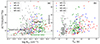 |
Fig. 12. (a) Relation between X(13CO)/X(C18O) and N(13CO). The red, blue, green, and gray dots correspond to pixels in the W5-E1, W5-M, W5-W1 and W5-W2 regions, respectively. The gray dashed rectangles delineate the principal distribution areas within the Planck cold clumps (Wu et al. 2012), and the Orion molecular clouds (Shimajiri et al. 2014), corresponding to type I and typeII molecular clouds (Wang et al. 2019), respectively. The green line indicates the terrestrial ratio X(13CO)/X(C18O) = 5.5 (Wilson & Matteucci 1992). (b) Relation between X(13CO)/X(C18O) and Tex. Note that only those pixels with both detectable (larger than 3σ) 13CO and C18O emissions are plotted. |
5.1.2. Stacked average spectra under different feedback conditions
Polycyclic aromatic hydrocarbons (PAHs) typically trace the boundary between the ionized and neutral gas in molecular clouds (Rathborne et al. 2002), known as photodissociation or PDRs. The PAHs absorb FUV radiation from hot stars and re–emit fluorescently in several broad bands at near and mid-infrared (IR) wavelengths (Allamandola et al. 1989; Tielens 2008). The most luminous of these are within the 6–13 μm range (e.g. Fazio et al. 2004), so we use the 8.28 μm line from the MSX to distinguish regions that are affected by feedback due to the star’s FUV radiation. The green portion of the RGB plot in Fig. 1 represents the distribution of the feedback region described by the 8 μm radiation. In this section, we investigate the effect of feedback on the line profiles of the W5 molecular cloud complex, especially whether the shape of the line profiles in the regions where we expect feedback to be present is significantly different from those where we see little evidence for feedback.
Different 8 μm intensities represent different levels of feedback, and we give different threshold values to distinguish different feedback effects. We defined the region with an 8 μm flux above the threshold of 1.1 × 10⁻⁶ W/(m−2⋅ sr) as the “feedback region,” and divided the values between the threshold and the maximum 8 μm flux into nine parts for each of the four regions (W5-E1, W5-M, W5-W1, and W5-W2) to analyze the effects of different feedback levels. The threshold value for each region is presented in the upper-left corner of the respective region’s subplot in Fig. 13. Regions (pixels) with 8 μm flux densities higher than a specific threshold were labeled as “inside feedback regions” and those below the threshold were labeled “outside feedback regions.” Before obtaining the stacked average spectral lines, we first smoothed the 8 μm radiation from MSX to the same resolution (51″) and pixel size (30″) as the 13CO emission. Given an 8 μm threshold, and that all 13CO molecular lines used must be above the 3σ level, the average of all 13CO lines at all locations (pixels) greater than the threshold represents the feedback region, and the average spectral line at all other locations arises from the non-feedback region.
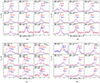 |
Fig. 13. Stacked spectra of 13CO (J = 1–0) emission corresponding to the “inside” (red) and “outside feedback” zones (blue) for different choices of MSX at 8.28 μm flux density (designated as “thre” in units of W/(m−2⋅ sr) in the top–left of each subplot) in the four regions: W5-E1, W5-M, W5-W1, and W5-W2, as described in Fig. 8. The red solid and blue dotted lines in all the subplots correspond to the position of peak emission of the average stacked spectra inside and outside the feedback zone with MSX 8.28 μm flux densities above and below the variation threshold. The velocity interval between the two peak lines is expressed in “ dv” ( km s−1) on the top–left of each subplot. (a) W5-E1, (b) W5-M, (c) W5-W1, (d) W5-W2. |
Figure 13 shows the averaged stacked 13CO spectra corresponding to the “inside-” and “outside feedback zones” for the W5 molecular cloud complex in four different sub-regions (W5-E1, W5-M, W5-W1, W5-W2). The average spectrum in red corresponds to the “feedback region,” which includes the average spectrum of all 13CO lines for pixel points within the entire interval where the 8 μm flux exceeds a specified threshold. The average spectrum for all other points, represented in blue, corresponds to the “non-feedback region.” The red dashed and the blue dashed lines, respectively, indicate the peak positions of the two average spectra, with their corresponding velocity values marked. The term “dv” represents the difference between the velocity of the peak in the feedback region spectrum and the velocity of the peak in the non-feedback region spectrum.
There are several distinct features in Fig. 13. The spectra from the “inside feedback zones” are brighter than the “outside feedback zones” for all four regions. With increasing feedback strength the peaks of the former also get brighter indicating that feedback primarily occurs in denser regions, where star formation is more active. This may be due to dense gas attenuating the radiation from central OB stars, causing the radiation to excite these dense areas. The average spectrum profiles for the “inside feedback zones” and the “outside feedback zones” in the four regions appear very different from each other, as they are indeed representative of the actual differences between the two regions.
In the W5-E1 and W5-W2 regions, with increasing 8 μm threshold, the peak of the average 13CO spectrum in the “inside feedback” region exhibits a noticeable redshift relative to the peak in the “outside feedback” region spectrum. This shift is also clearly evident in the changing values of “dv”. On the contrary, W5-M exhibits a completely opposite trend, wherein the spectrum from the “inside feedback” region shows a distinct blueshift relative to the spectrum from the “outside feedback” region as the threshold increases. W5-W1 exhibits entirely different characteristics compared to the three aforementioned regions. It inherently possesses two distinct velocity components separated by approximately 3 km s−1, denoted as v1 (about –40 km s−1) and v2 (about –37 km s−1). With the increase in threshold, v1 shows a slight redshift, while v2 undergoes minimal change. Furthermore, the analysis of the result of NH3 in Sect. 3.2 indicates that W5-W1 comprises three distinct velocity components, with v1 situated on the side closer to the center of W5, and v2 located on the side farther from the center. These results indicate that molecular gas on the side closer to the center of the two HII regions exhibits stronger 8 μm radiation and is notably influenced by this radiation. These findings seemingly provide ample evidence for the influence of supersonic expansion from the central HII region in the W5 complex on W5-E1, W5-M, and W5-W1. In contrast, W5-W2 may be influenced by radiation from IC 1805 (in W4) (Moffat 1972).
5.2. Effects of feedback on clumps
The feedback effect from newly formed stars has been verified by changes in the excitation temperature, column density, and distribution of spectral lines of the molecular clouds. Therefore the question arises whether this effect has consequences for the star-forming activity in denser regions. This requires an analysis of the physical parameters of the clump structure.
5.2.1. Mass-radius and virial mass versus LTE mass relation
To examine how many clumps have the potential to form high-mass stars, we present the mass–size relation of the 13CO clumps in the left panel of Fig. 14. The red and green dots in Fig. 11 represent the class I and class II YSOs established by Koenig et al. (2008). It is evident from their distribution that class I YSOs are spatially connected with molecular clumps, while class II YSOs tend to be located farther away and are mostly concentrated near the centers of the two HII regions. This may be due to the fact that the HII regions initially trigger star formation at their centers, resulting in younger YSOs at the radii presently occupied by molecular gas.
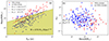 |
Fig. 14. (a) Mass and radius relationships for all identified 13CO clumps. The red and blue dots correspond to clumps that respectively contain and do not contain class I YSOs. The distribution of YSOs is illustrated in Fig. 11. The black, red, and blue dashed lines represent the best power-law fits for the mass-radius relationship for all clumps, YSOs clumps, and no YSOs clumps, respectively. The yellow area denotes the empirically derived parameter set m(r) < 870 M⊙(r/pc)1.33, where massive star formation should not occur (Kauffmann & Pillai 2010). (b) Virial mass relationships for all 13CO clumps, The black dashed lines correspond to positions with virial values of 1 and 2. Values below unity represent the gravitationally bound state and values above two indicate a gravitationally unbound state, respectively (see also Eq. (17)). |
Based on the distribution of class I YSOs, we categorized the identified clumps into “YSO clumps” and “non YSO clumps,” differentiated by the red and blue colors in Fig. 14. The dashed black line denotes the empirically derived threshold m(r) = 870 M⊙(r/pc)1.33 above which massive star formation can be expected (Kauffmann & Pillai 2010). About 26.4% (56 of 212) of the clumps tend to be above this threshold, indicating that they will likely form high-mass stars, reflecting the strong star-formation activity in this region. 25.5% (54 of 212) clumps belong to the “YSO clumps,” and they are predominantly distributed above the threshold for high-mass star formation. Combining this distribution with the spatial arrangement of YSOs suggests that high-mass stars primarily form on the dense layers at the boundaries of HII regions, consistent with the findings of Keown et al. (2019).
The right panel of Fig. 14 shows observed αvir and MLTE for all clumps in our final catalog. Of the 212 clumps, 53 (25%) fall below the αvir = 1 threshold to be considered to be gravitationally bound, and 38 (17.9%) in the range 1 < αvir < 2. It is evident that “YSO clumps” are generally distributed in the lower-right quadrant (56% (31/54) of the “YSO clumps” and 37% (60/158) of the “non-YSO clumps” are characterized by virial parameters below two). Their lower virial value indicates that gravity effects are stronger so that it is more likely that the clump will collapse to form a core, while many authors specifically study this process in detail using ALMA (e.g. Tan et al. 2013; Indebetouw et al. 2013; Rathborne et al. 2015; Tang et al. 2019, 2021; Li et al. 2020b; Henkel et al. 2022). We find that the virial parameters of the 13CO clumps tend to decrease with increasing LTE masses. This indicates that 13CO clumps with larger LTE masses are more likely to be gravitationally bound. At the same time, there exists a power-law relationship between mass and radius in Fig. 14(a), wherein larger clumps generally exhibit lower virial values in Fig. 14(b). This aligns with the views presented in Goodman et al. (2009a), suggesting that self-gravitating structures appear to be more widespread on larger scales than on smaller ones when considering the material traced by 13CO observations. At densities surpassing 5 × 103 cm−3, 13CO becomes an increasingly poor tracer of mass (Goodman et al. 2009b), so it can only provide upper limits for the “true” virial parameters of the densest, most compact, structures seen in the dendrogram (Goodman et al. 2009a). The clumps with low virial values are basically located in the densest part, indicating that the star formation activity at these positions is the most intense. These clumps will preferentially form stars under the action of gravity. They are more likely to accrete more material to sustain their growth than clumps exposed to weaker gravitational forces. So they are more likely forming massive stars.
5.2.2. Feedback from two large H II regions
To analyze the effect of radiation from the central massive stars on the evolutionary state of the molecular clouds, we used the method in Sect. 5.1.2, where all clumps that have pixels with 8 μm flux larger than a given threshold (1.1 × 10⁻⁶ W/(m−2⋅ sr) in 8 μm flux) are defined as “feedback clumps,” while the other clumps below this threshold are defined as “non-feedback clumps.” Fig. 15 shows the spatial distribution of these clumps after classification. It is obvious that feedback clumps are almost all distributed on the side close to the central stellar clusters in W5. Additionally, feedback clumps are also distributed along the western edge of W5-W2. According to Karr & Martin (2003), W5-W2 is believed to be influenced by the expansion and radiation from the super-large HII region W4 (its center position is longitude = 134.83°, latitude = 0.95°, and has the configuration of a large shell, roughly 1° × 1.5° in angular size Megeath et al. 2008). In W5, the percentage of the feedback-clumps is 50.9% (108 feedback clumps among a total of 212 clumps).
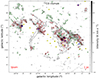 |
Fig. 15. Distribution of “feedback clumps” and “non-feedback clumps” classified under the 8 μm threshold 1.1 × 10⁻⁶ W/(m−2⋅ sr). The gray background image represents the integrated intensity map of 13CO, while the black contour lines depict the above mentioned 8 μm flux intensity. Red contours denote 13CO-identified clumps that are classified as “feedback clumps”, while Green contours show all other 13CO-identified clumps, the so-called “non-feedback clumps.” The yellow stars and blue crosses correspond to OB stars (Roman-Lopes et al. 2019) and HMYSOs (Lumsden et al. 2013), respectively. |
Fig. 16 shows the distribution of the “feedback clump” parameters in relation to the 8 μm flux in the W5 complex. Mazumdar et al. (2021a) found that the surface mass density of the leaves and branches increases with increasing 8 μm flux in the G305 molecular complex, indicating that in regions of stronger feedback, the clumps are more massive. Our results also show this trend but are deduced making use of more clump parameters. Results reveal that parameters such as mass, density, excitation temperature, luminosity, velocity dispersion, as well as the thermal, and non-thermal velocity dispersion, increase with stronger 8 μm flux. However, the virial parameter exhibits a slightly decreasing trend, while the luminosity-to-mass ratio remains relatively constant. These phenomena are sufficient to indicate that the feedback effect from OB stars favors larger clumps of higher density. Excitation temperature and velocity dispersion are also enhanced, and the clumps tend to become gravitationally unstable.
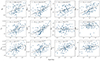 |
Fig. 16. Parameters of the “feedback clumps” in relation to the intensity of the 8 μm flux. Grey lines show the results of a power law fit to these quantities for clumps. |
We assume that clumps in the non-feedback region represent an earlier state of the molecular clouds. To estimate the effect of feedback from the W5 central OB star on the evolution of the clumps, we compare the difference between the “feedback clump” and “non-feedback clump” parameters. The αvir-mass relation of Fig. 17(a) clearly distinguishes “feedback clumps” from “non-feedback clumps.” In particular, the clumps in the feedback region are mostly distributed in regions with higher mass, specifically in proximity to the boundaries of the W5 HII regions. Fig. 17(b) gives the Cumulative Distribution Function (CDF) of the two types of clumps. The results clearly distinguish between these; namely, the “feedback clumps” show a much flatter CDF than the “non-feedback clump.” Figure 18 shows the difference between all parameters of the two types of clumps, almost all of which have a clear separation. Feedback clumps exhibit significantly higher densities, higher temperatures, higher thermal and non-thermal velocity dispersions, and slightly lower virial values compared to “non-feedback clumps.” These results suggest that the triggering mechanism plays a decisive role in the star-forming activity of the W5 molecular cloud.
 |
Fig. 17. (a) Virial parameter (α) vs. mass for the clumps in the feedback (red dots) and non-feedback (blue dots) regions. The black dashed lines are the same as in Fig. 14. (b) Cumulative distribution function (CDF) of mass between feedback (red line) and non-feedback region (blue line). |
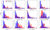 |
Fig. 18. Comparison of clump parameters of “feedback” and “non-feedback clumps” in the W5 complex. |
5.2.3. Feedback from outflows inside the molecular gas
In the simulations, outflow effects are capable of maintaining the turbulence within parsec-scale clumps that are already forming stars. These clumps break down into even denser “cores” that are believed to be the immediate precursors of single or gravitationally bound multiple massive protostars. The high-velocity dispersions of these clumps are generally interpreted as strong turbulence that supports the clumps against gravity (Lizano & Osorio 1999; McKee & Tan 2003). Maud et al. (2015) and Yang et al. (2018) suggested that these outflows have enough power to drive turbulence in the local environment, but do not contribute significantly to the overall turbulence of the clouds.
In order to verify the effect of turbulence generated by outflows on the clump’s evolution, we matched the outflow candidates identified by Li et al. (2019) with the clumps we identified, and classified the clumps as “outflow” or as “non-outflow” clumps, depending on their location. According to the above method, 81 (38.2%) clumps are defined as “outflow clumps” and the other 131 (61.8%) clumps are “non-outflow clumps.” The distribution of the clumps is given in Fig. 19.
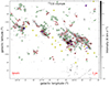 |
Fig. 19. Distribution of “outflow clumps” and “non-outflow clumps” classified according to whether there is an outflow (Li et al. 2019) inside a given clump. Red contours denote 13CO-identified clumps that are classified as “outflow clumps,” while green contours show all other 13CO-identified clumps as “non-outflow clumps.” The gray background image, yellow stars and blue crosses are the same as in Fig. 15. The small black dots correspond to CO outflows identified by Li et al. (2019). |
In order to study the effect of different outflow energies on the evolution of clumps, we show the relationship between clump parameters and outflow energy in each clump (Li et al. 2019) in Fig. 20.
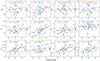 |
Fig. 20. Parameters of the “outflow clumps” in relation to the energy of the outflow inside the clump. Grey lines show the results of a power law fit to these quantities for clumps. |
The results indicate that nearly all parameter relationships exhibit a similar trend as the “feedback clumps.” However, parameters such as mass density, virial parameter, and luminosity-mass ratio display a notably weaker correlation. This could be attributed to the fact that outflows are not exclusively distributed within dense active massive star-forming zones; they are also present in more quiescent, namely, areas of low mass star formation, leading to a more complex distribution. Furthermore, the non-thermal velocity dispersion demonstrates a steeper trend compared to the thermal velocity dispersion. This suggests that the turbulence within the clumps is primarily sustained by outflows, rather than being significantly influenced by the thermal velocity component.
In addition, we give the parameter distinction between “outflow clumps” and “non-outflow clumps” in Figs. 21 and 22. Similarly to the case with feedback, the αvir-mass relation and the cumulative distribution function (CDF) show a significantly different distribution in the two types of clumps. The parameter distribution of Fig. 22 also shows a distinctly different distribution. The “Outflow clumps” usually have higher density, mass, temperature, higher thermal velocity dispersion, and lower virial value. Unlike our findings for the feedback and non-feedback regions, the outflow clumps tend to have a higher L/M value, which means that these clumps are later in evolution (Molinari et al. 2008; Urquhart et al. 2018), while the clumps in the feedback region seem to continue the global accretion of matter under the action of feedback.
6. Summary
Using CO data from the survey MWISP project, we studied the gas structure distribution of the W5 molecular clouds complex and the feedback effect of OB stars at the center of the two bubbles on molecular cloud gas. To analyze the effects of feedback and outflow on star formation in molecular clouds, we identified clumps on 13CO cube data and performed a detailed analysis of these clump parameters. As a complement, we performed NH3(1,1) and NH3(2,2) line observations for the four densest zones on the boundary of the HII region in W5 to analyze additional physical parameters. Our main results and conclusions are summarized below.
1. From the morphology of CO, we can see that the gas is mainly distributed near the boundary of the two main ionized bubbles. However, in W5-M, we find that C18O shows almost no signal. With respect to CO, we find a higher Tex compared with other regions. From the column density and the distribution of Tex, it is further confirmed that the CO molecular gas in W5 is significantly affected by the presence of the two ionized bubbles.
2. Comparing the values of Tkin from ammonia and Tex from carbon monoxide, it is observed that AFGL 4029 exhibits higher Tex and lower Tkin values, whereas W5-W1 displays the opposite trend. This indicates that optically thick CO alone might not be sufficient for accurately calculating parameters in the dense regions.
3. Following the intensity relationship between NH3(1,1) and C18O, we find that AFGL 4029 is characterized by a lower Tkin and higher column density, while the W5-W1 area shows the opposite behavior. In W5-W1, C18O has a higher intensity relative to ammonia, indicating that in this environment, CO no longer freezes on the surface of the dust particles but evaporates.
4. Based on the calculated CO column density distribution, four denser regions were identified, namely W5-E1, W5-M, W5-W1, and W5-W2. Following the 13CO/C18O abundance ratio relationship with N13 and Tex as presented in Wang et al. (2019), it is evident that W5-E1, W5-M, and W5-W1 belong to type I clouds, while W5-W2 belong to type II.
5. The region showing 8 μm PAH emission is identified as the feedback region. Given different flux thresholds, it is found that the peak of the stacked average spectral line of CO has an obvious redshift or blue shift compared with the average spectral line of the non-feedback region, suggesting that the feedback from the OB stars near the center of the bubbles affects the motion of the gas, thereby promoting the evolution of the molecular cloud.
6. Searching for 13CO clumps in the W5 region, a total of 212 clumps have been found. Based on the mass-radius relationship and the virial-mass relationship, about 26.4% (56) of the clumps were found to have the ability to form massive stars and 42.9% (91) of the clumps appear to be gravitationally bound. Within these clumps capable of forming high-mass stars, there is a distribution of class I YSOs, all located in dense regions near the boundary of the HII region.
7. Using 8 μm radiation to quantify a specific threshold 1.1 × 10⁻⁶ W/(m−2⋅ sr), clumps with an internal 8 μm flux greater than the threshold are classified as “Feedback clumps,” and other sources are “non-feedback clumps.” The stronger the 8 μm flux density, the greater the mass of the clump. Tex, luminosity, thermal velocity dispersion, non-thermal velocity dispersion, and other parameters show a clearly increasing trend, while the virial parameter shows a clear downward trend, which suggests that accretion activity may be stronger in such cases.
8. According to whether there are molecular outflows related to a specific clump, clumps are classified as “outflow clumps” or “non-outflow clumps.” Similarly to the “feedback clump” case, the parameters of “outflow clumps” indicate a strong correlation with the clump’s outflow energy and are significantly different from “non-outflow clumps.” The only difference is that the L/M of the “feedback clumps” has no significant correlation with the 8 μm flux, while the L/M of the “outflow clumps” has a slightly positive relationship with the outflow energy inside the clumps.
In summary, CO and NH3 provide ample evidence that the molecular complex in the W5 region is strongly affected by the OB stars at the centers of the bubbles.
Data availability
Full Table 1 is available at the CDS via anonymous ftp to cdsarc.cds.unistra.fr (130.79.128.5) or via https://cdsarc.cds.unistra.fr/viz-bin/cat/J/A+A/689/A140
A community-developed core Python package and an ecosystem of tools and resources for astronomy http://www.astropy.org
GILDAS is a collection of state-of-the-art software oriented toward (sub-)millimeter radioastronomical applications (for both single-dish and interferometric data) https://iram.fr/IRAMFR/GILDAS/.
Non-LTE molecular radiative transfer in an isothermal homogeneous medium https://var.sron.nl/radex/radex.php
Astrodendro is a Python package for computing dendrograms of astronomical data http://www.dendrograms.org/
Acknowledgments
We like to thank the anonymous referee for the useful suggestions that improved this study. This work was mainly funded by the National Key R&D Program of China under grant No. 2022YFA1603103. It was also partially funded by the Regional Collaborative Innovation Project of Xinjiang Uyghur Autonomous Region under grant No. 2022E01050, the National Natural Science Foundation of China (NSFC) under grants Nos. 12173075, 12373029, and 12103082, the Tianshan Talent Program of Xinjiang Uygur Autonomous Region under grant No. 2022TSYCLJ0005, Tianchi Talents Program of Xinjiang Uygur Autonomous Region, the Natural Science Foundation of Xinjiang Uygur Autonomous Region under grant No. 2022D01E06, the Chinese Academy of Sciences (CAS) “Light of West China” Program under grants Nos. xbzg-zdsys-202212, 2020-XBQNXZ-017, and 2021-XBQNXZ-028, the National Key R&D Program of China with grant 2023YFA1608002, and the Xinjiang Key Laboratory of Radio Astrophysics under grant No. 2022D04033. D.L. acknowledges support from Youth Innovation Promotion Association CAS. C.H. has been funded by the Chinese Academy of Sciences President’s International Fellowship Initiative by grant No. 2023VMA0031. Moreover, this work is partially funded by the Science Committee of the Ministry of Science and Higher Education of the Republic of Kazakhstan grant No. AP13067768. This study uses the data from the Galaxy Picture Survey Project. MWISP is sponsored by the National Key R&D Program of China with grant 2023YFA1608000 and the CAS Key Research Program of Frontier Sciences with grant QYZDJ-SSW-SLH047. The Purple Mountain Observatory 13.7 telescope is used to carry out the north Galactic plane 12CO/13CO/C18O multispectral line survey. Thanks to the long-term work of the working group, especially the staff of the Qinghai Observation Station. The NanShan 26-m Radio Telescope is partly supported by the Operation, Maintenance, and Upgrading Fund for Astronomical Telescopes and Facility Instruments, budgeted by the Ministry of Finance of China (MOF) and administrated by the Chinese Academy of Sciences (CAS), and the Urumqi NanShan Astronomy and Deep Space Exploration Observation and Research Station of Xinjiang.
References
- Allamandola, L. J., Tielens, A. G. G. M., & Barker, J. R. 1989, ApJS, 71, 733 [Google Scholar]
- Anderson, L. D., Bania, T. M., Balser, D. S., et al. 2014, ApJS, 212, 1 [Google Scholar]
- Areal, M. B., Paron, S., Ortega, M. E., & Duvidovich, L. 2019, PASA, 36, e049 [NASA ADS] [CrossRef] [Google Scholar]
- Bertoldi, F. 1989, ApJ, 346, 735 [Google Scholar]
- Bertoldi, F., & McKee, C. F. 1990, ApJ, 354, 529 [NASA ADS] [CrossRef] [Google Scholar]
- Brunt, C. M. 2010, A&A, 513, A67 [NASA ADS] [CrossRef] [EDP Sciences] [Google Scholar]
- Camacho, M., Edwards, B., & Engheta, N. 2020, Nat. Commun., 11, 3733 [NASA ADS] [CrossRef] [Google Scholar]
- Dame, T. M., Hartmann, D., & Thaddeus, P. 2001, ApJ, 547, 792 [Google Scholar]
- Danby, G., Flower, D. R., Valiron, P., Schilke, P., & Walmsley, C. M. 1988, MNRAS, 235, 229 [NASA ADS] [CrossRef] [Google Scholar]
- Deharveng, L., Zavagno, A., Anderson, L. D., et al. 2012, A&A, 546, A74 [NASA ADS] [CrossRef] [EDP Sciences] [Google Scholar]
- Elmegreen, B. G., & Lada, C. J. 1977, ApJ, 214, 725 [Google Scholar]
- Fazio, G. G., Hora, J. L., Allen, L. E., et al. 2004, ApJS, 154, 10 [Google Scholar]
- Frerking, M. A., Langer, W. D., & Wilson, R. W. 1982, ApJ, 262, 590 [Google Scholar]
- Garden, R. P., Hayashi, M., Gatley, I., Hasegawa, T., & Kaifu, N. 1991, ApJ, 374, 540 [NASA ADS] [CrossRef] [Google Scholar]
- Glassgold, A. E., Huggins, P. J., & Langer, W. D. 1985, ApJ, 290, 615 [NASA ADS] [CrossRef] [Google Scholar]
- Goldsmith, P. F., & Langer, W. D. 1999, ApJ, 517, 209 [Google Scholar]
- Goldsmith, P. F., Heyer, M., Narayanan, G., et al. 2008, ApJ, 680, 428 [Google Scholar]
- González-Samaniego, A., & Vazquez-Semadeni, E. 2020, MNRAS, 499, 668 [CrossRef] [Google Scholar]
- Goodman, A. A., Rosolowsky, E. W., Borkin, M. A., et al. 2009a, Nature, 457, 63 [NASA ADS] [CrossRef] [Google Scholar]
- Goodman, A. A., Pineda, J. E., & Schnee, S. L. 2009b, ApJ, 692, 91 [Google Scholar]
- Hacar, A., Alves, J., Burkert, A., & Goldsmith, P. 2016, A&A, 591, A104 [NASA ADS] [CrossRef] [EDP Sciences] [Google Scholar]
- Henkel, C., Walmsley, C. M., & Wilson, T. L. 1980, A&A, 82, 41 [NASA ADS] [Google Scholar]
- Henkel, C., Wilson, T. L., & Bieging, J. 1982, A&A, 109, 344 [NASA ADS] [Google Scholar]
- Henkel, C., Wilson, T. L., Walmsley, C. M., & Pauls, T. 1983, A&A, 127, 388 [NASA ADS] [Google Scholar]
- Henkel, C., Guesten, R., & Gardner, F. F. 1985, A&A, 143, 148 [Google Scholar]
- Henkel, C., Wilson, T. L., Langer, N., Chin, Y. N., & Mauersberger, R. 1994, Lect. Notes Phys., 439, 72 [NASA ADS] [CrossRef] [Google Scholar]
- Henkel, C., Menten, K. M., Murphy, M. T., et al. 2012, in Twelfth Marcel Grossmann Meeting on General Relativity, ed. A. H. Chamseddine (World Scientific Publishing Co. Pte. Ltd.), 1500 [CrossRef] [Google Scholar]
- Henkel, C., Hunt, L. K., & Izotov, Y. I. 2022, Galaxies, 10, 11 [NASA ADS] [CrossRef] [Google Scholar]
- Ho, P. T. P., & Townes, C. H. 1983, ARA&A, 21, 239 [NASA ADS] [CrossRef] [Google Scholar]
- Hollenbach, D. J., & Tielens, A. G. G. M. 1997, ARA&A, 35, 179 [NASA ADS] [CrossRef] [Google Scholar]
- Hollenbach, D. J., Takahashi, T., & Tielens, A. G. G. M. 1991, ApJ, 377, 192 [NASA ADS] [CrossRef] [Google Scholar]
- Indebetouw, R., Brogan, C., Chen, C. H. R., et al. 2013, ApJ, 774, 73 [NASA ADS] [CrossRef] [Google Scholar]
- Karr, J. L., & Martin, P. G. 2003, ApJ, 595, 900 [NASA ADS] [CrossRef] [Google Scholar]
- Kauffmann, J., & Pillai, T. 2010, ApJ, 723, L7 [Google Scholar]
- Kawamura, J. H., & Masson, C. R. 1998, ApJ, 509, 270 [NASA ADS] [CrossRef] [Google Scholar]
- Keown, J., Di Francesco, J., Rosolowsky, E., et al. 2019, ApJ, 884, 4 [Google Scholar]
- Koenig, X. P., Allen, L. E., Gutermuth, R. A., et al. 2008, ApJ, 688, 1142 [NASA ADS] [CrossRef] [Google Scholar]
- Kong, S., Lada, C. J., Lada, E. A., et al. 2015, ApJ, 805, 58 [NASA ADS] [CrossRef] [Google Scholar]
- Langer, W. D., Graedel, T. E., Frerking, M. A., & Armentrout, P. B. 1984, ApJ, 277, 581 [Google Scholar]
- Li, Y., Xu, Y., Yang, J., et al. 2015, AJ, 150, 60 [NASA ADS] [CrossRef] [Google Scholar]
- Li, Y., Xu, Y., Sun, Y., et al. 2019, ApJS, 242, 19 [NASA ADS] [CrossRef] [Google Scholar]
- Li, Y., Xu, Y., Sun, Y., & Yang, J. 2020a, ApJS, 251, 26 [NASA ADS] [CrossRef] [Google Scholar]
- Li, D., Tang, X., Henkel, C., et al. 2020b, ApJ, 901, 62 [NASA ADS] [CrossRef] [Google Scholar]
- Lin, Z., Sun, Y., Xu, Y., Yang, J., & Li, Y. 2021, ApJS, 252, 20 [NASA ADS] [CrossRef] [Google Scholar]
- Liszt, H. S. 2007, A&A, 476, 291 [NASA ADS] [CrossRef] [EDP Sciences] [Google Scholar]
- Liu, T., Wu, Y., Zhang, H., & Qin, S.-L. 2012, ApJ, 751, 68 [NASA ADS] [CrossRef] [Google Scholar]
- Lizano, S., & Osorio, M. 1999, in Wolf-Rayet Phenomena in Massive Stars and Starburst Galaxies, eds. K. A. van der Hucht, G. Koenigsberger, & P. R. J. Eenens (San Francisco, California: Astronomical Society of the Pacific), 193, 559 [NASA ADS] [Google Scholar]
- Lumsden, S. L., Hoare, M. G., Urquhart, J. S., et al. 2013, ApJS, 208, 11 [Google Scholar]
- MacLaren, I., Richardson, K. M., & Wolfendale, A. W. 1988, ApJ, 333, 821 [NASA ADS] [CrossRef] [Google Scholar]
- Mao, R. Q., Henkel, C., Schulz, A., et al. 2000, A&A, 358, 433 [NASA ADS] [Google Scholar]
- Maud, L. T., Moore, T. J. T., Lumsden, S. L., et al. 2015, MNRAS, 453, 645 [Google Scholar]
- Mauersberger, R., Henkel, C., Wilson, T. L., & Walmsley, C. M. 1986, A&A, 162, 199 [Google Scholar]
- Mazumdar, P., Wyrowski, F., Urquhart, J. S., et al. 2021a, A&A, 656, A101 [NASA ADS] [CrossRef] [EDP Sciences] [Google Scholar]
- Mazumdar, P., Wyrowski, F., Colombo, D., et al. 2021b, A&A, 650, A164 [NASA ADS] [CrossRef] [EDP Sciences] [Google Scholar]
- McKee, C. F., & Tan, J. C. 2003, ApJ, 585, 850 [Google Scholar]
- Megeath, S. T., Townsley, L. K., Oey, M. S., & Tieftrunk, A. R. 2008, Handbook of Star Forming Regions, Volume I (The Northern Sky ASP Monograph Publications), 4, 264 [NASA ADS] [Google Scholar]
- Minchin, N. R., White, G. J., & Ward-Thompson, D. 1995, A&A, 301, 894 [NASA ADS] [Google Scholar]
- Moffat, A. F. J. 1972, A&AS, 7, 355 [NASA ADS] [Google Scholar]
- Molinari, S., Pezzuto, S., Cesaroni, R., et al. 2008, A&A, 481, 345 [NASA ADS] [CrossRef] [EDP Sciences] [Google Scholar]
- Mühle, S., Seaquist, E. R., & Henkel, C. 2007, ApJ, 671, 1579 [NASA ADS] [CrossRef] [Google Scholar]
- Myers, P. C. 1983, ApJ, 270, 105 [Google Scholar]
- Niwa, T., Tachihara, K., Itoh, Y., et al. 2009, A&A, 500, 1119 [NASA ADS] [CrossRef] [EDP Sciences] [Google Scholar]
- Ott, J., Henkel, C., Staveley-Smith, L., & Weiß, A. 2010, ApJ, 710, 105 [NASA ADS] [CrossRef] [Google Scholar]
- Pineda, J. E., Caselli, P., & Goodman, A. A. 2008, ApJ, 679, 481 [Google Scholar]
- Pineda, J. L., Goldsmith, P. F., Chapman, N., et al. 2010, ApJ, 721, 686 [NASA ADS] [CrossRef] [Google Scholar]
- Rathborne, J. M., Burton, M. G., Brooks, K. J., et al. 2002, MNRAS, 331, 85 [NASA ADS] [CrossRef] [Google Scholar]
- Rathborne, J. M., Longmore, S. N., Jackson, J. M., et al. 2015, ApJ, 802, 125 [Google Scholar]
- Röllig, M., & Ossenkopf, V. 2013, A&A, 550, A56 [NASA ADS] [CrossRef] [EDP Sciences] [Google Scholar]
- Roman-Lopes, A., Román-Zúñiga, C. G., Tapia, M., et al. 2019, ApJ, 873, 66 [NASA ADS] [CrossRef] [Google Scholar]
- Rosolowsky, E., & Leroy, A. 2006, PASP, 118, 590 [NASA ADS] [CrossRef] [Google Scholar]
- Shan, W., Yang, J., Shi, S., et al. 2012, IEEE Trans. Terahertz Sci. Technol., 2, 593 [Google Scholar]
- Shimajiri, Y., Kitamura, Y., Saito, M., et al. 2014, A&A, 564, A68 [NASA ADS] [CrossRef] [EDP Sciences] [Google Scholar]
- Shirley, Y. L. 2015, PASP, 127, 299 [Google Scholar]
- Shu, F. H., Adams, F. C., & Lizano, S. 1987, ARA&A, 25, 23 [Google Scholar]
- Su, Y., Yang, J., Zhang, S., et al. 2019, ApJS, 240, 9 [Google Scholar]
- Sun, Y., Yang, J., Xu, Y., et al. 2020, ApJS, 246, 7 [NASA ADS] [CrossRef] [Google Scholar]
- Suri, S., Sánchez-Monge, Á., Schilke, P., et al. 2019, A&A, 623, A142 [NASA ADS] [CrossRef] [EDP Sciences] [Google Scholar]
- Tafalla, M., Myers, P. C., Caselli, P., Walmsley, C. M., & Comito, C. 2002, ApJ, 569, 815 [Google Scholar]
- Tafalla, M., Myers, P. C., Caselli, P., & Walmsley, C. M. 2004, A&A, 416, 191 [NASA ADS] [CrossRef] [EDP Sciences] [Google Scholar]
- Takekoshi, T., Fujita, S., Nishimura, A., et al. 2019, ApJ, 883, 156 [NASA ADS] [CrossRef] [Google Scholar]
- Tan, J. C., Kong, S., Butler, M. J., Caselli, P., & Fontani, F. 2013, ApJ, 779, 96 [Google Scholar]
- Tang, X. D., Henkel, C., Menten, K. M., et al. 2019, A&A, 629, A6 [NASA ADS] [CrossRef] [EDP Sciences] [Google Scholar]
- Tang, X. D., Henkel, C., Menten, K. M., et al. 2021, A&A, 655, A12 [NASA ADS] [CrossRef] [EDP Sciences] [Google Scholar]
- Tielens, A. G. G. M. 2008, ARA&A, 46, 289 [NASA ADS] [CrossRef] [Google Scholar]
- Tielens, A. G. G. M., & Hollenbach, D. 1985, ApJ, 291, 722 [Google Scholar]
- Townes, C. H., Genzel, R., Watson, D. M., & Storey, J. W. V. 1983, ApJ, 269, L11 [CrossRef] [Google Scholar]
- Tursun, K., Esimbek, J., Henkel, C., et al. 2020, A&A, 643, A178 [NASA ADS] [CrossRef] [EDP Sciences] [Google Scholar]
- Urquhart, J. S., König, C., Giannetti, A., et al. 2018, MNRAS, 473, 1059 [Google Scholar]
- van der Tak, F. F. S., Black, J. H., Schöier, F. L., Jansen, D. J., & van Dishoeck, E. F. 2007, A&A, 468, 627 [NASA ADS] [CrossRef] [EDP Sciences] [Google Scholar]
- van Dishoeck, E. F., & Black, J. H. 1988, ApJ, 334, 771 [Google Scholar]
- Vázquez-Semadeni, E., González-Samaniego, A., & Colín, P. 2017, MNRAS, 467, 1313 [NASA ADS] [Google Scholar]
- Vázquez-Semadeni, E., Palau, A., Ballesteros-Paredes, J., Gómez, G. C., & Zamora-Avilés, M. 2019, MNRAS, 490, 3061 [Google Scholar]
- Walmsley, C. M., & Ungerechts, H. 1983, A&A, 122, 164 [Google Scholar]
- Wang, C., Yang, J., Su, Y., et al. 2019, ApJS, 243, 25 [NASA ADS] [CrossRef] [Google Scholar]
- Whitworth, A. P., Bhattal, A. S., Chapman, S. J., Disney, M. J., & Turner, J. A. 1994, MNRAS, 268, 291 [Google Scholar]
- Wienen, M., Wyrowski, F., Schuller, F., et al. 2012, A&A, 544, A146 [NASA ADS] [CrossRef] [EDP Sciences] [Google Scholar]
- Wilson, T. L., & Matteucci, F. 1992, A&ARv, 4, 1 [Google Scholar]
- Wilson, T. L., & Rood, R. 1994, ARA&A, 32, 191 [Google Scholar]
- Wilson, T. L., Rohlfs, K., & Hüttemeister, S. 2009, Tools of Radio Astronomy (Germany: Springer-Verlag, Berlin) [Google Scholar]
- Wu, Y., Liu, T., Meng, F., et al. 2012, ApJ, 756, 76 [CrossRef] [Google Scholar]
- Wu, G., Qiu, K., Esimbek, J., et al. 2018, A&A, 616, A111 [NASA ADS] [CrossRef] [EDP Sciences] [Google Scholar]
- Xu, Y., Reid, M. J., Zheng, X. W., & Menten, K. M. 2006, Science, 311, 54 [NASA ADS] [CrossRef] [Google Scholar]
- Yamagishi, M., Hara, C., Kawabe, R., et al. 2019, ApJ, 875, 62 [NASA ADS] [CrossRef] [Google Scholar]
- Yan, Y. T., Zhang, J. S., Henkel, C., et al. 2019, ApJ, 877, 154 [Google Scholar]
- Yan, Y. T., Henkel, C., Kobayashi, C., et al. 2023, A&A, 670, A98 [NASA ADS] [CrossRef] [EDP Sciences] [Google Scholar]
- Yang, A. Y., Thompson, M. A., Urquhart, J. S., & Tian, W. W. 2018, ApJS, 235, 3 [Google Scholar]
- Yurimoto, H., & Kuramoto, K. 2004, Science, 305, 1763 [Google Scholar]
- Zielinsky, M., Stutzki, J., & Störzer, H. 2000, A&A, 358, 723 [NASA ADS] [Google Scholar]
All Tables
All Figures
|
Fig. 1. RGB image (red: Herschel-PACS at 250 μm, green: MSX at 8.28 μm, blue: PMO 13CO(1–0) in the integrated local standard of rest velocity range from –63 to –28 km s−1) of the W5 star-forming complex. The 250 μm emission is dominated by warm dust heated by absorbed starlight. The interface between the ionized and molecular gas appears as a blend of green (strong 8 μm emission from PAHs), and blue (representing the colder CO molecular gas). The entire area displayed by the figure has been mapped in three CO J = 1–0 isotopologues (see Sect. 3.1). The red boxes represent the areas in which NH3 has been observed. The two yellow dotted circles represent the boundaries of the two bubbles, W5-E and W5-W. The definition of the boundary was taken from a catalog of HII regions (Anderson et al. 2014) based on all-sky Wide-Field Infrared Survey Explorer (WISE) data. Four white dotted boxes mark the extent of the four areas studied in this article (W5-E1, W5-M, W5-W1, and W5-W2). White stars and black plus signs indicate identified OB stars (Roman-Lopes et al. 2019) and high-mass young stellar objects (HMYSOs) (Lumsden et al. 2013), respectively. Due to the specific location of W5, the galactic longitude and latitude axes are to first order roughly parallel to right ascension and declination (RA and Dec). |
| In the text | |
|
Fig. 2. Moment 0 maps of three CO isotopologues in the W5 region. The integrated local standard of rest velocity range is from VLSR = –50 to –30 km s−1. The first three figures are 12CO, 13CO, and C18O moment 0 maps of integrated intensity. The last one is a comparison of the three isotopologues superimposed, where the background color is the 12CO intensity, the contour line is the 13CO intensity, and the grey areas refer to positions with notable C18O emission. The yellow stars, black crosses, and small green and red dots in each map mark OB stars, HMYSOs (Lumsden et al. 2013), and blue and red lobes identified as CO outflows by Li et al. (2019), respectively. |
| In the text | |
|
Fig. 3. Average spectrum of 12CO (black), 13CO (blue), and C18O (red) in the entire mapped area (see Fig. 1) containing the W5 region. |
| In the text | |
|
Fig. 4. Velocity channel maps of 12CO(1–0) (a), 13CO(1–0) (b) and C18O(1–0) (c) toward W5. The emission has been integrated over 3.3 km s−1 around the local standard of rest velocities indicated in each panel. Note: the intensity of each detected and displayed pixel is greater than 3σ. For the yellow stars and small green and red dots, see Fig. 2. |
| In the text | |
|
Fig. 5. Intensity maps of NH3 (J, K) = (1,1) and (2,2) lines for W5-W1, W5-M1, AFGL 4029 and sh-201, respectively. The LSR velocity intervals of the integration are –45 to –32 km s−1 (W5-W1), –40 to –36 km s−1 (W5-M1), and –42 to –36 km s−1 (AFGL 4029 and sh-201), respectively. Contours of integrated intensity start at 0.09 (W5-W1), 0.07 (W5-M1), and 0.08 (AFGL 4029 and sh-201) K km s−1 (3σ) on a main beam brightness temperature scale and go up in steps of 0.03 (W5-W1), 0.01 (W5-M1), and 0.05 (AFGL 4029 and sh-201) K km s−1. The black stars represent HMYSOs identified by Lumsden et al. (2013). (a) W5-W1: NH3(1,1), (b) W5-W1: NH3(2,2), (c) W5-M1: NH3(1,1), (d) W5-M1: NH3(2,2), (e) AFGL4029, sh-201: NH3(1,1), (f) AFGL4029, sh-201: NH3(2,2). |
| In the text | |
|
Fig. 6. Spectra of NH3 (1,1) (black) and NH3 (2,2) (red) in the dense core AFGL 4029 (see Fig. 1). The yellow dotted line marks the position of the LSR-velocity at the centroid of the (1,1) line. |
| In the text | |
|
Fig. 7. NH3(1,1) line velocity and dispersion distributions in W5-W1, AFGL 4029 and sh-201. Contours are integrated intensity and red stars mark the HMYSOs. Only the pixels with integrated intensities larger than 3σ are presented. (a) W5-W1: velocity, (b) W5-W1: dispersion, (c) AFGL4029, sh-201: velocity, (d) AFGL4029, sh-201: dispersion. |
| In the text | |
|
Fig. 8. Maps of (a) CO excitation temperature distributions and (b) H2 column density distribution traced by 13CO. The gray dotted boxes mark the four dense regions (W5-E1, W5-M, W5-W1, and W5-W2 described in Fig. 1). |
| In the text | |
|
Fig. 9. Color map of the velocity integrated intensities (moment 0) for the C18O line in the regions W5-W1, sh-201 and AFGL 4029. The white and black contours denote the intensity of C18O and NH3(1,1), respectively. The red circles in the lower left and red lines in the lower right of each panel mark the NH3(1,1) beam size (120″) and 0.5 pc length, respectively. (a) W5-W1, (b) sh-201, (c) AFGL4029. |
| In the text | |
|
Fig. 10. The point-to-point intensity distribution of NH3(1,1) and C18O in the three regions of Fig. 9. The red, blue, and green dots correspond to the areas W5-W1, AFGL 4029, and sh-201, respectively. The red, blue, and green lines are linear fits to the three types of scatters. |
| In the text | |
|
Fig. 11. Identified clumps (leaves) in 13CO cube data. Clumps are marked by a black contour line in the figure. The grey intensity map is a moment 0 map of 13CO in the LSR-velocity range –50 to –30 km s−1. The red and green dots represent the class I and class II Young Stellar Objects (YSOs) classified by Koenig et al. (2008). |
| In the text | |
|
Fig. 12. (a) Relation between X(13CO)/X(C18O) and N(13CO). The red, blue, green, and gray dots correspond to pixels in the W5-E1, W5-M, W5-W1 and W5-W2 regions, respectively. The gray dashed rectangles delineate the principal distribution areas within the Planck cold clumps (Wu et al. 2012), and the Orion molecular clouds (Shimajiri et al. 2014), corresponding to type I and typeII molecular clouds (Wang et al. 2019), respectively. The green line indicates the terrestrial ratio X(13CO)/X(C18O) = 5.5 (Wilson & Matteucci 1992). (b) Relation between X(13CO)/X(C18O) and Tex. Note that only those pixels with both detectable (larger than 3σ) 13CO and C18O emissions are plotted. |
| In the text | |
|
Fig. 13. Stacked spectra of 13CO (J = 1–0) emission corresponding to the “inside” (red) and “outside feedback” zones (blue) for different choices of MSX at 8.28 μm flux density (designated as “thre” in units of W/(m−2⋅ sr) in the top–left of each subplot) in the four regions: W5-E1, W5-M, W5-W1, and W5-W2, as described in Fig. 8. The red solid and blue dotted lines in all the subplots correspond to the position of peak emission of the average stacked spectra inside and outside the feedback zone with MSX 8.28 μm flux densities above and below the variation threshold. The velocity interval between the two peak lines is expressed in “ dv” ( km s−1) on the top–left of each subplot. (a) W5-E1, (b) W5-M, (c) W5-W1, (d) W5-W2. |
| In the text | |
|
Fig. 14. (a) Mass and radius relationships for all identified 13CO clumps. The red and blue dots correspond to clumps that respectively contain and do not contain class I YSOs. The distribution of YSOs is illustrated in Fig. 11. The black, red, and blue dashed lines represent the best power-law fits for the mass-radius relationship for all clumps, YSOs clumps, and no YSOs clumps, respectively. The yellow area denotes the empirically derived parameter set m(r) < 870 M⊙(r/pc)1.33, where massive star formation should not occur (Kauffmann & Pillai 2010). (b) Virial mass relationships for all 13CO clumps, The black dashed lines correspond to positions with virial values of 1 and 2. Values below unity represent the gravitationally bound state and values above two indicate a gravitationally unbound state, respectively (see also Eq. (17)). |
| In the text | |
|
Fig. 15. Distribution of “feedback clumps” and “non-feedback clumps” classified under the 8 μm threshold 1.1 × 10⁻⁶ W/(m−2⋅ sr). The gray background image represents the integrated intensity map of 13CO, while the black contour lines depict the above mentioned 8 μm flux intensity. Red contours denote 13CO-identified clumps that are classified as “feedback clumps”, while Green contours show all other 13CO-identified clumps, the so-called “non-feedback clumps.” The yellow stars and blue crosses correspond to OB stars (Roman-Lopes et al. 2019) and HMYSOs (Lumsden et al. 2013), respectively. |
| In the text | |
|
Fig. 16. Parameters of the “feedback clumps” in relation to the intensity of the 8 μm flux. Grey lines show the results of a power law fit to these quantities for clumps. |
| In the text | |
|
Fig. 17. (a) Virial parameter (α) vs. mass for the clumps in the feedback (red dots) and non-feedback (blue dots) regions. The black dashed lines are the same as in Fig. 14. (b) Cumulative distribution function (CDF) of mass between feedback (red line) and non-feedback region (blue line). |
| In the text | |
|
Fig. 18. Comparison of clump parameters of “feedback” and “non-feedback clumps” in the W5 complex. |
| In the text | |
|
Fig. 19. Distribution of “outflow clumps” and “non-outflow clumps” classified according to whether there is an outflow (Li et al. 2019) inside a given clump. Red contours denote 13CO-identified clumps that are classified as “outflow clumps,” while green contours show all other 13CO-identified clumps as “non-outflow clumps.” The gray background image, yellow stars and blue crosses are the same as in Fig. 15. The small black dots correspond to CO outflows identified by Li et al. (2019). |
| In the text | |
|
Fig. 20. Parameters of the “outflow clumps” in relation to the energy of the outflow inside the clump. Grey lines show the results of a power law fit to these quantities for clumps. |
| In the text | |
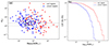 |
Fig. 21. Same as Fig. 17, but for “outflow clumps” and “non-outflow clumps.” |
| In the text | |
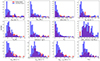 |
Fig. 22. Same as Fig. 18, but for “outflow clumps” and “non-outflow clumps.” |
| In the text | |
Current usage metrics show cumulative count of Article Views (full-text article views including HTML views, PDF and ePub downloads, according to the available data) and Abstracts Views on Vision4Press platform.
Data correspond to usage on the plateform after 2015. The current usage metrics is available 48-96 hours after online publication and is updated daily on week days.
Initial download of the metrics may take a while.