| Issue |
A&A
Volume 693, January 2025
|
|
|---|---|---|
| Article Number | A21 | |
| Number of page(s) | 15 | |
| Section | Interstellar and circumstellar matter | |
| DOI | https://doi.org/10.1051/0004-6361/202450914 | |
| Published online | 23 December 2024 | |
Triggered and dispersed under feedback of super HII region W4
1
Xinjiang Astronomical Observatory, Chinese Academy of Sciences,
830011
Urumqi,
PR China
2
University of Chinese Academy of Sciences,
100080
Beijing,
PR China
3
Key Laboratory of Radio Astronomy, Chinese Academy of Sciences,
830011
Urumqi,
PR China
4
Xinjiang Key Laboratory of Radio Astrophysics,
Urumqi
830011,
PR China
5
Max-Planck-Institut für Radioastronomie,
Auf dem Hügel 69,
53121
Bonn,
Germany
6
Energetic Cosmos Laboratory, Nazarbayev University,
Astana
010000,
Kazakhstan
7
Institute of Experimental and Theoretical Physics, Al-Farabi Kazakh National University,
Almaty
050040,
Kazakhstan
★ Corresponding authors; This email address is being protected from spambots. You need JavaScript enabled to view it.
, This email address is being protected from spambots. You need JavaScript enabled to view it.
, This email address is being protected from spambots. You need JavaScript enabled to view it.
Received:
29
May
2024
Accepted:
13
November
2024
Abstract
The W3/4 Giant Molecular Cloud (GMC) was an ideal target to study the impact of HII regions onto the surrounding molecular gas and star formation. We utilized PMO CO (1−0) data from the Milky Way Imaging Scroll Painting (MWISP) survey to analyze the cloud structure and the feedback effect from the W4 HII region. Our observations showed that cold gas, traced by CO, mainly resided in the W3 GMC, with C18O concentrated in dense regions, while gas around W4 was dispersed. The 13CO position-position-velocity (PPV) distributions revealed a “C” shaped structure in the W3 cloud with more redshifted gas at higher galactic longitudes. A high density layer (HDL) region on the eastern side of the W3 region exhibited a flattened structure facing W4. Subdividing the area into 16 subregions, we found that regions 6–9 on the HDL layer exhibited the strongest radiation, while clouds at the W4 bubble boundary not facing W3 exhibited weak signals, possibly due to star formation triggering and subsequent molecular gas dispersal by the HII region. Analysis along four paths from the W4 HII region to the far side showed a consistent trend of sharply increasing intensity followed by a slow decrease, indicating the gas was effectively eroded and heated by the photon dominated region (PDR) near the boundary of the HII region. Clump identification based on 13CO emission revealed 288 structures categorized as “bubble,” “HDL,” and “quiescent” clumps. Analysis of mass-radius and Virial-mass relationships showed a potential for high-mass star formation in 29.5% (85/288) of the clumps, with 39.2% (113/288) being gravitationally bound. HDL clumps exhibited distinct L/M and velocity dispersion, suggesting an earlier evolutionary stage and gravitational instability compared to quiescent and bubble clumps. Clump parameter differences provided evidence for triggered and dispersed effects of the W4 HII region on the HDL and bubble regions, respectively.
Key words: methods: observational / ISM: clouds / HII regions / ISM: kinematics and dynamics / ISM: structure
© The Authors 2024
 Open Access article, published by EDP Sciences, under the terms of the Creative Commons Attribution License (https://creativecommons.org/licenses/by/4.0), which permits unrestricted use, distribution, and reproduction in any medium, provided the original work is properly cited.
This article is published in open access under the Subscribe to Open model. This email address is being protected from spambots. You need JavaScript enabled to view it. to support open access publication.
1 Introduction
During the evolution of HII regions, massive stars commonly ionize and heat the surrounding gas, while the pressure produced from the high-temperature gas inside the HII region caused the surrounding gas to expand and disperse outwards. This process leads to triggered star formation proceeding through the action of two different mechanisms: by the radiatively driven implosion model (Klein et al. 1980; Bertoldi 1989; Bertoldi & McKee 1990) or the collect-and-collapse mechanism (Elmegreen & Lada 1977; Whitworth et al. 1994). On the other hand, feedback from HII regions could inhibit star formation by clearing away dust and gas (Bisbas et al. 2011; Dale et al. 2013; Walch et al. 2013), especially in lower density clouds. Therefore, star formation could be suppressed in some locations and triggered in others (Dale et al. 2012). For regions far from external feedback, molecular cloud gas primarily underwent spontaneous star formation due to turbulent fragmentation driven by its own gravitational instability (Padoan & Nordlund 2002).
The W3 and W4 giant molecular clouds (hereafter, W3/4), located right on the galactic plane in the Auriga region of the Perseus arm with a distance of about 1.95 kpc, were an archetypal massive star nursery and offered an excellent laboratory to study the different effects of feedback from HII regions (Xu et al. 2006). W4 was a super bubble with a diameter of approximately 40 pc, filled with intense ionizing radiation (Terebey et al. 2003). Normandeau et al. (1997) first conducted high-resolution observations of the W3/W4/W5/HB 3 Galactic complex, focusing on a large field of view in continuum and HI atomic hydrogen. They demonstrated that the most striking feature was a large HI shell encircling the continuum emission. Notably, above the W4 HII region, a conical void appeared in the HI distribution. This structure was subsequently confirmed to be a typical “Galactic chimney” that transports hot gas from the disk to its halo (Normandeau et al. 1996). Taylor et al. (1999) obtained high-resolution images of two compact molecular clouds surrounding the chimney in the CO (2−1) line, proposing that these clouds were driven by ionization fronts generated by the UV radiation from nearby O stars. Lagrois & Joncas (2009a,b) conducted an Hα survey of the W4 HII region (which includes tenuous ionized material) and performed analyses on both the southern and northern parts. They found that the overall kinematics of W4-south were best explained by the Champagne model, which involves at least ten independent gas flows crisscrossing the nebula. Meanwhile, the large-scale trends in radial velocities and line widths in W4-north corresponded to highly accelerated, well-parallelized outflows of vented ionized material, consistent with the expected kinematic signature of the chimney model. These results confirmed that the atomic and molecular gas in the region had been largely cleared out by the OB stars in IC 1805 (Normandeau et al. 1996, 1997). And the impact exerted a stronger influence on W3 and a weaker influence on W5, respectively (Karr & Martin 2003; Oey et al. 2005). The high-density layer (HDL) in W3 east formed the western edge of the W4 super bubble, a structure believed to be triggered by the W4 HII region (Lada et al. 1978; Carpenter et al. 2000; Oey et al. 2005). The HDL represented the most active star formation sites within the W3 molecular cloud, encompassing regions such as W3 Main, W3(OH), and AFGL 333, which were regarded as typical sites of high-mass star formation across various evolutionary stages (such as, Tieftrunk et al. 1995; Normandeau 1999; Rivera-Ingraham et al. 2011, 2013; Bik et al. 2014; Román-Zúñiga et al. 2015; Rivera-Ingraham et al. 2015; Navarete et al. 2019). In contrast to the aforementioned regions, the western portion of W3 is characterized by abundant molecular gas unaffected by external feedback. The HII region KR 140 within it had been suggested to be the result of a rare case of spontaneous high-mass star formation (Ballantyne et al. 2000; Rivera-Ingraham et al. 2011). Unlike the W5 region that consisted of two major HII regions (such as, Shen et al. 2024), the W3/4 region contained just one major extended HII region, apparently only affecting a part of the neighboring W3 cloud. To evaluate this further was the main goal of this paper.
CO and its isotopologues serve as crucial indicators of molecular clouds and provide essential information on their kinematics (such as, Shu et al. 1987; Dame et al. 2001). Heyer & Terebey (1998) analyzed wide-field images of 12CO (1−0) and far-infrared emissions from the W3–W4–W5 giant molecular cloud complex. Their findings demonstrate that the gas component entering the spiral arm was predominantly atomic, with much of the measured far-infrared flux originating from star-forming regions. Yamada et al. (2024) and Polychroni et al. (2010) analyzed the physical characteristics and dynamical properties of the W3 molecular complex using CO (J = 2−1) and CO (J = 3−2) lines, respectively. Li et al. (2019) used Purple Mountain Observatory (PMO) CO (1−0) isotopologue data to identify 459 outflow candidates in a 110 square degree region encompassing the W3/4/5 area. Then they analyzed the feedback effects of these outflows on the parent molecular cloud (Li et al. 2020). Sun et al. (2020), using PMO CO data spanning 110 square degrees, analyzed the large-scale structure and physical properties of the inter- and outer-arms of the Milky Way. Liang et al. (2021) examined the relationship between AFGL 333 and surrounding HII regions using CO data covering a region of 0.05 square degrees. For denser structures, Keown et al. (2019) used Green Bank Telescope (GBT) NH3 data to analyze the relationship between clump structures and filaments in 11 molecular clouds, including the W3 molecular cloud. Rivera-Ingraham et al. (2013, 2015) analyzed the high-mass star formation activity across the entire W3 cloud using Herschel data from the key program HOBYS (Herschel imaging survey of OB young stellar objects). Most studies have focused primarily on the large-scale structure of the W3 molecular cloud and the high-mass star formation activity within the HDL. In contrast, our study focuses on the different feedback effects of the W4 HII region on the molecular gas distribution and star formation activity in entire W3/4 region at a large scale.
In this article, we mainly use the three CO (1−0) isotopologues obtained at the Purple Mountain Observatory (PMO) 13.7 m single dish telescope to analyze the influence of the W4 super-HII region on the molecular distribution and the star formation. The article is organized as follows: in Sect. 2, we introduce our CO observations and data reduction. The overall distributions of CO in 16 sub-regions and in position–position–velocity (P–P–V) space are highlighted in Sect. 3. In Sect. 4, we analyzed the trigger and disperse effect of the W4 super HII region on the surrounding molecular gas and the evolutionary state of the clumps. Our main conclusions are summarized in Sect. 5.
2 Observations
We performed maps of a 3.25° × 1.76° area centered at galactic coordinates 1=134.125°, b=0.81°, covering the W3/4 molecular clouds (5.725 deg2), which was part of the dataset (110 deg2) discussed in Li et al. (2019, 2020) and Sun et al. (2020). This mapping utilized data from the Milky Way Imaging Scroll Painting (MWISP) project, a comprehensive survey in 12CO/13CO/C18O (J = 1−0) across the northern galactic plane. The MWISP project, led by the Purple Mountain Observatory (PMO), aimed to map CO and its isotopic transitions across the accessible galactic plane (Su et al. 2019). Observations were conducted using PMO’s 13.7 m telescope equipped with a nine-beam superconducting spectroscopic array receiver. This setup, operating in sideband separation mode and employing a fast Fourier transform spectrometer (Shan et al. 2012), allowed simultaneous observation of three CO isotopologues (12CO, 13CO, and C18O).
The 12CO line was observed in the upper sideband with a half-power beamwidth (HPBW) of 49″, while the 13CO and C18O lines were observed in the lower sideband with an HPBW of 51″. The data were gridded to 30″ pixels for all three transitions. Bandwidths of 1000MHz were obtained with 16384 channels resulting in channel separations of approximately 0.16 km s−1 for 12CO and 0.17 km s−1 for 13CO and C18O. The typical RMS noise levels of the spectra were 0.25 K for12CO and 0.14 K for both 13CO and C18O. The mean signal-to-noise ratios (SNR) for 12CO, 13CO, and C18O were 23.6, 16.1, and 6.4, respectively. System temperatures were typically 280 K for 12CO and 185 K for 13CO and C18O. The telescope’s pointing accuracy was better than 5″. Mapping observations employed the on-the-fly (OTF) mode with a constant integration time of 14 seconds per point, a scan speed of 50″ s−1, and a step of 15″. The final data, recorded on a main beam brightness temperature scale (Tmb), underwent reduction using Astropy1. For further details on observations and data reduction strategies, please refer to Xu et al. (2006), Li et al. (2019, 2020) and Sun et al. (2020).
3 Results
3.1 CO integrated properties
The molecular W3/4 complex is part of the Perseus Arm and the Local Standard of Rest (LSR) velocity range is limited by −63 and −30 K km s−1 (Sun et al. 2021). Fig. 1 presents 13CO velocity-integrated intensity contour lines superimposed on the W3/4 optical image. This result shows the cold molecular gas is mainly distributed in the W3 molecular cloud region and appears as an enclosing ring. In the W4 HII region, less molecular gas is retained due to strong stellar radiation feedback. 12CO emission is distributed at the boundaries of the bubble. At the junction of W3 and W4, there are three fragments of long (~36 pc), narrow (~6 pc) high-density layers (HDLs) (Lada et al. 1978), corresponding to AFGL333, W3(OH) and W3 Main, respectively.
Fig. 2a shows moment 0 maps of the three CO J = 1−0 emission lines. The background grey image, black contour line, and pink intensity map correspond to 12CO, 13CO, and C18O velocity-integrated intensity, respectively. The three emission lines are mainly distributed over the W3 molecular cloud while no emission is seen inside and only weak emission is seen around the W4 region with the exception of its high galactic longitude side. On the other hand, C18O is mainly distributed in the densest part of the W3 molecular cloud, and almost all of the emission is filament-shaped. Based on their intensity distribution, we divided the molecular complex into 16 subregions and marked them with white dot boxes and corresponding serial numbers. Regions 1–5 are all located on the W4 HII region boundaries, regions 6–9 are located on the HDL, while regions 10–16 are located in more quiescent regions of W3. Notably, although the HDL is believed to be influenced by the expansion of the W4 HII region, the CO contour line shows that only region 6 (AFGL 333) was being significantly eroded by the UV flux from the W4 O stars. In contrast, W3 Main and W3(OH) appear to have been more strongly influenced by the IC 1795 cluster.
In Fig. 2b, we show the average spectra intensity weighted averages within the individual regions with the black, blue, and red line corresponding to 12CO, 13CO, and C18O, respectively. The average spectra in each region were obtained from the spectra of all pixels with a signal-to-noise ratio greater than 3. The spectra show that regions 1–5 on the W4 HII region boundary had the lowest CO radiation intensity and regions 6–9 on the HDL had the highest intensity. The spectra in each sub-region also show a different velocity range. From the velocity values corresponding to the average spectra, only 12CO emissions in regions 2 and 3 exhibited multiple velocity components, while the average spectra for the other regions displayed a single velocity. Another significant feature is that Region 7 was more kinematically connected to Regions 8 and 15. If we assume that Regions 7 and 15 were completely unaffected by external feedback, the velocity offset observed in Region 6 was likely due to the expansion of the W4 HII region. The analysis of two velocities observed by Liang et al. (2021) in the AFGL333 Ridge supports this conclusion. Regions 8 and 9 were situated around the star cluster IC 1795. Normandeau (1999) observed HI spectra in the W3 HII region and suggested that the overall shape of the spectra aligns with predictions from the Two-Arm Spiral Shock model. However, our average spectra indicate that the CO emissions in these two regions were moving away from each other. Although the star formation activity in this area was believed to be influenced by the feedback from the W4 HII region, it now seemed predominantly governed by the W3 HII region at the centers of the two areas. Region 1 was kinematically close to the HDL and shares the same velocity as Region 7, while Regions 2–5 were kinematically distinct from the HDL. Normandeau et al. (1996) observed HI in Region 5 and identified the striking arrow-shaped cloud as a typical example of galactic chimneys. Subsequently, Taylor et al. (1999) conducted a CO velocity gradient analysis and a star cluster age comparison in this area, concluding that the cloud was driven by an ionization front caused by the UV radiation from a nearby O star. Lagrois & Joncas (2009a,b) observed Hα in W4 and noted that the gas flow patterns in the northern and southern parts of the W4 HII region correspond to the chimney and champagne models, respectively. The varied velocity values observed in Regions 1 to 5 might have been related to the two modes of motion generated by the feedback from the W4 HII region.
 |
Fig. 1 Optical Digitized Sky Survey (DSS) red–green–blue (RGB) image (Red: DSS2 Red (F+R); Blue: DSS2 Blue (XJ+S); Green: DSS2 NIR (XI+IS).) of the W3/4 region. Color contours are velocity-integrated intensity of 13CO (1−0) emission in the integrated Local Standard of Rest velocity range from −63 to −28 km s−1, starting at 10 K km s−1 (3σ with light blue) on a main beam brightness temperature scale and go up in steps of 15 K km s−1 (more and more red). White stars and black plus signs indicate identified OB stars (Roman-Lopes et al. 2019) and high-mass young stellar object (HMYSOs) (Lumsden et al. 2013), respectively. Since the W3/4 complex is located near the northern tip of the galactic plane within the equatorial coordinate system, galactic longitude and latitude are approximately parallel to right ascension and declination, so that the terms north, south, east and west are almost synonymous in both coordinate systems and are applied below sometimes without explicitly mentioning the reference system. |
 |
Fig. 2 12CO (1−0) moment 0 map and average spectra of sixteen sub-regions for the W3/4 region. (a) 12CO (1−0) moment 0 (velocity integrated intensity) map of the W3/4 region. The integrated Local Standard of Rest velocity range is −63 to −30 km s−1. The black contour line is the 13CO intensity in the integrated Local Standard of Rest velocity range from −63 to −28 km s−1, starting at 10 K km s−1 (3σ) on a main beam brightness temperature scale and going up in steps of 15 K km s−1. The red areas refer to positions with notable C18O emission. Sixteen dotted boxes mark the dense areas in the whole W3/4 region. The yellow stars and red crosses correspond to OB stars (Roman-Lopes et al. 2019) and high-mass young stellar objects (HMYSOs) (Lumsden et al. 2013), respectively. (b) Average spectra of the sixteen sub-regions for the 12CO (black), 13CO (blue) and C18O (red) J = 1−0 emission lines. The yellow dotted line in each sub-region marks the velocity value corresponding to the peak of the 12CO average spectrum. The upper left corner of each sub-map shows the corresponding sub-region given in (a). |
 |
Fig. 3 (a) PPV (position–position–velocity) Tmb intensity map of 13CO emission in W3/4. (b) PPV velocity map (the velocity at the Tmb peak in each voxel) of 13CO in W3/4. The intensity map on the background panel corresponds to the Tmb projection of the PPV map in that direction. A C-shaped morphology of the gas is revealed by the left panel at lower galactic longitudes. |
3.2 PPV distribution
Fig. 3 presents position-position-velocity (PPV) maps of 13CO J=1−0 in the W3/4 molecular cloud complex. To visualize the intensity distribution of CO emission, we select 13CO emission lines to better highlight the distribution of high column density molecular clouds because 12CO is more diffuse than 13CO and C18O is only detected in very small areas, and 13CO is optically thin making it a better probe of the kinematical behavior. Fig. 3a shows the Tmb values of the CO emission in PPV space, and before the map was formed, we had calculated the RMS (σ) of each spectral line for each pixel point on the position-position (PP) space, and finally only retained lines above the 3σ threshold for the data. Based on the filtered cube data, we also only retained the velocity channel values for spectra above the lower 3σ limit corresponding to each spectral line. The distribution of the Tmb value of the 13CO cube data along longitude, latitude, and velocity axes can be seen on three projection surfaces. The PPV map clearly shows that W3 presents a continuous “C”-shaped halfring gas distribution, while there was less gas on the W4 side. The gas intensity values of the HDL were the highest and were accompanied by a large velocity span, especially in W3 Main, such as, the W3 Main average line range in Fig. 2b was from −48 to −35 km s−1. And from the projection of the Tmb value on the latitude-velocity plane in the PPV space, it could be found that the intensity value of the gas may have had a linear relationship with the latitude axis.
To show the velocity information of the CO gas, Fig. 3b replaces the Tmb value in Fig. 3a with the velocity value corresponding to each voxel. The redshift phenomenon of clouds in the northern region of W3 was clearly more pronounced than that in the southern region. This was evident from the average spectrum lines shown in Fig. 2b. Tchernyshyov et al. (2018) presented detailed gas velocity maps and compared them to the Stationary Density Wave model of the Milky Way spiral structure (Lin & Shu 1964). They suggested only dynamic spiral structure theory (Sellwood & Carlberg 1984; Grand et al. 2012; Baba et al. 2013; D’Onghia et al. 2013)2 can account for the complexity of the Milky Way’s velocity field and the divergence of the velocity field detected in the Perseus arm. Román-Zúñiga et al. (2019) presented evidence of Hubble flow-like motion of young stellar populations away from the Perseus arm. They suggested that the motion of these young stars was related to the divergence of the velocity field3 formed during the evolution of the spiral arms. Therefore, the observed velocity difference of gas between the northern and southern regions in W3 may have been related to this divergence of the velocity field.
To further analyze the distribution of the molecular cloud in the PPV space, we provide six different perspectives in Fig. 4 based on the Tmb value distribution map in Fig. 3a (the azimuth angle of 180° leads to an x-axis parallel to the longitude axis. Rotating clockwise, we chose 150°, 180°, 210°, 240°, 270° and 300° to better visualize the structure of the W3/4 complex). It was evident that the high galactic longitude and low galactic longitude parts of W3, as well as the gas on the HDL layer (W3 Main, W3(OH), and AFGL 333), were separated from each other. There was no apparent direct interaction between these three parts. The gas on the HDL layer facing the W4 HII region exhibited a noticeably flattened morphology, and this shape was consistent with the outer rim of the W4 HII region. This was particularly evident in the subplots with rotation angles of 210 and 240°. Regarding the affected state of the gas on the HDL layer, AFGL 333 showed a significant blueshift, W3 Main represented the region with the most severe redshift in the entire area, and W3(OH) exhibited a slightly weaker blueshift than AFGL333, as also observed in the spectral lines of the subregions in Fig. 2b. On the other hand, the gas on the boundary of the W4 bubble was relatively dispersed, In Normandeau et al. (1996), a comparison was made between the age required for a wind-driven shell in a uniform-density medium and the ages of nine O-type stars in W4. This demonstrated that the stars’ ages were approximately consistent with the time needed for their wind energy to create a chimney, suggesting that the blow-out of the chimney might have been a very recent phenomenon. Outside the chimney region, Lagrois & Joncas (2009a,b) conducted a detailed analysis of the Hα ionized flows in the northern and southern parts of W4. They suggested that these ionized flows, through interactions with molecular gas, led to the erosion of molecular clouds. This was manifested by high-temperature, high-velocity ionized gas impacting the edges of the clouds, thereby accelerating gas loss. This process was typically accompanied by the movement of the ionization front, causing changes in the dynamical characteristics of the molecular gas. For example, the Champagne model indicated that newly ionized material initially retained the kinematics of the eroded material, but was then accelerated by pressure discontinuities, resulting in small-scale Champagne flows. Therefore, the observed diffuse CO gas in the W4 super-bubble may have provided evidence for this erosion process. All these results may have respectively provided evidence for the triggering and dispersing effects of W4 on the gas on the HDL layer and the boundary of the W4 bubble.
 |
Fig. 4 Six different perspectives of the 13CO J = 1−0 PPV-Tmb intensity map described in Fig. 3a. An azimuth angle of 180° leads to an x-axis parallel to the longitude axis. Rotating clockwise, we chose 150°, 180°, 210°, 240°, 270° and 300° to elucidate the structure of the W3/4 complex. The upper right corner of each subgraph shows a schematic representation of the azimuth coordinates in the longitude and latitude planes, and the red dot indicates the angle of view corresponding to the azimuth. The black solid line represents the rotation axis, while the curve above the axis and the red dot depict the trajectory and direction of the rotation axis, respectively. |
4 Discussion
4.1 Effects of feedback on the molecular gas
4.1.1 CO excitation temperature and column density
Under the assumption of optically thick 12CO emission and local thermodynamical equilibrium (LTE; see also Appendix A), the 12CO excitation temperature (Tex) can be estimated (Nagahama et al. 1998; Wilson et al. 2008; Shirley 2015; Liu et al. 2013). Subsequently, assuming the excitation temperatures of 13CO were the same as those of 12CO, the column densities of 13CO (N13) were determined from the velocity-integrated intensities of 13CO (Garden et al. 1991; Pineda et al. 2010). Then, the column densities of 12CO are obtained from N13 using the isotopic ratio of [12C/13C]=75.3 for W3(OH) at a galactocentric distance of 9.64 kpc (Wilson & Rood 1994; Henkel et al. 1994; Yan et al. 2019, 2023). Finally, the H2 column densities were derived by assuming an [H2/12CO] abundance ratio of 1.1 × 10⁴ (Frerking et al. 1982). The distributions of the excitation temperature (Tex) and H2 column density are shown in Fig. 5.
The Tex values in Fig. 5a indicated high Tex primarily located at the boundary regions of the W4 HII region, including the HDL (from 21.6 to 52.1 K with a mean value 26.6±5.1 K) and the W4 super bubble (from 9.7 to 26.0 K with a mean value 13.8±3.1 K). Conversely, the gas located in the western part of the W3 HDL layer exhibited relatively lower temperature values (from 6.5 to 24.1 K with a mean value 10.7±2.6 K). Additionally, the gas situated towards the eastern side of the HDL layer, demonstrated relatively higher Tex values, this phenomenon was more clearly illustrated in the zoomed-in map of Tex at AFGL333 and W3(OH) in Fig. 6. The mean Tex values in the eastern and western parts of W3(OH) were 32.7±5.4 and 28.7±1.5 K, respectively. The mean Tex values in the eastern and western parts of AFGL 333 were 28.6±4.4 and 23.5±1.4 K. Polycyclic aromatic hydrocarbon (PAHs) were known to be closely associated with ionization fronts and photon-dominated regions (PDRs). A comparison of the distributions of PAHs, represented by the 8 µm emission, and Tex revealed a nearly identical pattern: regions with stronger PAH emission also exhibited higher excitation temperatures. However, when examining the column density, it was noted that the gas column density in these high Tex regions was lower than that in areas with weaker PAH emission. At the boundary of the W4 HII region, the strong correlation between PAHs and excitation temperature (Tex) indicated significant radiative heating from the ionization front. Nonetheless, the lower gas column density in these high Tex regions reflected the erosion of neutral material by the ionized gas. The heating and gas expansion induced by the ionization front lead to the dilution of neutral molecules and materials, particularly in the dense layers of HDL at the interface between the W4 HII region and the W3 molecular cloud, further emphasizing the erosive effect of the ionized gas on the surrounding molecular clouds (Lagrois & Joncas 2009a,b).
Furthermore, the H2 column density in Fig. 5b also indicated higher column densities in the HDL (from 1.5×10²² to 2.1×1023 cm−2 with a mean value 3.3±2.2×1022 cm−2), while the gas located at the boundary of W4 appeared to be largely dispersed and exhibited column density values almost equivalent to those of the gas in W3 west (from 1.0×10²¹ to 2.5×1022 cm−2 with a mean value 3.5±3.1×1021 cm−2). Although minor differences existed between our Tex and H2 column density values with those of previous studies such as Keown et al. (2019) for NH3, Rivera-Ingraham et al. (2013) for Herschel dust, and Polychroni et al. (2012) for CO(3−2) regarding the calculations for the W3 molecular cloud, the overall distribution trends are consistent. The discrepancies could be attributed to CO (1−0) representing primarily lower density gas. These observations supported the notion that pressure from the expanding HII region and stellar winds around the exciting stars of W4 likely caused the observed high-density layer at the edge of the W3 molecular cloud to be swept up, as well as the rarefied gas along the other boundaries of W4.
 |
Fig. 5 Maps of (a) CO excitation temperature distributions and (b) H2 column density distribution traced by 13CO. The black contour line corresponds to the intensity of the 8 µm flux starting at 1.3 × 10⁻⁶ W/(m−2 sr) and going up in steps of 5 × 10⁻⁶ W/(m−2 sr). The four red lines are the intercepted paths for the four parameter (12CO intensity, H2 column density, Tex, and 8 µm flux) value distributions in the Fig. 7, and the red numbers indicate the starting position of each path. The yellow stars and black crosses are same as Fig. 2. |
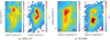 |
Fig. 6 Zoom in map of CO excitation temperature and H2 column density distribution at AFGL 333 and W3(OH) region. Black contour lines are same as Fig. 5. |
4.1.2 Gas compressed and dispersed under feedback
The Tex and  values in Sect. 4.1.1 revealed distinct environmental properties for the high-density layer (HDL), the quiescent region in W3 west, and the boundary shell of the W4 HII region. The HDL layer was situated at the boundary of the W4 super HII region and displayed the strongest CO and PAH emission in the entire region. Lada et al. (1978) and Thronson et al. (1980) suggested that the HDL had experienced strong feedback from W4 HII region, indicating enhanced star-forming activity and the presence of massive stars. The molecular gas distribution at the W4 HII region boundary showed the weakest characteristics. Lagrois & Joncas (2009a,b) analyzed Hα and proposed that an ionized flow resembling Champagne flows is eroding the gas in the boundary shell of the W4 HII region. Conversely, Normandeau et al. (1997) and Routledge et al. (1991) used continuum observations at 1420 MHz and 408 MHz, respectively, to clearly show the shell in the neighboring W3, arguing that the HB3 supernova remnant was interacting with the W3 molecular cloud. However, given that the column density, excitation temperature, and PAH emission in the northern and southern regions of W3 West were nearly identical, we believed that the influence of HB3 on W3 West could be considered negligible compared to the ionization erosion effects of the W4 HII region. Thus, W3 West served as an ideal area for spontaneous star formation. Based on these features, we classified the molecular cloud into three parts: “bubble,” “HDL,” and “quiescent” region, corresponding to the subregions “A,” “B,” and “C” labeled in Fig. 5.
To analyze the feedback region of the W4 HII region on the surrounding molecular gas, we employed the Midcourse Space Experiment (MSX) 8.28 µm flux as a tracer for feedback, as suggested by Mazumdar et al. (2021). This flux represented the intensity at mid-infrared wavelengths resulting from the re-excitation of far-ultraviolet (FUV) radiation from hot stars absorbed by polycyclic aromatic hydrocarbons (PAHs) (Allamandola et al. 1989; Rathborne et al. 2002; Tielens 2008). The black contour lines in Fig. 5 corresponded to the MSX 8.28 µm flux. It is evident that the 8.28 µm flux was predominantly distributed in the HDL and bubble regions, as well as in the spontaneous star-forming region KR 140 within the quiescent region. Conversely, subregions 2 and 3 labeled in white boxes exhibited minimal 8.28 µm flux distribution. This may have be related to the distance from the center of the HII region and the density of the gas. PAHs were closely associated with ionization fronts (that is, photon-dominated regions, or PDRs). Within the W4 HII region, ionized gas filled the space and had evolved over 3.7–4.3 Myr to form a superbubble approximately 40 pc in diameter (Terebey et al. 2003), with the molecular and atomic material at the boundary largely eroded by ionization and photodissociation processes (Lagrois & Joncas 2009a,b). In the HDL layer, where gas density is relatively high, a significant accumulation of ionized gas occured, which may have limited the erosion of molecules farther away. Consequently, the HDL layer exhibited strong PAH signals and higher excitation temperatures. Additionally, its proximity to the central star cluster of W4 further supported the idea of accumulation of ionized gas in this region.
Additionally, to analyze the effect of the W4 HII region on the surrounding gas distribution, we extracted distribution profiles of 12CO integrated intensity, H2 column density, excitation temperature (Tex), and 8 µm flux along four paths marked by red lines in Fig. 5, extending from the side near the center of the W4 HII region to the opposite side. Before plotting the profiles, the 8 µm map was smoothed to the same resolution as the other CO maps, that is, to 30″. Fig. 7 depicted the distribution profiles of the four parameters along four different arbitrarily selected directions leading away from the center. Profiles 1, 2, and 3 all showed a sharp increase on the side facing the center of W4, followed by a steady decrease as we moved away from the center, indicating significant enhancement of these values at the leading edge compared to the trailing edge. These results suggested that the gas was heated on the leading edge of the molecular cloud facing the central cavity, and a higher pressure at the cloud surfaces led to the front end of the cloud acting as a shield for the rest of the gas trailing it, demonstrating that the PDR effectively shielded the molecular cloud by absorbing the bulk of the FUV photons. For profile 4, only H2 column density and Tex exhibited a sharp increase on the side facing the center of W4, which also indicated the shielding effect of the molecular gas front on feedback. However, due to the lower column density in this region, radiation propagated further away, which was confirmed by the distribution profile of the 8 µm flux. Overall, gas located in the bubble region exhibited lower density, temperature, and 8 µm flux values compared to the compressed HDL region, demonstrating a noticeable dispersed trend.
4.2 Effects of feedback on clumps
4.2.1 Identify 13CO clumps
Clumpy structures with fractal and turbulent properties in giant molecular clouds are often referred to as clumps or cores (Blitz 1987), which represent the initial state of star formation. Typically only those with masses larger than 300–500 M⊙ were gravitationally bound and produced stars; those below 300 M⊙ were not bound (Blitz 1991). At the same time, they were highly susceptible to external environmental feedback, especially radiation from massive stars, which promoted or inhibited star-forming activity in the clump. Therefore, analyzing the clumps will helped us gain a deeper understanding of the impact from the expansion of the W4 ionized gas and radiation from the W4 stars on star formation activities.
Dendrograms4 are a proven identification method that excels at identifying clumpy features in both continuum (Kirk et al. 2013; Könyves et al. 2015) and molecular line-emission observations (Rosolowsky et al. 2008; Goodman et al. 2009; Seo et al. 2015; Friesen et al. 2017; Keown et al. 2017). We employed the astrodendro algorithm to identify the leaves structure as clumps in the 13CO position-position-velocity (ppv) space. For the dendrogram algorithm input parameters, we selected min_value = 3×rms, min_delta = 3×rms, and min_npix = 18 pixels (with a pixel size of 30″). Following the methodology outlined by Rosolowsky & Leroy (2006); Rosolowsky et al. (2008) and Shen et al. (2024), we generated the clump catalog and associated properties. A total of 288 clump structures were identified, and all the clump properties were described in Appendix B. Based on the distinction of the W3/4 molecular clouds in Sect. 4.1.2, we classified clumps as “Bubbles” (21.9%, 63/288), “HDL” (23.2%, 67/288), and “quiescent” clumps (54.9%, 158/288), corresponding to the green, red, and blue contours in Fig. 8, respectively.
 |
Fig. 7 12CO intensity, H2 column density (proportional to N13, see Eq. (A.3) in Appendix A), excitation temperature Tex, and 8 µm flux profile along four path described in Fig. 5. |
4.2.2 Clumps triggered and dispersed under feedback
To analyze the capability of clumps to form high-mass stars and compare the differences among the three clump categories mentioned above, we presented in Fig. 9 the mass-radius relationships, Virial-mass relationships, and cumulative distribution functions (CDF) of these clumps. In the figures, green, red, and blue correspond to bubble, HDL, and quiescent clumps, respectively. In Fig. 9a, the mass-radius relationship indicated that only 29.5% (85/288) of the clumps lay above the threshold for high-mass star formation, as denoted by the black dashed line (Kauffmann & Pillai 2010). Among these, HDL clumps exhibited 44.8% (30/67) above the threshold, while Bubble clumps showed a mere 11.1% (7/63), and quiescent clumps had a 30.4% (48/158) capability of forming high-mass stars. Fig. 9b illustrated the observed mass versus virial parameter for all clumps. Among all observations, 39.2% (113/288) fell below the αvir = 2 threshold, indicating gravitational binding, with the majority belonging to quiescent and HDL clumps. Conversely, Bubble clumps predominantly existed in a non-gravitationally bound state, likely influenced by the dispersal effect of the W4 HII region feedback. Fig. 9c displayed the cumulative distribution function (CDF) of clump masses for three distinct regions. Notably, HDL clumps exhibited a flatter CDF compared to the other regions, while Bubble clumps demonstrated a lower trend than quiescent clumps, representative of spontaneous star-forming regions. The slopes of the mass CDFs for the three types of clumps were −0.73±0.03 (bubble), −0.61±0.03 (HDL), and −0.72±0.03 (quiescent). Compared to the slope of the mass function dN/dM discussed by Heyer & Terebey (1998) (−1.73±0.10), the mass distributions in the bubble and quiescent regions were quite consistent with their findings, adhering to a power-law distribution. In contrast, the lower slope in the HDL region indicated that as mass increased, the cumulative distribution of clumps decreased more gradually, suggesting that a majority of the clumps possessed larger masses. These findings collectively corroborated the triggering and dispersal effects of the W4 HII region on the surrounding star formation activity.
To further analyze the influence of W4 feedback on the internal star formation activity within clumps, we presented in Fig. 10 the comparative histogram distributions of all parameters for the three clump categories. It was evident that the three clump categories exhibited distinct distribution patterns. HDL clumps, compared to the other two categories, generally displayed higher excitation temperatures, lower Virial parameters, higher thermal velocity dispersion, and lower L/M (luminosity/Mass) ratios. These were good indicators of their evolutionary stage in star formation (Molinari et al. 2008; Urquhart et al. 2018). On the other hand, bubble clumps exhibited lower excitation temperatures, higher Virial values, higher L/M ratios, lower thermal velocity dispersions, and nearly equivalent non-thermal velocity dispersions as HDL clumps. Both bubble and HDL clumps demonstrated strong non-thermal velocity dispersions, possibly due to the comparable feedback effects experienced by all clumps near the boundary of the W4 HII region. The thermal velocity dispersion of HDL clumps, influenced by internal stellar radiation and gravity, contrasted with the dispersion revealed by the bubble clumps, which resulted in weakened star formation activity under the influence of the HII region. The Lbol/Mclump ratios obtained from the far-infrared and the 13CO column densities represented the evolutionary stage of the individual objects (Urquhart et al. 2018). Latest stages with HII regions were characterized by highest L/M ratios. This was consistent with the fact that the W4 clouds showed the highest L/M ratios, supporting evidence for dispersal activities of the moleclar gas surrounding the W4 region. A Kolmogorov–Smirnov (KS) test (Kolmogorov 1933; Smirnov 1939) was performed on these parameters for each type of clump to assess the conclusion that these three types of clumps corresponded to different evolutionary states. The comparison revealed that only the bubble clumps versus HDL clumps showed large P values (0.49) for the parameters Vrms and σNon–Ther, while the P values for the other parameter comparisons were almost all below 0.03. This supported our view that star formation activity at the boundary of the W4 HII region was dispersed and triggered in the HDL layer.
 |
Fig. 8 Distribution of bubble clumps (green contours), HDL clumps (red contours) and quiescent clumps (blue contours) classified according to their position distribution relative to the super bubble W4. The gray background image represents the integrated intensity map of 13CO. The yellow stars, black crosses, and small red and blue dots correspond to OB stars (Roman-Lopes et al. 2019), HMYSOs (Lumsden et al. 2013) and red and blue lobes identified as CO outflows by Li et al. (2019), respectively. |
 |
Fig. 9 Mass versus radius, Virial versus mass, and Cumulative distribution function (CDF) of mass relation for three type clumps. (a) Mass and radius relationships for all identified 13CO leaves. The red, green, and blue dots correspond to HDL, bubble, and quiescent clumps, respectively (see Fig. 8). The dotted lines shows the best power-law fit to each of the data. The yellow area denotes the empirically derived parameter set m(r) < 870 M⊙(r/pc)1.33, where massive star formation should not occur (Kauffmann & Pillai 2010). (b) Virial and mass relationships for all 13CO clumps, The black dashed lines correspond to positions with virial values of 1 and 2. Values below unity represent the gravitationally bound state and values above two are gravitational unbound,respectively. (c) CDF ofmass between HDL(red line),bubble (green line),and quiescent regions (blue line). The grey dots with errorbars in (a) and (b) show the median mass, radius, and virial parameter uncertainties in different bins along each axis. |
 |
Fig. 10 Comparison of clump parameters of bubbles (green), HDLs (red) and quiescent clumps (blue) in the W3/4 complex. The solid lines overlaid in matching colors show the kernel density estimate (KDE) of the distribution of the corresponding properties. |
5 Summary
Using 12CO/13CO/C18O data from the ongoing MWISP project, we reported a study of the W3/4 complex, including a detailed analysis of large-scale distributions, and the effect of W4 HII region feedback on molecular clouds and clump evolution. The main results were summarized as follows:
Based on the distribution of three CO lines, we observed that CO-traced cold gas mainly resided in the W3 giant molecular cloud, while the gas surrounding W4 was mostly dispersed, with C18O primarily concentrated in the dense regions of W3. According to the PPV spatial distribution map of 13CO, the W3 molecular cloud exhibited a “C” shaped distribution, with more redshifted gas at higher galactic longitudes;
Dividing the entire W3/4 region into sixteen subregions and analyzing the average spectral line distribution of the three CO lines, we found that regions 6, 7, 8, and 9, located on the HDL, exhibited the strongest radiation in the entire region. Gas in quiescent regions showed different velocity distributions at higher and lower galactic longitudes. Clouds located on the boundary of the W4 bubble displayed the weakest signals, with regions 2 and 3 showing multiple velocity components, possibly due to the dispersal effect of the W4 HII region;
By extracting the intensity distributions of 12CO, H2 column density, excitation temperature Tex, and the intensity of the 8 µm continuum, which traced feedback, along four arbitrarily chosen paths from near the center of the W4 HII region to the far side, we observed a consistent trend of a sharp increase at the boundary followed by a gradual decrease. This indicated that gas facing the W4 HII region center was effectively eroded and heated by the photodissociation region (PDR) through the absorption of FUV photons;
Clump identification based on 13CO emission revealed 288 clump structures, categorized as “bubble,” “HDL,” and “quiescent” clumps based on their distribution relative to the W4 HII region. Analysis of the mass-radius relationship and Virial-mass relationship showed that 29.5% (85/288) of the clumps had the potential to form high-mass stars, with 39.2% (113/288) of the clumps being gravitationally bound. Combining the cumulative distribution function (CDF), the three types of clumps exhibited distinct distributions, ranked from strong to weak CO emitters as HDL, quiescent, and bubble clumps’
Histogram distributions of all parameters for the three types of clumps showed significant differences. HDL clumps generally exhibited higher excitation temperatures, lower Virial parameters, higher thermal velocity dispersion, and lower L/M compared to the other two categories. The velocity dispersion distribution indicated that HDL and bubble clumps had similar non-thermal velocity dispersions, while bubble clumps showed the weakest thermal velocity dispersion. Combined Virial and L/M distributions suggested that HDL clumps were in an earlier stage, followed by the quiescent clumps, while bubble clumps are represented a later stage of evolution.
Considering the quiescent region as spontaneous star formation, the above results provided ample evidence for the triggering and dispersing effects of the W4 HII region on the HDL and bubble regions, respectively.
Data availability
Full clump properties are available at the CDS via anonymous ftp to cdsarc.cds.unistra.fr (130.79.128.5) or via https://cdsarc.cds.unistra.fr/viz-bin/cat/J/A+A/693/A21.
Acknowledgements
We like to thank the anonymous referee for the useful suggestions that improved this study. This work was mainly funded by the National Key R&D Program of China under grant No. 2022YFA1603103. It was also partially funded by the Regional Collaborative Innovation Project of Xinjiang Uyghur Autonomous Region under grant no. 2022E01050, the National Natural Science Foundation of China (NSFC) under grants nos. 12173075, 12373029, 12103082, and 12403033, the Tianshan Talent Program of Xinjiang Uygur Autonomous Region under grant No. 2022TSYCLJ0005, Tianchi Talents Program of Xinjiang Uygur Autonomous Region, the Natural Science Foundation of Xinjiang Uygur Autonomous Region under grant no. 2022D01E06, the Chinese Academy of Sciences (CAS) “Light of West China” Program under grants nos. xbzg-zdsys-202212, 2020-XBQNXZ-017, and 2021-XBQNXZ-028, the National Key R&D Program of China with grant 2023YFA1608002, and the Xinjiang Key Laboratory of Radio Astrophysics under grant no. 2022D04033. D.L. acknowledges support from Youth Innovation Promotion Association CAS. C.H. has been funded by the Chinese Academy of Sciences President’s International Fellowship initiative by grant Nos. 2023VMA0031 and 2025PVA0048. Moreover, this work is partially funded by the Science Committee of the Ministry of Science and Higher Education of the Republic of Kazakhstan grant no. AP13067768. This study uses the data from the Galaxy Picture Survey Project. MWISP is sponsored by the National Key R&D Program of China with grant 2023YFA1608000 and the CAS Key Research Program of Frontier Sciences with grant QYZDJ-SSW-SLH047. The Purple Mountain Observatory 13.7 m telescope is used to carry out the north galactic plane 12CO/13CO/C18O multispectral line survey. Thanks to the long-term work of the working group, especially the staff of the Qinghai Observation Station.
Appendix A H2 column density and CO excitation temperature
The H2 column densities were derived using the isotopic ratios of [12C/13C]=75.3, (Wilson & Rood 1994; Henkel et al. 1994; Yan et al. 2019, 2023) for a W3(OH) galactocentric distance of 9.64 kpc, and an [H2/12CO] abundance ratio of 1.1 × 10⁴ (Frerking et al. 1982). For a given cloud, the 12C/13C isotope ratio from H2CO gives an upper limit and the ratio from CO provides a lower limit to the actual ratio (Langer et al. 1984; Tang et al. 2019).
Assuming local thermal equilibrium and that 12CO emission is optically thick (Wilson et al. 2008; Shirley 2015), we use the 13CO J = 1−0 emission to determine the column density and mass of the W3/4 region. Using the method for correcting effects of optical depth by Henkel et al. (1980, 1982, 1983, 1985), we obtain median and mean values for the 12CO/13CO integrated intensity ratio of 6.9 and 8.7, which are significantly smaller than the isotope ratio 12C/13C of 75±4 (Yan et al. 2023). Thus12 CO must be optically thick. Based on these assumptions, the CO excitation temperature (Tex) can be estimated by (Nagahama et al. 1998)
![Mathematical equation: ${T_{{\rm{ex}}}}[{\rm{K}}] = {{5.53} \over {\ln \left( {1 + {{5.53} \over {{{\rm{T}}_{{\rm{MB}},12}}}}} \right)}},$](/articles/aa/full_html/2025/01/aa50914-24/aa50914-24-eq2.png) (A.1)
(A.1)
where TMB,12 is the peak main-beam brightness temperature of 12CO.
We further assume that the excitation temperature of 13CO is equal to the excitation temperature of 12CO. The optical depth of 13CO(τ13) was estimated as (Kawamura & Masson 1998; Pineda et al. 2010):
![Mathematical equation: ${\tau _{13}} = - ln\left[ {1 - {{{T_{{\rm{MB}},13}}} \over {5.29}}{{\left[ {{{\left( {{e^{5.29/{T_{{\rm{ex}}}}}} - 1} \right)}^{ - 1}} - 0.164} \right]}^{ - 1}}} \right],$](/articles/aa/full_html/2025/01/aa50914-24/aa50914-24-eq3.png) (A.2)
(A.2)
where TMB,13 is the peak main-beam brightness temperature of 13CO. The column densities of 13CO can be estimated by the following equations (Garden et al. 1991):
![Mathematical equation: ${N_{13}}\left[ {{\rm{c}}{{\rm{m}}^{ - 2}}} \right] = 2.42 \times {10^{14}}{{\rm{I}}_{13}}.$](/articles/aa/full_html/2025/01/aa50914-24/aa50914-24-eq4.png) (A.3)
(A.3)
Here I13 is a measure of the total integrated intensity of 13CO. It can be estimated as:
![Mathematical equation: ${I_{13}}\left[ {{\rm{Kkm}}{{\rm{s}}^{ - 1}}} \right] = {{{\tau _{13}}} \over {1 - {{\rm{e}}^{ - {\tau _{13}}}}}} \times {{1 + 0.88/{{\rm{T}}_{{\rm{ex}}}}} \over {1 - {{\rm{e}}^{ - 5.29/{T_{{\rm{ex}}}}}}}}\mathop \smallint \nolimits^ {{\rm{T}}_{{\rm{MB}},13}}{\rm{dv}}.$](/articles/aa/full_html/2025/01/aa50914-24/aa50914-24-eq5.png) (A.4)
(A.4)
 |
Fig. A.1 Velocity channel maps of 12CO(1−0) toward W3/4 complex. The emission has been integrated over 3.3 km s−1 around the local standard of rest velocities indicated in each panel. Note: the intensity of each detected and displayed pixel is greater than 3σ. For the yellow stars and small green and red dots, see Fig. 2a. |
 |
Fig. A.2 Velocity channel maps of 13CO(1−0) toward W3/4 complex. |
 |
Fig. A.3 Velocity channel maps of C18O(1−0) toward W3/4 complex. |
Appendix B Catalog of clump properties
After running the dendrogram algorithm on the data cube, a catalog of properties of all the structures can be created with “leaves” representing the smallest structures. We extracted the leave’s morphology from the obtained parameters and treated the leaves as clump structures that could lead to new star formation. The catalog gives information such as the location, mean velocity, total fluxes within the structure, and radius of each leaf on the position-position plane (Rosolowsky & Leroy 2006). Other parameters such as luminosity, virial parameter and thermal velocity dispersion of the clumps are calculated according to the following equations (from eq. B.1 to eq. B.9). All properties of the 288 clumps of 13CO (see Fig. 8) are summarized in online CDS Table.
The radius from the algorithm catalog is in arcsec. We use Rpc = Rarcsecd to calculate the physical radius in pc and L = Fd2 to calculate their luminosities, where d = 1.95±0.04×10³ pc is the distance to W3(OH) (Xu et al. 2006), F has units of K km s−1 arcsec2, and L has units of K km s−1 pc2. Rpc, flux and the luminosity of the cloud, LCO (Rosolowsky & Leroy 2006) can be defined as:
![Mathematical equation: $R[{\rm{pc}}] = {{{\rm{R}}[{\rm{arcseconds}}]} \over {3600}}{\pi \over {180}}{\rm{d}}[{\rm{pc}}]$](/articles/aa/full_html/2025/01/aa50914-24/aa50914-24-eq6.png) (B.1)
(B.1)
 (B.2)
(B.2)
![Mathematical equation: $\matrix{ \hfill {{L_{{\rm{CO}}}}\left[ {{\rm{Kkm}}{{\rm{s}}^{ - 1}}{\rm{p}}{{\rm{c}}^2}} \right] = } \cr \hfill {{F_{{\rm{CO}}}}\left[ {{\rm{Kkm}}{{\rm{s}}^{ - 1}}{{{\mathop{\rm arcsec}\nolimits} }^2}} \right]{{({\rm{d}}[{\rm{pc}}])}^2}{{\left( {{\pi \over {180 \times 3600}}} \right)}^2}} \cr } $](/articles/aa/full_html/2025/01/aa50914-24/aa50914-24-eq8.png) (B.3)
(B.3)
If δx and δy are in units of arcseconds, δv in km s−1, and Ti in K, then the resulting flux will have units of K km s−1 arcsec2.
The velocity dispersion σv can be defined from Full Width at Half Maximum (FWHM) ∆V
![Mathematical equation: ${\sigma _{\rm{v}}}\left[ {{\rm{km}}{{\rm{s}}^{ - 1}}} \right] = {\rm{\Delta V}}/\sqrt {8ln(2)} $](/articles/aa/full_html/2025/01/aa50914-24/aa50914-24-eq9.png) (B.4)
(B.4)
The mass of each clump can be determined by summing up the masses of all the pixels within each leaf. The mass for each pixel is computed by
![Mathematical equation: ${M_{{\rm{pixel }}}}\left[ {{{\rm{M}}_ \odot }} \right] = {{\rm{N}}_{{\rm{tot}}}}\left( {^{13}{\rm{CO}}} \right)\left[ {{{\rm{H}}_2}/{{\rm{C}}^{13}}{\rm{O}}} \right]{\mu _{{{\rm{H}}_2}}}{{\rm{m}}_{\rm{H}}}{{\rm{A}}_{{\rm{pixel }}}},$](/articles/aa/full_html/2025/01/aa50914-24/aa50914-24-eq10.png) (B.5)
(B.5)
where  is the mean molecular weight (Brunt 2010), mH = 1.67 × 10⁻²⁴ g is the mass of a hydrogen atom, [H2/13CO] is assumed to be 8.3 × 10⁵ (from isotope ratios in Sect. A), and Apixel is the area of each pixel within the clump.
The volume density and surface mass density of clumps can be given using their mass and radius:
![Mathematical equation: $n\left( {{{\rm{H}}_2}} \right)\left[ {{\rm{c}}{{\rm{m}}^{ - 3}}} \right] = 15.1 \times {{3M} \over {4\pi {R^3}_{{\rm{pc}}}}}$](/articles/aa/full_html/2025/01/aa50914-24/aa50914-24-eq12.png) (B.6)
(B.6)
and
![Mathematical equation: $\mathop \sum \nolimits^ \left[ {{\rm{gc}}{{\rm{m}}^{ - 2}}} \right] = {M \over {\pi R_{{\rm{pc}}}^2}}$](/articles/aa/full_html/2025/01/aa50914-24/aa50914-24-eq13.png) (B.7)
(B.7)
M is in M⊙, Rpc is in pc, n(H2) is in cm−3, and ∑ is in g cm−2. The factor of 15.1 is used to convert the density to appropriate units.
To estimate the virial stability of these clumps, we adopt the virial analysis method described in Mazumdar et al. (2021). The virial parameter is defined as the ratio of the virial mass of a spherically symmetric cloud to its total mass:
 (B.8)
(B.8)
where σv is the velocity dispersion of the clump and G is the gravitational constant (MacLaren et al. 1988). We assume that these clumps follow a spherical density distribution. In the absence of pressure supporting the clump, αvir < 1 means that the clump is gravitationally unstable and collapsing, whereas αvir > 2 suggests that the kinetic energy is higher than the gravitational energy and that the clump is dissipating. A value of αvir between 1 and 2 is interpreted as an approximate equilibrium between the gravitational and kinetic energies.
The luminosity-to-mass ratio (L/M) of clumps is a good indicator of their evolutionary stage in star formation (Molinari et al. 2008; Urquhart et al. 2018).
To determine the dominant broadening mechanisms, we calculate thermal line widths using  in units of km s−1, where k is the Boltzmann constant in units of J/K, m is the mean molecular mass in units of g, and T is the excitation temperature Tex from eq. A.1. The thermal and non-thermal line widths (σTher and σNon–Ther) are defined using the following equations (Myers 1983; Li et al. 2015):
![Mathematical equation: ${\sigma _{{\rm{Ther,g}}}}\left[ {{\rm{km}}{{\rm{s}}^{ - 1}}} \right] = \sqrt {{{kT} \over {\mu {m_{\rm{H}}}}}} ,$](/articles/aa/full_html/2025/01/aa50914-24/aa50914-24-eq16.png) (B.9)
(B.9)
and
![Mathematical equation: ${\sigma _{{\rm{Non - Ther}}}}\left[ {{\rm{km}}{{\rm{s}}^{ - 1}}} \right] = \sqrt {\sigma _{1{\rm{D}}}^2 - \sigma _{{\rm{Ther}}}^2} = \sqrt {{\rm{\Delta }}_{{{\rm{v}}_{13}}}^2/8ln2 - \sigma _{{\rm{Ther}}}^2,} $](/articles/aa/full_html/2025/01/aa50914-24/aa50914-24-eq17.png) (B.10)
(B.10)
where σ1 D is the one-dimensional velocity dispersion in units of km s−1,  is the line width in units of km s−1, k is the Boltzmann constant in units of J/K, µ = 2.4, mH is the mass of a single hydrogen atom in units of g and T is the excitation temperature in units of K.
References
- Allamandola, L. J., Tielens, A. G. G. M., & Barker, J. R. 1989, ApJS, 71, 733 [Google Scholar]
- Baba, J., Saitoh, T. R., & Wada, K. 2013, ApJ, 763, 46 [Google Scholar]
- Ballantyne, D. R., Kerton, C. R., & Martin, P. G. 2000, ApJ, 539, 283 [NASA ADS] [CrossRef] [Google Scholar]
- Bertoldi, F. 1989, ApJ, 346, 735 [Google Scholar]
- Bertoldi, F., & McKee, C. F. 1990, ApJ, 354, 529 [NASA ADS] [CrossRef] [Google Scholar]
- Bik, A., Stolte, A., Gennaro, M., et al. 2014, A&A, 561, A12 [NASA ADS] [CrossRef] [EDP Sciences] [Google Scholar]
- Bisbas, T. G., Wünsch, R., Whitworth, A. P., Hubber, D. A., & Walch, S. 2011, ApJ, 736, 142 [Google Scholar]
- Blitz, L. 1987, in NATO Advanced Study Institute (ASI) Series C, 210, Physical Processes in Interstellar Clouds, eds. G. E. Morfill, & M. Scholer, 35 [Google Scholar]
- Blitz, L. 1991, in NATO Advanced Study Institute (ASI) Series C, 342, The Physics of Star Formation and Early Stellar Evolution, eds. C. J. Lada, & N. D. Kylafis, 3 [Google Scholar]
- Brunt, C. M. 2010, A&A, 513, A67 [NASA ADS] [CrossRef] [EDP Sciences] [Google Scholar]
- Carpenter, J. M., Heyer, M. H., & Snell, R. L. 2000, ApJS, 130, 381 [NASA ADS] [CrossRef] [Google Scholar]
- Dale, J. E., Ercolano, B., & Bonnell, I. A. 2012, MNRAS, 424, 377 [NASA ADS] [CrossRef] [Google Scholar]
- Dale, J. E., Ercolano, B., & Bonnell, I. A. 2013, MNRAS, 430, 234 [Google Scholar]
- Dame, T. M., Hartmann, D., & Thaddeus, P. 2001, ApJ, 547, 792 [Google Scholar]
- D’Onghia, E., Vogelsberger, M., & Hernquist, L. 2013, ApJ, 766, 34 [Google Scholar]
- Elmegreen, B. G., & Lada, C. J. 1977, ApJ, 214, 725 [Google Scholar]
- Frerking, M. A., Langer, W. D., & Wilson, R. W. 1982, ApJ, 262, 590 [Google Scholar]
- Friesen, R. K., Pineda, J. E., co-PIs, et al. 2017, ApJ, 843, 63 [NASA ADS] [CrossRef] [Google Scholar]
- Garden, R. P., Hayashi, M., Gatley, I., Hasegawa, T., & Kaifu, N. 1991, ApJ, 374, 540 [NASA ADS] [CrossRef] [Google Scholar]
- Goodman, A. A., Pineda, J. E., & Schnee, S. L. 2009, ApJ, 692, 91 [Google Scholar]
- Grand, R. J. J., Kawata, D., & Cropper, M. 2012, MNRAS, 421, 1529 [CrossRef] [Google Scholar]
- Henkel, C., Walmsley, C. M., & Wilson, T. L. 1980, A&A, 82, 41 [NASA ADS] [Google Scholar]
- Henkel, C., Wilson, T. L., & Bieging, J. 1982, A&A, 109, 344 [NASA ADS] [Google Scholar]
- Henkel, C., Wilson, T. L., Walmsley, C. M., & Pauls, T. 1983, A&A, 127, 388 [NASA ADS] [Google Scholar]
- Henkel, C., Guesten, R., & Gardner, F. F. 1985, A&A, 143, 148 [Google Scholar]
- Henkel, C., Wilson, T. L., Langer, N., Chin, Y. N., & Mauersberger, R. 1994, in The Structure and Content of Molecular Clouds, 439, eds. T. L. Wilson & K. J. Johnston, 72 [Google Scholar]
- Heyer, M. H., & Terebey, S. 1998, ApJ, 502, 265 [NASA ADS] [CrossRef] [Google Scholar]
- Karr, J. L., & Martin, P. G. 2003, ApJ, 595, 900 [NASA ADS] [CrossRef] [Google Scholar]
- Kauffmann, J., & Pillai, T. 2010, ApJ, 723, L7 [Google Scholar]
- Kawamura, J. H., & Masson, C. R. 1998, ApJ, 509, 270 [NASA ADS] [CrossRef] [Google Scholar]
- Keown, J., Di Francesco, J., Kirk, H., et al. 2017, ApJ, 850, 3 [NASA ADS] [CrossRef] [Google Scholar]
- Keown, J., Di Francesco, J., Rosolowsky, E., et al. 2019, ApJ, 884, 4 [Google Scholar]
- Kirk, J. M., Ward-Thompson, D., Palmeirim, P., et al. 2013, MNRAS, 432, 1424 [Google Scholar]
- Klein, R. I., Sandford, M. T., I., & Whitaker, R. W. 1980, Space Sci. Rev., 27, 275 [Google Scholar]
- Kolmogorov, A. 1933, Inst. Ital. Attuari, Giorn., 4, 83 [Google Scholar]
- Könyves, V., André, P., Men’shchikov, A., et al. 2015, A&A, 584, A91 [Google Scholar]
- Lada, C. J., Elmegreen, B. G., Cong, H. I., & Thaddeus, P. 1978, ApJ, 226, L39 [CrossRef] [Google Scholar]
- Lagrois, D., & Joncas, G. 2009a, ApJ, 691, 1109 [NASA ADS] [CrossRef] [Google Scholar]
- Lagrois, D., & Joncas, G. 2009b, ApJ, 693, 186 [NASA ADS] [CrossRef] [Google Scholar]
- Langer, W. D., Graedel, T. E., Frerking, M. A., & Armentrout, P. B. 1984, ApJ, 277, 581 [Google Scholar]
- Li, Y., Xu, Y., Yang, J., et al. 2015, AJ, 150, 60 [NASA ADS] [CrossRef] [Google Scholar]
- Li, Y., Xu, Y., Sun, Y., et al. 2019, ApJS, 242, 19 [NASA ADS] [CrossRef] [Google Scholar]
- Li, Y., Xu, Y., Sun, Y., & Yang, J. 2020, ApJS, 251, 26 [NASA ADS] [CrossRef] [Google Scholar]
- Liang, X., Xu, J.-L., Xu, Y., & Wang, J.-J. 2021, ApJ, 913, 14 [NASA ADS] [CrossRef] [Google Scholar]
- Lin, C. C., & Shu, F. H. 1964, ApJ, 140, 646 [Google Scholar]
- Liu, T., Wu, Y., & Zhang, H. 2013, ApJ, 775, L2 [NASA ADS] [CrossRef] [Google Scholar]
- Lumsden, S. L., Hoare, M. G., Urquhart, J. S., et al. 2013, ApJS, 208, 11 [Google Scholar]
- MacLaren, I., Richardson, K. M., & Wolfendale, A. W. 1988, ApJ, 333, 821 [NASA ADS] [CrossRef] [Google Scholar]
- Mazumdar, P., Wyrowski, F., Colombo, D., et al. 2021, A&A, 650, A164 [NASA ADS] [CrossRef] [EDP Sciences] [Google Scholar]
- Molinari, S., Pezzuto, S., Cesaroni, R., et al. 2008, A&A, 481, 345 [NASA ADS] [CrossRef] [EDP Sciences] [Google Scholar]
- Myers, P. C. 1983, ApJ, 270, 105 [Google Scholar]
- Nagahama, T., Mizuno, A., Ogawa, H., & Fukui, Y. 1998, AJ, 116, 336 [NASA ADS] [CrossRef] [Google Scholar]
- Navarete, F., Galli, P. A. B., & Damineli, A. 2019, MNRAS, 487, 2771 [NASA ADS] [CrossRef] [Google Scholar]
- Normandeau, M. 1999, AJ, 117, 2440 [NASA ADS] [CrossRef] [Google Scholar]
- Normandeau, M., Taylor, A. R., & Dewdney, P. E. 1996, Nature, 380, 687 [NASA ADS] [CrossRef] [Google Scholar]
- Normandeau, M., Taylor, A. R., & Dewdney, P. E. 1997, ApJS, 108, 279 [NASA ADS] [CrossRef] [Google Scholar]
- Oey, M. S., Watson, A. M., Kern, K., & Walth, G. L. 2005, AJ, 129, 393 [NASA ADS] [CrossRef] [Google Scholar]
- Padoan, P., & Nordlund, Å. 2002, ApJ, 576, 870 [NASA ADS] [CrossRef] [Google Scholar]
- Pineda, J. L., Goldsmith, P. F., Chapman, N., et al. 2010, ApJ, 721, 686 [NASA ADS] [CrossRef] [Google Scholar]
- Polychroni, D., Moore, T. J. T., & Allsopp, J. 2010, in 9th International Conference of the Hellenic Astronomical Society, eds. K. Tsinganos, D. Hatzidimitriou, & T. Matsakos, Astronomical Society of the Pacific Conference Series, 424, 165 [NASA ADS] [Google Scholar]
- Polychroni, D., Moore, T. J. T., & Allsopp, J. 2012, MNRAS, 422, 2992 [NASA ADS] [CrossRef] [Google Scholar]
- Rathborne, J. M., Burton, M. G., Brooks, K. J., et al. 2002, MNRAS, 331, 85 [NASA ADS] [CrossRef] [Google Scholar]
- Rivera-Ingraham, A., Martin, P. G., Polychroni, D., & Moore, T. J. T. 2011, ApJ, 743, 39 [NASA ADS] [CrossRef] [Google Scholar]
- Rivera-Ingraham, A., Martin, P. G., Polychroni, D., et al. 2013, ApJ, 766, 85 [NASA ADS] [CrossRef] [Google Scholar]
- Rivera-Ingraham, A., Martin, P. G., Polychroni, D., et al. 2015, ApJ, 809, 81 [NASA ADS] [CrossRef] [Google Scholar]
- Roman-Lopes, A., Román-Zúñiga, C. G., Tapia, M., et al. 2019, ApJ, 873, 66 [NASA ADS] [CrossRef] [Google Scholar]
- Román-Zúñiga, C. G., Ybarra, J. E., Megías, G. D., et al. 2015, AJ, 150, 80 [CrossRef] [Google Scholar]
- Román-Zúñiga, C. G., Roman-Lopes, A., Tapia, M., Hernandez, J., & Ramírez-Preciado, V. 2019, ApJ, 871, L12 [CrossRef] [Google Scholar]
- Rosolowsky, E., & Leroy, A. 2006, PASP, 118, 590 [NASA ADS] [CrossRef] [Google Scholar]
- Rosolowsky, E. W., Pineda, J. E., Kauffmann, J., & Goodman, A. A. 2008, ApJ, 679, 1338 [Google Scholar]
- Routledge, D., Dewdney, P. E., Landecker, T. L., & Vaneldik, J. F. 1991, A&A, 247, 529 [NASA ADS] [Google Scholar]
- Sellwood, J. A., & Carlberg, R. G. 1984, ApJ, 282, 61 [Google Scholar]
- Seo, Y. M., Shirley, Y. L., Goldsmith, P., et al. 2015, ApJ, 805, 185 [Google Scholar]
- Shan, W., Yang, J., Shi, S., et al. 2012, IEEE Trans. Terahertz Sci. Technol., 2, 593 [Google Scholar]
- Shen, H., Esimbek, J., Henkel, C., et al. 2024, A&A, 689, A140 [NASA ADS] [CrossRef] [EDP Sciences] [Google Scholar]
- Shirley, Y. L. 2015, PASP, 127, 299 [Google Scholar]
- Shu, F. H., Adams, F. C., & Lizano, S. 1987, ARA&A, 25, 23 [Google Scholar]
- Smirnov, N. V. 1939, Bull. Math. Univ. Moscou, 2, 3 [Google Scholar]
- Su, Y., Yang, J., Zhang, S., et al. 2019, ApJS, 240, 9 [Google Scholar]
- Sun, Y., Yang, J., Xu, Y., et al. 2020, ApJS, 246, 7 [NASA ADS] [CrossRef] [Google Scholar]
- Sun, Y., Yang, J., Yan, Q.-Z., et al. 2021, ApJS, 256, 32 [NASA ADS] [CrossRef] [Google Scholar]
- Tang, X. D., Henkel, C., Menten, K. M., et al. 2019, A&A, 629, A6 [NASA ADS] [CrossRef] [EDP Sciences] [Google Scholar]
- Taylor, A. R., Irwin, J. A., Matthews, H. E., & Heyer, M. H. 1999, ApJ, 513, 339 [NASA ADS] [CrossRef] [Google Scholar]
- Tchernyshyov, K., Peek, J. E. G., & Zasowski, G. 2018, AJ, 156, 248 [NASA ADS] [CrossRef] [Google Scholar]
- Terebey, S., Fich, M., Taylor, R., Cao, Y., & Hancock, T. 2003, ApJ, 590, 906 [NASA ADS] [CrossRef] [Google Scholar]
- Thronson, H. A., J., Campbell, M. F., & Hoffmann, W. F. 1980, ApJ, 239, 533 [NASA ADS] [CrossRef] [Google Scholar]
- Tieftrunk, A. R., Wilson, T. L., Steppe, H., et al. 1995, A&A, 303, 901 [NASA ADS] [Google Scholar]
- Tielens, A. G. G. M. 2008, ARA&A, 46, 289 [NASA ADS] [CrossRef] [Google Scholar]
- Urquhart, J. S., König, C., Giannetti, A., et al. 2018, MNRAS, 473, 1059 [Google Scholar]
- Walch, S., Whitworth, A. P., Bisbas, T. G., Wünsch, R., & Hubber, D. A. 2013, MNRAS, 435, 917 [NASA ADS] [CrossRef] [Google Scholar]
- Whitworth, A. P., Bhattal, A. S., Chapman, S. J., Disney, M. J., & Turner, J. A. 1994, A&A, 290, 421 [NASA ADS] [Google Scholar]
- Wilson, T. L., & Rood, R. 1994, ARA&A, 32, 191 [Google Scholar]
- Wilson, T. L., Rohlfs, K., & Hüttemeister, S. 2008, Tools of Radio Astronomy (Berlin: Springer-Verlag), 518 [Google Scholar]
- Xu, Y., Reid, M. J., Zheng, X. W., & Menten, K. M. 2006, Science, 311, 54 [NASA ADS] [CrossRef] [Google Scholar]
- Yamada, R. I., Sano, H., Tachihara, K., et al. 2024, PASJ, 76, 895 [Google Scholar]
- Yan, Y. T., Zhang, J. S., Henkel, C., et al. 2019, ApJ, 877, 154 [Google Scholar]
- Yan, Y. T., Henkel, C., Kobayashi, C., et al. 2023, A&A, 670, A98 [NASA ADS] [CrossRef] [EDP Sciences] [Google Scholar]
A community-developed core Python package and an ecosystem of tools and resources for astronomy http://www.astropy.org
The long-lived spiral structure is known as the dynamic, the transient and recurrent, or the material spiral structure model (Sellwood & Carlberg 1984). The pattern was corotating with the matter, individual spiral arms formed through a process such as swing amplification, wind up, and dissipate over one to a few galactic rotation periods. If the arm formation process was efficient, these dissipating arms were rapidly replaced, meaning that although individual spiral arms were short-lived, spiral structure in general is long-lived.
A spiral arm can be fed from one side by diffuse gas causing a net outward flow toward its trailing edge. The main effect was a concentration of the dense gas where flows converge, and a dissipation of those centers after star formation, forming a divergence of the velocity field. (Tchernyshyov et al. 2018).
Astrodendro is a Python package for computing dendrograms of astronomical data http://www.dendrograms.org/
All Figures
|
Fig. 1 Optical Digitized Sky Survey (DSS) red–green–blue (RGB) image (Red: DSS2 Red (F+R); Blue: DSS2 Blue (XJ+S); Green: DSS2 NIR (XI+IS).) of the W3/4 region. Color contours are velocity-integrated intensity of 13CO (1−0) emission in the integrated Local Standard of Rest velocity range from −63 to −28 km s−1, starting at 10 K km s−1 (3σ with light blue) on a main beam brightness temperature scale and go up in steps of 15 K km s−1 (more and more red). White stars and black plus signs indicate identified OB stars (Roman-Lopes et al. 2019) and high-mass young stellar object (HMYSOs) (Lumsden et al. 2013), respectively. Since the W3/4 complex is located near the northern tip of the galactic plane within the equatorial coordinate system, galactic longitude and latitude are approximately parallel to right ascension and declination, so that the terms north, south, east and west are almost synonymous in both coordinate systems and are applied below sometimes without explicitly mentioning the reference system. |
| In the text | |
|
Fig. 2 12CO (1−0) moment 0 map and average spectra of sixteen sub-regions for the W3/4 region. (a) 12CO (1−0) moment 0 (velocity integrated intensity) map of the W3/4 region. The integrated Local Standard of Rest velocity range is −63 to −30 km s−1. The black contour line is the 13CO intensity in the integrated Local Standard of Rest velocity range from −63 to −28 km s−1, starting at 10 K km s−1 (3σ) on a main beam brightness temperature scale and going up in steps of 15 K km s−1. The red areas refer to positions with notable C18O emission. Sixteen dotted boxes mark the dense areas in the whole W3/4 region. The yellow stars and red crosses correspond to OB stars (Roman-Lopes et al. 2019) and high-mass young stellar objects (HMYSOs) (Lumsden et al. 2013), respectively. (b) Average spectra of the sixteen sub-regions for the 12CO (black), 13CO (blue) and C18O (red) J = 1−0 emission lines. The yellow dotted line in each sub-region marks the velocity value corresponding to the peak of the 12CO average spectrum. The upper left corner of each sub-map shows the corresponding sub-region given in (a). |
| In the text | |
|
Fig. 3 (a) PPV (position–position–velocity) Tmb intensity map of 13CO emission in W3/4. (b) PPV velocity map (the velocity at the Tmb peak in each voxel) of 13CO in W3/4. The intensity map on the background panel corresponds to the Tmb projection of the PPV map in that direction. A C-shaped morphology of the gas is revealed by the left panel at lower galactic longitudes. |
| In the text | |
|
Fig. 4 Six different perspectives of the 13CO J = 1−0 PPV-Tmb intensity map described in Fig. 3a. An azimuth angle of 180° leads to an x-axis parallel to the longitude axis. Rotating clockwise, we chose 150°, 180°, 210°, 240°, 270° and 300° to elucidate the structure of the W3/4 complex. The upper right corner of each subgraph shows a schematic representation of the azimuth coordinates in the longitude and latitude planes, and the red dot indicates the angle of view corresponding to the azimuth. The black solid line represents the rotation axis, while the curve above the axis and the red dot depict the trajectory and direction of the rotation axis, respectively. |
| In the text | |
|
Fig. 5 Maps of (a) CO excitation temperature distributions and (b) H2 column density distribution traced by 13CO. The black contour line corresponds to the intensity of the 8 µm flux starting at 1.3 × 10⁻⁶ W/(m−2 sr) and going up in steps of 5 × 10⁻⁶ W/(m−2 sr). The four red lines are the intercepted paths for the four parameter (12CO intensity, H2 column density, Tex, and 8 µm flux) value distributions in the Fig. 7, and the red numbers indicate the starting position of each path. The yellow stars and black crosses are same as Fig. 2. |
| In the text | |
|
Fig. 6 Zoom in map of CO excitation temperature and H2 column density distribution at AFGL 333 and W3(OH) region. Black contour lines are same as Fig. 5. |
| In the text | |
|
Fig. 7 12CO intensity, H2 column density (proportional to N13, see Eq. (A.3) in Appendix A), excitation temperature Tex, and 8 µm flux profile along four path described in Fig. 5. |
| In the text | |
|
Fig. 8 Distribution of bubble clumps (green contours), HDL clumps (red contours) and quiescent clumps (blue contours) classified according to their position distribution relative to the super bubble W4. The gray background image represents the integrated intensity map of 13CO. The yellow stars, black crosses, and small red and blue dots correspond to OB stars (Roman-Lopes et al. 2019), HMYSOs (Lumsden et al. 2013) and red and blue lobes identified as CO outflows by Li et al. (2019), respectively. |
| In the text | |
|
Fig. 9 Mass versus radius, Virial versus mass, and Cumulative distribution function (CDF) of mass relation for three type clumps. (a) Mass and radius relationships for all identified 13CO leaves. The red, green, and blue dots correspond to HDL, bubble, and quiescent clumps, respectively (see Fig. 8). The dotted lines shows the best power-law fit to each of the data. The yellow area denotes the empirically derived parameter set m(r) < 870 M⊙(r/pc)1.33, where massive star formation should not occur (Kauffmann & Pillai 2010). (b) Virial and mass relationships for all 13CO clumps, The black dashed lines correspond to positions with virial values of 1 and 2. Values below unity represent the gravitationally bound state and values above two are gravitational unbound,respectively. (c) CDF ofmass between HDL(red line),bubble (green line),and quiescent regions (blue line). The grey dots with errorbars in (a) and (b) show the median mass, radius, and virial parameter uncertainties in different bins along each axis. |
| In the text | |
|
Fig. 10 Comparison of clump parameters of bubbles (green), HDLs (red) and quiescent clumps (blue) in the W3/4 complex. The solid lines overlaid in matching colors show the kernel density estimate (KDE) of the distribution of the corresponding properties. |
| In the text | |
|
Fig. A.1 Velocity channel maps of 12CO(1−0) toward W3/4 complex. The emission has been integrated over 3.3 km s−1 around the local standard of rest velocities indicated in each panel. Note: the intensity of each detected and displayed pixel is greater than 3σ. For the yellow stars and small green and red dots, see Fig. 2a. |
| In the text | |
|
Fig. A.2 Velocity channel maps of 13CO(1−0) toward W3/4 complex. |
| In the text | |
|
Fig. A.3 Velocity channel maps of C18O(1−0) toward W3/4 complex. |
| In the text | |
Current usage metrics show cumulative count of Article Views (full-text article views including HTML views, PDF and ePub downloads, according to the available data) and Abstracts Views on Vision4Press platform.
Data correspond to usage on the plateform after 2015. The current usage metrics is available 48-96 hours after online publication and is updated daily on week days.
Initial download of the metrics may take a while.