| Issue |
A&A
Volume 692, December 2024
|
|
|---|---|---|
| Article Number | A50 | |
| Number of page(s) | 20 | |
| Section | Galactic structure, stellar clusters and populations | |
| DOI | https://doi.org/10.1051/0004-6361/202450911 | |
| Published online | 03 December 2024 | |
Assessing the robustness of the Galactic rotation curve inferred from the Jeans equations using Gaia DR3 and cosmological simulations
1
Kapteyn Astronomical Institute, University of Groningen,
Landleven 12,
9747 AD
Groningen,
The Netherlands
2
Institut de Ciències del Cosmos (ICCUB), Universitat de Barcelona (IEEC-UB),
Martí Franquès 1,
08028
Barcelona,
Spain
★ Corresponding author; This email address is being protected from spambots. You need JavaScript enabled to view it.
Received:
29
May
2024
Accepted:
14
October
2024
Abstract
Context. Several authors have recently applied Jeans modelling to Gaia-based datasets to infer the circular velocity curve for the Milky Way. These works have consistently found evidence for a continuous decline in the rotation curve beyond ~15 kpc, which may indicate the existence of a light dark matter (DM) halo.
Aims. Using a large sample of Gaia DR3 data, we aim to derive the rotation curve of the Milky Way using the Jeans equations, and to quantify the role of systematic effects, both in the data and those inherent to the Jeans methodology under the assumptions of axisym-metry and time independence.
Methods. We used data from the Gaia DR3 radial velocity spectrometer sample, supplemented with distances inferred through Bayesian frameworks, to determine the radial variation of the second moments of the velocity distribution for stars close to the Galactic plane. We used these profiles to determine the rotation curve using the Jeans equations under the assumption of axisym-metry and explored how they vary with azimuth and position above and below the plane of the Galactic disc. We applied the same methodology to an N-body simulation of a Milky Way-like galaxy impacted by a satellite akin the Sagittarius dwarf, and to the Auriga suite of cosmological simulations.
Results. The circular velocity curve we infer for the Milky Way is consistent with previous findings out to ~15 kpc, where our statistics are robust. Due to the larger number of stars in our sample, we are able to reveal evidence of disequilibrium and deviations from axisymmetry closer in. For example, we find that the second moment of VR flattens out at R ≳ 12.5 kpc, and that the second moment of Vϕ is different above and below the plane for R ≳ 11 kpc. Our exploration of the simulations indicates that these features are typical of galaxies that have been perturbed by external satellites. From the simulations, we also estimate that the difference between the true circular velocity curve and that inferred from Jeans equations can be as high as 15%, but that it is likely of the order of 10% for the Milky Way. This is higher than the systematic uncertainties associated with the observations or those linked to most modelling assumptions when using the Jeans equations. However, if the density of the tracer population were truncated at large radii instead of being exponential as often assumed, this could lead to the erroneous conclusion of a steeply declining rotation curve.
Conclusions. We find that steady-state axisymmetric Jeans modelling becomes less robust at large radii, indicating that particular caution must be exercised when interpreting the rotation curve inferred in those regions. A more careful and sophisticated approach may be necessary for precision measurements of the DM content of our Galaxy.
Key words: stars: kinematics and dynamics / Galaxy: disk / Galaxy: kinematics and dynamics
© The Authors 2024
 Open Access article, published by EDP Sciences, under the terms of the Creative Commons Attribution License (https://creativecommons.org/licenses/by/4.0), which permits unrestricted use, distribution, and reproduction in any medium, provided the original work is properly cited.
This article is published in open access under the Subscribe to Open model. This email address is being protected from spambots. You need JavaScript enabled to view it. to support open access publication.
1 Introduction
A galaxy’s circular velocity curve, denoted υc(R), provides a measure of its gravitational potential, which is related to the mass distributions of both the visible baryonic structure and the hidden dark content. Studies of extragalactic rotation curves based on HI gas motions, have, throughout the years, provided strong evidence for the ‘missing mass’ that puzzled Zwicky several decades ago (Zwicky 1933; Rubin et al. 1980; Bosma 1981, and more recently see also de Blok et al. 2008; Lelli et al. 2016). Therefore, rotation curves have arguably helped place dark matter (DM) at the centre of modern astrophysics.
The cosmological paradigm preferred at present, known as Λ cold dark matter (ΛCDM), predicts that visible galaxies are embedded in a DM halo and are distributed following a Navarro-Frenk-White (NFW) density profile (Navarro et al. 1996). However, this functional form does not always match the diversity of rotation curves of (dwarf) galaxies, which sometimes even show an unexpected decline at large radii (Navarro et al. 1996; de Blok et al. 2008; Oman et al. 2015; Genzel et al. 2017). Additionally, a large diversity in rotation curve shapes can be expected in external galaxies (Sands et al. 2024). High-redshift measurements of rotation curves by Kretschmer et al. (2021) and Roman-Oliveira et al. (2023) also show that observations do not align with predictions from ΛCDM-driven simulations. As feedback processes can strongly influence the DM distribution inside galaxies (Read et al. 2016; Mancera Piña et al. 2022), these findings need to be interpreted with some care. It is clear that circular velocity curves enable us to explore the influence of baryonic processes on the mass distribution in a galaxy. They can also be used to test alternative theories of DM or gravity (Kamada et al. 2017; Bañares-Hernández et al. 2023; Petersen & Lelli 2020). In our own galaxy, the Milky Way (MW), understanding the Galactic mass distribution is critical to understanding the dynamics that govern our surroundings. Reliably modelling our υc(R) requires accurate kinematics for a sizable sample of stars. From our position within the Galaxy, we are able to obtain extremely high-quality local data. However, our view of the wider Galaxy is severely hindered at greater distances in both quantity and quality. Early investigations of the υc(R) of the MW used measurements of HI in the inner regions of our Galaxy and of standard candles like Cepheids and red clump giants in the outer disc (Pont et al. 1997; Bovy et al. 2012). In combination with tracers outside of the disc, such as RR Lyrae, blue horizontal branch stars and globular clusters (Xue et al. 2009; Ablimit & Zhao 2017), these measurements have been used to infer the enclosed mass profile, or in other words, a ‘unified’ circular velocity curve (Sofue et al. 2009, see also the more recent Sofue 2020).
The release of Gaia DR2 significantly improved the quality and extent of the data, providing astrometry and radial velocity measurements for ~7.2 million stars in their radial velocity spectrograph (RVS) catalogue. This dataset was used as a basis for several works to estimate an accurate Galactic rotation curve, in an attempt to reach larger radii than previously possible (Mróz et al. 2019; Eilers et al. 2019). To improve distance estimates, the Gaia dataset was complimented with other surveys: for example, Eilers et al. (2019) used APOGEE (Apache Point Observatory Galactic Evolution Experiment) spectrometry (Majewski et al. 2017), whilst Mróz et al. (2019) used a catalogue of Cepheids (Skowron et al. 2019). In the υc(R) inferred by Eilers et al. (2019), the errors increase noticeably beyond ~20 kpc, where some works truncate the curve for fitting purposes (e.g. Cautun et al. 2020). The resulting fits approximately match what is expected for an NFW profile and agree with a slowly improving consensus on the total mass of the Milky Way of [0.5 − 1.5] × 1012 (Callingham et al. 2019; Wang et al. 2020).
In the latest Gaia data release DR3 (Gaia Collaboration 2021b; Gaia Collaboration et al. 2023b), the RVS catalogue contains 34 million stars, and parallax uncertainties have been reduced by a factor of 1.25. With these data, a new selection of works have applied previously developed techniques to infer distances for stars at large radii (even out to 30 kpc) and to fit the υc(R) (Ou et al. 2024; Zhou et al. 2023; Wang et al. 2023; Jiao et al. 2023). The works of Ou et al. (2024) and Zhou et al. (2023) follow Eilers et al. (2019), using a linear model that combines spectroscopic data from APOGEE (and LAMOST, the Large Sky Area Multi-Object Fiber Spectroscopic Telescope) with photometry from Gaia to estimate reliable spectrophotometric distances for red giant branch (RGB; Hogg et al. 2019) stars. Alternatively, Wang et al. (2023) used a statistical tool known as the Lucy inversion method (Lucy 1974) to estimate distances and velocity dispersions for populations of stars binned in 6D phasespace cells. All these works obtain results that are reasonably consistent with a declining υc(R), and favour a lighter mass of the MW when extrapolated outwards. For example, Ou et al. (2024) suggest that M200 may be as low as 6.9 × 10¹¹ M⊙ (although this is for a generalised NFW halo, which provides a suboptimal fit), which is comparable to the estimated M200 ~ 8 × 10¹¹ M⊙ by Zhou et al. (2023), while Jiao et al. (2023) claim that the obtained decline is consistent with the expectation of a Keplerian fall-off.
These studies all derive υc(R) for the Milky Way using the axisymmetric Jeans equations, which link the moments of the velocity distributions of a tracer population and the gravitational potential of an axisymmetric and time-independent stellar system. However, it is known that the Milky Way is not entirely axisymmetric and is not in dynamical equilibrium. Signs of this include spiral arm structure (e.g. in Gaia Collaboration et al. 2023a), the discovery of the north-south asymmetry in the kinematics of disc stars (e.g. in Widrow et al. 2012; Williams et al. 2013; Gaia Collaboration 2021a), the phase-space spiral (Antoja et al. 2018), and the interaction of the Milky Way with the Magellanic Clouds and Sagittarius (see e.g. Vasiliev et al. 2021).
It is hard to analytically predict the impact of these deviations on the derived υc(R). Fortunately, it is possible to study these effects through simulations of MW-like analogues. Already, cos-mological simulations such as FIRE (El-Badry et al. 2017), SURFS (Kafle et al. 2018), APOSTLE (Wang et al. 2018), and VELA (Kretschmer et al. 2021) have shown that applying the spherical Jeans equations to DM halos or tracer stellar particles in those halos can cause a bias in the estimation of the virial mass of the system of up to 20%. In a study of the axisymmet-ric Jeans equations applied to N-body simulations, Chrobáková et al. (2020) concluded that if the amplitude of the mean radial motions (expected to be zero in equilibrium and axisymme-try) are sufficiently small compared to the rotational motion, the results are likely reliable. Haines et al. (2019) explored the impact of recent (massive) satellite passage on the vertical Jeans equations in the N-body simulation L2 of a MW-like stellar disc by Laporte et al. (2018), concluding that the heavy perturbations of the disc affect traditional Jeans modelling, particularly in the under-dense areas at large radii.
In the present work, we calculate the circular velocity curve for the MW with a large Gaia DR3 RVS sample of RGB stars using calibrated distances from Bailer-Jones et al. (2021) and StarHorse (Anders et al. 2022) and estimates of stellar parameters from Andrae et al. (2023). These datasets are an order of magnitude larger than those used in previous APOGEE-based works, although the range of distances they probe is smaller. As in previous works, we explore the systematic uncertainties associated with the different terms in the axisymmetric Jeans equations. We then use numerical simulations to study time-dependent effects and deviations from axisymmetry, especially from interactions with satellites, to further understand the intricacies and limitations of Jeans modelling on the Milky Way. We consider an N-body MW-like galaxy being impacted by a Sagittarius-like dwarf galaxy (L2 from Laporte et al. 2018). Additionally, we use the Auriga suite of cosmological simulations (Grand et al. 2017) to study Milky Way-like galaxies in a cosmological environment, including their associated Aurigaia Gaia DR3 mock catalogues to understand the effects of observational errors (Grand et al. 2018).
This paper is structured as follows. We describe our data samples in Sect. 2. In Sect. 3 we present the Jeans equations and our analysis of the individual terms for our dataset. In Sect. 4 we calculate the MW rotation curve and discuss the important systematic uncertainties. In Sect. 5 we apply our methodology to the L2 simulation of a MW-like disc interacting with a Sagittariuslike dwarf galaxy. In Sect. 6 we describe our application of Jeans modelling to the Auriga suite, and the corresponding Aurigaia mock catalogues. In Sect. 7 we discuss our results and their implications for Jeans modelling within the MW. Finally, in Sect. 8 we present our conclusions.
2 Data
To model the dynamics of stars in the Milky Way disc reliably, we require accurate distance estimates and velocities. The large amount of data available in Gaia DR3 (33812183 million stars with radial velocities) has made it possible to perform model-informed Bayesian analysis to derive distances through informed statistics for a large portion of the catalogue. In this work, we use two of these Gaia-based samples to ensure the robustness of our results against bias.
Our primary sample of stars is based on the Gaia RVS catalogue, combined with photo-geometric distances derived by Bailer-Jones et al. (2021). This study uses a distance prior and an approximate model of the Galaxy to infer a probabilistic value of the distance to stars in Gaia eDR3 that have parallaxes. We limited ourselves to stars with a relative error in the photoge-ometric distance smaller than 20%. We restrict our samples to red giant stars, effectively removing many faint sources nearby with large uncertainties and reducing completeness problems at large distances. To identify giant stars, we use stellar parameters estimated by Andrae et al. (2023) to select log(𝑔) < 3.0 and 3000 K < Teff < 5200 K, following Gaia Collaboration et al. (2023a). These criteria leave 10497674 stars.
We transform the positions and velocities of these stars to Galactocentric coordinates by assuming a solar position of R⊙ = 8.122 kpc and ɀ⊙ = 0.025 kpc (Gravity Collaboration 2018; Jurić et al. 2008), and a solar velocity of (11.1, 245.6,7.77) km s−1, where the x-component is taken from Schönrich et al. (2010) and the y and ɀ-components from Reid & Brunthaler (2004). We propagate the measurement errors by numerically estimating the Jacobian of the coordinate transformation using the vaex built-in error propagation routine (Breddels & Veljanoski 2018).
Following Ou et al. (2024), hereafter O23, we make a series of spatial selections to restrict our samples to the disc plane. First, we select a wedge in the direction of the Galactic anticentre (|ϕ| < 30°), and to incorporate the flaring of the Milky Way disc, we select |ɀ| < 1 kpc, but for R > 9.5 kpc also include stars within 6° of the Galactic plane in a wedge in z starting in the Galactic centre. We apply a cut in |υɀ| < 100 km s−1 to remove possible contaminants from the halo. We refer to this sample as the Bailer-Jones, or the BJ, sample, containing 7 206 369 stars, whose number density distribution can be seen in Fig. 1. From this sample, we make several subselections to study positionally dependent effects on our results. These include selections above and below the disc plane and splitting the sample azimuthally.
As a secondary sample, we use the Gaia RVS combined with distance estimates of the StarHorse (SH) catalogue (Anders et al. 2022). This study estimates distances in a Bayesian way through isochrone fitting, using Gaia data and photometric data from the external catalogues Pan-STARRS1 (Panoramic Survey Telescope and Rapid Response System), SkyMapper, 2MASS (Two Micron All Sky Survey), and AllWISE (Wide-field Infrared Survey Explorer). We process this dataset similarly to the BJ sample, making the same cut in relative distance error, giant selections, and spatial selections. Additionally, we clean our sample using the quality cuts of Antoja et al. (2023). The final SH sample contains 3731718 stars. The SH sample is almost completely contained within the BJ sample due to the more restrictive quality cuts of the SH catalogue. Only 1% of the stars in the SH sample are not in the BJ sample, and these stars are randomly distributed through the Milky Way.
Table 1 provides information regarding our samples and spa-tialsubsamples, andlists alsothatofO23. Wehaveamuchlarger number of stars than O23 (or Zhou et al. 2023, which contains approximately 255 000 stars), but our distance errors are bigger on average and, as a consequence, we only reach out to 20 kpc, compared to 25–30 kpc of these other works.
For the majority of our following analysis, we find similar results between the BJ and SH samples. For brevity we focus the majority of our discussions on the primary BJ sample and place results for the SH sample in Appendix A.
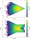 |
Fig. 1 Spatial distribution of the BJ sample after applying the cuts described in Sect. 2. The top panel shows the x–y plane, whereas the bottom panel shows the R–z plane. |
3 Jeans equations in the MW
The Jeans equations stem from taking velocity moments of the collisionless Boltzmann equation assuming steady-state equilibrium. In the case of axisymmetry the natural coordinates are cylindrical (R, ϕ, ɀ). The radial Jeans equation, relating to the gravitational force in the radial direction and thus to the circular velocity curve, is (Eq. (4.222a) in Binney & Tremaine 2008):
 (1)
(1)
where Φ(R, ɀ) is the Galactic potential, v(R, ɀ) is the density distribution of the tracer population and 〈⋅〉 signifies the mean of the given quantity. Equivalent equations can be written down for the vertical and azimuthal components (but the latter is trivially satisfied in the case of axisymmetry as ∂Φ/∂ϕ = 0). Equation (1) reveals that the radial force depends on the second moments of the velocity distributions, their derivatives and the density of the tracers.
To derive the circular velocity curve from this Jeans equation, we rewrite Eq. (1) as
 (2)
(2)
where we have defined that  . The second term in this equation is known as the asymmetric drift term, and the third is the crossterm. We model v with an analytical function of the form:
 (3)
(3)
where we assume Rexp = 3 kpc and hɀ = 0.3 kpc (Ou et al. 2024; Bland-Hawthorn & Gerhard 2016). This represents a disc-like number density, which is appropriate since our sample is dominated by stars in the MW disc. In Sects. 4.2 and 7 we discuss the effects of using these values (and of other assumptions) on our results.
To estimate the velocity moments at a given radius, we bin the stars linearly in R with a width of 0.5 kpc starting at the Galactic centre. We calculate the errors in our bins through bootstrapping. To deconvolve results from the measurement errors, it is necessary to first calculate  , where
  is the variance of the υR distribution in a bin, and σobs is the propagated error to this quantity from the measurement errors. We find that the effect of deconvolution with measurement errors is small since they are typically only ~0.01% of our statistical errors when combined with the bootstrapping error.
Selections performed to make the different samples considered in this work and their number of data points.
3.1 Second moments: 〈vR2〉, 〈vϕ2〉 and 〈vz2〉
Figure 2 shows the radial profiles and distributions of the BJ sample, with scattered red points depicting  calculated for each radial bin. We do not show bins with less than 15 stars since they typically produce spurious values with large errors. The background distribution shows the histogram of ||(υυT − C)ii)|| for each star in the sample. Here, υυT signifies the velocity tensor for that star, and C signifies the covariance matrix of the observational errors for that star.
For R < 6 kpc, the effect of the Galactic bar cannot be neglected, particularly if it is a long bar as some recent works suggest (Wegg et al. 2015; Portail et al. 2017; Sormani et al. 2022). We therefore exclude this region from our analysis as a clear violation of axisymmetry. From looking at the background histogram in Fig. 2 we find that  is dominated by the mean υϕ, whereas the other two velocity moments are dominated by dispersion since the bulk of the stars have a lower value of the velocity tensor than the radial profile of
  . There are clear ridges visible in the background histogram for
  , corresponding to the ridges reported in Antoja et al. (2018), Kawata et al. (2018) and Ramos et al. (2018).
In Fig. 3, we show our inferred radial profiles. The results based on the BJ and SH samples agree within uncertainties for  and
and  . We have also plotted the O23 results in this figure. Beyond R ≳ 17 kpc, our bins typically contain less than ~50 stars and thus suffer from low-number statistics. This is where the differences with O23 are largest. Their smaller distance errors enable them to reach farther out in the disc. The differences for <17 kpc in the azimuthal second moment (which is systematically lower than that from O23), can be almost entirely attributed to the difference in solar position and velocity used for coordinate transformations.
To infer υc using Eq. (2) typically a function is fitted to the profile of  to avoid numerically noisy derivatives. In an isothermal disc in dynamical equilibrium with a constant scale height and mass-to-light ratio, the vertical Jeans equation can be used to show that the second moments of υR as well as υɀ should follow an exponential radial profile if one assumes an exponential surface density profile (van der Kruit & Searle 1981):
 (4)
(4)
Under the stated assumptions,  should hold. While this relation has been confirmed to hold in external galaxies, for example by Martinsson et al. (2013), these authors do report deviations for R > 1.5Rexp. This is perhaps not surprising given that at large distances discs may be flaring and hence breaking down the assumption of a constant scale height. Nonetheless, following previous works, we fit this profile in a radial range between 6 < R < 15 kpc (see the top panel of Fig. 3). The typical exponential scale length we find for the selections listed in Table 1 is
  , which is not too different from the expected 2Rexp.
The radial profile of  deviates from the fitted exponential profile from R ≈ 12.5 kpc onward, as can be seen also in Fig. 2. The deviation from the exponential profile for the second moments of υR and υɀ is less pronounced for the SH sample but is still present. This means that the magnitude of the deviation is only slightly dependent on the specifics of the sample selection, but its existence is independent of the sample used. The flattening of the second moment in υR is also seen in O23 and Zhou et al. (2023), but is attributed to a much larger exponential scale-length (indeed the data are fitted out to ~30 kpc). The work by O23 find
  , similar to that reported by Zhou et al. (2023), who report a value of 24 kpc. While such a fit does not work well for our data (it overpredicts the dispersion at R ~ 10–12 kpc, and underpredicts the trend at large distances, although this can be due to distance errors), it is indicative of an assumption that does not fully hold in the modelling, likely related to the flaring of the MW disc.
To study asymmetric behaviour in the MW disc, we divided our samples in various subsets (see Table 1 for details on these selections). The first division was made by separating the sample above (ɀ > 0, BJz+) and below (ɀ < 0, BJz−) the disc plane. Figure 4 shows the radial profiles of the BJz+ and BJz- samples. The most striking feature is how the profiles of the three velocity components are different for the various subsets. In vR, the moments above and below the plane start deviating from an exponential profile at R > 12.5 kpc, with BJz+ having higher values than BJz−. In υϕ, the split happens at R > 11 kpc with BJz- being above BJz+, in agreement with Gaia Collaboration (2021a), see their Fig. 12. In υɀ, we see oscillating behaviour, where the different subsamples have crossing points at R = 10, 13 and 16 kpc. So while the disc kinematics are symmetric with respect to the Galactic plane within R ≈ 11 kpc, beyond this radius, this is clearly not the case.
We have also inspected the dependence of the second moments on azimuth by splitting the sample in wedges of 15° each. The results are shown in Fig. B.1, and although some differences are apparent, they are of smaller amplitude than the asymmetry with respect to the Galactic disc plane.
Figure 5 shows the distribution of the difference between samples BJz+ and BJz− of the three second moments of the velocity in the x − y-plane. Here, we can see clear antisymmetry both azimuthally and vertically throughout the MW disc. While υR and υɀ show depict differences of up to 10 km s−1 for R < 10 kpc, υϕ shows more asymmetry, up to 20 km s−1.
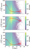 |
Fig. 2 Second moments of the velocity components for the BJ sample. From top to bottom, the panels show |


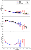 |
Fig. 3 Comparison of the three radial profiles of the second moments in υR, υϕ, and υɀ (from top to bottom) in the MW stellar disc for the BJ (red) and SH (blue) samples. The dotted lines in the top panel are the exponential profile fit from Eq. (4). The error bars show the bootstrapping error from binning. The black dots show the radial profiles from Fig. 3 from O23, and the olive dashed line shows the exponential profile fit to their points. The difference in υϕ between our results and those from O23 is due to a difference in assumed solar velocity parameters and slight differences in the sample. |
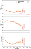 |
Fig. 4 Comparison of the three radial profiles of the second moments of υR, υϕ, and υɀ (from top to bottom) in the MW stellar disc for the BJ sample split into a sample above (ɀ > 0, blue) and below (ɀ < 0, red) the disc plane. |
3.2 The correlation 〈υRυz〉 and crossterm
The crossterm (the final term in Eq. (2)) is typically neglected in calculations of the circular velocity curve (see e.g. Eilers et al. 2019; Ou et al. 2024; Jiao et al. 2023, who estimate the contribution to vc to be smaller than a few percent). To estimate its magnitude for our dataset, we first find the correlation 〈υRυɀ〉(R,ɀ), using additional bins in ɀ with a width of 0.25 kpc. To calculate the value of 〈υRυɀ〉 at greater heights above and below the disc plane we relax the cut in vertical coordinates to |ɀ| < 5 kpc. The error bars are estimated by bootstrapping the sample in each bin.
The behaviour of 〈υRυɀ〉 throughout the MW disc can be quantified by the tilt angle γ of the velocity ellipsoid:
 (5)
(5)
The tilt angle of the stars in the BJ sample, with the relaxed ɀ cut, can be seen in Fig. 6. For every bin, we plot an ellipse representing the velocity ellipsoid, except for bins with less than 25 stars, which are given by a square marker. If the tilt of the velocity ellipsoid follows a spherical alignment, this reduces to γsph = tan−1(R/ɀ). We define the mismatch between γ and γsph to be γ − γsph for ɀ < 0 and γsph − γ for ɀ > 0. This mismatch with respect to spherical alignment is given by the colour coding in Fig. 6. We find that the velocity ellipsoids seem to be more aligned with the plane of the stellar disc than with a spherical coordinate system, in agreement with Hagen et al. (2019). However, there is also some asymmetry in the ɀ = 0 plane for |ɀ| > 1.5 kpc.
For calculating the influence of the crossterm in vc as function of radius, we proceeded to fit a profile to 〈υRυɀ〉 to estimate ∂〈υRυɀ〉/∂ɀ in Eq. (2). We chose to fit a linear profile here, such that we can write the crossterm as
 (6)
(6)
where 〈υRυɀ〉(ɀ) = Az + C. In the fully axisymmetric case, 〈υRυɀ〉 is expected to follow a linear profile that passes through the origin (C = 0). To estimate the slope A, we fit the data for |ɀ| < 1 kpc using eight bins (see Fig. 7). We find that a linear fit to the correlation 〈υRυɀ〉 is still reasonable, although the data does not necessarily cross the origin. Previous work by Silverwood et al. (2018) fitted 〈υRυɀ〉 = Azn for only ɀ > 0, a profile that also assumes that the correlation crosses the origin, and hence cannot capture the asymmetry above and below the plane seen in Fig. 7.
The assumption of a linear behaviour seems to break down for |ɀ| > 0.5 kpc for R = 7.25 kpc, and we see a slight deviation from linear behaviour at 8.25 and 9.25 kpc as well. Even though the linearity seems to hold within |ɀ| < 0.75 kpc for R > 10 kpc again (although for R = 14.25 kpc nonlinear behaviour may be apparent, it had to assess given the low number of stars), this is where a clear offset of 〈υRυɀ〉 from crossing the origin starts. This offset is very likely due to the warp present in the MW disc, whose mean ɀ-coordinate is indeed negative for R > 10 kpc and for the Galactic longitudes probed by our sample (see e.g. Skowron et al. 2019; Cabrera-Gadea et al. 2024 or Jónsson & McMillan 2024 for a first analysis of the effect of the warp on the local dynamics). These findings imply the need to be careful in interpreting results from the axisymmetric Jeans equations at ɀ = 0 as the plane of symmetry no longer coincides with ɀ = 0.
4 The velocity curve of the Milky Way and its uncertainties
4.1 Derivation of the circular velocity curve
By combining the individual terms of Eq. (2), we calculate the circular velocity curve for our samples and present it in Fig. 8.
This figure reveals a decline in our inferred circular velocity curve that starts at R ~ 7.5 kpc and continues at least out to R ∼ 15 kpc. This is in good agreement with the previous studies of Wang et al. (2023), Zhou et al. (2023) Ou et al. (2024) and Jiao et al. (2023) and that are shown as shaded regions, within the statistical uncertainties of these studies for R > 12 kpc. For R < 12 kpc, the difference in our results from those from O23 is mostly caused, as discussed earlier, by a difference is assumed solar velocity. For large distances, R > 17.5 kpc, our derivation of the circular velocity curve starts to suffer from the effects of low number statistics.
Splitting our sample above and below the disc plane reveals a statistically significant difference of ~8km s−1 the circular velocity curve using data located above or below the plane. This difference is a direct consequence of the split observed in the middle panel of Fig. 5, which is driven by the behaviour of  , which is asymmetric with respect to the Milky Way disc plane This is likely due to the Galactic warp. While at R > 18 kpc asymmetries also are apparent, this is also where our uncertainties sharply increase, and we are unable to assess whether the circular velocity curve follows a more steep decline as reported in Wang et al. (2023); Ou et al. (2024); Zhou et al. (2023).
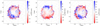 |
Fig. 5 Difference between the distributions of the second moments of υR, υϕ, and υz (from left to right) for the BJz+ and BJz- samples. We use evenly spaced bins in x and y of width 0.5 kpc. The colour bars were limited to within the 1σ value of the distribution of calculated |

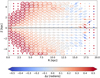 |
Fig. 6 Misalignment of the velocity ellipsoid with respect to spherical alignment in radians, plotted in cylindrical coordinated R, ɀ . For ɀ > 0 this is defined as γ − γsph and for ɀ < 0 as γsph − γ. Square markers denote bins with less than 25 stars. We only plotted every other bin of width 0.25 kpc in R and ɀ for clarity of the figure. |
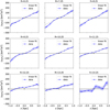 |
Fig. 7 Vertical profile of the correlation 〈υRυɀ〉 for different bins in R. The shaded region shows the bootstrapped error from binning. The dashed grey line is a linear fit to the data between |ɀ| < 1. The dashed black line can guide the eye to where the correlation crosses the origin. The origin is denoted with a black dot. |
4.2 Assessment of the systematic uncertainties
The systematic uncertainties caused by our various assumptions are summarised in Fig. 9, which is similar to figures presented in previous studies such as the earlier cited Eilers et al. (2019), Zhou et al. (2023), Ou et al. (2024) and Jiao et al. (2023). Individually, under R ≈ 18 kpc the systematic effects discussed here are below 5%, which is of order 11.5 km s−1.
Number density profile: The selection function of our survey is arguably too poorly understood to recover an accurate number density of the tracer population, forcing us to assume a given analytic profile. We choose exponential decline (Eq. (3)) with a scale length of Rexp = 3 kpc following previous works. The light green (dark green) solid lines in Fig. 9 show the systematic shift expected for the calculated υc when we lower (raise) Rexp by 1 kpc. This can have an effect up to 5% in the outer regions and to 2% within R < 14 kpc. The size of the effect of raising Rexp is smaller than that of lowering it by the same amount, and thus summarising this uncertainty into one line is a misrepresentation. Alternatively, O23 investigated the systematic differences found by modelling the number density as a power law instead, finding a greater systematic uncertainty beyond 10 kpc. We return to this point in Sect. 7.
Radial velocity profile: To compute a smooth derivative of the radial velocity profile
 we assume and fit an exponential profile (Eq. (4)). However, this does not describe the data well for R > 12.5 kpc (see Fig. 3). If the data are instead fitted in the region of 11 < R < 22 kpc, we obtain a much larger scale-length of 43 kpc, which reflects the flattening off seen at large radii in
  for our dataset. The grey dotted line in Fig. 9 shows the difference found from using the larger scale length on the rotation curve, which amounts to 2.5% for R < 13 kpc, and up to 5% at large radii.
-
Asymmetries and spatial selection: The Jeans equations we apply assume a time-independent, axisymmetric potential. As shown through vertical or azimuthal cuts in Sect. 3.1, this assumption is not true throughout the disc. The red (blue) dash-dotted lines in Fig. 9 show the effect of only looking at the sample below (above) the disc, whilst the purple (orange) dashed lines show the effect of looking only at the wedge in -30 < ϕ < 0° (0 < ϕ < 30 °). Each of these selections has an effect that can be as large as 3%.
Additionally, we find less restrictive spatial selections have approximately a 1–2% effect on our results. Extending the cut in |ɀ| from < 1 kpc to < 5 kpc has only an effect of about 0.5% on the results for υc. Relaxing the additional 6° wedge in ɀ, chosen to ensure the dataset includes the flaring of the disc, impacts results by less than 1%. These results suggest that our results do not depend strongly on the specific choice of spatial selection.
Crossterm: The contribution of the crossterm in Eq. (6) is shown as the brown dotted line, and its contribution is under 0.5% for R ≤ 17 kpc and can be neglected when compared to other systematic effects.
Local Standard of Rest: A difference in the value of the local standard of rest velocity can cause a systematic shift in
 , correspondingly of up to 3% in υc at any given radius (Fig. 8). This estimate is slightly larger than that by O23, who separately tested the effect of changing the Sun’s distance to the Galactic centre and the proper motion of SgrA* within their errors. This shift (visible in Fig. 3) is the likely cause of the differences between our results and those of O23 for R < 12 kpc.
We note that different selections or systematics can shift the resulting vc at each radius either up or down, and combining these effects into a single error estimate is not trivial because they are not independent or Gaussian in nature (see e.g. Oman & Riley 2024, for a discussion of the impact of this assumption). In a worst-case scenario, assuming that they are independent, they could add up in quadrature to give an error of ~6% for R < 14 kpc and up to 15% at larger radii. This is in accordance with the findings from O23, Jiao et al. (2023) and typically larger than estimated by Zhou et al. (2023).
This is particularly relevant in the context of recent attempts to determine the density profile of the Galaxy’s dark matter halo by fitting the circular velocity curve (as done in e.g. Ou et al. 2024; Jiao et al. 2023). These works favour halos with a steep outer slope or cutoff, which is driven by a declining rotation curve for R > 15 kpc. The uncertainties in our dataset prevent us from seeing such a steep decline beyond this radius. In any case, this region is where the systematic uncertainties are higher, and it is important to recall that a 15% systematic uncertainty on the circular velocity results in a 30% uncertainty on the mass enclosed at these radii.
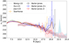 |
Fig. 8 Rotation curves calculated for several samples from Table 1. The black and orange lines show the BJ and SH samples, respectively. The blue and red lines show the BJz+ and BJz− samples, respectively. The grey, light blue, and pink lines and shaded regions show the results from Wang et al. (2023), O23, and Jiao et al. (2023), respectively. |
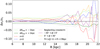 |
Fig. 9 Systematic uncertainties when using Jeans equations to calculate υc. Lines show the difference between different selections or methods and the fiducial BJ model. The light green (dark green) solid line shows the systematic shift when changing the exponential scale length of the number density by −1 kpc (1 kpc). The red (blue) dash-dotted line shows the variation expected considering samples below (above) the disc, selecting ɀ < 0 (ɀ > 0) only. The red dotted line shows the influence of the crossterm in Eq. (6). The dashed purple and orange lines show Δυc/υc for samples for which −30 < ϕ < 0° and 0 < ϕ < 30° respectively. The dotted grey line shows the influence of trying to fit |


5 N-Body simulations of an interaction with a heavy perturber
To investigate the effectiveness of the radial Jeans equation in recovering the circular velocity curve of a system, we apply our Jeans methodology to two simulation suites of MW-like galaxies. This also allows us to study possible causes of the asymmetry we found in data from Gaia DR3 and their likely impact on the derived υc(R) for the MW. In this section we focus on the Simulation L2 from Laporte et al. (2018), an N-body simulation of a MW-like galaxy interacting with a satellite system like the Sagittarius dwarf.
Time stamps of interest in the L2 simulation from Laporte et al. (2018) considered in this work.
5.1 Description of the simulation L2
The Sagittarius progenitor in the L2 simulation has an initial mass of M200 = 6.0 × 10¹⁰M⊙. This relatively large mass leaves a remnant of Sagittarius that is arguably too massive at present day compared to observations. Nonetheless, it successfully reproduces qualitatively important observables like the phase space spiral, and the Monoceros and TriAnd structures in Gaia DR2 (Laporte et al. 2019). The initial conditions of the disc stars were generated to reproduce in broad terms the Milky Way. For example, the density profile described by an exponential disc with a scale length of Rexp = 3.5 kpc, which is also what we use in our application of Jeans equation. For each snapshot, the disc was aligned by iteratively finding the centre of mass, and then aligning the ɀ-axis to the angular momentum of the inner disc (as done in e.g. Laporte et al. 2018; García-Conde et al. 2024). We can thus expect similar complications from a warp present in the disc of L2 as we saw for the MW (see Sect. 3.2).
We select simulation samples using the disc particles in two 60° wedges on opposite sides of the disc, denoted as x < 0 and x > 0. We repeat our spatial selection from Sect. 2, with a cut in |ɀ| < 0.5 kpc instead of 1 kpc. This change affects our results by less than 1%.
We specifically choose six snapshots in this simulation, corresponding to just before or after a pericentre passage of the satellite (see Table 2). These pericentres are the moments when the satellite has the strongest dynamical effects on the disc and demonstrate the impact on the Jeans modelling the clearest. The first two pericentres of the satellite are at ~30 kpc and ~20 kpc respectively, while the other pericentres are within ~15 kpc. The mass of the satellite is still significant at the later 3 passages while interacting more directly with the disc system.
The true velocity curve of the simulation can be calculated as  , with aR being the acceleration in the R-direction due to the gravitational force enacted. We exclude particles belonging to the satellite, which typically have negligible effect outside of the satellites pericentre, and they are not a part of the system we want to apply Jeans equations to. We estimate the intrinsic variation of υc,true around the disc by calculating υc,true in wedges of 15 degrees around the disc and calculating the dispersion at each radius.
5.2 Applying Jeans equations to L2
The radial profiles of the second velocity moments, calculated for the snapshots at times ti from Table 2, can be seen in Fig. 10, which can be compared to Fig. 3. The top row shows results for x < 0 for all snapshots except t6 , which we show in the bottom row with additional cuts in ɀ ≶ 0 and x ≶ 0. Initially (at t1 ) the disc is dynamically relaxed and symmetric and  and
and  follow an exponential decline. At later times, we see an increase in these second moments in the outskirts of the disc. This effect is larger just after an interaction (t2,4,5,6), and then as the disc relaxes the effect decreases (t3), although it never vanishes at large radii.
The second moment for υϕ depicts wiggles which reflect the formation of spiral arms in the disc as can be seen from the light blue curve for t3 . The first interaction indeed produces tidally induced spiral arms as seen in Figs. 14 and 15 from Antoja et al. (2022) using the same simulation. Furthermore, we can see the effect of the longer dynamical timescale in the outer disc region. While the second moment of υR follows the exponential profile for R < 20 kpc for t3, it shows a deviation for R > 20 kpc, similar to the deviation for R > 12.5 kpc just after the first pericentre at t2.
At t4 (after the second pericentre) and t5 , the dispersions of the velocities are high, and we see how the interactions move the disc further toward disequilibrium and asymmetries. For t6 we see clear differences in the recovered second moments for x>0 and x < 0, and also a split in the profiles above and below the plane, even though the overall behaviour is similar. The split is less pronounced for υR and υɀ than it is for υϕ. This split is likely related to bulk motions arising in disc stars in the outer disc due to the interactions with the satellite. We found a similar split in the MW data (see Fig. 4), where there is a difference up to 10 km s−1 at R ≈ 13 kpc. In contrast, in this simulation the magnitude can be as high as 40 km s−1 as seen for x < 0 at R ≈ 22 kpc. This is potentially due to the interactions with a much heavier Sagittarius, as its larger mass could be the driver of the much larger asymmetry seen than measured for the MW.
Figure 11 shows the vc calculated for our six snapshots along with the azimuthally averaged value of υc,true and its 1σ quantiles. The left panel shows the results for all snapshots but t6 , and t6 itself is plotted in the right panel for the same spatial selections as in the bottom row of Fig. 10. The departures from the initial equilibrium configuration (at t1 ) that were seen in Fig. 10 at higher radii are imprinted in the circular velocity curve as well for all other snapshots. These include the wiggles corresponding to the spiral arm structure at t3 , t4, t5 , and t6 and the splits in the profiles for t6 with ɀ ≶ 0. We see that a higher deviation from a dynamically relaxed and symmetric system (i.e. seen in snapshot t1) is also reflected in a larger mismatch with υc,true.
The time evolution of the difference Δυc = υc − υc,true can be seen in Fig. 12 for the samples x > 0 and x < 0 located on opposite sides of the disc throughout the time of the simulation. We now only averaged υc,true over the azimuthal wedge under consideration. Between the first pericentres, the Δυc shows a structure of diagonal stripes that are the result of the tidally induced bi-symmetric spiral arms, alternating between areas of overestimating and underestimating the υc(R). On average, there is a tendency to overestimate υc at R > 15 kpc in both sides of the disc, and to underestimate it at inner radii. We also looked at the side of the disc at a 90-degree angle (y > 0) and found that the sign of Δυc is opposite to the slices at x ≶ 0 but they also show an overall trend of overestimating (underestimating) at the outer (inner) disc regions at later times.
For later pericentres, the density structures are more complex and do not show perfect 2-fold symmetry. Hence, the circular velocity is underestimated for x < 0 (top panel) and overestimated for x > 0 (middle panel). During the third pericentre, the satellite more directly interacts with the disc system while still being very massive, which is reflected in the larger values for Δυc.
The bottom panel shows the intrinsic variation with azimuth of υc,true. The RMS of υc,true at t1 is negligible, while at t6 this intrinsic variation covers a range of ~20 km s−1. The RMS increases slightly between R = 10–15 kpc after each pericentre, and the formation of a bar is apparent after the third pericentre. The dispersion in the outer regions of the disc remains steady for most of the time. We have also found in the snapshots that the disc plane is not consistently at ɀ = 0 after the third pericentre, especially in the outer regions. This further increases the over- and underestimations in υc seen in the top and middle panels of Fig. 12 over the whole range in R as the disc is highly perturbed around these times. The shift of mean ɀ determined for snapshots after the third pericentre can reach values of |(ɀ)| = 1.5 kpc in the outer regions of the disc. Laporte et al. (2018) already showed that the presence of Sgr causes a torque on the disc both through the wake in the halo and its own interactions, which are the likely causes of this misalignment. We conclude from Fig. 12 that the Jeans equations cannot recover  within 5% for R > 8 kpc from the third pericentre onward, and that this mismatch is typically larger (up to 15%) for higher radii, and can be either an over- or underestimation.
In summary, we find similar behaviour in the L2 simulation as that resulting from the analysis of the BJ sample, namely both a flattening off of 〈υR〉 and 〈υz〉 and an asymmetry in  with respect to the disc plane. However, we do not expect the deviations from the true υc,true in the MW to be as big as those in this idealised simulation with a satellite that is likely more massive than the Sagittarius dwarf galaxy (Laporte et al. 2019; Antoja et al. 2018).
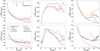 |
Fig. 10 Radial profiles of the three second moments of the velocity distribution in simulation L2 from Laporte et al. (2018). The top row shows t{1,2,3,4,5}. The bottom row shows t6 for both sides of the disc in x ≶ 0 and vertical cuts in ɀ ≶ 0, along with the equilibrium situation at t1 for reference. |
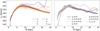 |
Fig. 11 υc calculated for the different snapshots in simulation L2 from Laporte et al. (2018). The dotted lines show the azimuthally averaged value of υc,true, with the shaded region showing the 1σ quantiles of the intrinsic variation. The left panel shows t{1,2,3,4,5}, corresponding to the top row of Fig. 10. The right panel corresponds to the bottom row of Fig. 10, showing the results for t6 in different slices for x ≶ 0 and ɀ ≶ 0. |
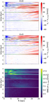 |
Fig. 12 Time-evolution of υc in the simulation from Laporte et al. (2018). Top and middle: the difference between the Jeans equation derived υc and the true υc,true. The top panel shows the result for x < 0 and the middle panel shows the opposite side of the disc (x > 0). Bottom: the RMS of υctrue with azimuth. Green (white) horizontal lines show the pericentres of the satellite. The start of the simulation is at t = 0. |
6 Cosmological simulations
To gain even more insight in the applicability of Jeans equations to infer υc, we also apply our methodology to the six simulated galaxies from the Auriga project (Grand et al. 2017), and their corresponding Gaia mocks known as Aurigaia (Grand et al. 2018). This project is a suite of high-resolution magneto-hydrodynamical zoom-in cosmological simulations of MW-sized galaxies (Grand et al. 2017), originally comprising of 30 simulations labeled Au1 to Au30 at resolution level 4. Six of the original 30 haloes (Au6, Au16, Au21, Au23, Au24, Au27) were then resimulated at a higher resolution (level 3) with a dark matter particle mass of mDM = 4 × 10⁴ M⊙, a stellar particle mass of mb = 6 × 10³ M⊙, and a softening parameter ϵ = 184 pc. The properties of the galaxies can be found in Table 3. Of the 6 halos, Au6 is considered a close analogue of the MW considering its stellar mass, star formation rate, and morphology. Au16 and Au24 have larger discs than the MW, and Au21, Au23, and Au27 have had some combination of heavy, recent, and frequent satellite interactions (Grand et al. 2018). For these analyses, the coordinate system has been chosen such that the Z-axis is the eigenvector of the inertia tensor of the particles within 0.1R200 that is most aligned with the largest angular momentum vector of the same particles in the original simulation frame (Grand et al. 2017).
For these 6 high-resolution simulations, the Auriga project created a mock Gaia DR2-like catalogue (see Grand et al. 2018 for details). First, each star particle was expanded into full stellar populations, drawn from isochrones defined by the star particles’ metallicity and age using a Chabrier Initial Mass Function (IMF, Chabrier 2003). The stars’ positions and velocities are then distributed around the approximate phase space volume of the parent star particle by a 6D smoothing kernel, as described in Lowing et al. (2015). These phase-space positions correspond to the ‘true’ positions and velocities of the stars, which can then be transformed to ‘observed’ Galactic coordinates when choosing a fixed position for the Sun. From the absolute values of the stars magnitude and colours, the apparent values are calculated, and an additional effect of dust extinction is applied. Only stars with G < 20 are included in the Aurigaia mock samples, simulating the Gaia DR2 observability limit. The original Aurigaia catalogues were created using approximates for the expected Gaia DR2 errors using the apparent magnitudes, colours, and distances of the stars. For this work, we recalculate the mock observational errors to resemble Gaia DR3-like errors using the PYGAIA1 software package. The observed DR3 mock values of the star are then the true values convolved with these errors.
We therefore have three different stellar datasets for every Auriga halo; the original simulation star particles, the true stars without any observational errors, and the DR3 mock stars. Accompanying this, the Auriga project supplies force grids of the final snapshots of the six galaxies, which we can use to find υc,true in the simulation as we did in Sect. 5 by azimuthally averaging over the force grid. The force found in this way is consistent with the force found by directly averaging the gravitational force stored for all simulation particles for the provided snapshot in the same spatial selection as described in Sect. 2.
For all samples, we perform a similar spatial cut to our MW sample described in Sect. 2. The cut in |ɀ| < ɀcut and the angle α of the wedge in ɀ is adapted to incorporate the thickness and flare (if present) of the disc of the simulated galaxy. This flare is characterised by Rflare, which is found by fitting hz(R) ∝ exp(R/Rflare) (Grand et al. 2017). The cut |ɀ| < zcut is taken to be three times the scale height at solar radius, 3hz,8kpc, so that α = tan−1(zcut/Rflare), which reflects the spatial cut made for the data but scaled to the disc of the simulations. We also remove stars with |υɀ| > 100 km s−1.
To simulate a Gaia DR3 RVS selection, we select stars with G < 14. For the mock stars, we demand additional quality cuts following our MW selection in Sect. 3; requiring a relative error in parallax smaller than 20%, and making the same red giant stars selections in Teff and log(ɡ). Distances are estimated by inverting the parallax, and the transformation from ‘observed’ to Galactic coordinates is made with the ‘true’ solar parameters used to generate the mock. Furthermore, we require the simulation particles that the mock stars were generated from also follow our spatial cuts.
Disk parameters for the MW and Auriga galaxies.
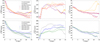 |
Fig. 13 Radial profiles of the second moments of the velocity for the six Aurigaia mocks from Grand et al. (2018). The top row has results for Au6, Au16, and Au21, the bottom row shows Au23, Au24, and Au27. Scattered points with error bars show the results for the mock samples described in Table 3 while solid lines show the result for the stellar particles in the final simulation snapshot of the simulated galaxies. The dashed lines in the left column show the exponential fit to the profile of the mock sample, while the dotted lines show the fit to the profile of the simulation particle sample. |
6.1 Applying Jeans equations to Auriga
Figure 13 shows the radial profiles of the velocity moments for the observed mock samples (symbols with error bars) and the stellar particles (solid lines with shaded regions) in the final snapshot of the simulation for the six Auriga galaxies. We see that  for the mock sample does not follow an exponential decline from R ≈ 10 kpc onward, rather showing a similar behaviour to the Gaia DR3 data and the simulation of the interaction of a Sagittarius-like satellite from Sect. 5. Following our approach to the MW, we fit the exponential profile to
  in the radial range where the profile is a good description of the data.
The second moment in υϕ of the mock sample shows considerable features indicating deviations from equilibrium and axisymmetry in all galaxies, for instance the wiggles indicating spiral arms in Au21 (orange curve). For  we see similar deviations from an exponential decline as for
  , but due to the lower dispersions the variations are less pronounced here. For the sample of mock stars, we typically see a less pronounced departure from an exponential decline for both υR and υɀ compared to the simulation particles, as well as less distinct features in υϕ pointing to disequilibrium. Especially for the higher radii this is partially due to the contamination from halo star particles, since there is no specific selection of the simulation particles, apart from the requirement that |υz| < 100 km s−1.
We have also studied the vertical asymmetry in the Auriga systems by again splitting up the sample in a cut above and below the disc. We find a similar behaviour in the profiles to that seen in the data in Fig. 4. The difference between the samples above and below the disc is of a similar magnitude to the data as well, and smaller than seen in the simulation in Sect. 5 (Fig. 10). Au6 is most similar in the magnitude of this asymmetry when compared to the MW.
Figure 14 shows different estimations of the circular velocity curve for all six galaxies. The black line and corresponding grey-shaded region show υc,true and its intrinsic variation with azimuth throughout the disc, following our approach in Sect. 5. We typically see a spread of ~1.5% around the azimuthally averaged profile. The green dashed line shows υc calculated from applying the Jeans equations to the simulation particles in the final snapshot, using the radial profiles shown with solid lines in Fig. 13.
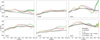 |
Fig. 14 Jeans derived υc for the six Aurigaia mocks from Grand et al. (2018). The green dashed line with shaded region shows the result for the simulation particles. The orange line shows the result for the full mock catalogue with only a magnitude limit at G < 20. The red points show the results for the full mock with our data quality cuts. The blue points show the result for the observed mock sample. This is the sample shown in Fig. 13 and described in Table 3. The black line and shaded region show υc,true and its associated 1σ variation. |
6.2 The effects of sample selection
We now consider the differences between the results obtained for the simulation particles, true stars, and mock observed stars. To estimate the effect of the RVS selection function on our results we consider the full stellar catalogue; similar to the true star catalogue but relaxing the RVS magnitude limit of G < 14 to the G < 20 magnitude limit of the Aurigaia catalogues. Additionally, we require the parent simulation particles of the star also satisfy our spatial selection. The orange line in Fig. 14 shows the result for this full stellar catalogue. Compared to the green line it shows the additional effect of having a selection function applied to the tracer population sample. We also study the effect of our quality cuts. By applying these to the full mock sample we end up with the red points in Fig. 14. Lastly we can see the effect of the measurement errors by looking at the observed mock sample. This is shown as the blue points in Fig. 14, and corresponds to the symbols with error bars in Fig. 13.
From these results we see that the simulation particles (green dashed lines) typically provide the closest match to ≳c,true (black line in Fig. 14), with approximately a 5% over- or underestimation on average. We also see that the simulation particle results tend to start overestimating υc,true for R ≳ 20 kpc, which is due to the fact that the disc ends around that radius, so our sample is starting to be dominated by stellar halo particles. The wiggles in the simulation particle result for Au21 and Au23 at R < 15 kpc are due to spiral arm structure in the disc (Gómez et al. 2017).
We typically see a 5–10% mismatch between υc and υc,true for the full mock catalogue (orange lines in Fig. 14), which is slightly larger than the result for the simulation particles themselves. We investigate how much of this effect is due to the procedure of generating the mock stars from the simulation particles in Appendix C. We conclude that this effect is typically of the order of 2–3 km s−1 in υϕ and υR, which is for the most part self-corrected through the asymmetric drift term in Eq. (2). Instead, we attribute this difference between the simulation and the mocks is due to the selection function and limitations of the tracer population.
When we apply our quality cuts, we see that the red points in Fig. 14 tend to be a closer match to the green line (the simulation particles) for R ≲ 15 kpc. The cut in magnitude has the largest impact on the results for υc due to its impact on the selection function of the tracer population. The next most impactful cut is that of selecting only giants. For higher radii the complicated selection function and limited amount of data points increases the mismatch with υc,true and the simulation particles. We also see that observational uncertainties introduce only a small effect after all quality cuts have already been applied (blue points in Fig. 14). For all simulated galaxies except Au16 and Au24 we also see that υc for the mock samples tends to start declining more steeply than υc,true around R ≳ 18 kpc because of selection effects on the sample, even though these discs are embedded in extended dark matter halos that follow relatively well NFW profiles (Callingham et al. 2020).
6.3 Satellite perturbations
Many of the features that we see in the velocity moments and in υc(R) are qualitatively similar to those seen in the simulation L2 discussed in Sect. 5. They can again be attributed to the perturbations of satellites by considering the recent accretion history of the Auriga galaxies. Since these galaxies have had a more complex, cosmological history than the idealised L2 simulation, they can show more complex structure, due to, for instance, the recoiling and precessing of the disc or the asymmetric torques on the disc system caused by the unique merger history:
Au6 suffers a large accretion event 8 Gyr ago at a mass ratio with the host of 1 : 12. This satellite only fully disrupted 0.5 Gyr ago, after orbiting the host halo with apocentres at ~40 kpc and pericentres at ~20 kpc. This is likely to have dynamically heated the stellar disc, as can be seen in the profiles for the second moments of the velocity in Fig. 13. It’s disc is atypical and does not follow the expected behaviour: an exponential decline in υR and υɀ and an approximately constant profile for υϕ after R > 12 kpc. A significant part of this behaviour is sufficiently corrected for when calculating υc with Eq. (2), as seen in Fig. 14.
Au16 has had a quiescent merger history over the past 4 Gyr, and has not suffered significant recent perturbations to the dynamical equilibrium of the disc system. As a result, its derived υc is close to υc,true.
Au21 has the largest difference between υc and υc,true. The galaxy accreted a satellite 5.5 Gyr ago with a mass ratio to the host of 1 : 15, that survives to present day, with a recent pericentre at 15 kpc only 0.5 Gyr ago. This has caused significant perturbations to the disc, as evident in its velocity profiles.
Au23 has had a satellite which fully disrupted in the host only 2.2 Gyr ago, but has had a quiet merger history since. The existence of the wiggles in the second moments and υc within R < 15 kpc is likely due to disequilibrium structure.
Au24 had three satellites that fully disrupted ~2 Gyr ago, but has had a quiet merger history since then. Hence we expect some disequilibrium in the disc system, and due to the longer dynamical timescale of the outer disc, we can also explain the larger mismatch with υc,true in this way.
Au27 has suffered 7 satellites of various infall times and mass ratios, and various distances from the disc system. It is less clear which of these has likely had the largest effect on the disc dynamics and the results in Fig. 14, but Au27 is clearly being impacted by its satellite dynamics.
These results reaffirm our conclusion from Sect. 5 that a satellite or system of satellites interacting with a disc system, combined with observational limits and a complicated selection function can cause a mismatch in the inferred υc and υc,true of 5–15%, as well as a declining trend for large radii in a Jeans derived rotation curve.
7 Discussion
As can be concluded from the results presented in Sect. 4 on the analysis of the Gaia data and the simulations in Sects. 5 and 6, several intricacies underlie the practice of calculating the circular velocity curve through the application of Jeans equations under the assumption of equilibrium and axisymmetry. In this section we re-emphasise the caveats and complications that arise and which need further scrutiny.
7.1 Sample selection and distances
Comparing our results to previous studies, we see slight differences in the behaviour of the radial profiles of the second moments of the various velocity components. These differences are due to a combination of the specific survey used for the data, the sample selection, distance estimation, and the assumed solar parameters.
One selection we do not apply is a cut in [α/Fe] < 0.12 to remove contamination from the thick (high-alpha) disc, as performed in O23 using the APOGEE data of their sample. We used the catalogue of calibrated metallicities from Recio-Blanco et al. (2023) to study the effect of the cut in [α/Fe] < 0.12, but restricting our sample this way limited our data to R < 14 kpc, and our results did not change within this radius.
In our study of the MW, we see a change in the behaviour of the radial profiles of all second velocity moments around R ≈ 12.5–15 kpc, in agreement with previous work (Ou et al. 2024; Zhou et al. 2023; Jiao et al. 2023; Wang et al. 2023). This distance corresponds to a heliocentric distance of ~4–7 kpc, beyond which distance estimates typically have a larger dispersion when compared to stars that are closer to the Sun (Hogg et al. 2019; Anders et al. 2022; Bailer-Jones 2023). While as we discuss below this is unlikely to be the reason behind the plateau in  , our analysis of the simulations in Fig. 14 shows that a distance quality cut can in fact produce an artificial decline in υc at high radii even when υc,true does not show evidence thereof. We refer the reader to Luri et al. (2018) for a more general discussion of distance quality and sample selection effects.
7.2 Systematics on the rotation curve
As described and shown in Fig. 9, the individual specific changes in the spatial selection or parameters of the model only affect the results systematically up to 2% within R < 12.5 kpc and 5% up to R < 20 kpc. In the worst case, combining several of these systematics together can lead up to a 6% effect for the inner radii and 15% for the outer radii. In the simulations however, both N-body and cosmological, we see that υc(R) derived through Jeans equations can differ from υc,true(R) up to 5–15% as well. Hence the methodological approach of applying the time-independent, axisymmetric Jeans equations to a system showing signs of dynamical disequilibrium is certainly a source of mismatch.
For example, we find evidence of a departure from an exponential profile for  in the MW, in the sense of a flattening off for R > 12.5 kpc. This is also present in the data of Zhou et al. (2023) and O23, but was instead interpreted as implying a larger scale-length, which is however not expected in steady-state configurations for systems with a constant scale height (and we note that the MW’s disc is known to be flared). In Sect. 6, we see that the plateau is more apparent for simulation particles than for the mock, although we do observe a departure from the exponential profile around R ~ 12 kpc in most simulated galaxies. From the simulations, we see that any bulk motion, satellite interaction, (transient) spiral structure, or other dynamical structure can impact this feature. We conclude that the plateau is most likely due to a history of satellite interactions that caused non-equilibrium and asymmetric dynamical signatures.
Another systematic effect relates to the representation of the density of the tracer population. We have assumed an exponential density profile, but it has been suggested that the thin disc could be truncated around a radius of R = 15 kpc (see e.g. Minniti et al. 2011, but see also López-Corredoira et al. 2018). Although we do not have evidence of a sharp truncation, we do see a sharp decrease in the numbers of stars at large radii (see the histogram in Fig. 2). Additionally, the flare and the warp in the MW disc become important around R ≳ 12.5 kpc, and we saw the effect of the latter in Fig. 7. An important follow-up step is to include the effect of the warp on the modelling, like in Cabrera-Gadea et al. (2024) or Jónsson & McMillan (2024). Furthermore, the assumed axis of symmetry of ɀ = 0 is not necessarily in the right position (Chrobáková et al. 2022; Bovy et al. 2016), and we see evidence of this also in the velocities’ second moments. Therefore, an important improvement could be made in the treatment of the spatial density of our tracer population, which enters υc(R) through how we calculate the asymmetric drift correction term. We come back to this point below.
7.3 A Keplerian decline of the Galactic rotation curve?
A surprising result of recent work on the Galactic circular velocity curve is the claim of a Keplerian decline by Jiao et al. (2023). Although not of similar amplitude, we do find a declining trend starting from R ≳ 18 kpc for the υc(R) inferred using the Jeans equation for all halos except Au16, even though these discs are embedded in a dark matter halo. Trying to fit a dark matter halo to such profiles would require a more pronounced outer slope or cutoff, and would likely result in a low virial mass.
Yet, the biggest source of uncertainty and possibly bias at larger distances lies in the density profile of the tracer population, particularly if this is affected by some kind of truncation. If we neglect the cross-term in Eq. (2), the difference in the circular velocity that could arise when assuming a density profile vn compared to that obtained with the originally assumed v is
 (7)
(7)
In the top panels of Fig. 15 we compare the density profiles of the exponential disc v from Eq. (3) to two models of smoothly truncated discs  for n = 2,4, with Rmax = 20 kpc. Since we can rewrite
  , then
 (8)
(8)
where we have assumed that Δυc/υc is small. The bottom panel of Fig. 15 shows Δυc, assuming that  km/s at R > 15 kpc and a linear decline for υc(R) = υc,⊙ − β(R − R⊙) as in Jiao et al. (2023), where υc,⊙ is the circular velocity at R⊙, the solar position, and β = −2.18 km s−1 kpc−1.
Figure 15 thus reveals that the circular velocity inferred from the Jeans equation assuming a pure exponential profile could be underestimated by up to ~10 km s−1 at 30 kpc for n = 2, and ~45 km s−1 for n = 4, which is large enough to account for the steep decline seen for the MW (see Jiao et al. 2023; Wang et al. 2023). We perform a slightly more in-depth study of this effect in Appendix D and find again that modelling a truncated disc with an exponential density profile leads to an underestimated υc in the outskirts. Therefore, this effect could potentially explain the declining rotation curve presented in other works and would leave room for a flat rotation curve for the Milky Way (as the decline is fully compensated by not accounting properly for the density profile of the population). It is thus of great importance to determine reliably the density profile of the outer Galactic disc.
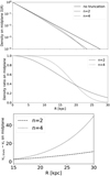 |
Fig. 15 Top: Comparison of the density profiles from an exponential disc to two slowly truncated disc models. Bottom: Difference in the inferred circular velocity for the above models compared to an exponential disc. |
8 Summary and conclusions
The main goal of this study is to investigate the validity of applying the radial Jeans equation under the assumptions of steady-state and axisymmetry to the MW in order to derive its circular velocity curve, in particular given the recently reported signatures of disequilibrium in our Galaxy (Widrow et al. 2012; Williams et al. 2013; Gaia Collaboration 2021a; Antoja et al. 2018; Vasiliev et al. 2021; Gaia Collaboration et al. 2023a). To this end, we studied the behaviour of the different terms in the axisymmetric Jeans equations in the MW stellar disc up to a galactocentric radius of R ~ 21 kpc using data from Gaia DR3 (Gaia Collaboration et al. 2023b). We measured the second moments of the velocity  throughout the MW disc. Using these terms, we proceeded to derive the circular velocity curve υc for the MW, obtaining similar results to recent literature. We verified our methodology using two numerical simulations: the N-body simulation L2 of a MW galaxy interacting with a Sagittarius dwarf (Laporte et al. 2018) and the Auriga cosmological simulations (Grand et al. 2017). Our analyses lead us to the following conclusions:
The kinematics of disc stars in the MW show vertical asymmetries, and also change with azimuth, providing further evidence that the MW is not in dynamical equilibrium (Figs. B.1, 2, 5, and 4 and Sect. 3). However, we find that using the methodology of this paper to calculate the circular velocity curve υc of the MW using Jeans equations is robust within ~5% for R < 14 kpc when considering only systematics intrinsic to the methodology (Figs. 8 and 9 and Sect. 4.2). Additionally, including the crossterm in Eq. (2) has no significant impact on these calculations of the MW rotation curve (Sect. 3.2);
The radial profiles for
 and
and  do not follow the expected exponential declining behaviour for a disc in equilibrium (i.e. with
  ). The departure from an exponential declining behaviour is also seen in simulated MW-like systems that have had interactions with satellites that led to dynamical perturbations, such as spiral arms, flares, or bulk motions across the stellar disc (Figs. 3, 10, and 14 and Sects. 4, 5, and 6);
Such interactions are the most likely effect that can cause the observed non-equilibrium signatures in the circular velocity curve derived through the radial Jeans equation (Figs. 14, 10, 12, and 13 and Sects. 5 and 6). The mismatch with υc,true is further impacted when considering observational limitations or a complicated selection function in the tracer population. From the simulations, we infer that these effects combined can cause a systematic uncertainty of up to 15% (Figs. 12 and 14). For the galaxy in the Auriga suite that most resembles the MW (Au6), we find a systematic uncertainty of smaller than 10% (which translates to an error of 20% in the enclosed mass).
Furthermore, if the density of the tracer population were truncated at large radii but were not taken into account in the Jeans modelling, this could result in a significant mismatch (e.g. of order 45 km s−1), which could be incorrectly interpreted as a fast declining rotation curve (7.3).
We have thus uncovered similar problems in modelling the mass content of our Galaxy using the Jeans equations to Kafle et al. (2018), El-Badry et al. (2017), Wang et al. (2018), and Kretschmer et al. (2021), only that we are studying the axisymmetric case as opposed to the spherical case (see also Chrobáková et al. 2020). Nonetheless, to first order, we find that the radial Jeans equation is a useful tool for deriving the circular velocity curve for the MW. However, with data of the quality available in the modern era, we now see the impact of higher-order effects and systematic uncertainties resulting from simplifications and broken assumptions. We therefore urge that caution be exercised when interpreting vc values calculated through Jeans equations with the current methodology outside of R > 15 kpc, as this region is particularly affected by asymmetries, the warp and flare of the MW disc, and kinematic disturbances (Sect. 7).
The systematic uncertainties associated with the data sample could be reduced by increasing the quantity and quality of measurements of the kinematics of disc stars at large distances. The most significant improvements will likely come from more flexible modelling methodologies. It is also important to investigate the possibility of abandoning the assumptions of time-independence and axisymmetry when deriving a Galactic rotation curve, as this could potentially lead to higher precision.
Acknowledgements
We thank the referee for their constructive report, and we thank Robert Grand who kindly provided clarifications regarding the Auriga simulations used in this work. OK also thanks Christine Eilers and Xiaowei Ou for sharing their data and insights with us, as well as Friedrich Anders and Eugene Vasiliev for helpful discussions. We are grateful to Filippo Fraternali for scientific interactions and literature suggestions. We acknowledge financial support from a Spinoza prize to AH. The work reported on in this publication has been partially supported by COST Action CA18104: MW-Gaia. TA acknowledges the grant RYC2018-025968-I funded by MCIN/AEI/10.13039/501100011033 and by ‘ESF Investing in your future”, the grants PID2021-125451NA-I00 and CNS2022-135232 funded by MICIU/AEI/10.13039/501100011033 and by ‘ERDF A way of making Europe”, by the ‘European Union’ and by the ‘European Union Next Generation EU/PRTR’ and the Institute of Cosmos Sciences University of Barcelona (ICCUB, Unidad de Excelencia ‘María de Maeztu’) through grant CEX2019-000918-M. This work has made use of data from the European Space Agency (ESA) mission Gaia (https://www.cosmos.esa.int/gaia), processed by the Gaia Data Processing and Analysis Consortium (DPAC, https://www.cosmos.esa.int/web/gaia/dpac/consortium). Funding for the DPAC has been provided by national institutions, in particular the institutions participating in the Gaia Multilateral Agreement. Throughout this work, we have made use of the following packages: astropy (Astropy Collaboration 2013), vaex (Breddels & Veljanoski 2018), SciPy (Virtanen et al. 2020), matplotlib (Hunter 2007), NumPy (van der Walt et al. 2011), GADGET-4 (Springel et al. 2021), AGAMA (Vasiliev 2019) and Jupyter Notebooks (Kluyver et al. 2016).
Appendix A Figures for the StarHorse sample
For readability of the main manuscript we present the distributions for the SH sample here, since they agree qualitatively with the results on the BJ sample.
Appendix B Azimuthal split for the Bailer-Jones sample
Figure B.1 shows the radial profiles for the BJ sample split up into azimuthal slices of 15°. We can see how there appears to be a trend in  and
and  in that they decrease overall with increasing ϕ, seen by the light blue points generally lying above the darker blue, purple and pink points in the leftmost and rightmost panels of Fig. B.1.
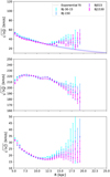 |
Fig. B.1 Comparison of the three radial profiles of the second moments of the velocity distributions in the Milky Way stellar disc for the BJ sample split into four smaller azimuthal slices between (−30°, −15°, 0°, 15°, 30°). |
Furthermore, the azimuthal second moment seems to be slightly lower for the wedges further away from the anticentre, and higher for those at lower azimuths, which is likely to be a selection effect due to poor sampling. We included two lines in Fig. 9 showing the effect of taking 30° wedges to avoid selection effects, and can conclude that there is asymmetry in azimuth in the Milky Way disc.
Appendix C Aurigaia mock particles
As described in Grand et al. (2018) and Lowing et al. (2015), to generate the Gaia DR2 mock catalogues for the six Aurgaia halos, a population of stars is generated for each particle in the final simulation snapshot. As seen in Fig. 14, the mock sample for a given Auriga halo will typically have a larger Δυc than the sample with simulation particles. In this appendix we investigate what is the driving force behind this larger Δυc. We present results for studying this effect only in halo Au6, but similar findings hold for the other halos.
For each mock star, the particle ID of the simulation particle that it was spawned from is stored in the mock catalogue. We call this simulation particle the ‘parent particle’. Thus we can find the sample of parent particles that have generated the mock particles in our selected sample. Typically, except for the region of ≈ 1.5 kpc around the solar position, the parent samples contain fewer particles than the simulation particle sample discussed in Sect. 6. Near the Sun, υc for parent particles is equal to the υc found for the simulation particles. Also, in any region further away from the Sun, some of the simulation particles in the parent sample are not within our spatial selection, but end up in the sample because they have generated a mock particle that did end up in our selection. These parent particles inflate the tails of the velocity distribution of particles in the relevant radial bins, thereby inflating the dispersion and thus the second moments of the velocity distributions as well. That is why we opt to minimise this numerical effect by keeping only mock stars that were generated from parent stars within our spatial selection.
C.1 Effect of generating a mock sample
A final question can be asked about the generating of mock particles from the simulation particles and if it causes some artificial dispersion to our mock sample. To investigate this artificial dispersion, we start by finding all parent particles of stars in our mock sample. Then, for each parent particle, we look at all mock stars spawned from that particle that are present in our mock. We calculate the dispersion of this group of stars, and their mean velocity. This mean velocity often differs from the velocity of the parent particle, creating a nonzero Δυ. Figure C.1 shows the radially binned and averaged profiles of these dispersions and displacements.
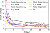 |
Fig. C.1 Radial profiles of the average dispersion and displacement of the mock particles with respect to their parent particles. Black lines show the total over all three velocity components. Solid (dashed) lines show the dispersion (displacement). Red, blue and green lines show the values for υR, υϕ and υz respectively. |
We see here that we can expect an artificial mean displacement of particles in velocity of about 3 km/s, and a dispersion of about 4 km s−1. This is contrary to the quite good match within 2% between the mock and simulation results (the blue points and green dashed line, respectively) in Fig. 14. When calculating υc, the artificial dispersion and displacement in υϕ get mostly self-corrected through the asymmetric drift term (the second term in Eq. 2), which is why this does not influence our result for υc more than 1 – 2%. The additional dispersion from generating the mock particles does explain part of the mismatch between the radial profiles for the same samples in Fig. 13. Still, we find that the sample selections and selection function are more important in causing the differences seen in Fig. 14.
Appendix D Action distribution models of truncated discs
To test the effects of a truncated disc, we consider a set of toy models, generated by action distributions in a fixed potential using AGAMA (Vasiliev 2019). We model the thin disc using the QuasiIsothermal DF, which gives a number density profile and radial velocity dispersion profile that are very close to exponential. We use the following parameters: Rdisk = 3 kpc, Hdisk = 0.2 kpc, σr,0 = 75 km s−1, and Rσ,r = 25 kpc. We note that Rσ,r corresponds to the exponential scale length of  , and is equivalent to twice that of
  .
.
To model truncated discs, we modified the QuasiIsothermal DF to
 (D.1)
(D.1)
where Rmax is the truncation radius, and n gives the steepness of the truncation. We use Rmax = 20 and n = 4.
From these distributions, we draw positions and velocities of 10 million tracer particles, that follow physical selections of 6 kpc < R < 25 kpc and |ɀ| < 0.1 kpc. These particles are purely a tracer population and has no effect on the underlying galactic potential, which is fixed to the potential of McMillan (2017). Upon these particles, we perform the same modelling as we apply to the MW. We fit exponential profiles to the radial velocity, finding that they approximately follow the parameters of the distribution function. The crossterm is approximated using a dataset with a relaxed physical selection of |ɀ| < 1 kpc.
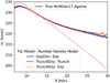 |
Fig. D.1 The results of applying Jeans Modelling to find the velocity curves from samples drawn from action distributions. We create samples of tracer particles drawn from three different models, a model representing an approximately exponential disc, and two models where the disc has been truncated, with the Trunc4 model sharply truncated. The solid lines correspond to velocity curves found using number densities that correctly match the action distribution model. The dotted lines show the results of incorrectly assuming that the truncated samples follow an exponential number density. |
For the number density profile, we model the truncated discs with both the true corresponding truncated number density profile, and a best-fit exponential profile. The results can be seen in Fig. D.1. When the true number density of the tracer population is known, the velocity curve is well recovered (solid curves), and closely matches the true value of the potential. The small differences between the true velocity curve and the correct models can be attributed to the small difference between the true number density generated by the action distribution models and the analytic exponential and truncated exponential profiles.
However, if the tracer population is truly distributed as a truncated profile and is instead modelled as exponential, strong systematic effects appear. The recovered velocity curve has a noticeable decline, with a slope of β ≈ −1.5km s−1 kpc−1. A sharper truncation, with larger n, or a smaller Rmax, constitute a stronger decline.
References
- Ablimit, I., & Zhao, G. 2017, ApJ, 846, 10 [Google Scholar]
- Anders, F., Khalatyan, A., Queiroz, A. B. A., et al. 2022, A&A, 658, A91 [NASA ADS] [CrossRef] [EDP Sciences] [Google Scholar]
- Andrae, R., Rix, H.-W., & Chandra, V. 2023, ApJS, 267, 8 [NASA ADS] [CrossRef] [Google Scholar]
- Antoja, T., Helmi, A., Romero-Gómez, M., et al. 2018, Natur, 561, 360 [NASA ADS] [CrossRef] [Google Scholar]
- Antoja, T., Ramos, P., López-Guitart, F., et al. 2022, A&A, 668, A61 [NASA ADS] [CrossRef] [EDP Sciences] [Google Scholar]
- Antoja, T., Ramos, P., García-Conde, B., et al. 2023, A&A, 673, A115 [NASA ADS] [CrossRef] [EDP Sciences] [Google Scholar]
- Astropy Collaboration (Robitaille, T. P., et al.) 2013, A&A, 558, A33 [NASA ADS] [CrossRef] [EDP Sciences] [Google Scholar]
- Bañares-Hernández, A., Castillo, A., Martin Camalich, J., & Iorio, G. 2023, A&A, 676, A63 [NASA ADS] [CrossRef] [EDP Sciences] [Google Scholar]
- Bailer-Jones, C. A. L. 2023, AJ, 166, 269 [NASA ADS] [CrossRef] [Google Scholar]
- Bailer-Jones, C. A. L., Rybizki, J., Fouesneau, M., Demleitner, M., & Andrae, R. 2021, AJ, 161, 147 [Google Scholar]
- Binney, J., & Tremaine, S. 2008, Galactic Dynamics: Second Edition [Google Scholar]
- Bland-Hawthorn, J., & Gerhard, O. 2016, ARA&A, 54, 529 [Google Scholar]
- Bosma, A. 1981, AJ, 86, 1825 [NASA ADS] [CrossRef] [Google Scholar]
- Bovy, J., Prieto, C. A., Beers, T. C., et al. 2012, ApJ, 759, 131 [NASA ADS] [CrossRef] [Google Scholar]
- Bovy, J., Rix, H.-W., Schlafly, E. F., et al. 2016, ApJ, 823, 30 [NASA ADS] [CrossRef] [Google Scholar]
- Breddels, M. A., & Veljanoski, J. 2018, A&A, 618, A13 [NASA ADS] [CrossRef] [EDP Sciences] [Google Scholar]
- Cabrera-Gadea, M., Mateu, C., Ramos, P., et al. 2024, MNRAS, 528, 4409 [NASA ADS] [CrossRef] [Google Scholar]
- Callingham, T. M., Cautun, M., Deason, A. J., et al. 2019, MNRAS, 484, 5453 [Google Scholar]
- Callingham, T. M., Cautun, M., Deason, A. J., et al. 2020, MNRAS, 495, 12 [NASA ADS] [CrossRef] [Google Scholar]
- Cautun, M., Benítez-Llambay, A., Deason, A. J., et al. 2020, MNRAS, 494, 4291 [Google Scholar]
- Chabrier, G. 2003, PASP, 115, 763 [Google Scholar]
- Chrobáková, Ž., López-Corredoira, M., Sylos Labini, F., Wang, H. F., & Nagy, R. 2020, A&A, 642, A95 [NASA ADS] [CrossRef] [EDP Sciences] [Google Scholar]
- Chrobáková, Ž., Nagy, R., & López-Corredoira, M. 2022, A&A, 664, A58 [NASA ADS] [CrossRef] [EDP Sciences] [Google Scholar]
- de Blok, W. J. G., Walter, F., Brinks, E., et al. 2008, AJ, 136, 2648 [NASA ADS] [CrossRef] [Google Scholar]
- Eilers, A.-C., Hogg, D. W., Rix, H.-W., & Ness, M. K. 2019, ApJ, 871, 120 [Google Scholar]
- El-Badry, K., Wetzel, A. R., Geha, M., et al. 2017, ApJ, 835, 193 [NASA ADS] [CrossRef] [Google Scholar]
- Gaia Collaboration (Antoja, et al.) 2021a, A&A, 649, A8 [NASA ADS] [CrossRef] [EDP Sciences] [Google Scholar]
- Gaia Collaboration (Brown, A. G. A., et al.) 2021b, A&A, 649, A1 [NASA ADS] [CrossRef] [EDP Sciences] [Google Scholar]
- Gaia Collaboration (Drimmel, et al.) 2023a, A&A, 674, A37 [CrossRef] [EDP Sciences] [Google Scholar]
- Gaia Collaboration 2023b, A&A, 674, A1 [NASA ADS] [CrossRef] [EDP Sciences] [Google Scholar]
- García-Conde, B., Antoja, T., Roca-Fàbrega, S., et al. 2024, A&A, 683, A47 [NASA ADS] [CrossRef] [EDP Sciences] [Google Scholar]
- Genzel, R., Förster Schreiber, N. M., Übler, H., et al. 2017, Natur, 543, 397 [NASA ADS] [CrossRef] [Google Scholar]
- Gómez, F. A., Grand, R. J. J., Monachesi, A., et al. 2017, MNRAS, 472, 3722 [CrossRef] [Google Scholar]
- Grand, R. J. J., Gómez, F. A., Marinacci, F., et al. 2017, MNRAS, 467, 179 [NASA ADS] [Google Scholar]
- Grand, R. J. J., Helly, J., Fattahi, A., et al. 2018, MNRAS, 481, 1726 [Google Scholar]
- Gravity Collaboration 2018, A&A, 615, L15 [NASA ADS] [CrossRef] [EDP Sciences] [Google Scholar]
- Hagen, J. H. J., Helmi, A., de Zeeuw, P. T., & Posti, L. 2019, A&A, 629, A70 [NASA ADS] [CrossRef] [EDP Sciences] [Google Scholar]
- Haines, T., D’Onghia, E., Famaey, B., Laporte, C., & Hernquist, L. 2019, ApJ, 879, L15 [Google Scholar]
- Hogg, D. W., Eilers, A.-C., & Rix, H.-W. 2019, AJ, 158, 147 [Google Scholar]
- Hunter, J. D. 2007, Comput. Sci. Eng., 9, 90 [NASA ADS] [CrossRef] [Google Scholar]
- Jiao, Y., Hammer, F., Wang, H., et al. 2023, A&A, 678, A208 [NASA ADS] [CrossRef] [EDP Sciences] [Google Scholar]
- Jónsson, V. H., & McMillan, P. J. 2024, A&A, 688, A38 [NASA ADS] [CrossRef] [EDP Sciences] [Google Scholar]
- Jurić, M., Ivezic, Ž., Brooks, A., et al. 2008, ApJ, 673, 864 [NASA ADS] [CrossRef] [Google Scholar]
- Kafle, P. R., Sharma, S., Robotham, A. S. G., Elahi, P. J., & Driver, S. P. 2018, MNRAS, 475, 4434 [NASA ADS] [CrossRef] [Google Scholar]
- Kamada, A., Kaplinghat, M., Pace, A. B., & Yu, H.-B. 2017, PhRvL, 119, 111102 [NASA ADS] [Google Scholar]
- Kawata, D., Baba, J., Ciuca, I., et al. 2018, MNRAS, 479, L108 [Google Scholar]
- Kluyver, T., Ragan-Kelley, B., Pérez, F., et al. 2016, in Positioning and Power in Academic Publishing: Players, Agents and Agendas, eds. F. Loizides, & B. Scmidt (IOS Press), 87 [Google Scholar]
- Kretschmer, M., Dekel, A., Freundlich, J., et al. 2021, MNRAS, 503, 5238 [NASA ADS] [CrossRef] [Google Scholar]
- Laporte, C. F. P., Johnston, K. V., Gómez, F. A., Garavito-Camargo, N., & Besla, G. 2018, MNRAS, 481, 286 [Google Scholar]
- Laporte, C. F. P., Minchev, I., Johnston, K. V., & Gómez, F. A. 2019, MNRAS, 485, 3134 [Google Scholar]
- Lelli, F., McGaugh, S. S., & Schombert, J. M. 2016, AJ, 152, 157 [Google Scholar]
- López-Corredoira, M., Allende Prieto, C., Garzón, F., et al. 2018, A&A, 612, L8 [EDP Sciences] [Google Scholar]
- Lowing, B., Wang, W., Cooper, A., et al. 2015, MNRAS, 446, 2274 [NASA ADS] [CrossRef] [Google Scholar]
- Lucy, L. B. 1974, AJ, 79, 745 [Google Scholar]
- Luri, X., Brown, A. G. A., Sarro, L. M., et al. 2018, A&A, 616, A9 [NASA ADS] [CrossRef] [EDP Sciences] [Google Scholar]
- Majewski, S. R., Schiavon, R. P., Frinchaboy, P. M., et al. 2017, AJ, 154, 94 [NASA ADS] [CrossRef] [Google Scholar]
- Mancera Piña, P. E., Fraternali, F., Oosterloo, T., et al. 2022, MNRAS, 514, 3329 [CrossRef] [Google Scholar]
- Martinsson, T. P. K., Verheijen, M. A. W., Westfall, K. B., et al. 2013, A&A, 557, A130 [NASA ADS] [CrossRef] [EDP Sciences] [Google Scholar]
- McMillan, P. J. 2017, MNRAS, 465, 76 [NASA ADS] [CrossRef] [Google Scholar]
- Minniti, D., Saito, R. K., Alonso-García, J., Lucas, P. W., & Hempel, M. 2011, ApJ, 733, L43 [Google Scholar]
- Mróz, P., Udalski, A., Skowron, D. M., et al. 2019, ApJ, 870, L10 [Google Scholar]
- Navarro, J. F., Frenk, C. S., & White, S. D. M. 1996, ApJ, 462, 563 [Google Scholar]
- Oman, K. A., & Riley, A. H. 2024, MNRAS, 532, L48 [NASA ADS] [CrossRef] [Google Scholar]
- Oman, K. A., Navarro, J. F., Fattahi, A., et al. 2015, MNRAS, 452, 3650 [CrossRef] [Google Scholar]
- Ou, X., Eilers, A.-C., Necib, L., & Frebel, A. 2024, MNRAS, 528, 693 [NASA ADS] [CrossRef] [Google Scholar]
- Petersen, J., & Lelli, F. 2020, A&A, 636, A56 [NASA ADS] [CrossRef] [EDP Sciences] [Google Scholar]
- Pont, F., Queloz, D., Bratschi, P., & Mayor, M. 1997, A&A, 318, 416 [NASA ADS] [Google Scholar]
- Portail, M., Gerhard, O., Wegg, C., & Ness, M. 2017, MNRAS, 465, 1621 [NASA ADS] [CrossRef] [Google Scholar]
- Ramos, P., Antoja, T., & Figueras, F. 2018, A&A, 619, A72 [NASA ADS] [CrossRef] [EDP Sciences] [Google Scholar]
- Read, J. I., Iorio, G., Agertz, O., & Fraternali, F. 2016, MNRAS, 462, 3628 [NASA ADS] [CrossRef] [Google Scholar]
- Recio-Blanco, A., de Laverny, P., Palicio, P. A., et al. 2023, A&A, 674, A29 [NASA ADS] [CrossRef] [EDP Sciences] [Google Scholar]
- Reid, M. J., & Brunthaler, A. 2004, ApJ, 616, 872 [Google Scholar]
- Roman-Oliveira, F., Fraternali, F., & Rizzo, F. 2023, MNRAS, 521, 1045 [NASA ADS] [CrossRef] [Google Scholar]
- Rubin, V. C., Burstein, D., & Thonnard, N. 1980, ApJ, 242, L149 [NASA ADS] [CrossRef] [Google Scholar]
- Sands, I. S., Hopkins, P. F., Shen, X., et al. 2024, arXiv e-prints [arXiv:2404.16247] [Google Scholar]
- Schönrich, R., Binney, J., & Dehnen, W. 2010, MNRAS, 403, 1829 [NASA ADS] [CrossRef] [Google Scholar]
- Silverwood, H., Sivertsson, S., Read, J., Bertone, G., & Steger, P. 2018, in Astrometry and Astrophysics in the Gaia Sky, 330, eds. A. Recio-Blanco, P. de Laverny, A. G. A. Brown, & T. Prusti, 255 [NASA ADS] [Google Scholar]
- Skowron, D. M., Skowron, J., Mróz, P., et al. 2019, Science, 365, 478 [Google Scholar]
- Sofue, Y. 2020, Galax, 8, 37 [NASA ADS] [CrossRef] [Google Scholar]
- Sofue, Y., Honma, M., & Omodaka, T. 2009, PASJ, 61, 227 [NASA ADS] [Google Scholar]
- Sormani, M. C., Gerhard, O., Portail, M., Vasiliev, E., & Clarke, J. 2022, MNRAS, 514, L1 [NASA ADS] [CrossRef] [Google Scholar]
- Springel, V., Pakmor, R., Zier, O., & Reinecke, M. 2021, MNRAS, 506, 2871 [NASA ADS] [CrossRef] [Google Scholar]
- van der Kruit, P. C. & Searle, L. 1981, A&A, 95, 105 [NASA ADS] [Google Scholar]
- van der Walt, S., Colbert, S. C., & Varoquaux, G. 2011, Comput. Sci. Eng., 13, 22 [Google Scholar]
- Vasiliev, E. 2019, MNRAS, 482, 1525 [Google Scholar]
- Vasiliev, E., Belokurov, V., & Erkal, D. 2021, MNRAS, 501, 2279 [NASA ADS] [CrossRef] [Google Scholar]
- Virtanen, P., Gommers, R., Oliphant, T. E., et al. 2020, Nature Methods, 17, 261 [CrossRef] [Google Scholar]
- Wang, W., Han, J., Cole, S., et al. 2018, MNRAS, 476, 5669 [NASA ADS] [CrossRef] [Google Scholar]
- Wang, W., Han, J., Cautun, M., Li, Z., & Ishigaki, M. N. 2020, Sci. China Phys. Mech. Astron., 63, 109801 [NASA ADS] [CrossRef] [Google Scholar]
- Wang, H.-F., Chrobáková, Ž., López-Corredoira, M., & Sylos Labini, F. 2023, ApJ, 942, 12 [NASA ADS] [CrossRef] [Google Scholar]
- Wegg, C., Gerhard, O., & Portail, M. 2015, MNRAS, 450, 4050 [NASA ADS] [CrossRef] [Google Scholar]
- Widrow, L. M., Gardner, S., Yanny, B., Dodelson, S., & Chen, H.-Y. 2012, ApJ, 750, L41 [Google Scholar]
- Williams, M. E. K., Steinmetz, M., Binney, J., et al. 2013, MNRAS, 436, 101 [Google Scholar]
- Xue, X.-X., Rix, H.-W., & Zhao, G. 2009, Res. Astron. Astrophys., 9, 1230 [CrossRef] [Google Scholar]
- Zhou, Y., Li, X., Huang, Y., & Zhang, H. 2023, ApJ, 946, 73 [CrossRef] [Google Scholar]
- Zwicky, F. 1933, Helv. Phys. Acta, 6, 110 [NASA ADS] [Google Scholar]
All Tables
Selections performed to make the different samples considered in this work and their number of data points.
Time stamps of interest in the L2 simulation from Laporte et al. (2018) considered in this work.
All Figures
|
Fig. 1 Spatial distribution of the BJ sample after applying the cuts described in Sect. 2. The top panel shows the x–y plane, whereas the bottom panel shows the R–z plane. |
| In the text | |
|
Fig. 2 Second moments of the velocity components for the BJ sample. From top to bottom, the panels show |
| In the text | |
|
Fig. 3 Comparison of the three radial profiles of the second moments in υR, υϕ, and υɀ (from top to bottom) in the MW stellar disc for the BJ (red) and SH (blue) samples. The dotted lines in the top panel are the exponential profile fit from Eq. (4). The error bars show the bootstrapping error from binning. The black dots show the radial profiles from Fig. 3 from O23, and the olive dashed line shows the exponential profile fit to their points. The difference in υϕ between our results and those from O23 is due to a difference in assumed solar velocity parameters and slight differences in the sample. |
| In the text | |
|
Fig. 4 Comparison of the three radial profiles of the second moments of υR, υϕ, and υɀ (from top to bottom) in the MW stellar disc for the BJ sample split into a sample above (ɀ > 0, blue) and below (ɀ < 0, red) the disc plane. |
| In the text | |
|
Fig. 5 Difference between the distributions of the second moments of υR, υϕ, and υz (from left to right) for the BJz+ and BJz- samples. We use evenly spaced bins in x and y of width 0.5 kpc. The colour bars were limited to within the 1σ value of the distribution of calculated |
| In the text | |
|
Fig. 6 Misalignment of the velocity ellipsoid with respect to spherical alignment in radians, plotted in cylindrical coordinated R, ɀ . For ɀ > 0 this is defined as γ − γsph and for ɀ < 0 as γsph − γ. Square markers denote bins with less than 25 stars. We only plotted every other bin of width 0.25 kpc in R and ɀ for clarity of the figure. |
| In the text | |
|
Fig. 7 Vertical profile of the correlation 〈υRυɀ〉 for different bins in R. The shaded region shows the bootstrapped error from binning. The dashed grey line is a linear fit to the data between |ɀ| < 1. The dashed black line can guide the eye to where the correlation crosses the origin. The origin is denoted with a black dot. |
| In the text | |
|
Fig. 8 Rotation curves calculated for several samples from Table 1. The black and orange lines show the BJ and SH samples, respectively. The blue and red lines show the BJz+ and BJz− samples, respectively. The grey, light blue, and pink lines and shaded regions show the results from Wang et al. (2023), O23, and Jiao et al. (2023), respectively. |
| In the text | |
|
Fig. 9 Systematic uncertainties when using Jeans equations to calculate υc. Lines show the difference between different selections or methods and the fiducial BJ model. The light green (dark green) solid line shows the systematic shift when changing the exponential scale length of the number density by −1 kpc (1 kpc). The red (blue) dash-dotted line shows the variation expected considering samples below (above) the disc, selecting ɀ < 0 (ɀ > 0) only. The red dotted line shows the influence of the crossterm in Eq. (6). The dashed purple and orange lines show Δυc/υc for samples for which −30 < ϕ < 0° and 0 < ϕ < 30° respectively. The dotted grey line shows the influence of trying to fit |
| In the text | |
|
Fig. 10 Radial profiles of the three second moments of the velocity distribution in simulation L2 from Laporte et al. (2018). The top row shows t{1,2,3,4,5}. The bottom row shows t6 for both sides of the disc in x ≶ 0 and vertical cuts in ɀ ≶ 0, along with the equilibrium situation at t1 for reference. |
| In the text | |
|
Fig. 11 υc calculated for the different snapshots in simulation L2 from Laporte et al. (2018). The dotted lines show the azimuthally averaged value of υc,true, with the shaded region showing the 1σ quantiles of the intrinsic variation. The left panel shows t{1,2,3,4,5}, corresponding to the top row of Fig. 10. The right panel corresponds to the bottom row of Fig. 10, showing the results for t6 in different slices for x ≶ 0 and ɀ ≶ 0. |
| In the text | |
|
Fig. 12 Time-evolution of υc in the simulation from Laporte et al. (2018). Top and middle: the difference between the Jeans equation derived υc and the true υc,true. The top panel shows the result for x < 0 and the middle panel shows the opposite side of the disc (x > 0). Bottom: the RMS of υctrue with azimuth. Green (white) horizontal lines show the pericentres of the satellite. The start of the simulation is at t = 0. |
| In the text | |
|
Fig. 13 Radial profiles of the second moments of the velocity for the six Aurigaia mocks from Grand et al. (2018). The top row has results for Au6, Au16, and Au21, the bottom row shows Au23, Au24, and Au27. Scattered points with error bars show the results for the mock samples described in Table 3 while solid lines show the result for the stellar particles in the final simulation snapshot of the simulated galaxies. The dashed lines in the left column show the exponential fit to the profile of the mock sample, while the dotted lines show the fit to the profile of the simulation particle sample. |
| In the text | |
|
Fig. 14 Jeans derived υc for the six Aurigaia mocks from Grand et al. (2018). The green dashed line with shaded region shows the result for the simulation particles. The orange line shows the result for the full mock catalogue with only a magnitude limit at G < 20. The red points show the results for the full mock with our data quality cuts. The blue points show the result for the observed mock sample. This is the sample shown in Fig. 13 and described in Table 3. The black line and shaded region show υc,true and its associated 1σ variation. |
| In the text | |
|
Fig. 15 Top: Comparison of the density profiles from an exponential disc to two slowly truncated disc models. Bottom: Difference in the inferred circular velocity for the above models compared to an exponential disc. |
| In the text | |
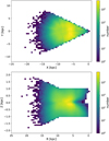 |
Fig. A.1 Same as Fig. 1 but for the SH sample. |
| In the text | |
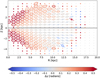 |
Fig. A.2 Same as Fig. 6 but for the SH sample. |
| In the text | |
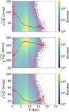 |
Fig. A.3 Same as Fig. 2 but for the SH sample. |
| In the text | |
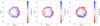 |
Fig. A.4 Same as Fig. 5 but for the SH sample. |
| In the text | |
|
Fig. B.1 Comparison of the three radial profiles of the second moments of the velocity distributions in the Milky Way stellar disc for the BJ sample split into four smaller azimuthal slices between (−30°, −15°, 0°, 15°, 30°). |
| In the text | |
|
Fig. C.1 Radial profiles of the average dispersion and displacement of the mock particles with respect to their parent particles. Black lines show the total over all three velocity components. Solid (dashed) lines show the dispersion (displacement). Red, blue and green lines show the values for υR, υϕ and υz respectively. |
| In the text | |
|
Fig. D.1 The results of applying Jeans Modelling to find the velocity curves from samples drawn from action distributions. We create samples of tracer particles drawn from three different models, a model representing an approximately exponential disc, and two models where the disc has been truncated, with the Trunc4 model sharply truncated. The solid lines correspond to velocity curves found using number densities that correctly match the action distribution model. The dotted lines show the results of incorrectly assuming that the truncated samples follow an exponential number density. |
| In the text | |
Current usage metrics show cumulative count of Article Views (full-text article views including HTML views, PDF and ePub downloads, according to the available data) and Abstracts Views on Vision4Press platform.
Data correspond to usage on the plateform after 2015. The current usage metrics is available 48-96 hours after online publication and is updated daily on week days.
Initial download of the metrics may take a while.