| Issue |
A&A
Volume 648, April 2021
|
|
|---|---|---|
| Article Number | A114 | |
| Number of page(s) | 32 | |
| Section | Interstellar and circumstellar matter | |
| DOI | https://doi.org/10.1051/0004-6361/202039897 | |
| Published online | 23 April 2021 | |
Transition from coherent cores to surrounding cloud in L1688
1
Max-Planck-Institut für extraterrestrische Physik,
Giessenbachstrasse 1,
85748
Garching,
Germany
e-mail: This email address is being protected from spambots. You need JavaScript enabled to view it.
2
Department of Astronomy, The University of Texas at Austin,
Austin,
TX
78712, USA
3
Department of Physics, 4-181 CCIS, University of Alberta,
Edmonton,
AB T6G 2E1, Canada
4
Department of Astronomy & Astrophysics, University of Toronto,
50 St. George St.,
Toronto,
ON M5S 3H4, Canada
5
Observatorio Astronómico Nacional (OAN-IGN),
Alfonso XII 3,
28014,
Madrid, Spain
6
Steward Observatory,
933 North Cherry Ave.,
Tucson,
AZ
85721, USA
7
Ural Federal University,
620002 Mira st. 19,
Yekaterinburg, Russia
8
Department of Physics and Astronomy, University of Victoria,
3800 Finnerty Rd.,
Victoria,
BC V8P 5C2, Canada
9
Herzberg Astronomy and Astrophysics, National Research Council of Canada,
5071 West Saanich Rd.,
Victoria, BC V9E 2E7, Canada
Received:
12
November
2020
Accepted:
9
February
2021
Abstract
Context. Stars form in cold dense cores showing subsonic velocity dispersions. The parental molecular clouds display higher temperatures and supersonic velocity dispersions. The transition from core to cloud has been observed in velocity dispersion, but temperature and abundance variations are unknown.
Aims. We aim to measure the temperature and velocity dispersion across cores and ambient cloud in a single tracer to study the transition between the two regions.
Methods. We use NH3 (1,1) and (2,2) maps in L1688 from the Green Bank Ammonia Survey, smoothed to 1′, and determine the physical properties by fitting the spectra. We identify the coherent cores and study the changes in temperature and velocity dispersion from the cores to the surrounding cloud.
Results. We obtain a kinetic temperature map extending beyond dense cores and tracing the cloud, improving from previous maps tracing mostly the cores. The cloud is 4–6 K warmer than the cores, and shows a larger velocity dispersion (Δσv = 0.15–0.25 km s−1). Comparing to Herschel-based dust temperatures, we find that cores show kinetic temperatures that are ≈1.8 K lower than the dust temperature, while the gas temperature is higher than the dust temperature in the cloud. We find an average p-NH3 fractional abundance (with respect to H2) of (4.2 ± 0.2) × 10−9 towards the coherent cores, and (1.4 ± 0.1) × 10−9 outside the core boundaries. Using stacked spectra, we detect two components, one narrow and one broad, towards cores and their neighbourhoods. We find the turbulence in the narrow component to be correlated with the size of the structure (Pearson-r = 0.54). With these unresolved regional measurements, we obtain a turbulence–size relation of σv,NT ∝ r0.5, which is similar to previous findings using multiple tracers.
Conclusions. We discover that the subsonic component extends up to 0.15 pc beyond the typical coherent boundaries, unveiling larger extents of the coherent cores and showing gradual transition to coherence over ~0.2 pc.
Key words: ISM: kinematics and dynamics / ISM: molecules / ISM: individual objects: L1688 / stars: formation
© S. Choudhury et al. 2021
 Open Access article, published by EDP Sciences, under the terms of the Creative Commons Attribution License (https://creativecommons.org/licenses/by/4.0), which permits unrestricted use, distribution, and reproduction in any medium, provided the original work is properly cited.
Open Access funding provided by Max Planck Society.
1 Introduction
Star formation takes place in dense cores in molecular clouds. Detailed studies of dense cores unveil their physical and chemical properties, which provide the initial conditions in the process of star formation. Across different molecular clouds, the star-forming cores are characterised by higher density and lower temperatures compared to the ambient cloud. Many of the cores also exhibit subsonic turbulence. However, the transition from core to cloud is still not well-understood.
The hyperfine structure of NH3 inversion transitions allows its individual components to remain optically thin at high column densities (Caselli et al. 2017). Unlike carbon-bearing species, such as CO and HCO+, NH3 shows no depletion at high densities and cold temperatures characteristic of cores (Bergin & Langer 1997). Therefore, NH3 is an important and useful high-density tracer of cold gas. Using NH3 (1,1) line emission, Barranco & Goodman (1998) found that the line width inside the four cores studied was roughly constant, and slightly greater than the pure thermal value. These latter authors also reported that at the edge of the cores, the line widths begin to increase. By analysing the cores and their environments, Goodman et al. (1998) suggested that a transition to coherence might mark the boundaries of the dense cores. Using NH3 (1,1) observationswith the Green Bank Telescope, Pineda et al. (2010) studied the transition from inside a core to the surrounding gas, for the first time in the same tracer, and reported a similar, but sharper transition to coherence (an increase in the dispersion by a factor of two in a scale less than 0.04 pc) in the B5 region in Perseus. However, the exact nature of the transition from the subsonic cores to the surrounding molecular cloud is not well known. It is important to study these transition regions, as this could give us clues on how dense cores form and accrete material from the surrounding cloud.
In the Green Bank Ammonia Survey (GAS, Friesen et al. 2017), star-forming regions in the Gould Belt were observed using NH3 hyperfine transitions. Their first data release included four regions in nearby molecular clouds: B18 in Taurus, NGC1333 in Perseus, L1688 in Ophiuchus, and Orion A North. Using the results from this survey and H2 column densities derived with Herschel, Chen et al. (2019) identified 18 coherent structures (termed ‘droplet’) inL1688 and B18. These latter authors observed that these droplets show gas at high density (⟨nH ⟩≈ 5 × 104 cm−3; from massesand effective radii of the droplets, assuming a spherical geometry) and near-constant, almost-thermal velocity dispersion, with a sharp transition in dispersion around the boundary.
The results from Pineda et al. (2010) and Chen et al. (2019) suggest that we can define the boundaries of coherent cores systematically as the regions with subsonic nonthermal line widths. It is to be noted that this approach does not necessarily define cores in the same way as when using continuum emission. Therefore, not all of the ‘coherent cores’ will have continuum counterparts.
The temperature profile inside cores has been studied, and the cores are found to be usually at a temperature ≈10 K (e.g., Tafalla et al. 2002), and more dynamically evolved cores show a temperature drop towards the centre (Crapsi et al. 2007; Pagani et al. 2007). Crapsi et al. (2007) observed a temperature drop down to ≈ 6 K towards the centre of L1544 (see also Young et al. 2004). Pagani et al. (2007) and Launhardt et al. (2013) also reported gradients in temperature outwards from the centres of cores with observations of N2 H+ − N2D+, and far-infrared (FIR)-submillimetre continuum, respectively. However, the transition in gas temperature from cores to their immediate surroundings has not been studied. This is important, as dust and gas are not thermally coupled at volume densities below 105 cm−3 (Goldsmith 2001), as expected in inter-core material (average density in L1688 is ~ 4 × 103 cm−3, see Sect. 2.1). Therefore, the gas temperature can provide important constraints on the cosmic-ray ionisation rate (with cosmic rays being the main heating agents of dark clouds), as discussed in Ivlev et al. (2019). This transition in temperature, as well as in other physical properties, such as velocity dispersion, density and NH3 abundance, from core to cloud, is the focus of the present paper.
In our previous paper (Choudhury et al. 2020, hereafter Paper I) we reported a faint supersonic component along with the narrow core component, towards all cores. We suggested that the broad component traces the cloud surrounding the cores, and therefore, presents an opportunity to study the gas in the neighbourhood of the cores with the same density tracer. Here, we extend that analysis to study the changes in physical properties of these two components from cores to their surroundings.
In this project, we use the data from GAS in L1688 –smoothed to a larger beam – to study the transition in both velocity dispersion and temperature, from coherent cores, to the extended molecular cloud, using the same lines (NH3 (1,1) and (2,2)). In Sect. 2, the primary NH3 data from GAS and complimentary Herschel continuum maps, are briefly described. Section 3 explains the procedure used to determine the physical parameters in the cloud. The improved integrated intensity maps and the parameter maps are presented in Sect. 4. In Sect. 5, the selection of coherent cores, considered in this paper is explained, followed by a discussion on the observed transition of physical parameters and spectra, from cores to their surroundings.
2 Data
2.1 Ammonia maps
As our primary data set, we use the NH3 (1,1) and (2,2) maps, taken from the first data release of Green Bank Ammonia Survey (GAS, Friesen et al. 2017). The observations were carried out using the Green Bank Telescope (GBT) to map NH3 in the star forming regions in the Gould Belt with AV > 7 mag, using the seven-beam K-Band Focal Plane Array (KFPA) at the GBT Observations were made in frequency switching mode with a frequency throw of 4.11 MHz (≈52 km s−1 at 23.7 GHz). The spectral resolution of the data is 5.7 kHz, which corresponds to ≈ 72.1 m s−1 at 23.7 GHz (approximate frequency of observations). The extents of the maps were selected using continuum data from Herschel or JCMT, or extinction maps derived from 2MASS (Two Micron All Sky Survey). To convert the spectra from frequency to velocity space, central frequencies for NH3 (1,1) and (2,2) lines were considered as 23.6944955 and 23.7226333 GHz, respectively (Lovas et al. 2009).
Out of the four regions in the GAS DR1, we focus on L1688 in this paper, as we were able to obtain an extended kinetic temperature map of the cloud for this region. L1688 is part of the Ophiuchus molecular cloud at a distance of ~ 138.4 ± 2.6 pc (Ortiz-León et al. 2018). The cloud mapped in NH3 is ~1 pc in radius with a mass of ≈980 M⊙ (Ladjelate et al. 2020). Assuming spherical geometry and a mean molecular weight of 2.37 amu (Kauffmann et al. 2008), the average gas density is then ~ 4 × 103 cm−3.
The parameter maps of L1688, released in DR1, are not very extended, particularly for kinetic temperature, as a robust temperature measurement is restricted by the signal-to-noise ratio (S/N) of the (2,2) line. Therefore, in order to have a good detection, especially of the (2,2) line, in the outer and less dense part of the cloud, the data were smoothed by convolving them to a beam of 1′ (GBT native beam at 23 GHz is ≈31′′). The data cube was then re-gridded to avoid oversampling. The relative pixel size was kept the same as the original GAS maps, at one-third of the beam-width. The mean root-mean-square (rms) noise level achieved as a result is 0.041 and 0.042 K in the (1,1) and (2,2), respectively. For comparison, the mean noise level in the GAS DR1 maps was 0.17 K. Figure 1 shows the integrated intensity maps obtained for NH3 (1,1) and (2,2).
2.2 H2 column density and dust temperature maps
L1688 was observed in dust continuum using the Herschel space observatory as part of the Herschel Gould Belt Survey (HGBS, André et al. 2010). In order to compare the dust-derived properties to our results with NH3, we use the dust temperature and H2 column density in Ophiuchus from the HGBS archive1 (Ladjelate et al. 2016). These maps were also convolved to a 1′ beam, and then regridded to the same grid as the NH3 maps. Figures 2 and 3 show the smoothed and re-gridded N(H2) and dust temperature maps, respectively.
3 Analysis
3.1 Line fitting
We fit NH3 line profiles to the data with the pyspeckit package (Ginsburg & Mirocha 2011), which uses a forward modelling approach. We follow the fitting process described in Friesen et al. (2017). The range in velocity to fit is determined from the average spectra of the entire region. As the ortho-to-para ratio in the region is not known, we only report the p-NH3 column density here,and do not attempt to convert it to total NH3 column density2.
The model produces synthetic spectra based on the guesses provided for the input parameters : excitation temperature (Tex), kinetic temperature (TK), para-ammonia column density (N(p-NH3)), velocity dispersion (σv) and line-of-sight central velocity (vLSR) of the gas (see Sect. 3.1 in Friesen et al. 2017). A nonlinear gradient descent algorithm, MPFIT (Markwardt 2009) is then used to determine the best-fit model, and corresponding values of the parameters. A good set of initial conditions is necessary toensure that the nonlinear least-squares fitting does not get stuck in a local minimum. The value of vLSR is critical; therefore, we use the first-order moments of the (1,1) line as initial guesses. The second-order moments are used as guesses for velocity dispersion. For the other parameters, we use: 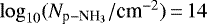 , TK = 20 K and Tex = 5 K. These numbers are within the range of values reported in GAS DR1 maps, and are therefore reasonable guesses. As a test, we checked the fits with varying guesses, and determined that the exact values of the initial parameters does not affect the final results, as long as they are within a reasonable range.
In this work, we use the cold_ammonia model in pyspeckit library, which makes the assumption that only the (1,1), (2,2), and (2,1) levels are occupied in p-NH3. It is also assumed that the radiative excitation temperature, Tex, is the same for (1,1) and (2,2) lines, as well as their hyperfine components.
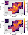 |
Fig. 1 Integrated intensity maps of NH3 (1,1) (top) and (2,2) (bottom) lines. For NH3 (1,1), the contour levels indicate 15σ,30σ, and 45σ, and for NH3 (2,2), contours are shown for 6σ,12σ, and 18σ; where σ is the median error in emitted intensity calculated from the signal-free spectral range in each pixel and converted to the error in integrated intensity. The moment maps were improved by considering only the spectral range containing emission, as described in Sect. 4.1. The 1′ beam, which the data was convolved to, is shown in green in the bottom-left corner, and the scale bar is shown in the bottom-right corner. |
3.2 Data masking
To ensure that the parameters are well determined from the fit, several flags are applied on each parameter, separately. For a good fit to the (1,1) and (2,2) lines, a clear detection is necessary. For centroid velocity, velocity dispersion and excitation temperature, we mask the pixels with a S∕N < 5 in the integrated intensity of the (1,1) line. Similarly, we remove pixels with a S∕N < 3 in the peak intensity of the central hyperfine of the (2,2), in the kinetic temperature and p-NH3 column density maps. These lower limits for the S/N in the (1,1) and (2,2) lines were chosen after a visual inspection of the spectra and the model fits in randomly sampled pixels in order to determine which flags most effectively filtered out the unreliable fits. As we use the pixels with a S/N of 5 or more in the integrated intensity of the (1,1), we expect the excitation temperature, centroid velocity, and velocity dispersion to be determined with reasonably high certainty. Similarly, for kinetic temperature, we only use the pixels with detection of the (2,2) with S/N of 3 in the peak intensity, and therefore TK should also be well determined. Therefore, we mask the pixels with a fit determined error >20% of the corresponding parameter from the TK, vLSR and σv maps. Calculation of N(p-NH3) requires a good determination of excitation temperature, and pyspeckit reports log(N(p-NH3)), and the error in log(N(p-NH3)). We still expect N(p-NH3) to be determined with reasonable accuracy, and therefore we set the relative error cut in N(p-NH3) at 33% (3σ).
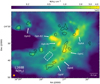 |
Fig. 2 N(H2) in L1688, taken from Herschel Gould Belt Survey archive. Positions of the continuum cores reported in Motte et al. (1998) are indicated by arrows. The dashed rectangle shows the area used to calculate mean cloud properties (see Sect. 4.3). The solid black contours show the coherent cores in the region (described later in Sect. 4.4). The 1′ beam, which the data was convolved to, is shown in orange in the bottom-left corner, and the scale bar is shown in the bottom-right corner. |
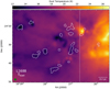 |
Fig. 3 Dust temperature in L1688, taken from Herschel Gould Belt Survey archive. The solid white contours show the coherent cores in the region (described later in Sect. 4.4). The vertical dotted line roughly separates the dark cloud (to the left of the line) from the molecular material affected by the external illumination, due to irradiation from HD147889 (Habart et al. 2003). The 1′ beam, which the data was convolved to, is shown in green in the bottom-left corner, and the scale bar is shown in the bottom-right corner. |
4 Results
4.1 Integrated intensity maps
While calculating the integrated intensity of the region, it is better to use a narrow range of velocities around the velocity at each pixel than using a broad, average velocity range for the entire cloud, because there is a gradient in velocity present among different parts in L1688. Therefore, we employ the procedure described in Sect. 3.2 of Friesen et al. (2017) in deriving the moment maps. We use the best-fit model at each pixel and select the spectral range for which the model shows an intensity > 0.0125 K3. In places where the fit was not satisfactory (based on fit-determined errors), we use the average value of vLSR and σv for the cloud. We then use the known relative positions of the hyperfine transitions of (1,1) and (2,2) to define a range where any emission is expected. We then calculate the integrated emission (and the associated error) using only these channels.
The integrated intensity maps thus obtained for the smoothed data are presented in Fig. 1.
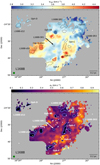 |
Fig. 4 Centroid velocity (top panel) and velocity dispersion (bottom panel) in L1688. The solid black contours in the top panel and solid blue contours in the bottom panel show the coherent cores in the region (described later in Sect. 4.4). The black (top panel) and white (bottom panel) stars show the positions of Class 0/I and flat-spectrum protostars (Dunham et al. 2015). The beam is shown in green in the bottom-left corner, and the scale bar is shown in the bottom-right corner. |
4.2 Property maps
Figures 4–6 show the velocity, velocity dispersion, NH3 kinetic temperature and p-NH3 column density maps for L1688 obtained from our fits. We obtain much more extended maps for velocity dispersion and kinetic temperature(73.4 and 65% of the total observed area, respectively), compared to the original GAS DR1 maps (Figs. 13 and 17 in Friesen et al. 2017, 19.2 and 13% of the total observed area respectively). Also, for the first time, we areable to map the temperature in the dense cores, as well as the surrounding gas in the same density tracer.
In the less dense, outer region of the cloud, the NH3 (1,1) line becomes optically thin, and so, the excitation temperature is harder to determine satisfactorily4. Correspondingly, the p-NH3 column density (Fig. 6) is also not well determined away from some of the continuum cores (identified in Motte et al. 1998).
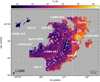 |
Fig. 5 Kinetic temperature in L1688. The solid blue contours show the coherent cores in the region (described later in Sect. 4.4). The white stars show the positions of Class 0/I and flat-spectrum protostars. To see the difference between the part of the cloud affected by the external radiation, and the dark cloud further away from the illuminationsource, we consider a vertical boundary, as shown. The beam is shown in green in the bottom-left corner, and the scale bar is shown in the bottom-right corner. |
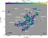 |
Fig. 6 p-NH3 column density in L1688. The solid white contours show the coherent cores in the region (described later in Sect. 4.4). The black stars show the positions of Class 0/I and flat-spectrum protostars. The beam is shown in green in the bottom-left corner, and the scale bar is shown in the bottom-right corner. |
4.3 Variation of temperature and velocity dispersion throughout the cloud
Figure 5 shows the kinetic temperature in L1688. Motte et al. (1998) identify seven dense cores, namely Oph-A, Oph-B1, Oph-B2, Oph-C, Oph-D, Oph-E and Oph-F, from continuum observations in the cloud (these are shown in Fig. 2). It can be clearly seen from Fig. 5, that these continuum cores are at a lower temperature than the gas surrounding them. On average, the kinetic temperature in the N(H2) peak inside the continuum cores is ≈3.7 K lower than the mean ambient cloud temperature (calculated in the area shown by the dashed rectangle in Fig. 2).
To the west of the cloud, there is a strong radiation field due to a young, massive B2-type star (Houk & Smith-Moore 1988), HD147889 (RA:16h25m24.31s, Dec:-24°27′ 56.57′′; Gaia Collaboration 2018). The radiation field near the western edge is estimated to be ~ 400 G05 (Habart et al. 2003). Due to this external illumination, the kinetic temperature is ≈ 7.8 K higher in the western edge of the cloud (considered as the region to the right of the vertical boundary shown in Fig. 5) compared to the mean cloud temperature. This increase in temperature can also be seen in the dust temperature map from Herschel (Fig. 3).
In the velocity dispersion map in Fig. 4, we see that the continuum cores identified in Motte et al. (1998, shown in Fig. 2), except Oph-B1 and Oph-B2, show less turbulent gas compared to the surrounding gas. The dispersion averaged over one beam around the continuum peaks of Oph-C, Oph-D, Oph-E and Oph-F is ≤ 0.2 km s−1, and around the continuum peak of Oph-A is ≈ 0.3 km s−1. Oph-B1 and Oph-B2 contain a cluster of Class 0/I and flat spectrum protostars, similar to Oph-F in type, number and luminosity. However, Oph-F shows gas in low dispersion, whereas the σv observed in Oph-B is significantly higher (≈0.45 and 0.54 km s−1, averaged over one beam around the continuum peaks of Oph-B1 and Oph-B2, respectively). A strong outflow is observed in the vicinity of Oph-B1 and Oph-B2 (Kamazaki et al. 2003; White et al. 2015), and no such outflow is seen near Oph-F. Therefore, the higher σv observed in Oph-B might be associated with the presence of protostellar feedback.
Figure 7 shows how the kinetic temperature of the gas changes with respect to velocity dispersion in L1688. Due to the large number of data points, we show a density distribution plot instead of the actual data set in order to represent the distribution more clearly. Here, we use a Gaussian kernel density estimator (KDE) from the package scipy. The KDE replaces each data point with a Gaussian of a constant width, and the sum of the individual Gaussians is used as an estimate for the density distribution of the data. The width of the Gaussian is determined using Scott’s rule (Scott 1992), and depends on the number of data points.
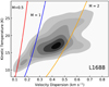 |
Fig. 7 Kinetic temperature and velocity dispersion in L1688, shown here as a normalised kernel density distribution. The contour levels are 0.1,0.2,0.3,0.5,0.7 and 0.9. The red, blue and orange lines represent Mach numbers of 0.5, 1 and 2, respectively. |
4.4 Identification of coherent cores
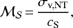
In order to study the change in kinetic temperature and velocity dispersion from cores to the surrounding material, wefirst identify what we consider as ‘coherent cores’. For this purpose, we use the sonic Mach number,  , which is defined as the ratio of the non-thermal velocity dispersion to the sound speed in the medium:
 (1)
(1)
where cS is the one-dimensional sound speed in the gas, given by :
 (2)
(2)
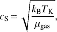
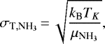
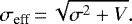
where kB is the Boltzmann’s constant, TK is the kinetic temperature in the region, and μgas is the average molecular mass (taken to be 2.37 amu, Kauffmann et al. 2008). The non-thermal component of the velocity dispersion is calculated by removing the thermal dispersion for the observed molecule (σT) from the total observed velocity dispersion (σv) :
 (3)
(3)
where σchan is the contribution due to the width of the channel. The thermal component of the dispersion observed in NH3 is:
 (4)
(4)
with  = 17 amu, being the mass of the ammonia molecule. For TK = 14 K, the thermal component (σT, NH3) is 0.082 km s−1.
When a Hann-like kernel is used in the spectrometer, the correction factor for the measured velocity dispersion is given by (see Leroy et al. 2016; Koch et al. 2018):
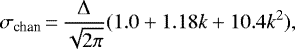 (5)
(5)
where Δ is the spectral resolution and k is dependent on the Hann-like function applied. In the case of the VEGAS spectrometer used in the GAS observations, k is 0.11, which corresponds to a correction term of:
 (6)
(6)
After applying this small correction, we obtain a typical non-thermal component of the velocity dispersion of σv,NT = 0.182km s−1, for σv = 0.2 km s−1.
In Fig. 7, it can be observed that a group of points lies below the line depicting a Mach number of 1, and a much larger distribution lies in the supersonic part of the plot. This separation is taken as the basis for separating the subsonic cores from the extended, more turbulent cloud. We first identify a mask with the regions in L1688 having a sonic Mach number of 1 or lower (similar to Pineda et al. 2010; Chen et al. 2019). Regions smaller than the beam size are removed from the mask. All the remaining regions are then considered as the ‘coherent cores’ in L1688.
Based on this definition, we identify 12 regions in L1688 as coherent cores (same as Paper I). These include:
-
five continuum cores, namely Oph-A, Oph-C, Oph-D, Oph-E and Oph-F. We identify two islands in Oph-A as coherent cores (Oph-A North, and Oph-A South), and consider them together as Oph-A;
-
one DCO+ core, Oph-B3 (Loren et al. 1990; Friesen et al. 2009);
-
two ‘coherent droplets’, L1688-d10 and L1688-d12, (Chen et al. 2019);
-
one prestellar core Oph-H-MM1 (Johnstone et al. 2004).
Apart from these previously identified cores6, we also identified three more subsonic regions : L1688-SR1 (south of Oph-B1), L1688-SR2 (three islands east of Oph-A) and L1688-SR3 (near the western edge of the map). These cores are shown in Fig. 8, along with the positions of Class 0/I and flat spectrum protostars in L1688 (Dunham et al. 2015). Following the classification of Class-0 and -I protostars in the region according to Enoch et al. (2009), we find no significant difference between the positions of Class 0/I protostars and those of flat spectrum protostars with respect to the coherent cores. The continuum cores Oph-B1 and Oph-B2 are not subsonic, as previously discussed (Sect. 4.3, see also : Friesen et al. 2009), and therefore, they are not considered as ‘coherent cores’ by our definition.
Because we use a larger beam (almost twice in size) compared to the GAS data, our definitions of the coherent boundaries are expected to vary slightly compared to other analyses carried out with the original data (e.g. Chen et al. 2019, which also applied more stringent criteria7 in their definition). However, comparison with Chen et al. (2019) shows that the overall coherent boundaries in the two works are consistent within one beam (1′).
Ladjelate et al. (2020) identifies a prestellar core at the position of SR1, and an unbound starless core at the position of SR3. SR1 and SR3 are associated with a local peak in NH3 integrated intensity. SR2 does not contain any bound core in Herschel data, nor does it show a local NH3 peak. However, as can be seen from our later results (presented in Sect. 5.5), the ambient cloud in the line of sight to the cores has a higher temperature compared to the gas in the core. However, in the computation of N(H2) from Herschel data, a single temperature was assumed for the entire line of sight. Therefore, it is possible that small clumps of over-densities at the position of coherent cores, which have a much lower temperature than that of the ambient cloud, will not be seen in the N(H2) maps. Without allowing for different temperatures in different parts of the cloud along the line of sight in the calculations of N(H2), we cannot dismiss the possibility of an over-density being associated with SR2.
In order to study the environment surrounding the coherent cores, we define two consecutive shells around each core. Shell-1 is defined as all the pixels around each coherent core, within a distance of one beam (the smallest resolved scale) from the boundary. Shell-2 is defined as all the pixels around shell-1 within one beam. This allows us to study the environment surrounding the cores in the two consecutive layers. The regions defined8 are displayed in Fig. 8.
As mentioned earlier, although considered as continuum cores, Oph-B1 and Oph-B2 are not coherent cores according to our definition. Being close to these two cores, the shells of Oph-B3 and L1688-SR1 might contain some high column density gas with supersonic velocity dispersions, produced by protostellar feedback, which is not representative of the cloud surrounding a coherent core. Therefore, we define a boundary roughly containing Oph-B1 and Oph-B2 based on column density (N(H2) > 2.1 × 1022 cm−2, shown in white dashed contours in Fig. 8), and remove the pixels inside this boundary from the shells of Oph-B3 and L1688-SR1 for all subsequent analyses.
 |
Fig. 8 Coherent cores and their immediate neighbourhood, as defined in Sect. 4.4, shown in the velocity dispersion map. The coherent cores, and the shell-1 and shell-2 regions are shown with blue, red, and green contours, respectively.The white dashed contour shows the boundary considered for continuum cores Oph-B1 and Oph-B2 (see Sect. 4.4 for details). The white stars show the positions of Class 0/I and flat-spectrum protostars in the cloud. The beam and the scale bar are shown in the bottom left and bottom right corners, respectively. |
 |
Fig. 9 Left: distribution of kinetic temperature and velocity dispersion for all the coherent cores and the shell-1 and shell-2 regions. Shells-1 and shells-2 are defined as two consecutive shells of width equal to one beam around the respective coherent cores. Each kernel density distribution was normalised to have a peak density of 1. The contours show normalised KDE levels of 0.1, 0.25, 0.4, 0.55, 0.7 and 0.85. Right: same as the left panel, but without the regions L1688-SR3, L1688-SR2, and Oph-A, and ignoring one beam at each star position. This is done to remove the effect of external heating, and possiblecontribution from prostellar feedback. |
5 Discussion
5.1 Transition from coherent cores to their immediate neighbourhood: a distribution analysis
We study the change in kinetic temperature and dispersion observed between the coherent cores and their surrounding environment(shell-1 and shell-2). The left panel of Fig. 9 shows the kernel density distribution of kinetic temperature with velocity dispersion for all the cores, and corresponding shell-1 and shell-2. The coherent cores are characterised by a kinetic temperature 3–7 K lower than shell-1 and shell-2. The velocity dispersion in the cores is also 0.2–0.4 km s−1 lower than in the shells. Compared to the change in TK and σv from core to shell-1, the values of the two parameters in shell-1 and shell-2 do not change as much. The kinetic temperatures of the two shells are within ≈2 K of each other, and the difference in dispersion is ≤ 0.1 km s−1.
The transition from the coherent cores to the surrounding molecular cloud in kinetic temperature is gradual, and there is no sudden jump, indicating that it changes smoothly from core to cloud at the angular resolution of the present work. By our definition of the cores, the transition in velocity dispersion at the core boundaries is sharp. The average kinetic temperature and velocity dispersion for the coherent cores are 12.107 ± 0.009 K and 0.1495 ± 0.0001 km s−1, respectively9 with a standard deviation of 3.2 K and 0.047 km s−1. Similarly, for the first shell, the average values are TK = 15.80 ± 0.01 K (std. dev. = 3.12 K) and σv = 0.3175 ± 0.0002 km s−1 (std. dev. = 0.127 km s−1); and for the second shell, TK = 18.11 ± 0.02 K (std. dev. = 3.5 K) and σv = 0.4176 ± 0.0004 km s−1 (std. dev. = 0.127 km s−1). We selected three roundish cores: Oph-E, Oph-H-MM1 and L1688-d12, and compared the radial profiles of velocity dispersion with those reported in Chen et al. (2019). We observed that σv inside these coherent cores lies inside the 1σ distribution of pixels in each distance bin equal to the beam size for the corresponding droplet in Chen et al. (2019). Furthermore, we also observed that the radial profiles showed similar shape as compared to those in Chen et al. (2019), up to shell-2. Therefore, we see similar radial profiles to those of Chen et al. (2019), even though we are using a larger beam. On average, we see a kinetic temperature difference of ≈4 K between core and shell-2, i.e. ≈2′ from core. Harju et al. (2017) observed a similar increase in kinetic temperature, ≈ 5 K, 2′ away from the centre of the starless core H-MM1 (see also Crapsi et al. 2007). This is consistent with the temperature structure of externally heated dense cores (e.g. Evans et al. 2001; Zucconi et al. 2001).
Assuming the gas to be completely molecular, so that NH = 2 × N(H2), and the relation between hydrogen column density and optical extinction to be NH (cm−2) ≈ 2.21 × 10²¹ AV (mag) (Güver & Özel 2009), we find that the average extinction through the cores is ≈16 mag. Through shell-1 and shell-2, the average extinctions are AV ≈ 13.16 and AV ≈ 11.2 mag, respectively. As we do not have the p-NH3 column density in the extended cloud (away from the cores), we fit the average spectra (see Sect. 5.2) of each core and their shells to get an idea of the average N(p-NH3) in the regions. From that analysis, we find that the average p-NH3 column density in the cores is ≈ (8.99 ± 0.08) × 1013 cm−2; and that in shell-1 and shell-2 are (5.2 ± 0.1) × 1013 cm−2 and (3.7 ± 0.1) × 1013 cm−2, respectively.
As mentioned in Sect. 4.3, the west part of L1688 is affected by a strong external radiation field, the effect of which can be clearly seen in the kinetic temperature map (Fig. 5). The regions Oph-A, L1688-SR3, and L1688-SR2 lie in the affected region of the cloud. To get a clearer view of the behaviour of kinetic temperature and velocity dispersion in the embedded cores (without the effect of the outside illumination), we omit the regions L1688-SR3, L1688-SR2, and Oph-A, as well as their neighbourhoods. In order to remove any possible contribution from prostellar feedback in the regions, we also mask one beam at the positions of known protostars (Dunham et al. 2015). The distribution of the remaining cores and the shells is shown in the right panel of Fig. 9. When the effects of external illumination, and possible contributions from protostellar feedback are masked, the average kinetic temperature in the cores drops (11.66 ± 0.01 K, std. dev. = 1.71 K). The change in σv is not as stark, with the average for the new distribution being 0.1487 ± 0.0001 km s−1 (std. dev. = 0.038 km s−1). Similarly, masking the heating by the external radiation removes the high kinetic temperature region in shells 1 and 2, reducing the average temperature to 14.68 ± 0.02 K (std. dev. = 1.9 K) and 17.37 ± 0.02 K (std. dev. = 2.1 K), respectively. By comparison, the spread in σv remains almost constant, and its average value is unchanged (within errors). Therefore, our results suggest that the external irradiation is not accompanied by turbulence injection in the neighbourhood of the cores.
 |
Fig. 10 Left panel: velocity dispersion in the core and the shells determined from average spectra in the respective core or shell. Shells-1 and shells-2 are defined as two consecutive shells of width equal to one beam around the respective coherent cores. Right panel: velocity dispersion in the shells relative to their respective cores. |
5.2 Transition from coherent cores to their immediate neighbourhood: analysis of individual cores
For the cores L1688-SR3, Oph-D, and d12, we have the kinetic temperature information for very few points in shells 1 and 2. The individual pixels in these shells do not have sufficient S/N for a good fit, and therefore direct determination of the kinetic temperature in the individual pixels is not possible. Moreover, TK could not be determined in some pixels in the outer shells of d10, L1688-SR2, Oph-A and Oph-F either. Therefore, to get a fair comparison of the temperatures in the cores, shells-1 and shells-2, we average the spectra in each of these regions. Stacking the spectra for a large number of points results in significantly reduced noise levels, and we have sufficient S/N to be able to fit these spectra and obtain the kinetic temperature for each region. With the low noise, we are also able to look at minor details in the spectra towards each core and shell. To avoid any possible line broadening due to averaging in a region with velocity gradients, we align the spectra at each pixel within a region before averaging. For this, we take the velocity at a pixel, determined from the one-component fit at that pixel, and using the channelShift function from module gridregion in the GAS pipeline10, we shift the spectra at that pixelby the corresponding number of channels. We then average the resultant spectra from all pixels inside a region, now essentially aligned at v = 0.
Figures 10 and 11 show the velocity dispersion and kinetic temperature, respectively, at each individual core and their respective neighbourhoods, determined from one-component fits to the averaged spectra in those regions. This gives us an idea of the change in the parameters as we move from core to shell-1, and then to shell-2. The left panel of Fig. 10 shows the velocity dispersions of each individual core, shell-1 and shell-2. The right panel shows the σv of the shells, relative to their corresponding cores. Similarly, Fig. 11 shows this relation for kinetic temperature.
Figure 10 shows that, as expected, the velocity dispersion increases from core to shell-1 for all cores. For most cores, the dispersion steadily increases outwards to shell-2. Oph-E is an exception to this, where σv decreases slightly in shell-2. It is clearly seen that for all the cores, the kinetic temperature steadily increases from the cores to shells 1 and 2. For d12, we see a slight drop in temperature from shell-1 to shell-2, but the difference is within the error margin, and therefore not significant. It can be again seen that the highest kinetic temperatures for cores, shell-1 and shell-2 are for the regions affected by the outside illumination (Oph-A, L1688-SR2 and L1688-SR3). The temperature rise from shell-1 to shell-2 for Oph-C is very drastic, as the second shell includes part of the cloud heated by the external radiation (see Fig. A.1 for reference).
We estimate the volume densities in the core, shell-1, and shell-2, with the Tex, TK, and τ measurements from the one-component fits using the following relation described in Foster et al. (2009):
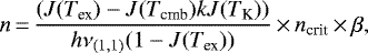 (7)
(7)
where Tcmb = 2.73 K, ncrit = 2 × 10⁴, k is the Boltzmann’s constant, h is the Planck’s constant, β is the escape probability estimated as β = (1 − e−τ)∕τ, and
 (8)
(8)
We find the cores to have a mean density of 1.66 ± 0.09 × 105 cm−3. Shell-1 and shell-2 have similar densities: 1.5 ± 0.1 × 10⁵ and 1.4 ± 0.2 × 105 cm−3, respectively11. The densities in all of these three regions are more than an order of magnitude higher than the average density of the cloud traced by NH3, calculated using the N(H2) estimate from Herschel (~4 × 103cm−3, see Sect. 2.1). It should be noted that the density estimate from Foster et al. (2009) uses measurements with NH3, which traces a higher density than dust continuum. Therefore, by design, the Foster et al. (2009) estimate is mainly sensitive to higher density regions, whereas the Herschel continuum measurements refer to a significantly larger volume (as dust is much more extended than NH3). Also, the Herschel column density maps are obtained assuming a single line-of-sight dust temperature, which might create discrepancies in the N(H2) estimate, especially towards the cores, which are much colder than the surrounding gas. Therefore, a systematic difference in the two density estimates (using NH3, and from the N(H2) map) is expected.
 |
Fig. 11 Left panel: kinetic temperature in core and the shells, determined from average spectra in the respective core or shell. Shells-1 and shells-2 are defined as two consecutive shells of width equal to one beam around the respective coherent cores. Right panel: kinetic temperature in the shells relative to their respective cores. |
5.3 Comparison of kinetic temperature with dust temperature
In Fig. 12, we show the map of the difference between the kinetic temperature derived using NH3 and the dust temperature derived from Herschel. The blue region in the map shows the gas with kinetic temperatureless than dust temperature, and the red part shows the region in L1688 with kinetic temperature higher than dust temperature. Gas and dust are expected to be effectively coupled only at densities above 104.5 cm−3 (Goldsmith 2001; Galli et al. 2002). The average density in L1688 is lower than 104 cm−3 (Sect. 2.1) and therefore gas–dust coupling is not achieved in this cloud (except in the core regions and their neighbourhoods).
Although NH3 emission in L1688 is extended, the comparison with the dust temperature indicates that NH3 is not tracing the larger scale molecular cloud traced by the dust emission (or by low-density tracers such as CO). Instead, it is likely tracing the inner region of the cloud (at Av > 10 mag), where NH3 is abundant and its inversion transitions can be excited. The coherent cores have a lower kinetic temperature than dust temperatures, even though their identification is done only using the kinematical information (σv). This is expected, because the NH3 emission towards the cores is dominated by the inner dense, cold core material; whereas the dust temperature is representative of the temperatureof the foreground, outer part of the cloud. On average, the kinetic temperature in the coherent cores is 1.8 K lower than the dust temperature. In the two shells surrounding the cores, the situation is reversed. In shell-1, the kinetic temperature is marginally higher (≈0.3 K) than the dust temperature, and in shell-2, the difference is even stronger, TK - Tdust ≈ 1.8 K. The gas towards the western edge, which is affected by the strong external radiation (defined as the region to the right of the vertical dotted line shown in Fig. 3), shows ammonia at a temperature that is ≈5 K higher than the dust temperature. This region is illuminated by a far-ultraviolet (FUV) field of ~400 G0 (Habart et al. 2003). Therefore, the gas temperature in this region is significantly higher than the dust temperature, as expected in a dense region with high external illumination (Koumpia et al. 2015), and as gas–dust coupling is not achieved at those densities.
5.4 Ammonia abundance
To see how the ammonia abundance varies going from the cores to the surrounding cloud, we separate the points in the coherent cores and the shells. It can be seen from Fig. 6, that we are not able to obtain a much extended map for the p-NH3 column density. Consequently, we have too few points in shell-2 of the cores for a meaningful analysis. Therefore, we limit our analysis of NH3 abundance to only the cores and shell-1. As mentioned in Sect. 3.1, in this work we focus on the column density of only para-ammonia. We do not attempt to convert this into the total NH3 column density because the ortho-to-para ratio is unknown.
Figure 13 shows the distribution of N(p-NH3) with N(H2), inside the cores (left panel) and shell-1 (right panel). We note that the plots only show the pixels, for which a good determination of N(p-NH3) was possible. To clearly show the distribution of a large number of points, we plot the KDE instead of the individual data points in the plots (the calculation of KDE distribution from the data is explained in Sect. 4.3). The error in p-NH3 column density is considered in the calculation of the KDE.
To get an estimate of the para-ammonia abundance in the cores and shell-1, we fit a straight line of the form y = mx + c to each data set. The slope of the line, m, gives us the fractional para-ammonia abundance, X(p -NH3) = N(p-NH3)∕N(H2), in the region. We use curve_fit from the python package scipy to obtain the best linear fit. We take into account the error in our calculation of N(p-NH3) in fitting this data. However, as the error associated with the H2 column density was not available in the Herschel public archive, we do not incorporate any error in the x-axis for the fit.
The model in the core is a good fit to the data. The fit in shell-1 is slightly offset from the peak due to the presence of a small number of high N(p-NH3) points. However, the fit still provides a good constraint on the slope, which is the parameter of interest. From this analysis, we report an average para-ammonia fractional abundance (with respect to H2) of 4.2 ± 0.2 × 10⁻⁹ in the coherent cores, and 1.4 ± 0.1 × 10⁻⁹ in shell-1. Therefore, the para-ammonia abundance drops by a factor of three from the cores to their immediate surroundings. The p-NH3 abundance within the coherentcores reported here is comparable to that in L1544, as found by Tafalla et al. (2002), Crapsi et al. (2007), and Caselli et al. (2017), which is ≈ 4 × 10⁻⁹. Crapsi et al. (2007) also report a similar drop in abundance for a similar distance outside the core in L1544. These latter authors report an abundance of ≈2 × 10⁻⁹ at a distance ~10 000 au. This is comparable to the abundance we report for shell-1, which is at a similar distance (~10 000 au) from the cores in our study12.
 |
Fig. 12 Map of the difference between kinetic temperature (from NH3) and dust temperature (from Herschel). The black stars show the positions of known protostars in the region. The solid black contours show the coherent cores in the region (see Sect. 4.4). The beam and the scale bar are shown in the bottom-left and bottom-right corners, respectively. |
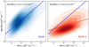 |
Fig. 13 Kernel density estimate representation of the distribution of p-NH3 column density with N(H2) in the cores (in red) and shell-1 (in blue), as defined in Sect. 4.4 and shown in Fig. 8. The straight lines show the best linear fit to the data in the corresponding region. For comparison between the regions, the linear fit to the data in the cores (red line) is also shown in the plot for shell-1. The slopes of the linear fits indicate the fractional p-NH3 abundance (with respect to H2) in the region, which is shown in the top-left corner. |
5.5 Presence of a second component : comparison with Paper I results
From the fits and corresponding residuals to the average spectra towards all the cores and most of the shells (Figs. B.1–B.12), we see that the single component fits do not recover all the flux. This indicates the presence of a second component in these spectra. In Paper I, we analysed the dual-component nature of the spectra towards the cores. It was shown that a faint supersonic component is present along with the narrow core component, towards all cores. We suggested that the narrow component is representative of the subsonic core, and the broad component traces the foreground cloud next to the cores. Here, we extend that analysis to shell-1 and shell-2 around the coherent cores, and study how the two components change going from the cores to their shells.
Similar to Paper I, we use the Akaike information criterion (AIC), which determines if the quality of the model improves significantly, considering the increase in the number of parameters used. We find that for all the regions, the two-component fit is a better model to the spectra. However, with a closer look at the spectra, we see that for shell-2 of d12, and shell-1 of SR3, one of the components fit by the model has very large σv (>1 km s−1), and is very faint (peak TMB, (1,1) ≈ 10 mK, which is comparable to, or lower than the noise in the spectrum). Therefore, we do not have reliable constraints for the fits to these components, and so we do not consider them for further analysis.
Extending the definition of the two components used in Paper I, we refer to the two components as ‘narrow’ and ‘broad’ based on their velocity dispersion. However, it should be noted that unlike towards the cores (in Paper I), the narrow components in the shells, especially shell-2, are not always subsonic. In this paper, our distinction of the components is merely based on the velocity dispersion, in order to be able to track the transition of each component from core to shell-2.
Figure 14 shows the variation of the peak main beam brightness temperature of the (1,1) across cores and shells for the narrow component (left panel) and the broad component (right panel). It can be seen that the intensity of the narrow component decreases sharply from core to shell-1, and less so from shell-1 to shell-2. In comparison, the intensity of the broad component remains largely constant for all three regions. This result agrees with the conclusions of Paper I, in that the narrow component is the core component, and the broad component is a single cloud component representative of the surrounding cloud. This figure also shows that the single component fit results would be skewed towards the narrow component in the core. The flux is dominated by the broad components in shell-2 because of the larger width, as the intensities are similar to those of the narrow components. For shell-1, neither component is clearly dominant.
The variation of velocity dispersion and kinetic temperature from the cores to the shells for the two components, are shown in Figs. 15 and 16, respectively. It can clearly be seen from Fig. 15 that the narrow component becomes more turbulent further away from the cores. The broad cloud component does not show any clear trend and is mostly invariant. The narrow component, even in shell-2, has lower σv than the broad component towards the cores. This again agrees with the interpretation of Paper I, in that the narrow component traces the subsonic core, and the broad component traces the more turbulent surrounding cloud.
For the kinetic temperature, we do not see a clear trend in either of the two components (Fig. 16). It can be seen that the narrow component is slightly colder towards the cores compared to the shells. In general, the narrow component is at a lower temperature than the broad component. In shell-2 of Oph-C, the (2,2) line could not be fit for the broad component, and therefore, the kinetic temperature of that component is not well defined. Hence, shell-2 of Oph-C is omitted from Fig. 16 (for the broad component).
Figure 16 shows that for H-MM1, the kinetic temperature of the narrow component shows an unusual trend, in that TK in shell-2 seems to be ≈20 K higher than that in the core. A look at the spectra (Fig. B.7) reveals that the relative positions of the narrow and broad component seem to switch from core and shell-1, to shell-2. The narrow component in shell-2 seems to be brighter in (2,2) than in shell-1. These unexpected behaviours could be explained by the relatively small change in AIC in the two-component fit, from the one-component fit (see Table C.1). As mentioned in Appendix E of Paper I, the physical properties derived from two-component fit are not well constrained, for small ΔAIC (= AIC1-comp −AIC2-comp). In particular, for H-MM1, we find that more restrictions (e.g., not allowing the two components to switch their relative positions) results in a different two-component fit, with only a slightly smaller ΔAIC (= 27). This alternate fit (Fig. B.13) indicates that there is no subsonic component in shell-2, but rather, two supersonic components (σv ≈ 0.28 km s−1 for both). Therefore, as already mentioned in Paper I, we need to be cautious while considering the regions with low ΔAIC values, and need to inspect the fits to the spectra carefully.
In Paper I, we reported that the ambient cloud in L1688 (considered to be represented by the rectangular box shown in Fig. 2) shows two supersonic components, with a small relative velocity. We suggested that a collision between these two cloud components might result in a local density increase, where the merging of the two broad components locally produces the narrow feature, following a corresponding dissipation of turbulence; thus creating the observed coherent cores with subsonic line widths. The gradual decrease in the dispersion of the narrow component, from shell-2 to core is congruent with this hypothesis.
Figure 17 shows the temperature of each coherent core (narrow component) as a function of the relative velocity between the two components towards the core. Here, we have not considered Oph-A, SR2, and SR3 to remove any possible contribution of the external radiation from the west. A general trend can be seen, with the core temperature increasing with the relative velocity of the two components. This might suggest that collision between the two components is responsible for a local temperature increase. However, owing to our relatively large beam, we cannot conclusively comment on the presence of local shocks (e.g. Pon et al. 2012), and would require higher resolution data in the region and observations in shock tracers to confirm or rule out this possibility.
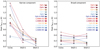 |
Fig. 14 Left panel: peak main beam brightness temperature of (1,1), for the narrow component in the cores, shells-1, and shells-2. Shell-1 and shell-2 are defined as two consecutive shells of width equal to one beam around the respective coherent cores. Right panel: same variance, but for the broad component. We note that as we do not consider the two-component fit to shell-1of SR3 (see Sect. 5.5), the values for the core and shell-2 are connected by a dashed line. |
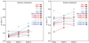 |
Fig. 15 Left panel: velocity dispersion of the narrow component in the cores, shells-1 and shells-2. Shells-1 and shells-2 are defined as two consecutive shells of width equal to one beam around the respective coherent cores. The black-dotted line shows the velocity dispersion with
|

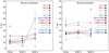 |
Fig. 16 Left panel: kinetic temperature of the narrow component in the cores, shells-1 and shells-2. Shells-1 and shells-2 are defined as two consecutive shells of width equal to one beam around the respective coherent cores. Right panel: same variation, but for the broad component. We note that as we do not consider the two-component fit to shell-1 of SR3 (see Sect. 5.5), the values for the core and shell-2 are connected by a dashed line. |
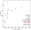 |
Fig. 17 Kinetic temperature of the core (narrow) component, against the relative velocity between the core (narrow) component and the cloud (broad) component, towards each core. Oph-A, SR2, and SR3 are affected by the external illuminationand are therefore not considered in this analysis. |
5.6 Evidence of a subsonic component beyond previously identified coherent zones
The subsonic component seen in the cores is also detected in shell-1 for 10 out of the 12 coherent cores (except Oph-E, where there is no subsonic component in shell-1, and SR3, where the two-component fit in shell-1 of SR3 is not well constrained; see Sect. 5.5). Furthermore, in five regions (Oph-A, Oph-D, H-MM1, SR1 and SR2), the component with subsonic turbulence can be detected even in shell-2. This suggests that the subsonic component extends well beyond the typical boundary of the coherent cores, albeit much fainter in intensity (approximately one-fifth of the peak intensity in NH3 (1,1)) than that towards the cores. This suggests that the transition to coherence is not sharp, as previously reported (e.g. Pineda et al. 2010; Friesen et al. 2017; Chen et al. 2019), but rather gradual. The sharp transition to coherence observed by Pineda et al. (2010) was within a 0.04 pc scale, which is very similar to our spatial resolution (1′ at ≈138 pc). It is likely that the transition observed by Pineda et al. (2010) in B5 was the transition between the narrow and the broad component. Due to the poorer sensitivity of the data, the broad component towards the core and the subsonic component outside the core boundary were not detected in their work. With averaged spectra, we are able to detect the two components towards the cores and the shells, and we observe that the coherent cores in Ophiuchus are indeed more extended than previously found with a one-component fit.
It should be noted that due to the lack of sensitivity, even with the smoothed data, we are not able to detect the broad component across the entire region; and the two-component analysis is only possible with the stacked spectra in the coherent cores and the shells. Therefore, with our current sensitivity, we cannot use the narrow component to define the coherent core, which would be the ideal case, as we do not have a map of the narrow (or broad) component. We are therefore limited by the sensitivity to using the one-component fit, to define the coherent boundaries, as is the case in the existing literature. Our present results indicate that with more sensitive data, which would allow for a two-component fit, the coherent boundary could be improved.
We also observe that the core component smoothly broadens up to a supersonic velocity dispersion towards some cores, but the dispersion still does not reach that of the broad component at the corresponding position (see Fig. 15). Although the value of the broad component could be interpreted as the level of turbulence outside the core, it is more likely that the larger velocity dispersion is due to a change in the scale traced along the line of sight, which could include large-scale velocity structure.
5.7 Turbulence–size relation
We observe the subsonic component extending outside the typical boundary of the coherent cores. We also observe this component gradually broadening outwards from the cores (Fig. 15). Therefore, we looked at the relation between the turbulence (non-thermal velocity dispersion) in the component and the size of the regions. We define the equivalent radius (req) for each region as  , where A is the area inside that region (core, shell-1 or shell-2).
As we could only detect the subsonic component outside the typical coherent core using stacked spectra in the shells with our current data, we only have three data-points for each core with which to fit for the turbulence–size relation. Moreover, the σv,NT for shell-2 often has relatively large errors (see Table C.1). Therefore, with the present sensitivity, we cannot obtain a reliable turbulence–size relation for each core separately, and so, we only fit an average relation considering all cores together. Figure 18 shows the turbulence in the narrow component towards each coherent core, shell-1 and shell-2 as a function of the respective equivalent radii.
We fit a power law, σv,NT = a rb, to the whole sample using the uncertainty in the derived non-thermal velocity dispersion with emcee (Foreman-Mackey et al. 2013). As we fit for an average relation for all the cores, we allow for a Gaussian intrinsic scatter term (with variance V) to the model, to account for the spread due to considering multiple cores. In the calculation of the likelihood parameter, the uncertainty in the model, σ, is then replaced by
 (9)
(9)
We use uniform priors for the exponent (b) and the constant (a) with a range that includes both tails of the individual posterior probability distributions. We then sample the distribution using emcee with 32 walkers in a 2D Gaussian around the maximum-likelihood result, and run 5000 steps of Markov chain Monte Carlo (MCMC). With this, we obtain an auto-correlation time of ≈ 40 steps. We discard the first 200 steps to avoid effects of initialisation, and trim the distribution by half the auto-correlation time (20 steps). From this analysis, we determine the best fit to the data as
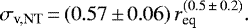 (10)
(10)
The derived exponent is consistent with the one reported by Caselli & Myers (1995) within the error bar. However, in that study, the authors use a sample of mixed tracers, including 13CO. Our results focus this relation to a narrow range of small-scale structures, down to ≈ 0.02 pc. The similarity of the exponent with the results from Caselli & Myers (1995) suggest that the turbulence–size relation remains approximately the same on scales closer to the core centre. Chen et al. (2020) also observed similar exponents in line-width–size relations for Phase-I and -II cores in synthetic observations13.
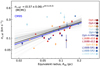 |
Fig. 18 Non-thermal velocity dispersions in the narrow component for each core, shell-1, and shell-2 as a function of their equivalent radii. The grey lines show the power-law fits for the range of parameters obtained from a MCMC fit, and the black line shows the best-fit model. The blue line shows the turbulence–size relation from Caselli & Myers (1995) for low-mass cores. |
6 Conclusions
We present a new analysis of the GAS DR1 data with GBT towards L1688 smoothed to 1′ resolution. Our results can be summarised as follows:
- 1.
For the first time, we obtain substantially extended kinetic temperature and velocity dispersion maps, covering 65% and 73.4% of the observed area, respectively, including dense cores and the surrounding molecular cloud, using the same density tracer. This ensures continuity in the physical properties from core to cloud.
- 2.
We identify 12 coherent cores in L1688 (same as Paper I), including 3 previously unidentified subsonic regions, SR1, SR2 andSR3.
- 3.
Using a one-component fit to the data, we observe that both the kinetic temperature and the velocity dispersion gradually increase outwards from the coherent cores. On average, the kinetic temperature 1′ (≈8000 au) and 2′ (≈16 000 au) away from the core boundary is approximately 4 K and 6 K higher than the core temperature. Similarly, the velocity dispersion in these regions is 0.15 and 0.25 km s−1 higher than that in the core, respectively.
- 4.
We find that the external illumination at the western edge of the cloud is not accompanied by turbulence injection.
- 5.
The kinetic temperature towards the coherent cores is, on average, ≈1.8 K lower than the dust temperature. Outside the cores, the kinetic temperature of the gas is higher than the dust temperature.
- 6.
We find an average para-ammonia fractional abundance (with respect to H2) of 4.2 ± 0.2 × 10⁻⁹ in the coherent cores, and 1.4 ± 0.1 × 10⁻⁹, at 1′ from the core. Previous works report a similar abundance within the core for L1544, and a similar drop in abundance for a similar distance outside the core.
- 7.
By stacking the spectra towards the cores and their neighbourhoods, we are able to detect two velocity components, one narrow and one broad, superposed in velocity. For most cores, we observe that the component with subsonic turbulence is extended beyond the previously identified coherent regions. This suggests that the transition to coherence is gradual, in contrast to previous results. We observe that the subsonic component towards the cores becomes fainter and broader outwards, with a turbulence–size relation of
 , with b = 0.5 ± 0.2, similar to what was found in other low-mass dense cores using multiple molecular tracers.
 - 8.
In contrast, the broad component shows near-constant intensity and dispersion towards core and cloud. This supports our conclusions from Paper I of the broad component tracing material across the larger scale cloud seen with ammonia.
- 9.
We observe that on average the cores with higher velocities relative to the surrounding cloud show higher temperatures. With higher resolution maps of the region and with adequate sensitivity, it would be possible to determine whether or not there are any local shocks around the coherent cores.
Acknowledgements
S.C., J.E.P., and P.C. acknowledge the support by the Max Planck Society. This material is based upon work supported by the Green Bank Observatory which is a major facility funded by the National Science Foundation operated by Associated Universities, Inc. A.C.-T. acknowledges the support from MINECO projects AYA2016-79006-P and PID2019-108765GB-I00. AP acknowledges the support from the Russian Ministry of Science and Higher Education via the State Assignment Project FEUZ-2020-0038. A.P. is a member of the Max Planck Partner Group at the Ural Federal University.
Appendix A Selection of cores, and shells
Figures A.1 and A.2 show the cores, with shell-1 and shell-2 around each of them, similar to Fig. 8, but with kinetic temperature and sonic Mach number as the background colour-scale.
 |
Fig. A.1 Coherent cores and shells-1 and -2, as defined in Sect. 4.4, are shown on the kinetic temperaturemap, with blue, red and green contours, respectively. The white stars show the positions of Class 0/I and flat-spectrum protostars in the cloud. The white dashed contour shows a rough boundary for Oph-B1 and Oph-B2 (see Sect. 4.4). The white dotted line roughly separates the dark cloud to the left from the molecular material affected by the external illumination to the right. |
Appendix B Averaged spectra in the cores, shell-1 and shell-2
Figures B.1–B.12 shows the average spectra in the respective coherent cores, used in Sect. 5.2. The final model determined by the fit is overlaid (in green) on the spectra.
Figure B.13 shows an alternate two-component fit to shell-2 of H-MM1. Here, we have restricted the relative positions of the narrow and the broad components, so that the narrow component is always at a higher velocity than the broad component (Sect. 5.5).
 |
Fig. B.1 Top panels: average NH3 (1,1) and (2,2) spectra of Oph-A core, shell-1 and shell-2 with a one-component fit. Bottom panels: same spectra, but with a two-component fit (green). The narrow (red) and broad (blue) components are also shown separately. |
Appendix C Fit parameters for average spectra
In Table C.1, we present the kinetic temperature, velocity dispersion and p-NH3 column densities for the cores and shells-1 and -2, from one-component fits and two-component fits to the average spectra in the respective regions. We also show the improvement in the fit (as change in AIC value) from one- to two-component fit, and the noise level, for each spectrum.
Best-fit parameters for one- and two-component fits in cores and shells.
References
- André, P., Men’shchikov, A., Bontemps, S., et al. 2010, A&A, 518, L102 [NASA ADS] [CrossRef] [EDP Sciences] [Google Scholar]
- Barranco, J. A., & Goodman, A. A. 1998, ApJ, 504, 207 [Google Scholar]
- Bergin, E. A., & Langer, W. D. 1997, ApJ, 486, 316 [Google Scholar]
- Caselli, P., & Myers, P. C. 1995, ApJ, 446, 665 [Google Scholar]
- Caselli, P., Bizzocchi, L., Keto, E., et al. 2017, A&A, 603, L1 [NASA ADS] [CrossRef] [EDP Sciences] [Google Scholar]
- Chen, H. H.-H., Pineda, J. E., Goodman, A. A., et al. 2019, ApJ, 877, 93 [Google Scholar]
- Chen, H. H.-H., Offner, S. S. R., Pineda, J. E., et al. 2020, ApJ, submitted [arXiv:2006.07325] [Google Scholar]
- Choudhury, S., Pineda, J. E., Caselli, P., et al. 2020, A&A, 640, L6 [EDP Sciences] [Google Scholar]
- Crapsi, A., Caselli, P., Walmsley, M. C., & Tafalla, M. 2007, A&A, 470, 221 [NASA ADS] [CrossRef] [EDP Sciences] [Google Scholar]
- Di Francesco, J., André, P., & Myers, P. C. 2004, ApJ, 617, 425 [NASA ADS] [CrossRef] [Google Scholar]
- Dunham, M. M., Allen, L. E., Evans, Neal J., I., et al. 2015, ApJS, 220, 11 [Google Scholar]
- Enoch, M. L., Evans, N. J., I., Sargent, A. I., & Glenn, J. 2009, ApJ, 692, 973 [Google Scholar]
- Evans, N. J., I., Rawlings, J. M. C., Shirley, Y. L., & Mundy, L. G. 2001, ApJ, 557, 193 [Google Scholar]
- Foreman-Mackey, D., Hogg, D. W., Lang, D., & Goodman, J. 2013, PASP, 125, 306 [Google Scholar]
- Foster, J. B., Rosolowsky, E. W., Kauffmann, J., et al. 2009, ApJ, 696, 298 [Google Scholar]
- Friesen, R. K., Di Francesco, J., Shirley, Y. L., & Myers, P. C. 2009, ApJ, 697, 1457 [Google Scholar]
- Friesen, R. K., Pineda, J. E., co-PIs, et al. 2017, ApJ, 843, 63 [NASA ADS] [CrossRef] [Google Scholar]
- Gaia Collaboration 2018, VizieR Online Data Catalog: I/345 [Google Scholar]
- Galli, D., Walmsley, M., & Gonçalves, J. 2002, A&A, 394, 275 [NASA ADS] [CrossRef] [EDP Sciences] [Google Scholar]
- Ginsburg, A., & Mirocha, J. 2011, PySpecKit: Python Spectroscopic Toolkit [Google Scholar]
- Goldsmith, P. F. 2001, ApJ, 557, 736 [NASA ADS] [CrossRef] [MathSciNet] [Google Scholar]
- Goodman, A. A., Barranco, J. A., Wilner, D. J., & Heyer, M. H. 1998, ApJ, 504, 223 [Google Scholar]
- Güver, T., & Özel, F. 2009, MNRAS, 400, 2050 [Google Scholar]
- Habart, E., Boulanger, F., Verstraete, L., et al. 2003, A&A, 397, 623 [NASA ADS] [CrossRef] [EDP Sciences] [Google Scholar]
- Habing, H. J. 1968, Bull. Astron. Inst. Netherlands, 19, 421 [Google Scholar]
- Harju, J., Daniel, F., Sipilä, O., et al. 2017, A&A, 600, A61 [NASA ADS] [CrossRef] [EDP Sciences] [Google Scholar]
- Hollenbach, D. J., & Tielens, A. G. G. M. 1999, Rev. Mod. Phys., 71, 173 [Google Scholar]
- Houk, N., & Smith-Moore, M. 1988, Michigan Catalogue of Two-dimensional Spectral Types for the HD Stars. Volume 4, Declinations -26°.0 to -12°.0. [Google Scholar]
- Ivlev, A. V., Silsbee, K., Sipilä, O., & Caselli, P. 2019, ApJ, 884, 176 [Google Scholar]
- Johnstone, D., Di Francesco, J., & Kirk, H. 2004, ApJ, 611, L45 [Google Scholar]
- Kamazaki, T., Saito, M., Hirano, N., Umemoto, T., & Kawabe, R. 2003, ApJ, 584, 357 [Google Scholar]
- Kauffmann, J., Bertoldi, F., Bourke, T. L., Evans, N. J., I., & Lee, C. W. 2008, A&A, 487, 993 [NASA ADS] [CrossRef] [EDP Sciences] [Google Scholar]
- Koch, E., Rosolowsky, E., & Leroy, A. K. 2018, Res. Notes AAS, 2, 220 [Google Scholar]
- Koumpia, E., Harvey, P. M., Ossenkopf, V., et al. 2015, A&A, 580, A68 [NASA ADS] [CrossRef] [EDP Sciences] [Google Scholar]
- Ladjelate, B., André, P., Könyves, V., & Men’shchikov, A. 2016, IAU Symp., 315, E46 [Google Scholar]
- Ladjelate, B., André, P., Könyves, V., et al. 2020, A&A 638, A74 [CrossRef] [EDP Sciences] [Google Scholar]
- Launhardt, R., Stutz, A. M., Schmiedeke, A., et al. 2013, A&A, 551, A98 [NASA ADS] [CrossRef] [EDP Sciences] [Google Scholar]
- Leroy, A. K., Hughes, A., Schruba, A., et al. 2016, ApJ, 831, 16 [Google Scholar]
- Loren, R. B., Wootten, A., & Wilking, B. A. 1990, ApJ, 365, 269 [NASA ADS] [CrossRef] [Google Scholar]
- Lovas, F. J., Bass, J. E., Dragoset, R. A., & Olsen, K. J. 2009, NIST Recommended Rest Frequencies for Observed Interstellar Molecular Microwave Transitions - 2009 Revision, (version 3.0), http://physics.nist.gov/restfreq, [Online; accessed 15-May-2020] [Google Scholar]
- Markwardt, C. B. 2009, ASP Conf. Ser., 411, 251 [Google Scholar]
- Motte, F., Andre, P., & Neri, R. 1998, A&A, 336, 150 [NASA ADS] [Google Scholar]
- Ortiz-León, G. N., Loinard, L., Dzib, S. A., et al. 2018, ApJ, 869, L33 [Google Scholar]
- Pagani, L., Bacmann, A., Cabrit, S., & Vastel, C. 2007, A&A, 467, 179 [NASA ADS] [CrossRef] [EDP Sciences] [Google Scholar]
- Pineda, J. E., Goodman, A. A., Arce, H. G., et al. 2010, ApJ, 712, L116 [Google Scholar]
- Pon, A., Johnstone, D., & Kaufman, M. J. 2012, ApJ, 748, 25 [Google Scholar]
- Scott, D. W. 1992, Multivariate Density Estimation: Theory, Practice, and Visualization (New York: John Wiley & Sons) [Google Scholar]
- Tafalla, M., Myers, P. C., Caselli, P., Walmsley, C. M., & Comito, C. 2002, ApJ, 569, 815 [Google Scholar]
- White, G. J., Drabek-Maunder, E., Rosolowsky, E., et al. 2015, MNRAS, 447, 1996 [Google Scholar]
- Young, K. E., Lee, J.-E., Evans, Neal J., I., Goldsmith, P. F., & Doty, S. D. 2004, ApJ, 614, 252 [Google Scholar]
- Zucconi, A., Walmsley, C. M., & Galli, D. 2001, A&A, 376, 650 [NASA ADS] [CrossRef] [EDP Sciences] [Google Scholar]
To compare to the total NH3 column densities reported in other works, an easy conversion is to multiply N(p-NH3) by 2, if the ortho-to-para ratio is assumed to be the LTE value of unity.
Although this threshold is below the noise level (≈ one-quarter), it was chosen because it significantly recovered the flux in the model.
We observe that typically for τ (1,1) < 0.12, it is difficult to constrain Tex and therefore the ammonia column densities.
Definition of G0 from Hollenbach & Tielens (1999): G0 represents the unit of an average interstellar flux of 1.6 erg cm−2 s−1 in the energy range 6–13.6 eV (Habing 1968).
Oph-B3, Oph-D and H-MM1 are also identified as L1688-c4, L1688-d11 and L1688-d9, respectively, in Chen et al. (2019). The two structures that we identify as Oph-A are likely associated with Oph-A-N2 and Oph-A-N6, as identified in N2 H+ by Di Francesco et al. (2004).
Chen et al. (2019) had further requirements for the coherent regions to be identified as ‘droplets’ (such as associated local maxima in peak NH3 (1,1) intensity and N(H2), and relatively smooth vLSR distribution inside), whereas we consider the sonic Mach number as the only criterion.
For most cases, the shells of different cores have little to no overlap. For L1688-d10 and H-MM1, there would have been some overlap with the shell definitions, but we avoid this overlap by restricting the boundaries of respective shells-2, as can be seen in Fig. 8.
All the averages reported in this section are weighted averages, with associated error on the weighted average.
Non-weighted averages.
These studies report the total ammonia abundance (X(NH3)). We convert this to X(p-NH3) for comparison, using an ortho-para ratio of unity, as assumed in these studies.
It should be noted that Chen et al. (2020) considered σv in their relation. For comparison with their work, we calculated the relation (10) for σv.
All Tables
All Figures
|
Fig. 1 Integrated intensity maps of NH3 (1,1) (top) and (2,2) (bottom) lines. For NH3 (1,1), the contour levels indicate 15σ,30σ, and 45σ, and for NH3 (2,2), contours are shown for 6σ,12σ, and 18σ; where σ is the median error in emitted intensity calculated from the signal-free spectral range in each pixel and converted to the error in integrated intensity. The moment maps were improved by considering only the spectral range containing emission, as described in Sect. 4.1. The 1′ beam, which the data was convolved to, is shown in green in the bottom-left corner, and the scale bar is shown in the bottom-right corner. |
| In the text | |
|
Fig. 2 N(H2) in L1688, taken from Herschel Gould Belt Survey archive. Positions of the continuum cores reported in Motte et al. (1998) are indicated by arrows. The dashed rectangle shows the area used to calculate mean cloud properties (see Sect. 4.3). The solid black contours show the coherent cores in the region (described later in Sect. 4.4). The 1′ beam, which the data was convolved to, is shown in orange in the bottom-left corner, and the scale bar is shown in the bottom-right corner. |
| In the text | |
|
Fig. 3 Dust temperature in L1688, taken from Herschel Gould Belt Survey archive. The solid white contours show the coherent cores in the region (described later in Sect. 4.4). The vertical dotted line roughly separates the dark cloud (to the left of the line) from the molecular material affected by the external illumination, due to irradiation from HD147889 (Habart et al. 2003). The 1′ beam, which the data was convolved to, is shown in green in the bottom-left corner, and the scale bar is shown in the bottom-right corner. |
| In the text | |
|
Fig. 4 Centroid velocity (top panel) and velocity dispersion (bottom panel) in L1688. The solid black contours in the top panel and solid blue contours in the bottom panel show the coherent cores in the region (described later in Sect. 4.4). The black (top panel) and white (bottom panel) stars show the positions of Class 0/I and flat-spectrum protostars (Dunham et al. 2015). The beam is shown in green in the bottom-left corner, and the scale bar is shown in the bottom-right corner. |
| In the text | |
|
Fig. 5 Kinetic temperature in L1688. The solid blue contours show the coherent cores in the region (described later in Sect. 4.4). The white stars show the positions of Class 0/I and flat-spectrum protostars. To see the difference between the part of the cloud affected by the external radiation, and the dark cloud further away from the illuminationsource, we consider a vertical boundary, as shown. The beam is shown in green in the bottom-left corner, and the scale bar is shown in the bottom-right corner. |
| In the text | |
|
Fig. 6 p-NH3 column density in L1688. The solid white contours show the coherent cores in the region (described later in Sect. 4.4). The black stars show the positions of Class 0/I and flat-spectrum protostars. The beam is shown in green in the bottom-left corner, and the scale bar is shown in the bottom-right corner. |
| In the text | |
|
Fig. 7 Kinetic temperature and velocity dispersion in L1688, shown here as a normalised kernel density distribution. The contour levels are 0.1,0.2,0.3,0.5,0.7 and 0.9. The red, blue and orange lines represent Mach numbers of 0.5, 1 and 2, respectively. |
| In the text | |
|
Fig. 8 Coherent cores and their immediate neighbourhood, as defined in Sect. 4.4, shown in the velocity dispersion map. The coherent cores, and the shell-1 and shell-2 regions are shown with blue, red, and green contours, respectively.The white dashed contour shows the boundary considered for continuum cores Oph-B1 and Oph-B2 (see Sect. 4.4 for details). The white stars show the positions of Class 0/I and flat-spectrum protostars in the cloud. The beam and the scale bar are shown in the bottom left and bottom right corners, respectively. |
| In the text | |
|
Fig. 9 Left: distribution of kinetic temperature and velocity dispersion for all the coherent cores and the shell-1 and shell-2 regions. Shells-1 and shells-2 are defined as two consecutive shells of width equal to one beam around the respective coherent cores. Each kernel density distribution was normalised to have a peak density of 1. The contours show normalised KDE levels of 0.1, 0.25, 0.4, 0.55, 0.7 and 0.85. Right: same as the left panel, but without the regions L1688-SR3, L1688-SR2, and Oph-A, and ignoring one beam at each star position. This is done to remove the effect of external heating, and possiblecontribution from prostellar feedback. |
| In the text | |
|
Fig. 10 Left panel: velocity dispersion in the core and the shells determined from average spectra in the respective core or shell. Shells-1 and shells-2 are defined as two consecutive shells of width equal to one beam around the respective coherent cores. Right panel: velocity dispersion in the shells relative to their respective cores. |
| In the text | |
|
Fig. 11 Left panel: kinetic temperature in core and the shells, determined from average spectra in the respective core or shell. Shells-1 and shells-2 are defined as two consecutive shells of width equal to one beam around the respective coherent cores. Right panel: kinetic temperature in the shells relative to their respective cores. |
| In the text | |
|
Fig. 12 Map of the difference between kinetic temperature (from NH3) and dust temperature (from Herschel). The black stars show the positions of known protostars in the region. The solid black contours show the coherent cores in the region (see Sect. 4.4). The beam and the scale bar are shown in the bottom-left and bottom-right corners, respectively. |
| In the text | |
|
Fig. 13 Kernel density estimate representation of the distribution of p-NH3 column density with N(H2) in the cores (in red) and shell-1 (in blue), as defined in Sect. 4.4 and shown in Fig. 8. The straight lines show the best linear fit to the data in the corresponding region. For comparison between the regions, the linear fit to the data in the cores (red line) is also shown in the plot for shell-1. The slopes of the linear fits indicate the fractional p-NH3 abundance (with respect to H2) in the region, which is shown in the top-left corner. |
| In the text | |
|
Fig. 14 Left panel: peak main beam brightness temperature of (1,1), for the narrow component in the cores, shells-1, and shells-2. Shell-1 and shell-2 are defined as two consecutive shells of width equal to one beam around the respective coherent cores. Right panel: same variance, but for the broad component. We note that as we do not consider the two-component fit to shell-1of SR3 (see Sect. 5.5), the values for the core and shell-2 are connected by a dashed line. |
| In the text | |
|
Fig. 15 Left panel: velocity dispersion of the narrow component in the cores, shells-1 and shells-2. Shells-1 and shells-2 are defined as two consecutive shells of width equal to one beam around the respective coherent cores. The black-dotted line shows the velocity dispersion with
|
| In the text | |
|
Fig. 16 Left panel: kinetic temperature of the narrow component in the cores, shells-1 and shells-2. Shells-1 and shells-2 are defined as two consecutive shells of width equal to one beam around the respective coherent cores. Right panel: same variation, but for the broad component. We note that as we do not consider the two-component fit to shell-1 of SR3 (see Sect. 5.5), the values for the core and shell-2 are connected by a dashed line. |
| In the text | |
|
Fig. 17 Kinetic temperature of the core (narrow) component, against the relative velocity between the core (narrow) component and the cloud (broad) component, towards each core. Oph-A, SR2, and SR3 are affected by the external illuminationand are therefore not considered in this analysis. |
| In the text | |
|
Fig. 18 Non-thermal velocity dispersions in the narrow component for each core, shell-1, and shell-2 as a function of their equivalent radii. The grey lines show the power-law fits for the range of parameters obtained from a MCMC fit, and the black line shows the best-fit model. The blue line shows the turbulence–size relation from Caselli & Myers (1995) for low-mass cores. |
| In the text | |
|
Fig. A.1 Coherent cores and shells-1 and -2, as defined in Sect. 4.4, are shown on the kinetic temperaturemap, with blue, red and green contours, respectively. The white stars show the positions of Class 0/I and flat-spectrum protostars in the cloud. The white dashed contour shows a rough boundary for Oph-B1 and Oph-B2 (see Sect. 4.4). The white dotted line roughly separates the dark cloud to the left from the molecular material affected by the external illumination to the right. |
| In the text | |
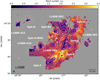 |
Fig. A.2 Similar to Fig. A.1, but with sonic Mach number as the background colour map. |
| In the text | |
|
Fig. B.1 Top panels: average NH3 (1,1) and (2,2) spectra of Oph-A core, shell-1 and shell-2 with a one-component fit. Bottom panels: same spectra, but with a two-component fit (green). The narrow (red) and broad (blue) components are also shown separately. |
| In the text | |
 |
Fig. B.2 Same as Fig. B.1, but for Oph-C. |
| In the text | |
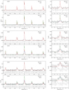 |
Fig. B.3 Same as Fig. B.1, but for Oph-D. |
| In the text | |
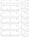 |
Fig. B.4 Same as Fig. B.1, but for Oph-E. |
| In the text | |
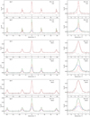 |
Fig. B.5 Same as Fig. B.1, but for Oph-F. |
| In the text | |
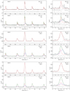 |
Fig. B.6 Same as Fig. B.1, but for Oph-B3. |
| In the text | |
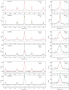 |
Fig. B.7 Same as Fig. B.1, but for Oph-H-MM1. |
| In the text | |
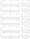 |
Fig. B.8 Same as Fig. B.1, but for L1688-d10. |
| In the text | |
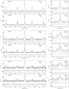 |
Fig. B.9 Same as Fig. B.1, but for L1688-d12. |
| In the text | |
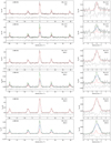 |
Fig. B.10 Same as Fig. B.1, but for L1688-SR1. |
| In the text | |
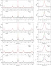 |
Fig. B.11 Same as Fig. B.1, but for L1688-SR2. |
| In the text | |
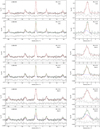 |
Fig. B.12 Same as Fig. B.1, but for L1688-SR3. |
| In the text | |
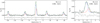 |
Fig. B.13 Alternate two-component fit to the average spectra in shell-2 of H-MM1 (see Sect. 5.5). |
| In the text | |
Current usage metrics show cumulative count of Article Views (full-text article views including HTML views, PDF and ePub downloads, according to the available data) and Abstracts Views on Vision4Press platform.
Data correspond to usage on the plateform after 2015. The current usage metrics is available 48-96 hours after online publication and is updated daily on week days.
Initial download of the metrics may take a while.