| Issue |
A&A
Volume 696, April 2025
|
|
|---|---|---|
| Article Number | A190 | |
| Number of page(s) | 10 | |
| Section | Interstellar and circumstellar matter | |
| DOI | https://doi.org/10.1051/0004-6361/202453281 | |
| Published online | 25 April 2025 | |
Asymmetric accretion through a streamer onto the pre-stellar core H-MM1
1
Korea Astronomy and Space Science Institute,
776 Daedeok-daero Yuseong-gu,
Daejeon 34055, Republic of Korea
2
Max-Planck-Institut für extraterrestrische Physik,
Giessenbachstrasse 1,
85748
Garching, Germany
3
University of Science and Technology, Korea (UST),
217 Gajeong-ro, Yuseong-gu,
Daejeon 34113, Republic of Korea
★ Corresponding author: This email address is being protected from spambots. You need JavaScript enabled to view it.
Received:
3
December
2024
Accepted:
28
February
2025
Abstract
Context. Dense cores inside molecular clouds are hubs of star formation. Cores have been thought to be isolated from their surrounding cloud. However, this idea is challenged by recent observations of streamers that show evidence of mass flow from outside the core onto the embedded protostar. Multi-component analysis using molecular line observations has also revealed the existence of subsonic material outside the traditional coherent boundary of dense cores.
Aims. In this study, we aim to probe the extended subsonic region observed around the pre-stellar core H-MM1 in the L1688 molecular cloud in Ophiuchus using multi-component kinematical analysis of very high-sensitivity NH3 data.
Methods. We used observations of NH3 (1,1) and (2,2) inversion transitions using the Green Bank Telescope (GBT). We then fitted up to two components towards the core and its surrounding molecular cloud.
Results. We detect an extended region of subsonic turbulence in addition to the ambient cloud, which shows supersonic turbulence. This extended subsonic region is approximately 12 times the size of and more than two times as massive as the previously detected subsonic material. The subsonic region is further split into two well-separated, velocity-coherent components, one of which is kinematically and spatially connected to the dense core. The two subsonic components are red- and blue-shifted with respect to the cloud component. We also detect a flow of material onto the dense core from the extended subsonic region via a streamer of length ≈0.15 pc (≈30000 au).
Conclusions. We find that the extended subsonic component kinematically associated with the dense core contains ≈27% more mass than the core. This material could be further accreted by the core. The other subsonic component contains a mass similar to that of the core mass, and could be tracing material in the early stage of core formation. The H-MM1 streamer is kinematically similar to the ones observed towards protostellar systems, but is the first instance of such an accretion feature onto a core in its pre-stellar phase. This accretion of chemically fresh material by the pre-stellar core challenges our current understanding of a core evolving with a mass that is unchanged since the time of its formation.
Key words: stars: formation / ISM: kinematics and dynamics / ISM: molecules / ISM: individual objects: H-MM1
© The Authors 2025
 Open Access article, published by EDP Sciences, under the terms of the Creative Commons Attribution License (https://creativecommons.org/licenses/by/4.0), which permits unrestricted use, distribution, and reproduction in any medium, provided the original work is properly cited.
This article is published in open access under the Subscribe to Open model. This email address is being protected from spambots. You need JavaScript enabled to view it. to support open access publication.
1 Introduction
Stars form in cold dense cores embedded in molecular clouds (Pineda et al. 2023). Cores are characterised by high densities (n ≥ 105 cm−3) and low temperatures (~10 K) (Myers 1983; Myers & Benson 1983; Caselli et al. 2002). Previous observations have also revealed a sharp transition to coherence from the turbulent ambient cloud at the boundary of dense cores (Barranco & Goodman 1998; Pineda et al. 2010).
In our current understanding of low-mass (≤ 1 M⊙) star formation, cores are treated as relatively isolated units that might collapse and form protostellar system(s) (Terebey et al. 1984; Hennebelle & Chabrier 2008; Pelkonen et al. 2021; Tsukamoto et al. 2023). In numerical simulations, cores are modelled with a mass that does not change throughout their evolution. Recent observations of streamers show asymmetric accretion of material from the disc envelope (in scales of few hundred au Hsieh et al. 2023; Flores et al. 2023; Gupta et al. 2024; Hales et al. 2024), within the core (few thousand au Alves et al. 2020), and even originating outside the natal dense core (up to 20 000 au, e.g. Pineda et al. 2020; Valdivia-Mena et al. 2022; Taniguchi et al. 2024), onto young protostellar systems. Such accretion has been observed from class II systems (Alves et al. 2020; Garufi et al. 2022) up to very young, deeply embedded class 0 stars (Le Gouellec et al. 2019; Pineda et al. 2020). These observed streamers show accretion of material by the embedded protostellar system. Kuffmeier et al. (2023) suggest that material can also be accreted from outside the dense core via streamers. This challenges the model of isolated core evolution, as accretion from outside the core will result in an increase in the core mass, which is often considered to directly relate to the mass of the star that will eventually form within it. However, such asymmetric accretion via streamers has not previously been observed towards a pre-stellar core.
NH3 inversion transitions are very useful tracers of the physical properties of structures spanning different physical scales, such as molecular clouds, filaments, and dense cores, as it can be detected in a wide range of densities. Although the critical density of NH3 is relatively low (a few times 103 cm−3 for the (1,1) and (2,2) transitions, Shirley 2015), the hyperfine structure of its inversion transitions results in the individual hyperfines remaining optically thin even at high volume densities (Caselli et al. 2017; Pineda et al. 2022). Fitting multiple hyperfines of NH3 simultaneously allows for precise constraints on the kinematical information. Moreover, a direct measurement of the gas temperature can be obtained if the NH3 (2,2) line is also reliably detected (e.g. Friesen et al. 2017).
Using multi-component analysis on NH3 observations from the Green Bank Ammonia Survey (GAS, Friesen et al. 2017), we detected gas with subsonic turbulence outside the coherent boundaries of dense cores in the molecular cloud L1688 in Ophiuchus (Choudhury et al. 2021). Our results showed the presence of extended subsonic regions outside the previously determined coherent core boundaries, and suggested that the transition to coherence might be rather gradual, in contrast to previous observations. However, due to the insufficient sensitivities of the existing data, the results in Choudhury et al. (2021) were obtained with averaged spectra towards the cores and concentric shells around each core. Therefore, we lacked the spatial resolution necessary to comment on the distribution, exact extent, and kinematics of the extended subsonic region outside the cores.
In this work, we present results from high-sensitivity observations towards the neighbourhood of the pre-stellar core H- MM1 in L1688, using NH3 (1,1) and (2,2) transitions with the Green Bank Telescope (GBT). L1688 is a molecular cloud in the Ophiuchus star-forming region, at a distance of 138.4 ± 2.6 pc (Ortiz-León et al. 2018). H-MM1 is a starless dense core (Johnstone et al. 2004; Parise et al. 2011) in the eastern part of L1688. Previous single-dish observations with NH3 (Harju et al. 2017; Choudhury et al. 2021) have shown a clear transition from supersonic to subsonic turbulence at the boundary of the core. Harju et al. (2017) reported a high degree of deuteration in the interior of H-MM1. More recently, Pineda et al. (2022) have shown the first direct observational evidence of NH3 depletion towards the centre of this core, at densities of ~105 cm−3. The sensitivity of these data allows us to reliably fit multiple components to the spectra towards the vicinity of the dense core in the native resolution. We have identified and separated the different components in the line of sight, and studied the kinematics of each component in unprecedented detail. Pineda et al. (2022) previously reported a velocity structure similar to streamers, seemingly connecting the H-MM1 core to the ambient cloud. However, they did not perform a multi-component analysis. In this work, we explore that structure with the help of a multi-component analysis. In Section 2, we describe the NH3 observations used in this work. Section 3 details the procedure used to fit the data and sort the multiple components. We present our primary results in Section 4, followed by discussions in Section 5. Our main conclusions are listed in Section 6.
2 Observations
The NH3 (1,1) and (2,2) data used in this work were taken with the GBT using the on-the-fly technique. Observations were completed in 19 sessions from November 5, 2021 to January 12, 2022 under the project GBT21B-275 (PI : S. Choudhury). We used the seven-beam K-Band Focal Plane Array (KFPA) as the front-end and the VErsatile GBT Astronomical Spectrometer (VEGAS) back-end. We used mode 20 of the VEGAS configuration, which allows eight separate spectral windows per KFPA beam. Each resultant window has a bandwidth of 23.44 MHz with 4096 spectral channels, providing a spectral resolution of 5.7 kHz (~0.07km s−1 at 23.7 GHz). To maximise the time on source, we used in-band frequency switching with a frequency throw of 4.11 MHz (≈ 50.5 km s−1) for our observations. The GBT beam at 23.7 GHz is approximately 32", with a main beam efficiency of 0.81.
The observed area was 6′ × 10′, orientated along the galactic latitude and longitude, respectively, around the pre-stellar core H-MM1. Observations were performed along the galactic longitude to minimise the overhead time. To achieve Nyquist sampling, the separation between each scan row was kept at 13′′ in galactic latitude. For all observations, the scan rate was 4′′ s−1, with data dumped every 1.6 s. We used a frequency-switching rate of 0.4 s to have four samples per integration. The pointing model was updated every 1.5-2 h, depending on weather conditions, using suitable K-band sources. The quasar 3C 286 was used for flux calibration. For data reduction, we followed the procedure described in Friesen et al. (2017), using GBTIDL1 (Marganian et al. 2006). The final data cubes were generated using all of the completed observations with GBTGRIDDER2. Figure 1 shows the resultant intensity of NH3 (1,1) and (2,2), integrated over the entire range of emission. The median noise levels obtained for both cubes were 0.04 K.
3 Analysis
3.1 Line fitting
We fitted the NH3 (1,1) and (2,2) data using the Python package pyspeckit (Ginsburg & Mirocha 2011; Ginsburg et al. 2022). We used the cold_ammonia model, which is appropriate for regions with temperatures <40 K (see Friesen et al. 2017). This model produces a synthetic model for all hyperfines of the NH3 (1,1) and (2,2) spectra with six independent parameters: kinetic and excitation temperatures (TK and Tex), NH3 column density (N(NH3)), velocity dispersion (σv), centroid velocity (vLSR), and the ortho-NH3 fraction of the total NH3 column density (fortho). Since we only have detections of the ortho-NH3 ((1,1) and (2,2) transitions), we cannot fit for fortho. Therefore, we fixed the orthoammonia fraction at 0.5 (assuming an ortho-para ratio of unity) for the fitting process. Finally, the best-fit model and the corresponding values of the six parameters (with o-NH3 fraction fixed at 0.5) were obtained using a non-linear gradient descent algorithm, MPFIT (Markwardt 2009). Fitting all of the hyperfines simultaneously allows us to obtain very precise constraints on the gas kinematics. To fit two (or three) components to the data, we added a two-component (or three-component) model as a new model in the fitter, and used this new model for the fit.
We used the Bayesian approach described in Choudhury et al. (2024) and originally presented in Sokolov et al. (2020) to fit multiple components and select the optimum number of components in the model. The best fit was selected independently for each pixel using the Bayes factor, K. Following Sokolov et al. (2020), we adopted a threshold of ln  to indicate whether model Ma was preferred over Mb.
  was defined as
 (1)
(1)
where P(Ml)s are the posterior probability densities and Zls are the likelihood integrals over the parameter space. These two parameters were calculated using the likelihood function as
 (2)
(2)
and
 (3)
(3)
where p(θ) are the prior probability densities of the parameters represented by θ. Finally, the likelihood function, L(θ), is related to χ2 as
 (4)
(4)
As initial priors for the aforementioned parameters (except ortho-NH3 fraction), we used suitable ranges to cover the values reported in Choudhury et al. (2021) for these parameters in the different components towards H-MM1 and its neighbourhood. The fitting process was iterative and automated. If the fit results indicated that the priors were inadequate for the multicomponent fits, their ranges were increased accordingly and the entire process was repeated using the new priors. The final ranges of priors thus decided for the models were uniformly distributed ranges of 5-40 K for TK, 3-15 K for Tex, 1013−1015cm−2 for  , 0.06−0.8km s−1 for σv and 2.5-5.2km s−1 for vLSR . Additionally, in order to avoid having spurious components, the minimum separation between each pair of components was required to be 0.1 km s−1 (approximately twice the spectral resolution), while the maximum separation between two components was set at 2 km s−1 (more than twice the maximum range in velocity across the observed area from single-component fit results, see Choudhury et al. 2021) to reduce the parameter space to be covered in the likelihood calculations3.
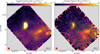 |
Fig. 1 Integrated intensity NH3 (1,1) and (2,2). The beam and scale bar are shown in the bottom left and the bottom right corners, respectively. The green contours show 15σ, 30σ, and 45σ levels for the (1,1) map and 3σ, 5σ, and 10σ levels for the (2,2) map. The root-mean-square noise levels are 0.08 K km s−1 and 0.06 K km s−1 for NH3 (1,1) and (2,2), respectively. |
3.2 Component assignment
The left panel of Fig. 2 shows the number of components fitted towards different parts of the observed region. Apart from some pixels towards the edge, we detect at least one component in the entirety of the observed region. In ≈40% of the pixels, we detect two components in the spectra. In the pixels in Fig. 2 with a single-component fit (light green), the Bayesian analysis indicates that a one-component model is a better fit than a model without any detection (noise), but a two-component model is not better than a one-component model. Similarly, for the pixels in the bluish-green region, a two-component fit is favoured over a one-component fit, but a three-component fit is not favoured over a two-component fit. As is seen in Fig. 3, there is a clear difference between the velocity dispersions of the two components. Therefore, we initially considered them as two separate components: ‘narrow’ and ‘broad’.
The panels on the right of Fig. 2 show the spectra at three representative pixels (positions marked by corresponding arrows in the left panel) in different parts of the observed region, along with the model fit. Position 1 shows a pixel with a one-component fit, and positions 2 and 3 show pixels with two- component fits. In all three panels, the total model fit is shown in green, and the residuals (model subtracted from spectrum) are shown in grey. The individual components in the two-component models (for positions 2 and 3) are shown in pink and brown, with the component with the narrower dispersion in pink and the component with the broader dispersion in brown. For both positions 2 and 3, the velocity of the broad component is similar in both positions (≈3.5 km s−1 ), while the narrow components at these two positions show clearly different velocities relative to the broad component. This suggests that the narrow component is further subdivided.
Furthermore, the centroid velocity map of the narrow component (left panel in Fig. 4) reveals that this component is not velocity-coherent. Instead, it clearly has two distinct components with median velocities of 3.23 and 4.09 km s−1. Therefore, we further separated the narrow component into two components: narrow-blue and narrow-red, according to their velocity shift from the broad component (Fig. 4).
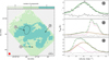 |
Fig. 2 Left: number of components detected towards the observed region. These components are later grouped into three separate components according to their kinematical properties (see Section 3.2). The solid black contour shows the boundary of the coherent region obtained with a single-component fit. The beam and scale bar are shown in the bottom left and the bottom right corners, respectively. Right: examples of NH3 (1,1) spectra with the obtained fit, at the positions indicated in the left panel. Only a small range in velocity is shown here to clearly highlight the individual components. In each panel, the fitted model is shown in green, while the residuals are shown in grey. Positions 2 and 3 show two- component fits. The individual components are shown in brown and pink, with the component with the larger linewidth shown in brown. Note the multiple, closely spaced hyperfines in the velocity range shown here. The strongest two of these hyperfines can be individually seen in the narrow component (pink) at position 2. For all other cases shown here, these hyperfines are blended together due to the broad linewidth of the spectra. |
4 Results
4.1 Kinematics of the identified velocity components
We identified three separate velocity-coherent components with our multi-component analysis. Two of the components (narrowblue and narrow-red) show subsonic turbulence in the entire region where they are detected, while the other component is turbulent. In our discussion, ‘turbulence’ refers to the nonthermal velocity dispersion, σv,NT, calculated by removing the thermal dispersion for the observed molecule (σT) from the total observed velocity dispersion (σv):
 (5)
(5)
Here, σchan is the spectral response, which is negligible in this observation (=0.036 km s−1, Choudhury et al. 2021). The thermal component of NH3 velocity dispersion is
 (6)
(6)
where kB is the Boltzmann’s constant and TK is the kinetic temperature in the region, with  amu being the mass of the ammonia molecule. Then, the sonic Mach number (MS) is defined as the ratio of the non-thermal velocity dispersion to the sound speed in the medium:
 (7)
(7)
where cs is the one-dimensional sound speed in the gas, given by:
 (8)
(8)
with µgas being the average molecular mass (taken to be 2.37 amu, Kauffmann et al. 2008).
The velocity dispersion and the centroid velocities of the components detected in this work are shown in Figs. 3 and 4. The velocity of the turbulent (broad) component ranges from 3.3 km s−1 to 3.9 km s−1, with a clearly visible large-scale gradient from north-east to south-west. However, it shows no sharp changes in velocity, suggesting that it is a single, continuous component. This fact, combined with the presence of supersonic turbulence (MS = 1.8, corresponding to a median velocity dispersion of  km s−1) in the component, suggests that it is . tracing the ambient cloud towards the region. It should be noted that the errors associated with the median values mentioned here (and in the subsequent section) refer to the difference of the 16th and the 84th percentiles of the population from the median value.
The two subsonic components (narrow-red and narrow-blue) are red- and blue-shifted, respectively, relative to the cloud component. The narrow-red component is spatially and kinematically consistent with the core material. Therefore, we conclude that this component is tracing an extended core region, an area larger than that of the previously identified coherent core (shown with black contours in the figures). The velocity of this component is nearly constant, with a median of 4.09 km s−1, and the difference between the 16th and the 84th percentiles is less than 0.15 km s−1. The turbulence in this component is highly subsonic, with a velocity dispersion of  . The narrow-blue component shows a velocity dispersion similar to that of the narrow-red one, with a slightly larger spread. The median dispersion of this component is
  .However, it lies at a clearly distinct velocity of 3.23 km s−1. There is a small observable gradient in velocity from west to east. This is also reflected in the difference between the 16th and the 84th percentiles, which is 0.26 km s−1. We note that there is a small (<0.5 km s−1 ) difference in the velocity of this component in the north-south and east-west directions, which follows the larger-scale velocity fluctuations seen in the cloud component (right panel in Fig. 4). There is no clear gradient in the velocity of the narrow-blue component relative to the cloud.
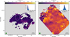 |
Fig. 3 Velocity dispersions of the narrow component (left) and the broad component (right). The probability distribution function of the velocity dispersion of the respective component is shown in the inset in the top right corner of each figure. The vertical red lines in the insets show the median dispersion of each component. The turbulence in the narrow component is consistently subsonic throughout, whereas the broad component is always supersonic (the velocity dispersion for sonic turbulence at these temperatures is ≈0.2km s−1). The solid white contour shows the boundary of the coherent core from single-component fits. The beam and scale bar are shown in the bottom left and bottom right corners, respectively. |
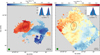 |
Fig. 4 Velocities of the narrow (subsonic turbulence) component (left) and the broad (supersonic turbulence) component (right). The probability distribution function of the velocity of each component is shown in the insets in the top right corners of the figures. It can be seen that the narrow component is clearly further subdivided into two additional velocity components with median velocities of 3.23 km s−1 and 4.09 km s−1, while the broad component lies at a median velocity of 3.6 km s−1. (The median velocities of the different components are shown by the vertical red lines in the insets.) The solid black contour shows the boundary of the coherent core from single-component fits. The beam and scale bar are shown in the bottom left and the bottom right corners, respectively. |
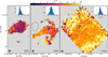 |
Fig. 5 Kinetic temperature of the narrow-red (left), narrow-blue (middle), and broad (right) components. The common colour scale is shown at the top. The inset in the top right corner of each figure shows the probability distribution function of the temperature of the respective component. The vertical red lines in the insets show the median of that distribution. The narrow component is considerably cooler than the broad component throughout, especially in the vicinity of the coherent dense core, shown by the black contour. The blue-shifted part of the narrow component shows a slightly warmer temperature than the red-shifted counterpart. The solid black contour shows the boundary of the coherent core from singlecomponent fits. The beam and scale bar are shown in the bottom left and the bottom right corners, respectively. |
4.2 Temperatures of the components
Figure 5 shows the kinetic temperature of the three components, derived from fitting NH3 (1,1) and (2,2) lines. We can clearly see a systematic difference in the temperature of the broad component compared to the narrow components. The broad component is at a median temperature of  , whereas the narrow-red and narrow-blue components are at
  and
and  , respectively. The difference between the temperature distribution of each component can also be seen from their probability distribution, shown in insets in Fig. 5.
As was expected, the narrow-red component is at low temperatures characteristic of core material. Similarly, the broad component shows temperatures of around 20 K, which is typical for the warm ambient molecular cloud. On the other hand, the narrow-blue material is at a temperature of 15 K, which is warmer than typical core material, but cooler than ambient cloud. The east part of this component is at a slightly higher temperature compared to the west, with a difference of approximately 2 K.
5 Discussion
5.1 Extended subsonic region associated with the dense core
Figure 6 shows the sonic Mach number in the region using a single-component fit to the data. The region with MS ≤ 1 is shown in solid black contours. As previous studies typically employed a single-component analysis, this contour represents the boundary of the coherent core, determined previously. However, as was mentioned above, with the high sensitivity of our data, and using a multi-component analysis, we are able to detect a much larger region of subsonic turbulence, divided into two velocity-coherent regions: narrow-red and narrow-blue. The combined subsonic boundary of these two regions is shown with dashed black contours in Figure 6. With a two-component analysis, we recover a subsonic area that is approximately 12 times larger than the area of the coherent core from previous observations. This previously undetected and substantially larger region of subsonic turbulence indicates that there is much more material available for accretion by the core than previous estimates suggested.
As NH3 is a poor indicator of densities, we cannot obtain an accurate measurement of the mass contained in these different regions. However, Schmiedeke et al. (2021) showed a correlation between the observed NH3 flux and that of dust continuum, yielding a direct conversion between NH3 flux and mass. Therefore, we can use the total NH3 flux in the respective components in each region as a proxy for the enclosed mass. We computed the total flux in NH3 (1,1) inside the coherent core boundary (solid black contour) in Fig. 6 using a single-component fit model. This flux can be considered as indicative of the mass of the previously estimated coherent region, as the previous studies used a single-component fit in their analysis. Similarly, we can estimate the mass of the extended subsonic region we detect in this work (dashed black contours in Figure 6) from the total NH3 (1,1) flux in the narrow component (left panel of Fig. 3). Comparing the two, we find that the mass enclosed in the extended subsonic region is 113% more than that of the previously estimated coherent region. This means that a significantly large amount of subsonic material was previously undetected due to insufficient sensitivities. This subsonic material could be further accreted by the core (for narrow-red component), or form another core (narrow-blue component).
The narrow-red component, which is kinematically and spatially connected to the dense core, contains additional mass outside the previously calculated core boundary (left panel of Figure 4). Comparing the total NH3 (1,1) flux in the narrow-red component inside the core boundary and outside of it, we find that the amount of additional mass is ~27% of the core mass. This implies that the mass of the core can increase by this amount during its evolution by accreting the subsonic material that is physically connected to the core. Similarly, by calculating the total flux in NH3 (1,1) in the narrow-blue component, we find that this component contains a mass similar to that of the core (≈90% of the core mass). This component is kinematically similar to core material, but its temperature is intermediate between that of typical dense cores and ambient cloud. This region could be material in the process of forming a core, with a mass similar to that of H-MM1 (see Section 5.2).
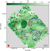 |
Fig. 6 Sonic Mach number, calculated using a single-component fit. The solid black contour shows the boundary of the subsonic region in this map, which is similar to the previously determined boundary of the coherent dense core. The dashed black contour shows the boundary of the extended subsonic region that can only be detected using multicomponent analysis as described in this work. The dotted red and dotted blue contours show the extents of the narrow-red and narrow-blue components, respectively. The beam and scale bar are shown in the bottom left and the bottom right corners, respectively. |
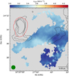 |
Fig. 7 Velocity map of the narrow-blue component, with N(H2 ) obtained from Herschel observations overlaid as dashed black contours. The contour levels indicate N(H2) = 1.2 × 1022,1.3 × 1022,1.5 × 1022, 1.8 × 1022 cm−2. The red contour shows the boundary of the coherent core from single-component fits. The beam and scale bar are shown in the bottom left and the bottom right corners, respectively. |
5.2 Origin of the narrow-blue component
As was discussed in previous sections, in this work we detect three separate velocity-coherent components towards the neighbourhood of H-MM1. Similar to our previous results in Choudhury et al. (2021), two of those components correspond to material associated with the dense core and the ambient cloud. However, here we detect a third component in the line of sight, which does not appear to represent either the known core or the cloud. This component (narrow-blue) has a velocity dispersion very similar to that of the core, albeit with a slightly larger spread of ≈0.1km s−1. However, it has a completely different velocity from the core, and lies on the opposite side of the cloud in the velocity plane. These features indicate that, although similarly subsonic as the core, the narrow-blue component is tracing a completely separate region.
This component has a kinetic temperature that is intermediate between characteristic temperatures of typical dense cores and large-scale molecular clouds, which suggests that this region is intermediate between core and cloud. Figure 7 shows this component overlaid with contours of N(H2) taken from the Herschel Gould Belt Survey (Arzoumanian et al. 2019; Ladjelate et al. 2020). It can be seen that there is a small local peak in the column density around the centre of the region traced by this component. It can be noted that Ladjelate et al. (2020) identify a bound starless core at this location.
Therefore, the narrow-blue component is tracing gas that has dissipated its turbulence and that is in the process of cooling down from the molecular cloud temperatures. Moreover, it shows a local peak in the column density inside the region. These physical and kinetic properties indicate that this component might be tracing material in the early stages of core formation, similar to ‘Phase II’ cores, or coherent, bound cores showing low turbulence, as categorised by Offner et al. (2022) using a magnetohydrodynamic simulation of a star-forming cloud.
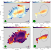 |
Fig. 8 Centroid velocity (top) and velocity dispersion (bottom) of the narrow-red component. The colour scales used here are different from the ones used in the previous figures, with a smaller range chosen to highlight the kinematic features. The panels on the right show the velocity and dispersion of the elongated red-shifted feature. The solid black or solid white contour shows the boundary of the coherent core from singlecomponent fits. The beam and scale bar are shown in the bottom left and the bottom right corners, respectively. |
5.3 Possible infall into the core
Figure 8 shows a zoom-in view of the velocity and velocity dispersion of the narrow-red component. The dynamic ranges shown in this figure are smaller than the ones in the previous figures in order to clearly show an elongated kinematic feature towards the core. This feature was also observed in high-resolution Very Large Array (VLA) observations with NH3 towards H-MM1, by Pineda et al. (2022).
This elongated region is slightly red-shifted, at ≈4.18 km s−1, compared to the rest of the core material at ≈4.09km s−1, and extends from outside the core boundary towards the east, with a total length of ≈0.15 pc, or ≈30 000 au. The region where this feature interacts with the core material shows a slightly higher velocity dispersion, with a peak of 0.17 km s−1, compared to the rest of the core, where the velocity dispersion is 0.12 km s−1. Observations of streamers also show a smooth velocity gradient towards the centre, with an increase in the velocity gradient where the streamer meets the protostellar system (Pineda et al. 2020; Thieme et al. 2022; Valdivia-Mena et al. 2022; Hsieh et al. 2023; Flores et al. 2023). Therefore, the feature observed towards H-MM1 is kinematically similar to streamers. However, it is to be noted that the velocity gradient and the increase in velocity dispersion towards the centre are almost an order of magnitude higher in the case of streamers (≈ 1 km s−1 and ≈0.5 km s−1, respectively). This is expected, as the streamers are observed with a much higher resolution, probing very close to the central star, and as there is a protostar at the centre of the infall.
However, in the case of H-MM1, there are no known protostars embedded inside the core. Therefore, it is a much younger system than the ones of the previously observed streamers. Furthermore, the larger GBT beam likely causes smoothening of the small-scale kinematical variations. Therefore, the velocity gradient and the increase in velocity dispersion observed in this feature are quantitatively less than the ones observed in streamers.
This elongated red-shifted feature appears to be tracing mass accretion by the core itself from the extended subsonic region outside its boundary. This could be the first evidence of large- scale asymmetric accretion by a pre-stellar core, in that the accreting material is penetrating the core from one specific direction, similar to the streamers observed towards protostellar discs.
The relatively large GBT beam likely smoothens out the velocity gradient in this structure, which makes further kinematic analysis difficult, especially since the velocity difference between different parts of the observed region is already quite small. Interferometric spectral line observations are required to trace this feature to its largest extent, and compare its kinematics with infall models, similar to streamers. Observations with carbon-chain molecules such as CCS, HC3N, and HC5N, which trace chemically young regions (Suzuki et al. 1992), and tracers of more chemically evolved gas like N2H+ and DCN, will provide insights into the origin of the streamer material (Pineda et al. 2020; Murillo et al. 2022; Hsieh et al. 2023; Taniguchi et al. 2024). Chemically young regions are characterised by large abundances of atomic carbon in the gas phase (as carbon has not yet been mainly locked in CO), which is needed to produce carbon-chain molecules efficiently.
6 Conclusions
We used high-sensitivity GBT observations of the pre-stellar core H-MM1 and its neighbourhood in the L1688 molecular cloud in Ophiuchus to study the multi-component structure of the gas towards the core and its immediate surroundings. Our results can be summarised as follows:
Using a multi-component fit to the spectra in the line of sight, we separated the core and cloud in the line of sight, thereby allowing us to analyse the core material in more physical detail;
We detect an extended subsonic region significantly larger than the previously observed coherent core: approximately 12 times larger in area, and approximately two times more massive;
We find that the subsonic region is not continuous, but rather divided into two distinct velocity-coherent regions. One of these components, narrow-red, is spatially and kinematically linked to the dense core material. Therefore, we conclude that this component traces the core and the extended subsonic material connected to the core;
Additionally, we detect a subsonic component, narrow-blue, which traces a more extended, lower-density region, with a kinetic temperature that is intermediate between that of typical dense cores and that of the ambient molecular cloud. There is a local peak observed in N(H2) at the heart of this region, where Ladjelate et al. (2020) report a starless bound core. Therefore, this extended component could be tracing material from a core in the early stages of formation;
We find a narrow velocity structure towards the centre of the core from the extended subsonic region, with a smooth velocity gradient. We also observe a local increase in the velocity dispersion where this structure meets the inner part of the core. Therefore, we conclude that this feature likely shows the flow of material from the ambient cloud to the pre-stellar core H-MM1 via a streamer.
The results from this work show the importance of a multicomponent analysis and the usefulness of high-sensitivity observations. With our analysis, we have been able to separate multiple components in the line of sight and recover a much larger subsonic region than was previously observed. We have also found a previously undetected subsonic component likely associated with an early core. Moreover, we detect evidence of flow of gas from the ambient cloud to a pre-stellar core. Such accretion of chemically fresh gas onto dense cores during its evolution implies the need for a significant update to current physical and chemical models of core evolution.
Acknowledgements
C.W.L. acknowledges support from the Basic Science Research Program through the NRF funded by the Ministry of Education, Science and Technology (NRF-2019R1A2C1010851) and by the Korea Astronomy and Space Science Institute grant funded by the Korean government (MSIT; project No. 2024-1-841-00).
References
- Alves, F. O., Cleeves, L. I., Girart, J. M., et al. 2020, ApJ, 904, L6 [Google Scholar]
- Arzoumanian, D., André, P., Könyves, V., et al. 2019, A&A, 621, A42 [Google Scholar]
- Barranco, J. A., & Goodman, A. A. 1998, ApJ, 504, 207 [Google Scholar]
- Caselli, P., Benson, P. J., Myers, P. C., & Tafalla, M. 2002, ApJ, 572, 238 [Google Scholar]
- Caselli, P., Bizzocchi, L., Keto, E., et al. 2017, A&A, 603, L1 [Google Scholar]
- Choudhury, S., Pineda, J. E., Caselli, P., et al. 2021, A&A, 648, A114 [Google Scholar]
- Choudhury, S., Pineda, J. E., Caselli, P., et al. 2024, A&A, 683, A77 [Google Scholar]
- Flores, C., Ohashi, N., Tobin, J. J., et al. 2023, ApJ, 958, 98 [Google Scholar]
- Friesen, R. K., Pineda, J. E., co-PIs, et al. 2017, ApJ, 843, 63 [Google Scholar]
- Garufi, A., Podio, L., Codella, C., et al. 2022, A&A, 658, A104 [Google Scholar]
- Ginsburg, A., & Mirocha, J. 2011, PySpecKit: Python Spectroscopic Toolkit, Astrophysics Source Code Library [record ascl:1109.001] [Google Scholar]
- Ginsburg, A., Sokolov, V., de Val-Borro, M., et al. 2022, AJ, 163, 291 [Google Scholar]
- Gupta, A., Miotello, A., Williams, J. P., et al. 2024, A&A, 683, A133 [Google Scholar]
- Hales, A. S., Gupta, A., Ruiz-Rodriguez, D., et al. 2024, ApJ, 966, 96 [Google Scholar]
- Harju, J., Daniel, F., Sipilä, O., et al. 2017, A&A, 600, A61 [Google Scholar]
- Hennebelle, P., & Chabrier, G. 2008, ApJ, 684, 395 [Google Scholar]
- Hsieh, T. H., Segura-Cox, D. M., Pineda, J. E., et al. 2023, A&A, 669, A137 [Google Scholar]
- Johnstone, D., Di Francesco, J., & Kirk, H. 2004, ApJ, 611, L45 [Google Scholar]
- Kauffmann, J., Bertoldi, F., Bourke, T. L., Evans, N. J. I., & Lee, C. W. 2008, A&A, 487, 993 [Google Scholar]
- Kuffmeier, M., Jensen, S. S., & Haugbølle, T. 2023, Eur. Phys. J. Plus, 138, 272 [Google Scholar]
- Ladjelate, B., André, P., Konyves, V., et al. 2020, A&A, 638, A74 [Google Scholar]
- Le Gouellec, V. J. M., Hull, C. L. H., Maury, A. J., et al. 2019, ApJ, 885, 106 [Google Scholar]
- Marganian, P., Garwood, R. W., Braatz, J. A., et al. 2006, Astronomical Data Analysis Software and Systems XV, eds. C. Gabriel, C. Arviset, D. Ponz, & S. Enrique, Astron. Soc. Pacific Conf. Ser., 351, 512 [Google Scholar]
- Markwardt, C. B. 2009, in Astronomical Data Analysis Software and Systems XVIII, eds. D. A. Bohlender, D. Durand, & P. Dowler, Astronomical Society of the Pacific Conference Series, 411, 251 [Google Scholar]
- Murillo, N. M., van Dishoeck, E. F., Hacar, A., Harsono, D., & Jørgensen, J. K. 2022, A&A, 658, A53 [Google Scholar]
- Myers, P. C. 1983, ApJ, 270, 105 [Google Scholar]
- Myers, P. C., & Benson, P. J. 1983, ApJ, 266, 309 [Google Scholar]
- Offner, S. S. R., Taylor, J., Markey, C., et al. 2022, MNRAS, 517, 885 [Google Scholar]
- Ortiz-León, G. N., Loinard, L., Dzib, S. A., et al. 2018, ApJ, 869, L33 [Google Scholar]
- Parise, B., Belloche, A., Du, F., Güsten, R., & Menten, K. M. 2011, A&A, 526, A31 [Google Scholar]
- Pelkonen, V. M., Padoan, P., Haugbølle, T., & Nordlund, Å. 2021, MNRAS, 504, 1219 [Google Scholar]
- Pineda, J. E., Goodman, A. A., Arce, H. G., et al. 2010, ApJ, 712, L116 [Google Scholar]
- Pineda, J. E., Segura-Cox, D., Caselli, P., et al. 2020, Nat. Astron., 4, 1158 [Google Scholar]
- Pineda, J. E., Harju, J., Caselli, P., et al. 2022, AJ, 163, 294 [Google Scholar]
- Pineda, J. E., Arzoumanian, D., Andre, P., et al. 2023, in Protostars and Planets VII, eds. S. Inutsuka, Y. Aikawa, T. Muto, K. Tomida, & M. Tamura, Astronomical Society of the Pacific Conference Series, 534, 233 [Google Scholar]
- Schmiedeke, A., Pineda, J. E., Caselli, P., et al. 2021, ApJ, 909, 60 [Google Scholar]
- Shirley, Y. L. 2015, PASP, 127, 299 [Google Scholar]
- Sokolov, V., Pineda, J. E., Buchner, J., & Caselli, P. 2020, ApJ, 892, L32 [Google Scholar]
- Suzuki, H., Yamamoto, S., Ohishi, M., et al. 1992, ApJ, 392, 551 [Google Scholar]
- Taniguchi, K., Pineda, J. E., Caselli, P., et al. 2024, ApJ, 965, 162 [Google Scholar]
- Terebey, S., Shu, F. H., & Cassen, P. 1984, ApJ, 286, 529 [Google Scholar]
- Thieme, T. J., Lai, S.-P., Lin, S.-J., et al. 2022, ApJ, 925, 32 [Google Scholar]
- Tsukamoto, Y., Maury, A., Commercon, B., et al. 2023, in Protostars and Planets VII, eds. S. Inutsuka, Y. Aikawa, T. Muto, K. Tomida, & M. Tamura, Astronomical Society of the Pacific Conference Series, 534, 317 [Google Scholar]
- Valdivia-Mena, M. T., Pineda, J. E., Segura-Cox, D. M., et al. 2022, A&A, 667, A12 [Google Scholar]
The scripts and data files used in the analysis presented in this paper, including the scripts to make the parameter maps, can be accessed at https://github.com/SpandanCh/H-MM1_extended_subsonic
All Figures
|
Fig. 1 Integrated intensity NH3 (1,1) and (2,2). The beam and scale bar are shown in the bottom left and the bottom right corners, respectively. The green contours show 15σ, 30σ, and 45σ levels for the (1,1) map and 3σ, 5σ, and 10σ levels for the (2,2) map. The root-mean-square noise levels are 0.08 K km s−1 and 0.06 K km s−1 for NH3 (1,1) and (2,2), respectively. |
| In the text | |
|
Fig. 2 Left: number of components detected towards the observed region. These components are later grouped into three separate components according to their kinematical properties (see Section 3.2). The solid black contour shows the boundary of the coherent region obtained with a single-component fit. The beam and scale bar are shown in the bottom left and the bottom right corners, respectively. Right: examples of NH3 (1,1) spectra with the obtained fit, at the positions indicated in the left panel. Only a small range in velocity is shown here to clearly highlight the individual components. In each panel, the fitted model is shown in green, while the residuals are shown in grey. Positions 2 and 3 show two- component fits. The individual components are shown in brown and pink, with the component with the larger linewidth shown in brown. Note the multiple, closely spaced hyperfines in the velocity range shown here. The strongest two of these hyperfines can be individually seen in the narrow component (pink) at position 2. For all other cases shown here, these hyperfines are blended together due to the broad linewidth of the spectra. |
| In the text | |
|
Fig. 3 Velocity dispersions of the narrow component (left) and the broad component (right). The probability distribution function of the velocity dispersion of the respective component is shown in the inset in the top right corner of each figure. The vertical red lines in the insets show the median dispersion of each component. The turbulence in the narrow component is consistently subsonic throughout, whereas the broad component is always supersonic (the velocity dispersion for sonic turbulence at these temperatures is ≈0.2km s−1). The solid white contour shows the boundary of the coherent core from single-component fits. The beam and scale bar are shown in the bottom left and bottom right corners, respectively. |
| In the text | |
|
Fig. 4 Velocities of the narrow (subsonic turbulence) component (left) and the broad (supersonic turbulence) component (right). The probability distribution function of the velocity of each component is shown in the insets in the top right corners of the figures. It can be seen that the narrow component is clearly further subdivided into two additional velocity components with median velocities of 3.23 km s−1 and 4.09 km s−1, while the broad component lies at a median velocity of 3.6 km s−1. (The median velocities of the different components are shown by the vertical red lines in the insets.) The solid black contour shows the boundary of the coherent core from single-component fits. The beam and scale bar are shown in the bottom left and the bottom right corners, respectively. |
| In the text | |
|
Fig. 5 Kinetic temperature of the narrow-red (left), narrow-blue (middle), and broad (right) components. The common colour scale is shown at the top. The inset in the top right corner of each figure shows the probability distribution function of the temperature of the respective component. The vertical red lines in the insets show the median of that distribution. The narrow component is considerably cooler than the broad component throughout, especially in the vicinity of the coherent dense core, shown by the black contour. The blue-shifted part of the narrow component shows a slightly warmer temperature than the red-shifted counterpart. The solid black contour shows the boundary of the coherent core from singlecomponent fits. The beam and scale bar are shown in the bottom left and the bottom right corners, respectively. |
| In the text | |
|
Fig. 6 Sonic Mach number, calculated using a single-component fit. The solid black contour shows the boundary of the subsonic region in this map, which is similar to the previously determined boundary of the coherent dense core. The dashed black contour shows the boundary of the extended subsonic region that can only be detected using multicomponent analysis as described in this work. The dotted red and dotted blue contours show the extents of the narrow-red and narrow-blue components, respectively. The beam and scale bar are shown in the bottom left and the bottom right corners, respectively. |
| In the text | |
|
Fig. 7 Velocity map of the narrow-blue component, with N(H2 ) obtained from Herschel observations overlaid as dashed black contours. The contour levels indicate N(H2) = 1.2 × 1022,1.3 × 1022,1.5 × 1022, 1.8 × 1022 cm−2. The red contour shows the boundary of the coherent core from single-component fits. The beam and scale bar are shown in the bottom left and the bottom right corners, respectively. |
| In the text | |
|
Fig. 8 Centroid velocity (top) and velocity dispersion (bottom) of the narrow-red component. The colour scales used here are different from the ones used in the previous figures, with a smaller range chosen to highlight the kinematic features. The panels on the right show the velocity and dispersion of the elongated red-shifted feature. The solid black or solid white contour shows the boundary of the coherent core from singlecomponent fits. The beam and scale bar are shown in the bottom left and the bottom right corners, respectively. |
| In the text | |
Current usage metrics show cumulative count of Article Views (full-text article views including HTML views, PDF and ePub downloads, according to the available data) and Abstracts Views on Vision4Press platform.
Data correspond to usage on the plateform after 2015. The current usage metrics is available 48-96 hours after online publication and is updated daily on week days.
Initial download of the metrics may take a while.