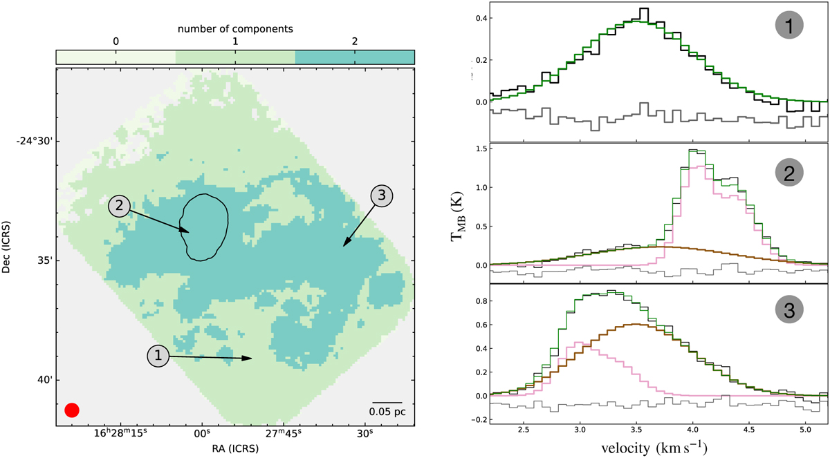
Fig. 2
Download original image
Left: number of components detected towards the observed region. These components are later grouped into three separate components according to their kinematical properties (see Section 3.2). The solid black contour shows the boundary of the coherent region obtained with a single-component fit. The beam and scale bar are shown in the bottom left and the bottom right corners, respectively. Right: examples of NH3 (1,1) spectra with the obtained fit, at the positions indicated in the left panel. Only a small range in velocity is shown here to clearly highlight the individual components. In each panel, the fitted model is shown in green, while the residuals are shown in grey. Positions 2 and 3 show two- component fits. The individual components are shown in brown and pink, with the component with the larger linewidth shown in brown. Note the multiple, closely spaced hyperfines in the velocity range shown here. The strongest two of these hyperfines can be individually seen in the narrow component (pink) at position 2. For all other cases shown here, these hyperfines are blended together due to the broad linewidth of the spectra.
Current usage metrics show cumulative count of Article Views (full-text article views including HTML views, PDF and ePub downloads, according to the available data) and Abstracts Views on Vision4Press platform.
Data correspond to usage on the plateform after 2015. The current usage metrics is available 48-96 hours after online publication and is updated daily on week days.
Initial download of the metrics may take a while.