| Issue |
A&A
Volume 699, July 2025
|
|
|---|---|---|
| Article Number | A88 | |
| Number of page(s) | 18 | |
| Section | Cosmology (including clusters of galaxies) | |
| DOI | https://doi.org/10.1051/0004-6361/202555417 | |
| Published online | 02 July 2025 | |
CHEX-MATE: Exploring the kinematical properties of Planck galaxy clusters⋆
1
Dipartimento di Fisica G. Occhialini, Università degli Studi di Milano Bicocca, Piazza della Scienza 3, I-20126 Milano, Italy
2
Instituto de Astrofísica de Canarias, C/ Vía Láctea s/n, E-38205 La Laguna, Tenerife, Spain
3
Universidad de La Laguna, Departamento de Astrofísica, E-38206 La Laguna, Tenerife, Spain
4
INAF – Osservatorio di Astrofisica e Scienza dello Spazio di Bologna, Via Piero Gobetti 93/3, I-40129 Bologna, Italy
5
INFN, Sezione di Bologna, Viale Berti Pichat 6/2, I-40127 Bologna, Italy
6
Dipartimento di Fisica ‘E. Pancini’, Università degli Studi di Napoli Federico II, Via Cinthia, 21, I-80126 Napoli, Italy
7
Université Côte d’Azur, Observatoire de la Côte d’Azur, CNRS, Laboratoire Lagrange, Bd de l’Observatoire, CS 34229, 06304 Nice Cedex 4, France
8
Université Paris-Saclay, Université Paris Cité, CEA, CNRS, AIM, 91191 Gif-sur-Yvette, France
9
Michigan State University, Physics and Astronomy Department, 567 Wilson Road, East Lansing, Michigan 48824, USA
10
INAF, Istituto di Astrofisica Spaziale e Fisica Cosmica di Milano, Via A. Corti 12, 20133 Milano, Italy
11
Laboratoire d’Astrophysique de Marseille, Aix-Marseille Univ., CNRS, CNES, 13013 Marseille, France
12
Institut d’Astrophysique de Paris, UMR7095 CNRS & Sorbonne Université, 98bis Bd Arago, 75014 Paris, France
13
Instituto de Astronomía y Ciencias Planetarias, Universidad de Atacama, Copayapu 485, Copiapó, Chile
14
Millennium Nucleus for Galaxies (MINGAL), Valparaíso, Chile
15
Jodrell Bank Centre for Astrophysics, Department of Physics and Astronomy, University of Manchester, Manchester M13 9PL, UK
16
Center for Astrophysics | Harvard \AMP Smithsonian, 60 Garden Street, Cambridge, MA 02138, USA
17
HH Wills Physics Laboratory, University of Bristol, Tyndall Ave, Bristol BS8 1TL, UK
18
IRAP, CNRS, Université de Toulouse, CNES, Toulouse, France
19
Osservatorio Astronomico di Trieste, Via Tiepolo 11, I-34131 Trieste, Italy
20
IFPU, Institute for Fundamental Physics of the Universe, Via Beirut 2, 34014 Trieste, Italy
21
Department of Physics, University of Michigan, Ann Arbor, MI 48109, USA
22
INAF – Osservatorio Astronomico di Padova, Vicolo Osservatorio 5, I-35122 Padova, Italy
23
California Institute of Technology, Pasadena, CA 91125, USA
⋆⋆ Corresponding author.
Received:
7
May
2025
Accepted:
23
May
2025
Abstract
We analysed the kinematical properties of the CHEX-MATE galaxy cluster sample. Our study is based on the radial velocities retrieved from the SDSS DR18, DESI, and NED spectroscopic databases and new data obtained with the 10.4 m GTC and ESO-NTT telescopes. We derived cluster mass profiles for 75 clusters using the MG-MAMPOSST procedure, which recovers the gravitational potential and the anisotropy profiles from line-of-sight velocities and projected positions of galaxy members. The standard Navarro–Frenk–White (NFW) model and the Burkert model, with flatter cores than the NFW, both adequately fit the kinematic data, with only a marginal statistical preference for one model over the other. An estimation of the mass bias (1−B1) = M500SZ/M500M was performed via a comparison with Sunyaev-Zel’dovich–X-ray-calibrated mass estimates, resulting in a value of 0.54 ± 0.11 when four evidently disturbed clusters are removed from the sample. We assessed the dynamical state of the clusters by inferring the Anderson-Darling coefficient (A2) and the fraction of galaxies in substructures (fsub). Except for a few cases, we find relatively low values for A2, which suggests that CHEX-MATE clusters are not too far from relaxation. Moreover, no significant trends emerge between A2 and fsub, nor between the log-masses estimated by MG-MAMPOSST and those based on the Sunyaev–Zel’dovich effect calibrated through X-rays measurements. We studied the concentration–mass relation for the sample; despite the large scatter, we observe signs of an increasing trend for high-mass clusters, in agreement with recent theoretical expectations. Finally, our analysis of the radial anisotropy profiles of member galaxies – stacked in five bins of mass and redshift – reveals that orbits tend to be isotropic at the centre and more radial towards the edge, as found in previous studies. A slight trend of increasing radial orbits at r200 is observed in clusters with larger velocity dispersions.
Key words: galaxies: clusters: general / galaxies: kinematics and dynamics
Based in part on observations collected at the European Southern Observatory under ESO programmes 0110.A-4192 and 0111.1-0186.
© The Authors 2025
 Open Access article, published by EDP Sciences, under the terms of the Creative Commons Attribution License (https://creativecommons.org/licenses/by/4.0), which permits unrestricted use, distribution, and reproduction in any medium, provided the original work is properly cited.
This article is published in open access under the Subscribe to Open model. This email address is being protected from spambots. You need JavaScript enabled to view it. to support open access publication.
1. Introduction
Galaxy clusters are the most massive virialised structures in the Universe and, as such, are excellent natural laboratories to study the formation, structure assembly, and evolution of mass halos and sub-halos across cosmic time. The combination of optical data, X-ray observations, and the signal from the Sunyaev–Zel’dovich (SZ) effect (Sunyaev & Zeldovich 1972) is ideal for studying galaxy clusters. A multi-wavelength analysis allows us to acquire a complete picture of the physics behind different components – dark matter (Zwicky 1933), gas (Cavaliere & Fusco-Femiano 1981), and galaxies (e.g. Abell 1958) – and see how they interact to configure these massive objects.
In this work we studied dynamical cluster mass profiles, the presence of substructures, and velocity anisotropies by analysing the projected-phase-space (PPS) distribution of member galaxies (e.g. Carlberg et al. 1997) under the assumption of dynamical equilibrium. As galaxies enter into clusters through hierarchical accretion, their orbits contain important information on the processes that lead to cluster mass assembly and internal dynamical relaxation (e.g. Biviano & Katgert 2004). Moreover, knowledge of the orbits of cluster galaxies is crucial to understanding environmental effects that differentiate galaxy evolution in clusters from those in the field (Lotz et al. 2019; Tonnesen 2019).
Our studies were carried out using the MG-MAMPOSST (Modelling Anisotropy and Mass Profile of Spherical Observed Systems) code from Pizzuti et al. (2023). This technique allows us to reconstruct cluster mass profiles and velocity anisotropy profiles for several parametrisations of the total gravitational potential, in general relativity and in general dark energy or modified gravity frameworks. In other words, MG-MAMPOSST jointly obtains the best-fit parameters for the cluster mass distribution and for the velocity anisotropy profile of cluster members (Munari et al. 2014; Zarattini et al. 2021); this analysis allows us to retrieve information about the orbits of galaxies by distinguishing, statistically, between populations with radial and circular configurations.
We developed our analysis using the Cluster HEritage project with XMM-Newton – Mass Assembly and Thermodynamics at the Endpoint of structure formation (CHEX-MATE) cluster sample (CHEX-MATE Collaboration 2021). This project is based on the three-mega-second Multi-Year Heritage Programme, whose goal is to obtain X-ray observations of a minimally biased, signal-to-noise-limited (S/N > 6.5) sample of 118 galaxy clusters detected by Planck through the SZ effect. The CHEX-MATE census contains two subsamples: Tier 1 (T1), which includes a census of the population at the most recent time (0.05 < z < 0.2), and Tier 2 (T2), the most massive objects to have formed at z < 0.6 (see Fig. 1 in CHEX-MATE Collaboration 2021). Therefore, the CHEX-MATE clusters offer us the opportunity to study the kinematical and dynamical properties of the most massive clusters of the Universe detected through their SZ signal.
The masses of galaxy clusters can be obtained directly under specific assumptions (see e.g. Pratt et al. 2019). Usually, X-ray mass estimates can be recovered either by assuming hydrostatic equilibrium (see e.g. Ettori et al. 2013) or through scaling relations among integrated quantities, such as gas mass and temperature (e.g. Kravtsov et al. 2006). The SZ effect can also be used to estimate masses through the Comptonisation parameter, YSZ.
We adopted a dynamical method that uses the line-of-sight (LOS) velocities of member galaxies and their projected positions with respect to the cluster centre to directly measure masses. Different mass estimation techniques can be biased due to various effects, such as the violation of the assumption of hydrostatical or dynamical equilibrium, or asymmetric, complicated true geometries. To account for these deviations for all these methods, we studied the mass bias parameter  (Ruel et al. 2014; Penna-Lima et al. 2017; Amodeo et al. 2017) to characterise the cluster mass estimations when these are performed using the SZ–X-ray signature or other dynamical techniques. We refer to the SZ–X-ray-calibrated mass estimates as MSZ, and the mass derived by the MG-MAMPOSST analysis as MM
Our main aims can be summarised in three points: (1) obtain the full kinematic mass profiles for the CHEX-MATE clusters, which allows future comparisons with those obtained from X-ray, SZ, and weak-lensing (WL) techniques; (2) study the scaling relations and the presence of possible biases in the mass estimates derived from different techniques; and (3) statistically study the main kinematical properties of the cluster members by disentangling their velocity anisotropy and orbits, which depend on the mass of the clusters.
Throughout this paper, we adopt a Λ cold dark matter cosmology with Ωm = 0.3, ΩΛ = 0.7, and H0 = 70 km s−1 Mpc−1. We define rΔ ≡ rΔc as the radius of a spherical overdensity within which the mean density is Δ times the critical density of the Universe. The corresponding enclosed mass is MΔ (e.g. r200, M200 for Δ = 200, and so on). Logarithms in base 10 are defined as Log X = log10 X for any variable X, while natural logarithms are indicated by lnX.
2. Dataset
Our analysis is based on the radial velocities of cluster members. However, not all the 118 clusters of the CHEX-MATE sample have spectroscopic data of sufficient quality to enable the analysis. So, we restricted our study to 75 clusters, which correspond to a subset of galaxy systems with at least 50 confirmed members within an aperture radius R = rap, 200 – as estimated by Sereno et al. (2025) – with spectroscopic redshifts, which is a reasonable minimum number of members to obtain an accurate enough analysis of the mass and dynamical properties (see e.g. Ferragamo et al. 2020). As stated in Sereno et al. (2025), the cluster centre has been identified as the X-ray luminosity peak. As shown in Fig. 1, this subsample represents the 66% of the full CHEX-MATE clusters, with no bias in redshift or mass. In this figure the sample is divided into redshift bins (with width equal to 0.05) and mass bins (with width equal to 1014 M⊙), our analysis covers more than 50% of the CHEX-MATE clusters in each bin, with the exception of those with z > 0.55. In other words, the full CHEX-MATE sample is well represented in the present work. Most of the clusters present a large number of members with spectroscopic redshifts, with more than 100 confirmed members within 4.0 Mpc in the majority of the cases, and even more than 300 for some of them. PSZ2 G006.49+50.56 (Abell 2029) and PSZ2 G044.20+48.66 (Abell 2142) represent outstanding cases with more than 1000 total spectroscopic redshifts available.
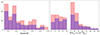 |
Fig. 1. Cluster redshift and |


The cluster member selection for the sample used in this work was developed by Sereno et al. (2025) using the CLEAN method (fully described in Mamon et al. 2013; see Appendix B of that paper), which is based on galaxy location in the PPS. So, the radial velocities of cluster members are the same as used in Sereno et al. (2025), who based their analysis on the Sloan Digital Sky Survey (SDSS) DR18, the Dark Energy Spectroscopic Instrument (DESI) databases, and the NASA/IPACExtragalactic Database (NED), in addition to some private catalogues and proprietary data. Moreover, we added new spectroscopic observations1 for three CHEX-MATE clusters, PSZ2 G113.91−37.01, PSZ2G046.10+27.18, and PSZ2G083.29−31.03, all of which are in the redshift range 0.37 < z < 0.41. We observed galaxies in these fields at the 10.4 m Gran Telescopio Canarias (GTC) telescope with the Optical Spectrograph and InfraRed Imager System (OSIRIS) in multi-object observing mode acquiring 2400 s exposures and two mask configurations for each cluster. For more details on the instrumental setup, data reduction process, and redshift estimates, see Ferragamo et al. (2020) and Aguado-Barahona et al. (2022). The procedures applied in this work are exactly the same as those used there. So, we obtained radial velocities for 80, 61, and 66 cluster members, respectively, with a precision of about 70 km s−1. These spectroscopic observations are limited, showing magnitude limits of r′∼21.5, and low sample completeness, below 30% within r500.
For these three clusters, we selected members by applying a 2.7σ clipping in the phase-space to minimise the fraction of interlopers2 (Mamon et al. 2010). However, we find that only PSZ2G046.10+27.18 has more than N = 50 members within the estimated r200. From here on, we refer to rap, 200 as the radius provided by the CLEAN procedure, to distinguish it from the values obtained by the MG-MAMPOSST fit.
In summary, including the GTC observations, we created 77 catalogues of cluster member galaxies (one for each cluster), with a total of 17 521 radial velocities, i.e. a mean of about 220 members per cluster. Of these, 75 clusters have been found to have N ≥ 50 confirmed members within the aperture radius R = rap, 200, after the application of the CLEAN algorithm (Sereno et al. 2025). In Fig. E.1 we plot the number of cluster members identified within R = rap, 200 after the cleaning as a function of the aperture velocity dispersion σap, 200 estimated by Sereno et al. (2025). Considering this spectroscopic dataset, we present in the following sections our procedure to analyse the main kinematical and dynamical properties of the CHEX-MATE cluster sample.
3. Kinematics analysis setup
We inferred the cluster mass profiles of the CHEX-MATE sample by employing the MG-MAMPOSST method (Pizzuti et al. 2023), which is based on the MAMPOSST (Mamon et al. 2013) algorithm to simultaneously recover the (total) gravitational potential and the orbit anisotropy profile of clusters from kinematic analyses of their member galaxies.
MAMPOSST is based on the assumption that the system is spherically symmetric and that galaxies are collisionless tracers of the gravitational potential. In this case, the dynamics is determined by the so-called (spherical) Jeans equation:
 (1)
(1)
where r indicates the 3D radial distance from the cluster centre, ν(r) is the number density profile of galaxies, σr2 is the velocity dispersion along the radial direction, and Φ is the total gravitational potential. The quantity β ≡ 1 − (σθ2 + σφ2)/2σr2 is the velocity anisotropy, with σθ2, σφ2 the velocity dispersion components along the tangential and azimuthal directions, respectively. In spherical symmetry, we have σθ2 = σφ2.
MAMPOSST and MG-MAMPOSST work in the so-called PPS, i.e. R, vlos, where R is the projected radial distance from the cluster centre – defined to be at the peak of the projected X-ray emission (Sereno et al. 2025) – and vlos is the LOS velocity of each galaxy, computed in the rest frame of the cluster. Given as input the parametric expressions of the gravitational potential, the number density profile, and the velocity anisotropy profile, the code implements a maximum likelihood fit to determine the best set of parameters describing the PPS distribution of cluster members.
MG-MAMPOSST extends the gravitational potential models available in the original MAMPOSST, further including generalised models of the velocity anisotropy profile, which we explore here. MG-MAMPOSST also includes popular modified gravity and alternative dark energy scenarios (see Pizzuti et al. 2021 for a description of the physics), viable at the cosmological level, which we do not analyse in this paper. Moreover, a recent update of the code implemented a module to include data of the velocity dispersion of the brightest cluster galaxy (BCG) in the fit, when available. Inclusion of the BCG velocity dispersion would allow the method to provide tight constraints on the slope of the dark matter profiles in clusters (see Biviano et al. 2023). However, in this work, we did not use the BCG module.
Therefore, we only considered galaxies outside of a minimum projected radius Rmin = 0.05 Mpc. The central region was excluded to avoid contamination by the BCG, which dominates cluster dynamics at very small radii. Furthermore, in its current implementation, MG-MAMPOSST assumes negligible streaming motions and a Gaussian 3D velocity distribution of the tracers.
We ran MG-MAMPOSST over our CHEX-MATE subsample of 75 clusters, which includes members up to a maximum projected radius  . Here
  is the estimate of the (dynamical) virial radius, either from the analysis of Sereno et al. (2025, rap, 200) or from the velocity dispersion (see Sect. 5 in Barrena et al. 2024) for those clusters for which the former is not available. This definition of maximum radius for cluster membership is a common choice to ensure the validity of the Jeans equation, as r200 is close to the virial radius which determines the region where the assumptions of Eq. (1) aresatisfied.
We sampled the parameter space with a Markov chain Monte Carlo (MCMC) Metropolis-Hastings algorithm for 110 000 points, considering the first 10 000 as the burn-in phase. Our final chain contains 100 000 samples for each run; this number has been chosen has a reasonable value to save computational time while ensuring convergence. In more detail, we checked convergence by considering the four clusters with the fewest members (N < 60) within rap, 200; and running n = 5 test chains for each of them. We then computed the corresponding Gelman-Rubin diagnostic coefficients  Gelman & Rubin (1992)3 checking that the requirement
  is always satisfied, as done in Pizzuti et al. (2024).
For the main analysis, a total of eight MG-MAMPOSST chains were generated per cluster in the sample. We explored combinations of two models for the number density distribution and four models for the total mass profile. The first, the Navarro-Frenk-White (NFW), model can be written as
 (2)
(2)
where M200 = 200 (H2(z)/2G) r2003 is the enclosed mass at r200 and c200 = r200/r−2 is the concentration, with r−2 being the radius at which the logarithmic slope of the density profile is −2. For the NFW model, this radius corresponds to rs.
The Hernquist profile has a steeper decline of the density at large radii, and the mass enclosed in a radius r reads (Hernquist 1990)
 (3)
(3)
where rs = 2 r−2.
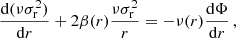
The Burkert model (Burkert 1995) has a central core in the density distribution, and the mass is given by
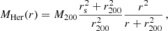
![Mathematical equation: $$ \begin{aligned} \begin{aligned}&M_{\rm Bur}(r) = \\&\frac{M_{200}\left[\mathrm{ln} \left((r/r_{\rm s})^2+1\right)+2 \mathrm{ln} (r/r_{\rm s}+1)-2 \tan ^{-1}(r/r_{\rm s})\right]}{\left[\mathrm{ln} \left((r_{200}/r_{\rm s})^2+1\right)+2 \mathrm{ln} (r_{200}/r_{\rm s}+1)-2 \tan ^{-1}(r_{200}/r_{\rm s})\right]}\,,\\ \end{aligned} \end{aligned} $$](/articles/aa/full_html/2025/07/aa55417-25/aa55417-25-eq13.gif) (4)
(4)
with rs ≃ r−2/1.5.
Finally, the Einasto model Einasto (1965) can be written as
![Mathematical equation: $$ \begin{aligned} M_{\rm Eis}(r) = M_{200}\frac{\gamma \left[\frac{3}{m}, \frac{2}{m}\left(\frac{r}{r_s}\right)^m\right]}{\gamma \left[\frac{3}{m}, \frac{2}{m}\left(c_{200}\right)^m\right]}, \end{aligned} $$](/articles/aa/full_html/2025/07/aa55417-25/aa55417-25-eq14.gif) (5)
(5)
where we set the shape parameter4m = 3 and rs = r−2 as for the NFW profile. Therefore, all models are described by two free parameters, the mass M200 (or equivalently, the radius r200) and the scale radius rs, which will be fitted within the MG-MAMPOSST algorithm.
As mentioned above, we further considered two models for the number density profile: the projected NFW (pNFW) and the projected Hernquist (pHer). These models are defined as the integral of Eqs. (2) and (3) along the LOS. While the profiles are characterised by two free parameters, only the scale radius rν5 is relevant in the analysis, as the other factors out in the solution of the Jeans equation implemented in MG-MAMPOSST. Note that for rν, we first performed a preliminary fit to the member galaxy distribution in the phase space, which does not require the binning of data (Sarazin 1980), assuming a constant completeness of the sample in the projected radial distance explored. This last assumption is rather strong, since our dataset exhibits incomplete and inhomogeneous spatial distributions; however, we carried out a detailed analysis on a few clusters to check that reasonable variation of the completeness does not provide relevant changes in the reconstructed mass profile. We then used the 95% confidence level (CL) limits of the inferred rν as the upper and lower bounds for the flat prior range in the MG-MAMPOSST fit (see below). We further verified that varying this interval produces negligible effects in the reconstructed mass profile.
As for the velocity anisotropy profile, we adopted a generalised Tiret (gT) model (see Mamon et al. 2019), which is an extension of the Tiret profile (Tiret et al. 2007) and is able to capture a broad ranges of possibilities for the orbits of member galaxies in clusters:
 (6)
(6)
where β0 and β∞ are the inner and outer values of the anisotropy, respectively, and rβ is a characteristic scale radius. In all cases, we set rβ = r−2 (i.e. the scale radius of the mass profile) as suggested by numerical simulations (Mamon et al. 2010). In MG-MAMPOSST, we worked with the rescaled parameters 𝒜0, ∞ = (1 − β0, ∞)−1/2, which are equal to one for completely isotropic orbits.
We adopted flat priors on all the fitted parameters, r200/Mpc ∈ [0.5, 5.0], rs/Mpc ∈ [0.04, 4.0], 𝒜0, ∞ ∈ [0.4, 7.0], rν ∈ [rνlow, rνup], where the last range is between the 95% lower and upper limits from the external fit of the projected number density distribution. Except for rν, the priors are non-informative.
For each posterior, we applied the Bayesian information criterion (BIC; see e.g. Mamon et al. 2019) to quickly select the best model among the eight combinations analysed:
 (7)
(7)
where k is the number of free parameters, N the number of data points, and ℒ the likelihood at the best fit. Generally, a model is said to be strongly preferred when its BIC is lower by a factor of ∼6 with respect to the others. For the models with the same number of free parameters, the BIC comparison is equivalent to the chi-square χ2 comparison. It is important to stress that MG-MAMPOSST only indicates which model is favoured relative to the others, but not the best model in an absolute sense. We further quantified the systematics induced by the modelling as half of the maximum variation between all the best-fit values of each parameter.
4. Results
Here we present the main outcomes from the MG-MAMPOSST analysis for the CHEX-MATE sample of 75 clusters. Among the mass profile models assumed, all of them adequately fit the PPS distribution, with the NFW profile performing better for 45% of the clusters, followed by Burkert (32.5%), Einasto (12.5%), and Hernquist (8%). This distribution may indicate a slight preference towards steeper central profiles with respect to those with cores. While it is true that the presence of interlopers that survived the CLEAN procedure can produce a steeper profile, thus biasing in favour of NFW-like models, the statistical significance of this is generally negligible, with a very small ΔBIC (≲1.0 on average). In contrast, the fits to the number density distribution of galaxies notably prefer the projected Hernquist model compared to the NFW model for more than 70% of the analysed clusters, with several cases where ΔBIC ≳ 6.0. This preference seems to be in contrast to other studies (e.g. van der Burg et al. 2016), which indicate a preference of the pNFW model. However, one should note here that the assumption of a constant completeness may play a significant role. Indeed, while it is true that the constraints on a mass profile distribution are not strongly affected by the choice of the model of the number density profile in the MG-MAMPOSST fit, the slope of ν(r) and the value or the scale radius rν depends on the completeness. In order to deal with this issue, one should compute the completeness, cluster by cluster, by comparing photometric and spectroscopic catalogues. However, this analysis is beyond the scope of the paper. As an example, we considered the case of the cluster PSZ2 G049.22+30.8, for which the completeness as a function of the projected radius has been estimated according to the model
 (8)
(8)
with A = 0.817, B = −0.413. While in this case the best-fit projected number density is always a NFW profile, the value of the scale radius changes from  when accounting for the correct completeness, to
  , when a constant completeness is assumed (uncertainties are given at the 95% CL).
In Table A.1 we report the regression results. In the second and third columns, we list the best-fit models (i.e. the models that give the highest posterior) for mass and density, respectively. For each entry, the first uncertainties refer to the (statistical) 95% confidence intervals, while the second values are the systematic uncertainties computed as discussed above. The last four columns show the value of the log posterior lnP of the best fit, the cluster redshift z, the value of the Anderson-Darling coefficient A2 (see Sect. 4.3), and the estimated LOS velocity dispersion at r200, σap, 200. Note that the MG-MAMPOSST procedure is robust in estimating r200 against the choice of the mass, anisotropy and number density models, as shown by the small systematic uncertainties compared with the statistical errors.
In Fig. 2 we show an example of the mass and anisotropy profiles obtained from MG-MAMPOSST for one rich cluster (Ngal = 291 spectroscopic members within rap, 200) in the sample, PSZ2 G067.17+67.46. The mass is parametrised as an NFW model, which gives the best-fit profile, with a pNFW model for the number density of the member galaxies.
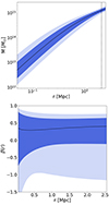 |
Fig. 2. Mass profile (top) and radial velocity anisotropy profile (bottom) of the cluster PSZ2 G067.17+67.46, as obtained via the MG-MAMPOSST analysis with Ngal = 299 galaxies and adopting a NFW model and a gT model, respectively. In both plots, darker and lighter shaded regions refer to 68% and 95% CLs, respectively. The vertical dashed line in the top panel identifies the best fit for r200 = 2.19 Mpc. |
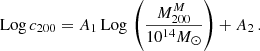
We then computed the mass inside the virial radius as M200 = (100 H2(z)/G)×r2003, and we performed a first comparison with the results of Sereno et al. (2025). Figure 3 displays the values of Log M200 as obtained by MG-MAMPOSST (vertical axis), and Log Mσ, 200c estimated from the aperture velocity dispersion σap, 200 with the method of Sereno et al. (2025, horizontal axis). The superscript (M) refers to the MG-MAMPOSST estimates.
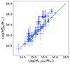 |
Fig. 3. Scatter plot of Log M200, inferred from the kinematic analysis with MG-MAMPOSST (vertical axis), and Log Mσ, 200c obtained by Sereno et al. (2025, horizontal axis). The error bars represent the 68% CL, and the dashed black line the bisector. Darker points highlight those clusters for which Log (M200M/Mσ, 200c) > 0.3. |
The results show an overall good agreement among the two estimates, confirming the robustness of the simpler analytical approach of Sereno et al. (2025). However, for seven clusters MG-MAMPOSST tends to overestimate M200 with respect to the findings of Sereno et al. (2025). For those clusters we find an average logarithmic difference Log M200M − Log Mσ, 200c > 0.3 dex. If we look at the relation between  and the aperture velocity dispersion σap, 200 (Fig. 4) obtained by Sereno et al. (2025) using the CLEAN method (Mamon et al. 2013), it is easy to see that six of the seven clusters are characterised by large values of σap, 200 > 103 km/s. This pattern suggests that clusters in the CHEX-MATE sample with very large velocity dispersions suffer a stronger contamination of interlopers. This fact was first found by Mamon et al. (2010) who, working with simulated halos, found that the fraction of interlopers should be (slightly) more important in the more massive halos since they have (slightly) lower concentrations (Navarro et al. 1997; Macciò et al. 2008) and they typically live in richer environments. That is, the larger fraction of interlopers that survived the membership selection performed by Sereno et al. (2025) in high-mass clusters could translate into a higher mass estimation by MG-MAMPOSST – which is a more complex model with respect to that of Sereno et al. (2025) – for the most massive systems.
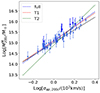 |
Fig. 4. Logarithm of the aperture velocity dispersion within R = r200, σap, 200 compared to the logarithm of M200M estimated from MG-MAMPOSST. The bars refer to 68% uncertainties. The blue line indicates the best-fit linear model of Eq. (9) when z = 0.2. The solid black line identifies the σ ∝ M3 relation. |
Moreover, in MG-MAMPOSST the concentration c200 = r200/r−2 is a free parameter (or better, it is a quantity derived from two parameters optimised within the fit), while in Sereno et al. (2025) it is fixed as a function of r200 using the concentration–mass relation proposed by Diemer & Joyce (2019). As shown by the blue points in Fig. 8, the off-trend clusters are characterised by a concentration estimated by MG-MAMPOSST that is lower than the prediction of Diemer & Joyce (2019, solid brown line), consequently boosting the reconstructed M200.
The blue line in Fig. 4 shows the best orthogonal distance regression (ODR) fit for the linear model
 (9)
(9)
when fixing the redshift to the pivot value of the sample zp = 0.2; in Eq. (9), Fz = H(z)/H(zp). We find
 (10)
(10)
which is slightly steeper than α ∼ 3, the value reported in, for example, Munari et al. (2013) and Ferragamo et al. (2020). If we consider the T1 and T2 clusters separately, the ODR fit of Eq. (9) provides a slightly lower αT1 = 3.31 ± 0.17 for the T1 sample – close to the ∼σ3 relation and a higher value αT2 = 4.81 ± 0.64 for T2. This reflects the fact that T2 contains massive clusters by construction, and that among the seven off-trend objects, five belong to T2. The best ODR fits for zp are shown as the dashed red and green lines for T1 and T2, respectively.
4.1. Comparison with SZ mass estimates
To compare our kinematic masses with the ones obtained from the SZ effect, we further derived the distribution of M500 = 500 H2(z)/(2G)×r5003, as follows: for each value of r200, rs in the MCMC chain we obtained the corresponding parametric mass profile M(r|r200, rs). The radius r500 is then given by the numerical solution of the equation
 (11)
(11)
From that, the computation of M500 is straightforward.
In Fig. 5 we plot the values of Log M500 as obtained by MG-MAMPOSST (vertical axis) and inferred by SZ (horizontal axis), where the superscript (M) and (SZ) refers to the MG-MAMPOSST and SZ estimates, respectively. We find a strong correlation between the two estimates (Pearson coefficient r = 0.68, p-value < 10−5); we fitted the linear relation
 (12)
(12)
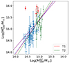 |
Fig. 5. Scatter plot of M500 inferred from the SZ effect by Planck (on the vertical axis) and from the kinematic analysis with MG-MAMPOSST (horizontal axis). The error bars represent the 68% CL, and the red points show those clusters for which the logarithmic difference (δη) is larger than 0.8 dex. Dark green points highlight clusters belonging to T2. The purple line is the ODR fit that considers all the clusters, while the blue one is the linear fit done by discarding the four outliers. The best-fit (with the outliers removed) linear models for T1 and T2 are shown separately with the dashed red and dark green lines, respectively. |
where the mass-dependent bias (1 − B) is defined similarly to that done, for example, in Ferragamo et al. (2021) and Aguado-Barahona et al. (2022). This way, the usual bias  is recovered when αSZ = 1.
We obtain αSZ = 0.84 ± 0.05, and an overall mass-dependent bias Log(1 − B) = − 0.18 ± 0.06 dex when all the galaxy clusters in the sample are considered, corresponding to (1 − B) = 0.67 ± 0.09; this means that the kinematic results from MG-MAMPOSST produce larger masses with respect to those derived from the Planck SZ signal. This value seems to be in agreement within errors with those obtained by Planck Collaboration VI (2020) and Lesci et al. (2023) from Baryon acoustic oscillation and 3D clustering of the PSZ2 clusters. In addition, our estimate is similar to that found by the fit of Sereno et al. (2025), although slightly larger than that of Ferragamo et al. (2021) and Aguado-Barahona et al. (2022), who obtained a bias of (1 − B)∼0.80 comparing Planck SZ-X-ray calibrated masses of 270 PSZ1 and 388 PSZ2 clusters, respectively, with the kinematic mass estimated through the total velocity dispersion. When forcing αSZ to unity, however, the difference between the two mass estimates is even larger, almost doubled: (1 − B1) = 0.43 ± 0.08, which is not consistent with the abovementioned works.
It is interesting to note that the sample includes a few clusters for which the kinematic mass is about one order of magnitude larger than the one given by the SZ proxy. We mark the four clusters for which
 (13)
(13)
as red points in Fig. 5. However, the PPS distributions of those clusters show evident sign of a disturbed dynamical state, as displayed in the left plots of Fig. B.1, with very large velocity dispersions and presence of possible important structures that are not part of the main cluster, as in the case of PSZ2G056.77+36.32, and PSZ2G040.03+74.95.
The disturbed dynamical state of these four clusters is further indicated by the distributions of the velocities along the LOS (central plots of Fig. B.1); those for PSZ2G056.77+36.32 and PSZ2G040.03+74.95 exhibit noticeable bimodal distributions. This is further indicated by relatively large values of the Anderson Darling coefficient, A2 – a measure of the degree of un-relaxation that is discussed in Sect. 4.3 – for three of the four outliers. Note that here we considered the members selected by running the CLEAN algorithm in its default settings, which do not employ an identification of substructures. However, as already done in Sereno et al. (2025), a refined analysis can be performed to study these systems. In more detail, PSZ2G040.03+74.95 (also known as Abell 1831) has been already identified as a double system: it is made of two clusters, A and B at z = 0.063 and 0.076, respectively, nearly aligned along the LOS, as discussed in Sereno et al. (2025). A similar situation holds for the object PSZ2G218.81+35.51 (see Sereno et al. (2025) and also the histogram of the LOS velocities in Fig. 6). We find a logarithmic difference δη = 0.68 ± 0.42 for PSZ2G218.81+35.51, where the large uncertainties reflect the inefficiency of MG-MAMPOSST in fitting the double system with a single mass model.
 |
Fig. 6. LOS velocity distribution for the system PSZ2G218.81+35.51, made of two separate clusters, as mentioned in Sereno et al. (2025). |
By considering the two sub-groups in PSZ2G040.03+74.95 and PSZ2G218.81+35.51 as independent clusters6, the kinematical analysis gives M200 < 7 × 10¹⁴ M⊙ and  for PSZ2G040.03+74.95 A, B, and
  ,
,  for PSZ2G218.81+35.51 A, B. Note that for PSZ2G040.03+74.95 A we are only able to set an upper limit with MG-MAMPOSST, given the small number of members considered in the fit (only 25 members lie within R = r200, well below the limit of 50 we imposed on the full sample) and the relatively small σap, 200 = 461 km s−1, compared to the error in the LOS velocities. It is important to mention that the results for these bi-modal systems are in agreement (albeit with larger uncertainties) with the values obtained by the simple halo model of Sereno et al. (2025).
For the most massive sub-components in the bimodal clusters (which are identified as the CHEX-MATE clusters; see Sereno et al. (2025) and references therein), the logarithmic difference is now reduced to δη = 0.8 ± 0.3 (PSZ2G040.03+74.95) and δη = 0.15 ± 0.11 (PSZ2G218.81+35.51), instead of 1.4 and 0.68. These interesting cases, as well the other three clusters mentioned above, deserve a separate detailed analysis of their properties. Such an analysis is beyond the scope of this paper and it will be performed in a separate work. We consider only the main sub-components of the double systems in the forthcoming analyses.
If we remove the four clusters with large δη and fit Eq. (12) again (dashed blue line in Fig. 5), we remarkably find a negligible mass-dependent bias within the uncertainties Log(1 − B) = 0.02 ± 0.04, which corresponds to 1 − B = 1.04 ± 0.09, with a slightly flatter slope αSZ = 0.71 ± 0.04. Note that, however, the bias is still large when fixing the slope to 1, 1 − B1 = 0.54 ± 0.11, from which we can conclude that kinematic mass estimates are a factor of two larger, on average, with respect to SZ probes. Note that this value is now in agreement with the findings of, for example, Lesci et al. (2023). Here we have ignored the possible redshift dependence of the sample and neglected the Malmquist bias, both were already considered in Sereno et al. (2025). SZ masses are biased high, which can produce an underestimation of B. When considering T1 and T2 separately (after removing the four biased clusters), the fit is still consistent with a negligible mass-dependent bias: (1 − B) = 1.12 ± 0.13 for the former and (1 − B) = 1.32 ± 0.44 for the latter. The larger uncertainties in T2 reflect a wide scatter in δη, as shown by the green points in Fig. 5. For B1, we find (1 − B1) = 0.64 ± 0.04 for T1 and (1 − B1) = 0.40 ± 0.04 for T2.
Note that δη does not exhibit a strong correlation with redshift (see Fig. 7), with a scattered distribution. However, if we compute the fraction of galaxies with δη > 0.5 in two redshift bins, z < 0.2 and z > 0.2, we find 0.14 and 0.28, respectively. This difference should not come as a surprise, since clusters with z > 0.2 belong to the T2 selection, which contains massive clusters by construction (thus characterised by larger velocity dispersions; see e.g. Sereno et al. 2025). Those clusters exhibit overall larger discrepancies between  and
and  , attributed to a potentially stronger contribution of interlopers in the kinematics analysis, as already mentioned above, in clusters with high velocity dispersions.
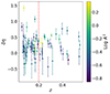 |
Fig. 7.
|
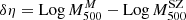
4.2. Concentration–mass relation
In Fig. 8 we plot the relation between c200 and M200 of the sample, as derived by the MG-MAMPOSST analysis. For the two double systems, PSZ2G056.77+36.32 and PSZ2G218.81+35.51, we considered the sub-components separately and ended up discarding PSZ2G056.77+36.32 A, given its limited statistics. Although the points appear quite scattered and have large uncertainties, a mild, positive correlation can be observed (Spearman rank coefficient 0.33, corresponding to a p-value of 2 × 10⁻³). For a quantitative analysis, we performed a Bayesian regression. We followed the CoMaLit (Comparing Masses from Literature) scheme described in Sereno & Ettori (2015b,a, 2017) and Sereno et al. (2015a), which we refer to for details, and implemented in the R-package LIRA (Sereno 2016)7.
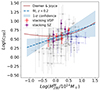 |
Fig. 8. Concentration–mass relation for the CHEX-MATE sample. The error bars indicate 68% uncertainties in the parameters; we highlight in light blue the clusters with |
The mass–concentration relation is modelled with a linear relation in log-space, similarly to Eq. (9),
 (14)
(14)
where Fz = H(z)/H(zref) is the redshift-dependent Hubble parameter normalised to the reference redshift of the sample, zref = 0.2, and Mpivot = 1015 M⊙ is the pivot mass. The concentration at the reference mass and redshift is given by c200, ref = 10αC.
Statistical biases and correlation effects have to be carefully dealt with (Sereno et al. 2015b). For our analysis, we assumed that both  , that is, the covariate in Eq. (14), and Y = Log(c200), that is, the response, are intrinsically scattered with respect to the true mass, Z, whose distribution we modelled as a Gaussian with a redshift-dependent mean and variance (Sereno & Ettori 2015a). We assumed that the covariate is scattered but unbiased with respect to the true mass. We considered heteroscedastic and correlated uncertainties for mass and concentration. For central location and scale, we considered the bi-weight estimators (Beers et al. 1990). We applied non-informative priors (Sereno & Ettori 2015a, 2017): the uniform distribution for αC and the mean of the distribution of Z; the Student’s t1 distribution with one degree of freedom for the slopes βC and γC; and the Gamma distribution for the inverse of either variances or intrinsic scatters.
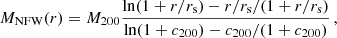
The regression favours a flattening and upturn of the relation at large masses, in agreement with theoretical predictions (Diemer & Joyce 2019). The best-fit values of the linear relation are
 (15)
(15)
To test the robustness of the results on the regression scheme, we also fitted the relation with a simple linear model, similarly to that done, for instance, in Biviano et al. (2017), using the ODR method and neglecting the redshift dependence,
 (16)
(16)
We find A1 = 0.27 ± 0.08, A2 = 0.20 ± 0.11, which confirms the trend of rising concentration for high mass clusters. The same is valid if we fit the T1 and T2 clusters separately, in particular A1T1 = 0.35 ± 0.12 and A1T2 = 0.21 ± 0.14. Our findings might appear to be in tension with other theoretical expectations (e.g. Dutton & Macciò 2014; Ragagnin et al. 2020) and observational determinations of the c − M relation (see e.g. Merten et al. 2015 and Biviano et al. 2017; the latter study is also based on the MG-MAMPOSST technique). However, this statement should be considered cautiously. The CHEX-MATE sample covers the very massive end of the halo mass function at intermediate redshifts, where the upturn is visible. Selection effects as well as the uncertainties in the kinematic analysis can play a significant role; in particular, X-ray- and SZ-selected samples tend to favour more centrally concentrated and relaxed clusters, biasing the inferred c-M relation upwards (e.g. Meneghetti et al. 2014). Moreover, as mentioned before, the presence of residual interlopers may affect the high-mass end of the sample, giving rise to the observed trend.
4.3. Substructures and un-relaxation
To further investigate the overall kinematical state of the cluster sample, we computed the Anderson-Darling coefficient A2 (Anderson & Darling 1952), which measures deviation from Gaussianity of the LOS velocity distribution, which is a good indicator of the dynamical state of a cluster (e.g. Roberts et al. 2018). Large values of A2 have been shown to be associated with deviations from relaxation (e.g. Pizzuti et al. 2020; Barrena et al. 2024). The colours of each point in Fig. 7 indicates the corresponding value of the (logarithm of the) Anderson-Darling coefficient, computed using all galaxies within R = rap, 200c as given by CLEAN (Sereno et al. 2025). Note that three of the four outliers with δη > 0.8 are characterised by large values of A2 = 0.64, 0.87, and 4.63 for PSZ2G056.77+36.32, PSZ2G008.31-64.74, and PSZ2G040.03+74.95. Note that for PSZ2G056.77+36.32 the group below vz = −2000 km/s is at large radii from cluster centre (see the top left plot of Fig. B.1), and thus is not considered in the computation of the Anderson-Darling coefficient. If all galaxies in the phase space are included, we find A2 = 2.49 While PSZ2G075.71+13.51 exhibits a low value A2 = 0.21, the velocity distribution is negatively skewed (s ∼ −0.11) with a further negative excess of kurtosis (k − 3 = −0.43).
No strong correlations can be highlighted among A2 and δη, but dividing again the sample into two subsamples according to the median value A2 = 0.44, the average logarithmic differences in the two bins, computed by 1000 bootstrap resampling, are ⟨|δη|⟩ = 0.23 ± 0.08 and 0.13 ± 0.07 for A2 > 0.44 and A2 < 0.44, respectively. This small difference in mean |δη| shows a weak preference of lower biases for clusters with a more regular LOS velocity dispersion.
The MG-MAMPOSST method may be sensitive to the presence of relevant substructures in clusters, which are connected to recent merging activity and thus indicate a possible disturbed dynamical state (e.g. Wen & Han 2013; Parekh et al. 2015; Kimmig et al. 2023). Thus, we searched for possible correlations between the number of substructures in the cluster and the observed logarithmic difference, δη. We estimated the fraction of galaxies in substructures, fsub, over the total number of galaxies within R = r200 by means of the DS+ method8 from Benavides et al. (2023). This DS+ method extends the original algorithm of Dressler & Shectman (1988) for the identification of sub-groups in clusters by looking for galaxy clumps whose mean velocities and dispersion deviate from the global cluster values. DS+ employs a combination of projected position and LOS velocities to identify substructures and estimate the probability of each galaxy belonging to each of those groups.
For each cluster, we ran 1000 Monte Carlo simulations and we a p-value of 0.01 as the threshold for the identification of a substructure (see also Barrena et al. 2024). We worked in the so-called non-overlapping mode, i.e. each galaxy is attributed to at most one group. We then defined fsub = Nsub/N200, where Nsub is the total number of galaxies in all the substructures found by DS+, and N200 is the number of members in the projected cylinder R < r200. In Fig. 9 the distribution of δη as a function of fsub is shown, colour-coded according to the values of A2. Again, no relevant trends can be drawn from the sample, with a more scattered distribution across the range of fsub. It is worth pointing out that a δη close to zero does not indicate that the cluster mass estimations are unbiased, but it may suggest that the SZ and kinematic masses are biased towards the same direction. Figure 10 further shows the relation between fsub and Log A2. It is evident that, despite the correlation not being strong (Pearson coefficient r = 0.43), a trend of having large A2 for large values of fsub is present.
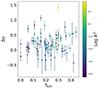 |
Fig. 9.
|
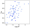 |
Fig. 10. Fraction of galaxies in substructures, fsub, as a function of the logarithm of the Anderson-Darling coefficient, A2. The darker stars indicate the clusters for which Log (M200M/Mσ, 200c) > 0.3. |
A more accurate analysis would involve masses estimated from WL, as well as the combination of different morphological parameters (e.g. those derived from X-ray analyses; see Campitiello et al. 2022) to have a clearer indication of the equilibrium state of the clusters. This will be the subject of follow-up work.
5. Orbits of galaxies as a function of mass and redshift
The orbital anisotropy of member galaxies in clusters is one of the key quantities in kinematic analyses. It has been shown that the nature of anisotropy can be linked to the dynamical state of the cluster and its formation history (e.g. Mamon et al. 2019); in general, studies of observed clusters and cluster-size halos in cosmological simulations have identified an overall trend of isotropic orbits in the cluster core, and an increasing radial anisotropy towards the outskirts. Moreover, galaxies of different morphological types in clusters exhibit different orbital behaviours. In particular, early-type galaxies that are believed to have fallen into the cluster at early times may prefer more isotropic orbits, while spiral galaxies are thought to follow fairly radial paths (e.g. Munari et al. 2014; Mamon et al. 2019; Biviano et al. 2024). The reconstruction of anisotropy profiles in clusters is generally a complicated issue; this is because β(r) is not a direct observable and it is degenerate with the total mass (Binney & Mamon 1982), constituting a possible source of systematic error in the reconstruction of dynamical mass profiles. To address this, both parametric approaches (e.g. Mamon et al. 2013; Read et al. 2021) and non-parametric methods (see e.g. Mamon et al. 2019 andreferences therein) have been developed. The MG-MAMPOSST technique (as does the original MAMPOSST) relies on a joint parametric modelling of both mass and anisotropy profiles, which has been shown to work robustly and adequately well in a wide range of cases (Mamon et al. 2013; Pizzuti et al. 2020; Biviano et al. 2023). However, the uncertainties in the reconstructed radial profile β(r) are large for a single cluster, even for a considerably large number of members in the MG-MAMPOSST fit (see the example of PSZ2 G067.17+67.46 in the bottom plot of Fig. 2, with Ngal = 299 galaxies used in the analysis).
This issue can be solved in two ways. One possibility is to assume prior constraints on the mass profile, as provided, for example, by hydrostatic equilibrium or WL analyses (e.g. Annunziatella et al. 2016; Aguerri et al. 2017). On the other hand, one can infer information on the anisotropy profile as a function of cluster mass and redshift by populating the PPS with a stacking procedure. We adopted the latter approach and performed two different stacking procedures. First, we identified clusters with similar velocity dispersions in two redshift bins, namely z ≤ 0.2 and 0.2 < z < 0.6 (which mostly splits clusters into the T1 or the T2 subsample). In the first bin, we further divided the clusters into three sub-bins of velocity dispersion, centred on ![Mathematical equation: $ \sigma_{\mathrm{ap,200}}/[\mathrm{km\,s}^{-1}] = 750,\, 980 $](/articles/aa/full_html/2025/07/aa55417-25/aa55417-25-eq39.gif) , and 1360, respectively. We then generated the three stacked clusters (one for each bin of σap, 200) by considering all the member galaxies of CHEX-MATE clusters belonging to the same bin. The choices of the bins and the construction ensure that each stack contains N ∼ 3000 galaxies. For the high-redshift bin, we end up with only two stacked clusters, with
, and 1360, respectively. We then generated the three stacked clusters (one for each bin of σap, 200) by considering all the member galaxies of CHEX-MATE clusters belonging to the same bin. The choices of the bins and the construction ensure that each stack contains N ∼ 3000 galaxies. For the high-redshift bin, we end up with only two stacked clusters, with ![Mathematical equation: $ \sigma_{\mathrm{ap,200}}/[\mathrm{km\,s}^{-1}] = 1040, 1600 $](/articles/aa/full_html/2025/07/aa55417-25/aa55417-25-eq40.gif) .
.
The second stacking has been performed considering five bins for clusters with similar SZ–X-ray calibrated masses – three for z < 0.2,  M⊙ = 3.23, 5.48, 7.74, and two for z > 0.2,
  M⊙ = 7.91, 12.10. This second set is to consider a stacking criterion (
 ) that is independent of kinematic variables. As an example, the stacked PPS for this case are shown in Appendix C.
For each of the ten stacked clusters, we considered galaxies in the projected range [0.05 Mpc, 1.1 ⟨rap, 200⟩], where ⟨rap, 200⟩ is the average of rap, 200 over all the clusters in the bin. We applied the MG-MAMPOSST method assuming a NFW model for the mass distribution and a pNFW for the projected number density distribution; as before, we performed a MCMC sampling of the parameter space {r200, rs, rν, 𝒜0, 𝒜∞}, adopting the same flat prior listed in Sect. 3. Figures 11 and 12 show the radial profiles of the velocity anisotropy obtained from the MG-MAMPOSST analysis of the stacked clusters (σap, 200 and SZ, respectively) at z < 0.2 (top panels in each plot) and z > 0.2 (bottom panels in each plot). For the stacking in velocity dispersion, we see that all the profiles (except the one for the most massive cluster, σap, 200 ∼ 1600 km s−1) are consistent with central isotropic orbits within one σ, and with an increase in the anisotropy towards the cluster outskirts, as found by other studies in the literature (Mamon et al. 2019).
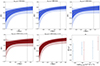 |
Fig. 11. Radial velocity anisotropy profiles for stacked clusters, where the stacking is in velocity dispersion. The bands show the 68% and 95% regions, and the black curve is the median profile. Top: z < 0.2. Bottom: z > 0.2. The bottom-right plot shows the value of β(r = r200) with 68% error bars (blue and red for z < 0.2 and z > 0.2, respectively). In all plots, the vertical dashed lines indicate the average rap, 200 in the corresponding velocity dispersion bin. |
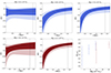 |
Fig. 12. Radial velocity anisotropy profiles for the stacked clusters, where the stacking is in bins of |


In the bottom-right panel, we can observe a slight, although not very significant, trend to have more radial orbits at the virial radius for clusters with a larger velocity dispersion. The most massive stacked cluster exhibits a more ‘extreme’ behaviour, passing from tangential orbits (β < 0) at the centre, to largely radial ones in the outskirts. However, this bin contains clusters with δη > 0.8, which, as we have discussed, are characterised by disturbed dynamical states. The same trend of increasing radial orbits at virial radius is found in terms of the SZ mass, as highlighted in Fig. 12. In this case, however, only the first mass sub-bins in each redshift cut (z < 0.2 and z > 0.2) exhibit a central anisotropy consistent with zero at the 68% CL, while the others are in agreement with no anisotropy at the 95% CL, with a slight preference for central tangential orbits that is not very statistically significant.
6. Conclusions
We have studied the kinematical and dynamical properties of 75 massive galaxy clusters of the CHEX-MATE sample for which high-precision spectroscopic measurements of LOS velocities and projected positions are available. By means of the MG-MAMOOSST code, we jointly reconstructed mass profiles and velocity anisotropy profiles for eight combinations of mass and number density models. We find that the NFW prescription is preferred by the kinematic analysis for about half of the sample; the second most preferred is the Burkert model. This confirms the assumptions of the halo model used in the dynamical mass determinations of Sereno et al. (2025). Moreover, the constraints on the virial radius r200 (and on the mass M200) are robust against variations in the mass and number density models, as shown by the relatively small systematic uncertainties (Table A.1).
We compared the masses obtained from the SZ–X-ray-calibrated signal, finding (1 − B1) = 0.54 ± 0.11 when clusters with evident disturbed dynamical states are removed. A negligible bias is instead obtained when fitting with a linear relation that allows for mass dependence, (1 − B) = 1.04 ± 0.09. When the clusters with a logarithmic mass difference δη > 0.8 dex (which are high-velocity dispersions σap, 200 > 1.4 × 10³ km/s) are also considered, an overall positive mass-dependent bias, (1 − B) = 0.67, is found. Note that SZ masses may be overestimated due to the Malmquist bias, as discussed in Sereno et al. (2025); this might affect our findings, leading to a larger value of (1 − B). A refined analysis is beyond the scope of the current work, but one is presented in Sereno et al. (2025). We investigated the concentration–mass relation and compared it to theoretical expectations. Byperforming a Bayesian linear regression by means of the LIRA package, we found weak evidence of a rising trend at high masses, as also predicted by the Diemer & Joyce (2019) model and recently found by Butt et al. (2025) via a kinematic analysis of the Hectospec Cluster Survey (HeCS) cluster sample. Interestingly, the results obtained for the sample of CHEX-MATE clusters are fully consistent with the prediction of the Λ cold dark matter scenario, given an average value of ⟨c200⟩ = 3.5 with a scatter of 1.8. The results of the various scaling relations investigated in this work are summarised in Table 1.
Results for the parameters of the linear fits of the relations discussed in this paper.
We studied the dynamical state of the clusters by comparing δη with two quantities that can be related with dynamical un-relaxation and disturbed morphology, namely the Anderson-Darling coefficient, A2, and the fraction of galaxies in substructures, fsub. No evident relations are found for A2 and fsub. Nevertheless, a lower averaged δη is obtained for clusters with A2 < 0.44 (0.44 being the median value of the sample). Note, however, that a more complete analysis should investigate the differences with the WL mass determinations and account for the X-ray morphology to better identify substructures and departures from equilibrium. This will be the subject of an upcoming work. Finally, we studied the shape of the radial velocity anisotropy profile by dividing the sample into two bins of redshift and collecting clusters within three and two sub-bins of σap, 200. We stacked clusters in the same bin and applied MG-MAMPOSST to those stacked systems to reconstruct the orbits from the centre to the edges. We performed a similar stacking procedure with bins of  , which are not directly related to the kinematical properties of the clusters. Consistent with the literature, orbits tend to be isotropic or tangential at the centre and more radial towards the edge of the clusters, where galaxies are thought to be falling into the cluster’s potential for the first time (Mamon et al. 2019). There is a slight trend towards increasingly radial orbits at r200 with larger σap, 200 (which, in turn, is connected to higher dynamical masses); we find the same trend with increasing
  .
.
More broadly, our results indicate that the most massive galaxy clusters at z < 0.6 are generally close to dynamical equilibrium. Nonetheless, we identify some cases where even the most massive systems appear to deviate from full virialisation. As previously mentioned, a comprehensive assessment of the dynamical state of the CHEX-MATE sample will be carried out in a forthcoming study, which will incorporate a more complete set of morphological and kinematic indicators, as well as a comparison with mass estimates from WL and X-ray data.
These new dataset will be made publicly available soon, but it is already available upon request. An extract can be found in Appendix D.
Galaxies not belonging to the clusters falling inside the PPS.
The Gelman-Rubin coefficient is defined as ![Mathematical equation: $ \hat{R} = [W(L-1)/L + B/L]/W $](/articles/aa/full_html/2025/07/aa55417-25/aa55417-25-eq51.gif) , where L is the length of the chains, B the variance of the means of the chains, and W the averaged variances of the individual chains across all chains.
, where L is the length of the chains, B the variance of the means of the chains, and W the averaged variances of the individual chains across all chains.
We checked that varying the exponent between m = 2 and m = 5 does not lead to statistically relevant changes in the final posterior.
We defined the scale radius of the number density profile as rν to avoid confusion with that of the mass profile.
The selection of members for the subsystems is performed as discussed in Sereno et al. (2025).
The package LIRA (LInear Regression in Astronomy) is publicly available from the Comprehensive R Archive Network at https://cran.r-project.org/web/packages/lira/index.html.
The code is freely available at https://github.com/josegit88/MilaDS.
Acknowledgments
This project has been partially funded by the Spanish Ministerio de Ciencia, Innovación y Universidades through the programme Generación del Concimiento 2021, with code PID2021-122665OB-I00. R. Barrena acknowledges support by the Severo Ochoa 2020 research programme of the Instituto de Astrofísica de Canarias. S.E., M.S., acknowledge the financial contribution from the contracts Prin-MUR 2022 supported by Next Generation EU (M4.C2.1.1, n.20227RNLY3 The concordance cosmological model: stress-tests with galaxy clusters). M.S. acknowledges financial contributions from INAF Theory Grant 2023: Gravitational lensing detection of matter distribution at galaxy cluster boundaries and beyond (1.05.23.06.17). S.E. acknowledges the financial contribution from the European Union’s Horizon 2020 Programme under the AHEAD2020 project (grant agreement n. 871158). DE acknowledges support from the Swiss National Science Foundation (SNSF) through grant agreement 200021_212576. C.P.H. acknowledges support from ANID through Fondecyt Regular project number 1252233, and from MILENIO - NCN2024_112. JS was supported by NASA Astrophysics Data Analysis Program (ADAP) Grant 80NSSC21K1571. BJM acknowledges support from Science and Technology Facilities Council grants ST/V000454/1 and ST/Y002008/1. GWP acknowledges long-term support from CNES, the French space agency. GC acknowledges the support from the Next Generation EU funds within the National Recovery and Resilience Plan (PNRR), Mission 4 – Education and Research, Component 2 – From Research to Business (M4C2), Investment Line 3.1 – Strengthening and creation of Research Infrastructures, Project IR0000012 – “CTA+ – Cherenkov Telescope Array Plus”. MD acknowledges the support of two NASA programs: NASA award 80NSSC19K0116/ SAO subaward SV9-89010 and NASA award 80NSSC 22K0476.
References
- Abell, G. O. 1958, ApJS, 3, 211 [NASA ADS] [CrossRef] [Google Scholar]
- Aguado-Barahona, A., Rubiño-Martín, J. A., Ferragamo, A., et al. 2022, A&A, 659, A126 [NASA ADS] [CrossRef] [EDP Sciences] [Google Scholar]
- Aguerri, J. A. L., Agulli, I., Diaferio, A., & Dalla Vecchia, C. 2017, MNRAS, 468, 364 [NASA ADS] [CrossRef] [Google Scholar]
- Amodeo, S., Mei, S., Stanford, S. A., et al. 2017, ApJ, 844, 101 [NASA ADS] [CrossRef] [Google Scholar]
- Anderson, T. W., & Darling, D. A. 1952, Ann. Math. Stat., 23, 193 [Google Scholar]
- Annunziatella, M., Mercurio, A., Biviano, A., et al. 2016, A&A, 585, A160 [NASA ADS] [CrossRef] [EDP Sciences] [Google Scholar]
- Barrena, R., Pizzuti, L., Chon, G., & Böhringer, H. 2024, A&A, 691, A135 [NASA ADS] [CrossRef] [EDP Sciences] [Google Scholar]
- Beers, T. C., Flynn, K., & Gebhardt, K. 1990, AJ, 100, 32 [Google Scholar]
- Benavides, J. A., Biviano, A., & Abadi, M. G. 2023, A&A, 669, A147 [NASA ADS] [CrossRef] [EDP Sciences] [Google Scholar]
- Binney, J., & Mamon, G. A. 1982, MNRAS, 200, 361 [Google Scholar]
- Biviano, A., & Katgert, P. 2004, A&A, 424, 779 [NASA ADS] [CrossRef] [EDP Sciences] [Google Scholar]
- Biviano, A., Moretti, A., Paccagnella, A., et al. 2017, A&A, 607, A81 [NASA ADS] [CrossRef] [EDP Sciences] [Google Scholar]
- Biviano, A., Pizzuti, L., Mercurio, A., et al. 2023, ApJ, 958, 148 [NASA ADS] [CrossRef] [Google Scholar]
- Biviano, A., Poggianti, B. M., Jaffé, Y., et al. 2024, ApJ, 965, 117 [Google Scholar]
- Burkert, A. 1995, ApJ, 447, L25 [NASA ADS] [Google Scholar]
- Butt, M. A., Haridasu, S., Diaferio, A., et al. 2025, arXiv e-prints [arXiv:2504.16685] [Google Scholar]
- Campitiello, M. G., Ettori, S., Lovisari, L., et al. 2022, A&A, 665, A117 [NASA ADS] [CrossRef] [EDP Sciences] [Google Scholar]
- Carlberg, R. G., Yee, H. K. C., & Ellingson, E. 1997, ApJ, 478, 462 [Google Scholar]
- Cavaliere, A., & Fusco-Femiano, R. 1981, A&A, 100, 194 [NASA ADS] [Google Scholar]
- CHEX-MATE Collaboration (Arnaud, M., et al.) 2021, A&A, 650, A104 [NASA ADS] [CrossRef] [EDP Sciences] [Google Scholar]
- Diemer, B., & Joyce, M. 2019, ApJ, 871, 168 [NASA ADS] [CrossRef] [Google Scholar]
- Dressler, A., & Shectman, S. A. 1988, AJ, 95, 985 [Google Scholar]
- Dutton, A. A., & Macciò, A. V. 2014, MNRAS, 441, 3359 [Google Scholar]
- Einasto, J. 1965, Trudy Astrofizicheskogo Instituta Alma-Ata, 5, 87 [NASA ADS] [Google Scholar]
- Ettori, S., Donnarumma, A., Pointecouteau, E., et al. 2013, Space Sci. Rev., 177, 119 [Google Scholar]
- Ferragamo, A., Rubiño-Martín, J. A., Betancort-Rijo, J., et al. 2020, A&A, 641, A41 [NASA ADS] [CrossRef] [EDP Sciences] [Google Scholar]
- Ferragamo, A., Barrena, R., Rubiño-Martín, J. A., et al. 2021, A&A, 655, A115 [NASA ADS] [CrossRef] [EDP Sciences] [Google Scholar]
- Gelman, A., & Rubin, D. B. 1992, Stat. Sci., 7, 457 [Google Scholar]
- Hernquist, L. 1990, ApJ, 356, 359 [Google Scholar]
- Kimmig, L. C., Remus, R.-S., Dolag, K., & Biffi, V. 2023, ApJ, 949, 92 [Google Scholar]
- Kravtsov, A. V., Vikhlinin, A., & Nagai, D. 2006, ApJ, 650, 128 [Google Scholar]
- Lesci, G. F., Veropalumbo, A., Sereno, M., et al. 2023, A&A, 674, A80 [NASA ADS] [CrossRef] [EDP Sciences] [Google Scholar]
- Lotz, M., Remus, R.-S., Dolag, K., Biviano, A., & Burkert, A. 2019, MNRAS, 488, 5370 [NASA ADS] [CrossRef] [Google Scholar]
- Macciò, A. V., Dutton, A. A., & van den Bosch, F. C. 2008, MNRAS, 391, 1940 [Google Scholar]
- Mamon, G. A., Biviano, A., & Murante, G. 2010, A&A, 520, A30 [NASA ADS] [CrossRef] [EDP Sciences] [Google Scholar]
- Mamon, G. A., Biviano, A., & Boué, G. 2013, MNRAS, 429, 3079 [Google Scholar]
- Mamon, G. A., Cava, A., Biviano, A., et al. 2019, A&A, 631, A131 [NASA ADS] [CrossRef] [EDP Sciences] [Google Scholar]
- Meneghetti, M., Rasia, E., Vega, J., Merten, J., & Postman, M. E. A. 2014, ApJ, 797, 34 [Google Scholar]
- Merten, J., Meneghetti, M., Postman, M., et al. 2015, ApJ, 806, 4 [Google Scholar]
- Munari, E., Biviano, A., Borgani, S., Murante, G., & Fabjan, D. 2013, MNRAS, 430, 2638 [Google Scholar]
- Munari, E., Biviano, A., & Mamon, G. A. 2014, A&A, 566, A68 [NASA ADS] [CrossRef] [EDP Sciences] [Google Scholar]
- Navarro, J. F., Frenk, C. S., & White, S. D. M. 1997, ApJ, 490, 493 [Google Scholar]
- Parekh, V., van der Heyden, K., Ferrari, C., Angus, G., & Holwerda, B. 2015, A&A, 575, A127 [NASA ADS] [CrossRef] [EDP Sciences] [Google Scholar]
- Penna-Lima, M., Bartlett, J. G., Rozo, E., et al. 2017, A&A, 604, A89 [NASA ADS] [CrossRef] [EDP Sciences] [Google Scholar]
- Pizzuti, L., Sartoris, B., Borgani, S., & Biviano, A. 2020, JCAP, 04, 024 [Google Scholar]
- Pizzuti, L., Saltas, I. D., & Amendola, L. 2021, MNRAS, 506, 595 [NASA ADS] [CrossRef] [Google Scholar]
- Pizzuti, L., Saltas, I. D., Biviano, A., Mamon, G., & Amendola, L. 2023, JOSS, 8, 4800 [Google Scholar]
- Pizzuti, L., Boumechta, Y., Haridasu, S., et al. 2024, J. Cosmol. Astropart. Phys., 2024, 014 [Google Scholar]
- Planck Collaboration VI. 2020, A&A, 641, A6 [NASA ADS] [CrossRef] [EDP Sciences] [Google Scholar]
- Pratt, G. W., Arnaud, M., Biviano, A., et al. 2019, Space Sci. Rev., 215, 25 [Google Scholar]
- Ragagnin, A., Saro, A., Singh, P., & Dolag, K. 2020, MNRAS, 500, 5056 [NASA ADS] [CrossRef] [Google Scholar]
- Read, J. I., Mamon, G. A., Vasiliev, E., et al. 2021, MNRAS, 501, 978 [Google Scholar]
- Roberts, I. D., Parker, L. C., & Hlavacek-Larrondo, J. 2018, MNRAS, 475, 4704 [NASA ADS] [CrossRef] [Google Scholar]
- Ruel, J., Bazin, G., Bayliss, M., et al. 2014, ApJ, 792, 45 [NASA ADS] [CrossRef] [Google Scholar]
- Sarazin, C. L. 1980, ApJ, 236, 75 [NASA ADS] [CrossRef] [Google Scholar]
- Sereno, M. 2016, MNRAS, 455, 2149 [Google Scholar]
- Sereno, M., & Ettori, S. 2015a, MNRAS, 450, 3675 (CoMaLit-IV) [NASA ADS] [CrossRef] [Google Scholar]
- Sereno, M., & Ettori, S. 2015b, MNRAS, 450, 3633 (CoMaLit-I) [NASA ADS] [CrossRef] [Google Scholar]
- Sereno, M., & Ettori, S. 2017, MNRAS, 468, 3322 (CoMaLit-V) [CrossRef] [Google Scholar]
- Sereno, M., Ettori, S., & Moscardini, L. 2015a, MNRAS, 450, 3649 (CoMaLit-II) [NASA ADS] [CrossRef] [Google Scholar]
- Sereno, M., Giocoli, C., Ettori, S., & Moscardini, L. 2015b, MNRAS, 449, 2024 [NASA ADS] [CrossRef] [Google Scholar]
- Sereno, M., Maurogordato, S., Cappi, A., et al. 2025, A&A, 693, A2 [NASA ADS] [CrossRef] [EDP Sciences] [Google Scholar]
- Sunyaev, R. A., & Zeldovich, Y. B. 1972, Comments Astrophys. Space Phys., 4, 173 [NASA ADS] [EDP Sciences] [Google Scholar]
- Tiret, O., Combes, F., Angus, G. W., Famaey, B., & Zhao, H. S. 2007, A&A, 476, L1 [NASA ADS] [CrossRef] [EDP Sciences] [Google Scholar]
- Tonnesen, S. 2019, ApJ, 874, 161 [Google Scholar]
- van der Burg, R. F. J., Muzzin, A., & Hoekstra, H. 2016, A&A, 590, A20 [NASA ADS] [CrossRef] [EDP Sciences] [Google Scholar]
- Wen, Z. L., & Han, J. L. 2013, MNRAS, 436, 275 [Google Scholar]
- Zarattini, S., Biviano, A., Aguerri, J. A. L., Girardi, M., & D’Onghia, E. 2021, A&A, 655, A103 [NASA ADS] [CrossRef] [EDP Sciences] [Google Scholar]
- Zwicky, F. 1933, Helvetica Physica Acta, 6, 110 [Google Scholar]
Appendix A: Results from MG-MAMPOSST
The constraints on the mass profile, number density and velocity anisotropy parameters are summarised in Table A.1, along with cluster redshift, Anderson-Darling coefficient A2, fraction of galaxies in substructures fsub, number of galaxies N200 within a projected cylinder R < rap, 200 aperture velocity dispersion. Here we also include the MG-MAMPOSST analysis of clusters PSZ2G113.91-37.01 and PSZ2G083.29-31.03, which have fewer than N = 50 members within rap, 200.
Constraints on the free parameters from the kinematic analysis with MG-MAMPOSST, shown for the combination of mass and number density model that provides the best BIC.
Appendix B: Disturbed clusters
In Fig. B.1 we show the PPSs, the histograms of the LOS velocities, and the 2D spatial distributions for the four clusters characterised by a value of δη > 0.8, to highlight the evident disturbed dynamical state. From top to bottom: PSZ2G056.77+36.32 (skewness s = −0.01, kurtosis excess k − 3 = −0.54), PSZ2G075.71+13.51 (s = −0.11, k − 3 = −0.43), PSZ2G008.31-64.74 (s = −0.15, k − 3 = −0.51) and PSZ2G040.03+74.95 (s = −0.13, k − 3 = −1.01).
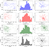 |
Fig. B.1. Each of the four clusters in the sample with a logarithmic scatter δη > 0.8 dex. Left: PPS. Central: LOS velocity distribution. Right: Projected positions with respect to the cluster centre. |
Appendix C: Stacked projected phase spaces in bins of 
In Fig. C.1 we plot the PPS of the five stacked clusters obtained by collecting member galaxies in bins of SZ masses, for T1 (top plots, blue points) and T2 (bottom plots, green points).
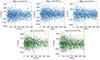 |
Fig. C.1. PPS parameters (radius, R, and radial velocity, v) for the SZ-stacked clusters. Top, blue points: T1. Bottom, green points: T2. The vertical dashed lines indicate the average r500 of all the clusters in each stacking. |
Appendix D: GTC cluster data
Here we report an extract of the member galaxies with measured spectroscopic redshifts for the three clusters observed with the OSIRIS spectrograph at the GTC. These three catalogues are organised as follow: first column corresponds to an ID label; the second and third columns indicate the right ascension and declination coordinates in J2000 epoch (RA and Dec); the fourth is the measured redshift and the last column is the errors on the redshift. The full catalogues are available upon request to the authors.
Extract of the galaxies with measured spectroscopic redshifts in the field of PSZ2G083.29-31.03.
Extract of the galaxies with measured spectroscopic redshifts in the field of PSZ2G113.91-37.01.
Extract of the galaxies with measured spectroscopic redshifts in the field of PSZ2G046.10+27.18.
Appendix E: Cluster members and velocity dispersion
In Fig. E.1 we show for each cluster the number of cluster members N200 that remains after the CLEAN procedure within R = rap, 200 (see also Fig. 4 of Sereno et al. 2025), plotted against the aperture velocity dispersion σap, 200. It is worth noticing that the majority of clusters have more than 100 members, making the CHEX-MATE catalogue a very good sample for kinematical analyses of galaxy cluster.
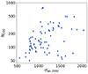 |
Fig. E.1. Number of members within R = rap, 200 after the application of the CLEAN algorithm, in relation to the aperture velocity dispersion σap, 200. |
All Tables
Results for the parameters of the linear fits of the relations discussed in this paper.
Constraints on the free parameters from the kinematic analysis with MG-MAMPOSST, shown for the combination of mass and number density model that provides the best BIC.
Extract of the galaxies with measured spectroscopic redshifts in the field of PSZ2G083.29-31.03.
Extract of the galaxies with measured spectroscopic redshifts in the field of PSZ2G113.91-37.01.
Extract of the galaxies with measured spectroscopic redshifts in the field of PSZ2G046.10+27.18.
All Figures
|
Fig. 1. Cluster redshift and |
| In the text | |
|
Fig. 2. Mass profile (top) and radial velocity anisotropy profile (bottom) of the cluster PSZ2 G067.17+67.46, as obtained via the MG-MAMPOSST analysis with Ngal = 299 galaxies and adopting a NFW model and a gT model, respectively. In both plots, darker and lighter shaded regions refer to 68% and 95% CLs, respectively. The vertical dashed line in the top panel identifies the best fit for r200 = 2.19 Mpc. |
| In the text | |
|
Fig. 3. Scatter plot of Log M200, inferred from the kinematic analysis with MG-MAMPOSST (vertical axis), and Log Mσ, 200c obtained by Sereno et al. (2025, horizontal axis). The error bars represent the 68% CL, and the dashed black line the bisector. Darker points highlight those clusters for which Log (M200M/Mσ, 200c) > 0.3. |
| In the text | |
|
Fig. 4. Logarithm of the aperture velocity dispersion within R = r200, σap, 200 compared to the logarithm of M200M estimated from MG-MAMPOSST. The bars refer to 68% uncertainties. The blue line indicates the best-fit linear model of Eq. (9) when z = 0.2. The solid black line identifies the σ ∝ M3 relation. |
| In the text | |
|
Fig. 5. Scatter plot of M500 inferred from the SZ effect by Planck (on the vertical axis) and from the kinematic analysis with MG-MAMPOSST (horizontal axis). The error bars represent the 68% CL, and the red points show those clusters for which the logarithmic difference (δη) is larger than 0.8 dex. Dark green points highlight clusters belonging to T2. The purple line is the ODR fit that considers all the clusters, while the blue one is the linear fit done by discarding the four outliers. The best-fit (with the outliers removed) linear models for T1 and T2 are shown separately with the dashed red and dark green lines, respectively. |
| In the text | |
|
Fig. 6. LOS velocity distribution for the system PSZ2G218.81+35.51, made of two separate clusters, as mentioned in Sereno et al. (2025). |
| In the text | |
|
Fig. 7.
|
| In the text | |
|
Fig. 8. Concentration–mass relation for the CHEX-MATE sample. The error bars indicate 68% uncertainties in the parameters; we highlight in light blue the clusters with |
| In the text | |
|
Fig. 9.
|
| In the text | |
|
Fig. 10. Fraction of galaxies in substructures, fsub, as a function of the logarithm of the Anderson-Darling coefficient, A2. The darker stars indicate the clusters for which Log (M200M/Mσ, 200c) > 0.3. |
| In the text | |
|
Fig. 11. Radial velocity anisotropy profiles for stacked clusters, where the stacking is in velocity dispersion. The bands show the 68% and 95% regions, and the black curve is the median profile. Top: z < 0.2. Bottom: z > 0.2. The bottom-right plot shows the value of β(r = r200) with 68% error bars (blue and red for z < 0.2 and z > 0.2, respectively). In all plots, the vertical dashed lines indicate the average rap, 200 in the corresponding velocity dispersion bin. |
| In the text | |
|
Fig. 12. Radial velocity anisotropy profiles for the stacked clusters, where the stacking is in bins of |
| In the text | |
|
Fig. B.1. Each of the four clusters in the sample with a logarithmic scatter δη > 0.8 dex. Left: PPS. Central: LOS velocity distribution. Right: Projected positions with respect to the cluster centre. |
| In the text | |
|
Fig. C.1. PPS parameters (radius, R, and radial velocity, v) for the SZ-stacked clusters. Top, blue points: T1. Bottom, green points: T2. The vertical dashed lines indicate the average r500 of all the clusters in each stacking. |
| In the text | |
|
Fig. E.1. Number of members within R = rap, 200 after the application of the CLEAN algorithm, in relation to the aperture velocity dispersion σap, 200. |
| In the text | |
Current usage metrics show cumulative count of Article Views (full-text article views including HTML views, PDF and ePub downloads, according to the available data) and Abstracts Views on Vision4Press platform.
Data correspond to usage on the plateform after 2015. The current usage metrics is available 48-96 hours after online publication and is updated daily on week days.
Initial download of the metrics may take a while.