| Issue |
A&A
Volume 699, July 2025
|
|
|---|---|---|
| Article Number | A214 | |
| Number of page(s) | 28 | |
| Section | Astrophysical processes | |
| DOI | https://doi.org/10.1051/0004-6361/202554838 | |
| Published online | 14 July 2025 | |
Euclid: Early Release Observations – The surface brightness and colour profiles of the far outskirts of galaxies in the Perseus cluster⋆
1
Université Paris-Saclay, Université Paris Cité, CEA, CNRS, AIM, 91191 Gif-sur-Yvette, France
2
Department of Physics, Université de Montréal, 2900 Edouard Montpetit Blvd, Montréal, Québec H3T 1J4, Canada
3
Ciela Institute – Montréal Institute for Astrophysical Data Analysis and Machine Learning, Montréal, Québec, Canada
4
Mila – Québec Artificial Intelligence Institute, Montréal, Québec, Canada
5
INAF-Osservatorio di Astrofisica e Scienza dello Spazio di Bologna, Via Piero Gobetti 93/3, 40129 Bologna, Italy
6
Univ. Lille, CNRS, Centrale Lille, UMR 9189 CRIStAL, 59000 Lille, France
7
Université Paris-Saclay, CNRS, Institut d’astrophysique spatiale, 91405 Orsay, France
8
Max Planck Institute for Extraterrestrial Physics, Giessenbachstr. 1, 85748 Garching, Germany
9
School of Physics and Astronomy, University of Nottingham, University Park, Nottingham NG7 2RD, UK
10
Universität Innsbruck, Institut für Astro- und Teilchenphysik, Technikerstr. 25/8, 6020 Innsbruck, Austria
11
Max-Planck-Institut für Astronomie, Königstuhl 17, 69117 Heidelberg, Germany
12
Laboratoire d’Astrophysique de Bordeaux, CNRS and Université de Bordeaux, Allée Geoffroy St. Hilaire, 33165 Pessac, France
13
Institut universitaire de France (IUF), 1 rue Descartes, 75231 PARIS CEDEX 05, France
14
Departamento de Física Teórica, Atómica y Óptica, Universidad de Valladolid, 47011 Valladolid, Spain
15
Instituto de Astrofísica e Ciências do Espaço, Faculdade de Ciências, Universidade de Lisboa, Tapada da Ajuda, 1349-018 Lisboa, Portugal
16
INAF-Osservatorio Astronomico di Capodimonte, Via Moiariello 16, 80131 Napoli, Italy
17
Centre de Recherche Astrophysique de Lyon, UMR5574, CNRS, Université Claude Bernard Lyon 1, ENS de Lyon, 69230 Saint-Genis-Laval, France
18
Universitäts-Sternwarte München, Fakultät für Physik, Ludwig-Maximilians-Universität München, Scheinerstrasse 1, 81679 München, Germany
19
Sterrenkundig Observatorium, Universiteit Gent, Krijgslaan 281 S9, 9000 Gent, Belgium
20
Université de Strasbourg, CNRS, Observatoire astronomique de Strasbourg, UMR 7550, 67000 Strasbourg, France
21
Instituto de Astrofísica de Canarias, Vía Láctea, 38205 La Laguna, Tenerife, Spain
22
Universidad de La Laguna, Departamento de Astrofísica, 38206 La Laguna, Tenerife, Spain
23
School of Mathematics and Physics, University of Surrey, Guildford, Surrey GU2 7XH, UK
24
INAF-Osservatorio Astronomico di Brera, Via Brera 28, 20122 Milano, Italy
25
IFPU, Institute for Fundamental Physics of the Universe, Via Beirut 2, 34151 Trieste, Italy
26
INAF-Osservatorio Astronomico di Trieste, Via G. B. Tiepolo 11, 34143 Trieste, Italy
27
INFN, Sezione di Trieste, Via Valerio 2, 34127 Trieste TS, Italy
28
SISSA, International School for Advanced Studies, Via Bonomea 265, 34136 Trieste TS, Italy
29
INAF-Osservatorio Astronomico di Padova, Via dell’Osservatorio 5, 35122 Padova, Italy
30
Dipartimento di Fisica, Università di Genova, Via Dodecaneso 33, 16146 Genova, Italy
31
INFN-Sezione di Genova, Via Dodecaneso 33, 16146 Genova, Italy
32
Department of Physics “E. Pancini”, University Federico II, Via Cinthia 6, 80126 Napoli, Italy
33
Instituto de Astrofísica e Ciências do Espaço, Universidade do Porto, CAUP, Rua das Estrelas, PT4150-762 Porto, Portugal
34
Faculdade de Ciências da Universidade do Porto, Rua do Campo de Alegre, 4150-007 Porto, Portugal
35
INAF-Osservatorio Astrofisico di Torino, Via Osservatorio 20, 10025 Pino Torinese (TO), Italy
36
INAF-IASF Milano, Via Alfonso Corti 12, 20133 Milano, Italy
37
INAF-Osservatorio Astronomico di Roma, Via Frascati 33, 00078 Monteporzio Catone, Italy
38
INFN section of Naples, Via Cinthia 6, 80126 Napoli, Italy
39
Dipartimento di Fisica e Astronomia “Augusto Righi” – Alma Mater Studiorum Università di Bologna, Viale Berti Pichat 6/2, 40127 Bologna, Italy
40
Institute for Astronomy, University of Edinburgh, Royal Observatory, Blackford Hill, Edinburgh EH9 3HJ, UK
41
Jodrell Bank Centre for Astrophysics, Department of Physics and Astronomy, University of Manchester, Oxford Road Manchester M13 9PL, UK
42
European Space Agency/ESRIN, Largo Galileo Galilei 1, 00044 Frascati, Roma, Italy
43
ESAC/ESA, Camino Bajo del Castillo, s/n., Urb. Villafranca del Castillo, 28692 Villanueva de la Cañada, Madrid, Spain
44
Université Claude Bernard Lyon 1, CNRS/IN2P3, IP2I Lyon, UMR 5822, Villeurbanne F-69100, France
45
Institut de Ciències del Cosmos (ICCUB), Universitat de Barcelona (IEEC-UB), Martí i Franquès 1, 08028 Barcelona, Spain
46
Institució Catalana de Recerca i Estudis Avançats (ICREA), Passeig de Lluís Companys 23, 08010 Barcelona, Spain
47
UCB Lyon 1, CNRS/IN2P3, IUF, IP2I Lyon, 4 rue Enrico Fermi, 69622 Villeurbanne, France
48
Mullard Space Science Laboratory, University College London, Holmbury St Mary, Dorking, Surrey RH5 6NT, UK
49
INAF-Istituto di Astrofisica e Planetologia Spaziali, Via del Fosso del Cavaliere, 100, 00100 Roma, Italy
50
Space Science Data Center, Italian Space Agency, Via del Politecnico snc, 00133 Roma, Italy
51
School of Physics, HH Wills Physics Laboratory, University of Bristol, Tyndall Avenue, Bristol BS8 1TL, UK
52
INFN-Sezione di Bologna, Viale Berti Pichat 6/2, 40127 Bologna, Italy
53
Institute of Theoretical Astrophysics, University of Oslo, P.O. Box 1029 Blindern 0315 Oslo, Norway
54
Jet Propulsion Laboratory, California Institute of Technology, 4800 Oak Grove Drive, Pasadena, CA 91109, USA
55
Felix Hormuth Engineering, Goethestr. 17, 69181 Leimen, Germany
56
Technical University of Denmark, Elektrovej 327, 2800 Kgs. Lyngby, Denmark
57
Cosmic Dawn Center (DAWN), DTU Space, Elektrovej 327. 2800 Kgs. Lyngby., Denmark
58
NASA Goddard Space Flight Center, Greenbelt, MD 20771, USA
59
Department of Physics and Helsinki Institute of Physics, Gustaf Hällströmin katu 2, 00014 University of Helsinki, Finland
60
Aix-Marseille Université, CNRS/IN2P3, CPPM, Marseille, France
61
Department of Physics, P.O. Box 64 00014 University of Helsinki, Finland
62
Helsinki Institute of Physics, Gustaf Hällströmin katu 2, University of Helsinki, Helsinki, Finland
63
Laboratoire d’etude de l’Univers et des phenomenes eXtremes, Observatoire de Paris, Université PSL, Sorbonne Université, CNRS, 92190 Meudon, France
64
SKA Observatory, Jodrell Bank, Lower Withington, Macclesfield, Cheshire SK11 9FT, UK
65
Dipartimento di Fisica “Aldo Pontremoli”, Università degli Studi di Milano, Via Celoria 16, 20133 Milano, Italy
66
INFN-Sezione di Milano, Via Celoria 16, 20133 Milano, Italy
67
University of Applied Sciences and Arts of Northwestern Switzerland, School of Computer Science, 5210 Windisch, Switzerland
68
Universität Bonn, Argelander-Institut für Astronomie, Auf dem Hügel 71, 53121 Bonn, Germany
69
INFN-Sezione di Roma, Piazzale Aldo Moro, 2 – c/o Dipartimento di Fisica, Edificio G. Marconi, 00185 Roma, Italy
70
Institut d’Astrophysique de Paris, 98bis Boulevard Arago, 75014 Paris, France
71
Institut d’Astrophysique de Paris, UMR 7095, CNRS, and Sorbonne Université, 98 bis boulevard Arago, 75014 Paris, France
72
Institute of Physics, Laboratory of Astrophysics, Ecole Polytechnique Fédérale de Lausanne (EPFL), Observatoire de Sauverny, 1290 Versoix, Switzerland
73
Dipartimento di Fisica e Astronomia “Augusto Righi” – Alma Mater Studiorum Università di Bologna, Via Piero Gobetti 93/2, 40129 Bologna, Italy
74
European Space Agency/ESTEC, Keplerlaan 1, 2201 AZ Noordwijk, The Netherlands
75
Institut de Física d’Altes Energies (IFAE), The Barcelona Institute of Science and Technology, Campus UAB, 08193 Bellaterra (Barcelona), Spain
76
DARK, Niels Bohr Institute, University of Copenhagen, Jagtvej 155, 2200 Copenhagen, Denmark
77
Waterloo Centre for Astrophysics, University of Waterloo, Waterloo, Ontario N2L 3G1, Canada
78
Department of Physics and Astronomy, University of Waterloo, Waterloo, Ontario N2L 3G1, Canada
79
Perimeter Institute for Theoretical Physics, Waterloo, Ontario N2L 2Y5, Canada
80
Centre National d’Etudes Spatiales – Centre spatial de Toulouse, 18 avenue Edouard Belin, 31401 Toulouse Cedex 9, France
81
Institute of Space Science, Str. Atomistilor, nr. 409 Măgurele, Ilfov 077125, Romania
82
Dipartimento di Fisica e Astronomia “G. Galilei”, Università di Padova, Via Marzolo 8, 35131 Padova, Italy
83
INFN-Padova, Via Marzolo 8, 35131 Padova, Italy
84
Institut d’Estudis Espacials de Catalunya (IEEC), Edifici RDIT, Campus UPC, 08860 Castelldefels, Barcelona, Spain
85
Satlantis, University Science Park, Sede Bld 48940, Leioa-Bilbao, Spain
86
Institute of Space Sciences (ICE, CSIC), Campus UAB, Carrer de Can Magrans, s/n, 08193 Barcelona, Spain
87
Departamento de Física, Faculdade de Ciências, Universidade de Lisboa, Edifício C8, Campo Grande, PT1749-016 Lisboa, Portugal
88
Universidad Politécnica de Cartagena, Departamento de Electrónica y Tecnología de Computadoras, Plaza del Hospital 1, 30202 Cartagena, Spain
89
Port d’Informació Científica, Campus UAB, C. Albareda s/n, 08193 Bellaterra (Barcelona), Spain
90
Centro de Investigaciones Energéticas, Medioambientales y Tecnológicas (CIEMAT), Avenida Complutense 40, 28040 Madrid, Spain
91
Institut de Recherche en Astrophysique et Planétologie (IRAP), Université de Toulouse, CNRS, UPS, CNES, 14 Av. Edouard Belin, 31400 Toulouse, France
92
INFN-Bologna, Via Irnerio 46, 40126 Bologna, Italy
93
Infrared Processing and Analysis Center, California Institute of Technology, Pasadena, CA 91125, USA
94
INAF, Istituto di Radioastronomia, Via Piero Gobetti 101, 40129 Bologna, Italy
95
ICL, Junia, Université Catholique de Lille, LITL, 59000 Lille, France
⋆⋆ Corresponding author: maelie.mondelin@cea.fr
Received:
28
March
2025
Accepted:
6
May
2025
The Perseus field captured by Euclid as part of its Early Release Observations provides a unique opportunity to study cluster environment ranging from outskirts to dense regions. Leveraging unprecedented optical and near-infrared depths, we investigate the stellar structure of massive disc galaxies in this field. This study focuses on outer disc profiles, including simple exponential (Type I), down-bending break (Type II) and up-bending break (Type III) profiles, and their associated colour gradients, to trace late assembly processes across various environments. Type II profiles, though relatively rare in high dense environments, appear stabilised by internal mechanisms like bars and resonances, even within dense cluster cores. Simulations suggest that in dense environments, Type II profiles tend to evolve into Type I profiles over time. Type III profiles often exhibit small colour gradients beyond the break, hinting at older stellar populations, potentially due to radial migration or accretion events. We analyse correlations between galaxy mass, morphology, and profile types. Mass distributions show weak trends of decreasing mass from the centre to the outskirts of the Perseus cluster. Type III profiles become more prevalent, while Type I profiles decrease in lower-mass galaxies with cluster centric distance. Type I profiles dominate in spiral galaxies, while Type III profiles are more common in S0 galaxies. Type II profiles are consistently observed across all morphological types. While the limited sample size restricts statistical power, our findings shed light on the mechanisms shaping galaxy profiles in cluster environments. Future work should extend observations to the cluster outskirts to enhance statistical significance and explore looser environments. Additionally, 3D velocity maps are needed to achieve a non-projected view of galaxy positions, offering deeper insights into spatial distribution and dynamics.
Key words: Galaxy: disk / galaxies: evolution / galaxies: interactions / galaxies: clusters: individual: Perseus
© The Authors 2025
 Open Access article, published by EDP Sciences, under the terms of the Creative Commons Attribution License (https://creativecommons.org/licenses/by/4.0), which permits unrestricted use, distribution, and reproduction in any medium, provided the original work is properly cited.
This article is published in open access under the Subscribe to Open model. Subscribe to A&A to support open access publication.
1. Introduction
The study of the radial surface brightness distribution of galaxies enables decoding intricate patterns of light and the variations in brightness across different regions of galaxies, providing in turn crucial insights into their structure, formation, and evolution. By analysing these distributions, one can infer the presence of various components such as bulges, discs, and bars, and gain a deeper understanding of the underlying physical processes (de Vaucouleurs 1948; Freeman 1970; Sérsic 1963). de Vaucouleurs (1948) specifically describes galaxy discs as having declining exponential profiles. However, later observational results (van der Kruit 1979) have shown that these simple exponential profiles do not necessarily hold for some galaxies beyond a certain distance from the core. The development of deeper surveys, beyond a surface brightness of 25 mag arcsec−2, has revealed that disc profiles can be classified into three categories (Pohlen & Trujillo 2006; Erwin et al. 2008): Type I corresponds to the traditional decreasing exponential profile down to the twenty-fifth isophote or even beyond; Type II galaxies show a truncation and can be fitted by down-bending double exponentials; and Type III are up-bending break profiles, also known as up-bending double exponentials.
Studies on several hundreds of galaxies (Erwin et al. 2005, 2008) have revealed that down- and up-bending breaks occur near a surface brightness of 25 mag arcsec−2 in the visible spectrum, and are also present in the infrared profiles of galaxies (Muñoz-Mateos et al. 2013). It is important to clarify the terminology used in this context: some authors, such as Buitrago & Trujillo (2024), refer to the outermost break in a galaxy’s surface brightness or mass profile (which coincides with the disc termination) as down-bending breaks or galaxy edges. However, in this paper, we use the term ‘down-bending break’ specifically to describe a bending in the galaxy surface brightness profile, regardless of its location relative to the disc edge.
Additionally, Gutiérrez et al. (2011) showed that the proportion of each Type I in the optical R-band varies according to the morphology of galaxies. More than 80% of late-type spiral galaxies have Type II profiles. The fraction of these types changes gradually with the evolution of galaxies. For early-type galaxies, including lenticulars and early-type spirals, Type III profiles dominate at 50%, with the remaining galaxies having profiles split between Type I and Type II.
Given these observations, the origin of down- and up-bending disc breaks has been questioned since their discovery. Down-bending disc breaks, meaning Type II profiles, can be explained by two main scenarios. The first scenario encompasses several explanations related to dynamical phenomena. The role of bars and their outer Lindblad resonance has been questioned. Elmegreen & Hunter (2006) propose that the outer Lindblad resonance of bars may cause angular momentum redistribution, contributing to the formation of down-bending breaks.
Observations show that the link between the break radius and outer rings or outer lenses is undeniable, especially for early-type spirals or lenticulars (Laine et al. 2016). The formation of clumps at higher redshifts could also explain these down-bending disc breaks (Xu & Yu 2024). The second scenario primarily applies to young spiral galaxies and proposes that down-bending disc breaks occur because the distribution of cold gas in the discs falls below a critical density threshold for star formation beyond the truncation radius (Kennicutt 1989; Schaye 2004; Elmegreen & Hunter 2006). The phenomenon of stellar migration also reveals that stars formed in the inner disc can migrate to the outermost regions of the disc, populating them with old red stars (Sellwood & Binney 2002; Debattista et al. 2006; Roškar et al. 2008a). These down-bending disc breaks in the profiles are also observed in simulations (Bournaud et al. 2007; Elmegreen & Struck 2013; Struck & Elmegreen 2016).
Regarding Type III profiles, meaning up-bending break profiles, the hypotheses are related to internal disc phenomena as well as external environmental factors. Observations of young star emission in the outer regions of discs suggest ongoing star formation, indicating the presence of cold gas in these regions (Gil de Paz et al. 2005; Thilker et al. 2005; Tsvetkov et al. 2024). In contrast, in the context of hierarchical evolution, spiral galaxies undergo mergers and interactions with neighbouring galaxies over their evolutionary history. This can lead to an excess of red stars in the outer regions. Simulations and observations, particularly in our own galaxy (Toomre & Toomre 1972), show that gravitational interactions, major and minor mergers can lead to the formation of tidal tails, shell, loops and disc perturbations. For major mergers, works such as Borlaff et al. (2014) indicate that an up-bending break profile could be produced after an accretion event, especially with a break at higher surface brightness. In many cases, the minor mergers have also an important role in the evolution of disc galaxies and result in episodes of dwarf galaxies accretion within a spiral galaxy. These satellites are gradually assimilated into the galactic halo and eventually into the outer disc (Helmi et al. 1999, 2018; Belokurov et al. 2018; Koppelman et al. 2019; Myeong et al. 2019; Horta et al. 2021). This process also disrupts the dynamical equilibrium of the disc, kinetically heating the disc stars and moving them to outer disc orbits, and even into the stellar halo (Nissen & Schuster 2010; Haywood et al. 2018). Therefore, stars originating from both the remnants of satellite galaxies and the initial disc stars could be responsible for these up-bending disc breaks (Younger et al. 2007; Eliche-Moral et al. 2011), in other words, an excess of light beyond a certain radius. Gaia observations of our Galaxy also confirm the presence of two disc components in the Galaxy, thin and thick, with different scale lengths.
The role of the environment is therefore debated for Type III galaxies and for Type II, as the phenomenon of disc warping could be a source of truncation (Roškar et al. 2008b; Sánchez-Blázquez et al. 2009). Early studies on clusters reached ambiguous conclusions. A study of S0 galaxies in the Virgo cluster (Erwin et al. 2012) showed that the cluster galaxies can be compared to field galaxies. First, the proportions of up-bending disc breaks within the cluster and outside are equal. Additionally, Type II down-bending break profiles are not present in this cluster. Thus, as galaxies approach the cluster, due to various effects such as ram-pressure stripping, strangulation and harassment, they may lose their truncation, becoming either Type I galaxies or, in some cases, initially Type I galaxies becoming up-bending break. However, this result is questioned by Laine et al. (2016) which suggests that Type II profiles are not absent from the Virgo cluster because of three down-bending break profiles on 24 Virgo cluster members in the sample. In addition, the Coma cluster as studied for instance by Head et al. (2015) challenges these previous results on S0 galaxies in clusters. According to their results, disc down-bending breaks are present in the cluster up to the core. This study also highlighted the role of bars in stabilising down- and up-bending disc breaks. Overall, the above-mentioned findings on two clusters, Coma and Virgo, reach different conclusions relative to the impact of environmental factors on disc profiles. Recent findings have found more perturbed galaxies in Type II and III than in Type I (Sánchez-Alarcón et al. 2023). This supports the formation scenario in which Type III discs are formed via interactions such as major mergers, and Type II discs stem from a star formation threshold (Laine et al. 2016; Watkins et al. 2019; Pranger et al. 2017). As of today, this question is consequently left unanswered but could be explored further by improving statistics, in the number of clusters observed, and the quality of observations.
The Perseus cluster, located at 72 Mpc from us, was previously covered by the Hubble Space Telescope at 30% sky coverage through multiple stacks. The new Euclid Release Observation – Perseus programme (Cuillandre et al. 2025a,b) now offers an unprecedented view of a 0.7 deg2 (1 Mpc2) field at Perseus cluster distance, providing a groundbreaking perspective of the cluster. The combination of the high resolution of the visible imager (Euclid Collaboration: Cropper et al. 2025; Euclid Collaboration: Mellier et al. 2025), called VIS, and the infrared information from the near-infrared spectrometer and photometer (NISP) is unprecedented over such a large field. This wide field allows for a comprehensive and controlled analysis with good statistical reliability. Note that observing down- and up-bending disc breaks in the cores of clusters has historically been challenging due to the dominance of intracluster light (Kluge et al. 2025).
Thanks to its remarkable depth and capacity to capture diffuse stellar halos (Cuillandre et al. 2025a), Euclid (Euclid Collaboration: Mellier et al. 2025) reveals the outermost regions of galaxies, specifically areas beyond the location of the break for Type II or III. The measured luminosity profiles extend beyond 28 mag arcsec−2 for most galaxies in the cluster in both the optical and the near-infrared (NIR), enabling us to study the various components of the disc and the fainter parts of the galaxy in great detail. Additionally, the unique capabilities of the NISP instrument (Euclid Collaboration: Jahnke et al. 2025) across three photometric bands provide valuable near-infrared information, which allows us to examine the distribution of older stars within the discs. This combination of deep field optical and near-infrared imaging offers a comprehensive view of both the young and old stellar populations, contributing significantly to our understanding of galaxy formation and evolution in cluster environments.
Within the framework of these Euclid Early Release Observations (2024), we study the disc profiles of galaxies observed within the Perseus cluster, focusing mainly on S0 galaxies but also including some early-type spirals. This paper is organised as follows. In Sect. 2, we will describe precise photometric extraction, followed by fitting different models to detect morphological characteristics. Subsequently, in Sect. 3, we will study the characteristics of down- and up-bending disc breaks, such as surface brightness and break radius, as well as the influence of mass and colour. In Sect. 5, we will discuss the implications of our observations and conclude on possible processes of galaxy evolution in the Perseus cluster.
2. Method
2.1. Data and sample selection
Galaxies in the Euclid Early Release Observations (ERO) Perseus cluster were identified in Cuillandre et al. (2025b) and Marleau et al. (2025). The brightest galaxies were assigned to the cluster based primarily on available spectroscopic redshifts or alternatively photometric redshifts. For fainter or smaller galaxies, visual inspection of the images was also used to confirm their cluster membership. As described in Cuillandre et al. (2025b), 136 bright galaxies are members of the cluster within the 0.7 deg2 ERO Perseus field. Figure 1 shows the positions of the disc and elliptical galaxies overlaid on the low surface brightness (LSB) image of the cluster in IE. Note that isophotal models for NGC 1275 (including the surrounding intracluster light) and NGC 1272 were subtracted, as well as the interstellar medium (using the Wise 12 μm map), as detailed in Kluge et al. (2025). The influence of ICL on the classification and surface brightness profiles of these galaxies is explored in detail in Appendix A. This appendix shows how important it is to ensure that down- or up-bending disc breaks are not overlooked. We show the scaling relations in Fig. 2 – which illustrates key structural parameters (Sérsic index n, effective radius Re, central surface brightness μ0, and mean effective surface brightness ⟨μe⟩) for disc and elliptical galaxies extracted from Cuillandre et al. (2025b). We identify 102 out of 136 galaxies as disc systems. We show the distributions of disc galaxies in blue, while red points represent ellipticals, with normalised histograms offering a comparative view of each type’s parameter distributions. Details of this classification by morphology are given in Sect. 2.5.
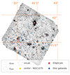 |
Fig. 1. IE image of the Perseus field of view after subtraction of the intra-cluster light (ICL): blue dots indicate the position of each disc galaxy, red dots show the position of ellipticals. Orange lines shows the right ascension and the declination of IE image. In the background, the method of identification for each galaxy is displayed, with visual markers distinguishing galaxies classified by photometric redshifts (zphot, square symbols) and spectroscopic redshifts (zspec, circular symbols). The yellow dot highlights the location of the cluster centre (NGC 1275). |
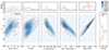 |
Fig. 2. Scaling relations between the Sérsic index n, the effective radius Re, the central surface brightness μ0, mean effective surface brightness within Re, ⟨μe⟩, the mass log10(M*/M⊙) and the total magnitude IE of galaxies measured using AutoProf/AstroPhot. The blue distribution shows the probability density function for the 102 cluster member bright disc galaxies while red dots are for cluster member bright ellipticals. The surface brightness is given in mag arcsec−2. The panels on the top and side provide the normalised histograms of the parameters for discs (in blue) and for ellipticals (in red). |
2.2. Gravitational interactions in the sample
After selecting the large galaxies in the Perseus cluster, galaxies which are not considered as dwarfs in Cuillandre et al. (2025b), we inspect each one for signs of interaction in order to place them in the overall context of the cluster. The Perseus cluster, often perceived as a graveyard of evolved galaxies, is in fact a complex and dynamic environment where gravitational interactions, ram pressure and tidal forces play a crucial role in galaxy evolution. This framework enables us to better interpret the perturbations observed in the outer regions of these discy galaxies. Multi-wavelength studies, including X–ray and radio observations (van Weeren et al. 2024), have revealed numerous signs of past and present activity in this cluster. For example, the X-ray centre of the cluster (HyeongHan et al. 2025) is off-centred with respect to the gravitational centre of mass, an observation corroborated by the mis-centreing of the ICL and globular clusters (Kluge et al. 2025). This context highlights the diversity of environmental interactions affecting galaxies in clusters, particularly in the Perseus cluster.
Here, we observe at high resolution in IE images that approximately 20% exhibit significant signs of disturbances in their outer isophotes. When considering possible minor mergers/satellite galaxies, this rate rises to 50%. It should be noted that these rates of disturbed galaxies are likely even higher as they are immersed in a sea of dwarf galaxies, the ICL and the cluster’s gravitational potential well.
This general framework lays the foundations for our photometric analysis, where we seek to characterise the perturbations of galaxy outer discs. Figure 3 illustrates the diversity of interactions revealed in IE band LSB images, with processes such as mergers and dynamic pressure clearly influencing morphologies. Note that in the red-green-blue (RGB) image – Fig. 1 in Cuillandre et al. (2025b) – streams and various outer isophotes marked by rather orange hues can also be observed. These features are highlighted using the HE band image, which reveals diffuse and extended structures, often associated with stellar remnants from interacting galaxies. These red hues indicate older stellar populations, typical of the outer regions of post-interaction galaxies, where newly formed stars are absent, leaving a halo reddened by stellar ageing. Additionally, in galaxies undergoing ram pressure stripping, blue zones of star formation are visible in regions of the cluster within the gas stripped from the galaxy. The pockets of star-forming activity at the faintest levels outside the galaxies are studied in George et al. (in prep.).
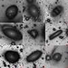 |
Fig. 3. Examples of different types of interactions observed in the Perseus cluster. Each panel shows a LSB IE image with high contrast of a galactic interaction within the cluster. A red line in the bottom-right corner representing a scale of 10″ is provided at the bottom of each panel. Top left: NGC 1268 – a galaxy with a smooth, elongated shape, likely experiencing a close encounter with a neighbouring galaxy, causing mild distortion in its outer regions. Top centre: NGC 1282 – an interacting galaxy with a faint halo, possibly stripped due to gravitational forces from nearby massive galaxies. Top right: GALEXASC J031939.68+413105.6 – a disrupted galaxy showing two tidal rings, suggesting a recent interaction or minor merger with another galaxy. Middle left: PGC 012221 – a galaxy with a clear spiral structure that appears distorted, possibly due to tidal forces. Middle centre: PGC 012358 – a major merger with an asymmetrical shape and tidal tails, showing evidence of material being pulled away. Middle right: PGC 012520 – an elongated galaxy with an asymmetric stretched halo, suggesting ongoing gravitational interactions or stripping by the cluster’s dense environment. Bottom left/centre: MCG+07-07-070 and UGC 02665 – galaxies possibly affected by ram pressure stripping due to their motion through the intracluster medium. MCG+07-07-070 shows an asymmetric diffuse halo extending towards the lower right, while UGC 02665 displays an umbrella-like morphology, both consistent with ram-pressure stripping (George et al. in prep.). Bottom right: WISEA J032020.96+41225.4 – a galaxy interacting with a larger galaxy, showing faint tidal features, which may indicate gravitational influence from a nearby massive galaxy. |
We also note that cosmological simulations, such as those in Martig et al. (2012) and Kraljic et al. (2012), help improve our understanding of the detection of tidal debris and interaction remnants at different depths. For example, Mancillas et al. (2019) shows that at a limiting surface brightness of 29 mag arcsec−2, only a portion of the tidal debris detectable at 33 mag arcsec−2 becomes visible. Although these simulations often focus on a limited sample, they consistently reveal the persistence of tidal features and debris from different interaction epochs. This provides a realistic benchmark for our detection limits in ERO images, which reach down to 30 mag arcsec−2 in the outer regions and around 27 mag arcsec−2 in the cluster centre, where the ICL strongly dominates the galaxy’s flux (Kluge et al. 2025).
With this big picture of the dynamical state of the Perseus cluster, we can now detail the method for photometrically extracting the luminosity profiles of the selected disc galaxies, focusing on quantifying the deformations and characteristics of the outer isophotes to better pinpoint the effects of the environment on these galactic structures.
2.3. Extraction of surface brightness profiles
In this study, we adopt the photometric extraction method detailed in Cuillandre et al. (2025b) in order to extract the profiles. The performance of the VIS and NISP cameras, as well the LSB processing of the ERO pipeline (Cuillandre et al. 2025a) have enabled unprecedented depth across this wide field. Additionally, the study of the ICL in the Perseus cluster (Kluge et al. 2025) facilitates the subtraction of this diffuse flux from the original images, allowing for more precise photometry of the galaxies’ outermost regions. The flux from the two central giant ellipticals, NGC 1275 and NGC 1272, is also subtracted from the IE images to limit their contributions to neighbouring galaxies, based on the residual maps developed in Kluge et al. (2025). Since the surface brightness of the ICL affects values around 27 mag arcsec−2, which is approximately 1 magnitude fainter than the range where profile breaks are typically observed (24–26 mag arcsec−2), we expected minimal impact on break detection. To confirm this, we compared galaxy profiles extracted from images with and without ICL subtraction and verified that the presence of ICL does not significantly affect the detection of breaks. We found that differences between the two cases are mainly notable for the most central galaxies. In these cases, the ICL subtraction step is crucial, as the galaxies are located very close to the extended envelopes of the central ellipticals and deeply embedded in the diffuse intracluster light. At larger distances, beyond the median cluster-centric distance of our sample, discrepancies between profiles extracted with and without ICL subtraction appear only at very faint surface brightness levels, after 26 mag arcsec−2, and do not affect the identification of profile breaks, which occur at larger surface brightness levels. A detailed comparison illustrating this effect is provided in Appendix A.
From there, square tiles centred on each galaxy are then extracted. The size of each tile is chosen according to the angular size of the galaxy: 1 k ×1 k pixel (i.e. 1 7 × 1
7 × 1 7), 2 k × 2 k pixel, (i.e 3
 3 × 3
3 × 3 3), or 4 k × 4 k pixel, (i.e. 6
 7 × 6
7 × 6 7) for the largest galaxies. After masking the bright stars and small galaxies near the main galaxies on each tile, the AutoProf tool (Stone et al. 2021) is used to extract the photometry of the individual galaxies. AutoProf is a pipeline that adjusts isophotes of varying semi-major axes around an isolated galaxy in an image to extract the galaxy’s surface brightness, ellipticity, and PA as a function of the semi-major axis. Note that in our context, isolated refers to galaxies sufficiently separated from neighbours such that masking nearby objects is adequate for reliable profile extraction. The tool also provides estimates of different biases and noise levels. Due to the extended point-spread function (PSF) of high purity as detailed in Cuillandre et al. (2025a), the deconvolution of the profiles by the PSF is not performed here. Note, however, that the Appendix B provides a rapid study of the influence of the extended PSF on model parameters. Instead, a simple point-source PSF model is used by AutoProf (Stone et al. 2021). However, for some disc galaxies whose envelopes overlap with those of their neighbours: the AstroPhot tool (Stone et al. 2023) is preferred for 15 out of the 102 disc galaxies in the sample, using 4 k × 4 k pixel tiles. AstroPhot is a tool designed to parameterise the surface brightness distribution of all galaxies and objects within an image. While AstroPhot could model all the galaxies within a 4 k × 4 k pixel tile, this approach requires significantly more computation time, compared to AutoProf – approximately five times longer – and the results are equivalent for isolated galaxies (Cuillandre et al. 2025b). We now detail in the two subsequent subsections how the profiles are obtained in practice from AutoProf and AstroPhot.
2.3.1. AutoProf photometric profiles
After extracting tiles corresponding to around 4 times the approximate apparent size of the galaxy, the next step is to mask the foreground stars that may contaminate the data. As detailed in Cuillandre et al. (2025b), the Perseus cluster is located close to the Galactic plane, and many bright stars overlap with the envelopes of the galaxies studied here. SExtractor (Bertin & Arnouts 1996), as indicated in Cuillandre et al. (2025b), is used to detect the stars, particularly by utilising the star-galaxy separation parameter, supplemented with visual inspection to validate or add stars. The pixels corresponding to stars within a radius of 800 IE pixels from the centre of the galaxy (80″), are masked using the separation parameter and a Fast Fourier Transform convolution of 10 × 10 pixel in order to increase the mask. The star masks are sometimes adjusted based on visual inspection, especially when stars extend over multiple pixels due to saturation. Then, a mask for neighbouring main galaxies is created: the average ellipticity is obtained from the axis ratio previously provided in the catalogue from Cuillandre et al. (2025b), and a masking ellipse with a semi-major axis of five times the effective radius is applied on each neighbouring galaxies at the centre. Additionally, background galaxies identified by SExtractor detections are also masked, with visual validation ensuring that only relevant galaxies are obscured, thereby minimising data contamination. As an illustration, Fig. 4 shows an example of masking for galaxy NGC 1270.
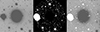 |
Fig. 4. Star masking process. Left: image of a 2 k × 2 k tile (i.e. 3 |


The masked image centred on a galaxy is then fed into the AutoProf run. Starting from a given position and using this image, a galaxy is fitted by the AutoProf pipeline. Several steps are involved in extracting the surface brightness profile of the galaxy. First, all bad pixels in the image are masked by the AutoProf procedure. A model of the background and then the PSF is derived to subtract a constant pedestal (the images being perfectly flat) starting from the given zero point, which is 30.132 for the ERO stacks. Note that the background subtraction is performed automatically, using the mode of the pixel flux distribution measured in the outermost regions of the image. This method, which applies a Gaussian-smoothing of the flux distribution to robustly estimate the sky background, is described in detail in Stone et al. (2021) and ensures minimal sensitivity to contamination from bright sources, which is crucial for accurate surface brightness measurements at faint levels. The centre of the image is also adjusted from an input centre. Using the masked image, elliptical isophotes are then initialised, fitted, and extracted to obtain the surface brightness profile. Radial isophotes are successively fitted until reaching the background level of the image. The pipeline outputs a 2D image showing the elliptical isophotes on the image, a 1D profile showing the surface brightness as a function of the semi-major axis of the isophotal ellipse, and a residual image. Figure 5 illustrates some steps of the AutoProf process for extracting the surface brightness profile of our galaxies.
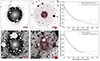 |
Fig. 5. Several steps of the AutoProf process for WISEA J031817.90+414031.0 for a IE (top) and a HE (bottom) images. Left: Initialisation of the first ellipse in cyan around the central galaxy. Middle: Final isophote fitting. Using red and cyan colours enhances the visualisation and counting of isophotes (Stone et al. 2021) Right: Extraction of the radial surface brightness profile. Note that cyan points are drawn each four isophotes. |
For the extraction of profiles in the YE, JE, and HE bands, a method of forced photometry with AutoProf is applied, using the IE profile as a reference. The principle remains the same as previously described, but it also leverages the solution from the IE image to extract the isophotes (Stone et al. 2021). Specifically, this approach fixes the centre, the position of the isophotes, as well as their orientation and ellipticity, based on the global isophote fit profile obtained from the IE AutoProf process. Since the NISP resolution is three times lower than that of VIS (pixel scale of IE band is equal to 0 1 compared to pixel scale of HE, YE, JE is 0
 3), this method benefits from the higher-resolution IE photometry for consistent isophote geometry.
2.3.2. AstroPhot photometric profiles
In the context of these observations of the core of the Perseus cluster, some galaxies overlap with their neighbours along the line of sight. In such peculiar cases, AutoProf produces a combined profile for two galaxies. Therefore, AstroPhot – which enables the comprehensive modelling of surface brightness profiles for all galaxies and objects within a large tile – is clearly more suitable for the 15 galaxies we identified as problematic for AutoProf. In these cases, 4 k × 4 k tiles around them are extracted. A masking process, also using SExtractor, is performed to mask the foreground stars in these tiles. Each galaxy in the field is then initialised with a spline galaxy model up to a radius limit determined by visual inspection, corresponding to the point where the noise seems to blend with the galaxy’s flux. The position angle (PA) and semi-major axis values are provided by the catalogue in Cuillandre et al. (2025b).
A spline radial light profile is interpolated for 50 points from the centre of the galaxy to the radius limit using a cubic spline interpolation of the stored brightness values. An initial model group, containing a model for each galaxy, is created. During the iterative fitting process, parameters such as the (PA), ellipticity, and flux distribution are adjusted for each galaxy while keeping the radii of the isophotes fixed. Similar to the approach described in the AutoProf analysis, the sky background is explicitly modelled. In this case, a flat sky model is adopted, in which the background is assumed to be constant across the tile. The background level is treated as a free parameter in the fit, enabling a robust estimation that accounts for any residual large-scale background and ensures reliable surface brightness measurements in complex and crowded environments. This iterative approach ensures an optimal fit for each galaxy in the crowded field, resulting in a 2D profile and a residual image. Note that the 1D profile is also derived directly by AstroPhot. Figure 6 illustrates the complete fitting process for these galaxies.
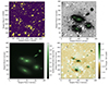 |
Fig. 6. Steps of the AstroPhot process for NGC 1260 and its neighbouring galaxies for a IE image. Top left: Detection of stars (in yellow) from the SExtractor segmentation map. Top right: Masking of stars on the 4 k × 4 k image centred on NGC 1260. Bottom left: Final fitting of galaxies provided by AstroPhot, colour coded by the surface brightness value. Bottom right: Final residual map. |
We note that the comparison of these photometric tools for isolated galaxies is discussed in Cuillandre et al. (2025b) and shows a good consistency between the two methods, with the extracted profiles superimposed. Over a dozen galaxies tested, we observed a difference of less than 1% on the radius measured at 25 mag arcsec−2 (called R25).
2.4. Classification by profile type
Each surface brightness profile extracted with AutoProf or Astrophot is then resampled with 300 points to obtain regularly spaced intervals in radius/semi-major axis along the surface brightness curve. This process involves applying a simple cubic interpolation and smoothing the curves. A careful visual inspection of the profiles was conducted to validate this step, ensuring the accuracy and consistency of the resampled data. Appendix C provides the complete set of profiles for both tools.
Moreover, before proceeding with the detailed analysis of the surface brightness profiles, the presence of a disc in each galaxy is first validated through a preliminary fitting process. According to Cuillandre et al. (2025b), 17 of the S0 galaxies from the initial catalogue have a Sérsic index n greater than 4, suggesting they are elliptical galaxies. However, after visual inspection of the galaxies and their profiles, this is attributed to two main phenomena: either the presence of a very bright and extended bulge or the presence of a bar (as suggested in Salo et al. (2015), which similarly distorts the profile. We confirm the presence of a disc component in all cases by employing a more sophisticated modelling approach than the simple Sérsic profile. This advanced modelling extends to a surface brightness of 25 mag arcsec−2, surpassing the initial rough estimate provided by the Sérsic profile. As Quilley et al. (in prep.) point out, the simple Sérsic approach proves inadequate for galaxies where both bulge and disc significantly contribute to the overall structure, such as in lenticular and early-type spiral galaxies. The existence of a residual disc is clearly evident in the surface brightness profile beyond a certain radius. This is characterised by a distinctive slope of one in the profile, typically emerging at surface brightnesses between 22 and24 mag arcsec−2.
This involves fitting a simple exponential disc + bulge decomposition, using data up to magnitude 25, as is traditionally done. The Sérsic index n is fixed to four during the fitting to accurately model the bulge, while the disc is modelled with an exponential function. This initial fit allows us to confirm the presence of a disc structure by ensuring that the disc component dominates the light profile beyond the bulge region. The results from this preliminary fitting provide the basic parameters and ensure the reliability of the subsequent analysis. This validation is particularly important for the 17 galaxies that initially had a high value of Sérsic indices for the fitting of a simple Sérsic model up to R25.
From the radial surface brightness profiles of the galaxies, our goal is to extract the physical parameters of the discs and notably determine the presence of a break, indicative of a Type II or Type III profile. Note that the classification takes into account only breaks that occur between 22 and 27 mag arcsec−2. The models adjust to account for the strongest break observed, although it’s true that double breaks probably exist. For instance, in a preliminary analysis of two late Type,III galaxies, a small down-bending break around 21–22 mag arcsec−2 was observed in their surface brightness profiles. However, these double breaks will not be discussed further in this paper.
Different models are fitted to the profile using the method employed in several studies (Erwin et al. 2005, 2008; Pohlen & Trujillo 2006; Muñoz-Mateos et al. 2013; Laine et al. 2016). A radial interval [rmin, rmax] within which these models are applied is defined for each galaxy through visual inspection. The minimum radius roughly corresponds to the inner radius of the galaxy where the bulge is located, beyond which the disc flux begins to dominate. The profile is fitted by a de Vaucouleurs profile before rmin and by a decreasing exponential in [rmin, rmax]. As suggested by several studies on bulge + disc decomposition of spiral galaxies (Allen et al. 2006; Kim et al. 2016; Gao et al. 2019; Quilley & de Lapparent 2023), allowing the Sérsic parameter to vary freely between one and four enables a better characterisation of the bulge. However, our study focuses primarily on the characterisation of the discs. Taking an intermediate Sérsic index like two risks blending the disc and the central bulge, which would contradict our intention to isolate the disc component. Therefore, a de Vaucouleurs profile seems sufficient as a first approximation, especially since it is particularly relevant for evolved galaxies with prominent bulges, such as those present in the Perseus cluster.
Additionally, the maximum radius corresponds to the point where the flux reaches the background noise level estimated by the AutoProf pipeline. While the photometric zero point is at 30.132 for IE and 30 for NISP (Cuillandre et al. 2025a), this background level is estimated around 29 mag arcsec−2, with punctual areas affected by structured galactic cirrus (well visible in this low galactic latitude field) limiting the detection at 28 mag arcsec−2.
From the intensity profile defined as
where ZP is the zero point and μ(r) is the surface brightness at radius r, we apply different model functions namely i) a simple exponential profile defined as
where I(r) is the intensity at radius r, I0 is the central intensity and hd is the scale length of the disc; and ii) a double exponential profile for Type II and Type III defined as
![$$ \begin{aligned} I(r) = S I_0 \exp \left({-\frac{r}{h_{\text{ d1}}}}\right) \left\{ 1 + \exp [\alpha (r - R_{\text{ break}})]\right\} ^p, \end{aligned} $$](/articles/aa/full_html/2025/07/aa54838-25/aa54838-25-eq13.gif)
with  and
and ![$ S^{-1} = 1 + \exp\left[-\alpha R_{\mathrm{break}}\left(\frac{1}{h_{\mathrm{d1}}} - \frac{1}{h_{\mathrm{d2}}}\right)\right] $](/articles/aa/full_html/2025/07/aa54838-25/aa54838-25-eq15.gif) ,
,
where I0 is the central intensity, hd1 is the inner scale length, hd2 is the outer scale length, Rbreak is the break radius, and α is a parameter that controls the sharpness of the transition between the two regions. This latter parameter is typically fixed to 0.5 (Erwin et al. 2008; Laine et al. 2016).
The values and uncertainties on the parameters are directly derived from the curve_fit Python fitting function. These models can now help us to characterise the surface brightness profiles of the galaxies and identify the presence of breaks indicative of Type II or Type III profiles.
For each model, the reduced chi-squared (χ2) value is calculated to determine the best fit. The model with the lowest value is considered to validate the visually observed down- or up-bending disc breaks. Note that around 10 galaxies have a break that is not really clear, and that the fitting procedure does not obtain a reduced chi-square that is very different from one model to another, so we decide to classify them as Type I. This analysis is performed for the IE band, and the same procedure is applied to the NISP bands, using the forced photometry, as explained in Cuillandre et al. (2025b). This approach yields model parameters for each profile, which then allows us to characterise our sample. In Appendix D, Figs. D.1–D.3 present examples of the different profiles. We note a slight difference in the break position between the IE and HE profiles. However, this difference may not be significant as the rbreak values for each band fall within their respective error bars.
Additionally, to detect potential colour gradients, the radial colour (IE− HE) is calculated. In practice, AutoProf directly outputs the total magnitudes at each isophote radius. For AstroPhot, the surface brightness is integrated over each ellipse to obtain the total magnitude.
The distribution of disc galaxy types in our sample is summarised in Table 1. We clearly note the low proportion of Type II, which appears to be in agreement with Erwin et al. (2012). However, unlike the study on the Virgo cluster, the proportion of down-bending break profile is not null if we consider all disc galaxies, not only the S0 galaxies. This result is therefore more consistent with those of the Coma cluster (Head et al. 2015). A more detailed discussion is provided in Sect. 4, where the proportion of Type III is also explored. Apart from the general classification of disc galaxies, another important structural feature to consider is the presence of bars. In our sample, the fraction of observed strong barred galaxies seems low (around 10%) compared to Head et al. (2015) and Laine et al. (2016), probably because we take into account only strong bars here in our identification. Indeed, these are the only ones confirmed by eye. These bars are often very long, of the order of the exponential scale of the disc, and remain visible as a stretched bump in the surface brightness profile up to 25 mag arcsec−2. In the remainder of this paper, we will explore the connection between the type of disc profiles and various indicators such as morphology, mass, and environment.
Distribution of disc galaxy types in the sample.
2.5. Classification by morphology
In order to study the influence of galaxy morphology on profile type, a classification into three subgroups among disc galaxies is performed. The first group consists of spiral galaxies, primarily corresponding to Sa/barred Sa galaxies according to the Hubble-de Vaucouleurs sequence, identified by the presence of observable spiral arms. Some less evolved galaxies are included in this category for our statistical study. The second group corresponds to S0 galaxies, distinguished by the absence of spiral structure. These galaxies typically exhibit less prominent discs and significant bulges, as indicated by their visual aspect and surface brightness profiles. This visual classification is validated by the NED reference catalogue1 for most galaxies in these two groups. Finally, a third group includes galaxies whose classification between the two main groups is uncertain and for which no relevant information was found in the NED reference catalogue. Figure 7 illustrates the spatial distribution of galaxies by morphological type within the Perseus cluster. Each galaxy is represented by a circle whose size reflects its morphological classification: larger circles correspond to earlier-type galaxies, while smaller circles represent later-type systems. A clear trend emerges, with early-type galaxies predominantly concentrated near the cluster centre around NGC 1275, and late-type galaxies becoming more common at larger projected distances. This spatial segregation of morphologies is consistent with the well-established morphology–density relation observed in galaxy clusters (Dressler 1980; Postman & Geller 1984; Whitmore et al. 1993; Fasano et al. 2015).
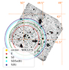 |
Fig. 7. Residual image in the IE field of the Perseus cluster (after ICL subtracting): The centres of elliptical (E) galaxies are marked with red dots, S0 galaxies with green dots, intermediate types between S0 and spirals with cyan dots, and spirals with dark blue dots. Coloured circles, centred on the central elliptical galaxy NGC 1275, indicate the average projected distance for each morphological type. |
In addition, Table 2 shows the number of galaxies and the mean Sérsic index for a single-Sérsic model used in the catalogue from Cuillandre et al. (2025b) for each morphological group. We note that the average Sérsic index increases slightly with the morphological group, which is consistent with our classification. Appendix E provides some plots validating this morphological classification.
Distribution of disc galaxy morphology in our sample.
2.6. Influence of other parameters
The sample was also characterised by its mass distribution, determined in Cuillandre et al. (2025b). The disc galaxies have masses in the range log10(M*/M⊙)∈ [7.7, 11.3] with a median value of log10(M*/M⊙) = 9.92.
The link between profile type and galaxy mass is now studied through classification into three bins, each containing 34 disc galaxies. This arbitrary choice delivers meaningful statistics for each bin given the small number of objects.
Considering the fact that the role of the environment is highly debated in the literature, as indicated previously, we adopt in our study four distinct regions within the 0.7 deg2 field of view of Perseus. They are defined in the RA/Dec plane using a kernel density estimation (KDE) plot, i.e. the gaussian_kde function. This approach allows us to visualise the global distribution of cluster galaxies, considering bright and faint dwarf galaxies. Each galaxy counts as one in this KDE plot and is not weighted by mass in order to only take into account spatial distributions. For more details on the distribution of dwarfs, we refer the readers to Marleau et al. (2025). Analysing the density contours generated by the KDE plot enables a more precise characterisation of the spatial distribution of galaxies within the defined regions, as depicted in Sect. 3.2.1.
3. Characterisation of the disc breaks
Our global sample is thus characterised in terms of morphologies and profile types. This section now describes down- and up-bending break discs in more detail. Specifically, the parameters of the double exponential fitting are first characterised. Finally, the influence of the environment will be studied through other parameters such as mass and morphology.
3.1. Parameters of the break
Tables 3 and 4 provide the mean and median parameters of Eq. (3) in our sample, both for the down-bending double, meaning Type II, and the up-bending, meaning Type III, double exponential profiles respectively. The uncertainties associated with the mean and median values correspond to the standard deviation within our sample. This characterisation allows for the identification of the break occurring for Type II and Type III profiles around magnitude 25, as hinted in Laine et al. (2016). Type III profiles show a slightly higher average and median surface brightness at the break compared to Type II profiles. However, when considering the scatter, this difference is not statistically significant. In addition, the average and median break radius for both Type II and Type III profiles is approximately equal to the radius at magnitude 25 in the visible, which is consistent with previous results (Laine et al. 2016). Figure 8 illustrates the normalised surface brightness profiles for the different profile types in our sample. To construct the median profiles, each individual galaxy profile was first normalised in radius: by the break radius Rbreak for Type II and Type III galaxies, and by the isophotal radius R25 for Type I galaxies. Each normalised profile was then interpolated onto a common radial grid spanning from 0 to 1.5 in units of the normalisation radius. It highlights the distinct characteristics of Type II, Type III, and Type I profiles, alongside a combined view of their median profiles. For Type II profiles (top left panel), the break is marked by a down-bending transition, consistent with break disc observed in previous studies. In contrast, Type III profiles (top right panel) display an up-bending transition, indicative of an extended outer disc structure. The bottom left panel shows Type I profiles, where no significant break is evident. The combined median profiles (bottom right panel) reinforce the typical trends for each profile type, with shaded regions indicating the variability among individual profiles within each category.
Parameters of the double exponential model for the four identified down-bending disc breaks (Type II) in our sample.
Parameters of the double exponential model for the 24 identified up-bending disc breaks (Type III) in our sample.
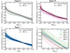 |
Fig. 8. Distribution of normalised surface brightness profiles for different types of galaxies. The subplots show the profiles for Type II (top left), Type III (top right), Type I (bottom left), and the combined median profiles for the three types around R = Rnorm (bottom right). Individual profiles are displayed with a colour gradient, while the median profile is represented in black. The shaded region around the median indicates the 68% confidence interval, reflecting the variability among individual profiles. Note that Rnorm corresponds to R25 for Type I or Rbreak for Type II and III. |
As indicated in previous studies (van der Kruit 1988; Pohlen & Trujillo 2006; Comerón et al. 2012; Laine et al. 2016), the plane displaying the ratio of the break radius to the first disc scalelength (Rbreak/hd1) as a function of the ratio between the disc scalelengths (hd1/hd2) is widely used to distinguish between down- and up-bending disc breaks. Figure 9 shows the distribution of down- (in green) and up-bending break (in pink) profile parameters in this space, clearly identifying the Type II and Type III groups. In this diagram, as expected, for up-bending break profiles (in magenta), we observe hd2 > hd1, meaning the slope decreases beyond the break radius, while for down-bending break profiles (in green), we see hd2 < hd1, indicating that the slope increases beyond the break.
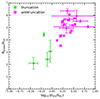 |
Fig. 9. Ratio of the truncation radius to the first disc scalelength (Rbreak/hd1) as a function of the logarithm of the ratio between the disc scalelengths (hd1/hd2). This plot visually separates Type II galaxies (green dots) from Type III galaxies (magenta dots). The error bars are directly extracted from the uncertainties on the parameters obtained during the surface brightness profile fitting process. |
An interesting observation is that, on average, Rbreak/hd1 is smaller for down-bending disc breaks compared to up-bending ones. This is consistent with the findings of Comerón et al. (2012), who noted that thick discs tend to truncate at lower relative radii than thin discs, likely due to the longer inner scalelength of the thick disc. Pohlen & Trujillo (2006) reported that the break typically occurs at about 2.5 times the inner scalelength (hd1), with a surface brightness of μbreak ∼ 23.5 mag arcsec−2 for Type II galaxies. In contrast, Type III galaxies exhibit breaks further out, at about 4.9 times the inner scalelength, with a lower surface brightness of μbreak ∼ 24.7 mag arcsec−2.
Our results are broadly consistent with these trends, although we find that for Type II galaxies, the break occurs at a slightly larger radius, approximately 2.9hd1 on average, and at a fainter surface brightness of μbreak ∼ 24.5 mag arcsec−2. For Type III galaxies, we observe a break radius of approximately 5.2hd1 on average, with an even lower surface brightness of μbreak ∼ 25.3 mag arcsec−2. These differences may reflect variations in sample selection or environmental factors but confirm the general trend that down-bending disc breaks occur at smaller radii with brighter surface brightness, while up-bending disc breaks are found further out in regions with fainter surface brightness.
Note that we provide in Appendix F the distributions of all fitting parameters for Type II and Type III profiles.
3.2. Role of the cluster environment
Early studies, such as those by Pohlen & Trujillo (2006), revealed no significant differences between field and cluster galaxies, potentially due to variations in sample selection. However, more recent research presents a contrasting view, suggesting that galaxy types are significantly shaped by their environments. For instance, Laine et al. (2016) conducted analyses on similar galaxy populations across varied settings, including both field and cluster environments like the Virgo cluster. This research highlighted a statistically significant correlation between the inner and outer disc scale lengths and the Dahari parameter2, which measures the strength of gravitational interactions between a galaxy and its nearby companions. This correlation is particularly notable in Type III and Type I profiles, indicating that interactions within the cluster might play a crucial role in shaping these profiles. Further supporting this perspective, Pranger et al. (2017) demonstrated that the prevalence of each galaxy type varies considerably with environmental factors.
To investigate the role of the Perseus cluster environment more precisely, we aim to cover the nuanced impact of the cluster on galaxy evolution. We explore the spatial position of down- and up-bending break galaxies in Sect. 3.2.1, as well as the effects of morphological types in Sect. 3.2.2 and mass in Sect. 3.2.3.
3.2.1. Spatial distribution of profile type
We first study in this section the spatial distribution of the different profile types so as to provide insights into how environmental conditions within the cluster influence their shape. To illustrate this, a gaussian KDE plot was created to visualise the distribution of the complete catalogue, which includes both dwarf and bright galaxies, in the right ascension versus declination plane, as shown in Fig. 10. The limits of the colourbar, and consequently the bins, are dynamically calculated based on the probability densities estimated over the entire set of massive galaxies. It is important to note that only four bins are chosen to ensure statistically meaningful results. The four probability density bins are depicted with colours ranging from intense red, marking the core of the cluster, to pale yellow, describing the outskirts. On top of this density visualisation, we overlay the specific positions of Type II (green dots) and Type III (magenta dots) galaxies. This method shows us with a detailed analysis of how the spatial distribution correlates with different profile types. Figure 10 shows indeed that both down-bending break Type II and Type III profiles appear to be present throughout the cluster. Type I galaxies (profiles without breaks) initially dominate, representing approximately 80% of the population in the innermost bin. This fraction slightly increases in the second bin but then decreases towards the cluster outskirts, where Type I galaxies make up only about 50% of the population. This shift suggests that Type I profiles, initially predominant in the cluster’s central regions, gradually become less common in the outer parts. Type III galaxies appear to be more uniformly distributed throughout the cluster. We note a small trend that Type III galaxies show a tendency to avoid the cluster core, as suggested in Fig. 10. Their population increases in the outskirts, supporting the idea that environmental effects in the cluster centre may inhibit the processes leading to the formation or survival of up-bending break profiles. In contrast, the spatial distribution of Type II galaxies shows a more concentrated pattern, with three out of four Type II galaxies located in the core of the cluster and only one in the periphery. This peripheral Type II galaxy might suggest distinct characteristics compared to its counterparts in the core, potentially exhibiting additional features such as a bar structure or other morphological peculiarities. These differences in spatial distribution may hint at varying formation and evolutionary processes for Type II and Type III galaxies within the cluster. It is important to note, however, that the number of galaxies is small, especially for Type II.
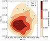 |
Fig. 10. Kernel density estimation plot of the distribution of the complete catalogue (dwarfs + bright galaxies) in the right ascension versus declination plane: four probability density bins are indicated in colour, showing higher probability density in the centre in red and lower density in the outskirts in pale yellow. Dots are overplotted on this distribution to indicate the positions of Type II galaxies in green and Type III galaxies in magenta. The black cross indicates the centre of NGC 1275. |
One step further in this analysis, Fig. 11 shows the fraction of each profile type within the total population of spiral to S0 galaxies, highlighting the variations from the core (dark red) to the outer regions (yellow). This detailed breakdown allows for an examination of how the prevalence of different profile types varies with their location within the cluster, further quantifying the impact of environmental conditions on galaxy evolution. Overall, Type I galaxies are prevalent (75%), while roughly between 20 and 25% are up-bending break profiles, and a few percent down-bending break profiles. This distribution indicates that while non-down-bending break profiles are the most numerous, up-bending break profiles also constitute a significant proportion of the population, and down-bending break profiles are less common but still present across the cluster. More precisely, when examining these same fractions across different probability density bins, it is observed that the fraction of up-bending break profiles, meaning Type III, slightly increases as we move away from the central bin. In the outermost bin, Type III profiles account for about 40% of disc galaxies. Conversely, for Type II profiles, there are three down-bending break profiles in the core and one down-bending break profile in the outer region. However, despite the small statistics, down-bending break profiles (Type II) are present both in the core and the outer regions, which contrasts with earlier conclusions suggesting the absence of Type II profiles in clusters like Virgo (Erwin et al. 2012). The presence of Type II profiles in our study aligns more closely with the findings of Laine et al. (2016) and Head et al. (2015), who showed that down-bending disc breaks can persist even in dense environments such as the core of the Coma cluster. Finally, it is important to note that our density bins are defined in projection, meaning that some objects classified in the core bin could actually be located at significant distances from the centre in 3D space. This distinction is crucial when interpreting the spatial distribution of profile types within the cluster.
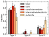 |
Fig. 11. Fraction of each type within the total population of spiral to S0 galaxies: Type I, Type II and Type III. The grey bars indicate the total fraction of each type. The coloured bars, ranging from dark red to pale yellow, show the fraction of each type within each region from the core to the outer regions. Error bars represent the 1σ binomial uncertainties calculated as |

3.2.2. Morphological influence
Let us now turn to the role of morphological types. As indicated in Sect. 2, we define three classes of discs, ranging from S0 galaxies (type = − 1) to spirals (t = 1). Figure 12 shows the evolution of the total fraction of each profile type with the associated morphological type, regardless of the cluster position. It is observed that Type I profiles dominate in fraction across all galactic morphologies. However, this fraction is slightly higher for spirals compared to the other morphological types. On the other hand, the fraction of Type III profiles is slightly lower for spirals. The proportion of Type II profiles appears relatively consistent across different morphological types, though the small sample size warrants caution in drawing definitive conclusions.
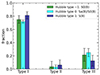 |
Fig. 12. Fraction of galaxies in each density bin for each Type profiles for the different Hubble morphological type: one corresponds to spirals (darkblue), zero to S0/spiral intermediates (cyan), and minus one to confirmed S0 galaxies (green). Error bars represent the 1σ binomial uncertainties calculated as |

Aiming at studying the interplay between profile types and both morphology and environment, we display in Fig. 13, the abundance of Type I, II, III across the different probability density bins for each galaxy morphology. In the left panel, the fraction of Type III profiles for S0 galaxies is shown to dominate in the outermost region of the cluster compared to Type I profiles. In this region, Type II profiles are not present for S0 galaxies. For spiral galaxies, Type II profiles are found in the cluster core, while Type I and Type III profiles are more common in the lower density bins.
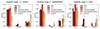 |
Fig. 13. Fraction of each profile type (I, II, III) according to the angular projection within the cluster (from red to yellow) similar to Fig. 11 but for different galaxy morphology from Hubble type −1 on the left-hand panel, to one on the right-hand panel. Error bars represent the 1σ binomial uncertainties calculated as |

With respect to both spatial distribution and morphological characteristics within the cluster, differences are observed between different morphologies but no significant general trend emerges.
3.2.3. Mass influence
We now turn to the potential correlations between the mass of disc galaxies and the proportion of each profile type. Figure 14 presents the mass distribution of disc galaxies across galaxy density bins within the cluster. Although asymmetry appears in the distributions, the mean and median disc masses remain fairly consistent across bins. Examining a rolling mean over 10 galaxies reveals a slight decrease in mass from denser regions to the outskirts, though this trend in mean/median mass is weak. Notably, the distribution tails indicate that the most massive galaxies are preferentially located closer to the cluster centre, consistent with a general trend of mass segregation. van der Burg et al. (2018) discuss how massive galaxies are commonly found near the core, while lower-mass galaxies dominate the outer regions.
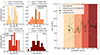 |
Fig. 14. Stellar mass distribution of galaxies according to their position in the cluster. Left-hand panel: stellar mass distribution of galaxies across the different environments (from outskirts – top left panel – to core – bottom right panel), each represented by a different colour as labelled. Right-hand panel: galaxy mass as a function of probability density, with individual galaxies represented by grey dots. The black curve indicates the rolling average over 10 galaxies, black squares show the mean, and green dots represent the median for each density bin. The error bars corresponds to the standard error on the mean and median. |
This mass segregation may result from various gravitational and dynamical processes: dynamical friction, for example, might cause massive galaxies to lose orbital energy over time, drawing them towards the cluster centre (Chandrasekhar 1943). Additionally, while high velocities inhibit mergers in dense cores, slower encounters at the outskirts could lead to accretion and central galaxy growth (Merritt 1985). Recent studies support this mass-dependent distribution; for instance, Barsanti et al. (2016) observed lower velocity dispersions for massive galaxies, suggesting that dynamical interactions influence their central distribution. However, within the innermost regions, particularly within 0.25R200, mass variations are modest, with only slightly more massive galaxies at the centre. This suggests a relatively homogeneous stellar mass population in dense cluster cores, consistent with a gradual gradient in mass segregation at small scales (Haines et al. 2015).
In our sample within 0.25R200, within the Euclid field of view (Cuillandre et al. 2025b), the mass distribution follows this pattern, showing a weak but noticeable gradient in stellar mass outwards, as described Fig. 14. This aligns with expectations that gravitational and environmental processes, such as dynamical friction or tidal stripping, tend to homogenise the mass distribution in the densest cluster regions, resulting in a modest overall mass variation within 0.25R200.
Subsequently, three mass bins were defined, each containing an equal number of disc galaxies. The fractions of each profile type within each mass bin were then analysed, as shown in Fig. 15. The overall trend shows minimal variation in the fractions across different probability density bins, specifically different environments. For low-mass galaxies, the general trend observed globally is similar to our results of Sect. 3.2.1, with a slightly decreasing number of Type I profiles and an increasing proportion of Type III profiles in the less dense, outer regions of the cluster. Type II profiles, however, are confined to the cluster core and constitute a small overall fraction. For high-mass galaxies, the same trend is observed but is less pronounced: in the outer regions, Type III profiles represent 40% of the profiles, a value that rises to 50% in the first mass bin. For intermediate-mass galaxies, the correlation is less clear. In the first three denser bins near the centre, the fractions remain relatively constant. Nevertheless, it is notable that down- and up-bending break profiles collectively constitute nearly 50% of all profiles in the outermost probability density bin. These findings are consistent with recent studies (O’Kane et al. 2024) showing that stellar masses tend to be higher in denser environments, such as the cluster core, although the differences are relatively modest compared to other environments, such as groups or the cluster outskirts. In summary, the most massive galaxies, as well as the more evolved morphological types, are concentrated near the cluster centre, as expected.
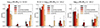 |
Fig. 15. The fraction of each profile type (I, II, III) according to the angular projection within the cluster (from red to yellow) similar to Fig. 11 but for three different stellar mass bins from left/lower masses to right/larger masses as labelled. Error bars represent the 1σ binomial uncertainties calculated as |
However, we must highlight that the statistical significance of these present results is limited, and the differences observed here should be interpreted with caution, as they may not be very significant due to the small sample size. A clearer result could be expected if the 2D distribution could be deprojected into 3D.
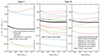 |
Fig. 16. Normalised magnitude difference IE− HE as a function of radius R/Rbreak for galaxies Type II, Type III and Type III with a detected U-shaped profile. The profiles are normalised around R = Rbreak. The minimum value within the range 0.5 ≤ R/Rbreak ≤ 1.5 is identified. |
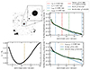 |
Fig. 17. Profile of the galaxy SDSS 1237661122387969061. Top Left Panel: Image of the galaxy with associated radii indicated by ellipses of different colours: green/yellow for the break positions in the surface brightness profiles of IE (μIE) and HE (μHE) bands, red for the radius at |


3.2.4. Colour gradients as a function of radius
Our observations in the NIR in the HE-band allow us to map these regions of outer discs in more detail than previous optical studies, such as those by Zheng et al. (2015), which were often limited in depth. NIR data provide a unique view of LSB regions dominated by older stars. At these wavelengths, the effects of dust extinction are minimised, and the mass-to-light ratio remains more stable, offering a clearer indication of stellar mass. Unlike optical studies, which are heavily influenced by younger stars with high luminosity/mass ratios, our NIR data more accurately reflect the mass distribution of the galaxy. This red gradient, therefore, indicates older and redder stellar populations in the peripheries of galaxies (Bakos et al. 2008; Zheng et al. 2015; Watkins et al. 2016). This approach offers two main advantages. First, focusing on older stellar populations in the outer disc creates a smoother profile, facilitating the identification of structures such as upturns and downturns in disc breaks. The U-shaped profiles observed in some galaxies underscore this effect, revealing an age gradient across the disc, with older and redder populations concentrated in the peripheries. Secondly, by working in the NIR, we avoid some of the complex corrections required in optical data for estimating stellar mass, where dust extinction and age-related luminosity variations can complicate direct mass mapping. Additionally, Zheng et al. (2015) shows that, across different Hubble types, galaxies tend to have simple exponential mass profiles, indicating that these variations reflect differences in stellar populations rather than changes in mass distribution.
Figure 16 presents the normalised IE-HE colour profiles of Type II and Type III galaxies. As the left panel shows, among the Type II galaxies studied, only one exhibits a U-shaped colour profile, characterised by a marked colour gradient. This finding is significant as it indicates a relatively low occurrence of this phenomenon in Type II galaxies, which is lower than the frequency generally reported in cluster studies, such as that by Roediger et al. (2012). The consensus is that this U-shape comes from the stellar radial migration (Roškar et al. 2008a). Moreover, Fig. 16 reveals that among Type III galaxies, six of them, or one quarter, exhibit U-shaped colour profiles. This observation is particularly interesting as it suggests additional complexity in the evolutionary processes of Type III galaxies. Roediger et al. (2012) demonstrates that U-shaped galaxies can be present for all three types, although it is primarily Type II galaxies that are predominantly of this shape. Xu & Yu (2024), who have recently been exploring discs at higher redshifts, confirm that U-shaped profiles are not exclusive to Type II galaxies but also exist for Type III. Figure 17 provides an example of a galaxy with an upward curvature break profile and its strong U-shape. We observe that the break in the profile 17 occurs before the expected break, as indicated by Bakos et al. (2008). We observe that the break in the profile, marked by the green dotted line in the top left panel, is around 0.7Rbreak, indicated by the golden dotted line in the reddest NISP band, the HE band. This is also the case for two other galaxies in purple and brown on the right panel of Fig. 16. However, most of these U-shapes, four out of six, are not very strong and thus only show a small colour gradient, tending towards a plateau, a known feature highlighted by Bakos et al. (2008). Thus, the few Type III discs observed could be the result of recent star formation in the outer regions of the disc, as suggested by Xu & Yu (2024). The others have rather a plateau profile after a minimum or a slight decrease, as shown in the middle panel of Fig. 16 and expected by Bakos et al. (2008), Roediger et al. (2012), and Zheng et al. (2015).
These observations in NIR represent a step forwards in probing LSB regions in nearby galaxies, making it possible to reach the faint outermost regions of galactic discs with greater precision. By mapping the distribution and mass of these older stellar populations, this dataset provides a more refined perspective on the outer structures of galaxies and the evolutionary mechanisms shaping them, such as radial migration and satellite accretion.
4. Discussion
In this section, we discuss our findings on galaxy disc profile types within the Perseus cluster and compare them with results from both simulations and other clusters. Our observations reveal possible trends in the presence of Type II and Type III profiles in this cluster environment, potentially shaped by both internal dynamics and the external cluster environment. These findings highlight the role of galaxy-cluster interactions in shaping galaxy morphology, supporting or challenging various theoretical interpretations and previous observational results.
4.1. Comparison to simulations of galaxy-cluster interaction
To understand the rarity of Type II profiles within the Perseus cluster, contrasted with their frequency in field surveys, and the persistence of Type III profiles in this environment, we use results from a series of simulations (Mondelin et al. in prep., hereafter Paper II). These simulations start with disc galaxies displaying a Type I, II, or III profile, formed through internal instabilities at high redshift (z between one and three). A Type II disc galaxy, for example, remains stable in isolation, with its radial break intact over a few billion years. However, when subjected to the tidal forces of a Perseus-like cluster, this truncation weakens, leading the galaxy to adopt a Type I profile within one or two cluster crossing times (i.e. at most 1 or 2 Gyr).
The results of these simulations, summarised in Fig. 18, show that the transition from Type II to Type I profiles results primarily from the disturbance of stellar orbits, which become more elongated, and from the triggering of star formation in the galaxy’s outer disc by the cluster’s tidal field. This suggests that the cluster environment can indeed inhibit Type II profiles, aligning well with our observations in the Perseus cluster. Thus, our findings provide observational support for the idea that Type II discs may be transformed or erased by cluster interactions, while Type III discs can survive due to different physical mechanisms.
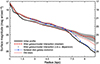 |
Fig. 18. Hydrodynamical simulations of the interaction of a Type II galaxy with a Perseus-like cluster. The initial disc galaxy (solid black curve) has a double exponential, Type II radial profile, and a central bulge, formed by disc instabilities at high redshift, with a break at 6.5 kpc and a gas fraction of 17% in the disc. These initial conditions are taken from simulations of high-redshift disc instabilities and Type II profile formation in Bournaud et al. (2007). Simulations (Paper II) evolve this disc galaxy in the tidal field of the Perseus-like cluster for about one cluster crossing time. The median profile over six simulated orbits (red dashed curve) and the RMS dispersion (shaded area) are displayed, showing that the galaxy evolves most of the time towards a Type I disc, while the same galaxy in isolation during the same timescale would remain Type II (thin blue line with diamonds). Stars pre-existing to the galaxy/cluster interaction (red dotted line) are scattered radially over increasingly eccentric orbit, accounting for about two thirds of the replenishment of the outer disc beyond the initial break radius, the other third coming from the triggering of turbulence, shocks, and star formation in the outer disc by the tidal field of the cluster (see Paper II for individual orbits and detailed interpretation). |
4.2. Comparison to other works
We now turn to how our findings on disc profiles in the ERO-Perseus field compare with previous observational studies and theoretical models, especially regarding the environmental factors that influence profile transformations.
4.2.1. Down-bending disc break profile
Our study identified a few Type II galaxies (4), a number which is relatively low compared to field surveys, aligning with other cluster studies, such as Erwin et al. (2012), which found no Type II profiles within the Virgo cluster core. As we have also verified using hydrodynamical simulations in Sect. 4.1, this scarcity in dense environments suggests that Type II profiles may struggle to survive cluster conditions.
Moreover, approximately 25% of the galaxies observed in the 2D inner bins actually originate from the outskirts in 3D, assuming an isotropic distribution. This finding emphasises the need for incorporating precise 3D measurements, such as spectroscopic redshifts and velocity measurements, corrected for projection effects like the finger-of-god effect, in order to confirm whether Type II profiles genuinely survive the harsh conditions of dense cluster environments.
However, if we consider that some Type II galaxies do survive within Perseus’ inner regions, it is likely due to certain stabilising effects. Structural features, such as bars, may have a significant role in maintaining their persistence (Elmegreen & Elmegreen 2014). Figure 19 presents IE images of four galaxies with down-bending disc breaks, where structures like bars and outer Lindblad resonances (OLR) appear to contribute to their stability for at least two of them. For example, the galaxy WISEA J031637_12+414721_3 shows evidence of a recent bar formation, suggesting that such features might help retain a down-bending break profile even in the cluster’s core. Notably, UGC 02665 displays clear signs of truncation likely due to ram pressure stripping, where it is losing gas and stars as it moves through the cluster. The different truncation mechanisms observed hint at a variety of structural and environmental interactions contributing to the persistence or suppression of Type II profiles in the Perseus cluster.
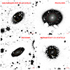 |
Fig. 19. IE LSB images of four down-bending break galaxies. The truncation is indicated by the green dashed ellipse, i.e the isophote with a semi-major axis equal to that of the break. The outer region lies beyond this isophote. The red ellipse denotes the radius at μIE = 25 mag arcsec−2. We note that the red circle is close to the green circle. The line at the bottom right of each image gives the scale, which corresponds to 10″. |
These observations in Perseus are consistent with trends in the Coma cluster, where bars have also been linked to the formation and maintenance of broken discs (Head et al. 2015). However, comparisons with Virgo and Coma reveal that the proportions of Type II and Type III profiles vary between clusters, suggesting that local environmental conditions and assembly histories could influence profile distribution. Moreover, Pranger et al. (2017) compared spiral galaxies in clusters and those in the field and shows that the fraction of Type I galaxies is higher in clusters, while the fraction of Type II galaxies is lower compared to the field. Specifically, Type I galaxies are approximately 2.5 times more frequent in clusters than in the field, which is in agreement with our observations.
4.2.2. Up-bending disc break profile
We observe that about a third of the Type III galaxies in Perseus display U-shaped colour gradients, indicating older stellar populations in the outer regions, which may be due to radial migration or accretion. This finding aligns with those in other clusters, such as Virgo (Erwin et al. 2012), where a mix of Type I and Type III profiles was found. Interestingly, we observe a location-dependent variation in Perseus, with Type III profiles representing about 20% in the cluster core but up to 40% in the outskirt, as shown in Fig. 11. This gradient could be due to environmental effects, though detecting up-bending disc breaks near the cluster centre remains challenging due to the high density of galaxies.
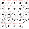 |
Fig. 20. IE LSB images of up-bending break galaxies. The break is indicated by the green dashed ellipse, i.e the isophote with a semi-major axis equal to that of the break. The red ellipse denotes the radius at μIE = 25 mag arcsec−2. We note that the red circle is close to the green circle, in most of the cases. The line at the bottom right of each image gives the scale, which corresponds to 10″. |
Pranger et al. (2017) found that the fraction of Type III galaxies remains consistent between cluster and field environments. Interestingly, they observed that Type III cluster galaxies tend to reside significantly closer to the cluster centre compared to other break types. This finding contrasts with our observations in Perseus, where we see a higher proportion of Type III profiles in the cluster outskirts compared to the core. However, it is important to note that our observations are limited to within 0.25 R200 of Perseus, and we lack statistical data for regions beyond this radius. Moreover, Sánchez-Alarcón et al. (2023) shows that in more isolated environments, there are mainly Type II and I profiles, and that Type III profiles are primarily due to interactions, such as major mergers. This is consistent with our results where the number of Type II profiles is low for cluster galaxies and Type III profiles are numerous, potentially due to their merger history and frequent interactions in a dense environment such as Perseus.
In the Coma cluster, Type III profiles are frequently associated with bars, with nearly 71% of these galaxies displaying this feature. By contrast, barred Type III galaxies in Perseus are almost absent, as shown in Fig. 20. This discrepancy suggests that while bars are essential for broken discs in Coma, other mechanisms, such as minor mergers or accretion, might be more relevant in Perseus. Notably, Chamba & Hayes (2024) find that Type III profiles often correlate with extended H I reservoirs and smoother H I gradients, highlighting the role of gas dynamics in shaping these profiles. Extended H I reservoirs provide material for star formation in the outer disc, while smoother gradients facilitate stellar redistribution via radial migration, contributing to the observed U-shaped colour gradients. External processes, such as minor mergers or satellite interactions, can also drive the formation of up-bending break profiles. Future spatially resolved H I observations of Perseus could further illuminate the connection between gas reservoirs and the persistence of Type III profiles in cluster environments.
The Coma study also links up-bending break discs to bulge growth, likely driven by mergers or starbursts, supporting the view that Type III profiles can result from significant internal restructuring. Our findings in Perseus, particularly the prevalence of older stellar populations, align with this hypothesis. The comparison to previous studies further reinforces that Type II profiles are typically suppressed in dense environments, while Type III profiles remain more stable, likely sustained by mechanisms such as radial migration or mergers. The differing proportions of Type III profiles across Perseus, Coma, and Virgo may be linked to the clusters’ dynamical states and formation histories. For instance, the lack of barred Type III galaxies in Perseus compared to Coma might reflect differences in the role of secular processes in more virialised clusters. Meanwhile, Virgo’s ongoing accretion of substructures could create an environment where gas accretion and minor mergers dominate the formation of up-bending break profiles. Future studies combining detailed stellar population analyses and H I maps could provide further insights into how these histories influence the evolution of galaxy profiles.
Our methodological approach, employing AutoProf/AstroPhot and high-resolution, wide-field Euclid images, allows for improved profile detection, even in dense regions like the Perseus core. This approach contrasts with methods used in previous studies, such as the IRAF task ellipse and GALFIT, which are effective but, as AutoProf, limited in crowded cluster environments. By achieving greater precision in profile identification, especially at faint magnitudes, we expand our understanding of galaxy morphology across cluster environments.
5. Conclusions
In this work, we have studied the distribution and characteristics of galaxy profiles within the Perseus cluster, focusing on the roles of mass, bars, and morphology. The main findings can be summarised as follows.
-
Type II profiles: Among the 102 massive disc galaxies identified in the Perseus cluster, we classified 74 as Type I, four as Type II, and 24 as Type III. Of the Type II galaxies, three are projected close to the cluster core, within a few hundred kiloparsecs of the central galaxy. Bars and specific resonance effects, such as the OLR, were found in two out of the four Type II galaxies, suggesting that they may play a role in stabilising these down-bending break profiles, even in the dense cluster environment. However, it is important to consider that older processes, such as previous interactions or internal dynamics, might have caused breaks that could have been erased upon entering the cluster. The harsh conditions of the cluster, such as tidal forces or ram pressure stripping, may lead to a smoothing of the surface brightness profile, masking older breaks. Additionally, if the truncation is related to a threshold effect in star formation, or to ram pressure stripping of the outer gas, this would more prominently affect the colours of the galaxy. Specifically, the region beyond the break would appear old and red due to the cessation of star formation. These aspects suggest that both the age of the stellar populations and the colour profiles are critical in understanding the origin and persistence of Type II profiles in cluster environments. Moreover, as mentioned in Sect. 4.1, simulations of Type II profiles in a cluster context reveal the role of the cluster’s gravitational potential, explaining the low fraction of this Type In the Perseus cluster. In Paper II, we aim to describe and further develop these simulations, with the goal of demonstrating how initial conditions – such as the star formation threshold or the entry orbit into the cluster – can significantly explain the observed variations in profile types.
-
Type III profiles: Approximately one quarter of the Type III galaxies in the Perseus cluster show a small U-shaped colour gradient with a minimum around 0.7Rbreak, indicative of older star populations in the outer regions. Unlike the Coma cluster, where bars are commonly associated with broken discs, no visibly barred Type III galaxies were confirmed in Perseus. This suggests that other mechanisms, such as mergers and radial migration, may be more significant in the formation of up-bending break profiles in this cluster.
-
Role of mass and morphology: The study also underscored the influence of galaxy mass and morphology on profile types. The spatial distribution of these profiles varies, with certain morphological types and mass ranges more prevalent in specific regions of the cluster. In particular, it was observed that more massive galaxies tend to have more complex structures and profile types. This is consistent with the notion that massive galaxies are more likely to have undergone significant interactions and mergers, which can lead to the formation of diverse structural components such as bulges and extended discs. The distribution of mass within the cluster also appears to influence the types of profiles observed, with less massive galaxies being more susceptible to environmental effects like ram pressure stripping.
-
Spatial distribution: The findings suggest that while the overall frequency of Type II galaxies may decrease in clusters, certain stabilising factors, such as the presence of bars and specific resonance effects, can maintain these profiles even in harsh conditions. The spatial distribution of profiles within the cluster reflects the complex interplay between internal dynamics and environmental influences.
These findings highlight the diversity of mechanisms that can lead to the formation and stabilisation of Type II profiles, even in dense cluster environments. While the overall frequency of Type II galaxies may decrease in clusters, certain stabilising factors, such as the presence of bars and specific resonance effects, can maintain these profiles even in harsh conditions. Further studies, including 3D spatial analysis, would be necessary to confirm the true position and resistance of these galaxies within the cluster. Extending the study to a larger field around the cluster would provide more statistical power and help clarify the broader environmental influences on galaxy evolution. Additionally, acquiring 3D velocity maps would allow for a non-projected representation of galaxy positions, offering more precise insights into their true local environment. Although this is currently challenging due to the dominant effect of galaxies’ proper motions within the cluster, the upcoming Euclid DR1 data release will allow us to expand the field of view, enabling analysis of galaxies in less dense environments as well. This will provide a valuable comparison to cluster environments and deepen our understanding of the environmental factors shaping galaxy evolution.
Acknowledgments
This work has made use of the Early Release Observations (ERO) data from the Euclid mission of the European Space Agency (ESA), 2024, https://doi.org/10.57780/esa-qmocze3. The Euclid Consortium acknowledges the European Space Agency and a number of agencies and institutes that have supported the development of Euclid, in particular the Agenzia Spaziale Italiana, the Austrian Forschungsförderungsgesellschaft funded through BMK, the Belgian Science Policy, the Canadian Euclid Consortium, the Deutsches Zentrum für Luft- und Raumfahrt, the DTU Space and the Niels Bohr Institute in Denmark, the French Centre National d’Etudes Spatiales, the Fundação para a Ciência e a Tecnologia, the Hungarian Academy of Sciences, the Ministerio de Ciencia, Innovación y Universidades, the National Aeronautics and Space Administration, the National Astronomical Observatory of Japan, the Netherlandse Onderzoekschool Voor Astronomie, the Norwegian Space Agency, the Research Council of Finland, the Romanian Space Agency, the State Secretariat for Education, Research, and Innovation (SERI) at the Swiss Space Office (SSO), and the United Kingdom Space Agency. A complete and detailed list is available on the Euclid web site (http://www.euclid-ec.org). Fernando Buitrago acknowledges support from the GEELSBE2 project with reference PID2023-150393NB-I00 funded by MCIU/AEI/10.13039/501100011033 and the ESF+. The authors thank Mireia Montes for their useful comments and discussions.
References
- Allen, P. D., Driver, S. P., Graham, A. W., et al. 2006, MNRAS, 371, 2 [Google Scholar]
- Bakos, J., Trujillo, I., & Pohlen, M. 2008, ApJ, 683, L103 [NASA ADS] [CrossRef] [Google Scholar]
- Barsanti, S., Girardi, M., Biviano, A., et al. 2016, A&A, 595, A73 [NASA ADS] [CrossRef] [EDP Sciences] [Google Scholar]
- Belokurov, V., Erkal, D., Evans, N. W., Koposov, S. E., & Deason, A. J. 2018, MNRAS, 478, 611 [Google Scholar]
- Bertin, E., & Arnouts, S. 1996, A&AS, 117, 393 [NASA ADS] [CrossRef] [EDP Sciences] [Google Scholar]
- Borlaff, A., Eliche-Moral, M. C., Rodríguez-Pérez, C., et al. 2014, A&A, 570, A103 [NASA ADS] [CrossRef] [EDP Sciences] [Google Scholar]
- Borlaff, A., Eliche-Moral, M. C., Beckman, J. E., et al. 2017, A&A, 604, A119 [NASA ADS] [CrossRef] [EDP Sciences] [Google Scholar]
- Bournaud, F., Elmegreen, B. G., & Elmegreen, D. M. 2007, ApJ, 670, 237 [Google Scholar]
- Buitrago, F., & Trujillo, I. 2024, A&A, 682, A110 [NASA ADS] [CrossRef] [EDP Sciences] [Google Scholar]
- Chamba, N., Hayes, M. J., & LSST Dark Energy Science Collaboration. 2024, A&A, 689, A28 [NASA ADS] [CrossRef] [EDP Sciences] [Google Scholar]
- Chandrasekhar, S. 1943, ApJ, 97, 255 [Google Scholar]
- Comerón, S., Elmegreen, B. G., Salo, H., et al. 2012, ApJ, 759, 98 [CrossRef] [Google Scholar]
- Cuillandre, J.-C., Bertin, E., Bolzonella, M., et al. 2025a, A&A, 697, A6 [Google Scholar]
- Cuillandre, J.-C., Bolzonella, M., Boselli, A., et al. 2025b, A&A, 697, A11 [Google Scholar]
- de Vaucouleurs, G. 1948, Ann. Astrophys., 11, 247 [Google Scholar]
- Debattista, V. P., Mayer, L., Carollo, C. M., et al. 2006, ApJ, 645, 209 [Google Scholar]
- Dressler, A. 1980, ApJ, 236, 351 [Google Scholar]
- Eliche-Moral, M. C., González-García, A. C., Balcells, M., et al. 2011, A&A, 533, A104 [NASA ADS] [CrossRef] [EDP Sciences] [Google Scholar]
- Elmegreen, D. M., & Elmegreen, B. G. 2014, ApJ, 781, 11 [Google Scholar]
- Elmegreen, B. G., & Hunter, D. A. 2006, ApJ, 636, 712 [NASA ADS] [CrossRef] [Google Scholar]
- Elmegreen, B. G., & Struck, C. 2013, ApJ, 775, L35 [NASA ADS] [CrossRef] [Google Scholar]
- Erwin, P., Beckman, J. E., & Pohlen, M. 2005, ApJ, 626, L81 [Google Scholar]
- Erwin, P., Pohlen, M., Beckman, J. E., Gutiérrez, L., & Aladro, R. 2008, ASP Conf. Ser., 390, 251 [Google Scholar]
- Erwin, P., Gutiérrez, L., & Beckman, J. E. 2012, ApJ, 744, L11 [NASA ADS] [CrossRef] [Google Scholar]
- Euclid Collaboration (Cropper, M. S., et al.) 2025, A&A, 697, A2 [Google Scholar]
- Euclid Collaboration (Jahnke, K., et al.) 2025, A&A, 697, A3 [Google Scholar]
- Euclid Collaboration (Mellier, Y., et al.) 2025, A&A, 697, A1 [Google Scholar]
- Euclid Early Release Observations 2024, https://doi.org/10.57780/esa-qmocze3 [Google Scholar]
- Fasano, G., Poggianti, B. M., Bettoni, D., et al. 2015, MNRAS, 449, 3927 [CrossRef] [Google Scholar]
- Freeman, K. C. 1970, ApJ, 160, 811 [Google Scholar]
- Gao, H., Ho, L. C., Barth, A. J., & Li, Z.-Y. 2019, ApJS, 244, 34 [NASA ADS] [CrossRef] [Google Scholar]
- Gil de Paz, A., Madore, B. F., Boissier, S., et al. 2005, ApJ, 627, L29 [Google Scholar]
- Gutiérrez, L., Erwin, P., Aladro, R., & Beckman, J. E. 2011, AJ, 142, 145 [CrossRef] [Google Scholar]
- Haines, C. P., Pereira, M. J., Smith, G. P., et al. 2015, ApJ, 806, 101 [NASA ADS] [CrossRef] [Google Scholar]
- Haywood, M., Di Matteo, P., Lehnert, M. D., et al. 2018, ApJ, 863, 113 [Google Scholar]
- Head, J. T. C. G., Lucey, J. R., & Hudson, M. J. 2015, MNRAS, 453, 3729 [Google Scholar]
- Helmi, A., White, S. D. M., de Zeeuw, P. T., & Zhao, H. 1999, Nature, 402, 53 [Google Scholar]
- Helmi, A., Babusiaux, C., Koppelman, H. H., et al. 2018, Nature, 563, 85 [Google Scholar]
- Horta, D., Schiavon, R. P., Mackereth, J. T., et al. 2021, MNRAS, 500, 1385 [Google Scholar]
- HyeongHan, K., Jee, M. J., Lee, W., et al. 2025, Nat. Astron., accepted [arXiv:2405.00115] [Google Scholar]
- Kennicutt, R. C., Jr. 1989, ApJ, 344, 685 [Google Scholar]
- Kim, K., Oh, S., Jeong, H., et al. 2016, ApJS, 225, 6 [NASA ADS] [CrossRef] [Google Scholar]
- Kluge, M., Hatch, N. A., Montes, M., et al. 2025, A&A, 697, A13 [NASA ADS] [CrossRef] [EDP Sciences] [Google Scholar]
- Koppelman, H. H., Helmi, A., Massari, D., Price-Whelan, A. M., & Starkenburg, T. K. 2019, A&A, 631, L9 [NASA ADS] [CrossRef] [EDP Sciences] [Google Scholar]
- Kraljic, K., Bournaud, F., & Martig, M. 2012, ApJ, 757, 60 [Google Scholar]
- Laine, J., Laurikainen, E., & Salo, H. 2016, A&A, 596, A25 [NASA ADS] [CrossRef] [EDP Sciences] [Google Scholar]
- Mancillas, B., Duc, P.-A., Combes, F., et al. 2019, A&A, 632, A122 [NASA ADS] [CrossRef] [EDP Sciences] [Google Scholar]
- Marleau, F., Cuillandre, J.-C., Cantiello, M., et al. 2025, A&A, 697, A12 [NASA ADS] [CrossRef] [EDP Sciences] [Google Scholar]
- Martig, M., Bournaud, F., Croton, D. J., Dekel, A., & Teyssier, R. 2012, ApJ, 756, 26 [NASA ADS] [CrossRef] [Google Scholar]
- Merritt, D. 1985, ApJ, 289, 18 [NASA ADS] [CrossRef] [Google Scholar]
- Muñoz-Mateos, J. C., Sheth, K., Gil de Paz, A., et al. 2013, ApJ, 771, 59 [Google Scholar]
- Myeong, G. C., Vasiliev, E., Iorio, G., Evans, N. W., & Belokurov, V. 2019, MNRAS, 488, 1235 [Google Scholar]
- Nissen, P. E., & Schuster, W. J. 2010, A&A, 511, L10 [NASA ADS] [CrossRef] [EDP Sciences] [Google Scholar]
- O’Kane, C. J., Kuchner, U., Gray, M. E., & Aragón-Salamanca, A. 2024, MNRAS, 534, 1682 [CrossRef] [Google Scholar]
- Pohlen, M., & Trujillo, I. 2006, A&A, 454, 759 [NASA ADS] [CrossRef] [EDP Sciences] [Google Scholar]
- Postman, M., & Geller, M. J. 1984, ApJ, 281, 95 [Google Scholar]
- Pranger, F., Trujillo, I., Kelvin, L. S., & Cebrián, M. 2017, MNRAS, 467, 2127 [NASA ADS] [CrossRef] [Google Scholar]
- Quilley, L., & de Lapparent, V. 2023, A&A, 680, A49 [NASA ADS] [CrossRef] [EDP Sciences] [Google Scholar]
- Roediger, J. C., Courteau, S., Sánchez-Blázquez, P., & McDonald, M. 2012, ApJ, 758, 41 [NASA ADS] [CrossRef] [Google Scholar]
- Roškar, R., Debattista, V. P., Quinn, T. R., Stinson, G. S., & Wadsley, J. 2008a, ApJ, 684, L79 [Google Scholar]
- Roškar, R., Debattista, V. P., Stinson, G. S., et al. 2008b, ApJ, 675, L65 [Google Scholar]
- Salo, H., Laurikainen, E., Laine, J., et al. 2015, ApJS, 219, 4 [Google Scholar]
- Sánchez-Alarcón, P. M., Román, J., Knapen, J. H., et al. 2023, A&A, 677, A117 [NASA ADS] [CrossRef] [EDP Sciences] [Google Scholar]
- Sánchez-Blázquez, P., Courty, S., Gibson, B. K., & Brook, C. B. 2009, MNRAS, 398, 591 [CrossRef] [Google Scholar]
- Schaye, J. 2004, ApJ, 609, 667 [NASA ADS] [CrossRef] [Google Scholar]
- Sellwood, J. A., & Binney, J. J. 2002, MNRAS, 336, 785 [Google Scholar]
- Sérsic, J. L. 1963, Boletin de la Asociacion Argentina de Astronomia La Plata Argentina, 6, 41 [Google Scholar]
- Stone, C. J., Arora, N., Courteau, S., & Cuillandre, J.-C. 2021, MNRAS, 508, 1870 [NASA ADS] [CrossRef] [Google Scholar]
- Stone, C. J., Courteau, S., Cuillandre, J.-C., et al. 2023, MNRAS, 525, 6377 [Google Scholar]
- Struck, C., & Elmegreen, B. 2016, AAS/Division Dyn. Astron. Meet., 47, 301.04 [Google Scholar]
- Thilker, D. A., Bianchi, L., Boissier, S., et al. 2005, ApJ, 619, L79 [Google Scholar]
- Toomre, A., & Toomre, J. 1972, ApJ, 178, 623 [Google Scholar]
- Trujillo, I., & Fliri, J. 2016, ApJ, 823, 123 [Google Scholar]
- Tsvetkov, N., Moiseev, A., Sil’chenko, O., et al. 2024, A&A, 682, L16 [NASA ADS] [CrossRef] [EDP Sciences] [Google Scholar]
- van der Burg, R. F. J., McGee, S., Aussel, H., et al. 2018, A&A, 618, A140 [NASA ADS] [CrossRef] [EDP Sciences] [Google Scholar]
- van der Kruit, P. C. 1979, A&AS, 38, 15 [NASA ADS] [Google Scholar]
- van der Kruit, P. C. 1988, A&A, 192, 117 [NASA ADS] [Google Scholar]
- van Weeren, R. J., Timmerman, R., Vaidya, V., et al. 2024, A&A, 692, A12 [NASA ADS] [CrossRef] [EDP Sciences] [Google Scholar]
- Watkins, A. E., Mihos, J. C., & Harding, P. 2016, ApJ, 826, 59 [Google Scholar]
- Watkins, A. E., Laine, J., Comerón, S., Janz, J., & Salo, H. 2019, A&A, 625, A36 [NASA ADS] [CrossRef] [EDP Sciences] [Google Scholar]
- Whitmore, B. C., Gilmore, D. M., & Jones, C. 1993, ApJ, 407, 489 [NASA ADS] [CrossRef] [Google Scholar]
- Xu, D., & Yu, S.-Y. 2024, A&A, 682, L17 [NASA ADS] [CrossRef] [EDP Sciences] [Google Scholar]
- Younger, J. D., Cox, T. J., Seth, A. C., & Hernquist, L. 2007, ApJ, 670, 269 [NASA ADS] [CrossRef] [Google Scholar]
- Zheng, Z., Thilker, D. A., Heckman, T. M., et al. 2015, ApJ, 800, 120 [NASA ADS] [CrossRef] [Google Scholar]
Appendix A: Influence of Intracluster Light on surface brightness profiles
In this appendix, we aims at characterising the influence of ICL on the surface brightness profiles of galaxies across different morphological types (Type I, Type II, and Type III). As shown in Kluge et al. (2025), the effect of the ICL decreases with increasing distance from the cluster centre. While the ICL does not significantly impact the detection of profile types, it was crucial for verifying that no down- or up-bending disc break was missed in Type I profiles. Figures A.1 to A.3 illustrate how the ICL impacts surface brightness profiles, with the strongest effect near the cluster centre and a decreasing influence at larger distances. Despite the added ICL, the detection of different profile types remains robust.
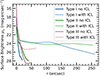 |
Fig. A.1. Surface brightness profiles μIE (in mag arcsec−2) for galaxies located at the minimum distance from the centre. The curves represent different types (Type I, Type II, and Type III) with or without the ICL component. |
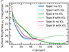 |
Fig. A.2. Surface brightness profiles μIE (in mag arcsec−2) for galaxies located at a median distance from the centre. The curves represent different types (Type I, Type II, and Type III) with or without the ICL component. |
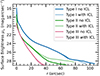 |
Fig. A.3. Surface brightness profiles μIE (in mag arcsec−2) for galaxies located at the maximum distance from the centre. The curves represent different types (Type I, Type II, and Type III) with or without the ICL component. |
Appendix B: Influence of the extended PSF on type profiles
We propose to investigate the impact of the extended PSF of Euclid’s cameras on the shapes of surface brightness profiles. As indicated in Cuillandre et al. (2025a), the fluxes are minimally affected by the extended PSF because it is very pure and extremely sharp. However, some recent studies, as Trujillo & Fliri (2016) and Borlaff et al. (2017), suggest that the shape of the disc profiles, specifically the positions of the breaks, can be significantly impacted by a poorly behaved extended PSF. Here, we aim to quantify this effect in the case of Euclid’s pristine extended PSF.
We begin our analysis with models of Type I, II, and III galaxies, using parameters corresponding to the median values measured in Tables 3 and 4. We then convolve this model with the extended PSF model provided in Cuillandre et al. (2025a). The results are presented in Fig. B.1.
We focus on the outer regions of the galaxies, i.e. beyond the sharp region of the PSF. In these cases, the PSF becomes influential only at a radius exceeding 40″for the three profiles. For Type II and III profiles, the corresponding area is beyond the down-bending disc break radius, which in median around 25″in the case of disc galaxies in the field. Therefore, the fitting parameters of the models vary by less than 4% between the original and convolved profiles. This justifies our decision not to account for the PSF in the profile fitting adjustments; specifically, we can say that the U-shaped colour profile is not simply due to the PSF influence.
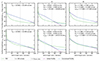 |
Fig. B.1. Influence of the extended PSF (IE on top and HE on bottom) on surface brightness profiles of Type I (right), Type II (middle), and Type III (left): the green line is the IE PSF (Cuillandre et al. 2025a); the purple lines give the initial profile which is pure simple exponential for Type I or double exponential for Type II; the blue lines correspond to the profile from the convolution of the initial profile and the PSF. |
Appendix C: Mean profile from AutoProf and AstroPhot
We present the distributions of normalised surface brightness profiles obtained using two extraction tools: AutoProf and AstroPhot. These profiles allow us to examine the variations in galaxy surface brightness as a function of the radius normalised by R25, while highlighting general trend. Each profile, originally consisting of approximately 20 points, has been resampled to 300 points using interpolation to ensure consistent representation and facilitate comparison across all profiles.
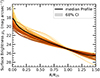 |
Fig. C.1. Distribution of normalised surface brightness profiles extracted with AutoProf. Individual profiles are displayed with a colour gradient, while the median profile is represented in black. The shaded region around the median indicates the 68% confidence interval, reflecting the variability among individual profiles. |
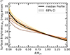 |
Fig. C.2. Distribution of normalised surface brightness profiles extracted with AstroPhot. Individual profiles are displayed with a colour gradient, while the median profile is represented in black. The shaded region around the median indicates the 68% confidence interval, reflecting the variability among individual profiles. |
Appendix D: Type profile
In this section, examples of the three types of surface brightness profiles are provided in Figs. D.1 to D.3. We display four panels for each type as follows:
Top Left Panel: Image of the galaxy with associated radii indicated by ellipses of different colours: green/yellow for the break positions in the surface brightness profiles of IE(μIE) and HE (μHE) bands, red for the radius at  , and blue for the boundary regions of interest in semi-major axis r where the break may potentially be found.
Top Right Panel: Surface brightness profile (μIE) versus axis ratio (r) of the fitted ellipses in the IE band. Solid lines indicate the fitted models: single Sérsic model in red, bulge/disc decomposition model in blue, bulge/disc1/disc2 decomposition model in green. Dashed lines indicate: blue for the boundary regions of interest in r where the break may potentially be found, green for the break position, red for the radius at  .
.
Bottom Right Panel: Surface brightness profile (μHE) versus axis ratio (r) of the fitted ellipses in the HE band. Solid lines indicate the fitted models after the radius of the bulge: disc model in blue, disc1/disc2 model in green. Dashed lines indicate the boundary regions of interest in r where the break may potentially be found in blue and the break position in yellow.
Bottom Left Panel: Magnitude difference (IE− HE) as a function of r in the blue region of interest.
In Fig. D.1, the top right panel shows that the single Sérsic model – red line – gives a low Sérsic index and does not fit the data well beyond a certain radius. Its chi-square value is higher compared to the other two models. It is observed that the disc models provide a better fit, with the double disc model indicating a very late break around a surface brightness of 28, which does not correspond to a typical Type II or Type III profile.
In contrast, Fig. D.2 clearly shows a down-bending disc break near a magnitude of 25. The double disc model in green gives the best chi-square value.
Finally, in Fig. D.3, a Type III profile is clearly identified by the up-bending exponential profile model.
It can also be noted that the bottom left panels, showing the magnitude variation between the IE and HE bands, indicate no gradient for any of these examples, particularly after the break for Type II and III profiles.
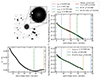 |
Fig. D.1. Profile of the galaxy WISEA J031851_10+412332_5 – Type I |
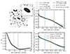 |
Fig. D.2. Profile of the galaxy UGC 02665 – Type II |
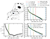 |
Fig. D.3. Profile of the galaxy WISEA J032042_17+412414_2 – Type III |
Appendix E: Characterisation of the morphological classification
This appendix is dedicated to the validation of the morphological classification by verifying several aspects. In addition to comparisons for a large portion of the galaxies, approximately 60, to the literature, we also perform measurements of the bulge luminosity and the bulge-to-total light ratio for the morphological types S0 (type −1), intermediate between S0 and pure spirals (type 0), and spiral galaxies (type 1). These metrics are widely used in the literature to classify the morphologies of disc galaxies through the characterisation of their bulge (Quilley & de Lapparent 2023).
In Fig. E.1, the grey points represent these measurements for each disc galaxy according to its morphological class. The mean and standard deviation for each value are also provided. Clearly, as expected, the average surface brightness of the bulges increases with the evolutionary stage of the disc galaxies. Similarly, the right panel shows a slight decrease with the bulge flux fraction from S0 to spiral galaxies. Overall, our classification is validated by these results.
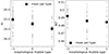 |
Fig. E.1. Validation of morphological classifications. Left Panel: Bulge surface brightness measurements for disc galaxies according to morphological classes (S0, intermediate, spirals). Grey points represent individual measurements, while the dark squares give the mean and standard deviation of each distribution. Right Panel: Bulge-to-total light ratio as a function of morphological type. |
Appendix F: Fitted parameters
Figure F.1 presents the distribution of fitted parameters obtained using the double exponential profile in the IE band for Type II (down-bending break) and Type III (up-bending break) profiles. The disc scalelengths and down-bending break radii are compared to the effective radii provided in the catalogue from Cuillandre et al. (2025b). It is observed that the break occurs well beyond the effective radius of the galaxy, as shown in the rightmost panel. The scalelengths of the first disc are of the order of the galaxy’s effective radius. One of the up-bending break galaxies has a value significantly higher than this effective radius, but no significant issue in the fit was found. For the scalelength of the second disc, as expected, values significantly lower than the effective radius are found for Type II profiles, while higher values are found for Type III profiles.
In Fig. F.2, the distribution of disc scalelengths and break radii from fits in the HE band are compared with those in the IE band. The solid line represents the identity line to facilitate comparison between the two bands. The parameters are consistent across both bands, with a slight tendency for the scalelength of the first disc to be shorter in the infrared than in the visible, a trend noted in Laine et al. (2016).
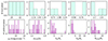 |
Fig. F.1. Distribution of fitting parameters using the double exponential profile in the IE band for Type II (down-bending break in higher panels) and Type III (up-bending break in lower panels) profiles. The scalelengths of the discs and down-bending break radii are compared to the effective radii from the main Perseus catalogue Cuillandre et al. (2025b). First panel: Distribution of the central surface brightness of the discs. Second panel: Distribution of the break surface brightness compared to the central surface brightness of the discs. Third panel: Distribution of first disc scalelengths. Fourth panel: Distribution of second disc scalelengths. Fifth panel: Break radii compared to the effective radius of the galaxy. |
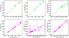 |
Fig. F.2. Distribution of disc scalelengths and break radii for Type II (higher panels) and for Type III (lower panels) in the HE band as a function of those in the IE band. The solid line represents the identity line for comparison between the two bands. |
All Tables
Parameters of the double exponential model for the four identified down-bending disc breaks (Type II) in our sample.
Parameters of the double exponential model for the 24 identified up-bending disc breaks (Type III) in our sample.
All Figures
|
Fig. 1. IE image of the Perseus field of view after subtraction of the intra-cluster light (ICL): blue dots indicate the position of each disc galaxy, red dots show the position of ellipticals. Orange lines shows the right ascension and the declination of IE image. In the background, the method of identification for each galaxy is displayed, with visual markers distinguishing galaxies classified by photometric redshifts (zphot, square symbols) and spectroscopic redshifts (zspec, circular symbols). The yellow dot highlights the location of the cluster centre (NGC 1275). |
| In the text | |
|
Fig. 2. Scaling relations between the Sérsic index n, the effective radius Re, the central surface brightness μ0, mean effective surface brightness within Re, ⟨μe⟩, the mass log10(M*/M⊙) and the total magnitude IE of galaxies measured using AutoProf/AstroPhot. The blue distribution shows the probability density function for the 102 cluster member bright disc galaxies while red dots are for cluster member bright ellipticals. The surface brightness is given in mag arcsec−2. The panels on the top and side provide the normalised histograms of the parameters for discs (in blue) and for ellipticals (in red). |
| In the text | |
|
Fig. 3. Examples of different types of interactions observed in the Perseus cluster. Each panel shows a LSB IE image with high contrast of a galactic interaction within the cluster. A red line in the bottom-right corner representing a scale of 10″ is provided at the bottom of each panel. Top left: NGC 1268 – a galaxy with a smooth, elongated shape, likely experiencing a close encounter with a neighbouring galaxy, causing mild distortion in its outer regions. Top centre: NGC 1282 – an interacting galaxy with a faint halo, possibly stripped due to gravitational forces from nearby massive galaxies. Top right: GALEXASC J031939.68+413105.6 – a disrupted galaxy showing two tidal rings, suggesting a recent interaction or minor merger with another galaxy. Middle left: PGC 012221 – a galaxy with a clear spiral structure that appears distorted, possibly due to tidal forces. Middle centre: PGC 012358 – a major merger with an asymmetrical shape and tidal tails, showing evidence of material being pulled away. Middle right: PGC 012520 – an elongated galaxy with an asymmetric stretched halo, suggesting ongoing gravitational interactions or stripping by the cluster’s dense environment. Bottom left/centre: MCG+07-07-070 and UGC 02665 – galaxies possibly affected by ram pressure stripping due to their motion through the intracluster medium. MCG+07-07-070 shows an asymmetric diffuse halo extending towards the lower right, while UGC 02665 displays an umbrella-like morphology, both consistent with ram-pressure stripping (George et al. in prep.). Bottom right: WISEA J032020.96+41225.4 – a galaxy interacting with a larger galaxy, showing faint tidal features, which may indicate gravitational influence from a nearby massive galaxy. |
| In the text | |
|
Fig. 4. Star masking process. Left: image of a 2 k × 2 k tile (i.e. 3 |
| In the text | |
|
Fig. 5. Several steps of the AutoProf process for WISEA J031817.90+414031.0 for a IE (top) and a HE (bottom) images. Left: Initialisation of the first ellipse in cyan around the central galaxy. Middle: Final isophote fitting. Using red and cyan colours enhances the visualisation and counting of isophotes (Stone et al. 2021) Right: Extraction of the radial surface brightness profile. Note that cyan points are drawn each four isophotes. |
| In the text | |
|
Fig. 6. Steps of the AstroPhot process for NGC 1260 and its neighbouring galaxies for a IE image. Top left: Detection of stars (in yellow) from the SExtractor segmentation map. Top right: Masking of stars on the 4 k × 4 k image centred on NGC 1260. Bottom left: Final fitting of galaxies provided by AstroPhot, colour coded by the surface brightness value. Bottom right: Final residual map. |
| In the text | |
|
Fig. 7. Residual image in the IE field of the Perseus cluster (after ICL subtracting): The centres of elliptical (E) galaxies are marked with red dots, S0 galaxies with green dots, intermediate types between S0 and spirals with cyan dots, and spirals with dark blue dots. Coloured circles, centred on the central elliptical galaxy NGC 1275, indicate the average projected distance for each morphological type. |
| In the text | |
|
Fig. 8. Distribution of normalised surface brightness profiles for different types of galaxies. The subplots show the profiles for Type II (top left), Type III (top right), Type I (bottom left), and the combined median profiles for the three types around R = Rnorm (bottom right). Individual profiles are displayed with a colour gradient, while the median profile is represented in black. The shaded region around the median indicates the 68% confidence interval, reflecting the variability among individual profiles. Note that Rnorm corresponds to R25 for Type I or Rbreak for Type II and III. |
| In the text | |
|
Fig. 9. Ratio of the truncation radius to the first disc scalelength (Rbreak/hd1) as a function of the logarithm of the ratio between the disc scalelengths (hd1/hd2). This plot visually separates Type II galaxies (green dots) from Type III galaxies (magenta dots). The error bars are directly extracted from the uncertainties on the parameters obtained during the surface brightness profile fitting process. |
| In the text | |
|
Fig. 10. Kernel density estimation plot of the distribution of the complete catalogue (dwarfs + bright galaxies) in the right ascension versus declination plane: four probability density bins are indicated in colour, showing higher probability density in the centre in red and lower density in the outskirts in pale yellow. Dots are overplotted on this distribution to indicate the positions of Type II galaxies in green and Type III galaxies in magenta. The black cross indicates the centre of NGC 1275. |
| In the text | |
|
Fig. 11. Fraction of each type within the total population of spiral to S0 galaxies: Type I, Type II and Type III. The grey bars indicate the total fraction of each type. The coloured bars, ranging from dark red to pale yellow, show the fraction of each type within each region from the core to the outer regions. Error bars represent the 1σ binomial uncertainties calculated as |
| In the text | |
|
Fig. 12. Fraction of galaxies in each density bin for each Type profiles for the different Hubble morphological type: one corresponds to spirals (darkblue), zero to S0/spiral intermediates (cyan), and minus one to confirmed S0 galaxies (green). Error bars represent the 1σ binomial uncertainties calculated as |
| In the text | |
|
Fig. 13. Fraction of each profile type (I, II, III) according to the angular projection within the cluster (from red to yellow) similar to Fig. 11 but for different galaxy morphology from Hubble type −1 on the left-hand panel, to one on the right-hand panel. Error bars represent the 1σ binomial uncertainties calculated as |
| In the text | |
|
Fig. 14. Stellar mass distribution of galaxies according to their position in the cluster. Left-hand panel: stellar mass distribution of galaxies across the different environments (from outskirts – top left panel – to core – bottom right panel), each represented by a different colour as labelled. Right-hand panel: galaxy mass as a function of probability density, with individual galaxies represented by grey dots. The black curve indicates the rolling average over 10 galaxies, black squares show the mean, and green dots represent the median for each density bin. The error bars corresponds to the standard error on the mean and median. |
| In the text | |
|
Fig. 15. The fraction of each profile type (I, II, III) according to the angular projection within the cluster (from red to yellow) similar to Fig. 11 but for three different stellar mass bins from left/lower masses to right/larger masses as labelled. Error bars represent the 1σ binomial uncertainties calculated as |
| In the text | |
|
Fig. 16. Normalised magnitude difference IE− HE as a function of radius R/Rbreak for galaxies Type II, Type III and Type III with a detected U-shaped profile. The profiles are normalised around R = Rbreak. The minimum value within the range 0.5 ≤ R/Rbreak ≤ 1.5 is identified. |
| In the text | |
|
Fig. 17. Profile of the galaxy SDSS 1237661122387969061. Top Left Panel: Image of the galaxy with associated radii indicated by ellipses of different colours: green/yellow for the break positions in the surface brightness profiles of IE (μIE) and HE (μHE) bands, red for the radius at |
| In the text | |
|
Fig. 18. Hydrodynamical simulations of the interaction of a Type II galaxy with a Perseus-like cluster. The initial disc galaxy (solid black curve) has a double exponential, Type II radial profile, and a central bulge, formed by disc instabilities at high redshift, with a break at 6.5 kpc and a gas fraction of 17% in the disc. These initial conditions are taken from simulations of high-redshift disc instabilities and Type II profile formation in Bournaud et al. (2007). Simulations (Paper II) evolve this disc galaxy in the tidal field of the Perseus-like cluster for about one cluster crossing time. The median profile over six simulated orbits (red dashed curve) and the RMS dispersion (shaded area) are displayed, showing that the galaxy evolves most of the time towards a Type I disc, while the same galaxy in isolation during the same timescale would remain Type II (thin blue line with diamonds). Stars pre-existing to the galaxy/cluster interaction (red dotted line) are scattered radially over increasingly eccentric orbit, accounting for about two thirds of the replenishment of the outer disc beyond the initial break radius, the other third coming from the triggering of turbulence, shocks, and star formation in the outer disc by the tidal field of the cluster (see Paper II for individual orbits and detailed interpretation). |
| In the text | |
|
Fig. 19. IE LSB images of four down-bending break galaxies. The truncation is indicated by the green dashed ellipse, i.e the isophote with a semi-major axis equal to that of the break. The outer region lies beyond this isophote. The red ellipse denotes the radius at μIE = 25 mag arcsec−2. We note that the red circle is close to the green circle. The line at the bottom right of each image gives the scale, which corresponds to 10″. |
| In the text | |
|
Fig. 20. IE LSB images of up-bending break galaxies. The break is indicated by the green dashed ellipse, i.e the isophote with a semi-major axis equal to that of the break. The red ellipse denotes the radius at μIE = 25 mag arcsec−2. We note that the red circle is close to the green circle, in most of the cases. The line at the bottom right of each image gives the scale, which corresponds to 10″. |
| In the text | |
|
Fig. A.1. Surface brightness profiles μIE (in mag arcsec−2) for galaxies located at the minimum distance from the centre. The curves represent different types (Type I, Type II, and Type III) with or without the ICL component. |
| In the text | |
|
Fig. A.2. Surface brightness profiles μIE (in mag arcsec−2) for galaxies located at a median distance from the centre. The curves represent different types (Type I, Type II, and Type III) with or without the ICL component. |
| In the text | |
|
Fig. A.3. Surface brightness profiles μIE (in mag arcsec−2) for galaxies located at the maximum distance from the centre. The curves represent different types (Type I, Type II, and Type III) with or without the ICL component. |
| In the text | |
|
Fig. B.1. Influence of the extended PSF (IE on top and HE on bottom) on surface brightness profiles of Type I (right), Type II (middle), and Type III (left): the green line is the IE PSF (Cuillandre et al. 2025a); the purple lines give the initial profile which is pure simple exponential for Type I or double exponential for Type II; the blue lines correspond to the profile from the convolution of the initial profile and the PSF. |
| In the text | |
|
Fig. C.1. Distribution of normalised surface brightness profiles extracted with AutoProf. Individual profiles are displayed with a colour gradient, while the median profile is represented in black. The shaded region around the median indicates the 68% confidence interval, reflecting the variability among individual profiles. |
| In the text | |
|
Fig. C.2. Distribution of normalised surface brightness profiles extracted with AstroPhot. Individual profiles are displayed with a colour gradient, while the median profile is represented in black. The shaded region around the median indicates the 68% confidence interval, reflecting the variability among individual profiles. |
| In the text | |
|
Fig. D.1. Profile of the galaxy WISEA J031851_10+412332_5 – Type I |
| In the text | |
|
Fig. D.2. Profile of the galaxy UGC 02665 – Type II |
| In the text | |
|
Fig. D.3. Profile of the galaxy WISEA J032042_17+412414_2 – Type III |
| In the text | |
|
Fig. E.1. Validation of morphological classifications. Left Panel: Bulge surface brightness measurements for disc galaxies according to morphological classes (S0, intermediate, spirals). Grey points represent individual measurements, while the dark squares give the mean and standard deviation of each distribution. Right Panel: Bulge-to-total light ratio as a function of morphological type. |
| In the text | |
|
Fig. F.1. Distribution of fitting parameters using the double exponential profile in the IE band for Type II (down-bending break in higher panels) and Type III (up-bending break in lower panels) profiles. The scalelengths of the discs and down-bending break radii are compared to the effective radii from the main Perseus catalogue Cuillandre et al. (2025b). First panel: Distribution of the central surface brightness of the discs. Second panel: Distribution of the break surface brightness compared to the central surface brightness of the discs. Third panel: Distribution of first disc scalelengths. Fourth panel: Distribution of second disc scalelengths. Fifth panel: Break radii compared to the effective radius of the galaxy. |
| In the text | |
|
Fig. F.2. Distribution of disc scalelengths and break radii for Type II (higher panels) and for Type III (lower panels) in the HE band as a function of those in the IE band. The solid line represents the identity line for comparison between the two bands. |
| In the text | |
Current usage metrics show cumulative count of Article Views (full-text article views including HTML views, PDF and ePub downloads, according to the available data) and Abstracts Views on Vision4Press platform.
Data correspond to usage on the plateform after 2015. The current usage metrics is available 48-96 hours after online publication and is updated daily on week days.
Initial download of the metrics may take a while.