| Issue |
A&A
Volume 677, September 2023
|
|
|---|---|---|
| Article Number | A117 | |
| Number of page(s) | 20 | |
| Section | Extragalactic astronomy | |
| DOI | https://doi.org/10.1051/0004-6361/202346719 | |
| Published online | 14 September 2023 | |
The AMIGA sample of isolated galaxies
XIV. Disc breaks and interactions through ultra-deep optical imaging⋆
1
Instituto de Astrofísica de Canarias, c/ Vía Láctea s/n, 38205 La Laguna, Tenerife, Spain
e-mail: This email address is being protected from spambots. You need JavaScript enabled to view it.
2
Departamento de Astrofísica, Universidad de La Laguna, 38206 La Laguna, Tenerife, Spain
e-mail: This email address is being protected from spambots. You need JavaScript enabled to view it.
3
Instituto de Astrofísica de Andalucía (CSIC), Granada, Spain
4
Kapteyn Astronomical Institute, University of Groningen, PO Box 800 9700 AV Groningen, The Netherlands
5
Department of Physics & Astronomy, University of California Los Angeles, 430 Portola Plaza, Los Angeles, CA 90095-1547, USA
6
Departamento de Física Teórica y del Cosmos Universidad de Granada, 18071 Granada, Spain
7
Instituto Universitario Carlos I de Física Teórica y Computacional, Universidad de Granada, 18071 Granada, Spain
8
ESA NEO Coordination Centre, Via Galileo Galilei, 00044 Frascati (RM), Italy
9
GMV, Isaac Newton 11, Tres Cantos, 28760 Madrid, Spain
10
Centro de Astronomía (CITEVA), Universidad de Antofagasta, Avda. U. de Antofagasta 02800, Antofagasta, Chile
Received:
20
April
2023
Accepted:
29
June
2023
Abstract
Context. In the standard cosmological model of galaxy evolution, mergers and interactions play a fundamental role in shaping galaxies. Galaxies that are currently isolated are thus interesting because they allow us to distinguish between internal and external processes that affect the galactic structure. However, current observational limits may obscure crucial information in the low-mass or low-brightness regime.
Aims. We use optical imaging of a subsample of the AMIGA catalogue of isolated galaxies to explore the impact of different factors on the structure of these galaxies. In particular, we study the type of disc break as a function of the degree of isolation and the presence of interaction indicators such as tidal streams or plumes, which are only detectable in the ultra-low surface brightness regime.
Methods. We present ultra-deep optical imaging in the r band of a sample of 25 low-redshift (z < 0.035) isolated galaxies. Through careful data processing and analysis techniques, the nominal surface brightness limits achieved are comparable to those to be obtained on the ten-year LSST coadds (μr,lim ≳ 29.5 mag arcsec−2 [3σ; 10″ × 10″]). We place special emphasis on preserving the low surface brightness features throughout the processing.
Results. The extreme depth of our imaging allows us to study the interaction signatures of 20 galaxies since Galactic cirrus is a strong limiting factor in the characterisation of interactions for the remaining 5 of them. We detect previously unreported interaction features in 8 (40% ± 14%) galaxies in our sample. We identify 9 galaxies (36% ± 10%) with an exponential disc (Type I), 14 galaxies (56% ± 10%) with a down-bending (Type II) profile, and only 2 galaxies (8% ± 5%) with up-bending (Type III) profiles. Isolated galaxies have considerably more purely exponential discs and fewer up-bending surface brightness profiles than field or cluster galaxies. We find clear minor merger activity in some of the galaxies with single exponential or down-bending profiles, and both of the galaxies with up-bending profiles show signatures of a past interaction.
Conclusions. We show the importance of ultra-deep optical imaging in revealing faint external features in galaxies that indicate a probable history of interaction. We confirm that up-bending profiles are likely produced by major mergers, while down-bending profiles are probably formed by a threshold in star formation. Unperturbed galaxies that slowly evolve with a low star formation rate could induce the high rate of Type I discs in isolated galaxies.
Key words: galaxies: evolution / galaxies: structure / galaxies: photometry / galaxies: interactions
All the images, masks, and profile tables are only available at the CDS via anonymous ftp to cdsarc.cds.unistra.fr (130.79.128.5) or via https://cdsarc.cds.unistra.fr/viz-bin/cat/J/A+A/677/A117
© The Authors 2023
 Open Access article, published by EDP Sciences, under the terms of the Creative Commons Attribution License (https://creativecommons.org/licenses/by/4.0), which permits unrestricted use, distribution, and reproduction in any medium, provided the original work is properly cited.
This article is published in open access under the Subscribe to Open model. This email address is being protected from spambots. You need JavaScript enabled to view it. to support open access publication.
1. Introduction
Present-day galactic discs are snapshots of the galaxy evolution that resulted from galaxy formation and evolution through cosmic time. The study of galaxies with a variety of morphologies, evolutionary stages, and environments helps us to assemble a global picture to explain all the observed features. One of the simplest but most effective ways to classify galactic structures is through their surface brightness profiles. These profiles were initially characterised with a single exponential decay by Patterson (1940) and de Vaucouleurs (1958), but the current view is considerably more complex. Following the observation of breaks in profiles by van der Kruit (1979) and van der Kruit & Searle (1981a,b) at the outer regions of the edge-on galaxies, Erwin et al. (2005) and Pohlen & Trujillo (2006) considered breaks over a range of galactocentric radii and in less-inclined galaxies. These authors established a classification based on the global shape of the disk profile: Type I or pure exponential for profiles with no breaks, Type II or down-bending profiles in which the outer slopes are steeper than the inner ones (e.g., Freeman 1970; Pohlen et al. 2002), and Type III or up-bending profiles in which the exponential decline is steeper in the inner part of the disc than in the outer part (e.g., Erwin et al. 2005). This classification has been helpful because galaxies have different average properties for each type, which suggests a different origin or evolution.
One of the most characteristic features in discs is the drastic change in age around the break radius, which is noticed as a U-shape in the colour profiles, while the mass surface density profile remains relatively constant (e.g., Azzollini et al. 2008; Bakos et al. 2008; Bakos & Trujillo 2012; Martín-Navarro et al. 2012; Zheng et al. 2015; Watkins et al. 2016; Ruiz-Lara et al. 2016). This observational feature has been tentatively explained as the result of gas accretion plus a density threshold in the star formation and a subsequent redistribution of mass by radial migration (e.g., Debattista et al. 2006; Roškar et al. 2008; Martínez-Serrano et al. 2009), which has been described as inside-out formation of the disc (Sánchez-Blázquez et al. 2009).
The environment appears to play a key role in the frequency of each break type (e.g., Pranger et al. 2017; Watkins et al. 2019). In general, high-density environments favour up-bending Type III profiles (see Maltby et al. 2012). This is expected because the environment is one of the most influential factors in shaping galactic morphology (e.g., Balogh et al. 2004; Thomas et al. 2005; Baldry et al. 2006; Erwin et al. 2012). However, internal processes (e.g., Kormendy & Kennicutt 2004) or the accretion of cold gas (Bosma 2017) are also capable of transforming the galaxy characteristics. Correlations between the type of break (in particular, the Type III fraction) with internal parameters (Herpich et al. 2017; Wang et al. 2018) and possible interactions (Eliche-Moral et al. 2015; Borlaff et al. 2018) are also found. Adding more complexity, instrumental effects including background subtraction or scattered light can have a significant effect on the photometric profiles, especially at extremely low surface brightness (Sandin 2014). This means that determining the specific impact of different processes is not a straightforward task. A possible approach is studying isolated galaxies to exclude or diminish the impact of environmental processes (e.g., Karachentseva 1973; Huchra & Thuan 1977; Arakelian & Magtesian 1981; Schwarzkopf & Dettmar 2001; Varela et al. 2004).
Determining and quantifying the isolation of a galaxy is not a simple task. The project called Analysis of the interstellar Medium of Isolated GAlaxies (AMIGA; Verdes-Montenegro et al. 2005) is an exhaustive study of galaxies that are isolated from main companions. It is based on the original catalogue of isolated galaxies (CIG) presented by Karachentseva (1973) and later revised and quantified by Verley et al. (2007a,b) and Argudo-Fernández et al. (2013). Despite the efforts shown in these works to quantify minor interaction features, spectroscopic and imaging surveys with a low signal-to-noise ratio may fail to identify faint surface brightness satellites around galaxies that are classified as isolated. Numerical simulations based on the Λ-CDM cosmological paradigm predict an average of one low surface brightness feature per galaxy due to minor interactions at a surface brightness level of μ = 29 mag arcsec−2 (Johnston et al. 2001), and we can expect many galaxy features fainter than μ = 30 mag arcsec−2 (Johnston et al. 2008).
The interest in low surface brightness science is confronted with significant challenges due to numerous observational limitations. Advances have been made in recent years in developing deep optical surveys (e.g., Laine et al. 2014; Abraham & van Dokkum 2014; Fliri & Trujillo 2016; Dark Energy Survey Collaboration 2016; Román & Trujillo 2018; Aihara et al. 2018; Martínez-Delgado 2019; Trujillo et al. 2021), characterising scattered light (e.g., Slater et al. 2009; Karabal et al. 2017; Infante-Sainz et al. 2020), improving observational (Jablonka et al. 2010; Duc et al. 2015; Mihos et al. 2017; Trujillo & Fliri 2016; Staudaher et al. 2019) and data-processing techniques (Jiang et al. 2014; Trujillo & Fliri 2016; Borlaff et al. 2019; Haigh et al. 2021), and more (see review by Mihos 2019). Increasingly sophisticated studies are able to reveal the presence of satellites (Laine et al. 2014; Mihos et al. 2015; Román et al. 2021) and tidal features (Laine et al. 2014; Martínez-Delgado 2019; Martínez-Delgado et al. 2023; Huang & Fan 2022; Román et al. 2023) at increasingly lower surface brightness, but correctly detecting and classifying all the structures predicted by simulations is still a work in progress (see Martin et al. 2022, and references therein).
In this work, we carry out an ultra-deep imaging study of isolated galaxies from the AMIGA catalogue in order to shed light on the structural differences between these isolated galaxies and galaxies in higher-density environments. In particular, we are interested in 1) the types of breaks in the discs of isolated galaxies in comparison with those in higher-density environments. This has not yet been done in the literature for isolated galaxies, and has only been carried out so far by comparing higher-density environments such as clusters, and groups with simply the “field”. 2) We are also interested in using low surface brightness imaging to explore minor interactions in these isolated galaxies. 3) Finally, we explore possible correlations between the type of break, minor interactions, and density, which can help elucidate the dominant factors that shape the galaxy discs.
This work is structured as follows: In Sect. 2 we describe the data sample and the reduction procedure we followed. In Sect. 3 we explain the methods we used to measure the surface brightness profiles, classify the profiles by type, and detect signs of interaction. In Sect. 4 we present the results, which are discussed in Sect. 5. The conclusions of our work are summarised in Sect. 6. We adopt the values of the cosmological constants H0 = 70 km s−1 Mpc−1, T0 = 2.725 K, and Ωm = 0.3. Galactic extinction is corrected following Schlafly & Finkbeiner (2011). We use the AB photometric system.
2. Sample, data, and processing
2.1. Sample selection and observations
We used the AMIGA sample (Verdes-Montenegro et al. 2005), which is based on the original CIG catalogue by Karachentseva (1973). The latest revision of the isolation parameters of the AMIGA catalogue was carried out by Argudo-Fernández et al. (2013). We base the selection of our sample on this work.
Our selection criteria were as follows. The targets were to be part of the AMIGA catalogue. We required that the galaxies had a reliable determination of the distance (latest revision for AMIGA sample in Jones et al. 2018) as well as a detection in H I, in order to also further explore possible correlations between the fainter optical morphology and their gas content. The photometric isolation parameters measured by Verley et al. (2007b) are the local number density of neighbour galaxies, ηk, p, and the tidal strength, QKar, p. We required galaxies to have a local number density of neighbouring galaxies ηk, p < 2.7.
We observed 25 galaxies meeting these criteria with different telescopes. The morphologies of these galaxies range from Hubble types of 3 ≤ T ≤ 5, which is a similar sample as in the complete AMIGA catalogue (see Sulentic et al. 2006). Here we briefly describe the instrumentation we used. 1) The Isaac Newton Telescope (INT), located in the Observatorio del Roque de los Muchachos in La Palma, Spain, has a 2.5 m diameter primary mirror. We used the Wide Field Camera (WFC), a four-CCD mosaic covering 33 arcmin on a side, with a pixel scale of 0 333. 2) The VLT Survey Telescope (VST), located in Cerro Paranal, Chile. The VST has a 2.65 m primary mirror. We used OmegaCAM, which has 32 CCDs covering a field of view (FOV) of approximately 1 degree2, with a pixel scale of 0
 21. 3) The 0.7 m Jeanne-Rich Telescope (JRT) is located at the Polaris Observatory Association site, Pine Mountain, California. The camera covers approximately 40 arcmin on a side, with a pixel scale of 1
 114.
114.
Due to the high observational cost of ultra-deep optical imaging and to optimise the detection of faint features, we only obtained r-band data. Observations were mostly carried out in dark time, although grey nights with little Moon were also used. In the worst cases, the Moon was far enough with a low phase to not produce any gradient in the image. Dithering patterns of tens of arcseconds were used in order to improve the flat field. The exposure time was set between one and five minutes for each individual frame.
The imposed surface brightness limits rule out the use of most general-purpose optical surveys. Only the Hyper Suprime-Cam Subaru Strategic Program (HSC-SSP; Aihara et al. 2018) was able to fulfil our surface brightness requirements. HSC-SSP is a survey produced with the Subaru 8.2 m aperture telescope and the Hyper Suprime-Cam. We found four galaxies within the HSC-SSP footprint meeting our selection criteria. These are included in our sample. We used the second data release of the survey (Aihara et al. 2019). Although there are additional filters, we only used the r-band data for the purposes of our work.
We set a requirement of μr,lim > 29.5 mag arcsec−2 for the surface brightness measured as 3σ in 10″ × 10″ boxes following the nominal depth description by Román et al. (2020). This limit was set as a compromise between deep images to detect faint structures and observational costs. We added an exception to this limit to data from the JRT. This telescope has a small aperture, but is built to be extremely efficient in the low surface brightness regime. Therefore, although the Poissonian noise with which the surface brightness limits are measured will tend to be higher for this telescope, the detectability of extremely low surface brightness features is comparable to data of higher nominal depth, as we show in the results section. Additionally, on this telescope, we used a broad luminance band in order to maximise detection. This type of band has been proven to be similar to the r band (Martínez-Delgado et al. 2015). We therefore set a limit of μL,lim > 28.5 mag arcsec−2 for data from the JRT.
2.2. Data reduction
The observations were reduced following a procedure aimed at preserving the low surface brightness features. First, a bias subtraction (and dark, if necessary) was performed, following an ordinary procedure of combining bias images (and dark). For the flat-fielding, we used the science images themselves. This procedure consists of using heavily masked science images, masked with specialised software such as SExtractor (Bertin & Arnouts 1996, version 2.25.0) and Noisechisel (Akhlaghi & Ichikawa 2015, version 0.18), which are normalised in flux and subsequently combined using a resistant mean algorithm to produce a flat that is representative of the sky background during the observations. This procedure, building the flat from the science images, has significant advantages over the usual dome or twilight flats. The main advantage is a considerable decrease in the strength of gradients in the images, allowing, as we detail below, a less aggressive subtraction of the sky background, and therefore a higher reliability of the characterisation of the faintest sources. An additional advantage is that the fringing structures contained in the science images are perfectly corrected, allowing us to improve the quality of the final images. Because the sensitivity of the CCD cameras can vary over time and the time range between different observations is very wide (of the order of years), the flats are built and applied to data sets taken close in time, typically during the few days of each observation campaign.
After the images were reduced, we proceeded to combine them. First, the images were astrometrically calibrated, using the Astrometry.net software package (Lang et al. 2010) to obtain an approximate solution, and SCAMP (Bertin 2006) to obtain the final astrometry. The next step was the coaddition of the individual frames, which is the most crucial step in the process. We performed an iterative loop converging on what we consider the final coadd. The procedure was as follows. First, we obtained a seed coadd, which is the starting point of the iteration. This coadd was produced by subtracting a constant sky value for each of the individual frames to be combined. The consequence of this is that we preserved the lowest surface brightness structures that were not removed by the sky subtraction. However, the frequent gradients in the individual frames produce considerable fluctuations in the sky background, which remain in the coadd. This coadd was heavily masked with Noisechisel, choosing parameters that maximised the masking of the real sources, trying to leave the smooth gradients of the sky background unmasked. This mask produced with the coadd was applied to the individual frames, and we performed a smooth polynomial sky fitting to the individual masked frames. We used Zernike polynomials (see Zernike 1934) as sky-fitting surfaces, always with values equal to or lower than n≤ 4, using for each n order all the azimuthal components. This Zernike polynomial fitting produced smooth surfaces that did not impact in the oversubstraction around galaxies. After all the gradients of the individual frames were fitted and subtracted, they were combined to produce a new coadd that was used again as a seed to obtain a new mask. This process was iterated a number of times. Depending on how strong the gradients were, the number of iterations and the degree of the polynomial were varied to obtain an optimal result. In most cases, the polynomials have a low degree (n = 2, 3) because of the high quality of flat-fielding. In extreme cases, and mainly due to the presence of the Moon in the observations, we increased the degree of the polynomial (n = 4) in order to obtain an optimal final coadd. In general, the reliability of our sky background subtraction allowed us to preserve the lower surface brightness structures within our depth limits. We did not find signs of oversubtraction in the images and profiles, such as high-contrast regions close to the end of the galaxies or systematically truncated profiles (see Sect. 3.3). The combination process was performed by photometrically calibrating the individual frames, measuring their signal-to-noise ratio, and combining them by means of a weighted mean, thus optimising the signal-to-noise ratio of the final coadd.
In Table 1 we show the final sample. The depth of the images was calculated following the method of Román et al. (2020), Appendix A, according to a standard metric of 3 sigma in 10″ × 10″ boxes. All galaxies have a nominal limiting surface brightness above 29.5 mag arcsec−2, except for those observed with the JRT, which, as already mentioned, have a slightly lower nominal depth. This is compensated for by their flatter fields on large angular scales. The total integration time of our campaign, excluding data from the HSC-SSP survey, was 110 hours.
Observational and physical properties of the 25 galaxies.
In Fig. 1 we show the galaxy CIG 340 together with a comparison with SDSS (Abazajian et al. 2009) and Legacy Survey data (Dark Energy Survey Collaboration 2016). The difference in depth is significant between the data obtained in our work (30.3 mag arcsec−2), SDSS (27.6 mag arcsec−2) and the Legacy Survey (28.8 mag arcsec−2), all measured at [3σ; 10″ × 10″]. While the morphology of CIG 340 appears to be similar in the SDSS and the Legacy Survey, we detect new structure in our data, with a clear tidal stream south of CIG 340 and diffuse light appearing in the direction transverse to the disc, showing a halo-like structure. This highlights the considerable jump in detection power from previously existing data and the capacity of our observations to reveal past minor interactions.
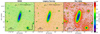 |
Fig. 1. r-band images of the galaxy CIG 340 (IC 2487) from different surveys. Comparison between the Sloan Digital Sky Survey (left), the Legacy Survey (middle), and our data. The upper right value indicates the surface brightness limit [3σ, 10″ × 10″] of each image computed as explained in Sect. 2. The arrow in the left panel indicates the low surface brightness feature that is only visible in our data. |
3. Analysis
3.1. Masking procedure
The masking of light coming from sources other than the target galaxy is one of the most delicate processes needed to obtain the cleanest and deepest possible surface brightness profiles. This task not only requires extracting the signal of astronomical sources from the emission of the background, but also requires the attribution (segmentation and deblending) of the signal to one particular source when there is an overlap.
We combined two of the most popular software tools used in astronomical detection, SExtractor (Bertin & Arnouts 1996, version 2.25.0) and NoiseChisel and Segment (Akhlaghi 2019, version 0.18), which are part of the GNUastro package. First, we ran NoiseChisel & Segment in hot and cold configuration modes for the whole set of images. This allowed us to select a region occupied by the galaxy of interest. Because this algorithm can detect very low signal-to-noise ratios (lower than ≲1), this region extends to very low surface brightness (≲27 mag arcsec−2), including the outskirts of the galaxy. We executed SExtractor with the parameters set to optimise the detection of point-like sources (the configuration file can be found in Appendix A). All the sources detected outside the galaxy region were then masked.
To improve the detection of the faintest parts of the sources, we first smoothed the image with the fully adaptive Bayesian algorithm for data analysis, FABADA (Sánchez-Alarcón & Ascasibar 2023, version 0.1). We used an overestimation of the variance of the image in FABADA to obtain a slightly smoother result and thus larger masks. This allows the detection of even fainter point sources in the proximity of the outskirts of galaxy.
Because we did not mask smaller sources inside the large region occupied by the galaxy, we ran an additional step to mask these objects. We masked all the sources detected by SExtractor outside a smaller region occupied by the galaxy, which corresponds to a level of five times the standard deviation of the image. NoiseChisel was then run again on the image with the mask applied. This last step allowed the detection of faint extended regions in the image. Because of the depth of our data, a considerable number of faint extended regions (e.g., stellar haloes of background sources, Galactic cirrus, reflections from bright stars, and residual light) appear in the images. All regions that were not spatially connected with the galaxy region and that remain unmasked by the automatic procedure described above were then masked. Finally, we visually inspected all masks to improve the masking of sources blended with the target galaxy.
3.2. Radial profiles
Photometric profiles of galaxies allow regions of approximately equal isophotal magnitude to be averaged to obtain a higher combined signal-to-noise ratio. This allows us to reach lower limiting surface brightnesses than with two-dimensional imaging. However, although most galaxies have a simple morphology that allows fitting the different isophotal radii by a single elliptical aperture with a given position angle and ellipticity, prominent features in galaxies, such as bars, rings, spiral arms, and warps, produce radial variations in the position angle and ellipticity. Additionally, the lower the surface brightness limits of the image, the more strongly the galaxies tend to vary their morphology in their outskirts because other structures such as outer discs or stellar haloes appear. Thus, the isophotes of galaxies can no longer be modelled by fixed ellipses. We fit elliptical apertures to the image leaving the parameters of the ellipses free in each radial bin (e.g., Knapen et al. 2000; Pohlen & Trujillo 2006; Muñoz-Mateos et al. 2015; Pranger et al. 2017; Watkins et al. 2019), thus describing the different structures of the galaxy without any prior assumptions for the whole galactic structure.
We used the implementation in Astropy (Astropy Collaboration 2013, 2018) of the iterative ellipse-fitting method described by Jedrzejewski (1987). This implementation needs the parameters of a first ellipse to initialise the iterative fitting. We measured the initial parameters using the image moments from a cropped binary image created from the mask image; we selected the values above four times the standard deviation of the masked image described in the previous section. This step allowed us to define the morphology in an efficient way.
We then initialised the elliptical isophote analysis. The elliptical isophote-fitting algorithm adjusts ellipses to isophotes of equal-intensity pixel values in the images and then computes corrections for the geometrical parameters of the current ellipse by essentially projecting the fitted harmonic amplitudes onto the image plane. With this method, we can measure the radial surface brightness profile of the galaxy with a robust mean of the pixels inside the fitted isophotes.
We redefined the morphology of the galaxy using the geometrical parameters of the ellipses as fitted by the algorithm. As a verification step, we produced two other profiles, one profile using fixed ellipses at the morphology parameters of the galaxy, and the other profile with rectangular apertures separated by a width of five arcseconds along the major axis. These profiles allowed us to verify the correct fitting of the previous method by highlighting significant differences in the profiles.
To further improve the reliability of the profiles, we performed additional local sky background corrections. First, we created a preliminary profile with the elliptical apertures parameters fixed. We then selected an annular aperture with a width of 5 arcsec around the galaxy, where we reached the level of the local background (often a plateau or an infinite drop). We calculated the sky background value as the mode of the distribution of pixels inside the annular region by fitting a Gaussian distribution. This provided a robust sky background reference associated with the galaxy location. In some cases, the surroundings of the galaxy were contaminated by diffuse emission from some other regions, in which case the sky apertures were measured at a larger distance.
Figure 2 shows as an example the image of the galaxy CIG 11 (UGC 139). In the left panel, we show the surface brightness distribution of the image. In the middle panel, we show the same image with a grey layer showing the masked regions. We also show the apertures used for the profiles and the radius where the break is detected (if present). In the right panel, we show the surface brightness profile in its three versions: from fixed ellipticity and position angle, with elliptical and rectangular apertures, and from elliptical apertures with adaptive ellipticity and position angle. The position of the break (if present) is denoted with a dashed line. The dotted line in the right panel represents the radius at 25 mag arcsec−2. In the lower panels, we show the variation in ellipticity and position angle as a function of radius. In Appendix B we show the figures for the remaining galaxies in our sample.
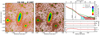 |
Fig. 2. Surface brightness image and profile of the galaxy CIG 340 (IC 2487). Left panel: r-band image. The scale of the colours represents the surface brightness of the image, and the scale is shown in the profile panel (right) following the y-axis scale. Middle panel: same image with the mask applied and the elliptical apertures of the dynamic position angle and ellipticity profile. Right panels: surface brightness profile (top), position angle (middle), and ellipticity (bottom) with respect to the radial distance in arcseconds (bottom) and kiloparsec (top). The red and green curves show the fit with dynamic and fixed elliptical apertures, respectively. The blue curve represents the fit with rectangular apertures. The position of the disc break (if any) is shown with the dashed elliptical aperture and the vertical dashed line in the middle and right panels, respectively. The dotted line in the right panel represents the radius at 25 mag arcsec−2. The figures for the whole sample of galaxies are given in Appendix B. |
3.3. Reliability of the profiles
In order to obtain reliable measurements in the extreme low surface brightness regime, numerous factors have to be taken into account. Most are related to the processing of the data and the instrumentation, such as data reduction and processing, scattered light as described by the point spread function (PSF), or the presence of reflections and artefacts in the images related to instrumentation. Additionally, the presence of Galactic cirrus in some images is ubiquitous and may produce confusion depending on the degree of contamination of the target.
As discussed in Sect. 2.2, the data processing was carried out using techniques designed to take the extremely low surface brightness features into account. This is noticeable in the absence of oversubtraction of the profiles (see Fig. 2) in the fainter regions, and it allowed us to achieve surface brightness profiles that are reliable below 30 mag arcsec2 in most cases. However, as noted by Sandin (2014), Karabal et al. (2017), Martínez-Lombilla & Knapen (2019), Gilhuly et al. (2022), the light scattered by the bright part of the galaxy itself through the PSF has a decisive impact on the photometric profiles in this extremely low surface brightness regime. In order to obtain better reliability, a proper PSF deconvolution of the galaxy has to be performed. However, because our data originate from several instruments over a very wide range in time (of the order of years), and because no specific observations of bright stars were carried out, we lack a PSF model for each epoch and telescope with which to perform the proper PSF deconvolution. Following Trujillo & Fliri (2016), we estimated that the photometric profiles were unaffected to a surface brightness of around 28 mag arcsec−2. Because disc breaks are found to take place at surfaces brightness levels no lower than 26 mag arcsec−2 (Gutiérrez et al. 2011; Pranger et al. 2017; Watkins et al. 2019), our reliability limit is more than sufficient to explore them. However, the lack of adequate PSF models rules out a potential quantitative study of truncations or stellar haloes in the outermost regions of the galaxies in our sample.
The presence of Galactic cirrus in our images is also problematic due to the extremely low brightness reached (cirrus indeed appears clearly in some of our images). The maximum possible surface brightness of these cirrus features is 26 mag arcsec2 (see Román et al. 2020). Considering that this problem affects mostly surface brightnesses below a value of approximately 26 mag arcsec−2, we can again conclude that this does not affect the study of disc breaks. It will, however, have a decisive impact on contaminating the outer regions of galaxies hiding possible interaction features. The presence of cirrus should therefore be taken into account in the study of potential minor interactions, as we describe below (Sect. 3.5).
3.4. Break identification and classification
We defined a disc break as an abrupt change in the slope of the exponential disc of a galaxy. Following Erwin et al. (2005) and Pohlen & Trujillo (2006), we defined three different types of profiles for our classification: Type I has a single exponential profile with no change in the slope; Type II has down-bending break, with a steeper outer region; and Type III has an up-bending break, with a steeper inner region. We only searched for the most prominent breaks that are the consequence of a change in the global structure and not due to a local change (e.g., an irregular morphology due to prominent H II regions). To characterise the breaks, we used two different approaches. First, given the small sample, we classified the break radii and type through a visual inspection of the surface brightness profiles. Second, we used the statistical approach of Watkins et al. (2019), where a change point analysis is applied to identify the break radius. This method searches for significant changes in the smooth derivative of the profile. We measured the slope of the surface brightness profile (as done in Pohlen & Trujillo 2006) using the four nearest points for each radial distance, and we smoothed the resulting slope with a median filter. We followed a classification similar to that of previous works (Pranger et al. 2017; Watkins et al. 2019) for the consistency of the comparison. Fig. 3 shows the break radii found by the two different methods. We estimated the errors as the resolution of the profiles in the region of the break (distance between each point). In most cases, both approaches converge to the same solution, although the automatic method finds the break 2.06 kpc closer to the galactic centre than visual inspection. We expect an offset, as explained in Watkins et al. (2019), due to the smoothing of the derivative of the profile and the cumulative sum, which can induce small offsets in the radius. We therefore decided to adopt the value of the radii found by the visual inspection. In Table 2 we indicate the classification of the different types of profiles in our sample, together with the values of the break radii, found visually, and the surface brightness levels at which the breaks occur.
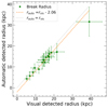 |
Fig. 3. Radii found via an automatic procedure as explained in Watkins et al. (2019) compared to those found via visual inspection of the profiles. The dotted grey line represents the 1:1 line, and the dashed orange line represents a linear fit to the data. The error bars were estimated using the distance to the next radial bins in the surface brightness profile at the distance at which the break was measured. |
Results of the break identification.
3.5. Identification of interactions
We visually inspected our sample in search of signatures of perturbations following the definitions of Martínez-Delgado et al. (2023), and references therein. The large field of view of our images corresponds to at least 100 kpc, which is enough to explore interactions with confidence. In order to provide a simple and general classification with which to introduce a perturbation parameter, we distinguished galaxies according to their morphology as follows. Tidal stream (T): The galaxy shows a tidal stream and is elongated. This is consistent with an in-falling satellite in current interaction. Halo-perturbed (H): The galaxy has asymmetries or debris in the outermost part of the disc. Cirrus (C): In the case of strong Galactic cirrus contamination, a correct interpretation of the degree of galaxy perturbation or interaction is not possible. In this case, we discarded the galaxy as intractable and excluded it from the statistics that imply using the presence of interactions. When a galaxy appears fairly symmetrical in morphology with no signs of disturbance, no classification is given. We describe interactions as effects from mergers in the outer regions of galaxies. These are distinguishable from lopsidedness potentially produced by gas (Bosma 2017) because our surface brightness limits allow us to explore the outer or halo regions of galaxies, beyond simply tracing the central morphology where star formation is dominant.
The result of this classification for each galaxy is shown in Table 2, and in Fig. 4 we show representative examples of the interaction classification scheme. In the top row panels, we show a symmetric non-classified (left), halo-perturbed (middle), and tidal stream (right) example. In the bottom panels, we show three different examples of galaxies with strong Galactic cirrus contamination that do not allow us to determine the presence or absence of potential interaction features in the galaxies.
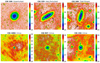 |
Fig. 4. Different examples of the interaction classification scheme. In the top panel, we show an unperturbed symmetric example (top left panel), CIG 100 (UGC 1863). The top middle and right panels show examples of perturbed galaxies. CIG 335 (NGC 2870) shows an overdensity in the halo region, and CIG 340 (IC 2487) shows a tidal stream in the southern region. All perturbation features are indicated with a black arrow. The bottom panels represent galaxies classified as cirrus-contaminated. CIG 1004 (NGC 7479), CIG 947 (NGC 7217), and CIG 154 (UGC 1706) are shown in the bottom left, middle, and right panels, respectively. These examples show considerable amounts of diffuse emission associated with Galactic cirrus only seen in our images. All of the images, except that of CIG 100, were smoothed with FABADA to enhance the structure. |
4. Results
We present below individual comments on each of the galaxies, with a short discussion of the decisions made in the different classifications. In Table 2 we show the results of the classification of profiles for each galaxy, together with the radius at which a break has been found (if any) and its surface brightness level.
– CIG 11 [UGC 139]: Although this galaxy could have been classified as Type III+II at 10 + 20 kpc (see the discussion by Watkins et al. 2019), we classify it as a Type II because additional flux originating from H II regions is seen in the inner disc region. This additional flux could be misinterpreted as Type III, although according to Pranger et al. (2017), Type III breaks occur farther away. Thus, for the sake of a fair comparison, we classify this as a Type II break at 19 kpc. We also consider this galaxy as unperturbed due to its symmetric structure. Diffuse cirrus emission is present, but this does not prevent the detection of interactions.
– CIG 33 [NGC 237]: We consider this a clear Type III with a break radius of ∼12 kpc and a perturbed halo. The diffuse emission around the galaxy is asymmetric, with a bump in the north-east region of the outskirts.
– CIG 59 [UGC 1167]: An exponential disc without a break, with a symmetric structure. Instrumental reflection of a nearby star is present, which, when correctly masked, does not contaminate the rest of the galaxy.
– CIG 94 [UGC 1706]: Galaxy with a down-bending Type II break at ∼10 kpc, without interaction signatures.
– CIG 96 [NGC 864]: This galaxy shows an up-bending Type III break at ∼16 kpc with a perturbed halo. Additional flux is visible in the north-east region of the disc outskirts.
– CIG 100 [UGC 1863]: Galaxy with a down-bending Type II break at 5 kpc, symmetric structure. Possible Type III break around 18.5 kpc at 28 mag arcsec−2. However, at this depth, we cannot distinguish between instrumental effects such as extended PSF contribution, as explained in Sect. 3.3.
– CIG 154 [UGC 3171]: Galaxy with an exponential disc with a symmetric structure. Indications of a larger spiral arm, at around ∼17 kpc, in the southern region. Filamentary cirrus prevents us from determining any faint interaction feature in the outer regions of the galaxy.
– CIG 279 [NGC 2644]: Galaxy with an exponential disc and symmetric structure. Diffuse cirrus emission would not prevent the detection of interaction features, if present. Possible Type III at ∼13 kpc, but the depth and presence of cirrus do not allow us to distinguish between the possible origins.
– CIG 329 [NGC 2862]: Galaxy with a Type II break at ∼16 kpc, clear tidal stream at the end of the disc in the south-east region. Instrumental reflection of a nearby star is present, which does not contaminate the rest of the galaxy when it is correctly masked.
– CIG 335 [NGC 2870]: This galaxy shows a Type II break at ∼15 kpc. There are signatures of overdensities and perturbations in the halo region, and therefore, we classify this as a perturbed halo. Figure 4 shows an enhanced image of the galaxy for greater clarity.
– CIG 340 [IC 2487]: Galaxy showing a Type II at ∼14 kpc, clear tidal stream in the southern region.
– CIG 512 [UGC 6903]: Symmetric galaxy with a Type II break at ∼9 kpc. Oversubstraction effects could cause the significant drop in brightness seen at 20 kpc, which can be a result of the Subaru pipeline.
– CIG 568 [UGC 8170]: Symmetric galaxy with a Type II break at ∼21 kpc.
– CIG 613 [UGC 9048]: The galaxy exhibits a Type II break at ∼40 kpc with signatures of a very faint and warped tidal stream. Appendix B shows an enhanced image with an arrow showing this stream.
– CIG 616 [UGC 9088]: Galaxy with an exponential disc, with an elliptical shape in the halo region with additional flux perpendicular to the major axis. The additional flux in clumps in the outermost regions indicate past interaction. Classified as perturbed halo.
– CIG 626 [NGC 5584]: Symmetric galaxy with a featureless disc profile, Type I.
– CIG 744 [UGC 10437]: Although this galaxy seems to have some fluctuations between 7 kpc and 15 kpc that could be classified as breaks, we classified as an exponential disc (Type I) it based on the constant global decrease in the average surface brightness in the disc. We identify the local fluctuations coming from clumpy H II regions of the arms. No features indicate interactions.
– CIG 772 [IC 1231]: Symmetric galaxy with a Type II break at 17 kpc.
– CIG 800 [NGC 6347]: Galaxy showing a Type II break at ∼19 kpc. The galaxy is fully embedded in a region that is heavily contaminated by cirrus, which prevents the classification of possible interaction features. Furthermore, several stars lie in the line of sight in the north-west region, and faint contamination due to the extended PSF can cause additional light at the end of the profile (see Sect. 3.3).
– CIG 838 [IC 1269]: Galaxy with an exponential Type I disc. From our optical imaging or the derived profile, we do not detect any signs of interaction, even though the northern spiral arm shows asymmetries with respect to the other spiral arm. Some diffuse cirrus emission is present, but not enough to prevent the detection of faint interaction features.
– CIG 947 [NGC 7217]: Although this object can be misinterpreted as an early-type galaxy, high-resolution colour images show spiral structures with two blue rings in the inner and outer regions. The radial profile exhibits a clear exponential disc. We see clear signatures of cirrus contamination (Fig. 4), which prevents any detection of possible interaction features.
– CIG 971 [UGC 12082]: Galaxy with an exponential disc, Type I. The galaxy is fully embedded in a region that is heavily contaminated by cirrus, which prevents the classification of possible interaction features. Furthermore, the field is crowded with stars. This contamination can be also be seen in the rectangular radial profile as a plateau at ∼28 mag arcsec−2 (as explained in Sect. 3.3).
– CIG 1002 [NGC 7451]: Galaxy showing a Type II break at 14 kpc. We detect a possible companion in the south-west region of the galaxy. However, no spectra are available to confirm the association of the two galaxies. We do not see any signature of interaction between them.
– CIG 1004 [NGC 7479]: Galaxy showing a Type II with a break radius of 15 kpc. The difference between the fixed and free ellipticity surface brightness profiles comes from the extended stellar bar. We are also able to see the same break with the rectangular aperture. The galaxy is fully embedded in a region that is heavily contaminated by cirrus (see Fig. 4), which prevents the classification of possible interaction features from deep optical imaging. The asymmetry of the galaxy disc and spiral arms is well known, however, and may indicate a minor merger origin (e.g., Laine & Gottesman 1998).
– CIG 1047 [UGC 12857]: Galaxy showing a Type II break at 8 kpc. We see a warp in the southern part of the outer disc, and therefore, we classify this galaxy as a perturbed halo. Diffuse cirrus emission is present that would not prevent the detection of interaction features, if present.
In total, among 25 galaxies, we identify 9 Type I single exponential galaxies with no significant break, 14 Type II down-bending break galaxies, and 2 Type III up-bending break galaxies. The overall statistics of the sample are 36%±10% Type I, 56%±10% Type II, and 8%±5% Type III break galaxies. We estimate the uncertainties assuming a binomial distribution,  [%], where f is the fraction of galaxies within each type, and N is the total number of galaxies in our sample (N = 25).
4.1. Break type versus interactions
We find five galaxies with strong contamination by Galactic cirrus clouds that do not allow us to confirm or rule out interactions. These five galaxies were therefore excluded from this analysis. Among the remaining 20, we find eight galaxies with interaction signatures. Of these, four show asymmetries in the halo, three have tidal streams, and the remaining one shows both tidal streams and halo asymmetries. Therefore, 40% ± 14% of the isolated galaxies in our classified sample show interactions; out of these galaxies, 25%±10% show an asymmetric halo, and 20% ± 8% show some tidal streams. We found 12 galaxies (60% ± 17%) with no interaction features.
Because of the small sample size, we considered any type of interaction as a single class named perturbed galaxies (8 galaxies) (with interactions), while the remaining galaxies (that lack cirrus contamination) were classified as unperturbed (12 galaxies). In the right panel of Fig. 5, we show the fraction of perturbed and unperturbed galaxies for each type of break. We found that for Type I breaks, 6 (83%±37%) are unperturbed galaxies and one (17%±17%) is perturbed; for Type II, 8 (58%±22%) are unperturbed and 5 (42%±19%) are perturbed. Finally, we find that the 2 galaxies with Type III are perturbed (100%±71%). We estimated the errors assuming Poisson statistics because we have only a few of galaxy in each type.
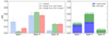 |
Fig. 5. Frequency of the disc break type and the interaction signatures of our sample of galaxies. Left: normalised distribution of the frequency of the types of breaks found in this work (left, blue) and in Pranger et al. (2017) for their field (middle, green) and cluster (right, red) samples. Right: normalised distribution of the frequency of the types of breaks. Galaxies that are strongly contaminated by cirrus are excluded from this figure. We also show the contribution of unperturbed (blue) and perturbed (green) galaxies for each type of break. |
The low number of galaxies in our sample is insufficient to allow us to make strong statements. However, we find certain indications that are undoubtedly interesting. First, both Type III galaxies (CIG 33 and CIG 96) appear strongly perturbed. This is noticeable in the images in the appendix, which show that these two galaxies have an expanded halo with clear signs of strong disturbance, possibly due to a recent major merger. Second, we find a significantly higher fraction of perturbed galaxies (42% ± 19%) among Type II break hosts than among Type I break hosts (17% ± 17%).
4.2. Break type versus environment
In the left panel of Fig. 5, we show the fraction of surface brightness profile types in our sample of isolated galaxies in comparison with the previous work by Pranger et al. (2017), who explored the surface brightness type in a sample of 700 disc galaxies at low redshift (z < 0.063) using SDSS data. These galaxies were classified according to their environment into field (low density) and cluster galaxies (high density). The fractions of Type I, II, and III discs found by Pranger et al. (2017) are 29 (6%±1%), 343 (66%±2%), and 149 (29%±2%) in the field sample and 27 (15%±3%), 98 (56%±4%), and 50 (29%±3%) in the cluster sample. For the sake of a fair comparison, we estimated the Pranger et al. (2017) uncertainties in the same way as we did for our results. We compare these statistics with the sample of isolated galaxies from our work. As illustrated in the left panel of Fig. 5, we find a considerably higher fraction of isolated Type I galaxies and a lower fraction of isolated Type III galaxies than what was found by Pranger et al. (2017) for field galaxies and clusters. The results for Type II are similar for the different environments.
A Kolmogorov–Smirnov statistical test proves that our results are significantly different from those of Pranger et al. (2017) (P-value < 0.01). The highest difference between our results and those of the Pranger et al. (2017) sample is found for Type I discs. We find six times more single exponential discs in our isolated sample. This difference holds when compared to other studies, such as that by Gutiérrez et al. (2011), who found around ∼10 − 15% of Type I disc in field late-type spirals, around two to three times less often than we did. We also find a much lower fraction, around seven times lower, of Type III discs than Pranger et al. (2017).
In Fig. 6 we show a correlation test between the degree of isolation and the disc type of the galaxies in our sample. We plot the local number density of neighbours galaxies ηk, p and the tidal strength QKar, p obtained by Argudo-Fernández et al. (2013) for the 18 galaxies in our sample for which these parameters were calculated. An increasing value for ηk, p or QKar, p indicates a higher environmental density. We show as a comparison these parameters for other galaxy catalogues, including galaxies located in regions of higher density. In particular, we show values for isolated pairs of galaxies (KGP; Karachentsev 1972), galaxy triplets (KTG; Karachentseva et al. 1979), galaxies in compact groups (HCG; Hickson 1982), and galaxies in Abell clusters (ACO; Abell 1958; Abell et al. 1989) computed by Argudo-Fernández et al. (2013). We find that the galaxies in our sample tend to be located at low values of ηk, p and QKar, p, confirming their location in regions of low environmental density, which is a consequence of the sample selection criteria. The colour code indicates the type of surface brightness profile, and the symbols show the two populations according to our classification into perturbed and unperturbed galaxies. The average values of the ηk, p and QKar, p parameters for each break type are indicated by colour bars, and for the unperturbed and perturbed population, they are shown with symbols. For the galaxies in our sample, the different disc types tend to be located on average in regions of similar density. These regions all have a very low density.
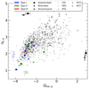 |
Fig. 6. Photometric isolation parameter for 18 galaxies of our sample, and the local number density of neighbour galaxies, ηk, p, compared to the tidal strength, QKar, p, from Argudo-Fernández et al. (2013). The colour code represents the type of disc: blue, green, and red for Types I, II, and III, respectively. The mean values of each type are represented by the line close to the axis (bottom and left) with its corresponding error. Circles and stars represent unperturbed and perturbed galaxies, respectively. The mean values of perturbed and unperturbed galaxies are represented by the symbols close to the axis (upper and right) with their corresponding error. The crosses correspond to galaxies that were not classified due to galactic cirrus. Background grey values represent galaxies from different samples (see Sect. 4 for details). |
5. Discussion
We presented deep optical imaging of a sample of 25 isolated galaxies from the AMIGA project in order to reach low surface brightness limits. The nominal surface brightness limits achieved are μr,lim > 29.5 mag arcsec−2 [3σ; 10″ × 10″] and μL,lim > 28.5 mag arcsec−2 [3σ; 10″ × 10″] for the three galaxies observed with the JRT. Because of our careful data processing, our images show an absence of oversubtracted regions and a high efficiency in the detection of extreme low surface brightness features.
The depth of our data is more than 1 mag arcsec−2 (r band) deeper than that in preceding studies (see e.g., Martínez-Delgado et al. 2023, using the Legacy Survey). This gives us the possibility to search for minor interaction signatures at very low surface brightness. A representative example of this quantitative leap is shown in Fig. 1, where we compare images of CIG 340 (IC 2487) with SDSS and Legacy Survey data. This comparison clearly shows that only our data enable detecting the clear interaction that CIG 340 is undergoing with a low-mass satellite. This appears as a tidal stream with a surface brightness of about 26.8 − 27.3 mag arcsec−2 and an extension of about ∼116 arcsec (35 kpc). This is not detectable in shallower optical data.
The potential detection of minor interactions has a decisive impact on the interpretation of galaxy properties, and the isolated galaxy CIG 340 is a perfect example. Shallow optical images of CIG 340 revealed a fairly symmetric disc, albeit with a small disc warp. Additionally, the H I-integrated spectra from single-dish observations showed a very symmetric profile (see Espada et al. 2011). More recent high-resolution interferometric observations by Scott et al. (2014) revealed a striking asymmetry of the H I component of CIG 340, with 6% of the H I mass located in an extension of the disc to the north. These findings led Scott et al. (2014) to propose two different hypotheses to explain them. On the one hand, this H I asymmetry could be caused by a minor interaction with a satellite that was not detected in the optical images available at the time. On the other hand, it could be due to some internal secular process, for example the result of a long-lived dark matter halo asymmetry. More recent work by Kipper et al. (2020) proposed that the gravitational interaction of a background medium of dark matter particles in the surroundings of CIG 340 is capable of inducing a dynamical friction enough to cause the H I asymmetries observed by Scott et al. (2014). In light of the results of our work, we can affirm that the H I asymmetries observed in the isolated galaxy CIG 340 are most likely caused by a minor interaction, the signatures of which we have unveiled for the first time.
The galaxy CIG 96 (NGC 864) is another well-studied isolated galaxy. Recent work detected two H I asymmetries in the north-west and south-east regions of the galaxy (Ramírez-Moreta et al. 2018) that were not detected in the optical range. The main hypotheses to explain the HI features of CIG 96 are possible accreted companions and cold gas accretion. However, Ramírez-Moreta et al. (2018) ruled out the possibility of major merger events due to the isolation criteria (discarded possible interactions in the last 2.7 Gyr). Despite the high degree of isolation of this galaxy, with our deep data, we are able to detect a larger external faint halo in the galaxy, which along with its Type III profile suggests that this galaxy might have experimented a recent merger event causing the extended emission of light (e.g., Laurikainen & Salo 2001; Lotz et al. 2008; Borlaff et al. 2014; Barrera-Ballesteros et al. 2015; Pfeffer et al. 2022).
The possibility of achieving surface brightness levels as low as those shown here offers a new decisive parameter to explain some morphological features in galaxies. This would not only be useful to investigate the main reasons for H I asymmetries of galaxies, but also in other fields, such as the possible induction of active galactic nuclei (AGN) by minor interactions in galaxies, among many others. These issues will be investigated in future works.
The types of discs in the isolated galaxies from our sample show significant differences with respect to the results of previously studied samples in other environments. We find a significantly higher fraction of Type I and a significantly lower fraction of Type III profiles than in works by Pranger et al. (2017) and Gutiérrez et al. (2011) for denser environments. This is a striking result that we discuss further now.
Type III profiles can be produced by mergers of galaxies (e.g., Laurikainen & Salo 2001; Borlaff et al. 2014; Pfeffer et al. 2022, and references therein). The low number of Type III profiles in our sample of isolated galaxies agrees with this statement because undoubtedly, a lower density would imply a lower merger ratio. Additionally and importantly, the only two Type III galaxies found in our sample (CIG 33 and CIG 96) show a disturbed morphology with a puffed-up external halo, which is compatible with a recent major merger (Lotz et al. 2008; Barrera-Ballesteros et al. 2015).
Type II galaxies are widely agreed to be the result of discs with breaks caused by a star formation threshold (e.g., Tang et al. 2020; Pfeffer et al. 2022). A cessation or decrease in star formation would tend to homogenise through stellar migration effects (Sánchez-Blázquez et al. 2009) the stellar populations and produce a Type I profile (e.g., Pfeffer et al. 2022). In our case, this can hardly be tested directly because no star formation measurements are available for our sample. However, an indirect indication that this is the case is the considerably higher fraction of perturbed Type II (42% ± 19%) galaxies when compared to Type I (17% ± 17%) galaxies. While the rate of star formation may depend on various circumstances such as the rate of pristine gas inflow, it is known that satellite interactions are capable of triggering star formation (Barton et al. 2000; Alonso et al. 2004; Knapen et al. 2015; Mesa et al. 2021), which would be in accordance with our findings. The low ratio of perturbations detected in Type I discs galaxies in our results and the lower specific star formation rate in isolated galaxies than in higher-density environments (Lisenfeld et al. 2011; Melnyk et al. 2015; Domínguez-Gómez et al. 2023) suggests that unperturbed galaxies, evolving slowly with a low star formation rate, could explain the high rate of Type I discs in isolated galaxies.
6. Conclusions
We studied a sample of 25 isolated galaxies from the AMIGA revised CIG catalogue that lack main companions to identify how internal or external processes impact the galaxy discs. We conducted a diverse observational campaign using the INT, VST, JRT, and archival data from HSC-SSP to obtain unprecedentedly deep images. We measured the surface brightness profiles and classified the galaxies according to their disc break (Type I is a single exponential, Type II is a down-bending, and Type III is an up-bending galaxy) and according to interaction signatures (tidal stream, halo perturbation, and unperturbed). The conclusions of our work are listed below.
-
Our images have a similar depth as those to come from future surveys, such as the LSST, through careful data processing and background subtraction. The nominal surface brightness limit of the images is μr,lim > 29.5 mag arcsec−2 [3σ; 10″ × 10″]. The data processing is optimized to preserve low surface brightness features.
-
Thanks to the image depth obtained, we can trace interaction signatures in galaxies classified as isolated (see Fig. 1). However, five galaxies are affected by cirrus, and we could not explore any interaction signatures. They were excluded from this analysis. We find that 25% ± 10% of the galaxies in our sample show an asymmetric halo and 20% ± 10% show a tidal stream (see Fig. 4). In total, 40% ± 14% show signs of interactions.
-
We are able to produce reliable surface brightness profiles down to a critical surface brightness of ≳30 mag arcsec−2 for all of the galaxies in our sample (see Appendix B).
-
We successfully classified the disc type in all the galaxies in our sample. We identify 9 (36%±5%) Type I discs with no significant break, 14 (56%±7%) Type II down-bending discs, and 2 (8%±3%) Type III up-bending discs.
-
The fraction of perturbed galaxies correlates with the type of disc. We identify 17%±17%, 42%±19%, and 100%±71% perturbed galaxies with Type I, II, and III discs, respectively.
-
We find significantly higher Type I and lower Type III frequencies with respect to other studies (e.g., Pranger et al. 2017; Gutiérrez et al. 2011) with more perturbed galaxies in Type II and III than in Type I. This agrees with the proposed formation scenario in which Type III discs are formed via interactions such as major mergers (see Laine et al. 2014; Watkins et al. 2019), and Type II discs stem from a star formation threshold. The increased fraction of Type I discs with respect to that in other samples could be attributed to the low ratio of disturbance in our sample of isolated galaxies.
In the near future, the advent of the next-generation optical and infrared surveys (e.g., LSST or Euclid) will increase the number of galaxies that are observed at surface brightness limits equivalent to those that we present in this work by several orders of magnitude. This will allow us to further strengthen and refine our statements if the data reduction and analysis allows for the detection of low surface brightness.
Acknowledgments
We thank Ignacio Trujillo for helpful insights about this work and Aaron Watkins for providing us with the implementation of the automatic break detection method. PMSA, JHK, and JR acknowledge financial support from the State Research Agency (AEI-MCINN) of the Spanish Ministry of Science and Innovation under the grant “The structure and evolution of galaxies and their central regions” with reference PID2019-105602GBI00/10.13039/501100011033, from the ACIISI, Consejería de Economía, Conocimiento y Empleo del Gobierno de Canarias and the European Regional Development Fund (ERDF) under grant with reference PROID2021010044, and from IAC project P/300724, financed by the Ministry of Science and Innovation, through the State Budget and by the Canary Islands Department of Economy, Knowledge and Employment, through the Regional Budget of the Autonomous Community. JR acknowledges funding from University of La Laguna through the Margarita Salas Program from the Spanish Ministry of Universities ref. UNI/551/2021-May 26, and under the EU Next Generation. LVM acknowledges financial support from grants CEX2021-001131-S funded by MCIN/AEI/ 10.13039/501100011033, RTI2018-096228-B-C31 and PID2021-123930OB-C21 by MCIN/AEI/ 10.13039/501100011033, by “ERDF A way of making Europe” and by the “European Union” and from IAA4SKA (R18-RT-3082) funded by the Economic Transformation, Industry, Knowledge and Universities Council of the Regional Government of Andalusia and the European Regional Development Fund from the European Union. SC acknowledges funding from the State Research Agency (AEI-MCINN) of the Spanish Ministry of Science and Innovation under the grant “Thick discs, relics of the infancy of galaxies” with reference PID2020-113213GA-I00. MAF acknowledges support from FONDECYT iniciación project 11200107 and the Emergia program (EMERGIA20_38888) from Consejería de Transformación Económica, Industria, Conocimiento y Universidades and University of Granada. PMSA and LVM acknowledge the Spanish Prototype of an SRC (SPSRC) service and support funded by the Spanish Ministry of Science, Innovation and Universities, by the Regional Government of Andalusia, by the European Regional Development Funds and by the European Union NextGenerationEU/PRTR. The SPSRC acknowledges financial support from the State Agency for Research of the Spanish MCIU through the “Center of Excellence Severo Ochoa” award to the Instituto de Astrofísica de Andalucía (SEV-2017-0709) and from the grant CEX2021-001131-S funded by MCIN/AEI/ 10.13039/501100011033. Based on observations made with the Isaac Newton Telescope operated on the island of La Palma by the Isaac Newton Group of Telescopes in the Spanish Observatorio del Roque de los Muchachos of the Instituto de Astrofísica de Canarias. The WFC imaging was obtained as part of the programs C163/13A, C106/13B, and C106/14A. Based on observations collected at the European Organisation for Astronomical Research in the Southern Hemisphere under ESO programme(s) 098.B-0775(A), 093.B-0894(A). Based on data collected at the Subaru Telescope and retrieved from the HSC data archive system, which is operated by Subaru Telescope and Astronomy Data Center at National Astronomical Observatory of Japan.
References
- Abazajian, K. N., Adelman-McCarthy, J. K., Agüeros, M. A., et al. 2009, ApJS, 182, 543 [Google Scholar]
- Abell, G. O. 1958, ApJS, 3, 211 [NASA ADS] [CrossRef] [Google Scholar]
- Abell, G. O., Corwin, H. G., & Olowin, R. P. 1989, ApJS, 70, 1 [Google Scholar]
- Abraham, R. G., & van Dokkum, P. G. 2014, PASP, 126, 55 [Google Scholar]
- Aihara, H., Arimoto, N., Armstrong, R., et al. 2018, PASJ, 70, S4 [NASA ADS] [Google Scholar]
- Aihara, H., AlSayyad, Y., Ando, M., et al. 2019, PASJ, 71, 114 [Google Scholar]
- Akhlaghi, M. 2019, ArXiv e-prints [arXiv:1909.11230] [Google Scholar]
- Akhlaghi, M., & Ichikawa, T. 2015, ApJS, 220, 1 [Google Scholar]
- Alonso, M. S., Tissera, P. B., Coldwell, G., et al. 2004, MNRAS, 352, 1081 [NASA ADS] [CrossRef] [Google Scholar]
- Arakelian, M. A., & Magtesian, A. P. 1981, Astrofizika, 17, 53 [NASA ADS] [Google Scholar]
- Argudo-Fernández, M., Verley, S., Bergond, G., et al. 2013, A&A, 560, A9 [NASA ADS] [CrossRef] [EDP Sciences] [Google Scholar]
- Astropy Collaboration (Robitaille, T. P., et al.) 2013, A&A, 558, A33 [NASA ADS] [CrossRef] [EDP Sciences] [Google Scholar]
- Astropy Collaboration (Price-Whelan, A. M., et al.) 2018, AJ, 156, 123 [Google Scholar]
- Azzollini, R., Trujillo, I., & Beckman, J. E. 2008, ApJ, 679, L69 [NASA ADS] [CrossRef] [Google Scholar]
- Bakos, J., & Trujillo, I. 2012, ArXiv e-prints [arXiv:1204.3082] [Google Scholar]
- Bakos, J., Trujillo, I., & Pohlen, M. 2008, ApJ, 683, L103 [NASA ADS] [CrossRef] [Google Scholar]
- Baldry, I. K., Balogh, M. L., Bower, R. G., et al. 2006, MNRAS, 373, 469 [Google Scholar]
- Balogh, M. L., Baldry, I. K., Nichol, R., et al. 2004, ApJ, 615, L101 [Google Scholar]
- Barton, E. J., Geller, M. J., & Kenyon, S. J. 2000, ApJ, 530, 660 [NASA ADS] [CrossRef] [Google Scholar]
- Barrera-Ballesteros, J. K., García-Lorenzo, B., Falcón-Barroso, J., et al. 2015, A&A, 582, A21 [NASA ADS] [CrossRef] [EDP Sciences] [Google Scholar]
- Bertin, E., & Arnouts, S. 1996, A&AS, 117, 393 [NASA ADS] [CrossRef] [EDP Sciences] [Google Scholar]
- Bertin, E. 2006, Astronomical Data Analysis Software and Systems XV, 351, 112 [NASA ADS] [Google Scholar]
- Borlaff, A., Eliche-Moral, M. C., Rodríguez-Pérez, C., et al. 2014, A&A, 570, A103 [NASA ADS] [CrossRef] [EDP Sciences] [Google Scholar]
- Borlaff, A., Eliche-Moral, M. C., Beckman, J. E., et al. 2018, A&A, 615, A26 [NASA ADS] [EDP Sciences] [Google Scholar]
- Borlaff, A., Trujillo, I., Román, J., et al. 2019, A&A, 621, A133 [NASA ADS] [CrossRef] [EDP Sciences] [Google Scholar]
- Bosma, A. 2017, Outskirts of Galaxies, 434, 209 [NASA ADS] [CrossRef] [Google Scholar]
- Dark Energy Survey Collaboration (Abbott, T., et al.) 2016, MNRAS, 460, 1270 [Google Scholar]
- Debattista, V. P., Mayer, L., Carollo, C. M., et al. 2006, ApJ, 645, 209 [Google Scholar]
- Domínguez-Gómez, J., Pérez, I., Ruiz-Lara, T., et al. 2023, Nature, 619, 269 [CrossRef] [Google Scholar]
- Duc, P.-A., Cuillandre, J.-C., Karabal, E., et al. 2015, MNRAS, 446, 120 [Google Scholar]
- de Vaucouleurs, G. 1958, ApJ, 128, 465 [NASA ADS] [CrossRef] [Google Scholar]
- Eliche-Moral, M. C., Borlaff, A., Beckman, J. E., et al. 2015, A&A, 580, A33 [NASA ADS] [CrossRef] [EDP Sciences] [Google Scholar]
- Erwin, P., Beckman, J. E., & Pohlen, M. 2005, ApJ, 626, L81 [Google Scholar]
- Erwin, P., Gutiérrez, L., & Beckman, J. E. 2012, ApJ, 744, L11 [NASA ADS] [CrossRef] [Google Scholar]
- Espada, D., Verdes-Montenegro, L., Huchtmeier, W. K., et al. 2011, A&A, 532, A117 [NASA ADS] [CrossRef] [EDP Sciences] [Google Scholar]
- Fliri, J., & Trujillo, I. 2016, MNRAS, 456, 1359 [Google Scholar]
- Freeman, K. C. 1970, ApJ, 160, 811 [Google Scholar]
- Gilhuly, C., Merritt, A., Abraham, R., et al. 2022, ApJ, 932, 44 [NASA ADS] [CrossRef] [Google Scholar]
- Gutiérrez, L., Erwin, P., Aladro, R., et al. 2011, AJ, 142, 145 [CrossRef] [Google Scholar]
- Haigh, C., Chamba, N., Venhola, A., et al. 2021, A&A, 645, A107 [NASA ADS] [CrossRef] [EDP Sciences] [Google Scholar]
- Herpich, J., Stinson, G. S., Rix, H.-W., et al. 2017, MNRAS, 470, 4941 [NASA ADS] [CrossRef] [Google Scholar]
- Hickson, P. 1982, ApJ, 255, 382 [NASA ADS] [CrossRef] [Google Scholar]
- Huang, Q., & Fan, L. 2022, ApJS, 262, 39 [NASA ADS] [CrossRef] [Google Scholar]
- Huchra, J., & Thuan, T. X. 1977, ApJ, 216, 694 [NASA ADS] [CrossRef] [Google Scholar]
- Infante-Sainz, R., Trujillo, I., & Román, J. 2020, MNRAS, 491, 5317 [Google Scholar]
- Jablonka, P., Tafelmeyer, M., Courbin, F., et al. 2010, A&A, 513, A78 [NASA ADS] [CrossRef] [EDP Sciences] [Google Scholar]
- Jedrzejewski, R. I. 1987, MNRAS, 226, 747 [Google Scholar]
- Jiang, L., Fan, X., Bian, F., et al. 2014, ApJS, 213, 12 [NASA ADS] [CrossRef] [Google Scholar]
- Johnston, K. V., Sackett, P. D., & Bullock, J. S. 2001, ApJ, 557, 137 [NASA ADS] [CrossRef] [Google Scholar]
- Johnston, K. V., Bullock, J. S., Sharma, S., et al. 2008, ApJ, 689, 936 [Google Scholar]
- Jones, M. G., Espada, D., Verdes-Montenegro, L., et al. 2018, A&A, 609, A17 [NASA ADS] [CrossRef] [EDP Sciences] [Google Scholar]
- Karabal, E., Duc, P.-A., Kuntschner, H., et al. 2017, A&A, 601, A86 [NASA ADS] [CrossRef] [EDP Sciences] [Google Scholar]
- Karachentsev, I. D. 1972, Soobshcheniya Spetsial’noj Astrofizicheskoj Observatorii, 7, 1 [Google Scholar]
- Karachentseva, V. E. 1973, Soobshcheniya Spetsial’noj Astrofizicheskoj Observatorii, 8, 3 [Google Scholar]
- Karachentseva, V. E., Karachentsev, I. D., & Shcherbanovsky, A. L. 1979, Astrofizicheskie Issledovaniia Izvestiya Spetsial’noj Astrofizicheskoj Observatorii, 11, 3 [Google Scholar]
- Kipper, R., Benito, M., Tenjes, P., et al. 2020, MNRAS, 498, 1080 [NASA ADS] [CrossRef] [Google Scholar]
- Knapen, J. H., Shlosman, I., & Peletier, R. F. 2000, ApJ, 529, 93 [NASA ADS] [CrossRef] [Google Scholar]
- Knapen, J. H., Cisternas, M., & Querejeta, M. 2015, MNRAS, 454, 1742 [NASA ADS] [CrossRef] [Google Scholar]
- Kormendy, J., & Kennicutt, R. C. 2004, ARA&A, 42, 603 [Google Scholar]
- Laine, S., & Gottesman, S. T. 1998, MNRAS, 297, 1041 [CrossRef] [Google Scholar]
- Laine, S., Knapen, J. H., Muñoz-Mateos, J.-C., et al. 2014, MNRAS, 444, 3015 [NASA ADS] [CrossRef] [Google Scholar]
- Lang, D., Hogg, D. W., Mierle, K., et al. 2010, AJ, 139, 1782 [NASA ADS] [CrossRef] [Google Scholar]
- Laurikainen, E., & Salo, H. 2001, MNRAS, 324, 685 [NASA ADS] [CrossRef] [Google Scholar]
- Lisenfeld, U., Espada, D., Verdes-Montenegro, L., et al. 2011, A&A, 534, A102 [NASA ADS] [CrossRef] [EDP Sciences] [Google Scholar]
- Lotz, J. M., Jonsson, P., Cox, T. J., et al. 2008, MNRAS, 391, 1137 [CrossRef] [Google Scholar]
- Maltby, D. T., Gray, M. E., Aragón-Salamanca, A., et al. 2012, MNRAS, 419, 669 [NASA ADS] [CrossRef] [Google Scholar]
- Martin, G., Bazkiaei, A. E., Spavone, M., et al. 2022, MNRAS, 513, 1459 [NASA ADS] [CrossRef] [Google Scholar]
- Martínez-Delgado, D. 2019, Highlights on Spanish Astrophysics X, 146 [Google Scholar]
- Martínez-Delgado, D., D’Onghia, E., Chonis, T. S., et al. 2015, AJ, 150, 116 [CrossRef] [Google Scholar]
- Martínez-Delgado, D., Cooper, A. P., Román, J., et al. 2023, A&A, 671, A141 [NASA ADS] [CrossRef] [EDP Sciences] [Google Scholar]
- Martínez-Lombilla, C., & Knapen, J. H. 2019, A&A, 629, A12 [NASA ADS] [CrossRef] [EDP Sciences] [Google Scholar]
- Martín-Navarro, I., Bakos, J., Trujillo, I., et al. 2012, MNRAS, 427, 1102 [Google Scholar]
- Martínez-Serrano, F. J., Serna, A., Doménech-Moral, M., & Domínguez-Tenreiro, R. 2009, ApJ, 705, L133 [CrossRef] [Google Scholar]
- Melnyk, O., Karachentseva, V., & Karachentsev, I. 2015, MNRAS, 451, 1482 [NASA ADS] [CrossRef] [Google Scholar]
- Mesa, V., Alonso, S., Coldwell, G., et al. 2021, MNRAS, 501, 1046 [Google Scholar]
- Mihos, J. C. 2019, ArXiv e-prints [arXiv:1909.09456] [Google Scholar]
- Mihos, J. C., Durrell, P. R., Ferrarese, L., et al. 2015, ApJ, 809, L21 [Google Scholar]
- Mihos, J. C., Harding, P., Feldmeier, J. J., et al. 2017, ApJ, 834, 16 [Google Scholar]
- Muñoz-Mateos, J. C., Sheth, K., Regan, M., et al. 2015, ApJS, 219, 3 [Google Scholar]
- Patterson, F. S.1940, BHar, 914, 9 [NASA ADS] [Google Scholar]
- Pfeffer, J. L., Bekki, K., Forbes, D. A., et al. 2022, MNRAS, 509, 261 [Google Scholar]
- Pranger, F., Trujillo, I., Kelvin, L. S., et al. 2017, MNRAS, 467, 2127 [NASA ADS] [CrossRef] [Google Scholar]
- Pohlen, M., & Trujillo, I. 2006, A&A, 454, 759 [NASA ADS] [CrossRef] [EDP Sciences] [Google Scholar]
- Pohlen, M., Dettmar, R.-J., Lütticke, R., & Aronica, G. 2002, A&A, 392, 807 [NASA ADS] [CrossRef] [EDP Sciences] [Google Scholar]
- Ramírez-Moreta, P., Verdes-Montenegro, L., Blasco-Herrera, J., et al. 2018, A&A, 619, A163 [NASA ADS] [CrossRef] [EDP Sciences] [Google Scholar]
- Román, J., & Trujillo, I. 2018, Res. Notes Am. Astron. Soc., 2, 144 [Google Scholar]
- Román, J., Trujillo, I., & Montes, M. 2020, A&A, 644, A42 [NASA ADS] [CrossRef] [EDP Sciences] [Google Scholar]
- Román, J., Castilla, A., & Pascual-Granado, J. 2021, A&A, 656, A44 [NASA ADS] [CrossRef] [EDP Sciences] [Google Scholar]
- Román, J., Rich, R. M., Ahvazi, N., et al. 2023, A&A, submitted, [arXiv:2305.03073] [Google Scholar]
- Roškar, R., Debattista, V. P., Stinson, G. S., et al. 2008, ApJ, 675, L65 [Google Scholar]
- Ruiz-Lara, T., Pérez, I., Florido, E., et al. 2016, MNRAS, 456, L35 [NASA ADS] [CrossRef] [Google Scholar]
- Sánchez-Alarcón, P. M., & Ascasibar, Y. 2023, RAS Techn. Instrum., 2, 129 [CrossRef] [Google Scholar]
- Sánchez-Blázquez, P., Courty, S., Gibson, B. K., & Brook, C. B. 2009, MNRAS, 398, 591 [CrossRef] [Google Scholar]
- Sandin, C. 2014, A&A, 567, A97 [NASA ADS] [CrossRef] [EDP Sciences] [Google Scholar]
- Schlafly, E. F., & Finkbeiner, D. P. 2011, ApJ, 737, 103 [Google Scholar]
- Schwarzkopf, U., & Dettmar, R.-J. 2001, A&A, 373, 402 [NASA ADS] [CrossRef] [EDP Sciences] [Google Scholar]
- Scott, T. C., Sengupta, C., Verdes Montenegro, L., et al. 2014, A&A, 567, A56 [NASA ADS] [CrossRef] [EDP Sciences] [Google Scholar]
- Slater, C. T., Harding, P., & Mihos, J. C. 2009, PASP, 121, 1267 [Google Scholar]
- Staudaher, S. M., Dale, D. A., & van Zee, L. 2019, MNRAS, 486, 1995 [NASA ADS] [CrossRef] [Google Scholar]
- Sulentic, J. W., Verdes-Montenegro, L., Bergond, G., et al. 2006, A&A, 449, 937 [NASA ADS] [CrossRef] [EDP Sciences] [Google Scholar]
- Tang, Y., Chen, Q., Zhang, H.-X., et al. 2020, ApJ, 897, 79 [NASA ADS] [CrossRef] [Google Scholar]
- Thomas, D., Maraston, C., Bender, R., et al. 2005, ApJ, 621, 673 [NASA ADS] [CrossRef] [Google Scholar]
- Trujillo, I., & Fliri, J. 2016, ApJ, 823, 123 [Google Scholar]
- Trujillo, I., D’Onofrio, M., Zaritsky, D., et al. 2021, A&A, 654, A40 [NASA ADS] [CrossRef] [EDP Sciences] [Google Scholar]
- van der Kruit, P. C. 1979, A&AS, 38, 15 [NASA ADS] [Google Scholar]
- van der Kruit, P. C., & Searle, L. 1981a, A&A, 95, 105 [NASA ADS] [Google Scholar]
- van der Kruit, P. C., & Searle, L. 1981b, A&A, 95, 116 [NASA ADS] [Google Scholar]
- Varela, J., Moles, M., Márquez, I., et al. 2004, A&A, 420, 873 [NASA ADS] [CrossRef] [EDP Sciences] [Google Scholar]
- Verdes-Montenegro, L., Sulentic, J., Lisenfeld, U., et al. 2005, A&A, 436, 443 [NASA ADS] [CrossRef] [EDP Sciences] [Google Scholar]
- Verley, S., Odewahn, S. C., Verdes-Montenegro, L., et al. 2007a, A&A, 470, 505 [NASA ADS] [CrossRef] [EDP Sciences] [Google Scholar]
- Verley, S., Leon, S., Verdes-Montenegro, L., et al. 2007b, A&A, 472, 121 [NASA ADS] [CrossRef] [EDP Sciences] [Google Scholar]
- Wang, J., Zheng, Z., D’Souza, R., et al. 2018, MNRAS, 479, 4292 [NASA ADS] [CrossRef] [Google Scholar]
- Watkins, A. E., Mihos, J. C., & Harding, P. 2016, ApJ, 826, 59 [Google Scholar]
- Watkins, A. E., Laine, J., Comerón, S., et al. 2019, A&A, 625, A36 [NASA ADS] [CrossRef] [EDP Sciences] [Google Scholar]
- Zernike, von F. 1934, Physica, 1, 689 [NASA ADS] [CrossRef] [Google Scholar]
- Zheng, Z., Thilker, D. A., & Heckman, T. M. 2015, ApJ, 800, 120 [NASA ADS] [CrossRef] [Google Scholar]
Appendix A: SExtractor configuration parameters.
The parameters that were not set to their default values are
CHECKIMAGE_TYPE SEGMENTATION
DEBLEND_MINCONT 0.005
DEBLEND_NTHRESH 32
BACK_SIZE 20
DETECT_THRESH 0.9
Appendix B: Images, masks, and surface brightness radial profiles.
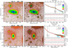 |
Fig. B.1. Surface brightness images and profiles for all the galaxies in our sample. Left panel: r-band or luminance images for the galaxy. The ID of each galaxy is shown above. The scale of the colours represents the surface brightness of the image, and the scale is shown in the profile panel (right) following the y-axis scale. Middle panel: Same image with the mask applied and the elliptical apertures of the dynamic positional angle and ellipticity profile. Right panel: Surface brightness profile (top), positional angle (middle), and ellipticity (bottom) as a function of the radius in arcseconds (bottom) and kiloparsec (top). The red and green line show the dynamic and fixed elliptical apertures, respectively. The blue line represents the profiles obtained from rectangular apertures. The position of the disc break (if any) is shown with the vertical and elliptical aperture of the dashed line. The dotted line in the right panel represents the radius at 25 mag arcsec−2. We smoothed the CIG 613 image using the FABADA algorithm (Sánchez-Alarcón & Ascasibar 2023) to enhance the faint structures, and we indicate with arrows the tidal stream found for this galaxy. More information about the figure can be found in Section 4. |
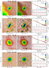 |
Fig. B.1. continued. |
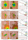 |
Fig. B.1. continued. |
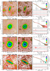 |
Fig. B.1. continued. |
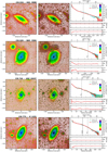 |
Fig. B.1. continued. |
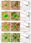 |
Fig. B.1. continued. |
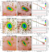 |
Fig. B.1. continued. |
All Tables
All Figures
|
Fig. 1. r-band images of the galaxy CIG 340 (IC 2487) from different surveys. Comparison between the Sloan Digital Sky Survey (left), the Legacy Survey (middle), and our data. The upper right value indicates the surface brightness limit [3σ, 10″ × 10″] of each image computed as explained in Sect. 2. The arrow in the left panel indicates the low surface brightness feature that is only visible in our data. |
| In the text | |
|
Fig. 2. Surface brightness image and profile of the galaxy CIG 340 (IC 2487). Left panel: r-band image. The scale of the colours represents the surface brightness of the image, and the scale is shown in the profile panel (right) following the y-axis scale. Middle panel: same image with the mask applied and the elliptical apertures of the dynamic position angle and ellipticity profile. Right panels: surface brightness profile (top), position angle (middle), and ellipticity (bottom) with respect to the radial distance in arcseconds (bottom) and kiloparsec (top). The red and green curves show the fit with dynamic and fixed elliptical apertures, respectively. The blue curve represents the fit with rectangular apertures. The position of the disc break (if any) is shown with the dashed elliptical aperture and the vertical dashed line in the middle and right panels, respectively. The dotted line in the right panel represents the radius at 25 mag arcsec−2. The figures for the whole sample of galaxies are given in Appendix B. |
| In the text | |
|
Fig. 3. Radii found via an automatic procedure as explained in Watkins et al. (2019) compared to those found via visual inspection of the profiles. The dotted grey line represents the 1:1 line, and the dashed orange line represents a linear fit to the data. The error bars were estimated using the distance to the next radial bins in the surface brightness profile at the distance at which the break was measured. |
| In the text | |
|
Fig. 4. Different examples of the interaction classification scheme. In the top panel, we show an unperturbed symmetric example (top left panel), CIG 100 (UGC 1863). The top middle and right panels show examples of perturbed galaxies. CIG 335 (NGC 2870) shows an overdensity in the halo region, and CIG 340 (IC 2487) shows a tidal stream in the southern region. All perturbation features are indicated with a black arrow. The bottom panels represent galaxies classified as cirrus-contaminated. CIG 1004 (NGC 7479), CIG 947 (NGC 7217), and CIG 154 (UGC 1706) are shown in the bottom left, middle, and right panels, respectively. These examples show considerable amounts of diffuse emission associated with Galactic cirrus only seen in our images. All of the images, except that of CIG 100, were smoothed with FABADA to enhance the structure. |
| In the text | |
|
Fig. 5. Frequency of the disc break type and the interaction signatures of our sample of galaxies. Left: normalised distribution of the frequency of the types of breaks found in this work (left, blue) and in Pranger et al. (2017) for their field (middle, green) and cluster (right, red) samples. Right: normalised distribution of the frequency of the types of breaks. Galaxies that are strongly contaminated by cirrus are excluded from this figure. We also show the contribution of unperturbed (blue) and perturbed (green) galaxies for each type of break. |
| In the text | |
|
Fig. 6. Photometric isolation parameter for 18 galaxies of our sample, and the local number density of neighbour galaxies, ηk, p, compared to the tidal strength, QKar, p, from Argudo-Fernández et al. (2013). The colour code represents the type of disc: blue, green, and red for Types I, II, and III, respectively. The mean values of each type are represented by the line close to the axis (bottom and left) with its corresponding error. Circles and stars represent unperturbed and perturbed galaxies, respectively. The mean values of perturbed and unperturbed galaxies are represented by the symbols close to the axis (upper and right) with their corresponding error. The crosses correspond to galaxies that were not classified due to galactic cirrus. Background grey values represent galaxies from different samples (see Sect. 4 for details). |
| In the text | |
|
Fig. B.1. Surface brightness images and profiles for all the galaxies in our sample. Left panel: r-band or luminance images for the galaxy. The ID of each galaxy is shown above. The scale of the colours represents the surface brightness of the image, and the scale is shown in the profile panel (right) following the y-axis scale. Middle panel: Same image with the mask applied and the elliptical apertures of the dynamic positional angle and ellipticity profile. Right panel: Surface brightness profile (top), positional angle (middle), and ellipticity (bottom) as a function of the radius in arcseconds (bottom) and kiloparsec (top). The red and green line show the dynamic and fixed elliptical apertures, respectively. The blue line represents the profiles obtained from rectangular apertures. The position of the disc break (if any) is shown with the vertical and elliptical aperture of the dashed line. The dotted line in the right panel represents the radius at 25 mag arcsec−2. We smoothed the CIG 613 image using the FABADA algorithm (Sánchez-Alarcón & Ascasibar 2023) to enhance the faint structures, and we indicate with arrows the tidal stream found for this galaxy. More information about the figure can be found in Section 4. |
| In the text | |
|
Fig. B.1. continued. |
| In the text | |
|
Fig. B.1. continued. |
| In the text | |
|
Fig. B.1. continued. |
| In the text | |
|
Fig. B.1. continued. |
| In the text | |
|
Fig. B.1. continued. |
| In the text | |
|
Fig. B.1. continued. |
| In the text | |
Current usage metrics show cumulative count of Article Views (full-text article views including HTML views, PDF and ePub downloads, according to the available data) and Abstracts Views on Vision4Press platform.
Data correspond to usage on the plateform after 2015. The current usage metrics is available 48-96 hours after online publication and is updated daily on week days.
Initial download of the metrics may take a while.