| Issue |
A&A
Volume 699, July 2025
|
|
|---|---|---|
| Article Number | A194 | |
| Number of page(s) | 19 | |
| Section | Interstellar and circumstellar matter | |
| DOI | https://doi.org/10.1051/0004-6361/202554109 | |
| Published online | 08 July 2025 | |
MINDS: The very low-mass star and brown dwarf sample
Detections and trends in the inner disk gas
1
Kapteyn Astronomical Institute, Rijksuniversiteit Groningen,
Postbus 800,
9700AV
Groningen,
The Netherlands
2
Max-Planck-Institut für Astronomie (MPIA),
Königstuhl 17,
69117
Heidelberg,
Germany
3
Leiden Observatory, Leiden University,
2300
RA
Leiden,
The Netherlands
4
Max-Planck Institut für Extraterrestrische Physik (MPE),
Giessenbachstr. 1,
85748
Garching,
Germany
5
Department of Astrophysics/IMAPP, Radboud University,
PO Box 9010,
6500
GL
Nijmegen,
The Netherlands
6
SRON Netherlands Institute for Space Research,
Niels Bohrweg 4,
2333
CA
Leiden,
The Netherlands
7
Institute of Astronomy, KU Leuven,
Celestijnenlaan 200D,
3001
Leuven,
Belgium
8
STAR Institute, Université de Liège,
Allée du Six Août 19c,
4000
Liège,
Belgium
9
Department of Planetary Sciences, University of Arizona; 1629 East University Boulevard,
Tucson,
AZ
85721,
USA
10
Niels Bohr Institute, University of Copenhagen,
NBB BA2, Jagtvej 155A,
2200
Copenhagen,
Denmark
11
Earth and Planets Laboratory, Carnegie Institution for Science,
5241 Broad Branch Road, NW,
Washington,
DC,
20015,
USA
12
Dept. of Astrophysics, University of Vienna,
Türkenschanzstr. 17,
1180
Vienna,
Austria
13
ETH Zürich, Institute for Particle Physics and Astrophysics,
Wolfgang-Pauli-Str. 27,
8093
Zürich,
Switzerland
14
Université Paris-Saclay, Université Paris Cité, CEA, CNRS, AIM,
91191
Gif-sur-Yvette,
France
15
Centro de Astrobiología (CAB), CSIC-INTA, ESAC Campus, Camino Bajo del Castillo s/n,
28692
Villanueva de la Cañada, Madrid,
Spain
16
INAF – Osservatorio Astronomico di Capodimonte,
Salita Moiariello 16,
80131
Napoli,
Italy
17
SRON Netherlands Institute for Space Research,
PO Box 800,
9700
AV,
Groningen,
The Netherlands
18
Department of Physics and Astronomy, University of Exeter,
Exeter
EX4 4QL,
UK
19
Space Research Institute, Austrian Academy of Sciences,
Schmiedlstr. 6,
8042
Graz,
Austria
20
TU Graz, Fakultät für Mathematik, Physik und Geodäsie, Petersgasse,
168010
Graz,
Austria
21
Université Paris-Saclay, CNRS, Institut d’Astrophysique Spatiale,
91405
Orsay,
France
★ Corresponding author: This email address is being protected from spambots. You need JavaScript enabled to view it.
Received:
12
February
2025
Accepted:
3
June
2025
Abstract
Context. Planet-forming disks around brown dwarfs and very low-mass stars (VLMS) are, on average, less massive and are expected to undergo faster radial solid transport than their higher-mass counterparts. Spitzer had detected C2H2, CO2, and HCN around these objects but did not provide a firm detection of water. With a better sensitivity and spectral resolving power than that of Spitzer, the James Webb Space Telescope (JWST) has recently revealed incredibly carbon-rich spectra and only one water-rich spectrum from such disks. A study of a larger sample of objects is necessary to understand how common such carbon-rich inner disk regions are and to put constraints on their evolution.
Aims. We present and analyze JWST MIRI/MRS observations of ten disks around VLMS from the MIRI guaranteed time observations program. This sample is diverse, with the central object ranging in mass from 0.02 to 0.14 M⊙. They are located in three star-forming regions and a moving group (1 to 10 Myr).
Methods. We identified molecular emission in all sources based on recent literature and spectral inspection, and reported detection rates. We compared the molecular flux ratios between different species and to dust emission strengths. We also compared the flux ratios with the stellar and disk properties.
Results. The spectra of these VLMS disks are extremely rich in molecular emission, and we detect the 10 μm silicate dust emission feature in 70% of the sample. We detect C2H2 and HCN in all the sources and find larger hydrocarbons, such as C4H2 and C6H6, in nearly all sources. Among oxygen-bearing molecules, we find firm detections of CO2, H2O, and CO in 90,50, and 20% of the sample, respectively. We find that the detection rates of organic molecules correlate with other organic molecules and anticorrelate with the detection rates of inorganic molecules. Hydrocarbon-rich sources show weaker 10 μm dust strengths, as well as lower disk dust masses (measured from millimeter fluxes) than the oxygen-rich sources. We find evidence for a C/O ratio enhancement with disk age. The observed trends are consistent with models that suggest rapid inward solid material transport and grain growth.
Key words: astrochemistry / protoplanetary disks / stars: low-mass / stars: pre-main sequence / infrared: planetary systems
© The Authors 2025
 Open Access article, published by EDP Sciences, under the terms of the Creative Commons Attribution License (https://creativecommons.org/licenses/by/4.0), which permits unrestricted use, distribution, and reproduction in any medium, provided the original work is properly cited.
This article is published in open access under the Subscribe to Open model. This email address is being protected from spambots. You need JavaScript enabled to view it. to support open access publication.
1 Introduction
Planets form around young stars from the dust and gas in the circumstellar disks. The physical and chemical properties of these disks vary with stellar mass and could directly affect the planet formation process. Infrared observations have revealed that disks surrounding the lowest-mass stars exhibit peculiar, carbon-rich gas compositions that differ greatly from those around higher-mass stars (Pascucci et al. 2009, 2013; Tabone et al. 2023; Arabhavi et al. 2024). These studies focus on disks around central objects with masses up to 0.15 solar masses, which we refer to as very low-mass stars (VLMS). Planet population synthesis models and observations indicate that rocky planets have the highest occurrence rates around objects with masses much lower than those of Sun-like stars (Burn et al. 2021; Sabotta et al. 2021). This makes the study of VLMS disks very interesting for understanding the formation of rocky planets. The composition of the inner regions of these disks can provide strong constraints on the composition of the planets that form around such stars.
Disks around VLMS differ from those around higher mass T Tauri stars in several ways. Due to their low disk masses and stellar luminosities, the ice lines in the VLMS disks are located much closer to the star (Pascucci et al. 2016; Greenwood et al. 2017). For example, models show that the water and CO ice lines around a typical T Tauri disk are at about 1 and 20 au, respectively (Kamp et al. 2017), while the same ice lines around a typical VLMS are at about 0.1 and 2 au (Greenwood et al. 2017). Due to such small distances between ice lines and the very short dynamic timescales in the VLMS disks (Pinilla et al. 2013; van der Marel & Pinilla 2023), the radial transport processes have more significant impact on their disk composition compared to T Tauri disks (Mah et al. 2023). Observations, such as those from the Hubble Space Telescope (Manara et al. 2012) and the Very Large Telescope (Fedele et al. 2010), show that the accretion rates in VLMS disk systems fall off quickly by several orders of magnitude within a few million years, whereas those in the T Tauri disks decrease much slower. Observations also show that the disks around VLMS have, in general, weaker silicate dust features compared to the higher-mass counterparts, indicating more efficient grain growth (Apai et al. 2005; Pascucci et al. 2009). Furthermore, the properties of the central objects also differ significantly in terms of their stellar activity, X-ray luminosity, temperature, and stellar spectral energy distribution (Güdel et al. 2007; Basri et al. 2000; White & Basri 2003; Luhman 2012; Rice et al. 2010).
Spitzer Infrared Spectrograph (Spitzer-IRS) observations (Pascucci et al. 2009, 2013) of the inner regions of the VLMS disks (≲0.1 au from the central object, Kessler-Silacci et al. 2007) have shown an underabundance of HCN relative to C2H2 when compared to the inner disks of the higher-mass counterparts (≲1 au from the central object) and only tentative detections of water in two young disks in the Taurus star-forming regions (SFRs). Observations with the higher resolution and sensitivity of the Mid-InfraRed Instrument (MIRI) on the James Webb Space Telescope (JWST) have enabled detailed characterizations of the VLMS, revealing a rich hydrocarbon chemistry including isotopologues of some species (Tabone et al. 2023; Arabhavi et al. 2024; Kanwar et al. 2024a; Morales-Calderón et al. 2025). These objects generally show strong hydrocarbon emission and sometimes even hydrocarbon molecular pseudo-continua but do not show firm detections of water or OH, indicating the C/O ratio is larger than unity in the emitting regions (Tabone et al. 2023; Arabhavi et al. 2024). Xie et al. (2023) reported a water-rich disk around the source Sz 114 (M* = 0.17 M⊙) and suggest that this source could be at an early evolutionary stage compared to the other VLMS disks, while Long et al. (2025) presented a very carbon-rich MIRI spectrum of a 30 Myr old VLMS disk. Perotti et al. (2025) present a MIRI spectrum of a highly inclined brown dwarf disk, which appears to be water-rich. More recently, Flagg et al. (2025) reported a hydrocarbon-rich disk around a planetary-mass object (<0.01 M⊙) with a MIRI spectrum remarkably similar to the VLMS disk presented by Arabhavi et al. (2024).
Two scenarios are proposed to explain the hydrocarbon-rich inner disk (Tabone et al. 2023; Mah et al. 2023; Arabhavi et al. 2024): (i) carbon enrichment through carbon grain destruction and (ii) oxygen depletion by disk transport processes or dust traps. In the former, the carbon trapped in the dust is released to the gas phase by sublimation, combustion, chemosputtering, or photoprocesses, leading to a carbon-rich gas in the inner disk. In the latter, efficient transport processes in these VLMS disks (Pinilla et al. 2013) can lead to early preferential accretion of the oxygen-bearing molecules onto the central object, fed by the oxygen-dominated ices in the midplane beyond the snowline (Mah et al. 2023). This would lead to an oxygen-depleted gas in the inner disk over time. In both of these scenarios, the enhanced C/O gas composition (C/O>1) leads to the efficient formation of hydrocarbons either in the gas phase (Kanwar et al. 2024a) or on grain surfaces (provided suitable dust temperatures) (Woods & Willacy 2007; Henning & Krasnokutski 2019).
Inner disk substructures can influence the local chemical compositions and play an important role in explaining the observed infrared spectra of such sources. Kalyaan et al. (2023), Mah et al. (2024), Lienert et al. (2024), and Sellek et al. (2025) show that the nature of the gaps, particularly whether the gaps are due to pebble traps, planets, or photoevaporative winds, can strongly influence the inner disk elemental composition. Kanwar et al. (2024b) carry out thermochemical modeling introducing a gap that splits the disk into a high C/O inner disk and a more normal outer disk and can reproduce the observed JWST carbon-rich spectrum, including pseudo-continuum and CO2 emission in the absence of strong water emission.
Due to low disk masses, luminosities, and small spatial scales, there is a lack of spatially resolved observations of the inner disks of these systems. Deeper and more extensive studies, such as with the Atacama Large Millimeter/submillimeter Array (ALMA), should be used to provide more detailed information for the brighter VLMS disks.
In this paper, we present and analyze the JWST MIRI spectra of disks around ten VLMS, focusing on gas detections. Arabhavi et al. (2025) provide a detailed discussion on detections of water in the sample. We present the sample, the observations, and the data reduction process in Sect. 2. We discuss the molecular detections and the detection rates in Sect. 3. In Sects. 4 and 3.2, we present trends observed in the molecular flux ratios and notes on individual sources, respectively. The implications of our findings are discussed in Sect. 5, and finally, the conclusions are presented in Sect. 6.
2 The sample, observations, and data reduction
2.1 The sample
The observations are part of the MIRI midINfrared Disk Survey (MINDS) program, a JWST guaranteed time observations (GTO) program (ID: 1282, PI: Th. Henning, Henning et al. 2024; Kamp et al. 2023). This GTO program includes 10 VLMS sources, of which nine have been observed and are presented in this work (see also Tabone et al. 2023; Arabhavi et al. 2024; Kanwar et al. 2024a; Perotti et al. 2025; Morales-Calderón et al. 2025). We also include a brown dwarf disk, TWA27A (further referred to as TWA27), from the exoplanet GTO program (PID: 1270; PI: S. Birkmann; see also Patapis et al. in preparation). The properties of the sample are summarized in Table 1. The spectral type of the sources ranges from M4.5 to M9. These sources are located in three SFRs – Taurus, Chamaeleon, and Upper Sco – and one moving group, the TW Hydrae Association. Some of the sources have high visual extinction values (e.g., Av=4.8 mag for NC9; see Table 1). One of the sources, J0438, is a highly inclined disk (~70°, Scholz et al. 2006; Luhman et al. 2007). All of the sources in our sample were previously observed with Spitzer-IRS (Riaz & Gizis 2008; Pascucci et al. 2009, 2013). The spectra showed both dust features and gas emission lines. Table 1 summarizes the molecular and atomic emissions detected with Spitzer. All sources were observed with ALMA in the continuum at 0.89 mm (Pascucci et al. 2016; Barenfeld et al. 2016; Ricci et al. 2017; Ward-Duong et al. 2018), except NC1 for which the observation failed. In these observations, IC147, Sz28, and J1605 were not detected. The estimated dust masses (or the upper limits) are listed in Table 1. Only J0438, J1558, and TWA27 were firmly detected in millimeter gas emission in the 12CO J = 3–2 line with ALMA (Barenfeld et al. 2016; Ricci et al. 2017; Perotti et al. 2025). 1.3 mm continuum observations have been performed with the IRAM 30 m single-dish telescope and the Submillimeter Array (SMA) telescope for the two Taurus sources and with ALMA for J0438 (Andrews et al. 2013; Scholz et al. 2006; Ward-Duong et al. 2018). Compared to their higher-mass counterparts, the VLMS disks are smaller and fainter, which limits their observability.
2.2 Observations
The sources were observed with the MIRI (Rieke et al. 2015; Wright et al. 2015, 2023) of JWST with the Medium Resolution Spectroscopy (MRS; Wells et al. 2015; Argyriou et al. 2023) mode. This involves four integral field units (IFUs): channel 1 (4.9–7.65 μm), channel 2 (7.51–11.71 μm), channel 3 (11.55–18.02 μm), and channel 4 (17.71–27.9 μm), and each channel is composed of three sub-bands: SHORT (A), MEDIUM (B), and LONG (C), leading to a total of twelve wavelength bands. The sources were observed with target acquisition and were observed in FASTR1 readout mode with a four-point dither pattern in the positive direction, for a total exposure time per sub-band per source of ~1232 s. TWA27, however, was observed with the extended source four-point dither pattern in the negative direction for a total exposure time per sub-band of ~844 s.
Summary of the source properties.
2.3 Data reduction
We used a hybrid pipeline (v1.0.3, Christiaens et al. 2024) relying on the standard JWST pipeline (v1.14.1, Bushouse et al. 2023) using CRDS context (jwst_1254.pmap file), and complemented with routines from the VIP package (Gomez Gonzalez et al. 2017; Christiaens et al. 2023), to reduce the data. The pipeline is structured around three main stages that are the same as in the JWST pipeline, namely Detector1, Spec2, and Spec3. After the first stage (Detector1), stray light is corrected, and a background estimate is subtracted. To remove the background, we carried out a direct pair-wise dither subtraction. This method is more suited to fainter sources (which is the case for all our VLMS sources), where the resulting PSF overlap is minimal and reduces the noise level in the spectrum but can lead to a minor flux discrepancy with prior Spitzer measurements due to self-subtraction (this minor discrepancy will not affect our analysis in this work). Since TWA27 was observed in an extended source dither pattern, the half-integral dither offset leads to self-subtraction while using the direct dither subtraction to remove the background. This results in a drop in flux in the final spectrum. We compared this with the spectrum obtained by measuring the background in an annulus around the source. The latter is noisier, but matches well with the flux levels reported with Spitzer. We used the flux levels from the annulus to rescale the less noisy spectrum obtained from direct dither subtraction. This does not affect the relative or absolute molecular and dust flux levels. Spec2 was then used with default parameters, but the stray light correction and background subtraction were skipped.
The outlier detection step in Spec3 was skipped, and replaced by a custom VIP-based bad pixel correction routine applied before Spec3. The bad pixels were identified through sigma-filtering and corrected with a Gaussian kernel. This significantly reduced the number of spikes otherwise present in the spectra extracted with early versions of the official JWST pipeline1. The VIP-based routines were then also used for the identification of the star centroid in the spectral cubes produced at stage 3. The centroid location was identified with a 2D Gaussian fit in a weighted mean image for each band’s spectral cube, where the weights were set to be proportional to each frame’s integrated flux in the central part of the field. The identified centroid locations were subsequently used for aperture photometry: the spectrum was extracted by summing the signal in a 2×FWHM aperture centered on the source, where the FWHM (full width half maximum) is equal to 1.22 λ/D, with λ the wavelength and D ~ 6.5m the diameter of the telescope. Aperture correction factors were applied to account for the flux loss as presented in Argyriou et al. (2023).
For the analysis of the spectra, we required molecular fluxes, i.e., line fluxes above the dust continuum. For this, we determined the continua using the procedure described in Temmink et al. (2024), which uses the pybaselines package (Erb 2022). This allows for a reproducible continuum definition instead of tracing the dust emission by eye. The method first estimates a continuum level using Savitzky-Golay filter and masks strong line emission above 2σ. Furthermore, Temmink et al. (2024) mask the 3σ downward spikes. The VLMS spectra are generally line-rich and can show molecular pseudo-continuum emission. This leads to difficulties in (1) distinguishing between broad dust continuum features and molecular continuum and (2) identifying the dust continuum level to mask the downward spikes. So, we skipped the masking of the downward spikes. We defined two continua for each source, corresponding to broad and narrow widths of the Savitzky-Golay filter. Subtracting the continuum defined with the narrow width subtracts the dust (including the optically thin dust features) as well as the molecular pseudo-continuum, while the broad width continuum retains the broad features. The latter was used to measure the dust strengths and the molecular fluxes in case of molecular pseudo-continuum. More details on the continuum definition method can be found in Sect. 2.2 of Temmink et al. (2024). The final reduced spectra, and comparison with the Spitzer spectra are presented in Appendices A and B.
2.4 Extinction
The spectra are affected by extinction along the line of sight. The extinction estimates based on ultraviolet (UV), visible and near-infrared spectroscopy presented by Herczeg & Hillenbrand (2008), Herczeg & Hillenbrand (2014), Manara et al. (2016), and Manara et al. (2017) are listed in Table 1. J0438 is a highly inclined disk whose extinction estimate is expected to be largely influenced by its high inclination (>70°, Scholz et al. 2006), but also by any foreground extinction. Hence, the reported value (Av=2.8 mag) for J0438 should be taken as an upper limit.
For the remainder of this study, we de-reddened the spectra using the extinction law from Gordon et al. (2023) (which relies on Gordon et al. 2009; Fitzpatrick et al. 2019; Gordon et al. 2021; Decleir et al. 2022) using the dust_extinction python package (Gordon 2024). A comparison of the spectra before and after de-reddening is presented in Appendix A. Since most of the molecular emission analyzed in this paper occurs in a narrow wavelength range, well separated from the silicate features, the accuracy of the extinction values and the extinction curves does not affect our conclusions.
3 Detections and detection rates
The MIRI spectra of our sample show several molecular emission bands along with dust features of varying strengths. The detection criteria and detection of individual species in each source are provided in Appendix C. Here, we summarize the detections and the detection rates.
3.1 Detection rates
Figure 1 provides an overview of the dust and gas features. The left panels show the continuum-normalized dust strengths of the optically thin emission. Seven sources (J0438, J0439, J1558, NC9, NC1, HKCha, and Sz28) show prominent silicate emission (Fig. 1), while the remaining three sources (J1605, TWA27, IC147) show almost flat 10 μm regions. IC147 shows a shallow feature with a peak at ~10 μm whose shape is quite distinct from the rest of the detected dust features. Moreover, Arabhavi et al. (2024) show that emission from a large column density of C2H4 can reproduce the broad shape before de-reddening.
In general, the observed 10 μm dust shapes are flat-topped and weaker than those observed in the T Tauri disks (see also Grant et al., in preparation), in-line with previous Spitzer observations (Apai et al. 2005, Kessler-Silacci et al. 2007). We find peaks at ~9.2 μm corresponding to SiO2 and/or enstatite and 11.3 μm corresponding to forsterite. A more detailed analysis of these dust features will be presented in Jang et al. (in prep). In this paper, we focus on the gas composition of these inner disks.
All of the sources are rich in gas species, as shown in the middle and right panels in Fig. 1. C2H2 and HCN are ubiquitously detected across all the sources due to the better sensitivity of JWST, compared to detection rates of 41 and 22%, respectively, deduced from Spitzer spectra (Pascucci et al. 2009, 2013). CO2 is detected in all sources with the exception of J1558, in which the detection is tentative (Fig. C.3). Considering the entire sample, we detect H I, [Ar II], [Ne II], H2, OH, H2O, CO, CO2, HCN, HC3N, CH3, CH4, C2H2, C2H4, C2H6, C3H4, C4H2, and C6H6, along with two isotopologues – 13CO2 and 13CCH2. Consistent with the Spitzer findings (e.g., Pascucci et al. 2009), the HCN fluxes are typically weaker than the C2H2 fluxes. The VLMS sample studied by Pascucci et al. (2013) with Spitzer showed a [Ne II] detection rate of 2/8, while it is only 1/10 in our sample. Pascucci et al. (2013) reported a tentative detection of [Ne II] in J0439, but we do not detect [Ne II] in the MIRI spectrum.
Figure 2 summarizes the detections and detection rates of different species. The lower left panel shows the emission features detected in each source. The top panel shows the detection rates of organic molecules in light red and inorganic molecules in gray. In general, these spectra are rich in organic molecules. If we include the tentative detections, more than 50% of the detected molecules are purely hydrocarbons, and more than 80% contain carbon. While we detect the hydrocarbons such as C2H2, C4H2, and C6H6 in 10,9, and 8 sources in the sample of 10 objects, we detect oxygen-bearing molecules such as CO2, H2O, and CO in 9, 5, and 2 sources, respectively (see Arabhavi et al. 2025 for a more detailed discussion on detections of water in the sample). H2 and H2O are the most commonly detected non-carbon-bearing molecules. C2H4 is the least commonly detected organic molecule (only TWA27 and IC147). While three sources (J0438, J1558, J1605) show H I, H2, and H2O emission simultaneously, CO is detected only in the two Upper Sco objects, J1605 and J1558. Except for J1605, J1558, and NC1, all the other sources are dominated by the stellar photospheric absorption of CO and H2O at shorter wavelengths (≲7 μm). Across the sample, benzene (C6H6) is the only aromatic hydrocarbon detected, and we do not find any polycyclic aromatic hydrocarbons (PAHs) in these spectra.
3.2 Notes on spectral appearance
J0438: It is a highly inclined disk with a peculiar 10 μm shape showing dust in both absorption and emission. The MIRI spectrum appears water-rich, closer to T Tauri spectra in appearance (water was tentatively detected in its Spitzer spectrum, Pascucci et al. 2013). C2H2 is the only hydrocarbon detected, and the CO2 flux is also weaker than many water lines. This is the only source where [Ne II] and [Ar II] are detected (see Perotti et al. 2025 for a full discussion on this source).
J1558: It is a C2H2-bright source. The continuum-subtracted peak flux of C2H2 is ~22.2 mJy, which is almost identical to the peak flux of C2H2 in the J1605 spectrum (both are UpperSco sources; see Fig. 1). However, the 13CCH2 feature is absent or very weak, implying that C2H2 in J1558 has column densities at least an order of magnitude lower than what is reported for J1605 (Tabone et al. 2023). Such bright emission at low column densities requires a large emitting area or high temperature. The J1558 spectra is also water-rich, but surprisingly CO2 is absent or very weak. This is opposite to what is observed in the rest of the sample, where CO2 is more readily detectable than water.
J0439: This is the only source where we clearly detect several organic molecules as well as rotational water lines.
NC1: This source has the strongest 10 μm dust feature. The dust feature shape resembles closely some of the T Tauri disks. Figure 3 compares the dust feature with SY Cha (Schwarz et al. 2024). While this source shows infrared excess and rovibrational water emission shortward of 8 μm, CO emission is undetected. This source also shows emission from several organic molecules (see Morales-Calderón et al. 2025 for more details).
NC9, HKCha, and Sz28: These sources have similar dust shapes and strengths but differ in terms of their molecular detections.
J1605: This source has one of the brightest C2H2 emission strengths in a VLMS disk, and C2H2 is extremely optically thick (Tabone et al. 2023). It also has the flattest 10 μm region of all our spectra without an optically thin dust feature. The number of organic molecules detected in J1605 is smaller than in many other sources in our sample.
TWA27 and IC147: These two sources show the largest number of organic molecules in emission. The overall shape of the MIRI spectra are also similar. The two sources show emission from C2H4, which coincides with the 10 μm dust feature. It is not fully clear whether the broad shapes at these wavelengths are entirely C2H4 or partly due to dust.
 |
Fig. 1 Summary of dust and gas observations. The left panels show continuum-normalized dust strengths highlighting SiO2, enstatite, and forsterite emission features. The middle panels present a close-up of the observed C2H2 features, highlighting four peaks corresponding to the main and rare isotopologues in red and blue, respectively. The right panels show the continuum-subtracted hydrocarbon-rich wavelength region of the spectra. The gray regions highlight the main Q branches of molecules in this wavelength region. HCN* and |
![Mathematical equation: $\[\mathrm{CO}_{2}^{*}\]$](/articles/aa/full_html/2025/07/aa54109-25/aa54109-25-eq1.png)
3.3 Correlations and anticorrelations in detection rates
The right panel of Fig. 2 shows the number of organic and inorganic molecules detected in each source. The number of organic molecules detected in most sources is much larger than that of inorganic molecules. Exceptions to this are the highly inclined disk J0438 and the C2H2-bright disk J1558.
A quantitative measure of the trends in the gas detections can be obtained by calculating correlation coefficients. The right panel of Fig. 2 shows that the number of organic and inorganic molecules detected in each source are anticorrelated, with a Pearson correlation coefficient of −0.78 (p-value 0.007). Figure D.1 shows the binary correlation coefficients ϕ (Yule 1912) and the p-values between the species detected in the sample. A strong correlation between a molecule pair implies that it is more probable for the two molecules to be either detections or non-detections. On the other hand, an anticorrelation between a molecule pair implies that it is more probable that only one of the molecules is detected at a time. Less dominant (relative to C2H2) organic molecules such as C3H4, C2H6, and HC3N are strongly correlated (see Fig. 4). Inorganic molecules such as H2 and H2O are anticorrelated with the organic molecules. Since CO2 is detected in all sources, it is not surprising to find that 13CO2 also correlates with organic molecules (Fig. D.1).
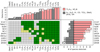 |
Fig. 2 Summary of dust and gas detections in the sample. The green square refers to a firm detection, the yellow square indicates a tentative detection, and the light gray square indicates a non-detection. The top panel shows the number of detections for each species. The right panel shows the number of species of two groups detected in each source. The inorganic species (dark gray) include H2, H2O, HI, CO, CO2, 13CO2, [Ne II], and OH. The organic species (faded red) include all the hydrocarbons and cyanomolecules. The hatched region in the top and right panels shows tentative detections. |
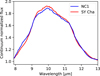 |
Fig. 3 Comparison of the 10 μm dust feature of NC1 (VLMS) and SY Cha (T Tauri). Here the continuum-normalized flux is shown. The observed MIRI spectrum of SY Cha is taken from Schwarz et al. (2024). |
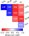 |
Fig. 4 Binary correlation coefficients between the detection rates of a few species with strong (anti)correlations. Correlation coefficients (and the p-values) for a more extended list of species are shown in Fig. D.1. |
4 Trends in the sample
4.1 13CCH2 to C2H2 flux ratio as a measure of column density
Estimating the column densities, temperatures, and emitting radii of the molecules using OD slab models2, as done with Spitzer observations, would be beneficial for a quantitative analysis. However, several molecular features observed in the spectra cannot be reproduced by models due to the lack of molecular data (e.g., Tabone et al. 2023; Arabhavi et al. 2024; Kanwar et al. 2024a). In addition, studies of JWST observations of disks around VLMS such as Tabone et al. (2023) and Arabhavi et al. (2024) have shown that the fitting procedure is not trivial for these rich spectra due to spectral overlap of multiple molecules. Moreover, a single 0D model might not be able to reproduce the observed molecular features. Analysis using more sophisticated tools such as 1D retrieval tools (e.g., CLIcK – Liu et al. 2019, DuCKLinG – Kaeufer et al. 2024a,b) is left to a future work. Consequently, we limit ourselves to the analysis using the integrated line fluxes in this work. Furthermore, the spectra are rich in molecules, and the molecules individually emit in a very large wavelength range, which makes estimating the total flux of a molecule impossible without performing slab model fits. Therefore, we rely only on the fluxes of the Q-branches for the rest of the analysis.
The middle panels in Fig. 1 show a close-up of the C2H2 features of the sample. We identify four peaks:
13.679 μm C2H2 - v4 + v5: 1, 1 − 1, 0
13.691 μm 13CCH2 - v4 + v5: 1, 1 − 1, 0
13.712 μm C2H2 - v5: 1 − 0
13.730 μm 13CCH2 - v5: 1 − 0.
The relative strengths of these peaks exhibit considerable diversity across the sample. The width at the base also varies. Each peak mentioned above is a band head with a tail toward the shorter wavelengths, which results in flux contributions of each band to the remaining peaks at the shorter wavelengths. Peaks 3 and 4 are the least contaminated peaks corresponding to the primary and secondary isotopologue of C2H2 whose integrated fluxes (between 13.698–13.723 μm, and 13.723–13.734 μm, respectively) will be referred to as FC2H2 and F13CCH2 in the rest of the paper. The sources in Fig. 1 are ordered according to the ratio of these fluxes (F13CCH2/FC2H2).
As the gas column density increases, the optical depth also increases. Consequently, at high gas column densities, the integrated flux FC2H2 saturates. Assuming that the isotopologue 13CCH2 emits from the same region as C2H2, the abundance of the isotopologue 13CCH2 is expected to be lower by a factor of 1/35 than that of C2H2 (assuming the interstellar 12C/13C ratio of ~70, Woods & Willacy 2009), which makes it optically thinner. Therefore, the peak associated with that, F13CCH2, is less saturated at those high column densities. If the C2H2 and 13CCH2 gas columns extend below the optically thick τC2H2=1 surface, F13CCH2 continues to increase with the increasing column density before saturation. Assuming that the isotopic fractionation of carbon is uniform across the disk, the F13CCH2/FC2H2 ratio would be least affected by the radial extent of the hydrocarbon emission. However, the flux ratio would strongly reflect the vertical gas composition above the optically thick dust layer (the depth of this dust layer would be determined by the dust size distribution and dust settling). We can leverage the ratio of the integrated fluxes of these two peaks as a measure of the column density or the gas optical depth probed by MIRI. Since we expect to probe large column densities of C2H2 and 13CCH2, we also expect a large contribution of higher excited bands to the Q-branch peaks. Due to the unavailability of spectroscopic data of 13CCH2 beyond the fundamental band, a quantitative analysis of the observed fluxes to determine column densities is not feasible. Qualitatively, a higher value of F13CCH2/FC2H2 indicates a larger column density of gas being probed.
While we assume uniform isotopic fractionation of carbon in the case of C2H2 and 13CCH2, preferential shielding from UV radiation, or chemical fractionation could lead to deviations in the local 12C/13C ratio. In such cases, the range of F13CCH2/FC2H2 ratios and the related trends (Sects. 4.2 and 4.3) reported for our sources could be partly due to these fractionation processes.
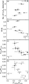 |
Fig. 5 Trends in the MIRI observations. Panels A-D show the number of hydrocarbons (CnHm) detected, the integrated dust strength, the CO2 to C2H2 flux ratios, and the H2O to C2H2 flux ratios against the flux ratio F13CCH2/FC2H2, along with the error bars. The molecules with tentative or non-detections are indicated by the upper limits. In case of non-detections, we report the 1σ upper limits. All error bars are 1σ with an assumption of a S/N of 100. |
4.2 Trends in the MIRI observations
In Fig. 5, we investigate the detection rate of organic molecules, the dust strengths, and the molecular flux ratios as a function of F13CCH2/FC2H2. Using the JWST Exposure Time Calculator3 and adopting the same observational setup – including the MIRI exposure times – as used for our observations, we estimate signal-to-noise ratios (S/Ns) ranging from 100 to 270 in the wavelength regions where the line fluxes are measured, based on the observed flux levels. To be conservative, we choose the lower limit of the S/N range (=100) for the error bars and upper limits. More details on the S/N estimation are discussed in Jang et al. (in prep.). We do not include J0438 because it is highly inclined, and the F13CCH2I/FC2H2 ratio would have large error bars.
4.2.1 Number of hydrocarbon species detected
Except for J1605, a higher F13CCH2/FC2H2 ratio corresponds to a larger number of hydrocarbons detected (panel A of Fig. 5). This is very likely because the higher F13CCH2/FC2H2 ratios correspond to large columns of gas being probed, or equivalently, higher gas optical depths. A large column of gas could allow sufficient column densities of less abundant hydrocarbons to be present in the line of sight such that their emission is above the noise level. This can explain the strong correlations between the detection rates of less dominant hydrocarbons such as C3H4 and C2H6 (Figs. 4 and D.1). However, J1605 appears to be an outlier, which has a large F13CCH2/FC2H2 ratio but only about half the number of organic molecules as detected in other sources with similar flux ratios. Furthermore, when F13CCH2/FC2H2>0.3, the only inorganic molecule detected is CO2 (and 13CO2), while in J1605, CO, H2O, H2, and H I have been detected in addition to CO2.
4.2.2 Dust strengths
Generally, the dust opacity limits the depth that can be probed in disks at infrared wavelengths. Due to efficient grain growth, VLMS disks are expected to have larger dust grain sizes (Apai et al. 2005) and consequently lower infrared dust opacities than their higher-mass counterparts. The lower dust opacities can allow infrared emission to probe deeper layers of the disk and thus larger columns of gas (e.g., Antonellini et al. 2015). The left and middle columns of panels in Fig. 1 show the spectral appearance of the dust and the C2H2 features ordered by the F13CCH2/FC2H2 ratio. We observe a general trend of higher gas optical depths probed in sources with lower dust strengths (F9.8, the continuum-normalized dust strength at 9.8 μm; panel B of Fig. 5). However, there is some scatter. For example, NC1 has the strongest dust feature, but it does not necessarily have the smallest flux ratio. This could be due to several factors, such as the infrared dust and molecular emission arising from slightly different disk regions.
4.2.3 Water and CO2
As discussed in Sect. 3, the water detections anticorrelate with some of the organic molecules (Fig. 4). FCO2 is the integrated line flux of CO2 between 14.920 μm and 14.993 μm, and FH2O is the sum of the integrated line fluxes of three water lines at 16.66, 17.10, and 17.36 μm (16.654–16.673, 17.092–17.112, 17.354–17.363 μm, respectively). While there is likely underlying hydrocarbon emission, we do not identify strong hydrocarbon Q–branch emission at these wavelengths. Thus, non-detections provide upper limits on H2O line fluxes. At even longer wavelengths, the VLMS disks are very faint, and the sensitivity of MIRI also decreases, leading to high noise levels.
In general, we observe that for sources in which we probe deeper columns of gas, the CO2 and H2O emissions are weaker relative to C2H2 (panels C and D of Fig. 5, respectively). Since CO2 is detected in more sources than H2O, this trend is more evident in panel C. The large scatter in panel D is likely due to the underlying hydrocarbon emission at the wavelengths where the water flux is measured. The Q-branch emission of CO2 in panel C is less affected by the hydrocarbon emission, as demonstrated by Arabhavi et al. (2025). The flux ratios for the source J1558 are outliers. This is because J1558 is distinctly bright in C2H2 (as bright as J1605; see Fig. 1) but hydrocarbon-poor, unlike most of the sources in our sample (see Sect. 3.2). The observed trend of relative decrease in CO2 and H2O fluxes could be due to (i) lower abundances of these oxygen-bearing molecules, or (ii) the hydrocarbon fluxes are more sensitive to increasing column density than CO2 and H2O (see Sect. 5 and Arabhavi et al. 2025).
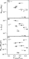 |
Fig. 6 Trends in stellar and disk properties. Panels A-C show the dust mass (estimated from 0.89 mm continuum fluxes), stellar luminosity, and mass accretion rate against the flux ratio F13CCH2/FC2H2. |
4.3 Trends in stellar and disk properties
While mid-infrared wavelengths probe the inner disks, millimeter wavelengths probe the outer disk. Since dynamic processes, such as radial material transport, affect both the inner and outer disks, we compare the 13CCH2-C2H2 flux ratios of the inner disks with ALMA continuum fluxes, which probe the outer disk dust masses. We also investigate relations with the stellar luminosity and the mass accretion rates.
Panel A of Fig. 6 shows the dust masses calculated from ALMA 0.89 mm fluxes (from Manara et al. 2023, Ricci et al. 2017) using the optically thin dust prescription of Manara et al. (2023) (Table 1). The dust mass decreases with higher flux ratios, indicating that disks with larger columns of hydrocarbons have lower pebble masses in the outer disk. A similar trend is also observed with stellar luminosity (panel B), where the gas optical depth probed by F13CCH2/FC2H2 ratio increases with lower stellar luminosity. Arabhavi et al. (2025) show that the observed peak-to-continuum ratio of C2H2 increases with decreasing stellar luminosity. These findings point to a larger column of gas probed in disks around less luminous objects. This is in line with the non-detections of 13CCH2 in all T Tauri disk spectra published so far (e.g., Grant et al. 2023), except one (Colmenares et al. 2024). No clear trend is observed with mass accretion rates (panel C).
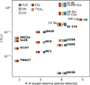 |
Fig. 7 Luminosities of the central object against oxygen-bearing molecules in the inner disks. The colored boxes refer to the oxygen-bearing molecules detected in the MIRI spectra of each source, indicated in the legend. Tentative detections are highlighted by white crosses. The VLMS disks are highlighted in bold. The detection in T Tauri disks are taken from the following papers: GW Lup (Grant et al. 2023), Sz 98 (Gasman et al. 2023), DR Tau (Temmink et al. 2024), SY Cha (Schwarz et al. 2024), CX Tau (Vlasblom et al. 2025), and V1094Sco (Tabone et al. in prep.). Detections of Sz114 are obtained from Xie et al. (2023). |
4.4 Oxygen carriers at mid-infrared wavelengths
Figure 7 shows the stellar luminosity against the number of oxygen-bearing molecules observed in the inner disks. For comparison, we include six T Tauri disks from the MINDS sample (GW Lup, Sz 98, DR Tau, SY Cha, CX Tau, and V1094Sco) and one additional VLMS disk (Sz 114). In general, the more luminous objects – and thus the T Tauri disks – show a greater diversity of oxygen-bearing molecules compared to less luminous objects. While H2O, OH, CO, and CO2 are the most commonly detected oxygen-bearing molecules in the T Tauri disks, 13CO2 is detected only in sources known to be CO2-bright (i.e., in sources with weaker H2O emission); for example, see Grant et al. (2023) and Vlasblom et al. (2025). On the other hand, in the VLMS disk sample, CO2 and 13CO2 are the most commonly detected oxygen-bearing molecules, while CO emission is observed only in the two Upper Sco objects. Although the VLMS disks generally have lower detection rates of oxygen-bearing molecules compared to the T Tauri disks, all sources show emission from at least two oxygen-bearing molecules (including the isotopologues). See Arabhavi et al. (2025) for a more detailed discussion on oxygen-bearing molecules, particularly water, in VLMS disks. See Grant et al. (in preparation) for a more detailed comparison of VLMS and T Tauri disk samples.
5 Discussion
The evolution path toward an enhanced C/O gas composition can follow rapid inward material transport, carbon grain destruction, or H2O-ice trapping in the outer disk. These scenarios leave distinct signatures on the gas and dust compositions that can be probed at infrared and millimeter wavelengths.
In the rapid inward material transport scenario, Mah et al. (2023) predict that the volatile C/O would decrease initially (within ~0.5 Myr). Later, the C/O would rapidly increase with the age of the disk, and this enhancement is faster in disks around less massive stars than their higher-mass counterparts. Dynamic disk models such as Pinilla et al. (2013) suggest that VLMS disks experience rapid grain growth along with rapid inward material transport.
Carbon grain destruction is also expected to enhance the C/O in the disk. However, this process can occur even in disks around higher-mass stars and is not clear why it would be limited to only VLMS disks. This process does not necessarily require rapid inward material transport but can occur simultaneously and further enhance the C/O.
Kalyaan et al. (2023) and Mah et al. (2024) show that, in T Tauri disks, deep gaps can limit the delivery of oxygen-bearing ices to the inner disk and lead to a high C/O in the inner disk within a few million years. Trapping of material in the outer disk could result in brighter outer disks compared to disks with efficient radial dust transport. In line with this, Kanwar et al. (2024b) show that a thermochemical model with a gap close to the H2O ice line that separates an oxygen-depleted (high C/O) inner disk and normal outer disk can reproduce the MIRI spectrum of the hydrocarbon-rich disk of J1605.
5.1 Tentative evidence for C/O enhancement with age
The evolution timescales of the VLMS disks are expected to be short. Moreover, during this evolution, the stellar luminosities are also expected to decrease. The age of the individual objects is not available, but we find that sources with lower stellar luminosities show higher F13CCH2/FC2H2 ratios (and are possibly more carbon-rich, Fig. 6).
Although the age of individual objects is not well constrained, the typical age of their SFRs or moving groups can provide some insights into the evolution of these objects. Figure 8 shows the flux ratio of the isotopologues of the predominant oxygen and carbon carriers in the spectra (F13CO2/F13CCH2) versus the flux ratio of the predominant carriers themselves (FCO2/FC2H2). The trend is very close to the line with a slope of unity in the log-log scale. This can be explained by the ISM fractionation ratio of 12C/13C~70 (Woods & Willacy 2009); neglecting the optical depth effects, F13CO2/F13CCH2 = 0.5 · FCO2/FC2H2, or log10(F13CO2/F13CCH2) = log10 (0.5) + log10 (FCO2/FC2H2). We do not capture the offset of log10 (0.5) in Fig. 8 because we show here only the integrated fluxes around the peaks and not the entire molecular flux. Interestingly, the sources of the same SFRs (indicated by the colors shown in the legend, Table 1) lie closely grouped. We included Sz114 (Xie et al. 2023) for completeness. The objects in an older SFR or a moving group, i.e., Upper Sco and TWA, are at the bottom left. Following the dashed line, we find Chameleon I sources and then the sources from Taurus and Lupus with higher flux ratios. Although we indicate the traditionally assumed ages of the SFRs, a recent study of the Sco-Cen association has shown that the ages of the SFRs are much more intricate and diverse, with different parts of the same SFRs possibly having different ages (Ratzenböck et al. 2023). While we indicate the age of the Chameleon I region as 1–2 Myr, the study suggests an age of ~4 Myr, and for the Upper Sco and TWA objects ages much larger than 7 Myr. These ages support the trend of decrease in the CO2 to C2H2 flux ratios with age.
Models such as Mah et al. (2023) show that while the T Tauri disks remain oxygen-rich beyond 8 Myr, due to the short viscous timescales in VLMS disks, their inner disks become carbon-rich in a few million years (e.g., 2 Myr for a star of mass 0.1 M⊙ even using a low viscosity of α=10−4). These models therefore predict that older disks should in general show enhanced carbon-rich gas composition. This is in line with the trend observed in Fig. 8.
However, there are some important caveats to consider. The ages of both the SFRs and the individual objects within them are subject to significant uncertainties. Furthermore, environmental differences between regions may substantially influence the observed trends. For example, Upper Sco is exposed to elevated UV radiation fields due to the presence of nearby early-type massive stars, which can affect disk evolution. Additionally, we need a larger sample of sources in each SFR to confirm the observed trend.
J1558 and J1605 are nearly identical in terms of their stellar parameters such as luminosity, mass, and accretion rates (see Table 1), and belong to the Upper Sco SFR. Yet, the spectral appearances and gas composition are strikingly distinct (Figs. 2 and 5). There could still be sources in the same SFRs with different evolutionary pathways due to different disk substructures (Xie et al. 2023), for example due to planets carving gaps. Moreover, switching the ratios on either axis did not reveal a trend between F13CO2/FCO2 and F13CCH2/FC2H2. This indicates that the CO2 column density likely does not decrease with larger C2H2 column densities or higher C/O (e.g., Kanwar et al. 2024a showed that sufficient CO2 can form even in high C/O conditions). It could also be that disk substructures play a major role. Kanwar et al. (2024b) show that in a VLMS disk model with a gap, C2H2 emits from the inner disk depleted of oxygen and dust, while CO2 emits from the outer disk, which has a normal C/O and dust-to-gas mass ratio. More observations and disk modeling are required to validate these tentative trends.
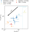 |
Fig. 8 Variation of flux ratios, FCO2/FC2H2 and F13CO2/F13CCH2, across different SFRs or moving groups. We include Sz114 (Xie et al. 2023). The dashed line indicates a line with slope of unity. Due to the non-detections of both 13CO2 and 13CCH2 in J0438, we present it with a vertical dotted line. The colors indicate the different SFRs or the moving groups shown in the legend at the top. The ages indicated are canonical values commonly used in the literature; however, recent studies indicate a larger diversity in the ages of sources within each SFR (e.g., Ratzenböck et al. 2023). |
5.2 Signatures of disk evolution in inner and outer disk dust
While transport processes are suggested to enhance the C/O in the inner disk (Mah et al. 2023), efficient grain growth and dust settling as predicted by Pinilla et al. (2013) would lead to a decrease in the number density of small dust in the surface layers that largely carry the continuum opacity in the infrared wavelengths. Thus, grain growth and settling would lead to weaker dust features and allow us to probe deeper layers of the disk in the infrared (in other words, large columns of gas). In fact, this is what we find in Sect. 4.2, i.e., disks with larger gas columns (F13CCH2/FC2H2) show weaker dust strengths (F9.8).
Further, rapid inward transport of material would deplete the outer disk pebbles, leading to smaller disk masses (Liu et al. 2020) and lower continuum fluxes at millimeter wavelengths for evolved disks. In Sect. 4.3, we do find a trend that disks with higher C2H2 gas columns have lower disk dust masses.
The observed trends in millimeter and infrared dust signatures are in line with models that predict high C/O by transport processes (Mah et al. 2023). However, this does not completely rule out the possibility of C/O enhancement by carbon grain destruction or dust traps locking up H2O ice. Moreover, the above comparisons are qualitative, and a more quantitative comparison between such models and observed data is required.
5.3 Spectral appearance and the disk structure
In Sect. 4.2, we show that sources with higher gas columns (F13CCH2/FC2H2) exhibit weaker CO2 and H2O fluxes relative to C2H2. Although VLMS disks generally show less diverse oxygen-bearing molecules than T Tauri disks (Sect. 4.4), the VLMS disks more commonly show the presence of 13CO2, possibly indicating a larger observable column of CO2 than typical T Tauri disks. As shown by Arabhavi et al. (2025), lower detection rates of oxygen-bearing molecules in the carbon-rich VLMS disks can simply be due to the emission from C2H2 and other hydrocarbons outshining the emission from the oxygen-bearing molecules. In general, the spectral appearance of the disk is strongly influenced by two important factors: the spatial distribution of different chemical species and the continuum optical depth surface (τdust=1). These are in turn related to the grain growth and C/O enhancement timescales, and the inner disk substructure.
5.3.1 Role of dust opacity
Figure 9 shows a possible evolution pathway for the τdust=1 surface that could explain the observed trends in Sect. 4.2. Woitke et al. (2018b) showed that the emission from different molecules arises from onion-like layers at different depths (at solar C/O). In such a scenario, changes in dust opacities can expose different chemical layers. We neglect the feedback that the change in opacities can have on chemistry, which can be important. As the disk evolves, the lower dust opacity due to grain growth shifts the τdust=1 layer deeper in the disk. Following the structure in Woitke et al. (2018b), H2O is at the top, followed by CO2, and even deeper is the C2H2 emitting layer. In addition, Kanwar et al. (2024a) show that C2H2, and in general the hydrocarbons, have two reservoirs, one in the surface layer and the other much closer to the midplane.
When the τdust=1 layer is high up in the disk, only the gas in the warm surface layers emits. The spectra would appear oxygen-rich (dominated by water) similar to T Tauri disks as a result of weak emission from C2H2 and other hydrocarbons due to their low column densities above the τdust=1 layer. Any C2H2 emission would be weak but warm; a good example of this would be the MIRI spectrum of Sz114 (Xie et al. 2023).
A slightly lower τ=1 layer would lead to much brighter but optically thin (i.e., no molecular continuum) C2H2 emission. The brightness of C2H2, CO2, and H2O would be related to the radial extent of these species. Gaps and cavities can have a strong influence on the flux levels. Depending on the radial extent and abundance of C2H2 and H2O in the surface layers, the spectral appearance could vary from C2H2-bright (e.g., J1558) to H2O-bright (e.g., J0438).
An even deeper τ=1 layer would allow gas emission from layers increasingly closer to the midplane. In such cases, while H2O and CO2 would still emit from the surface layers, a deeper reservoir of hydrocarbons would now emit much stronger than H2O. Arabhavi et al. (2025) show that there is a strong change in the peak-to-continuum ratio of C2H2 in the sample, and a weak change of CO2, but not for water. CO2 would still be visible due to the prominent Q–branch (see Fig. 6 of Arabhavi et al. 2025) and 13CO2 would be visible due to the large column density of CO2 above the τ=1 layer. Deeper gas columns would reflect lower C2H2 temperatures compared to when the τ=1 surface is higher up in the disk. The trend observed in the diversity of oxygen-carriers (Fig. 7) could simply be due to the strong hydrocarbon emission in disks of lower stellar luminosities outshining the oxygen-bearing species.
Although we neglected the effects of changing dust opacity on the temperature and chemistry of the gas, a lower dust opacity could allow more energy to be absorbed by the gas compared to cases with higher opacity. This may result in elevated gas temperatures (e.g., see Greenwood et al. 2019). Deeper penetration of UV radiation can strongly influence the chemical composition of the disk (e.g., see Greenwood et al. 2019), but large columns of molecules can shield themselves and other molecules (e.g., Bosman et al. 2022; Woitke et al. 2024). To accurately assess the influence of the change in dust opacity on gas temperature and chemistry, and the validity of the scenarios presented in Fig. 9, detailed modeling that includes molecular self-shielding – especially among the many hydrocarbons – is essential. Another important factor affecting the temperatures is the luminosity of the central objects, which generally decreases with age (e.g., Nelson et al. 1986); moreover, stellar activity can also have a strong impact on the thermal structure and chemical evolution of the disk.
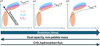 |
Fig. 9 Cartoon illustrating the role of dust opacity on the mid-IR spectral appearance. The dotted line represents the τdust=1 layer. Cyan, pink, and orange ellipses represent the H2O, CO2, and the two C2H2 reservoirs. The arrows show the direction of increase in the quantity mentioned. |
5.3.2 Role of C/O
The strong spectral signatures of hydrocarbons and weaker dust opacity would still require a hydrocarbon reservoir with a C/O greater than unity (Kanwar et al. 2024a, Woitke et al. 2018b). However, Kanwar et al. (2024a) show that even in an enhanced C/O environment (as high as C/O=2), large column densities (>1018 cm−2) of H2O and CO2 can still be present. This is in line with the analysis of water in our sample (Arabhavi et al. 2025).
Woitke et al. (2018a) show that condensation of elements, starting from solar abundances, could enhance the gas phase C/O, but only up to about 0.83 at temperatures of ~300 K. This suggests that more extreme processes are required to increase the gas phase C/O to beyond unity.
Such enhancements are more likely in a VLMS disk than in a T Tauri disk (Mah et al. 2023). For example, rapid transport processes could enhance the C/O in the inner disk, while grain growth would allow us to probe much deeper into the disk. These two processes together could render the spectral appearance of an evolved disk appear very carbon-rich. Although dust growth and inward transport can also occur in a T-Tauri disk, they are less efficient than in VLMS disks (Pinilla et al. 2013; Mah et al. 2023).
Rapid inward transport of material in VLMS disks would lead to an oxygen-depleted disk with a high C/O. However, C/O enhancement can also occur through gas-phase carbon enrichment by the destruction of carbon in dust grains (Tabone et al. 2023) or trapping oxygen-rich ices in the outer disk (Mah et al. 2024). Arabhavi et al. (2024) point out that oxygen depletion and carbon enrichment scenarios could lead to measurable differences in the gas and dust compositions of the disk. While the observed trends in the infrared and millimeter wavelengths favor the rapid transport scenario, carbon enrichment by carbon grain destruction can occur simultaneously or even be the main C/O enriching process in the midplane closer to the star.
The efficiency of transport processes varies with height above the disk midplane, potentially leading to vertical stratification in the C/O. Additionally, steep vertical gradients in gas temperatures and UV radiation in the disk can contribute to stratified carbon grain destruction. Whether such stratification persists over the disk evolution timescales depends on the strength of vertical mixing. Efficient vertical mixing acts to remove this vertical stratification of elemental abundances (Woitke et al. 2022). This mixing can also change the molecular abundances in the layers probed in the mid-infrared (Heinzeller et al. 2011; Woitke et al. 2022). For example, Woitke et al. (2022) found that stronger vertical mixing leads to richer hydrocarbon chemistry in the upper layers, leading to an increase in C2H2 fluxes of more than an order of magnitude. Importantly, this enhanced hydrocarbon emission does not necessarily indicate a carbon-rich environment, as water abundances are also elevated. As shown by Arabhavi et al. (2025), once the hydrocarbon column densities exceed a critical threshold, they can outshine water emission – even when column densities of water are higher overall.
Further analyses by retrieving the column densities, temperatures, and emitting area of the gas emission, as well as the chemical composition of the dust grains, or by full forward modeling (e.g., Woitke et al. 2024) of the entire MIRI spectrum can provide strong constraints on the C/O enhancement processes. Kanwar et al. (2024b) show that using multiple (>2) molecular emissions, it might be possible to distinguish between the C/O enhancement processes.
Robust spatially resolved ALMA observations would provide valuable insight into the importance of disk substructures that can trap oxygen-rich material in the outer disk. It is important to note here that all of our sources were selected based on the rationale that they were previously studied with Spitzer. This could introduce a bias toward brighter VLMS targets. A larger sample of VLMS sources would further test our findings and expand our understanding of disk evolution.
Finally, since some of the C/O enrichment processes could occur in T Tauri disks, possibly at a different rate, a comparison study between VLMS and T Tauri disk spectra can provide valuable insights into the inner disk environments (e.g., Grant et al., in preparation.). Parameter exploration using thermochemical models to understand the role of inner disk substructures and elemental composition in the mid-infrared spectra of the VLMS disks would be insightful in conjunction with these observations. Expanding dynamic models such as Mah et al. (2023) to 2D and deriving molecular mid-infrared spectra would provide a better understanding of the interplay between dust evolution and chemical composition.
6 Conclusions
We present the MIRI spectra of disks around ten VLMS with central objects ranging from 0.02 M⊙ to 0.14 M⊙, across three SFRs and one moving group. We draw the following conclusions based on the analysis of these spectra:
The VLMS spectra show a diversity of dust features. In agreement with the Spitzer results, these dust features are typically broader and weaker than in the disks around higher-mass stars.
The spectra are rich in molecular emission. We detect H I, [Ar II], [Ne II], H2, OH, H2O, CO, CO2, HCN, HC3N, CH3, CH4, C2H2, C2H4, C2H6, C3H4, C4H2, C6H6, 13CO2, and 13CCH2 in the sample.
Organic molecules dominate the molecular emission. The most commonly detected molecules are C2H2 and HCN, followed by CO2, C4H2, and C6H6.
The detection rates of organic molecules correlate with other organic molecules while anticorrelating with inorganic molecules.
Spectra with a higher F13CCH2/FC2H2 ratio (a proxy for column density of gas probed by MIRI) show detections of a large number of hydrocarbons. The ratio also anticorrelates with the 10 μm dust strengths, disk dust mass, stellar luminosity, and the flux ratios of oxygen-bearing molecules to acetylene (FH2O/FC2H2 and FCO2/FC2H2).
We find tentative evidence for the chemical evolution from young oxygen-rich disks to older carbon-rich disks. The anticorrelations with the 10 μm dust strength and the disk dust mass suggest rapid inward material transport and grain growth in-line with model predictions such as Mah et al. (2023).
In this paper, we analyzed the gas emission in the MINDS VLMS sample. We refer to Jang et al. (in prep.) for a detailed analysis of the dust in these disks and Arabhavi et al. (2025) for an overview of oxygen-bearing molecules in these disks.
Acknowledgements
This work is based on observations made with the NASA/ESA/CSA James Webb Space Telescope. The data were obtained from the Mikulski Archive for Space Telescopes at the Space Telescope Science Institute, which is operated by the Association of Universities for Research in Astronomy, Inc., under NASA contract NAS 5-03127 for JWST. These observations are associated with program #1282. The following National and International Funding Agencies funded and supported the MIRI development: NASA; ESA; Belgian Science Policy Office (BELSPO); Centre Nationale d’Etudes Spatiales (CNES); Danish National Space Centre; Deutsches Zentrum fur Luft- und Raumfahrt (DLR); Enterprise Ireland; Ministerio De Economía y Competividad; Netherlands Research School for Astronomy (NOVA); Netherlands Organisation for Scientific Research (NWO); Science and Technology Facilities Council; Swiss Space Office; Swedish National Space Agency; and UK Space Agency. I.K., A.M.A., and E.v.D. acknowledge support from grant TOP-1 614.001.751 from the Dutch Research Council (NWO). A.C.G. acknowledges support from PRINMUR 2022 20228JPA3A “The path to star and planet formation in the JWST era (PATH)” funded by NextGeneration EU and by INAF-GoG 2022 “NIR-dark Accretion Outbursts in Massive Young stellar objects (NAOMY)” and Large Grant INAF 2022 “YSOs Outflows, Disks and Accretion: towards a global framework for the evolution of planet forming systems (YODA)”. G.P. gratefully acknowledges support from the Max Planck Society and from the Carlsberg Foundation, grant CF23-0481. E.v.D. acknowledges support from the ERC grant 101019751 MOLDISK and the Danish National Research Foundation through the Center of Excellence “InterCat” (DNRF150). T.H. and K.S. acknowledge support from the European Research Council under the Horizon 2020 Framework Program via the ERC Advanced Grant Origins 8324 28. I.K. and J.K. acknowledge funding from H2020-MSCA-ITN-2019, grant no. 860470 (CHAMELEON). B.T. is a Laureate of the Paris Region fellowship program, which is supported by the Ile-de-France Region and has received funding under the Horizon 2020 innovation framework program and Marie Sklodowska-Curie grant agreement No. 945298. V.C. acknowledge funding from the Belgian F.R.S.-FNRS. D.G. thanks the Belgian Federal Science Policy Office (BELSPO) for the provision of financial support in the framework of the PRODEX Programme of the European Space Agency (ESA). D.B. and M.M.C. have been funded by Spanish MCIN/AEI/10.13039/501100011033 grants PID2019-107061GB-C61 and No. MDM-2017-0737. M.T., M.V. and A.D.S acknowledge support from the ERC grant 101019751 MOLDISK. I.P. acknowledges partial support by NASA under agreement No. 80NSSC21K0593 for the program “Alien Earths”. P.P. thanks the Swiss National Science Foundation (SNSF) for financial support under grant number 200020_200399.
Appendix A De-reddening and continuum definition
Figure A.1 shows the MIRI spectra before and after de-reddening. The extinction values and the references are listed in Table 1. The literature values of the extinctions are based on the extinction curve given by Cardelli et al. (1989) assuming Rv=3.1. However, this does not extend to the entire MIRI wavelength range. Hence, we use the extinction curve described in Gordon et al. (2023). The spectra are normalized to 150 pc.
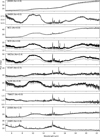 |
Fig. A.1 Spectra before (gray) and after (black) de-reddening. |
Figure A.2 shows the continuum curves used in this paper. As explained in Sect. 2.3, we use a narrow and a broad Savitzky-Golay filter to determine two sets of continua for our sample (shown in red and blue in the figure, respectively). The broad width continuum (blue) is only used to measure the dust strength and the line fluxes of C2H2, and hence the shape of this continuum beyond 14 μm or shortward of 8 μm is not important. The narrow width continuum (red) is used to measure the line fluxes of all the other molecules used in the analysis of the paper. The spectra are normalized to 150 pc.
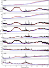 |
Fig. A.2 Continuum definition. The observed MIRI spectra are shown in black; the continua with narrow Savitzky-Golay filter are shown in red and the continua with broad Savitzky-Golay filter are shown in blue. |
Appendix B Comparison with Spitzer
Figure B.1 compares the MIRI observations with the Spitzer spectra (both normalized to 150 pc). The Spitzer specrta were taken from Pascucci et al. (2009), Pascucci et al. (2013), and CASSIS (Lebouteiller et al. 2011, Lebouteiller et al. 2015). In general the MIRI spectra seem to match well with the Spitzer spectra. In some sources there seem to be some flux differences. For example, J0438 shows a seesaw variability (more details in Perotti et al. 2025). In some sources (e.g., Sz28, HKCha, and J1558), there is a flux discrepancy between MIRI and Spitzer. This is more evident at the 10 μm dust feature.
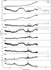 |
Fig. B.1 Comparison of the MIRI observations with Spitzer spectra. |
Appendix C Detection criteria
The VLMS spectra are typically show rich molecular emission as can be seen in Fig. 1. In all of our sources, the S/N is above 100 in the spectral windows where molecular emissions are observed (more details on the S/N calculation from the ETC is presented in Jang et al. in prep.). Most of the molecular emission overlap in their wavelengths, and their detectability is influenced more by the surrounding molecular emission rather than the noise. i.e., defining a simple criteria classifying a Q-branch peak of a species above 3 σ as a detection, similar to the case of T Tauri disks, is not complete. The detection criteria should also account for neighboring molecular emission. This requires fitting the spectra with slab models, which is beyond the scope of this work. Instead we include all the detections reported by the previous publications on individual sources:
J0438: Perotti et al. (2025)
NC1: Morales-Calderón et al. (2025)
IC147: Arabhavi et al. (2024)
TWA27: Patapis et al. in preparation
For the remaining sources (NC9, J0439, HKCha, and J1558) we refer to Arabhavi et al. (2025) for discussion on detections of H2O, OH, and CO. The rest of the atomic and molecular detections are illustrated in Figs. C.1–C.4. The synthetic molecular spectra in these figures and generated from slab models introduced in Arabhavi et al. (2024). In the J1558 spectrum (bottom left panel of Fig. C.3), the CO2 model Q-branch peak matches with one of the observed peaks but the shape does not – the broader shoulder on the short wavelength side of the peak is missing in the observed spectrum. There is also a pure rotational water line (199,10−188,11) with high Einstein A coefficient that matches the peak. Proper modeling of the source is required to confirm the presence of CO2. In the panels on the right, while some peaks match with the observed spectrum of HKCha and J0439, some at ~16.6 μm do not. This can be due to several factors such as different continuum levels, excitation conditions, or simply the absence of CH3. Again, proper modeling of the spectra is required for these sources. The top and middle panels of Fig. C.4 shows hints of CH4 and C2H4, and the bottom panel shows firm detection of C2H6. In addition to previous detections in J1605, we detect CH3 (Fig. C.5).
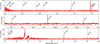 |
Fig. C.1 Detections of atomic and molecular hydrogen lines in the J1558 spectrum. The continuum-subtracted MIRI spectrum is shown in red. The atomic and molecular hydrogen lines are marked by vertical dashed lines and are labeled. The two lines with question marks indicate line emissions that could be possibly blended with CO ro-vibration lines. |
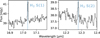 |
Fig. C.2 Detections of molecular hydrogen line emission in the HKCha spectrum. The MIRI spectrum is shown in black. |
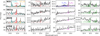 |
Fig. C.3 Detections of molecular emission in NC9, HKCha, J0439, and J1558. The MIRI spectra are shown in black. The different molecular emissions are shown using slab model spectra as color-filled regions in each panel. The question mark (?) indicates that additional modeling is needed to confirm the detection. |
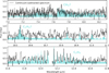 |
Fig. C.4 Detections of molecular emission in NC9. The continuum-subtracted MIRI spectrum is shown in black. The different molecular emissions are shown using slab model spectra as color-filled regions in each panel. The question mark (?) indicates that additional modeling is needed to confirm the detection. |
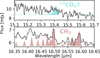 |
Fig. C.5 Detections of molecular emission in J1605. The MIRI spectrum is shown in black. The different molecular emissions are shown using slab model spectra as color-filled regions in each panel. The question mark (?) indicates that additional modeling is needed to confirm the detection. |
Appendix D Detection rate correlations
Figure D.1 shows the binary correlation coefficients for the molecules detected in the spectra. Since the species detected in all sources and those detected in only one source do not provide useful correlations, those species are not shown. The correlations and anticorrelations are indicated by colors varying from blue to red. Interestingly, Fig. D.1 shows three distinct regions: (i) the blue-dominated region to the left of the figure, which largely indicates correlations between organic molecule pairs; (ii) the smaller blue region at the bottom, which shows correlations between the inorganic species; and (iii) the red region on the right that shows the anticorrelation between the organic molecules and inorganic species. We also calculate the p-value using the Fisher’s exact test (scipy.stats.fisher_exact). We find statistically significant strong correlations between less abundant hydrocarbons, and statistically significant strong anticorrelations between less abundant hydrocarbons and inorganic molecules.
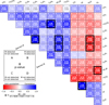 |
Fig. D.1 Binary correlation coefficients (Yule 1912) between the detection rates of different molecules. The box on the bottom left describes the details of various numbers shown in each colored box on the right. The color denotes the value of the correlation coefficient, with red corresponding to an anticorrelation and blue corresponding to a correlation. For calculating the coefficients only firm detections are considered as “detected” while the rest (including tentative detections) are considered “undetected.” Molecules that are detected in all the sources or are detected in only one source are not shown. Molecule pairs with statistically significant correlations (p-value <0.05) are highlighted with black borders. |
References
- Andrews, S. M., Rosenfeld, K. A., Kraus, A. L., & Wilner, D. J. 2013, ApJ, 771, 129 [Google Scholar]
- Antonellini, S., Kamp, I., Riviere-Marichalar, P., et al. 2015, A&A, 582, A105 [NASA ADS] [CrossRef] [EDP Sciences] [Google Scholar]
- Apai, D., Pascucci, I., Bouwman, J., et al. 2005, Science, 310, 834 [NASA ADS] [CrossRef] [Google Scholar]
- Arabhavi, A. M., Kamp, I., Henning, T., et al. 2024, Science, 384, 1086 [NASA ADS] [CrossRef] [Google Scholar]
- Arabhavi, A. M., Kamp, I., van Dishoeck, E. F., et al. 2025, ApJ, 984, L62 [Google Scholar]
- Argyriou, I., Glasse, A., Law, D. R., et al. 2023, A&A, 675, A111 [NASA ADS] [CrossRef] [EDP Sciences] [Google Scholar]
- Barenfeld, S. A., Carpenter, J. M., Ricci, L., & Isella, A. 2016, ApJ, 827, 142 [Google Scholar]
- Basri, G., Mohanty, S., Allard, F., et al. 2000, ApJ, 538, 363 [NASA ADS] [CrossRef] [Google Scholar]
- Bosman, A. D., Bergin, E. A., Calahan, J., & Duval, S. E. 2022, ApJ, 930, L26 [NASA ADS] [CrossRef] [Google Scholar]
- Burn, R., Schlecker, M., Mordasini, C., et al. 2021, A&A, 656, A72 [NASA ADS] [CrossRef] [EDP Sciences] [Google Scholar]
- Bushouse, H., Eisenhamer, J., Dencheva, N., et al. 2023, https://doi.org/10.5281/zenodo.7692609 [Google Scholar]
- Cardelli, J. A., Clayton, G. C., & Mathis, J. S. 1989, ApJ, 345, 245 [Google Scholar]
- Christiaens, V., Gonzalez, C., Farkas, R., et al. 2023, J. Open Source Softw., 8, 4774 [NASA ADS] [CrossRef] [Google Scholar]
- Christiaens, V., Samland, M., Gasman, D., Temmink, M., & Perotti, G. 2024, Astrophysics Source Code Library [record ascl:2403.007] [Google Scholar]
- Colmenares, M. J., Bergin, E. A., Salyk, C., et al. 2024, ApJ, 977, 173 [NASA ADS] [CrossRef] [Google Scholar]
- Decleir, M., Gordon, K. D., Andrews, J. E., et al. 2022, ApJ, 930, 15 [NASA ADS] [CrossRef] [Google Scholar]
- Erb, D. 2022, https://doi.org/10.5281/zenodo.7255880 [Google Scholar]
- Fedele, D., van den Ancker, M. E., Henning, T., Jayawardhana, R., & Oliveira, J. M. 2010, A&A, 510, A72 [NASA ADS] [CrossRef] [EDP Sciences] [Google Scholar]
- Fitzpatrick, E. L., Massa, D., Gordon, K. D., Bohlin, R., & Clayton, G. C. 2019, ApJ, 886, 108 [Google Scholar]
- Flagg, L., Scholz, A., Almendros-Abad, V., et al. 2025, arXiv e-prints [arXiv:2505.13714] [Google Scholar]
- Gaia Collaboration (Brown, A. G. A., et al.) 2021, A&A, 649, A1 [NASA ADS] [CrossRef] [EDP Sciences] [Google Scholar]
- Gasman, D., van Dishoeck, E. F., Grant, S. L., et al. 2023, A&A, 679, A117 [NASA ADS] [CrossRef] [EDP Sciences] [Google Scholar]
- Gomez Gonzalez, C. A., Wertz, O., Absil, O., et al. 2017, AJ, 154, 7 [Google Scholar]
- Gordon, K. D., Cartledge, S., & Clayton, G. C. 2009, ApJ, 705, 1320 [NASA ADS] [CrossRef] [Google Scholar]
- Gordon, K. D., Misselt, K. A., Bouwman, J., et al. 2021, ApJ, 916, 33 [NASA ADS] [CrossRef] [Google Scholar]
- Gordon, K. D., Clayton, G. C., Decleir, M., et al. 2023, ApJ, 950, 86 [CrossRef] [Google Scholar]
- Gordon, K. D., 2024, J. Open Source Software, 9, 7023 [Google Scholar]
- Grant, S. L., van Dishoeck, E. F., Tabone, B., et al. 2023, ApJ, 947, L6 [NASA ADS] [CrossRef] [Google Scholar]
- Greenwood, A. J., Kamp, I., Waters, L. B. F. M., et al. 2017, A&A, 601, A44 [NASA ADS] [CrossRef] [EDP Sciences] [Google Scholar]
- Greenwood, A. J., Kamp, I., Waters, L. B. F. M., Woitke, P., & Thi, W. F. 2019, A&A, 631, A81 [NASA ADS] [CrossRef] [EDP Sciences] [Google Scholar]
- Güdel, M., Briggs, K. R., Arzner, K., et al. 2007, A&A, 468, 353 [Google Scholar]
- Heinzeller, D., Nomura, H., Walsh, C., & Millar, T. J. 2011, ApJ, 731, 115 [NASA ADS] [CrossRef] [Google Scholar]
- Henning, T. K., & Krasnokutski, S. A. 2019, Nat. Astron., 3, 568 [Google Scholar]
- Herczeg, G. J., & Hillenbrand, L. A. 2008, ApJ, 681, 594 [Google Scholar]
- Herczeg, G. J., & Hillenbrand, L. A. 2014, ApJ, 786, 97 [Google Scholar]
- Henning, T., Kamp, I., Samland, M., et al. 2024, PASP, 136, 054302 [NASA ADS] [CrossRef] [Google Scholar]
- Kaeufer, T., Min, M., Woitke, P., Kamp, I., & Arabhavi, A. M. 2024a, A&A, 687, A209 [NASA ADS] [CrossRef] [EDP Sciences] [Google Scholar]
- Kaeufer, T., Woitke, P., Kamp, I., Kanwar, J., & Min, M. 2024b, A&A, 690, A100 [NASA ADS] [CrossRef] [EDP Sciences] [Google Scholar]
- Kalyaan, A., Pinilla, P., Krijt, S., et al. 2023, ApJ, 954, 66 [NASA ADS] [CrossRef] [Google Scholar]
- Kamp, I., Thi, W. F., Woitke, P., et al. 2017, A&A, 607, A41 [NASA ADS] [CrossRef] [EDP Sciences] [Google Scholar]
- Kamp, I., Henning, T., Arabhavi, A. M., et al. 2023, Faraday Discuss., 245, 112 [NASA ADS] [CrossRef] [Google Scholar]
- Kanwar, J., Kamp, I., Jang, H., et al. 2024a, A&A, 689, A231 [NASA ADS] [CrossRef] [EDP Sciences] [Google Scholar]
- Kanwar, J., Kamp, I., Woitke, P., et al. 2024b, A&A, submitted [Google Scholar]
- Kessler-Silacci, J. E., Dullemond, C. P., Augereau, J. C., et al. 2007, ApJ, 659, 680 [NASA ADS] [CrossRef] [Google Scholar]
- Lebouteiller, V., Barry, D. J., Spoon, H. W. W., et al. 2011, ApJS, 196, 8 [NASA ADS] [CrossRef] [Google Scholar]
- Lebouteiller, V., Barry, D. J., Goes, C., et al. 2015, ApJS, 218, 21 [Google Scholar]
- Lienert, J. L., Bitsch, B., & Henning, T. 2024, A&A, 691, A72 [NASA ADS] [CrossRef] [EDP Sciences] [Google Scholar]
- Liu, Y., Pascucci, I., & Henning, T. 2019, A&A, 623, A106 [NASA ADS] [CrossRef] [EDP Sciences] [Google Scholar]
- Liu, B., Lambrechts, M., Johansen, A., Pascucci, I., & Henning, T. 2020, A&A, 638, A88 [EDP Sciences] [Google Scholar]
- Long, F., Pascucci, I., Houge, A., et al. 2025, ApJ, 978, L30 [Google Scholar]
- Luhman, K. L. 2007, ApJS, 173, 104 [Google Scholar]
- Luhman, K. L. 2012, ARA&A, 50, 65 [CrossRef] [Google Scholar]
- Luhman, K. L., Adame, L., D’Alessio, P., et al. 2007, ApJ, 666, 1219 [Google Scholar]
- Mah, J., Bitsch, B., Pascucci, I., & Henning, T. 2023, A&A, 677, L7 [CrossRef] [EDP Sciences] [Google Scholar]
- Mah, J., Savvidou, S., & Bitsch, B. 2024, A&A, 686, L17 [NASA ADS] [CrossRef] [EDP Sciences] [Google Scholar]
- Manara, C. F., Robberto, M., Da Rio, N., et al. 2012, ApJ, 755, 154 [NASA ADS] [CrossRef] [Google Scholar]
- Manara, C. F., Fedele, D., Herczeg, G. J., & Teixeira, P. S. 2016, A&A, 585, A136 [NASA ADS] [CrossRef] [EDP Sciences] [Google Scholar]
- Manara, C. F., Testi, L., Herczeg, G. J., et al. 2017, A&A, 604, A127 [NASA ADS] [CrossRef] [EDP Sciences] [Google Scholar]
- Manara, C. F., Ansdell, M., Rosotti, G. P., et al. 2023, ASP Conf. Ser., 534, 539 [NASA ADS] [Google Scholar]
- Manjavacas, E., Tremblin, P., Birkmann, S., et al. 2024, AJ, 167, 168 [NASA ADS] [CrossRef] [Google Scholar]
- Morales-Calderón, M., Jang, H., Arabhavi, A. M., et al. 2025, A&A, submitted [Google Scholar]
- Muzerolle, J., Luhman, K. L., Briceño, C., Hartmann, L., & Calvet, N. 2005, ApJ, 625, 906 [NASA ADS] [CrossRef] [Google Scholar]
- Nelson, L. A., Rappaport, S. A., & Joss, P. C. 1986, ApJ, 311, 226 [Google Scholar]
- Pascucci, I., Apai, D., Luhman, K., et al. 2009, ApJ, 696, 143 [Google Scholar]
- Pascucci, I., Herczeg, G., Carr, J. S., & Bruderer, S. 2013, ApJ, 779, 178 [NASA ADS] [CrossRef] [Google Scholar]
- Pascucci, I., Testi, L., Herczeg, G. J., et al. 2016, ApJ, 831, 125 [Google Scholar]
- Perotti, G., Kurtovic, N. T., Henning, T., et al. 2025, arXiv e-prints [arXiv:2504.11424] [Google Scholar]
- Pinilla, P., Birnstiel, T., Benisty, M., et al. 2013, A&A, 554, A95 [NASA ADS] [CrossRef] [EDP Sciences] [Google Scholar]
- Ratzenböck, S., Großschedl, J. E., Alves, J., et al. 2023, A&A, 678, A71 [NASA ADS] [CrossRef] [EDP Sciences] [Google Scholar]
- Rebull, L. M., Padgett, D. L., McCabe, C. E., et al. 2010, ApJS, 186, 259 [NASA ADS] [CrossRef] [Google Scholar]
- Riaz, B., & Gizis, J. E. 2008, ApJ, 681, 1584 [CrossRef] [Google Scholar]
- Ricci, L., Cazzoletti, P., Czekala, I., et al. 2017, AJ, 154, 24 [NASA ADS] [CrossRef] [Google Scholar]
- Rice, E. L., Barman, T., Mclean, I. S., Prato, L., & Kirkpatrick, J. D. 2010, ApJS, 186, 63 [NASA ADS] [CrossRef] [Google Scholar]
- Rieke, G. H., Wright, G., Böker, T., et al. 2015, Publ. Astron. Soc. Pac., 127, 584 [Google Scholar]
- Sabotta, S., Schlecker, M., Chaturvedi, P., et al. 2021, A&A, 653, A114 [NASA ADS] [CrossRef] [EDP Sciences] [Google Scholar]
- Scholz, A., Jayawardhana, R., & Wood, K. 2006, ApJ, 645, 1498 [NASA ADS] [CrossRef] [Google Scholar]
- Schwarz, K. R., Henning, T., Christiaens, V., et al. 2024, ApJ, 962, 8 [NASA ADS] [CrossRef] [Google Scholar]
- Sellek, A. D., Vlasblom, M., & van Dishoeck, E. F. 2025, A&A, 694, A79 [NASA ADS] [CrossRef] [EDP Sciences] [Google Scholar]
- Tabone, B., Bettoni, G., van Dishoeck, E. F., et al. 2023, Nat. Astron., 7, 805 [NASA ADS] [CrossRef] [Google Scholar]
- Temmink, M., van Dishoeck, E. F., Grant, S. L., et al. 2024, A&A, 686, A117 [NASA ADS] [CrossRef] [EDP Sciences] [Google Scholar]
- Testi, L., Natta, A., Manara, C. F., et al. 2022, A&A, 663, A98 [NASA ADS] [CrossRef] [EDP Sciences] [Google Scholar]
- van der Marel, N., & Pinilla, P. 2023, arXiv e-prints [arXiv:2310.09077] [Google Scholar]
- Vlasblom, M., Temmink, M., Grant, S. L., et al. 2025, A&A, 693, A278 [NASA ADS] [CrossRef] [EDP Sciences] [Google Scholar]
- Ward-Duong, K., Patience, J., Bulger, J., et al. 2018, AJ, 155, 54 [NASA ADS] [CrossRef] [Google Scholar]
- Wells, M., Pel, J. W., Glasse, A., et al. 2015, PASP, 127, 646 [NASA ADS] [CrossRef] [Google Scholar]
- White, R. J., & Basri, G. 2003, ApJ, 582, 1109 [Google Scholar]
- Woitke, P., Helling, C., Hunter, G. H., et al. 2018a, A&A, 614, A1 [NASA ADS] [CrossRef] [EDP Sciences] [Google Scholar]
- Woitke, P., Min, M., Thi, W. F., et al. 2018b, A&A, 618, A57 [NASA ADS] [CrossRef] [EDP Sciences] [Google Scholar]
- Woitke, P., Arabhavi, A. M., Kamp, I., & Thi, W. F. 2022, A&A, 668, A164 [NASA ADS] [CrossRef] [EDP Sciences] [Google Scholar]
- Woitke, P., Thi, W. F., Arabhavi, A. M., et al. 2024, A&A, 683, A219 [NASA ADS] [CrossRef] [EDP Sciences] [Google Scholar]
- Woods, P. M., & Willacy, K. 2007, ApJ, 655, L49 [NASA ADS] [CrossRef] [Google Scholar]
- Woods, P. M., & Willacy, K. 2009, ApJ, 693, 1360 [Google Scholar]
- Wright, G. S., Wright, D., Goodson, G. B., et al. 2015, PASP, 127, 595 [NASA ADS] [CrossRef] [Google Scholar]
- Wright, G. S., Rieke, G. H., Glasse, A., et al. 2023, PASP, 135, 048003 [NASA ADS] [CrossRef] [Google Scholar]
- Xie, C., Pascucci, I., Long, F., et al. 2023, ApJ, 959, L25 [NASA ADS] [CrossRef] [Google Scholar]
- Yule, G. U. 1912, J. R. Stat. Soc., 75, 579 [CrossRef] [Google Scholar]
Tests carried out after completing the analysis presented in this work revealed that as of v1.14 onward, the bad pixel correction performed using default parameters of the official pipeline now leads to similar quality spectra as obtained with the VIP-based bad pixel correction.
A single point model with a column density, temperature, and an emitting radius.
All Tables
All Figures
|
Fig. 1 Summary of dust and gas observations. The left panels show continuum-normalized dust strengths highlighting SiO2, enstatite, and forsterite emission features. The middle panels present a close-up of the observed C2H2 features, highlighting four peaks corresponding to the main and rare isotopologues in red and blue, respectively. The right panels show the continuum-subtracted hydrocarbon-rich wavelength region of the spectra. The gray regions highlight the main Q branches of molecules in this wavelength region. HCN* and |
| In the text | |
|
Fig. 2 Summary of dust and gas detections in the sample. The green square refers to a firm detection, the yellow square indicates a tentative detection, and the light gray square indicates a non-detection. The top panel shows the number of detections for each species. The right panel shows the number of species of two groups detected in each source. The inorganic species (dark gray) include H2, H2O, HI, CO, CO2, 13CO2, [Ne II], and OH. The organic species (faded red) include all the hydrocarbons and cyanomolecules. The hatched region in the top and right panels shows tentative detections. |
| In the text | |
|
Fig. 3 Comparison of the 10 μm dust feature of NC1 (VLMS) and SY Cha (T Tauri). Here the continuum-normalized flux is shown. The observed MIRI spectrum of SY Cha is taken from Schwarz et al. (2024). |
| In the text | |
|
Fig. 4 Binary correlation coefficients between the detection rates of a few species with strong (anti)correlations. Correlation coefficients (and the p-values) for a more extended list of species are shown in Fig. D.1. |
| In the text | |
|
Fig. 5 Trends in the MIRI observations. Panels A-D show the number of hydrocarbons (CnHm) detected, the integrated dust strength, the CO2 to C2H2 flux ratios, and the H2O to C2H2 flux ratios against the flux ratio F13CCH2/FC2H2, along with the error bars. The molecules with tentative or non-detections are indicated by the upper limits. In case of non-detections, we report the 1σ upper limits. All error bars are 1σ with an assumption of a S/N of 100. |
| In the text | |
|
Fig. 6 Trends in stellar and disk properties. Panels A-C show the dust mass (estimated from 0.89 mm continuum fluxes), stellar luminosity, and mass accretion rate against the flux ratio F13CCH2/FC2H2. |
| In the text | |
|
Fig. 7 Luminosities of the central object against oxygen-bearing molecules in the inner disks. The colored boxes refer to the oxygen-bearing molecules detected in the MIRI spectra of each source, indicated in the legend. Tentative detections are highlighted by white crosses. The VLMS disks are highlighted in bold. The detection in T Tauri disks are taken from the following papers: GW Lup (Grant et al. 2023), Sz 98 (Gasman et al. 2023), DR Tau (Temmink et al. 2024), SY Cha (Schwarz et al. 2024), CX Tau (Vlasblom et al. 2025), and V1094Sco (Tabone et al. in prep.). Detections of Sz114 are obtained from Xie et al. (2023). |
| In the text | |
|
Fig. 8 Variation of flux ratios, FCO2/FC2H2 and F13CO2/F13CCH2, across different SFRs or moving groups. We include Sz114 (Xie et al. 2023). The dashed line indicates a line with slope of unity. Due to the non-detections of both 13CO2 and 13CCH2 in J0438, we present it with a vertical dotted line. The colors indicate the different SFRs or the moving groups shown in the legend at the top. The ages indicated are canonical values commonly used in the literature; however, recent studies indicate a larger diversity in the ages of sources within each SFR (e.g., Ratzenböck et al. 2023). |
| In the text | |
|
Fig. 9 Cartoon illustrating the role of dust opacity on the mid-IR spectral appearance. The dotted line represents the τdust=1 layer. Cyan, pink, and orange ellipses represent the H2O, CO2, and the two C2H2 reservoirs. The arrows show the direction of increase in the quantity mentioned. |
| In the text | |
|
Fig. A.1 Spectra before (gray) and after (black) de-reddening. |
| In the text | |
|
Fig. A.2 Continuum definition. The observed MIRI spectra are shown in black; the continua with narrow Savitzky-Golay filter are shown in red and the continua with broad Savitzky-Golay filter are shown in blue. |
| In the text | |
|
Fig. B.1 Comparison of the MIRI observations with Spitzer spectra. |
| In the text | |
|
Fig. C.1 Detections of atomic and molecular hydrogen lines in the J1558 spectrum. The continuum-subtracted MIRI spectrum is shown in red. The atomic and molecular hydrogen lines are marked by vertical dashed lines and are labeled. The two lines with question marks indicate line emissions that could be possibly blended with CO ro-vibration lines. |
| In the text | |
|
Fig. C.2 Detections of molecular hydrogen line emission in the HKCha spectrum. The MIRI spectrum is shown in black. |
| In the text | |
|
Fig. C.3 Detections of molecular emission in NC9, HKCha, J0439, and J1558. The MIRI spectra are shown in black. The different molecular emissions are shown using slab model spectra as color-filled regions in each panel. The question mark (?) indicates that additional modeling is needed to confirm the detection. |
| In the text | |
|
Fig. C.4 Detections of molecular emission in NC9. The continuum-subtracted MIRI spectrum is shown in black. The different molecular emissions are shown using slab model spectra as color-filled regions in each panel. The question mark (?) indicates that additional modeling is needed to confirm the detection. |
| In the text | |
|
Fig. C.5 Detections of molecular emission in J1605. The MIRI spectrum is shown in black. The different molecular emissions are shown using slab model spectra as color-filled regions in each panel. The question mark (?) indicates that additional modeling is needed to confirm the detection. |
| In the text | |
|
Fig. D.1 Binary correlation coefficients (Yule 1912) between the detection rates of different molecules. The box on the bottom left describes the details of various numbers shown in each colored box on the right. The color denotes the value of the correlation coefficient, with red corresponding to an anticorrelation and blue corresponding to a correlation. For calculating the coefficients only firm detections are considered as “detected” while the rest (including tentative detections) are considered “undetected.” Molecules that are detected in all the sources or are detected in only one source are not shown. Molecule pairs with statistically significant correlations (p-value <0.05) are highlighted with black borders. |
| In the text | |
Current usage metrics show cumulative count of Article Views (full-text article views including HTML views, PDF and ePub downloads, according to the available data) and Abstracts Views on Vision4Press platform.
Data correspond to usage on the plateform after 2015. The current usage metrics is available 48-96 hours after online publication and is updated daily on week days.
Initial download of the metrics may take a while.