| Issue |
A&A
Volume 690, October 2024
|
|
|---|---|---|
| Article Number | A100 | |
| Number of page(s) | 14 | |
| Section | Interstellar and circumstellar matter | |
| DOI | https://doi.org/10.1051/0004-6361/202450891 | |
| Published online | 04 October 2024 | |
Disentangling the dust and gas contributions of the JWST/MIRI spectrum of Sz 28
1
Space Research Institute, Austrian Academy of Sciences,
Schmiedlstrasse 6,
8042
Graz,
Austria
2
Kapteyn Astronomical Institute, University of Groningen,
PO Box 800,
9700
AV
Groningen,
The Netherlands
3
SRON Netherlands Institute for Space Research,
Niels Bohrweg 4,
2333CA
Leiden,
The Netherlands
4
Institute for Theoretical Physics and Computational Physics, Graz University of Technology,
Petersgasse 16,
8010
Graz,
Austria
★ Corresponding author; e-mail: till.kaeufer@oeaw.ac.at
Received:
28
May
2024
Accepted:
8
August
2024
Context. Recent spectra of protoplanetary disks around very low-mass stars (VLMS), captured by the Mid-InfraRed Instrument (MIRI) on board the James Webb Space Telescope (JWST), reveal a rich carbon chemistry. Current interpretations of these spectra are based on 0D slab models and provide valuable estimates for molecular emission temperatures and column densities in the innermost disk (radius ≲ 1 au). However, the established fitting procedures and simplified models are challenged by the many overlapping gas features.
Aims. We aim to simultaneously determine the molecular and the dust composition of the disk around the VLMS Sz 28 in a Bayesian way.
Methods. We modelled the JWST/MIRI spectrum of Sz 28 up to 17 μm using the Dust Continuum Kit with Line emission from Gas (DuCKLinG). Systematically excluding different molecules from the Bayesian analysis allowed for an evidence determination of all investigated molecules and isotopologues. We continued by examining the emission conditions and locations of all molecules, analysing the differences to previous 0D slab fitting, and analysing the dust composition.
Results. We find very strong Bayesian evidence for the presence of C2H2, HCN, C6H6, CO2, HC3N, C2H6, C3H4, C4H2, and CH4 in the JWST/MIRI spectrum of Sz 28. Additionally, we identify CH3 and find tentative indications for NH3. There is no evidence for water in the spectrum. However, we show that column densities of up to 2 × 1017 cm−2 could be hidden in the observational noise if assuming similar emission conditions of water as the detected hydrocarbons. Contrary to previous 0D slab results, a C4H2 quasi-continuum is robustly identified. We confirm previous conclusions that the dust in Sz 28 is highly evolved, with large grains (5 μm) and a high crystallinity fraction being retrieved. We expect some of the stated differences to previous 0D slab fitting results to arise from an updated data reduction of the spectrum, but also due to the different modelling process. The latter reason underpins the need for more advanced models and fitting procedures.
Key words: astrochemistry / line: formation / methods: data analysis / protoplanetary disks / infrared: general
© The Authors 2024
 Open Access article, published by EDP Sciences, under the terms of the Creative Commons Attribution License (https://creativecommons.org/licenses/by/4.0), which permits unrestricted use, distribution, and reproduction in any medium, provided the original work is properly cited.
This article is published in open access under the Subscribe to Open model. Subscribe to A&A to support open access publication.
1 Introduction
Very low-mass stars (VLMS) (Liebert & Probst 1987) are known to host many terrestrial exoplanets (e.g. Sabotta et al. 2021; Ment & Charbonneau 2023). With the formation conditions strongly influencing the planetary compositions (Öberg et al. 2011; Mollière et al. 2022), the planet-forming regions around these stars can provide crucial information to improve our understanding of planet formation. However, most studies analysing the molecular composition with the Spitzer space telescope focussed on T Tauri and Herbig Ae/Be disks that provide stronger signals (Salyk et al. 2011; Carr & Najita 2011).
Pioneering work regarding the molecular content of the disks around VLMS established an underabundance of HCN compared to C2H2 (Pascucci et al. 2009) and a high C/O ratio in the inner disk compared to T Tauri disks (Pascucci et al. 2013). This illustrates that these objects are not just a miniature version of their larger T Tauri and Herbig counterparts.
The improved sensitivity and spectral resolution of the medium resolution spectrograph of the Mid-InfraRed Instrument (MIRI) on board the James Webb Space Telescope (JWST) compared to Spitzer allows for a detailed look at the dust and gas properties in the inner disks around VLMS. Analyses based on 0D slab models detected a large collection of hydrocarbons (Tabone et al. 2023; Arabhavi et al. 2024; Kanwar et al. 2024a). Except for weak H2O features in J1605321-1933159 (hereafter J160532, Tabone et al. 2023), no water is detected in the inner disks around any of these VLMS. This confirms the previously determined high C/O ratio in the inner disks around VLMS (Pascucci et al. 2013).
JWST/MIRI spectra, especially but not only for VLMS, show many overlapping molecular features. Describing these spectra with a consistent thermo-chemical disk structure is connected to substantial computational challenges (Woitke et al. 2024). Therefore, 0D slab models that determine the local thermal equilibrium (LTE) flux of molecules individually for given column densities, temperatures, and emitting areas are a valuable fast tool for a first characterisation of the molecular emission conditions (e.g. Grant et al. 2023; Schwarz et al. 2024; Muñoz-Romero et al. 2024).
While single attempts have been made to compare slab models to JWST/MIRI spectra in a Bayesian way (Muñoz-Romero et al. 2024), most slab conditions have been selected using a sequence of χ2 minimisations to fit molecules or groups of molecules, each time subtracting the resulting fit from the observed spectrum (e.g. Gasman et al. 2023; Xie et al. 2023). This becomes especially challenging for VLMS that exhibit many overlapping molecular features.
In this paper, we analyse the dust and gas composition of Sz 28, the only known source to date with many hydrocarbons and dust emission features in the JWST/MIRI spectrum, in a Bayesian way. Sz 28 is a M5.5 star with a mass of 0.12M⊙, a temperature of about 3060 K (Manara et al. 2017), and a luminosity of 0.04 L⊙ (Kanwar et al. 2024a). This VLMS at a distance of 192.2 pc (Gaia Collaboration 2021) is part of the Chameleon I region. A Spitzer analysis revealed a flat-topped silicate feature at 10 μm and crystalline features hinting at more processed dust compared to the interstellar medium (Pascucci et al. 2009). Additionally, a clear C2H2 feature has been identified that is consistent with the trend of cool stars having stronger C2H2 emission compared to HCN (Pascucci et al. 2009).
We compare the Dust continuum Kit with Line emission from Gas (DuCKLinG, Kaeufer et al. 2024) models to the JWST/MIRI spectrum of Sz 28. These 1D models, optimised for speed, describe the dust and gas emission at the same time using temperature gradients for both components and additional column density gradients for the gaseous emission. With our Bayesian approach, we quantify the evidence for molecules and isotopologues present in the spectrum. The simultaneous description of dust and gas helped us to disentangle the dust and gas contributions, including gas quasi-continua which are easily mistaken for dust continua. Additionally, the 1D model provides some limited information about the location in the disk associated with the emission of certain molecules. These findings are accompanied by an analysis of the water abundance in Sz 28 and the dust composition.
This paper is structured in the following way. In Sec. 2, we describe the model (Sec. 2.1), observation (Sec. 2.2), and Bayesian strategy (Sec. 2.3). The results are presented in Sect. 3, divided into the evidence for different molecules (Sec. 3.1) and istopologues (Sec. 3.2) followed by an analysis of the emitting conditions of the emitting species (Sec. 3.3). Thereafter, we focus on the emission locations in the disk (Sec. 4.1), explain how we constrained the water abundance (Sec. 4.2), analyse the robustness of the detected C4H2 quasi-continuum (Sec. 4.3), and examine the dust composition (Sec. 4.4), before concluding the paper with a summary of the main finding in Sec. 5.
2 Method
In this section, we describe the process to determine the gas and dust emitting properties in a protoplanetary disk based on a JWST/MIRI spectrum. The observation is compared to the flux of DuCKLinG (Kaeufer et al. 2024) models using a Bayesian sampling algorithm.
2.1 DuCKLinG
The DuCKLinG model describes the dust and gas emission of a protoplanetary disk as the sum of various 1D components. Next to a star, the dust is represented by three components (rim, midplane, and surface layer) with one further component describing the molecular emissions.
For a detailed description of the components, see Kaeufer et al. (2024). In this section, we shortly summarise the components and highlight the changes made compared to Kaeufer et al. (2024).
The stellar flux is given by a stellar PHOENIX spectrum (Brott & Hauschildt 2005). This spectrum uses the stellar parameters as introduced for Sz 28 by Kanwar et al. (2024a).
The simple black body with a temperature Trim represents the inner rim of the dust disk. The rest of the optically thick dust emission is described by the midplane component, integrating the back body emission over a radial temperature power law (exponent qmid) from ![$\[T_{\max }^{\operatorname{mid}}\]$](/articles/aa/full_html/2024/10/aa50891-24/aa50891-24-eq1.png) at the inner edge to
at the inner edge to ![$\[T_{\min }^{\mathrm{mid}}\]$](/articles/aa/full_html/2024/10/aa50891-24/aa50891-24-eq2.png) at the outer one.
at the outer one.
The dust surface layer component represents the optically thin dust emission. It is described by a superposition of dust species with individual opacities and column densities, and a common radial power law (from ![$\[T_{\max }^{\mathrm{sur}}\]$](/articles/aa/full_html/2024/10/aa50891-24/aa50891-24-eq3.png) to
to ![$\[T_{\min }^{\operatorname{mid}}\]$](/articles/aa/full_html/2024/10/aa50891-24/aa50891-24-eq4.png) with an exponent qsur) for the dust emission temperature. The exact spectral profile of emission from small dust particles is very sensitive to the particle shape. Especially, since here we aim to capture small details in the gas emission on top of the dust continuum, it is crucial to model the dust emission as accurately as possible. Computationally fast approximations capture the essence, but not always the details of emissivities measured in the laboratory (see e.g. Mutschke et al. 2009). Here we use the porous Gaussian Random Field particle shape model (Min et al. 2007; Grynko & Shkuratov 2003; Shkuratov & Grynko 2005). We compute the optical properties of the particles applying the Discrete Dipole Approximation (DDA) using the code DDSCAT (Draine & Flatau 2013). DDA is the only computational method that allows taking into account the anisotropy of the refractive index of the crystalline silicates, allowing for a more detailed treatment of the exact positions and shapes of the resonances created in the crystal structure of these minerals. The references for the laboratory measurements for the refractive indices used are: amorphous silicate with Mg2SiO4 composition (am Mg-olivine, Henning & Stognienko 1996), amorphous silicate with MgSiO3 composition (am Mg-pyroxene, Dorschner et al. 1995), amorphous SiO2 (silica, Henning & Mutschke 1997), crystalline forsterite (Servoin & Piriou 1973), and crystalline enstatite (Jäger et al. 1998).
with an exponent qsur) for the dust emission temperature. The exact spectral profile of emission from small dust particles is very sensitive to the particle shape. Especially, since here we aim to capture small details in the gas emission on top of the dust continuum, it is crucial to model the dust emission as accurately as possible. Computationally fast approximations capture the essence, but not always the details of emissivities measured in the laboratory (see e.g. Mutschke et al. 2009). Here we use the porous Gaussian Random Field particle shape model (Min et al. 2007; Grynko & Shkuratov 2003; Shkuratov & Grynko 2005). We compute the optical properties of the particles applying the Discrete Dipole Approximation (DDA) using the code DDSCAT (Draine & Flatau 2013). DDA is the only computational method that allows taking into account the anisotropy of the refractive index of the crystalline silicates, allowing for a more detailed treatment of the exact positions and shapes of the resonances created in the crystal structure of these minerals. The references for the laboratory measurements for the refractive indices used are: amorphous silicate with Mg2SiO4 composition (am Mg-olivine, Henning & Stognienko 1996), amorphous silicate with MgSiO3 composition (am Mg-pyroxene, Dorschner et al. 1995), amorphous SiO2 (silica, Henning & Mutschke 1997), crystalline forsterite (Servoin & Piriou 1973), and crystalline enstatite (Jäger et al. 1998).
The dust components are based on work by Juhász et al. (2009, 2010). Kaeufer et al. (2024) expanded this model with a gaseous component that introduces a radial column density and temperature power laws for every molecule (from ![$\[T_{\max }^{\operatorname{mol}}\]$](/articles/aa/full_html/2024/10/aa50891-24/aa50891-24-eq5.png) and
and ![$\[{\sum}_{\mathrm{tmax}}^{\operatorname{mol}}\]$](/articles/aa/full_html/2024/10/aa50891-24/aa50891-24-eq6.png) to
to ![$\[T_{\mathrm{min}}^{\mathrm{mol}}\]$](/articles/aa/full_html/2024/10/aa50891-24/aa50891-24-eq7.png) and
and ![$\[\Sigma_{\mathrm{tmin}}^{\mathrm{mol}}\]$](/articles/aa/full_html/2024/10/aa50891-24/aa50891-24-eq8.png) ). While the radial temperature slope (qemis) is set globally for all species, the molecules emit within individual radial and temperature ranges. Similarly, the column density power law is defined individually per molecule.
). While the radial temperature slope (qemis) is set globally for all species, the molecules emit within individual radial and temperature ranges. Similarly, the column density power law is defined individually per molecule.
The underlying specific intensity that determine the flux per molecule are estimated by linear interpolation in a grid of 0D LTE slab models introduced by Arabhavi et al. (2024). The models in this grid are spaced in temperature and column density steps of 25 K and 1/6 dex, respectively. The grid extends from column densities of 1014cm−2 to 1024.5 cm−2. For all molecules, the grid starts at temperatures of 25 K and continues up to 1500 K with the exceptions of C3H4 and C6H6 that extend to 600 K only. For a detailed description, see Arabhavi et al. (2024). In this study, the slab output is convolved to the MIRI resolution varying with wavelength (R = 3500, 3000, 2500, 1500 for channels 1 to 4, respectively).
The total model flux sums up the flux from the stellar, dust, and molecular components. The independent treatment of every component means that no interaction between them is taken into account. This means that the model cannot describe optical depth effects of optically thick gas emission on the total flux and absorption features of gas. Similarly, the dust opacities do not influence the flux from the gaseous component which optical depths are calculated for every molecule individually using slab models. However, these limitations come with the benefit of high computational speed.
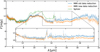 |
Fig. 1 MIRI spectrum of Sz 28 newly reduced (JWST standard pipeline version 1.13.4, orange) and as shown by Kanwar et al. (2024a) (version 1.11.1, blue). The Spitzer spectrum of the same source is shown in green. |
2.2 Observational data
The JWST/MIRI spectrum of Sz 28 reduced with version 1.11.1 of the JWST standard pipeline has been published by Kanwar et al. (2024a) who estimated the lower limit of the observational uncertainty with the Exposure Time Calculator to be 0.1 mJy. Since then several improvements to the data reduction have been made. Therefore, we show an updated spectrum (reduced with version 1.13.4, Bushouse et al. 2024) in this study (Fig. 1). While a detailed description of the data reductions is given by Kanwar et al. (2024a), we list here the improvements made. The JWST standard pipeline uses CRDS context of jwst_1215.pmap with the VIP package version 1.4.0 (Gomez Gonzalez et al. 2017; Christiaens et al. 2023). Among the improvements of the updated pipeline are a correction of the spectral leak (at about 12.2 μm) and an additional bad pixel correction leading to a higher signal-to-noise ratio. Fig. 1 illustrates the improvements of the new data reduction compared to the one used by Kanwar et al. (2024a). The overall flux levels differ due to the new calibration files. Similarly, the line widths of weak features change slightly. All of this results in changes in the retrieved molecular conditions.
2.3 Fitting procedure
We use the UltraNest package (Buchner 2021) which utilises the Monte Carlo algorithm MLFriends Buchner (2016, 2019) to derive the posterior distributions of the model parameters. This algorithm is optimised for robustness, especially for highly dimensional parameter spaces. The details are provided in the references above.
A classical Gaussian likelihood function ![$\[\mathcal{L}\]$](/articles/aa/full_html/2024/10/aa50891-24/aa50891-24-eq9.png) is used to evaluate the differences between the model spectrum Fi,model and the observations Fi,obs with uncertainties σi,obs. The index i = 1 ... Nobs enumerates all wavelength points in the selected wavelength range:
is used to evaluate the differences between the model spectrum Fi,model and the observations Fi,obs with uncertainties σi,obs. The index i = 1 ... Nobs enumerates all wavelength points in the selected wavelength range:
![$\[\mathcal{L}=\prod_{i=1}^{N_{\mathrm{obs}}} \frac{1}{\sqrt{2 \pi \sigma_{i, \mathrm{obs}}^2}} \exp \left(-\frac{\left(F_{i, \text { model }}-F_{i, \mathrm{obs}}\right)^2}{2 \sigma_{i, \mathrm{obs}}^2}\right).\]$](/articles/aa/full_html/2024/10/aa50891-24/aa50891-24-eq10.png) (1)
(1)
We derive the observational uncertainty as a free (nonlinear) parameter. This avoids a manual uncertainty determination based on line-free wavelength regions of the observation. The parameter aobs defines σi,obs as proportional to the flux of the observation,
![$\[\sigma_{i, \mathrm{obs}}=a_{\mathrm{obs}} F_{i, \mathrm{obs}}.\]$](/articles/aa/full_html/2024/10/aa50891-24/aa50891-24-eq11.png) (2)
(2)
The total flux of the model is rebinned to the observation’s wavelength points (Fi,model) using SpectRes Python package (Carnall 2017).
We adopt the approach described in Kaeufer et al. (2024) to reduce the complexity of the parameter space and, consequently, the computational cost of the retrieval process. This technique employs a non-negative least square (NNLS) solver (Virtanen et al. 2020) to determine the linear parameters namely the dust abundances, the emitting areas of each molecule, the rim, and midplane. UltraNest creates a set of non-linear parameters, while the remaining linear parameters are determined through NNLS. The total set of parameters is then used to calculate the likelihood of the model with respect to the observation. Therefore, the linear parameters are not determined in a fully Bayesian way, but their posterior is approximated. However, Kaeufer et al. (2024) shows that this significant improvement in computational speed (a factor of 80 for a mock retrieval) leaves the posterior of the molecular parameters basically unaffected, with only the uncertainties of the retrieved dust composition decreasing slightly.
3 Results
We aim to determine the molecular and the dust properties of Sz 28 based on a large wavelength region (from 4.9 μm to 17 μm) of the JWST/MIRI spectrum. For that, we need to determine the molecules relevant to describe the spectrum of Sz 28 in addition to the posterior of the retrieved parameters. We adopt an interactive process to achieve this goal. In a first Bayesian analysis we include a large number of molecules. This includes molecules already detected in Sz 28 (C2H2, HCN, C6H6, CO2, HC3N, C2H6, C3H4, C4H2, CH3, and CH4, Kanwar et al. 2024a), but also potential molecules which existence or non-existence we want to evaluate (H2O, CO, NH3, C2H4). After that, we exclude each molecule individually and evaluate the evidence for their presence using the Bayes factor (Sect. 3.1). Then, this process is repeated for the isotopologues for which we have spectroscopic data (Sect. 3.2). This selection of molecules and isotopologues results in a final fit, that only includes the detectable species, for which the molecular emission conditions are described in Sect. 3.3.
3.1 Molecule selection
The prior ranges of all free parameters that are fitted with Ultra-Nest are listed in Table 1. The dust temperature prior ranges are chosen to avoid convergence towards the prior’s edges. All priors of the power law exponents are limited between −1 and −0.1, to include known literature values (−0.6 and −0.4, and values from −0.95 to −0.5 from Brittain et al. (2023) and Fedele et al. (2016), respectively). The prior ranges of all molecular parameters are determined by the grid’s extent of the underlying slab models from Arabhavi et al. (2024).
The distance to the object is fixed to 192.2 pc (Gaia Collaboration 2021). We do not account for the inclination (i) of Sz 28 with our setup. However, an inclusion would only enlarge the retrieved emitting areas by cos i. All dust species listed in Sec. 2.1 are included with sizes of 0.1 μm, 2 μm, and 5 μm in the retrieval.
The full Bayesian run with all molecules optimises 65 parameters by UltraNest and a further 31 linear parameters by NNLS. This run finished after about 39 million model evaluations and approximately 1.64 days on 64 CPUs (~105 CPU days).
After that, we exclude every molecule individually for a new Bayesian analysis. By calculating the logarithm of the Bayes factors (ln B) from two runs, we can quantify the evidence for the presence of a molecule in the spectrum. The Bayes factor compares the global evidence for different fits. Values of ln B < 1, 1 < ln B < 2.5, 2.5 < ln B < 5, 5 < ln B < 11, and 11 < ln B can be translated to no evidence, weak evidence, moderate evidence, strong evidence, and very strong evidence, respectively, for one model over another model (Trotta 2008). The sign of ln B indicates which model is preferred. A negative value indicates that the variant model is preferred whereas a positive value of ln B indicates the same for the original model. The Bayes factor is always calculated between the retrieval including all molecules and the one excluding a single molecule at a time.
While there is very strong evidence for most species, as seen in Table 2, we examine the few cases for which the evidence is less strong. These species are H2O, NH3, CO, C2H4, and CH3.
The negative value of ln B for H2O indicates that the extra parameters for water are not worth the change in fit quality. The value of −1.95 indicates weak evidence against water. This is consistent with previous studies (Arabhavi et al. 2024; Kanwar et al. 2024a) that find a hydrocarbon-rich chemistry around VLMS that is depleted in oxygen. We discuss a possible upper limit for the H2O abundance in Sz 28 in Sec. 4.2.
There is no evidence for or against the presence of C2H4 in Sz 28 (ln B = −0.16). Analysing the retrieval including C2H4, we cannot identify a C2H4 feature in the observation. The fit opted therefore for optically thick emission instead (middle and lower left panels of Fig. 2). This is reflected in the retrieved column density range from 8 × 1022 cm−2 to 3 × 1023 cm−2. Due to the combination of the inconclusive Bayes factor and the absence of a clear feature in model and observation, we see no evidence for C2H4 in Sz 28.
CH3 produces non-significant evidence as well. As seen in the lower right panel of Fig. 2, CH3 is predicted to produce a clear feature (the Q-branch) at about 16.48 μm. The observed weakness of that feature (~0.3 mJy) explains why the Bayes factor is non-significant regarding this molecule. Additional lines of CH3 are too weak to be detected, with the lines of the P-branch that get stronger at high column densities falling beyond the analysed wavelength region (e.g. 17.6 μm). However, due to the strong visual confirmation of this molecule’s Q-branch, we include it in the further study.
The Bayes factor of CO (ln B = 0.78) indicates that the inclusion of CO does not improve the fit quality significantly. As shown by Kanwar et al. (2024a), the wavelength region that shows potential CO emission is dominated by the stellar spectrum (upper panel of Fig. 2), which shows photospheric CO absorption lines. Therefore, our fit depends on the quality and sufficient resolution of the photospheric input spectrum. As seen in Fig. 2, there is no convincing evidence for CO emission in Sz 28 and a better description of the stellar spectrum is needed to draw further conclusions.
Lastly, the Bayes factor of NH3 (ln B = 8.18) denotes strong evidence for the molecule emitting in Sz 28. Analysing the spectral features (Fig. 2), there is some overlap of NH3 features with the JWST/MIRI spectrum (e.g. the features at about 11.52 μm). However, the region is dominated by unexplained molecular features, which means that molecules that are not included in this retrieval or not included lines of examined molecules might explain the potential NH3 features as well. This can be especially seen in the second row of Fig. 2. Additionally, we retrieve very low temperatures for NH3 (from ![$\[99_{-24}^{+50} \mathrm{~K}\]$](/articles/aa/full_html/2024/10/aa50891-24/aa50891-24-eq43.png) to
to ![$\[63_{-13}^{+28} \mathrm{~K}\]$](/articles/aa/full_html/2024/10/aa50891-24/aa50891-24-eq44.png) ) together with rather high column densities (from
) together with rather high column densities (from ![$\[4_{\div 14}^{\times 6.2}(+19) ~\mathrm{cm}^{-2}\]$](/articles/aa/full_html/2024/10/aa50891-24/aa50891-24-eq45.png) to
to ![$\[8_{-7}^{+60}(+19) ~\mathrm{cm}^{-2}\]$](/articles/aa/full_html/2024/10/aa50891-24/aa50891-24-eq46.png) ). These low temperatures and high column densities are needed to reduce the strength of the features at 10.35 μm and 10.75 μm and increase the strength at 11.26 μm and 11.52 μm. We argue that all the unaccounted molecular features lead to a higher dust continuum in our retrieval. A lower continuum might allow for stronger features at 10.35 μm and 10.75 μm and therefore different parameter values. All in all, the statistical evidence for NH3 is not corroborated by visual inspection of the spectrum. This means that some evidence for NH3 exists but further analysis is needed to claim the first detection in a JWST/MIRI spectrum. We include NH3 in the further analysis due to the improvement of the fitting it provides, keeping in mind that it does not overlap strongly with other included species (as stated above C2H4 is excluded) and therefore has only a limited effect on their retrieved parameters.
). These low temperatures and high column densities are needed to reduce the strength of the features at 10.35 μm and 10.75 μm and increase the strength at 11.26 μm and 11.52 μm. We argue that all the unaccounted molecular features lead to a higher dust continuum in our retrieval. A lower continuum might allow for stronger features at 10.35 μm and 10.75 μm and therefore different parameter values. All in all, the statistical evidence for NH3 is not corroborated by visual inspection of the spectrum. This means that some evidence for NH3 exists but further analysis is needed to claim the first detection in a JWST/MIRI spectrum. We include NH3 in the further analysis due to the improvement of the fitting it provides, keeping in mind that it does not overlap strongly with other included species (as stated above C2H4 is excluded) and therefore has only a limited effect on their retrieved parameters.
Building on the results explained above, we exclude H2O, CO, and C2H4 from the further retrieval so that only the molecules with significant evidence are present. We note that excluding molecules from the fitting procedure will decrease the uncertainties of remaining molecules with overlapping wavelength regions with excluded molecules. However, comparing the posterior of the initial retrieval and the one excluding the species without significant evidence, we do not see a substantial change in retrieved parameter values and uncertainties. This hints that there are little degeneracies between the excluded and included parameters. Only the values for C2H6 change slightly, due to the molecule emitting in a similar wavelength range as the excluded C2H4.
Prior distributions of free parameters to fit Sz 28 with the full complexity model.
Bayes factors that quantify the evidence for different molecules in the JWST/MIRI spectrum of Sz 28.
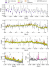 |
Fig. 2 Zoom in on the molecular features of the maximum likelihood model for CO, C2H4, CH3, and NH3. The upper panel shows the wavelength region from 4.9 μm to 5.1 μm, where CO potentially emits. The middle ranks and lower left panel display three regions that exhibit NH3 emission and a C2H4 quasi-continuum. At the lower right panel (from 16.4 μm to 16.6 μm) CH3 emission can be seen. The black line shows the JWST/MIRI spectrum of Sz 28 with the blue line indicating the continuum, visible where no molecular emission is present. |
Bayes factors that quantify the evidence for different isotopologues in the JWST/MIRI spectrum of Sz 28.
3.2 Evidence for isotopologues
Kanwar et al. (2024a) detected 13CCH2 and 13CO2 in the JWST/MIRI spectrum of Sz 28. We aim to evaluate the evidence for four isotopologues (13CH4, 13CCH6, 13CCH2, and 13CO2), similarly to the evidence for different molecules as shown in Sect. 3.1. The rarer isotopologues are not introduced as separate component, but rather as emitting under the same conditions as the main isotopologue. Therefore, they introduce no additional parameters. This is a simplification, since they are typically optically thinner, which means that deeper layer of the disk are contributing to their emission. However, this simplified treatment can account for line overlap between the main and rarer isotopologue since they are calculated in the same slab model. 13CH4 and 13CO2 are included with a ratio of 1 : 70 to the main isotopologue, with 13CCH2 and 13CCH6 having a ratio of 1 : 35 (Woods & Willacy 2009).
To quantify the evidence for isotopologues, we compare Bayesian retrievals with and without the 13C isotope. For the full run, 13CH4, 13CCH6, 13CCH2, and 13CO2 were included under the same conditions as CH4, CCH6, CCH2, and CO2, respectively. All priors are identical to the ones presented in Sect. 3.1, with the excluded molecules not being reintroduced.
The Bayes factors evaluating the evidence for the different isotopologues are listed in Table 3. There is very strong evidence for 13CH4 and 13CCH2 and strong evidence for 13CO2.
The spectral differences can be seen in Fig. 3. The upper panel shows the differences between the retrieval with (grey) and without 13CH4 (cyan). The Q-branch of 13CH4 is at about 7.7 μm. Similarly, a few of wavelength regions (e.g. at about 7.55 μm, 7.57 μm and 7.74 μm) exhibit minor differences between both versions. The Bayes factor (ln B = 16.94) reflects that all of the changes due to including 13CH4 improve the fitting quality (the posterior is moved closer to the observation). However, the poor fitting quality in this wavelength range means that no clear 13CH4 are identifiable in the JWST/MIRI spectrum. Since the number of parameters stays the same regardless of isotopologues being included, we include 13CH4 in the further analysis since it improves the fit quality, but we do not claim a detection of this isotopologue.
For 13CCH2 and 13CO2, there are clear features at 13.73 μm (third panel) and 15.41 μm (lowest panel) that are associated with the isotopologue, respectively. The versions excluding the respective isotopologues (burgundy and dark green) are therefore not able to reproduce the observed spectrum at these wavelengths.
The negative logarithm of the Bayes factor for 13CCH6 suggests that the exclusion of the isotopologue results in better overlap between the posterior of models and the observed spectrum. As seen in the second panel of Fig. 3, the posterior without 13CCH6 (light green) shows more pronounced features. This is because most 13CCH6 features are in between the features of the main isotopologue. This ‘smoothed’ spectrum is according to the Bayesian retrieval a better match (even though this is visually hard to confirm) to the observation (e.g. at 12.33 μm and 12.58 μm). However, 13CCH6 might emit under different conditions than 12CCH6 which provides an alternative explanation of the Bayes factor next to the absence of 13CCH6. Based on these results we exclude the 13CCH6 from the analysis and derive the final set of molecules and isotopologues for which we find evidence in the retrieval.
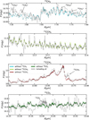 |
Fig. 3 Zoom in on the isotopologue features comparing the version with all isotopologues (grey) with the ones excluding 13CH4, 13CCH6, 13CCH2, and 13CO2, respectively. While the JWST/MIRI spectrum is shown in 1σ, 2σ, and 3σ flux levels of the posteriors are displayed in lighter growing shades of their respective colours. |
3.3 Emission conditions in Sz 28
The final retrieval incorporates the following molecules: C2H2, 13CCH2, HCN, C6H6, CO2, 13CO2, HC3N, C2H6, C3H4, C4H2, CH3, CH4,13CH4, and NH3. The isotopologue ratios are given in Sect. 3.2. This results in 53 parameters optimised by UltraNest and 28 linear parameters.
Figure 4 shows the posterior of model fluxes (blue line) and the maximum likelihood model from the posterior distribution (coloured areas). The molecular features of all molecules are clearly identifiable. The wavelength region (from about 8.5 μm to 11.5 μm) between the CH4 feature and the line-rich region displays many unidentified molecular lines next to the potentially detected weak NH3 features. C2H4 has been identified at this wavelength region in ISO-ChaI-147 to form a quasi-continuum (Arabhavi et al. 2024). However, the CH2 wagging mode (ν7) of C2H4 at 10.53 μm is not present in the JWST/MIRI spectrum of Sz 28, and the species is not found in the spectrum according to the Bayes factor. Therefore, we speculate that other molecules not present in this analysis or missing lines of included molecules might be responsible for these features. Kanwar et al. (2024a) provide a list of hydrocarbons that are chemically expected, but for which no mid-infrared spectral data is available in the HITRAN (Gordon et al. 2022) and GEISA (Delahaye et al. 2021) data collection. These could be candidates for the unaccounted features between 8.5 μm and 11.5 μm.
The line-rich region longwards of ~ 11.5 μm is dominated by strong C2H2 features. We identify a quasi-continuum of C4H2 between about 15.5 μm and 16.5 μm, which differs from the results by Kanwar et al. (2024a). The previous study fitted this region with a stronger dust continuum and postulated three scenarios to explain potential mismatches (we investigate this in Sect. 4.3). At wavelengths longwards of the CH3 feature (at about 16.5 μm), there is little molecular emission in the model that explains the observed spectral lines. We attribute this to missing molecules and missing lines in the spectral data of included molecules (e.g. missing lines of CH3).
Next, we focus on the retrieved molecular and dust temperature properties which are listed with their uncertainties in Table 4. The relevant radial emitting area of all the molecules is determined by the central 70% of radial flux emission, as described by Kaeufer et al. (2024). The parameters with a 0.15 and 0.85 subscript denote the inner and outer edges of this region. The emitting areas are provided as the radii of disks with the same area. We calculate the radii (reff) using the inner (r0.15) and outer r0.85 radius of significant emission:
![$\[r_{\mathrm{eff}}^2=r_{0.85}^2-r_{0.15}^2.\]$](/articles/aa/full_html/2024/10/aa50891-24/aa50891-24-eq47.png) (3)
(3)
The molecular properties are visualised in Fig. 5 with the slab parameters from Kanwar et al. (2024a) shown for comparison. Kanwar et al. (2024a) fitted C2H2, C6H6, C4H2, and C3H4 and detected CH4, C2H6, HCN, CH3, CO2, and HC3N. It is worth noting that the differences between both studies arise from the different fitting strategies (e.g. the wavelength windows and sequential fitting employed by Kanwar et al. 2024a) and from the new data reduction of the JWST/MIRI spectrum (Sect. 2.2).
Focussing on the four molecules fitted by Kanwar et al. (2024a), we identify that the emission conditions of C2H2 and C6H6 overlap well within the error bars between both studies. However, we find lower temperatures and higher column densities for C4H2 and C3H4 compared to Kanwar et al. (2024a). This can be explained by the quasi-continuum of C4H2 that we identify in contrast to the previous study. We evaluate the robustness of this finding in Sect. 4.3.
Generally, the retrieved molecular conditions for some molecules are well constrained (e.g. CO2, C6H6, C4H2, C2H6, and CH4). This means that there is little ambiguity in which molecular conditions are able to reproduce the observed spectrum. It also means that the emission is originating from relatively homogenous regions. On the other hand, some molecules (most prominently CH3) have poorly constrained emission conditions. This is in line with our earlier conclusion that there is little evidence for CH3 in the observed spectrum which makes it more difficult to pin down the CH3 parameters.
It strikes that HCN is emitting at higher temperatures (from ![$\[695_{-40}^{+35} \mathrm{~K}\]$](/articles/aa/full_html/2024/10/aa50891-24/aa50891-24-eq48.png) to
to ![$\[820_{-40}^{+70} \mathrm{~K}\]$](/articles/aa/full_html/2024/10/aa50891-24/aa50891-24-eq49.png) ) than the rest of the molecules (≲400 K). This hints that HCN is emitting in a different region of Sz 28 which we further investigate in Sect. 4.1.
) than the rest of the molecules (≲400 K). This hints that HCN is emitting in a different region of Sz 28 which we further investigate in Sect. 4.1.
NH3, C2H6, and C3H4 show very low retrieved temperatures (upper limits of ![$\[110_{-40}^{+80} \mathrm{~K}, 100_{-16}^{+24} \mathrm{~K}\]$](/articles/aa/full_html/2024/10/aa50891-24/aa50891-24-eq141.png) , and
, and ![$\[64_{-14}^{+60} \mathrm{~K}\]$](/articles/aa/full_html/2024/10/aa50891-24/aa50891-24-eq142.png) , respectively). To reproduce the observed features with these low-temperature models, high column densities and emitting areas are needed. This is reflected in the total number of emitting molecules listed in Table 4. While the posterior median molecule numbers for NH3, C2H6, and C3H4 are all about 1049, the −1σ limits are 2 × 1045, 6.5 × 1047, 6 × 1044, respectively. This suggests that models with an extremely high number of molecules might explain the observation best, but warmer models with much fewer molecules are also possible. We tested this hypothesis by running another retrieval, limiting the emitting areas to a maximum radius of 2 au. Consequently, the emitting areas decrease and temperatures rise (see Table A.1). The restriction has no strong effect on the retrieved fit quality (ln B = 4.98, see also Fig. A.1), showing that the huge emitting areas and low temperatures from a free retrieval are not the only options to explain the JWST/MIRI spectrum of Sz 28.
, respectively). To reproduce the observed features with these low-temperature models, high column densities and emitting areas are needed. This is reflected in the total number of emitting molecules listed in Table 4. While the posterior median molecule numbers for NH3, C2H6, and C3H4 are all about 1049, the −1σ limits are 2 × 1045, 6.5 × 1047, 6 × 1044, respectively. This suggests that models with an extremely high number of molecules might explain the observation best, but warmer models with much fewer molecules are also possible. We tested this hypothesis by running another retrieval, limiting the emitting areas to a maximum radius of 2 au. Consequently, the emitting areas decrease and temperatures rise (see Table A.1). The restriction has no strong effect on the retrieved fit quality (ln B = 4.98, see also Fig. A.1), showing that the huge emitting areas and low temperatures from a free retrieval are not the only options to explain the JWST/MIRI spectrum of Sz 28.
The dust temperature structure is well constrained, except for the maximum temperature of the midplane and surface layer. We suspect that the maximum temperatures of both components have an insignificant effect on the flux in the observed wavelength region. This is why they are mostly constrained by their priors which can lead to the unphysical situations that the rim temperature is lower than the maximum temperature of midplane and surface layer. Therefore, these values are not analysed in detail. The minimum temperature of both components and the rim temperature are however well constrained (within about 10 K). The power law indices for the midplane, surface, and molecular layer are on the shallow end of the prior range and within each other’s uncertainties. Therefore, it is possible that the dust and molecular emission trace a similar disk layer, but a more in-depth analysis is needed to confirm this. Additionally, we note that the high dust temperatures compared to the temperatures of molecules such as NH3, C3H4, and C2H6 mean that if interactions between the different model components would be included in the model, gas absorption features might appear (as discussed in Sect. 2.1).
The derived observational uncertainty (aobs) of ![$\[1.436_{-0.011}^{+0.010} \%\]$](/articles/aa/full_html/2024/10/aa50891-24/aa50891-24-eq143.png) together with the mean observational flux of 11 mJy translates into an uncertainty of 0.16 mJy which is slightly larger than the uncertainty of about 0.1 mJy estimated with the Exposure Time Calculator (Kanwar et al. 2024a). This is expected since aobs resembles the observed uncertainty that best explains the difference between models and observations. Therefore, the many unidentified lines between 9 μm and 12 μm increase aobs. Fixing the observed uncertainty to 1% of the observed flux results in a nearly identical posterior distribution compared to the treatments of the uncertainty as a free parameter. Therefore, the retrieval of the uncertainty eliminates the need to fix this parameter without any significant change regarding the retrieved distribution for all other parameters.
together with the mean observational flux of 11 mJy translates into an uncertainty of 0.16 mJy which is slightly larger than the uncertainty of about 0.1 mJy estimated with the Exposure Time Calculator (Kanwar et al. 2024a). This is expected since aobs resembles the observed uncertainty that best explains the difference between models and observations. Therefore, the many unidentified lines between 9 μm and 12 μm increase aobs. Fixing the observed uncertainty to 1% of the observed flux results in a nearly identical posterior distribution compared to the treatments of the uncertainty as a free parameter. Therefore, the retrieval of the uncertainty eliminates the need to fix this parameter without any significant change regarding the retrieved distribution for all other parameters.
 |
Fig. 4 Molecular emission of the maximum likelihood model of Sz 28. The JWST/MIRI spectrum is shown in black. The median flux of the posterior models is shown in blue with the 1σ, 2σ, and 3σ flux levels being displayed in lighter colours. The cumulative contributions of all included molecules are shown in different colours. |
Posterior parameter values and uncertainties for selected parameters of the Sz 28 fit.
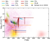 |
Fig. 5 Molecular emission properties of Sz 28. The different coloured areas denote where the respective molecule emits significantly in the posterior of models. The errorbars indicate the molecular emission conditions determined by Kanwar et al. (2024a). |
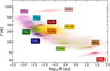 |
Fig. 6 Radial molecular emission regions of Sz 28. The different coloured areas denote where the respective molecule emits significantly in the posterior of models. |
4 Discussion
4.1 Emission location
The molecular flux in DuCKLinG is described by a 1D radial structure of temperature and column density. After having discussed the temperature and column density ranges in the previous section, we now have a closer look at the radial regions from which the molecules emit. As shown in Sect. 2.1, the emission of every molecule follows a radial power law in temperature and column density. The temperature decreases radially (due to the prior of qemis in Table 1), but the column density can increase or decrease based on ∑tmax and ∑tmin. Fig. 6 indicates the regions from which the molecules emit significantly (between t0.85 and t0.15).
We estimate the stellar radius of Sz 28 based on premainsequence evolutionary tracks from Siess et al. (2000), an effective temperature of 3060 K, and a luminosity of 0.04 L⊙ to be 0.0025 au which corresponds to a log10 value of the radius of −2.6. Therefore, the stellar radius is at about the left edge of Fig. 6.
It can be seen that the emissions of all molecules except for HCN form a radial power law in temperature. We stress that this is not an input to the model. We condition all molecules to have the same power law index (qemis), but the temperatures at the same radius are allowed to differ. The retrieved radial power law might indicate that the molecules are emitted from a similar layer of the disk instead of different depths at the same radius.
The emission of HCN does not align with all other molecules. The high temperatures (from about 800 K to 700 K) are present at radii from about 0.1 au to 1 au. However, the column densities of about 1014 cm−2 result in the lowest number of emitting molecules ![$\[\left(5.1_{-0.4}^{+0.4}(+40)\right)\]$](/articles/aa/full_html/2024/10/aa50891-24/aa50891-24-eq144.png) of all examined species. The high temperatures and low column densities at relatively large radii suggest that HCN is emitted in an upper layer of the disk. Woitke et al. (2024) find most of the emission of HCN to originate close to the midplane in a thermo-chemical model describing the JWST/MIRI spectrum of Ex Lup. However, lower concentrations of the molecule are also present in a higher radially extended layer, which might explain the emission of HCN in the case of Sz 28. Earlier Spitzer results also generally find high temperatures (≳700 K) of HCN in T Tauri and Herbig disks (Salyk et al. 2011).
of all examined species. The high temperatures and low column densities at relatively large radii suggest that HCN is emitted in an upper layer of the disk. Woitke et al. (2024) find most of the emission of HCN to originate close to the midplane in a thermo-chemical model describing the JWST/MIRI spectrum of Ex Lup. However, lower concentrations of the molecule are also present in a higher radially extended layer, which might explain the emission of HCN in the case of Sz 28. Earlier Spitzer results also generally find high temperatures (≳700 K) of HCN in T Tauri and Herbig disks (Salyk et al. 2011).
As noted before, C2H6, NH3, and C3H4 emit at very low temperatures from large emission areas. As detailed in Sect. 3.3, the posteriors of these molecules extend to smaller emitting areas and limiting the emitting radii to less than 2 au does not significantly impact the fit quality.
CH3 is rather poorly constrained. Therefore, we are not analysing the radial behaviour in detail. CO2, CH4, C2H2, C4H2, and C6H6 emit at well-defined very similar radial regions. Therefore, we have good reasons to assume that these molecules are co-spatial in this disk. The mean temperature in a radial range between 0.02 au and 0.2 au of CO2 (220 K), C4H2 (160 K), and C6H6 (180 K) are slightly lower than the temperatures of CH4 (350 K) and C2H2 (290 K), suggesting that CO2 and C4H2 emit slightly deeper in the disk or in the case of C6H6 at slightly larger radii (Fig. 6). HC3N originates potentially from the same region but extends to larger radii. The full thermo-chemical disk models with ProDiMo for Sz 28 by Kanwar et al. (2024a) suggest that the inner disk must have a high C/O ratio to explain the large abundances of the hydrocarbon molecules. A chemically consistent solution to the presence of CO2 along with hydrocarbons can be a non-co-spatial origin in case of C/O≫ 2 (Kanwar et al. 2024b). However, for moderate C/O ≈ 2 it can be co-spatial (Kanwar et al. 2024a), and for close to solar C/O = 0.46 it can as well, see ProDiMo models for EX Lupi (Woitke et al. 2024).
In the latter model, the irradiation of the inner disk by X-rays unlocks the CO on timescales of a few years, and the liberated oxygen and carbon atoms react quickly to form C2H2 and HCN that are co-spatial with CO2, although the line emission region for CO2 results to be situated at slightly larger radii compared to C2H2 and HCN, which is different from the results of our retrieval models presented in this paper. The ProDiMo models for both objects show that the emission lines from HCN and C2H2 originate in similar disk layers, which is also different from the results found in this paper.
Temmink et al. (2024) find that HCN, C2H2, and CO2 are emitting at increasing depths in the disk of the T Tauri star DR Tau. We can confirm this behaviour for the disk of Sz 28, with the three molecules showing decreasing emitting temperatures at similar radii.
4.2 Constraining the water abundance in Sz 28
There is no evidence for water in the JWST/MIRI spectrum of Sz 28 (according to the Bayes factor presented in Sect. 3.1). This led us to determine an upper limit for the water abundance. We estimated this limit by selecting slab models from the grid presented by Arabhavi et al. (2024) that result in peak fluxes below 3σ of the noise level of Sz 28 (0.1 mJy, Kanwar et al. 2024a).
Figure 7 shows the column densities of water for given temperatures and emitting areas (characterised by the radius of this area) that result in peak fluxes below 0.3 mJy in the fitted wavelength range of Sz 28. At high temperatures (≳ 600 K), when assuming large emitting areas (reff ≳ 1 au), even the lowest examined column densities (1014 cm−2) are detectable for Sz 28. If the water emission temperature is only 200 K, again assuming an emitting radius of 1 au, the upper limit for the water column density is about 2 × 1017 cm−2. This shows that small but substantial amounts of water could be hidden in the disk of Sz 28 without producing noticeable signals. Previous findings for the VLMS J160532, that column densities of 3 × 1018 cm−2 are not detectable if H2O is emitting under the same conditions as C2H2, support our conclusion (Tabone et al. 2023). This phenomenon of water as a weak emitter compared to hydrocarbons is examined in further detail by Arabhavi et al. (in prep).
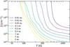 |
Fig. 7 Column densities of water for given temperatures (horizontal axis) and emitting radii (colour) that result in peak fluxes of 3σ of the noise of the JWST/MIRI observation of Sz 28. |
4.3 Evidence for a C4H2 quasi-continuum
The most significant difference in the retrieved molecular emission between our study and Kanwar et al. (2024a) is the C4H2 quasi-continuum from about 15.5 μm to 16.4 μm. Kanwar et al. (2024a) proposed three scenarios to explain the mismatches at these wavelengths of their fit: missing dust species, incomplete opacity data, or a molecular quasi-continuum. Using the Bayesian approach in our study we can quantify the evidence for this quasi-continuum. We investigate the C4H2 properties in two ways. First, we show how limiting the integrated flux of C4H2 affects the retrieval. Secondly, we examine if the dust continuum at about 15.5 μm to 16.4 μm is a consequence of the continuum at shorter wavelengths or the best solution for the line-rich region from ~ 12.0 μm onwards as well. This latter case would mean that fitting the wavelength region from 12 μm to 17 μm should result in the same quasi-continuum.
The first retrieval uses the same priors and settings as the final run presented in Sec. 3.3. Additionally, we constrain the integrated flux of C4H2 to be below 4.5 × 10⁻¹⁹ W/m2 by setting the likelihood of higher integrated fluxes to highly unlikely values. This limit is about the C4H2 flux between 15.85 μm and 15.95 μm from the maximum likelihood model without any constraints. The restriction excludes the possibility of a C4H2 quasi-continuum while still allowing for C4H2 emission to describe the features at about 15.9 μm. Analysing the newly retrieved parameters, we find that the values for C4H2 (column density range from ![$\[3.1_{-1.9}^{+5}(+16) ~\mathrm{cm}^{-2}\]$](/articles/aa/full_html/2024/10/aa50891-24/aa50891-24-eq145.png) to
to ![$\[4.5_{-3.5}^{+17}(+17) ~\mathrm{cm}^{-2}\]$](/articles/aa/full_html/2024/10/aa50891-24/aa50891-24-eq146.png) and a temperature range from
and a temperature range from ![$\[210_{-80}^{+80} \mathrm{~K}\]$](/articles/aa/full_html/2024/10/aa50891-24/aa50891-24-eq147.png) to
to ![$\[117_{-33}^{+50} \mathrm{~K}\]$](/articles/aa/full_html/2024/10/aa50891-24/aa50891-24-eq148.png) ) fall within the retrieved values from Kanwar et al. (2024a). However, the temperature for C3H4 stays very low (≲100 K) with the column density reaching a maximum value of
) fall within the retrieved values from Kanwar et al. (2024a). However, the temperature for C3H4 stays very low (≲100 K) with the column density reaching a maximum value of ![$\[8.6_{-1.9}^{+1.1}(+23) ~\mathrm{cm}^{-2}\]$](/articles/aa/full_html/2024/10/aa50891-24/aa50891-24-eq149.png) . The middle panel of Fig. 8 shows the wavelength region of the C4H2 quasi-continuum for the new retrieval. It can be seen that limiting the molecular flux from C4H2 results in more flux from C3H4 with the dust continuum only increasing slightly in flux (comparing the upper and middle panel). However, this new fitting quality is significantly worse compared to the unconstrained fit. For example, there are large underpredictions in the wavelength region from 16.1 μm to 16.3 μm. Additionally, C3H4 is producing a strong feature at about 16.4 μm that is not mirrored in the observation. All of this is reflected in the logarithm of the Bayes factor of 58.82 between the original (unconstrained) and limited fit. Even though the Bayes factor for this exercise is positive by definition (same prior ranges, but a likelihood penalty for the limited fit), the large value indicates very strong evidence for the unconstrained fit. This makes us confident, that the quasi-continuum of C4H2 cannot easily be replaced by other molecular emissions or a higher dust continuum if examining the full wavelength range.
. The middle panel of Fig. 8 shows the wavelength region of the C4H2 quasi-continuum for the new retrieval. It can be seen that limiting the molecular flux from C4H2 results in more flux from C3H4 with the dust continuum only increasing slightly in flux (comparing the upper and middle panel). However, this new fitting quality is significantly worse compared to the unconstrained fit. For example, there are large underpredictions in the wavelength region from 16.1 μm to 16.3 μm. Additionally, C3H4 is producing a strong feature at about 16.4 μm that is not mirrored in the observation. All of this is reflected in the logarithm of the Bayes factor of 58.82 between the original (unconstrained) and limited fit. Even though the Bayes factor for this exercise is positive by definition (same prior ranges, but a likelihood penalty for the limited fit), the large value indicates very strong evidence for the unconstrained fit. This makes us confident, that the quasi-continuum of C4H2 cannot easily be replaced by other molecular emissions or a higher dust continuum if examining the full wavelength range.
To examine whether a more flexible dust continuum can replace the C4H2 quasi-continuum, we exclude the observations shortwards of 12 μm from the analysis. There is theoretical (Jang et al. 2024) and observational (Kessler-Silacci et al. 2006) evidence that the dust composition changes within a disk resulting in different wavelength regions probing different dust compositions. Since we do not account for radial changes in dust properties in our 1D model, focussing on small wavelength ranges is an alternative to allow for dust composition gradients. The lower panel of Fig. 8 illustrates the maximum likelihood model of the retrieval from 12 μm to 17 μm with the same priors and settings as mentioned in Sec. 3.3. The resulting molecular fluxes are very similar to the one shown in Fig. 4. The retrieved parameters for C4H2 (column density from ![$\[1.6_{\div 505}^{\times6.0}(+18) ~\mathrm{cm}^{-2}\]$](/articles/aa/full_html/2024/10/aa50891-24/aa50891-24-eq150.png) to
to ![$\[2.2_{-1.9}^{+10}(+19) ~\mathrm{cm}^{-2}\]$](/articles/aa/full_html/2024/10/aa50891-24/aa50891-24-eq151.png) with a temperature from
with a temperature from ![$\[236_{-33}^{+40} \mathrm{~K}\]$](/articles/aa/full_html/2024/10/aa50891-24/aa50891-24-eq152.png) to
to ![$\[183_{-33}^{+32} \mathrm{~K}\]$](/articles/aa/full_html/2024/10/aa50891-24/aa50891-24-eq153.png) ) show a slight increase in temperature with a coinciding decrease in column density. Therefore, they are again closer to the values retrieved by Kanwar et al. (2024a) but still show a quasi-continuum. This illustrates that the changes in retrieved conditions between both studies might partly be due to differences in the dust continuum. Summarising, the persistence of a C4H2 quasi-continuum shows that it is not a consequence of a restricted dust continuum fit over the short wavelength region but indeed the best-fitting solution for this molecular line-rich wavelength region.
) show a slight increase in temperature with a coinciding decrease in column density. Therefore, they are again closer to the values retrieved by Kanwar et al. (2024a) but still show a quasi-continuum. This illustrates that the changes in retrieved conditions between both studies might partly be due to differences in the dust continuum. Summarising, the persistence of a C4H2 quasi-continuum shows that it is not a consequence of a restricted dust continuum fit over the short wavelength region but indeed the best-fitting solution for this molecular line-rich wavelength region.
Both of these tests lead to the same finding of a C4H2 quasi-continuum that is robust and not easily replaceable by other emissions or a change of continuum in our model. This nicely illustrates the benefit of a simultaneous fit of all molecules and the dust continuum.
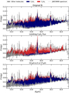 |
Fig. 8 Zoom in to the C4H2 quasi-continuum of the maximum likelihood model for the retrieval presented in Sec. 3.3 (upper panel), the retrieval restricting the C4H2 flux (middle panel), and for the retrieval focussing only on the wavelength region from 12 μm to 17 μm (lower panel). The JWST/MIRI spectrum of Sz 28 is shown in black, with the molecular contributions to the maximum likelihood model being shown in different colours. |
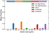 |
Fig. 9 Mass fraction of the optically thin dust. The histograms indicate the median retrieved mass fraction of every dust species (composition and size), with the error bars denoting the 16th and 84th percentile. The dust composition is indicated by colour with the size displayed on the x-axis. |
4.4 Dust composition
Next to the gas properties, DuCKLinG allows for the retrieval of the dust composition. Fig. 9 illustrates the dust mass fraction for all species (composition and sizes) used in the fitting procedure.
For all grain compositions (except for Silica), the largest grain size (5 μm) is the most common component. Additionally, ![$\[44.7_{-2.1}^{+2.1} \%\]$](/articles/aa/full_html/2024/10/aa50891-24/aa50891-24-eq154.png) of the optically thin dust is crystalline. Both factors indicate that the dust in Sz 28 is highly evolved. The same conclusion is drawn for Sz 28 by Kanwar et al. (2024a), even though the detailed numbers (crystalline fraction of ~20%) differ. These minor differences can be due to, for example, the new data reduction of the JWST/MIRI spectrum but also the different wavelength regions considered in both studies. While Kanwar et al. (2024a) fitted the dust continuum in two wavelength regions (from 4.9 μm to 15 μm and from 15 μm to 22 μm) by an iterative process between dust and gas fitting, our study investigates the region from 4.9 μm to 17 μm with a single set of dust (and gas) parameters. As mentioned before, different wavelength regions probe the dust composition at different disk positions. We conclude from both studies that describing the dust with a single composition up to 17 μm is feasible, while larger wavelength regions require gradients in the dust compositions.
of the optically thin dust is crystalline. Both factors indicate that the dust in Sz 28 is highly evolved. The same conclusion is drawn for Sz 28 by Kanwar et al. (2024a), even though the detailed numbers (crystalline fraction of ~20%) differ. These minor differences can be due to, for example, the new data reduction of the JWST/MIRI spectrum but also the different wavelength regions considered in both studies. While Kanwar et al. (2024a) fitted the dust continuum in two wavelength regions (from 4.9 μm to 15 μm and from 15 μm to 22 μm) by an iterative process between dust and gas fitting, our study investigates the region from 4.9 μm to 17 μm with a single set of dust (and gas) parameters. As mentioned before, different wavelength regions probe the dust composition at different disk positions. We conclude from both studies that describing the dust with a single composition up to 17 μm is feasible, while larger wavelength regions require gradients in the dust compositions.
The crystallinity fraction of more than 40% is consistent with findings for other VLMS (Apai et al. 2005). This high fraction is mostly driven by the abundances of forsterite and enstatite with grain sizes of 5 μm. To test if these grains are needed to describe the observation, we run an additional retrieval excluding them. The Bayes factor (lnB = 36) between the fit including all dust species and the one without forsterite and enstatite with grain sizes of 5 μm provides very strong evidence that these grains are indeed necessary to sufficiently describe the observation. Interestingly, we find very similar sizes and a similar ratio of pyroxene to olivine in the crystalline and amorphous silicate components.
The effect of the dust composition on the spectrum can be seen in Fig. 10. The grains of size 5 μm exhibit the strongest influence on the dust spectrum. The total continuum follows neatly the JWST/MIRI spectrum up to about 11.5 μm. Longwards of that, the molecular emission contributes strongly to the total flux. This highlights again the difficulty disentangling the dust and gas contributions of JWST/MIRI spectra.
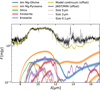 |
Fig. 10 Spectrum of the different dust compositions (colour) and sizes (line style) compared to the total dust continuum (olive; star, rim, midplane, and surface layer) and the JWST/MIRI spectrum of Sz 28 (black). Both are offset by −9 mJy. The error tubes denote the 16th and 84th percentile of the dust flux from the posterior of models. |
5 Summary and conclusion
In this paper, we analysed the dust and gas composition of Sz 28 simultaneously in a Bayesian way. This has been done using the 1D DuCKLinG model that describes the dust and gas at the same time. Sz 28 is a VLMS exhibiting many molecular features on top of dust features which complicates the fitting process. The main findings are listed below:
We confirm the previous identification by Kanwar et al. (2024a) of C2H2, HCN, C6H6, CO2, HC3N, C2H6, C3H4, C4H2, CH4, and CH3 in the disk of Sz 28. We quantify the confidence in these detections as very strong evidence for all molecules except for CH3;
There is no evidence for water emission in the JWST/MIRI spectrum of Sz 28 up to 17 μm. However, we estimate that it is possible to hide large quantities of H2O in the noise of the spectrum. For example, at a temperature of 200 K assuming an emitting areas with a radius of 1 au, the upper limit for the water column density is about 2 × 1017 cm−2;
We find tentative hints for the presence of NH3. While there is statistical evidence for this tentative detection, the wavelength region that exhibits NH3 features is dominated by unexplained lines. Therefore, other molecules that are not included in this analysis might explain the features as well;
The isotopologues 13CO2 and 13CCH2 are clearly identified in the spectrum. The signatures for 13CH4 and 13CCH6 are not clearly visible and need further investigation
HCN is emitting under higher temperatures (from
![$\[695_{-40}^{+35} \mathrm{~K}\]$](/articles/aa/full_html/2024/10/aa50891-24/aa50891-24-eq155.png) to
to ![$\[820_{-40}^{+70} \mathrm{~K}\]$](/articles/aa/full_html/2024/10/aa50891-24/aa50891-24-eq156.png) ) than all other detected molecules (≲400 K). We speculate that HCN is emitting from a radially extended upper disk layer, while all other molecules are roughly following a common temperature power law of radial emission;
) than all other detected molecules (≲400 K). We speculate that HCN is emitting from a radially extended upper disk layer, while all other molecules are roughly following a common temperature power law of radial emission;The molecular emission conditions are well constrained for CO2, C6H6, C4H2, C2H6, and CH4, with C2H2 being well constrained in temperature only and especially CH3 being poorly determined. In our retrieval, CO2 is emitting roughly co-spatially with other hydrocarbon molecules;
A C4H2 quasi-continuum from about 15.5 μm to 16.4 μm is robustly identified;
The optically thin dust of Sz 28 consists mainly of large grains (5 μm) and shows a high crystallinity fraction (~45%) hinting at highly evolved dust in Sz 28.
Acknowledgements
We acknowledge funding from the European Union H2020-MSCA-ITN-2019 under grant agreement no. 860470 (CHAMELEON).
Appendix A Retrieval with restricted emitting areas
The retrieval presented in Sec. 3.3 results in low temperatures from large emitting areas for NH3, C2H6, and C3H4. To test the robustness of this solution, we reran the retrieval (with the same settings and priors) with an additional restriction on the emitting area. By setting the likelihood function to highly unlikely values for solutions with reff > 2 au, we excluded these cases from the retrieval. The extracted parameters are listed in Table A.1, with the fluxes from the posterior of models with their molecular contribution shown in Fig. A.1. As discussed in Section 3.3, the restricted retrieval (Fig. A.1) is able to describe the JWST/MIRI spectrum of Sz 28 with a similar fitting quality as the unrestricted fit (Fig. 4). This shows that solutions with smaller emitting areas are possible.
Posterior parameter values and uncertainties for selected parameters of the Sz 28 fit for the retrieval restricted to reff ≤ 2 au.
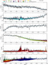 |
Fig. A.1 Molecular emission of the maximum likelihood model of Sz 28 for the retrieval restricted to reff ≤ 2 au. The JWST/MIRI spectrum is shown in black. The median flux of the posterior models is shown in blue with the 1σ, 2σ, and 3σ flux levels being displayed in lighter colours. The cumulative contributions of all included molecules are shown in different colours. |
References
- Apai, D., Pascucci, I., Bouwman, J., et al. 2005, Science, 310, 834 [NASA ADS] [CrossRef] [Google Scholar]
- Arabhavi, A. M., Kamp, I., Henning, T., et al. 2024, Science, 384, 1086 [NASA ADS] [CrossRef] [Google Scholar]
- Brittain, S. D., Kamp, I., Meeus, G., Oudmaijer, R. D., & Waters, L. B. F. M. 2023, Space Sci. Rev., 219, 7 [NASA ADS] [CrossRef] [Google Scholar]
- Brott, I., & Hauschildt, P. H. 2005, in ESA Special Publication, 576, The Three-Dimensional Universe with Gaia, eds. C. Turon, K. S. O’Flaherty, & M. A. C. Perryman, 565 [Google Scholar]
- Buchner, J. 2016, Statist. Comput., 26, 383 [NASA ADS] [CrossRef] [Google Scholar]
- Buchner, J. 2019, PASP, 131, 108005 [Google Scholar]
- Buchner, J. 2021, J. Open Source Softw., 6, 3001 [CrossRef] [Google Scholar]
- Bushouse, H., Eisenhamer, J., Dencheva, N., et al. 2024, ASP Conf. Ser., 527, 583 [NASA ADS] [Google Scholar]
- Carnall, A. C. 2017, arXiv e-prints, [arXiv:1705.05165] [Google Scholar]
- Carr, J. S., & Najita, J. R. 2011, ApJ, 733, 102 [NASA ADS] [CrossRef] [Google Scholar]
- Christiaens, V., Gonzalez, C., Farkas, R., et al. 2023, J. Open Source Softw., 8, 4774 [NASA ADS] [CrossRef] [Google Scholar]
- Delahaye, T., Armante, R., Scott, N. A., et al. 2021, J. Mol. Spectrosc., 380, 111510 [NASA ADS] [CrossRef] [Google Scholar]
- Dorschner, J., Begemann, B., Henning, T., Jäger, C., & Mutschke, H. 1995, A&A, 300, 503 [NASA ADS] [Google Scholar]
- Draine, B. T., & Flatau, P. J. 2013, arXiv e-prints [arXiv:1305.6497] [Google Scholar]
- Fedele, D., van Dishoeck, E. F., Kama, M., Bruderer, S., & Hogerheijde, M. R. 2016, A&A, 591, A95 [NASA ADS] [CrossRef] [EDP Sciences] [Google Scholar]
- Gaia Collaboration (Brown, A. G. A., et al.) 2021, A&A, 649, A1 [NASA ADS] [CrossRef] [EDP Sciences] [Google Scholar]
- Gasman, D., van Dishoeck, E. F., Grant, S. L., et al. 2023, A&A, 679, A117 [NASA ADS] [CrossRef] [EDP Sciences] [Google Scholar]
- Gomez Gonzalez, C. A., Wertz, O., Absil, O., et al. 2017, AJ, 154, 7 [Google Scholar]
- Gordon, I. E., Rothman, L. S., Hargreaves, R. J., et al. 2022, J. Quant. Spec. Radiat. Transf., 277, 107949 [NASA ADS] [CrossRef] [Google Scholar]
- Grant, S. L., van Dishoeck, E. F., Tabone, B., et al. 2023, ApJ, 947, L6 [NASA ADS] [CrossRef] [Google Scholar]
- Grynko, Y., & Shkuratov, Y. 2003, J. Quant. Spec. Radiat. Transf., 78, 319 [NASA ADS] [CrossRef] [Google Scholar]
- Henning, T., & Mutschke, H. 1997, A&A, 327, 743 [NASA ADS] [Google Scholar]
- Henning, T., & Stognienko, R. 1996, A&A, 311, 291 [NASA ADS] [Google Scholar]
- Jäger, C., Molster, F. J., Dorschner, J., et al. 1998, A&A, 339, 904 [NASA ADS] [Google Scholar]
- Jang, H., Waters, R., Kamp, I., & Dullemond, C. P. 2024, A&A, 687, A275 [NASA ADS] [CrossRef] [EDP Sciences] [Google Scholar]
- Juhász, A., Henning, T., Bouwman, J., et al. 2009, ApJ, 695, 1024 [CrossRef] [Google Scholar]
- Juhász, A., Bouwman, J., Henning, T., et al. 2010, ApJ, 721, 431 [Google Scholar]
- Kaeufer, T., Min, M., Woitke, P., Kamp, I., & Arabhavi, A. M. 2024, A&A, 687, A209 [NASA ADS] [CrossRef] [EDP Sciences] [Google Scholar]
- Kanwar, J., Kamp, I., Jang, H., et al. 2024a, A&A, 689, A231 [NASA ADS] [CrossRef] [EDP Sciences] [Google Scholar]
- Kanwar, J., Kamp, I., Woitke, P., et al. 2024b, A&A, submitted [Google Scholar]
- Kessler-Silacci, J., Augereau, J.-C., Dullemond, C. P., et al. 2006, ApJ, 639, 275 [NASA ADS] [CrossRef] [Google Scholar]
- Liebert, J., & Probst, R. G. 1987, ARA&A, 25, 473 [Google Scholar]
- Manara, C. F., Testi, L., Herczeg, G. J., et al. 2017, A&A, 604, A127 [NASA ADS] [CrossRef] [EDP Sciences] [Google Scholar]
- Ment, K., & Charbonneau, D. 2023, AJ, 165, 265 [NASA ADS] [CrossRef] [Google Scholar]
- Min, M., Waters, L. B. F. M., de Koter, A., et al. 2007, A&A, 462, 667 [NASA ADS] [CrossRef] [EDP Sciences] [Google Scholar]
- Mollière, P., Molyarova, T., Bitsch, B., et al. 2022, ApJ, 934, 74 [CrossRef] [Google Scholar]
- Muñoz-Romero, C. E., Öberg, K. I., Banzatti, A., et al. 2024, ApJ, 964, 36 [CrossRef] [Google Scholar]
- Mutschke, H., Min, M., & Tamanai, A. 2009, A&A, 504, 875 [NASA ADS] [CrossRef] [EDP Sciences] [Google Scholar]
- Öberg, K. I., Murray-Clay, R., & Bergin, E. A. 2011, ApJ, 743, L16 [Google Scholar]
- Pascucci, I., Apai, D., Luhman, K., et al. 2009, ApJ, 696, 143 [Google Scholar]
- Pascucci, I., Herczeg, G., Carr, J. S., & Bruderer, S. 2013, ApJ, 779, 178 [NASA ADS] [CrossRef] [Google Scholar]
- Sabotta, S., Schlecker, M., Chaturvedi, P., et al. 2021, A&A, 653, A114 [NASA ADS] [CrossRef] [EDP Sciences] [Google Scholar]
- Salyk, C., Pontoppidan, K. M., Blake, G. A., Najita, J. R., & Carr, J. S. 2011, ApJ, 731, 130 [Google Scholar]
- Schwarz, K. R., Henning, T., Christiaens, V., et al. 2024, ApJ, 962, 8 [NASA ADS] [CrossRef] [Google Scholar]
- Servoin, J. L., & Piriou, B. 1973, Phys. Stat. Sol. (b), 55, 677 [CrossRef] [Google Scholar]
- Shkuratov, Y. G., & Grynko, Y. S. 2005, Icarus, 173, 16 [NASA ADS] [CrossRef] [Google Scholar]
- Siess, L., Dufour, E., & Forestini, M. 2000, A&A, 358, 593 [Google Scholar]
- Tabone, B., Bettoni, G., van Dishoeck, E. F., et al. 2023, Nat. Astron., 7, 805 [NASA ADS] [CrossRef] [Google Scholar]
- Temmink, M., van Dishoeck, E. F., Grant, S. L., et al. 2024, A&A, 686, A117 [NASA ADS] [CrossRef] [EDP Sciences] [Google Scholar]
- Trotta, R. 2008, Contemp. Phys., 49, 71 [Google Scholar]
- Virtanen, P., Gommers, R., Oliphant, T. E., et al. 2020, Nat. Methods, 17, 261 [Google Scholar]
- Woitke, P., Thi, W. F., Arabhavi, A. M., et al. 2024, A&A, 683, A219 [NASA ADS] [CrossRef] [EDP Sciences] [Google Scholar]
- Woods, P. M., & Willacy, K. 2009, ApJ, 693, 1360 [Google Scholar]
- Xie, C., Pascucci, I., Long, F., et al. 2023, ApJ, 959, L25 [NASA ADS] [CrossRef] [Google Scholar]
All Tables
Prior distributions of free parameters to fit Sz 28 with the full complexity model.
Bayes factors that quantify the evidence for different molecules in the JWST/MIRI spectrum of Sz 28.
Bayes factors that quantify the evidence for different isotopologues in the JWST/MIRI spectrum of Sz 28.
Posterior parameter values and uncertainties for selected parameters of the Sz 28 fit.
Posterior parameter values and uncertainties for selected parameters of the Sz 28 fit for the retrieval restricted to reff ≤ 2 au.
All Figures
|
Fig. 1 MIRI spectrum of Sz 28 newly reduced (JWST standard pipeline version 1.13.4, orange) and as shown by Kanwar et al. (2024a) (version 1.11.1, blue). The Spitzer spectrum of the same source is shown in green. |
| In the text | |
|
Fig. 2 Zoom in on the molecular features of the maximum likelihood model for CO, C2H4, CH3, and NH3. The upper panel shows the wavelength region from 4.9 μm to 5.1 μm, where CO potentially emits. The middle ranks and lower left panel display three regions that exhibit NH3 emission and a C2H4 quasi-continuum. At the lower right panel (from 16.4 μm to 16.6 μm) CH3 emission can be seen. The black line shows the JWST/MIRI spectrum of Sz 28 with the blue line indicating the continuum, visible where no molecular emission is present. |
| In the text | |
|
Fig. 3 Zoom in on the isotopologue features comparing the version with all isotopologues (grey) with the ones excluding 13CH4, 13CCH6, 13CCH2, and 13CO2, respectively. While the JWST/MIRI spectrum is shown in 1σ, 2σ, and 3σ flux levels of the posteriors are displayed in lighter growing shades of their respective colours. |
| In the text | |
|
Fig. 4 Molecular emission of the maximum likelihood model of Sz 28. The JWST/MIRI spectrum is shown in black. The median flux of the posterior models is shown in blue with the 1σ, 2σ, and 3σ flux levels being displayed in lighter colours. The cumulative contributions of all included molecules are shown in different colours. |
| In the text | |
|
Fig. 5 Molecular emission properties of Sz 28. The different coloured areas denote where the respective molecule emits significantly in the posterior of models. The errorbars indicate the molecular emission conditions determined by Kanwar et al. (2024a). |
| In the text | |
|
Fig. 6 Radial molecular emission regions of Sz 28. The different coloured areas denote where the respective molecule emits significantly in the posterior of models. |
| In the text | |
|
Fig. 7 Column densities of water for given temperatures (horizontal axis) and emitting radii (colour) that result in peak fluxes of 3σ of the noise of the JWST/MIRI observation of Sz 28. |
| In the text | |
|
Fig. 8 Zoom in to the C4H2 quasi-continuum of the maximum likelihood model for the retrieval presented in Sec. 3.3 (upper panel), the retrieval restricting the C4H2 flux (middle panel), and for the retrieval focussing only on the wavelength region from 12 μm to 17 μm (lower panel). The JWST/MIRI spectrum of Sz 28 is shown in black, with the molecular contributions to the maximum likelihood model being shown in different colours. |
| In the text | |
|
Fig. 9 Mass fraction of the optically thin dust. The histograms indicate the median retrieved mass fraction of every dust species (composition and size), with the error bars denoting the 16th and 84th percentile. The dust composition is indicated by colour with the size displayed on the x-axis. |
| In the text | |
|
Fig. 10 Spectrum of the different dust compositions (colour) and sizes (line style) compared to the total dust continuum (olive; star, rim, midplane, and surface layer) and the JWST/MIRI spectrum of Sz 28 (black). Both are offset by −9 mJy. The error tubes denote the 16th and 84th percentile of the dust flux from the posterior of models. |
| In the text | |
|
Fig. A.1 Molecular emission of the maximum likelihood model of Sz 28 for the retrieval restricted to reff ≤ 2 au. The JWST/MIRI spectrum is shown in black. The median flux of the posterior models is shown in blue with the 1σ, 2σ, and 3σ flux levels being displayed in lighter colours. The cumulative contributions of all included molecules are shown in different colours. |
| In the text | |
Current usage metrics show cumulative count of Article Views (full-text article views including HTML views, PDF and ePub downloads, according to the available data) and Abstracts Views on Vision4Press platform.
Data correspond to usage on the plateform after 2015. The current usage metrics is available 48-96 hours after online publication and is updated daily on week days.
Initial download of the metrics may take a while.