| Issue |
A&A
Volume 687, July 2024
|
|
|---|---|---|
| Article Number | A209 | |
| Number of page(s) | 16 | |
| Section | Interstellar and circumstellar matter | |
| DOI | https://doi.org/10.1051/0004-6361/202449936 | |
| Published online | 15 July 2024 | |
Bayesian analysis of the molecular emission and dust continuum of protoplanetary disks
1
Space Research Institute, Austrian Academy of Sciences,
Schmiedlstrasse 6,
8042
Graz, Austria
e-mail: This email address is being protected from spambots. You need JavaScript enabled to view it.
2
Kapteyn Astronomical Institute, University of Groningen,
PO Box 800,
9700 AV
Groningen, The Netherlands
3
SRON Netherlands Institute for Space Research,
Niels Bohrweg 4,
2333 CA
Leiden, The Netherlands
4
Institute for Theoretical Physics and Computational Physics, Graz University of Technology,
Petersgasse 16,
8010
Graz, Austria
Received:
11
March
2024
Accepted:
7
May
2024
Abstract
Context. The MIRI instrument on board the James Webb Space Telescope probes the chemistry and dust mineralogy of the inner regions of protoplanetary disks. The observed spectra are unprecedented in their detail and reveal a rich chemistry with strong diversity between objects. This complicates interpretations that are mainly based on manual continuum subtraction and 0D slab models.
Aims. We investigate the physical conditions under which the gas emits in protoplanetary disks. Based on MIRI spectra, we apply a full Bayesian analysis that provides the posterior distributions of dust and molecular properties, such as column densities and emission temperatures.
Methods. To do so, we introduced the Dust Continuum Kit with Line emission from Gas (DuCKLinG), a Python-based model simultaneously describing the molecular line emission and the dust continuum of protoplanetary disks without large computational cost. The model describes the dust continuum emission by dust models with precomputed dust opacities. The molecular emission is based on LTE slab models but from extended radial ranges with gradients in column densities and emission temperatures. We compare the model to observations using Bayesian analysis with linear regression techniques to reduce the dimension of the parameter space. We benchmarked this model to a complex thermo-chemical ProDiMo model of AATau and fit the MIRI spectrum of GW Lup. The latter allowed for a comparison to the previous results obtained with single slab models and hand-fitted continuum.
Results. We successfully decrease the computational time of the fitting method by a factor of 80 by eliminating linear parameters, such as the emission areas, from the Bayesian run. This approach does not significantly change the retrieved molecular parameters, and only the calculated errors on the optically thin dust masses slightly decrease. For an AA Tau ProDiMo mock observation, we find that the retrieved molecular conditions from DuCKLinG (column densities from 3 × 1018 cm−2 to 4 × 1020 cm−2, radial range from 0.2 au to 1.2 au, and temperature range from about 200 K to 400 K) fall within the true values from ProDiMo (column densities between 4 × 1017 cm-2 to 5 × 1020 cm−2, radial extent 0.1 au to 6.6 au, and temperature range from about 120 to 1000 K). The smaller DuCKLinG ranges can be explained by the relative flux contributions of the different parts of ProDiMo. The parameter posterior of GW Lup reinforces previously found results. The previously determined column densities fall within the retrieved ranges in this study for all examined molecules (CO2, H2O, HCN, and C2H2). Similar overlap is found for the temperatures with only the temperature range of HCN (from 570−60+60 to 750−70+90 K) not including the previously found value (875 K). This discrepancy may be due to the simultaneous fitting of all molecules compared to the step-by-step fitting of the previous study. There is statistically significant evidence for radial temperature and column density gradients for H2O and CO2 compared to the constant temperature and column density assumed in the 0D slab models. Additionally, HCN and C2H2 emit from a small region with near constant conditions. Due to the small selected wavelength range 13.6–16.3 µm, the dust properties are not well constrained for GW Lup. DuCKL inG can become an important tool to analyse the molecular emission and dust mineralogy of large samples based on JWST /MIRI spectra in an automated way.
Key words: astrochemistry / line: formation / methods: data analysis / protoplanetary disks
© The Authors 2024
 Open Access article, published by EDP Sciences, under the terms of the Creative Commons Attribution License (https://creativecommons.org/licenses/by/4.0), which permits unrestricted use, distribution, and reproduction in any medium, provided the original work is properly cited.
This article is published in open access under the Subscribe to Open model. This email address is being protected from spambots. You need JavaScript enabled to view it. to support open access publication.
1 Introduction
Many of the known exoplanets are observed within a few astronomical units of their host stars. The chemical composition of these planets is influenced by their formation conditions in protoplanetary disks (Öberg et al. 2011; Mollière et al. 2022; Khorshid et al. 2022). This makes these regions and their chemical composition interesting targets to examine since they provide the material from which planets form.
Mid-infrared observations can probe the chemical compositions in these planet-forming regions. Spectra by the Spitzer Space Telescope showed frequent detections of molecules such as H2O, OH, HCN, C2H2, and CO2 (Pontoppidan et al. 2010; Salyk et al. 2011) but were limited by the spectral resolution (R ~ 600) and sensitivity and did not allow for detections of less abundant species and weak lines of abundant species.
The medium resolution spectrograph of the Mid-InfraRed Instrument (MIRI) on board the James Webb Space Telescope (JWST) has improved the achievable spectral resolution (R ~ 1500–3000) and especially the available sensitivity (by more than two orders of magnitude) compared to Spitzer. The first observations of protoplanetary disks with MIRI detected a large variety of molecules. Among the newly detected molecules are C4H2, C6H6 (Tabone et al. 2023) CH4, C2H4, C3H4, C2H6, (Arabhavi et al. 2024), and even isotopologues such as 13CO2 (Grant et al. 2023) and 13C12CH2 (Tabone et al. 2023).
While individual efforts have been made to use complex thermo-chemical disk models to describe these observations (Woitke et al. 2024), most often simple 0D slab models are used. These often assume local thermal equilibrium (LTE) and use a single temperature, column density, and emitting area for each molecule to fit the observed spectrum. They have been successfully used to identify multiple molecules (e.g. Grant et al. 2023; Perotti et al. 2023), and some studies have used multiple slabs for the same molecule to describe their optically thin and thick emission (e.g. Tabone et al. 2023; Gasman et al. 2023; Arabhavi et al. 2024).
We know from thermo-chemical disk models (e.g. ProDiMo, Woitke et al. 2009a) that molecules emit over a large range of temperatures and column densities, and abundance gradients can further complicate the picture. Additionally, the dust does coexist with the gas, leading to interactions between continuum and line photons. All of this is completely neglected in 0D slab models. This, however, raises questions about the interpretability of extracted molecular conditions by simple 0D slab models. A comparison by Kamp et al. (2023) found that 0D slab models have trouble reproducing the molecular conditions in ProDiMo based on a mock observation. There are some technical reasons, including the line selection used in both models or the extraction of areas of significant emission from the thermo-chemical model, that might explain some of the differences. However, the simplifications of the 0D slab model listed above justify the retrieved results being benchmarked against more complex models.
Recent efforts to fit MIRI spectra with slab models include a step-by-step fitting approach. Since the models cannot describe the dust continuum, a continuum that is not physically motivated is subtracted, often manually, which introduces additional uncertainties to the results. This becomes especially difficult if the molecular emission is optically thick and forms a quasi-continuum that is indistinguishable from the dust continuum (e.g. Tabone et al. 2023; Arabhavi et al. 2024). Typically, the fitting is done in an iterative process. After fitting one molecule or a group of molecules in a wavelength range that is dominated by its emission, the fit is subtracted from the spectrum to allow for a fit of the next molecule. This procedure accumulates the errors of each subtraction to all the following iterations. Additionally, the method reaches its limits when the molecular lines of different molecules overlap heavily, as it makes disentangling the different molecular contributions difficult. Grids of slab models are often used to select the best model for an observation based on χ2 minimisation. However, some parameters are known to be degenerate (e.g. the emitting area and column density will be completely degenerate if the emission is optically thin). A Bayesian treatment can address this issue by providing the full posterior for all input parameters.
The Continuum and Line fItting Kit (CLIcK) tool (Liu et al. 2019) tackles some of the shortcomings of 0D slab models by describing the dust continuum and gas emission at the same time. CLIcK uses hydrostatic, passive disk models (Chiang & Goldreich 1997) with a puffed-up inner rim (Dullemond et al. 2001) to describe the dust continuum, with gas emission from column density and temperature power laws added on top. This physical description of the continuum comes at the cost of computational speed and thus limits the number of molecules that can be fit and the ability to run a full Bayesian analysis.
In this paper, we aim to take 0D slab models and their fitting procedure one step further by introducing a 1D advanced model called the Dust Continuum Kit with Line emission from Gas (DuCKLinG). It is based on pre-calculated molecular slab models coupled with dust emission models and is fast enough to enable a full Bayesian analysis for multiple molecules. This tool interpolates in a grid of slab models in order to predict the emission along a radial temperature power law with varying column densities instead of selecting single values for both quantities. This gives the model more flexibility and a closer representation of reality. Banzatti et al. (2023a) detected excess line flux from cold water in compact disks compared to extended disks, probably tracing the sublimation of drifting pebbles and therefore a different temperature component. Gasman et al. (2023) found that the water emission in the JWST/MIRI spectrum of Sz 98 is consistent with a radial temperature gradient. Similarly, Banzatti et al. (2023b) described the water emission by multiple slab models of changing conditions for objects in a sample of disks. These studies underpin the benefit of including temperature gradients for the emission from molecules in disks. The molecular emission in our model is combined with dust emission based on the models by Juhász et al. (2009, 2010), which makes a continuum subtraction unnecessary. Since this model does not use a physical dust disk structure (as is done in CLIcK) but a simple combination of optically thick and optically thin dust components, the computational speed is greatly improved. Therefore, a full Bayesian approach to extract molecular and dust parameters with their uncertainties based on likelihood calculations is possible that does not require an iterative procedure.
This paper is structured as follows. Section 2 introduces the model and fitting procedure. The results are presented in Sect. 3 and are divided into validation of the fitting procedure, a comparison to a complex thermo-chemical disk model, and the application to the JWST/MIRI observation of GW Lup. After discussing the need for diverse molecular conditions to fit the GW Lup MIRI observation in Sect. 4, the paper is concluded with the main findings in Sect. 5.
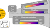 |
Fig. 1 Sketch of the model including all free model parameters. The free model parameters are further explained in Table 2. |
2 Method
2.1 The model
The model superimposes the flux of five distinct components to derive a total flux. These components represent the star, the optically thick inner rim of the disk, the optically thick dust mid-plane, the optically thin dust layer, and the molecular emission layer. The first four components are based on dust models by Juhász et al. (2009, 2010) while the molecular emission is computed using ProDiMo slab models (Arabhavi et al. 2024). The different components are visualized in Fig. 1.
The flux of the star ( ) is determined either through a stellar spectrum or a black body (ℬv) with a given temperature Tstar using the object’s distance (d) and the stellar radius Rstar:
 (1)
(1)
Another black body with a temperature Trim and its effective surface area Arim represents the flux ( ) arising from the inner rim of the disk:
 (2)
(2)
This component characterizes the hot, optically thick dust emission typically originating from the inner rim of a protoplanetary disk. The scaling factor (Crim) as for all continuum components, is introduced because of its use during the fitting procedure (Sect. 2.2).
The midplane component describes the optically thick dust emission originating at the disk layer where the optical depth is 1. We describe the bulk of this component by black bodies integrated from the inner ( ) to the outer radius (
 ) of this disk component:
 (3)
(3)
The inclination of the disk is noted as i. We note that the inclination of a model is treated as a simple scaling factor of the observed area and does not account for effects like occultations and different ray paths. A radial temperature power law with the exponent qmid is assumed as the midplane temperature profile (Tmid),
 (4)
(4)
with ( ) being the midplane temperature at the inner radius. Translating the integral in Eq. (3) into temperature space using Eq. (4) results in
 (5)
(5)
where the scaling factor Cmid incorporates all variables outside the integral and  describes the midplane temperature at
  . The derivation of Eq. (5) is shown in Appendix A.
The total emission of the optically thin dust is described by the component that we call the surface layer. Analogous to the midplane, we define the optically thin surface dust emission in our model as the radial integral of emission from  to
to  , with the additional factor of the cross section (
 ) of every dust species (j) multiplied by the dust column number density
  :
:
 (6)
(6)
We assume radius-independent column densities for all dust species with the same radial temperature power law (analogous to Eq. (4)) with an exponent qsur.  and
and  denote the temperature at the inner and outer radius, respectively. Therefore, Eq. (6) can be transformed to
 (7)
(7)
The factors outside the integral, excluding the opacity, are summarised as 
For the opacities of the optically thin dust component we assume single sized, homogeneous particles. For each dust material we pre-compute the opacities for a fixed number of particle sizes and treat each material and each particle size as a separate, independent dust component. The opacities are computed using the DHS method (Min et al. 2005) with the irregularity parameter fmax = 0.8, simulating irregularly shaped grains. The refractive index as a function of wavelength is taken from laboratory measurements (see Table 1).
The cumulative flux of the stellar, rim, midplane, and surface components has been demonstrated to sufficiently explain the mid-infrared flux of protoplanetary disks as observed by Spitzer (Juhász et al. 2009, 2010).
Here we expand this dust model to encompass a gaseous component. The flux  of each molecule (mol) is described by an integral of specific intensities
  along the radius of the emitting region:
 (8)
(8)
The temperature distribution for each molecule is a radial temperature power law with an exponent of qemis (same value for all molecules), and the molecules emit within individual radial (from  to
to  ) and temperature ranges (from
  to
to  ):
):
 (9)
(9)
The column density of every molecule (Σmol(r)) is defined as another radial power law between the column density Σmax at  and the column density Σmin at
 (10)
(10)
where the exponent pmol is defined by Σtmax and Σtmin. The radial integral in Eq. (8) can be substituted into a temperature integral using Eqs. (9) and (10), with Cmol summarizing all factors outside the integral:
 (11)
(11)
This treatment allows each molecule to emit over a temperature and column density range instead of single temperature and column density slabs, granting the model more flexibility. The emission  of each molecule at a given temperature T and column density Σmol is estimated by linear interpolation in the pre-calculated grids of ProDiMo 0D slab models introduced in Arabhavi et al. (2024). These grids span from 25 to 1500 and from 1014 to 1024.5 cm−2, in steps of 25 K temperature and 1 /6 dex column density, respectively. The model spectra cover the MIRI wavelength range with a very high spectral resolution of R = 105 to account for line opacity overlap, which is important for molecules that are extremely optically thick. The resulting spectra are convolved with R = 3000. We note that for this particular project, the narrow fitted wavelength region of GW Lup justifies the use of a constant R. Changing R to 2500 does not significantly impact the retrieved parameter values. The level populations are calculated in local thermal equilibrium (LTE) and the line profiles are assumed to be Gaussian. The details of the slab models can be found in Arabhavi et al. (2024).
These grids exist for H2O (o-H2O/p-H2O = 3), CO2, HCN, HC3N, CH4, C2H2, C2H4, C2H6, C3H4 (only up to 600 K), C4H2, and C6H6 (only up to 600 K). The spectroscopic data and partition sums are largely taken from the HITRAN 2020 database (Gordon et al. 2022). For C3H4 and C6H6, the data are taken from Arabhavi et al. (2024). The LAMDA database (Schöier et al. 2005) is used for H2O1. Molecules for which the spectroscopic data of the isotopologues are available, isotopic abundance fractions of 70 and 35 are used for one and two carbon-bearing hydrocarbons respectively (Woods & Willacy 2009).
The total model flux (Fv) is given by the sum of the stellar, dust continuum, and molecular emission line contributions:
 (12)
(12)
An example of such a model is provided in Fig. 2. The individual components are visualized, with their summation making up the full model.
All free parameters describing the model are listed in Table 2 and visualized in Fig. 1. There are 14 free parameters plus 1 and 5 additional free parameters per dust species and molecule, respectively. We note that Crim and Cmid are proportional to the physical parameters of Arim and 
The abundance factor of each dust species  is proportional to their dust masses (Appendix B). By knowing the radial structure, the radius of the effective emission area (Reff) for an observer can be calculated using the inclination (i) and the inner (Rmin) and outer radius (Rmax) of the component:
 (13)
(13)
This radius is equivalent to the emitting radius that is fitted using slab models (e.g. Grant et al. 2023; Perotti et al. 2023).
The model can also be used without the gaseous component (DuCK: Dust Continuum Kit), making it a tool to examine dust compositions. Jang et al. (in prep.,) will present an analysis the dust composition of PDS 70 based on JWST/MIRI observations based on DuCK.
A single DuCKLinG model describing the dust and gas simultaneously typically takes no longer than a few milliseconds to run. Notably, this allows many molecules to be incorporated into a full Bayesian fitting procedure.
References for the laboratory data for the dust species.
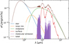 |
Fig. 2 Example model. The brown line shows the total flux of the model. This flux is a combination of stellar flux (blue), rim flux; (orange), midplane flux (green), surface flux (red), and molecular emis-sion (purple). |
Free parameters of the model.
2.2 Fitting procedure
We fitted the model to observations using MultiNest (Feroz & Hobson 2008; Feroz et al. 2009, 2019) through the Python package PyMultinest (Buchner et al. 2014) to retrieve values and uncertainties for our model parameters. This Bayesian inference tool determines the posterior distribution for all parameters using multimodal nested sampling. The details of the algorithm are given in the references above.
The quality of a model fit for a particular observation is quantified by a likelihood function ℒ that evaluates the differences between the model spectrum Fi,model and the observations Fi,obs with uncertainties σiı0bs, where i = 1… Nobs is an index running through a selected wavelength range:
 (14)
(14)
We treated the observational uncertainty as a free parameter to avoid the need to manually determine the uncertainty based on the noise of a line-free region. Assuming that the uncertainty is proportional to the flux of the observation, the parameter aobs defines σi,obs as
 (15)
(15)
The model flux Fi,model is calculated from Eq. (12) at the wavelength points of the observations, using the Python package SpectRes (Carnall 2017) to rebin the data. This package evaluates the fraction of every model wavelength bin that falls in each observational bin in a highly optimized way. Based on this, the fluxes corresponding to the new wavelength grid are calculated.
Likelihood calculations including the flux prediction of one model are done within milliseconds. Nevertheless, the determination of a posterior is computationally expensive due to the large number of parameters (see Table 2). A reduction of the number of parameters sampled with MultiNest is needed. This is typically done by fixing parameters to known values. The only parameters in our model with literature values are the stellar parameters, the inclination, and distance. Fixing them still leaves many free parameters (for a fit with 10 dust species and 5 molecules, 46 parameters are needed).
We decreased the parameter space further by exploiting the linearity of certain parameters. The scaling factors (Crim, Cmid), the abundances of the dust species ( ), and the scaling factor of every molecule (Cmol) are linear parameters. This means that they scale the respective model components without changing the shape of them. Therefore, we can use a simple non-negative least square solver (NNLS) by SciPy (Virtanen et al. 2020) to obtain the optimal values of the linear parameters for a given set of the non-linear parameters. This leads to the procedure outlined in Fig. 3. The likelihood of a model is calculated given its non-linear parameters. The linear parameters are calculated using NNLS, and all parameters are finally used to predict the model flux and calculate the corresponding likelihood. For the aforementioned example, this reduces the number of free parameters from 46 to 31 .
Our fast approach comes at the cost of a less accurate Bayesian sampling of the full parameter space. We examine the consequences of this approach in detail in Sect. 3.1, where we compare our results to those obtained using a full Bayesian sampling of all parameters.
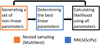 |
Fig. 3 Sketch of the fitting procedure. While the nested sampling algorithm (orange) creates all non-linear parameters, the linear parameters (two parameters plus one per dust species and one per molecule) are determined by non-negative least squares (NNLS; blue). The total set of parameters is then used to calculate the likelihood. |
3 Results
3.1 Validating the fitting procedures
We validated our procedures by fitting a DuCKLinG mock observation to check whether we can retrieve the chosen parameter values. We did this twice, first with the full Bayesian analysis for all parameters and then for the accelerated method described in Sect. 2.2. A mock observation is created using DuCKLinG with 5 dust species (all species listed in Table 1 with a size of 2 µm are included with identical scaling factors  ) and emission from H2O and CO2 (both with Reff = 0.1 au), with a spectral resolution of 3000, spanning the entire JWST/MIRI wavelength range, assuming a relative flux uncertainty of 0.1% for the unscattered mock observation.
For this exercise, we fixed most parameters to their true values, except for the exponents of the temperature power laws (qmid, qmid, and qemis), Crim, Cmid, the dust abundances, and the molecular parameters (18 parameters). The fast retrieval finds the linear parameters (Crim, Cmid, all abundances of the dust species, and the emitting radii of the molecules) with NNLS, and only uses MultiNest to determine the remaining 11 parameters. The priors of the fast approach are listed in Table 3. The prior ranges include the true values (qmid = –0.6, qsur = –0.55, and qemis = –0.55; CO2 emitting from 200K/1017 cm−2 to 500K/1021 cm−2, H2O emitting from 200K/1017cm−2 to 900K/1019cm−2). All prior ranges are chosen to be relatively narrow to increase the computational speed of the retrieval. The full approach uses additional priors for the Rmin (ℐ(10−3,100)) of both molecules and for all scaling factors (including dust abundances). Since the scaling factors can span orders of magnitude a trick is used to create narrower priors for these parameters. The scaling factor priors are defined with respect to the relative contribution (peak component flux to peak observed flux) of their components (ℐ(10−1,100)). A value of 10−1 corresponds to the parameter’s component having a peak flux that is 1% of the maximum observed flux. Since all components contribute significantly more than 1%, these priors incorporate the true values for Crim, Cmid, and all abundances of the dust species.
Figure 4 shows the mock observation compared to the median spectra from both posteriors. The retrieved spectra are shifted to allow for a visual comparison. As seen in the upper panel of Fig. 4, both retrieved spectra follow the overall shape of the mock observation well. The lower panel shows a zoom-in to the line-rich region around 6.5 µm, which gives an impression of the retrieved quality of the molecular emission. The mean differences between the posterior of spectra and the mock observation are 0.0017 and 0.0043% for the fast and full approach, respectively (see lower panel of Fig. 4). This is well below the observational uncertainty of 0.1%. Therefore, we conclude that both fitting approaches converge towards the optimal solution, with the fast approach resulting in slightly better model spectra. We comment on this when discussing the retrieved parameters.
Figure 5 shows the posteriors for all parameters derived with the two methods. The horizontal axes show the differences between the denoted parameters and the values that were used to create the mock observation. The vertical axis displays the number of posterior models within the parameter bins. The posterior distributions peak for both approaches at the values used to create the mock observation (x-value of 0 in all histograms of Fig. 5). While the histograms for both approaches match perfectly for most parameters, the dust abundances show some differences. Both posteriors peak around the true value, but the fast approach consistently finds smaller uncertainties for the dust abundances. Therefore, the fast approach has an unjustified confidence in the retrieved values for these specific parameters but overall retrieved the same values. This overconfidence can be explained by an unresolved degeneracy between the abundance of Mg-olivine and Mg-pyroxene. While the fast approach is solving for these parameters with NNLS and therefore jumping to the optimal solution all the time, the full approach explores these parameters in a Bayesian way and thus accounts for the non-optimal solutions that make up the degeneracy. This also explains the slightly better fitting quality of the fast approach. However, this non-resolving of degeneracies is not seen between non-linear parameters and the other linear parameters (1og Rmin for CO2, 1ogRmin for H2O, Crim and Cmid). These are resolved well with the fast method, which can be seen by the similar posterior width for all parameters except the dust species. Therefore, we conclude that the fast approach is a good representation of a full Bayesian approach, with only the uncertainties of specific parameters varying and the parameters of interest, the molecular parameters, basically unaffected.
This slightly lower accuracy comes with a huge benefit in computational speed. The full retrieval method needed about 165 mi11ion evaluations of the likelihood function to converge (defined by a log-evidence tolerance of 0.5); the fast retrieval method only needed about 530000 evaluations. Determining the linear parameters with NNLS increases the time for calculating the likelihood only by about 8%. The full approach can calculate slightly more models in parallel because fewer of them are accepted and used for the next iteration of the Bayesian analysis. Even accounting for all these factors, the fast retrieval method is faster by a factor of about 80 in wall time (fast retrieval time: ~15 min, full retrieval time: ~33 h). Therefore, the full approach is only feasible for problems with many fixed parameters (like the case presented here for validation), while the fast approach is the only practical option when fitting observational data with a handful of molecules.
Prior distributions of free parameters used for the comparison of the fast and full fitting approach.
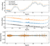 |
Fig. 4 Comparison of the mock observations and the spectra from the two retrieval approaches. The mock observation is shown in black. The median spectrum from the posterior derived using the fast and full approach are shown in orange (shifted up by 1 Jy) and blue (shifted up by 0.5 Jy), respectively. While the upper panel shows the full wavelength range of the mock observation, the middle panel shows a zoom-in to the line-rich region around 6.5µm. The lower panel displays the residual (defined as ((Fobs – Fmode1)/Fobs) in percent between the two retrievals and the mock observation, with the coloured areas indicating the 1σ uncertainty of the retrieved fluxes. |
3.2 Interpretation of the retrieved parameters
While our 1D model is physically more complete compared to 0D slab models that fit every molecule individually, one after the other, they are still much simpler than complex thermo-chemical disk models, such as ProDiMo (Woitke et al. 2009a), which determine the 2D chemical abundances of all species and the gas temperature structure in the disk consistently. A detailed fit of a 2D ProDiMo thermo-chemical disk model to a MIRI spectrum is computationally very challenging due to the high computational costs of about 50 CPU-hours per disk model. Woitke et al. (2024) have recently published such a fit for the case of EX Lup, which is the first and so far the only case where such a fit has been presented. To achieve this computational challenge, compromises regarding the fitting procedure compared to Bayesian analysis had to be accepted. On the other hand, complex 2D disk models can play an important role in interpreting MIRI data without the need to fit them to the spectra. They can (i) check if the conditions retrieved by simpler models are possible when accounting for the physics and chemistry in disks and in which environments they arise and (ii) they can analyse the effects of disk processes (e.g. dust evolution) and disk structures (e.g. gaps, inner cavities, rounded rims) on the observable spectra (e.g. Anderson et al. 2021; Greenwood et al. 2019; Vlasblom et al. 2024). Additionally, these complex models can benchmark simpler models and check how the retrieved parameters can be interpreted (Kamp et al. 2023).
In this section, we test the physical consistency of our retrieval results by fitting the mid-IR spectrum generated by a ProDiMo disk model for AA Tau. We focus on a comparison of the results describing the radial extension and physical conditions in the regions responsible for the H2O line emission.
The ProDiMo mock observation is created for the MIRI wavelength range with R = 3000. The spectrum includes H2O as the only molecule. For a detailed description of the underlying ProDiMo model (see Woitke et al. 2019; Kamp et al. 2023).
In our retrieval model, the stellar parameters, the disk inclination, and the distance are fixed to the values used in the mock ProDiMo model for AATau (Woitke et al. 2019): Tstar = 4160K, Rstar = 1.6813 R⊙, i = 59°, and d = 137.2 pc. The dust in our retrieval model is assumed to be composed of pure grains made of am Mg-olivine, am Mg-pyroxene, silica, forsterite, or enstatite, with all sizes being 0.1, 1.5,1.0, and 5.0 µm (as introduced in Table 1). The remaining free and non-linear parameters are listed with their prior distributions in Table 4. The prior ranges of the water parameters are based on the extent of the underlying slab model grid (see Sect. 2.1). The temperature priors of the dust components are chosen to incorporate the full posterior without parameters converging towards the edges of their prior range. We chose the priors of the temperature power law exponents to include known literature values from radial CO temperature profiles (–0.95 to –0.5, Fedele et al. 2016) and typical temperature slopes extracted from a thermo-chemical Herbig disk model (–0.6 and –0.4, Brittain et al. 2023).
Figure 6 shows that the retrieved shape of the dust features and the strengths of most water lines are reproduced well. The small deviation in the dust features (as seen in the residual in the lower panel of Fig. 6) are caused by the different dust properties used in the retrieval (Table 1) and the ProDiMo mock observation. While the 1 < deviation between model and observation (1.5mJy/0.61%) is slightly larger than the average noise (1 σ = 1 .5 mJy) that was used to create the mock observation, more than 99% of model fluxes are closer than 8 mJy/1.71% to the observation. There is no large systematic deviation between model and observation (mean residual is less 0.0011 mJy). In total, we conclude that the mock observation is well-fitted by our model.
To compare the properties of the line emitting regions between the ProDiMo model and our retrieval model, we must carefully define and extract these properties from the complex 2D ProDiMo disk structure. The line emitting conditions in ProDiMo are extracted from the regions where most of the line flux originates. Figure 7 illustrates this process. The radially and vertically cumulative fluxes of one specific line are used to determine the radial and vertical ranges where the central 70% of line emission (from R0.15. to R0.85 and from z0.15(r) to z0.85(r) originate, respectively. This region is called the line’s emitting region in ProDiMo. We define the emission temperature at every radius  as the vertical mean value of the gas temperatures that we find in the line emitting region. Concerning the molecular column densities, we define
  as the molecular column density over the height marked with τ = 1 in Fig. 7, where the vertical continuum optical depth at line centre wavelength approaches one. The column density hence depends not only on radius but also on the considered line, because the continuum optical depth depends on wavelength.
The line emitting conditions of a molecule in DuCKLinG are extracted in a similar fashion for comparability. The radially cumulative flux of H20 determines the inner (R0.15) and outer radius (R0.85) of region of significant emission (enclosing the central 70% of emission). Using Eqs. (9) and (10) the corresponding column densities (Σ0.15.is and Σ0.85) and temperatures (T0.15 and T0.15) at R0.15 and R0.85 are determined. Due to the similar extraction procedure, it is expected that the extracted quantities from ProDiMo and DuCKLinG overlap if the molecular emission in both models originates under similar conditions. Additionally, these extracted quantities from DuCKLinG are better indications of the emitting conditions of a molecule than Rmin/Rmax, Tmax/Tmin, and Σmax/Σmin. This can be seen in the example presented in Sect. 3.1. The upper right panel in Fig. 5 shows how the retrieved posteriors of Σmin for CÒ2 peaks at the true value of the mock observation, but is asymmetric with a larger extension towards smaller values. This means that extending the column density power law to lower values results in similar molecular fluxes. This is underlined by the slight asymmetry of Tmin and by a similar behaviour of water in Fig. 5. Therefore, the lowest temperature and column density can be misleading because the emission under these conditions does not contribute significantly to the overall flux.
The emission conditions of ProDiMo and the retrieved conditions by DuCKLinG are compared in Fig. 8. For ProDiMo we show  as a function of radius (grey lines) in Fig. 8, using all water lines with peak line strength above the noise of the mock observation. Additionally, the column densities at R0.15 to R0.85 are indicated with a circle that displays the vertical mean gas temperatures at these radii colour-coded. The retrieval results are visualised by a thick slanted bar, showing the retrieved power-law distribution of the column density as function of radius. The colour along that bar represents the retrieved emission temperatures. We note that the uncertainties of the endpoints of these power laws are smaller than the displayed line width.
In the ProDiMo model, the mid-infrared water lines are emitted from the surface of the disk close to the inner rim (inner part of region 3 in Fig. 1 of Woitke et al. 2009b). The water is created by two neutral-neutral reactions,
 (16)
(16)
followed by
 (17)
(17)
which have activation energies of 3150 and 1740 K, respectively (McElroy et al. 2013). Water is destroyed by photo-dissociation. Very close to the inner rim, stellar UV photons and X-rays penetrate the disk radially, which inhibits water formation. Once the radial column densities are large enough to shield the direct irradiation, the water concentration reaches its maximum value of about 10−4. Vertical integration down to the height where the dust becomes optically thick results in an about constant H2O column density as function of radius in the selected disk setup. The water line emitting disk surface ends quite abruptly where the gas temperature drops below about 200 K and the neutral-neutral reactions become inefficient.
The radial behaviour of temperature and column density overlaps well between ProDiMo and DuCKLinG from about 0.2 au outwards. Few water lines emit significantly further out (outermost emission from 6.6 au) or closer to the star (innermost emission from 0.1 au) in ProDiMo. The column densities retrieved by DuCKLinG fall also within the range of column densities of H2O in the ProDiMo model. The column densities for H2O in ProDiMo range from 4 × 1017 cm−2 to 5 × 1020 cm−2, which is larger than the range retrieved by DuCKLinG (3 × 1018 cm−2 to 3 × 1020 cm−2). The innermost very hot region (up to 1000 K) of water emission in ProDiMo is not reproduced by DuCKLinG (ranging only from about 200 to 400 K). Analysing the cumulative integrated line flux (upper panel of Fig. 8), we find that the hot inner region ( ) has an integrated line flux less than 3% of the total flux (2.3 × 10⁻¹⁷W/m2 to 8.8 × 10⁻¹⁶ W/m2). While weak lines can provide crucial information about conditions and processes in disks (e.g. Banzatti et al. 2023a), an automated fit of the full wavelength range naturally focuses on the strongest lines. For analysing weak lines in detail, a more focused approach is needed. Overall, there is good agreement between the emitting conditions in ProDiMo and the retrieved values from DuCKLinG. This makes us confident that the retrieved values by DuCKLinG are meaningful when fitting MIRI spectra.
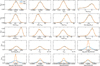 |
Fig. 5 Histograms of the posterior of all parameters for fits of the mock observations. The results obtained by fitting all parameters with MultiNest (full) are shown with blue lines. The results obtained with the accelerated method (fast) are shown with orange lines. The horizontal axis shows the parameter differences to the values used to create the mock observation. The vertical axis displays the fraction (fpost) of posterior models in the displayed bins. |
Prior distributions of free parameters used for the retrieval of the ProDiMo mock spectrum of AA Tau.
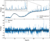 |
Fig. 6 Comparing the ProDiMo spectrum to the posterior of DuCK-LinG models. Upper panel: posterior distribution of the fit of a ProDiMo mock spectrum. The black line is the ProDiMo spectrum. The blue line shows the median fluxes from the models of the posterior distribution. The zoom-in on the upper left shows an enlarged version of the wavelength region from 22 to 24 µm. Lower panel: residual between the model fluxes and the ProDiMo spectrum. The blue line shows the median residual of all posterior models. The black area denotes the noise that was used to create the mock spectrum. |
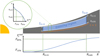 |
Fig. 7 Sketch of the line emitting region in a ProDiMo disk model. The cumulative line flux as function of radius is shown in the lower part, and the cumulative line intensity at some given radius, as function of height, is sketched in the insert on the top left. We consider the region between R0.15 and R0.85 and between z0.15(r) and z0.85(r) as the line emitting region, where the respective cumulative quantities reach 15 and 85%, respectively, Σ0.15 and Σ0.85 are the column densities at R0.15 and R0.85 respectively. |
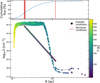 |
Fig. 8 Comparison of the radii, column densities, and line emission temperatures of H2O extracted from ProDiMo with the retrieved parameter conditions. In the main panel, the horizontal axis shows the radius of the emission and the vertical axis the column density. Every H2O line with peak fluxes 3σ above the observational noise is selected to show the emitting conditions in ProDiMo. The grey lines show |


3.3 Application to GW Lup
We fitted the JWST/MIRI spectrum of GW Lup using DuCKLinG to determine the continuum and molecular emission properties, including their uncertainties. This spectrum was published and fitted previously by Grant et al. (2023), using a continuum subtraction by hand followed by a sequence of χ2-fitting of OD slab models for single molecules as explained below. We compared these published results to the results that we obtained from our simultaneous Bayesian fit of all molecules and the continuum.
GW Lup is an M 1.5 star (Alcalá et al. 2017) at a distance of 155 pc (Gaia Collaboration 2020). The DSHARP survey (Andrews et al. 2018) found that the continuum emission shows a narrow ring at a radius of 85 au (Dullemond et al. 2018). Spectra with the Spitzer Space Telescope revealed emission of C2H2 (Banzatti et al. 2020) and strong emission of 12CO2 but no water (Pontoppidan et al. 2010; Salyk et al. 2011).
Grant et al. (2023) fitted the JWST/MIRI spectrum of GW Lup between 13.6 and 16.3 µm and detected in addition to the with Spitzer detected molecules 13CO2 for the first time, and H2O, HCN, and OH for the first time in this object. The fit to the MIRI-spectrum was obtained by Grant et al. (2023) by a step-by-step approach. First, the continuum was subtracted from the spectrum selecting 8 points of the spectrum by hand that likely show no line emission and a cubic spline interpolation. Then, the molecular emissions were fitted one by one, and subtracted, using the following sequence: H2O, HCN, C2H2, 12CO2, 13CO2, and OH. The emission spectrum of every single molecule was fitted using 0D slab-models of temperature T, column density Σcol, and the radius of a circular emitting area R. The fit of every molecular emission spectrum was obtained by χ2 minimisation using a grid of slab models.
We fitted the MIRI-spectrum between 13.6 and 16.3 µm with DuCKLinG. While this wavelength range encompasses no strong dust features and makes the determination of the dust composition difficult (see Appendix C), it enables comparison of the retrieved molecular properties to those from Grant et al. (2023). The stellar temperature (3630 K, Alcalá et al. 2017; Andrews et al. 2018), distance (155 pc, Gaia Collaboration 2020), and inclination (39°, Andrews et al. 2018) were fixed to their respective literature values during our fitting. The stellar radius (1.45 R⊙) was calculated using the Stefan-Boltzmann law with given stellar temperature and luminosity (0.33 L⊙, Alcalá et al. 2017; Andrews et al. 2018).
Our fit includes H2O, CO2,13 CO2, HCN, and C2H2. The column density ratio of 13CO2:12CO2 is fixed to 1:70. A ratio that falls within the allowable range for GW Lup derived by Grant et al. (2023). Therefore, only the values for CO2 are reported, which determine the 12CO2 and 13CO2 values. Contrary to Grant et al. (2023), we did not include OH in our analysis since non-LTE effects might play a significant role for this species. This decision does not significantly impact the remaining species, because Grant et al. (2023) found only weak OH features that do not overlap with the strongest features of the other species. The free parameters and their prior distributions are listed in Table 5 (the prior ranges are motivated in Sect. 3.2). We note that this table only includes the non-linear parameters. Additional linear parameters next to the midplane and rim scaling factors are the emitting radii of every molecule and the abundances of the different dust species. The linear parameters are automatically determined (see Sect. 2.2). The dust available during the fitting are am Mg-olivine, am Mg-pyroxene, silica, forsterite, and enstatite, all with sizes of 0.1, 1.5, 2.0, and 5.0 µm as introduced in Table 1.
The model spectrum extracted from the posterior distribution of the parameters is shown in the upper panel of Fig. 9. The black line shows the MIRI spectrum of GW Lup in the fitted wavelength range. The median flux of the posterior of models is shown in blue. The 1σ, 2σ, and 3σ level of the fluxes are shown in decreasing intensities of blue. There is large overlap between the model fluxes and the observation. Additionally, the spread of model spectra is very small, which means that the Bayesian algorithm is converging to a narrow solution. We extract one representative model from the posterior distribution to examine the fit composition in more detail. This median probability model is the model for which all parameters are closest to their posterior median as outlined by Kaeufer et al. (2023). While this model is not necessarily the model with the maximum likelihood, it is the closest to the median posterior values.
The different molecular contributions in this model are shown in the lower panel of Fig. 9. The 1σ difference between our model and the observations is 1.21 mJy or 0.64%. This is comparable to the retrieved observational uncertainty of 0.72%. All main spectral features are well reproduced: the CO2 feature at about 15 µm, the HCN feature around 14 µm, the C2H2 feature at about 13.7 µm, and all water lines at wavelengths longer than 15.5 µm. The few molecular lines that are present in the observation but not in the model (e.g. at about 15.2 or 16.1 µm) hint to contributions of molecules that were not included in our model or lines of included molecules that are not included in the used data collection. The slab-models by Grant et al. (2023) did not reproduce these lines as well, but focused their fits on narrow wavelength windows around the respective molecular features. If non-described emission becomes a substantial problem, it is possible with DuCKLinG to omit the respective wavelength ranges and derive a fit for the wavelength ranges that the model can describe.
Our retrieved molecular properties with their posterior uncertainties are listed in Table 6 together with the corresponding values derived by Grant et al. (2023). The retrieved dust composition is discussed in Appendix C. However, we note that the small wavelength range of the fit does not include any strong dust features, and therefore the retrieved dust composition should be taken with caution.
Our posterior distributions of the retrieved molecular column densities and emission temperatures are furthermore visualised in Fig. 10, keeping in mind that we use power laws for these quantities as function of radius for every molecule. The shaded areas colour-code how many of the posterior models emit at these conditions (between T0.15 and T0.85 as introduced in Sect. 3.2).
The column density ranges from our fit always include the values derived by Grant et al. (2023), at least within the 1σ ranges of its limits (Fig. 10). The temperature ranges for H2O and CO2 include the temperature values found by Grant et al. (2023). Interestingly, the water emissions in our model seem to originate from varying power laws that intersect at a point close to the value of Grant et al. (2023; see Fig. 10). Therefore, the water emission from this area seems to be of great importance to reproduce the observed features.
For C2H2, the previously found value of 500 K falls within the 1 σ -uncertainty of the lower T-limit found by this study (540 K), but our models also suggest contributions from significantly higher temperatures. Figure 10 shows how our posterior emitting conditions for C2H2 overlap with the best fit value derived by Grant et al. (2023).
For HCN, the previously found value (875 K) is significantly higher than the upper limit of our retrieved temperature interval up to 750 K, even including the 1e uncertainty of this limit. This can also be seen in Fig. 10, where the value from Grant et al. (2023) falls outside of the posterior distribution of the emission properties for HCN. This difference might originate from our use of temperature and column density ranges, the different treatment of the continuum, or the fitting procedure in both studies. In Sect. 4 we show that the change from single values to ranges for the temperature and column density is not responsible for the retrieved differences and elaborate further on the potential reasons.
Comparing the emitting areas, we find that the values retrieved in our study are slightly smaller than the values found by Grant et al. (2023; except for CO2, which has identical values in both approaches). Due to our inclusion of an inclination, we expect the values for Reff to be slightly larger (factor of (cos 39°)-1/2 ≅ 1.13) than the ones found by Grant et al. (2023). We explain this by the column density ranges that generally reach higher densities in our model than the single values, which in turn requires a smaller emitting area to reproduce the same flux. This can be tested by calculating the total number of molecules contributing to the total flux per molecule. The total number of molecules  is calculated as the integral of column densities Σmol over the annuii from the inner (R0.15) to the outer (R0.15) radius with significant emission:
 (18)
(18)
These total numbers of molecules are compared at the end of Table 6. We expect, similarly to the radius, that the values of this study are increased by a small factor ((cos39º)−1 ≃ 1.29) compared to the previously derived results. The values from Grant et al. (2023) fall within or close to the 1σ uncertainties for H20 and HCN. C2H2 has the largest uncertainty. We show in Sect. 4 that the simultaneous fitting of all molecules enables us to account for the contributions of other molecules at the wavelength range of the C2H2 feature. This decreases the amount of C2H2 needed to reproduce the spectrum.
The differences for CO2 can be explained by the different treatment of 13CO2 in our modelling approach. To allow for line overlap between isopologues, we fixed the ratio of 13CO2 to 12CO2 to 1:70, while Grant et al. (2023) treats them as independent species, allowing for other ratios and differences in temperature. However, Grant et al. (2023) finds the literature value of the ratio to be within the allowed range and the retrieved temperature of 13CO2 is only 75 K lower than the temperature of 12CO2. This is smaller than the temperature range retrieved by DuCKLinG and on a similar scale as the temperature error bars on the higher temperature limit. This makes us confident that constraining the fit to a fixed 13CO2 to 12CO2 ratio is justified by the benefit of line overlap. The total number of 13CO2 molecules we retrieved is  , which is close to the value of 9.3(+4l) found by Grant et al. (2023). Therefore, our slightly larger total number of 12CO2molecules is needed to produce a similarly strong 13CO2 feature.
While there is a large overlap between the molecular properties retrieved by us in this study and by Grant et al. (2023), we note that the advantage of our method is (i) the inclusion of an automated fitting of the continuum and (ii) the simultaneous Bayesian fitting of all parameters. It seems that for this particular object, the manual continuum subtraction by Grant et al. (2023) worked quite well. However, this procedure becomes more challenging when optically thick molecular line emission creates a quasi-continuum (Tabone et al. 2023). Additionally, the considerable difference (e.g. total number of C2H2 molecules) might be due to propagating errors with the iterating molecular fitting process. The Bayesian fitting of all molecules does circumvent this, especially if the molecular features are overlapping.
Besides the retrieval of the molecular emission properties, we simultaneously extract some dust properties with our fitting routine (see upper half of Table 6). The temperature parameters (especially the maximum temperatures) are poorly constrained due to the small wavelength range (13.6–16.3 µm) of the fitted observation. Therefore, the provided uncertainties are dominated by the provided priors. The power law exponent of the gas emission (qemis) is relatively well constrained and falls within the poorly constrained range of the dust surface layer exponent (qsur). Similar values might hint towards a common layer, located at similar heights over the disk midplane, from which both the optically thin dust emission and the molecular emission lines are emitted.
The last non-molecular parameter listed in Table 6 is aobs, and it denotes the observational uncertainty relative to the observed flux (see Eq. (15)). The retrieved uncertainty of 0.723% results in an average σobs of 1.43 mJy, which is larger than the value of 0.44 mJy determined by Grant et al. (2023) based on the noise of a line free region from 15.9 to 15.94 µm. We note that the retrieved a0bs is not model-independent, since it denotes the uncertainty that best explains the differences between model and observation. Therefore, it can be seen as an upper estimate for the observational uncertainty of the fitted spectrum, which makes it consistent with the previously determined value.
Prior parameter ranges for fitting the GW Lup’s MIRI spectrum.
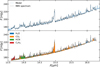 |
Fig. 9 Comparing the MIRI spectrum of GW Lup to the retrieved DuCKLinG models. Upper panel: spectral posterior distribution for a fit of the GW Lup MIRI spectrum. The black line represents the MIRI spectrum. The blue line shows the median fluxes from the models of the posterior distribution. The blue lines consist of contours that represent the 1σ, 2σ and 3σ level of the fluxes. Lower panel: median probability model. The black line represents the MIRI spectrum. The lower edge of the coloured region shows the continuum emission of the model, with the cumulative molecular emission shown in different colours. |
Posterior parameter values and uncertainties for selected parameters of the GW Lup fit.
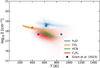 |
Fig. 10 Molecular emission properties of GW Lup. The different coloured areas denote the parameter areas in which the respective molecule is significantly (as introduced in Sect. 3.2) emitting in the posterior of models. The points show the retrieved parameter values by Grant et al. (2023) for the same molecules. |
Bayes factors of different fits of GW Lup.
4 Discussion
Our Bayesian analysis allowed us to quantify the benefits of using simple or more complex models. In the DuCKLinG models, the molecules are allowed to emit from radial ranges of column densities and emission temperatures, but we can also enforce single values of these quantities. In the most simplified case, the model falls back to simultaneous 0D slab-model fits on top of the dust continuum.
Table 7 compares different models of reduced complexity, in application to the GW Lup spectrum, to the full model as discussed in Sect. 3.3. The comparison is done using the Bayes factor (B), which compares the evidence (p(d\M1\)) of the observed data (d) for one model Mı to the evidence (p(d\M2)) for another model M2 :
 (19)
(19)
We note that ln B < 1, 1 < ln B < 2.5, 2.5 < ln B < 5, 5 < ln B < 11, and 11 < ln B correspond to no evidence, weak evidence, moderate evidence, strong evidence, and very strong evidence, respectively, for a variant model (M1) over the full model (M2 ) (Trotta 2008). The sign of B indicates which model is preferred, with negative values meaning that the full model is preferred.
Table 7 lists these Bayes factors for altogether 9 models, using either a single column density value or single values for both the column density and the emission temperature, for one selected molecule as indicated. All other molecules are still fitted using ranges for both column densities and emission temperatures. Additionally, one model labelled with ‘all’ uses 0D slab-models (single values for column density and temperature) for all molecules.
We found no evidence that varying column densities and emission temperatures are required to fit the observations of HCN and C2H2 for the case of GW Lup, which hints that the emission regions for these molecules do probably not show a large diversity in conditions. For CO2 there is weak evidence that a column density range is needed (ln B = –1.61) and very strong evidence against a single column density and temperature description (ln B = –21.55). Therefore, it seems that CO2 is emitted from a region that varies in column density and temperature. Similarly, we find weak evidence (ln B = –2.42) that varying emission temperatures are required for H2O, given the observations.
For the model that used 0D slab models for all molecules, there is very strong evidence (logarithm of the Bayes factor of 23.16) that it cannot reproduce the observations as well as our full model. This is largely driven by the worse fitting of H2O and CO2 by the 0D slabs, since the Bayes factors for the reduced model of only HCN and C2H2 are not significant.
However, this model allows for a comparison to the fitting results from Grant et al. (2023) with identical complexities for the molecular emission. Fig. 11 shows the emission conditions retrieved by the model using 0D slabs for all molecules. The shared areas result from the variation of temperature and column density in the posterior of models.
For both water (temperature:  column density:
  and CO2 (temperature:
  ; column density:
  the posterior is well constrained to values close to the ones extracted by Grant et al. (2023; see Table 6 for the values). This supports the interpretation that the observed water features require emission conditions close to the values from Grant et al. (2023).
The conditions of C2H2 are rather poorly constrained with the temperature  having error bars larger than 100 K and the column density having a lower 1er limit of 3.3(+15) cm–2 nearly two orders of magnitudes lower than the median value 1.5(+17)cm–2. The large uncertainty in column density is most likely due to the gas being optically thin, which makes the emitting area and column density completely degenerate. This degeneracy of C2H2 is also found by Grant et al. (2023).
Most striking are the retrieved differences for HCN. While the column density retrieved by Grant et al. (2023) falls within the by DuCKLinG retrieved range  , the temperature of 875 K shows large disagreement
  . A similar difference is seen in the full retrieval (Sect. 3.3). Therefore, we conclude that the difference is not due to the different treatment of the continuum and fitting procedure instead of the used model complexity. It can be seen that the HCN feature at about 14 µm (Fig. 9) shows a non-negligible flux from CO2 over the full wavelength range as well. While the Bayesian analysis employed in this study optimises the CO2 and HCN conditions at the same time, the iterative fitting procedure by Grant et al. (2023) fits HCN before subtracting the flux from CO2. Therefore, we speculate that the iterative fitting is the origin of the discrepancy in retrieved temperatures for HCN between this study and Grant et al. (2023). This underlines the need for Bayesian analysis with a model that describes the molecular emission by all molecules and the dust emission at the same time to interpret JWST/MIRI spectra.
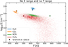 |
Fig. 11 Molecular emission properties of GW Lup for the 0D slab retrieval. The different coloured areas denote the parameter area under which the respective molecule is emitting in the posterior of models. The points show the retrieved parameter values by Grant et al. (2023) for the same molecules. |
5 Summary and conclusion
In this paper, we have introduced DuCKLinG, a Python-based computer code that can be used to simultaneously model the dust continuum and molecular emission properties of protoplanetary disks. The model is a superposition of optically thick and thin dust emission based on the dust models by Juhász et al. (2009, 2010) and slab models describing the molecular emissions from a handful of molecules in LTE. While previous studies used single values for column density and emission temperature for each molecule, we allowed the radial power-law distributions of column densities and emission temperatures for each molecule to describe the spectra observed with JWST/MIRI. The model is very flexible and applicable in many cases (e.g. different stellar types, disk structures, and inclinations). Possible limitations are the exclusion of non-LTE effects, which have been shown by Banzatti et al. (2023b) to be relevant for water, especially at short wavelengths (<9 µm), and the lack of absorption lines due to the independent treatment of dust and gas. This might be worth exploring in future projects. Our model spectra can be compared to observations employing a full Bayesian analysis since the code is speed optimized and requires only about 6 CPU milliseconds to generate one model spectrum. Among other things, this allows for an automated analysis of large samples and analysis of the preference of different complexities (e.g. which molecules are emitting under diverse or homogeneous conditions). The main conclusions of this paper are as follows:
Determining linear parameters with NNLS instead of Bayesian sampling decreases the computational time of the retrieval by a factor of about 80 for a mock observation and does not significantly change the retrieved median posterior values.
The model can reproduce a mock observation by ProDiMo with a lee deviation of only 2.5 mJy. The retrieved emission conditions describing the H2O emission correspond well with emitting conditions in complex thermo-chemical codes such as ProDiMo.
The model can successfully reproduce the MIRI spectrum of GW Lup without the need for a continuum subtraction.
The retrieved molecular conditions for GW Lup overlap well with values extracted from slab models by Grant et al. (2023). Temperature differences for HCN are attributed to the simultaneous fitting procedure compared to iterative fitting and not to the introduction of temperature and column density ranges.
We conclude that H2O and CO2 are emitting from a radially extended region of GW Lup that varies significantly in temperature but, at least for H2O, not in column density. The emission of HCN and C2H2 originates from a narrow region that does not show a large variety of emitting conditions (column density and temperature).
We show that it is possible to retrieve the optically thin dust composition at the example of GW Lup. However, we note that the selected wavelength range does not allow for reliable dust composition constraints and should be taken as motivation for future studies.
The strong overlap between this study and results obtained by Grant et al. (2023) show that fits based on continuum subtraction and slab models are a valid approach to analyse MIRI spectra. This might be more challenging however for observations with strongly overlapping dust and gas features. In this case, DuCKLinG can become an important tool to analyse the molecular emission and dust mineralogy in an automated way.
Acknowledgements
We acknowledge funding from the European Union H2020-MSCA-ITN-2019 under grant agreement no. 860470 (CHAMELEON).
Appendix A Derivation of model components
In this section, the integral substitution from Eq. (3) to Eq. (5) is shown. This is equivalent to the translations of Eq. (6) to Eq. (7) and Eq. (8) to Eq. (11). Using the temperature power law (Eq. 4) it follows that
 (A.1)
(A.1)
This means that,
 (A.2)
(A.2)
using the expression 2/qmid – 1 = (2 – qmid)/qmid· Therefore, r dr can be substituted in Eq. (3), which results in Eq. (5).
The surface layer uses the same relations with their component's respective quantities with the additional factor of  Analogously, Eq. (8) uses the molecular intensities instead of the black bodies of Eq. (3), but the derivation stays the same.
Appendix B Calculation of the dust mass
In this section, we derive the optically thin mass per dust species based on  . The total mass of a dust species Mj is given by
![Mathematical equation: $M = \pi \left[ {{{\left( {R_{\max }^{{\rm{sur}}}} \right)}^2} - {{\left( {R_{\min }^{{\rm{sur}}}} \right)}^2}} \right]{{\rm{\Sigma }}_j}$](/articles/aa/full_html/2024/07/aa49936-24/aa49936-24-eq128.png) (B.1)
(B.1)
using the assumption that the column density Σj is constant within the disk. Using the relation between temperature and radius,
 (B.2)
(B.2)
Eq. (B.1) can be translated to
![Mathematical equation: $M = \pi \left[ {{{\left( {R_{\min }^{{\rm{sur}}}} \right)}^2}\left( {{{\left( {{{T_{{\rm{sur}}}^{\min }} \over {T_{{\rm{sur}}}^{\max }}}} \right)}^{\left( {2/{q_{{\rm{sur}}}}} \right)}} - 1} \right)} \right]{{\rm{\Sigma }}_j}.$](/articles/aa/full_html/2024/07/aa49936-24/aa49936-24-eq130.png) (B.3)
(B.3)
The column number density  can be translated to the mass coloumn destiny using
 (B.4)
(B.4)
where mj is the mass per dust grain. Therefore, Eq. (B.3) translates; to
![Mathematical equation: $M = \pi \left[ {{{\left( {R_{\min }^{{\rm{sur}}}} \right)}^2}\left( {{{\left( {{{T_{{\rm{sur}}}^{\min }} \over {T_{{\rm{sur}}}^{\max }}}} \right)}^{\left( {2/{q_{{\rm{sur}})}}} \right.}} - 1} \right)} \right]N_d^j{m_j}.$](/articles/aa/full_html/2024/07/aa49936-24/aa49936-24-eq133.png) (B.5)
(B.5)
The inner radius of the surface layer and the column number density can be expressed by  as shown in Eq. (7). This results in
 (B.6)
(B.6)
which only contains variables that are determined during the fitting procedure.
Appendix C The dust composition of GW Lup
One advantage of DuCKLinG is the simultaneous fitting of dust and gas, which allows for conclusions about the dust mineralogy in protoplanetary disks. In this section, we examine the retrieved dust composition of GW Lup for the fit presented in Sect. 3.3. However, we note that the fitted wavelength region was selected to compare the molecular results to Grant et al. (2023) and not optimised to retrieve well-constrained dust properties. The limited wavelength region (2.7 µm) lacks clear dust features, which complicates the retrieval of the dust composition. Therefore, the results presented here should be taken as a motivation for the possible application of DuCKLinG and not as an attempt to get reliable dust constraints.
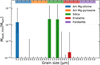 |
Fig. C.1 Histograms of the optically thin dust masses retrieved for GW Lup. The different dust species are colour-coded with the horizontal axis displaying the grain size. The histogram (dotted) displays the median absolute optically thin dust mass (Mdust,thin) of the respective species. It is accompanied by error bars that show the 1σ and −1σ-uncertainty. |
The optically thin dust mass for all dust species included in the retrieval is shown in Fig. C.1. A dust species is thereby defined as a material and a grain radius. Many dust species are not selected during the fitting procedure to reproduce the observation, which is an effect of the NNLS fitting. The NNLS solver determines the dust scaling factors and therefore the dust masses to best reproduce the observation. A dust mass of 0 M⊙ is thereby an option if the dust species does not improve the fit quality. Only four dust species are included in more than 25 % of the posterior models. These included species are Mg-olivine grains of size 0.1 µm, silica grains of size 0.1 µm and 2.0 µm and enstatite of size 1.5 µm. All other species seem to be unimportant to reproduce the observation from l3.6µm to 16.3µm.
Silica grains of sizes 0.1 µm and 2.0 µm have optically thin masses of 2.2 × 10⁻⁸ M0 with an upper 1er limit of 1.5 × 10⁻⁷ M⊙, and 2.1 × 10⁻⁸ M⊙ with an upper 1er limit of 1.7 × 10⁻⁷ M⊙, respectively. The olivine grains of size 0.1 µm have a mass of 1.4 × 10⁻⁸ M⊙. While the lower uncertainty of the dust masses for both silica grains is 0M⊙, the lower limit of olivine is 3.4 × 10⁻⁹ M⊙. Additionally, enstatite grains of size l.5µm are included in the models of the posterior with a median mass of 8.9 × 10⁻⁹ M⊙.
While Fig. C.1 shows the retrieved dust masses for all species, it does not provide information about which dust species are used at the same time. Some models of the posterior might use one combination, while others use a different one with a similar effect. Therefore, Fig. C.2 indicates which dust species are used together. Every row selects only the models of the posterior for which the dust species listed on the vertical axis was used in significant abundance (more than 10-12 M⊙). Focusing on these models the horizontal axis indicates the faction of models ( ƒmodel) that include the listed species simultaneously.
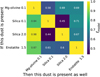 |
Fig. C.2 Heatmap showing which dust species and sizes are simultaneously used to describe the MIRI spectrum of GW Lup. The plot should be read row by row. One row indicates all models of the posterior that include the dust species named on the y-axis. The single entries show the faction of models (ƒmodel) that use the dust species on the x-axis at the same time. |
Focusing on the second and third rows, it becomes clear that the models including silica grain of size 0.1 µm and 2.0 µm only include the other silica size in 45% and 44% of the cases, respectively. This shows that these two grains are degenerate enough that the differences can be compensated by the remaining dust species. The left-most column of the heatmap shows that Mg-olivine of size 0.1 µm is used in the vast majority of all cases, no matter what other dust species is selected.
We note that the dust properties could be much better constrained when we had used the full MIRI wavelength range. Therefore, the results presented here should be taken as a motivation to try using DuCKLinG or DuCK (Dust Continuum Kit) to determine the dust mineralogy similar to Jang et al. (in prep).
References
- Alcalá, J. M., Manara, C. F., Natta, A., et al. 2017, A&A, 600, A20 [NASA ADS] [CrossRef] [EDP Sciences] [Google Scholar]
- Anderson, D. E., Blake, G. A., Cleeves, L. I., et al. 2021, ApJ, 909, 55 [NASA ADS] [CrossRef] [Google Scholar]
- Andrews, S. M., Huang, J., Pérez, L. M., et al. 2018, ApJ, 869, L41 [NASA ADS] [CrossRef] [Google Scholar]
- Arabhavi, A., Kamp, I., Henning, T., et al. 2024, Science, 384, 1086 [NASA ADS] [CrossRef] [Google Scholar]
- Banzatti, A., Pascucci, I., Bosman, A. D., et al. 2020, ApJ, 903, 124 [NASA ADS] [CrossRef] [Google Scholar]
- Banzatti, A., Pontoppidan, K. M., Carr, J. S., et al. 2023a, ApJ, 957, L22 [NASA ADS] [CrossRef] [Google Scholar]
- Banzatti, A., Pontoppidan, K. M., Pére Chávez, J., et al. 2023b, AJ, 165, 72 [CrossRef] [Google Scholar]
- Brittain, S. D., Kamp, I., Meeus, G., Oudmaijer, R. D., & Waters, L. B. F. M. 2023, Space Sci. Rev., 219, 7 [NASA ADS] [CrossRef] [Google Scholar]
- Buchner, Georgakakis, Nandra, et al. 2014, A&A, 564, A125 [NASA ADS] [CrossRef] [EDP Sciences] [Google Scholar]
- Carnall, A. C. 2017, arXiv e-prints [arXiv:1785.85165] [Google Scholar]
- Chiang, E. I., & Goldreich, P. 1997, ApJ, 490, 368 [Google Scholar]
- Dorschner, J., Begemann, B., Henning, T., Jaeger, C., & Mutschke, H. 1995, A&A, 300, 503 [Google Scholar]
- Dullemond, C. P., Dominik, C., & Natta, A. 2001, ApJ, 560, 957 [NASA ADS] [CrossRef] [Google Scholar]
- Dullemond, C. P., Birnstiel, T., Huang, J., et al. 2018, ApJ, 869, L46 [NASA ADS] [CrossRef] [Google Scholar]
- Fabian, D., Henning, T., Jäger, C., et al. 2001, A&A, 378, 228 [NASA ADS] [CrossRef] [EDP Sciences] [Google Scholar]
- Fedele, D., van Dishoeck, E. F., Kama, M., Bruderer, S., & Hogerheijde, M. R. 2016, A&A, 591, A95 [NASA ADS] [CrossRef] [EDP Sciences] [Google Scholar]
- Feroz, F., & Hobson, M. P. 2008, MNRAS, 384, 449 [NASA ADS] [CrossRef] [Google Scholar]
- Feroz, F., Hobson, M. P., & Bridges, M. 2009, MNRAS, 398, 1601 [NASA ADS] [CrossRef] [Google Scholar]
- Feroz, F., Hobson, M. P., Cameron, E., & Pettitt, A. N. 2019, Open J. Astrophys., 2, 10 [Google Scholar]
- Gaia Collaboration 2020, VizieR Online Data Catalog: I/350 [Google Scholar]
- Gasman, D., van Dishoeck, E. F., Grant, S. L., et al. 2023, A&A, 679, A117 [NASA ADS] [CrossRef] [EDP Sciences] [Google Scholar]
- Gordon, I. E., Rothman, L. S., Hargreaves, R. J., et al. 2022, J. Quant. Spec. Radiat. Transf., 277, 107949 [NASA ADS] [CrossRef] [Google Scholar]
- Grant, S. L., van Dishoeck, E. F., Tabone, B., et al. 2023, ApJ, 947, L6 [NASA ADS] [CrossRef] [Google Scholar]
- Greenwood, A. J., Kamp, I., Waters, L. B. F. M., Woitke, P., & Thi, W. F. 2019, A&A, 626, A6 [NASA ADS] [CrossRef] [EDP Sciences] [Google Scholar]
- Henning, T., & Mutschke, H. 1997, A&A, 327, 743 [NASA ADS] [Google Scholar]
- Jaeger, C., Molster, F. J., Dorschner, J., et al. 1998, A&A, 339, 904 [Google Scholar]
- Jäger, C., Dorschner, J., Mutschke, H., Posch, T., & Henning, T. 2003, A&A, 408, 193 [NASA ADS] [CrossRef] [EDP Sciences] [Google Scholar]
- Juhász, A., Henning, T., Bouwman, J., et al. 2009, ApJ, 695, 1024 [CrossRef] [Google Scholar]
- Juhász, A., Bouwman, J., Henning, T., et al. 2010, ApJ, 721, 431 [Google Scholar]
- Kaeufer, T., Woitke, P., Min, M., Kamp, I., & Pinte, C. 2023, A&A, 672, A30 [NASA ADS] [CrossRef] [EDP Sciences] [Google Scholar]
- Kamp, I., Henning, T., Arabhavi, A. M., et al. 2023, Faraday Discuss., 245, 112 [NASA ADS] [CrossRef] [Google Scholar]
- Khorshid, N., Min, M., Désert, J. M., Woitke, P., & Dominik, C. 2022, A&A, 667, A147 [NASA ADS] [CrossRef] [EDP Sciences] [Google Scholar]
- Liu, Y., Pascucci, I., & Henning, T. 2019, A&A, 623, A106 [NASA ADS] [CrossRef] [EDP Sciences] [Google Scholar]
- McElroy, D., Walsh, C., Markwick, A. J., et al. 2013, A&A, 550, A36 [NASA ADS] [CrossRef] [EDP Sciences] [Google Scholar]
- Min, M., Hovenier, J. W., & de Koter, A. 2005, A&A, 432, 909 [NASA ADS] [CrossRef] [EDP Sciences] [Google Scholar]
- Mollière, P., Molyarova, T., Bitsch, B., et al. 2022, ApJ, 934, 74 [CrossRef] [Google Scholar]
- Öberg, K. I., Murray-Clay, R., & Bergin, E. A. 2011, ApJ, 743, L16 [Google Scholar]
- Palik, E. D. 1985, Handbook of Optical Constants of Solids (Amsterdam: Elsevier) [Google Scholar]
- Perotti, G., Christiaens, V., Henning, T., et al. 2023, Nature, 620, 516 [NASA ADS] [CrossRef] [Google Scholar]
- Pontoppidan, K. M., Salyk, C., Blake, G. A., et al. 2010, ApJ, 720, 887 [CrossRef] [Google Scholar]
- Salyk, C., Pontoppidan, K. M., Blake, G. A., Najita, J. R., & Carr, J. S. 2011, ApJ, 731, 130 [Google Scholar]
- Schöier, F. L., van der Tak, F. F. S., van Dishoeck, E. F., & Black, J. H. 2005, A&A, 432, 369 [Google Scholar]
- Tabone, B., Bettoni, G., van Dishoeck, E. F., et al. 2023, Nat. Astron., 7, 805 [NASA ADS] [CrossRef] [Google Scholar]
- Trotta, R. 2008, Contemp. Phys., 49, 71 [Google Scholar]
- Virtanen, P., Gommers, R., Oliphant, T. E., et al. 2020, Nat. Methods, 17, 261 [Google Scholar]
- Vlasblom, M., van Dishoeck, E. F., Tabone, B., & Bruderer, S. 2024, A&A, 682, A91 [NASA ADS] [CrossRef] [EDP Sciences] [Google Scholar]
- Woitke, P., Kamp, I., & Thi, W. F. 2009a, A&A, 501, 383 [NASA ADS] [CrossRef] [EDP Sciences] [Google Scholar]
- Woitke, P., Thi, W. F., Kamp, I., & Hogerheijde, M. R. 2009b, A&A, 501, L5 [NASA ADS] [CrossRef] [EDP Sciences] [Google Scholar]
- Woitke, P., Kamp, I., Antonellini, S., et al. 2019, PASP, 131, 064301 [NASA ADS] [CrossRef] [Google Scholar]
- Woitke, P., Thi, W. F., Arabhavi, A. M., et al. 2024, A&A, 683, A219 [NASA ADS] [CrossRef] [EDP Sciences] [Google Scholar]
- Woods, P. M., & Willacy, K. 2009, ApJ, 693, 1360 [Google Scholar]
- Zeidler, S., Posch, T., Mutschke, H., Richter, H., & Wehrhan, O. 2011, A&A, 526, A68 [NASA ADS] [CrossRef] [EDP Sciences] [Google Scholar]
We note that some very high excitation water lines that are visible in the fitted GW Lup spectrum (at about 15.2 µm) are missing in this data collection.
All Tables
Prior distributions of free parameters used for the comparison of the fast and full fitting approach.
Prior distributions of free parameters used for the retrieval of the ProDiMo mock spectrum of AA Tau.
Posterior parameter values and uncertainties for selected parameters of the GW Lup fit.
All Figures
|
Fig. 1 Sketch of the model including all free model parameters. The free model parameters are further explained in Table 2. |
| In the text | |
|
Fig. 2 Example model. The brown line shows the total flux of the model. This flux is a combination of stellar flux (blue), rim flux; (orange), midplane flux (green), surface flux (red), and molecular emis-sion (purple). |
| In the text | |
|
Fig. 3 Sketch of the fitting procedure. While the nested sampling algorithm (orange) creates all non-linear parameters, the linear parameters (two parameters plus one per dust species and one per molecule) are determined by non-negative least squares (NNLS; blue). The total set of parameters is then used to calculate the likelihood. |
| In the text | |
|
Fig. 4 Comparison of the mock observations and the spectra from the two retrieval approaches. The mock observation is shown in black. The median spectrum from the posterior derived using the fast and full approach are shown in orange (shifted up by 1 Jy) and blue (shifted up by 0.5 Jy), respectively. While the upper panel shows the full wavelength range of the mock observation, the middle panel shows a zoom-in to the line-rich region around 6.5µm. The lower panel displays the residual (defined as ((Fobs – Fmode1)/Fobs) in percent between the two retrievals and the mock observation, with the coloured areas indicating the 1σ uncertainty of the retrieved fluxes. |
| In the text | |
|
Fig. 5 Histograms of the posterior of all parameters for fits of the mock observations. The results obtained by fitting all parameters with MultiNest (full) are shown with blue lines. The results obtained with the accelerated method (fast) are shown with orange lines. The horizontal axis shows the parameter differences to the values used to create the mock observation. The vertical axis displays the fraction (fpost) of posterior models in the displayed bins. |
| In the text | |
|
Fig. 6 Comparing the ProDiMo spectrum to the posterior of DuCK-LinG models. Upper panel: posterior distribution of the fit of a ProDiMo mock spectrum. The black line is the ProDiMo spectrum. The blue line shows the median fluxes from the models of the posterior distribution. The zoom-in on the upper left shows an enlarged version of the wavelength region from 22 to 24 µm. Lower panel: residual between the model fluxes and the ProDiMo spectrum. The blue line shows the median residual of all posterior models. The black area denotes the noise that was used to create the mock spectrum. |
| In the text | |
|
Fig. 7 Sketch of the line emitting region in a ProDiMo disk model. The cumulative line flux as function of radius is shown in the lower part, and the cumulative line intensity at some given radius, as function of height, is sketched in the insert on the top left. We consider the region between R0.15 and R0.85 and between z0.15(r) and z0.85(r) as the line emitting region, where the respective cumulative quantities reach 15 and 85%, respectively, Σ0.15 and Σ0.85 are the column densities at R0.15 and R0.85 respectively. |
| In the text | |
|
Fig. 8 Comparison of the radii, column densities, and line emission temperatures of H2O extracted from ProDiMo with the retrieved parameter conditions. In the main panel, the horizontal axis shows the radius of the emission and the vertical axis the column density. Every H2O line with peak fluxes 3σ above the observational noise is selected to show the emitting conditions in ProDiMo. The grey lines show |
| In the text | |
|
Fig. 9 Comparing the MIRI spectrum of GW Lup to the retrieved DuCKLinG models. Upper panel: spectral posterior distribution for a fit of the GW Lup MIRI spectrum. The black line represents the MIRI spectrum. The blue line shows the median fluxes from the models of the posterior distribution. The blue lines consist of contours that represent the 1σ, 2σ and 3σ level of the fluxes. Lower panel: median probability model. The black line represents the MIRI spectrum. The lower edge of the coloured region shows the continuum emission of the model, with the cumulative molecular emission shown in different colours. |
| In the text | |
|
Fig. 10 Molecular emission properties of GW Lup. The different coloured areas denote the parameter areas in which the respective molecule is significantly (as introduced in Sect. 3.2) emitting in the posterior of models. The points show the retrieved parameter values by Grant et al. (2023) for the same molecules. |
| In the text | |
|
Fig. 11 Molecular emission properties of GW Lup for the 0D slab retrieval. The different coloured areas denote the parameter area under which the respective molecule is emitting in the posterior of models. The points show the retrieved parameter values by Grant et al. (2023) for the same molecules. |
| In the text | |
|
Fig. C.1 Histograms of the optically thin dust masses retrieved for GW Lup. The different dust species are colour-coded with the horizontal axis displaying the grain size. The histogram (dotted) displays the median absolute optically thin dust mass (Mdust,thin) of the respective species. It is accompanied by error bars that show the 1σ and −1σ-uncertainty. |
| In the text | |
|
Fig. C.2 Heatmap showing which dust species and sizes are simultaneously used to describe the MIRI spectrum of GW Lup. The plot should be read row by row. One row indicates all models of the posterior that include the dust species named on the y-axis. The single entries show the faction of models (ƒmodel) that use the dust species on the x-axis at the same time. |
| In the text | |
Current usage metrics show cumulative count of Article Views (full-text article views including HTML views, PDF and ePub downloads, according to the available data) and Abstracts Views on Vision4Press platform.
Data correspond to usage on the plateform after 2015. The current usage metrics is available 48-96 hours after online publication and is updated daily on week days.
Initial download of the metrics may take a while.