| Issue |
A&A
Volume 699, July 2025
|
|
|---|---|---|
| Article Number | A134 | |
| Number of page(s) | 25 | |
| Section | Planets, planetary systems, and small bodies | |
| DOI | https://doi.org/10.1051/0004-6361/202554213 | |
| Published online | 07 July 2025 | |
MINDS: Water reservoirs of compact planet-forming dust discs
A diversity of H2O distributions
1
Leiden Observatory, Leiden University,
PO Box 9513,
2300
RA
Leiden,
The Netherlands
2
Institute of Astronomy, KU Leuven,
Celestijnenlaan 200D,
3001
Leuven,
Belgium
3
Max-Planck-Institut für Extraterrestrische Physik,
Giessenbach-straße 1,
85748
Garching,
Germany
4
Dept. of Astrophysics, University of Vienna,
Türkenschanzstr. 17,
1180
Vienna,
Austria
5
ETH Zürich, Institute for Particle Physics and Astrophysics,
Wolfgang-Pauli-Str. 27,
8093
Zürich,
Switzerland
6
Max-Planck-Institut für Astronomie (MPIA),
Königstuhl 17,
69117
Heidelberg,
Germany
7
Université Paris-Saclay, Université Paris Cité, CEA, CNRS, AIM,
91191
Gif-sur-Yvette,
France
8
INAF – Osservatorio Astronomico di Capodimonte,
Salita Moiariello 16,
80131
Napoli,
Italy
9
Dublin Institute for Advanced Studies,
31 Fitzwilliam Place,
D02 XF86
Dublin,
Ireland
10
Kapteyn Astronomical Institute, Rijksuniversiteit Groningen,
Postbus 800,
9700AV
Groningen,
The Netherlands
11
Department of Astronomy, Stockholm University, AlbaNova University Center,
10691
Stockholm,
Sweden
12
Earth and Planets Laboratory, Carnegie Institution for Science,
5241 Broad Branch Road, NW,
Washington,
DC
20015,
USA
13
Department of Physics and Astronomy, University of Exeter,
Exeter
EX4 4QL,
UK
14
Niels Bohr Institute, University of Copenhagen, NBB BA2,
Jagtvej 155A,
2200
Copenhagen,
Denmark
15
Université Paris-Saclay, CNRS, Institut d’Astrophysique Spatiale,
91405
Orsay,
France
★ Corresponding author: This email address is being protected from spambots. You need JavaScript enabled to view it.
Received:
21
February
2025
Accepted:
20
May
2025
Abstract
Context. Millimetre-compact dust discs are thought to have efficient radial drift of icy dust pebbles. It has been hypothesised that this drift could produce an enhanced cold (T < 400 K) H2O reservoir in their inner discs. Mid-infrared spectral surveys, now including the James Webb Space Telescope (JWST), pave the way to explore this hypothesis. In this work, we test this theory for eight compact discs (Rdust < 60 au) with JWST-MIRI/MRS observations.
Aims. To explore the H2O distribution in the inner discs and consider whether these discs are enhanced in cold H2O emission, we analyse the different reservoirs that can be probed with the pure rotational lines (>10 µm) by JWST: hot (T > 800 K), intermediate (400 < T < 800 K), and cold (T < 400 K).
Methods. We probed the H2O reservoirs with JWST-MIRI observations for a sample of eight compact discs through parametric column density profiles (power laws, jump abundances, and parabolas), multiple-component (two or three) slab models, and line flux ratios.
Results. We find that not all compact discs show strong enhancements of the cold H2O reservoir; instead, we propose three different classes of inner disc H2O distributions. Four of our discs (BP Tau, CY Tau, DR Tau, and RNO 90; i.e. type N or ‘normal’ discs) appear to have similar H2O distributions to many of the large and structured discs, as indicated by the slab model fitting and the line flux ratios. These discs have a small cold reservoir, suggesting the inward drift of dust, but it is not as efficient as hypothesised before. Only two discs (FT Tau and XX Cha; type E or cold H2O enhanced discs) do show a strong enhancement of the cold H2O emission, in agreement with the original hypothesis. The two remaining discs (CX Tau and DN Tau; type P or H2O-poor discs) are found to be very H2O-poor, yet they show emission from either the hot or immediate reservoirs (depending on the fit) in addition to emission from the cold one. For the three types, we find that different parametrisation schemes are able to provide a good description of the observed H2O spectra. Overall, a jump abundance at a free temperature is amongst the preferred profiles for all three types, suggesting that this profile can provide a good description of the observed reservoirs for most discs. The multiple-component analysis yields similar results to those of the parametric models. However, in some cases, a power law can give an entirely different distribution compared to the other parametric models. Finally, we also report the detection of other molecules in these discs, including a tentative detection of CH4 in CY Tau.
Conclusions. Not all compact discs follow the hypothesis that their cold H2O reservoir is enhanced following efficient radial drift. Therefore, we introduced a classification based on the observed H2O reservoirs, which should hold for all (isolated) discs: type N, type E, and type P. Type N discs are considered to behave as many other (large and structured) discs, with all three reservoirs present; yet the cold emission is not enhanced. The type E discs show strong enhancements of the cold H2O emission, while the type P discs are generally H2O-poor.
Key words: astrochemistry / protoplanetary disks / stars: variables: T Tauri, Herbig Ae/Be / infrared: general
© The Authors 2025
 Open Access article, published by EDP Sciences, under the terms of the Creative Commons Attribution License (https://creativecommons.org/licenses/by/4.0), which permits unrestricted use, distribution, and reproduction in any medium, provided the original work is properly cited.
This article is published in open access under the Subscribe to Open model. This email address is being protected from spambots. You need JavaScript enabled to view it. to support open access publication.
1 Introduction
The inner regions (<10 au) of planet-forming discs are active sites of planet formation (Morbidelli et al. 2012; Dawson & Johnson 2018). The chemical composition of these forming planets is set by the elemental and molecular composition of the nascent disc. One of the key ingredients for habitable worlds is H2O and, therefore, studying the available H2O vapour reservoirs in discs is of great importance.
Based on H2O vapour observations with the Spitzer Space Telescope and spatially resolved continuum images with the Atacama Large Millimeter/submillimeter Array, Banzatti et al. (2020) proposed scenarios for the expected H2O reservoirs given the sizes of the dust discs. Discs that are observed to be compact in their millimetre emission (Rdust < 60 au) are thought to have efficient radial drift, leading to enriched H2O reservoirs (N ∼ 1018–1021 cm−2) in the innermost regions (<few au) of these discs. The larger, structured discs (60< Rdust < 300 au) are expected to not show these enriched H2O abundances (≤ 1017.5 cm−2), since sub-structures (i.e. gaps and rings) could trap the icy dust grains in the outer regions, halting them from reaching the inner disc and from crossing the H2O snowline. Furthermore, for discs with large cavities, the situation is expected to be even more extreme, with the inner discs expected to be depleted of H2O.
Recent modelling studies have explored the notion of both unimpeded enhancement due to radial drift and the opposite case of sub-structures halting the inward drift of pebbles. In particular, Kalyaan et al. (2023) investigated the influence of gaps on the gaseous enhancement in the inner disc. They noted that the enhancement, at least for the H2O vapour reservoir, is of limited duration (up to a few million years) before the material gets accreted onto the host star. It is only when the gaps do not block the dust entirely, but some of the grains are still able to pass through (Pinilla et al. 2024; Mah et al. 2024) that the lifetime of this enhanced reservoir be prolonged. However, the inward drift of the dust particles not only enhances the gaseous reservoir, but it also increases the opacity of the dust itself. Recent models by Sellek et al. (2025) suggest that the increased opacity of the dust elevates the τ=1 layer of the continuum, which could hide a larger gas reservoir that lies deeper in the disc. The observable column densities may thus not reflect the enhanced reservoirs. Further works by Houge et al. (2025) support this idea, while also investigating the competition between photodis-sociation and vertical mixing on the available reservoir. Finally, Kalyaan et al. (2023), Sellek et al. (2025), and Easterwood et al. (2024) noted the importance of the gap locations and the time at which they form for the drifting pebbles. Gaps located at smaller radial distances, and which formed early on, are more effective at limiting the gaseous enhancement, as more dust grains are blocked outside the snowline. However, they may leak more for a given gap depth or grain size. For gaps located at larger radial distances, the enhancement is stronger, as a smaller icy dust reservoir is blocked. Furthermore, the way the gap opens may also be of importance. Lienert et al. (2024) have shown that gaps opened due to internal photoevaporation are able to block both the pebble and gas flow, strongly influencing the inner disc composition. In contrast, the models from Greenwood et al. (2019) have shown that in the absence of gaps, the dust opacity decreases as the disc evolves with time and this leads to an increase in the H2O flux. Current observations of mid-infrared spectra of large and structured discs with the James Webb Space Telescope (JWST), including those with large cavities, already show that inner regions of such discs are not completely devoid of H2O (Perotti et al. 2023; Schwarz et al. 2024). Furthermore, in some cases, they may have strong emission from the cold reservoir (<400 K; Gasman et al. 2023, 2025).
The James Webb Space Telescope (Rigby et al. 2023) provides the best opportunity to fully explore the available H2O reservoirs in the inner regions of planet-forming discs, using the increased sensitivity and resolution of the Medium Resolution Spectrometer (MRS; Wells et al. 2015; Argyriou et al. 2023) of the Mid-InfraRed Instrument (MIRI; Wright et al. 2015; Rieke et al. 2015; Wright et al. 2023) with respect to the Spitzer Space Telescope. Since its launch, multiple works have studied the available reservoirs, including the analysis of H2O emission across the entire JWST-MIRI wavelength range (Gasman et al. 2023) using 0D local thermal equilibrium (LTE) slab models. This analysis directly proved the existence of an expected radial temperature gradient, where the longer wavelengths probe larger radii and, thus, colder temperatures (Blevins et al. 2016; Banzatti et al. 2017, 2023b, 2025). Banzatti et al. (2023a) identified the emergence of a cold H2O reservoir (T < 240 K), which is expected to be the effect of radial dust drift. Subsequently, multiple slab models were fitted to the pure rotational H2O spectra (> 10 µm) identifying the available reservoirs (Pontoppidan et al. 2024; Temmink et al. 2024a). A third cold component, in addition to hot (> 800 K) and warm (400 < T < 800 K components, was found to be necessary to describe the same cold H2O reservoir of T < 240 K. The three-component analysis of Temmink et al. (2024a) also provided another confirmation of the radial temperature gradient, where the multiple-component analysis of DR Tau could be approximated with a temperature profile of T(R) ∼ 500 (R/1au)−0.5 K. More recently, efforts have been made to increase the complexity by moving away from using multiple components and to describe the temperature and column density profiles by parametric functions (Kaeufer et al. 2024; Romero-Mirza et al. 2024). These profiles, including simple and exponentially tapered power laws, show that the pure rotational H2O transitions can be explained by such parametric models; however, this has only been tested for a limited sample of discs with different disc characteristics, such as their radial sizes and structures. We also note the effort by Woitke et al. (2024), who used a full 2D thermochemical code to model, for the first time, the observed molecular emission in the outbursting source of EX Lup.
In this work, we aim to analyse the pure rotational H2O emission in 8 millimetre-compact discs (dust radii of Rdust,95% ∼ 25–60 au; Long et al. 2019; Facchini et al. 2019), using both the parametric and multiple component techniques highlighted above. Our criterion for a dust disc to be compact follows the classification of Banzatti et al. (2020), namely, assuming compact discs have dust radii of ≲60 au. All sources have been observed with JWST/MIRI-MRS as part of the JWST Guaranteed Time Observations Program MIRI mid-INfrared Disk Survey (MINDS, PID:1282, PI: T. Henning; Kamp et al. 2023; Henning et al. 2024). Throughout our analysis, we aim to investigate the strengths of the different H2O reservoirs, indicated throughout the paper as hot (>800 K), intermediate (400–800 K), and cold (<400 K, see also Banzatti et al. 2023a). We use this to explore the H2O reservoirs and column density profiles. In addition, we also infer whether these compact discs show an enhancement in the cold H2O reservoir, as suggested by Banzatti et al. (2020), or whether the situation is more complex than this scenario.
The paper is structured as follows. Section 2 describes the sample and the observations, while Section 3 contains a description of the used methodology. The results are represented in Section 4 and interpreted in Section 5. Aside from the interpretation, Section 5 also discusses the role of sub-structures in setting the H2O reservoirs and offers a comparison with existing models. Finally, Section 6 contains our conclusions and a short summary.
2 Sample and observations
2.1 Sample
Our sample of compact planet-forming discs consists of eight sources: BP Tau, CX Tau, CY Tau, DN Tau, DR Tau, FT Tau, RNO 90, and XX Cha, for which stellar properties are summarised in Table 1. Dedicated papers, exploring the observed molecular emission, exist for two of the sources: CX Tau (Vlasblom et al. 2025) and DR Tau (Temmink et al. 2024b,a).
Although the discs in our sample are known to be rather compact in the millimetre continuum emission (Rdust ≲ 60 au), there is limited information available about their gas disc sizes (Rgas). Trapman et al. (2019) proposed that a gas-to-dust size ratio of Rgas/Rdust > 4 is a clear sign of radial drift. For our sources, only one disc has literature values for both Rdust and Rgas: CX Tau (Facchini et al. 2019). These values suggest a ratio of Rgas/Rdust > 5, hinting at strong radial drift being the potential cause of this disc’s compactness. For the other discs, the gas radius has not been determined and, in some cases, high-resolution observations of the continuum emission do not (yet) exist. Consequently, the gas-to-dust size ratio is still to be determined in a consistent manner and it is unclear whether the compactness of these discs can be attributed to an evolution dominated by radial drift or simply to their initial conditions. For these reasons, we have chosen our sample to follow the criteria of Banzatti et al. (2020) and we considered discs with millimetre continuum emission radii of Rdust ≲ 60 au as compact.
As can be seen from Table 1, our sample is rather homogeneous in terms of masses, luminosities, and inclinations. There are a few outliers: for instance, DR Tau and RNO 90 have higher stellar masses compared to the others, while DR Tau also has the lowest inclination (i ∼ 5.4°, Long et al. 2019). CX Tau, on the other hand, has the highest inclination (∼ 55.1°). Furthermore, as six out of eight discs are located in the Taurus star-forming region, we can expect them to be of similar ages (∼ 1–3 Myr, Krolikowski et al. 2021; Luhman 2023). In contrast, RNO 90 is located in Ophiuchus and may, therefore, be on the younger side. These small differences suggest that our sample is overall rather homogeneous and differences must therefore be due to either their initial conditions or differences in their (potentially drift-dominated) evolution. A larger sample will be analysed in Temmink et al. (in prep.), which may provide more insights into the differences related to the stellar properties.
Stellar properties and observational details of the sample of compact discs studied in this work.
2.2 Observations and data reduction
The JWST-MIRI/MRS details (date of observation and integration time) are also included in Table 1. All MRS spectra have been taken in the FASTR1 readout mode with a four-point dither pattern using all three grating settings (A, B, and C). All data have been reduced using a standard pipeline reduction (version 1.16.1; Bushouse et al. 2024) and pmap 1315. The spectra have been extracted through aperture photometry, where the aperture has a size of 2× the full width at half maximum (FWHM). Additionally, we have corrected for residual fringes using the implementation of the default pipeline, as most of the observations (except XX Cha) were taken without target acquisition. The resulting spectra were continuum subtracted using an updated version of the method by Temmink et al. (2024b), which makes use of the ‘iterative reweighted spline quantile regression’ method included in the PYBASELINES package (Erb 2022). Before estimating the continuum, downward spikes were masked using the same method as in Temmink et al. (2024b), but now they were masked per MIRI sub-band as opposed to over the whole spectrum. We used a quantile regression value of 0.1 and placed the knots of the cubic splines every 75 data points, except for Channel 4 and the silicate feature (∼ 8.25–11.25 µm), where the knots were placed every 25 points to better estimate the varying continuum. For CX Tau and DN Tau, a knot spacing of 25 data points was used for the entire spectrum, due to their strongly varying continuum. Given the large uncertainty of the observations at the location of the silicate feature, the quantile regression value was set to 0.5 for all discs, which places the baseline through the median of the observations. Additionally, we changed the continuum estimate for the Q-branches of CO2, HCN, and C2H2. The typical fit could overestimate the continuum of these Q-branches, effectively taking away molecular flux in the subtraction. To avoid this over-subtraction, we used a cubic interpolation of the estimated baseline just before and after the Q-branch to better fit the continuum level underneath the Q-branch. In particular, we masked the 13.45–14.20 µm wavelength region that captures the HCN and C2H2 Q-branches, and the 14.88–15.01 µm region for that of CO2. The reduced spectra and continuum estimates are displayed in Figure 1.
Figure 1 shows that the shape of the spectra overall looks similar and in some cases nearly indistinguishable. All sources have a silicate feature at ∼ 10 µm and contain emission features from a variety of molecular species. The only outlier is CY Tau, which has stronger emission at the shortest wavelengths. This is likely due to an inner (puffy) rim self-shadowing the outer disc and, subsequently, lowering the mid- and far-infrared flux (see, for example, Dullemond & Dominik 2004; Woitke et al. 2019). We leave the analysis of the dust continua to a future work.
3 Methodology
To analyse the pure rotational H2O emission in the JWST-MIRI/MRS spectra of our sample of compact discs, we used slab models under the assumption of local thermal equilibrium (see Grant et al. 2023; Tabone et al. 2023 for more details on the slab model generation). Following Banzatti et al. (2025), we included mutual line shielding in the H2O slab models to account for the shielding of ortho- and para-line pairs. Additionally, we took the mean spectral resolution, calculated using the results of Pontoppidan et al. (2024) and the updates by Banzatti et al. (2025), of each MIRI sub-band to properly sample the wave-length grid of the slabs over the entire spectrum. We used two different line widths for our models: a constant value of ΔV=4.71 km s−1, which is the line width of H2 at a temperature of 700 K (Salyk et al. 2011), as well as a similar approach to Romero-Mirza et al. (2024), where the line width is taken as the sum in quadrature (hereafter, simply called the quadrature line width) of the turbulent line width (ΔVturb fixed to 1.0 km s−1) and the thermal line width ( , with T the temperature of the slab model and m the mass of an H2O molecule). The two line widths were used to make a comparison between the practices applied in the recent literature. While earlier works (e.g. Tabone et al. 2023; Grant et al. 2023; Gasman et al. 2023) have used a constant value of 4.71 km s−1, Romero-Mirza et al. (2024) recently used the sum in quadrature. To investigate which of these approaches offers a better fit to our spectra, we tested both options in our fits and make a comparison (see Section 5.4). The Python package SPECTRES (Carnall 2017) was subsequently used to resample the slab models onto the wavelength grid of MIRI. However, before the resampling, we applied a wavelength shift to the slab models (see also Pontoppidan et al. 2024), based on the heliocentric velocity of the sources (see Table 1). Figure A.1, using the spectrum of DR Tau as an example, shows that these wavelength shifts, although subtle, are required to properly recreate the observed line profiles and will subsequently improve the fit results.
We fit our spectra using two different approaches: similarly to Temmink et al. (2024a), we used a multi-component analysis where three or two distinct components (with decreasing temperatures and increasing emitting areas) were fitted to the entire rotational spectrum. Furthermore, we use and extended the methods implemented by Romero-Mirza et al. (2024), who used (exponentially tapered) power law profiles for the temperature and column density. We denoted these models as multi-component and parametric models; in the latter case, we explored more options than (exponentially tapered) power laws. By using both these methods, we have been able explore the strengths of the different H2O reservoirs and investigate the robustness of what kind of profile for the column density is preferred in the inner region. By using both techniques, we can also gain more insights into the changing excitation conditions with radius in the inner regions of these discs.
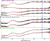 |
Fig. 1 Normalised-to-peak-flux spectra of our sample of millimetre-compact discs. The red line indicates the estimated continuum. The indicated types and their meaning are discussed in Section 5.1. In blue, we highlight the 23.72–24.03 µm wavelength region, where two transitions are located that are most important for obtaining information about the cold H2O reservoir. |
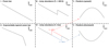 |
Fig. 2 Schematic highlighting the different parametric models used for the column density profiles. Both the horizontal (radius) and vertical (column density) axes are taken in log10-space. |
3.1 Rotational H2O spectrum: Parametric analysis
In an attempt to parametrically describe the observed H2O emission, we followed the approach from Romero-Mirza et al. (2024), whereby 50 slab models are used to sample profiles in both temperature and column density as a function of the emitting radius. As opposed to Romero-Mirza et al. (2024), we chose to first determine the radius as a function of temperature,
 (1)
(1)
This relation ensures that the inner radius (Rin (in au), as listed in Table 1) of our slab models is located at the estimated dust sublimation radius at 1500 K. Using this equation, we sampled the annular emitting regions of our 50 slab models for temperatures between 1500 K (the dust sublimation radius; Barvainis 1987) and 150 K (the condensation temperature of H2O; Collings et al. 2004) in log10-space. The dust sublimation radius was calculated following the approach of Dullemond et al. (2001),  . Both the calculated inner radii and adopted stellar luminosities can be found in Table 1. By simply rewriting Equation (1), we obtain a relation for the temperature as a function of the radius,
 (2)
(2)
For the column density, we used the same profiles as Romero-Mirza et al. (2024): a power law (profile I, Equation (3)) and an exponentially tapered power law (profile II, Equation (4)). In addition, we also tried different profiles. Figure 2 provides a schematic overview of the different profiles and their potential behaviours. In particular, we assumed a constant number of molecules (𝒩mol) with radius, whereby each annulus contains the same number of molecules, which automatically resembles a power law with a power of –2 (the emitting area, A, is proportional to the square of the radius). We then allowed this number of molecules to experience a jump; namely, the number of molecules would get enhanced (or depleted) by a factor, Fscale, at temperatures below a given jump temperature, Tjump (see Equation (5)). We tried profiles with a fixed jump temperature, at 400 K (profile III) and we kept Tjump as a free parameter (profile IV). The value of 400 K approximately resembles the boundary temperature between the sublimated (colder temperatures) and gas-phase-formed (hotter temperatures) H2O vapour reservoirs (see also Romero-Mirza et al. 2024). The jump temperature can move to higher temperatures, indicating a potential depletion of the hot H2O reservoir, or to colder temperatures, representing a potential enhancement of the cold H2O reservoirs. A parabola provides a smoother description of this behaviour: the jump moving to higher temperatures is captured by an upward parabola (the parabola has a maximum), while a downward parabola (the parabola has a minimum) captures the behaviour of the jump moving to lower temperatures (see also Figure 2). Therefore, we fitted a parabola in log space (profile V, Equation (6)). The equations describing the column density profiles of each of these cases are:
 (3)
(3)
 (4)
(4)
 (5)
(5)
 (6)
(6)
The emitting area of each slab model is accounted for in the exact same manner as reported in Romero-Mirza et al. (2024). The area is multiplied by the cosine of the disc’s inclination (i, reported in Table 1),  , where R1 and R2 are, respectively, the inner and outer radii of each annulus (see also Equation (1)).
We fit the profiles, sampled by the 50 slab models, using a Markov chain Monte Carlo (MCMC) approach, implemented through the EMCEE python-package (Foreman-Mackey et al. 2013). From the posterior distribution of the MCMC, we take the median values as the best-fit values for the fitted parameter. Additionally, the 18th and 84th percentiles are taken as the lower and upper 1σ uncertainties. We use a reduced-χ2 as the likelihood function of the MCMC, in order to compare the full model (the sum of the 50 slab models) with the observations. The likelihood has, therefore, takes the following form:
 (7)
(7)
where Fobs is the observed spectrum and Ndata is the number of data points within the used fit regions. Then, σ denotes the noise of the observations, determined in a similar manner as in Temmink et al. (2024b), where the James Webb Exposure Time Calculator1 has been used to obtain the continuum signal-to-noise (S/N) at the midpoint of each sub-band given the observational setup. The S/N values are given in Table B.1. As the noise is significantly higher in Channel 4 and many important H2O lines can be found at these wavelengths, we slightly offset the large noise by introducing weights in the χ2-formula, wi. All fit regions beyond 20 µm have been given a higher weight of 5, while select regions with important transitions probing the cold reservoir have been given a weight of 10 or 15 (for the strongest transitions). While the values are arbitrary, these weights ensure that we are able to properly fit the full rotational spectrum, without favouring the hot reservoir, as the transitions at smaller wavelengths have lower flux uncertainties. Fits without any weights favour the hot reservoir. Therefore, the chosen weights ensure that our models properly fit all reservoirs, including the cold one that is best probed by the longer wavelengths that are more noisy given the lower sensitivity of JWST/MIRI’s Channel 4. While the choice for the weights is arbitrary, using lower weights will still favour the hotter reservoirs and result in a worse fit for the colder reservoir, whereas higher weights may start overrepresenting the cold reservoir and result in worse fits for the hot one.
In the MCMC, we used 20 walkers per free parameter and allowed the MCMC to explore the prior space for 50 000 iterations. Table 2 lists the prior spaces for each profile. Common priors that are kept the same in each fit are only listed once, for example, the number of molecules, Nmol, in the jump abundances. For some sources, we ran a second fit with a more limited prior space. In these cases, a second, less favourable solution was often found and a number of walkers got stuck in this local minimum, not allowing the fit to converge. The updated prior space was subsequently chosen to exclude these local minima. All fits use selected isolated H2O lines and ortho-para line pairs, which all have been taken from Banzatti et al. (2025) (see their Figure 3 and Tables 5 and 6). The applied fit regions, which were also shifted by the heliocentric velocity, are listed in Table C.1. We used fewer regions for CX Tau and DN Tau, as the CO2 P- and R-branches strongly contribute to their observed emission.
Priors used for the profiles listed in Section 3.1.
3.2 Rotational H2O spectrum: Multiple components
As a comparison, we also followed Temmink et al. (2024a) to investigate the pure rotational H2O spectrum using two (in the case of CX Tau and DN Tau) or three slab model components. Through trial and error (i.e. by fitting three or two components), we found that only two components were needed to fully describe the rotational H2O spectra of CX Tau and DN Tau. This is very likely due to the H2O emission being much weaker compared to the other sources (see Figure 1). We did not use all three approaches presented in Temmink et al. (2024a), but only the simplest one, approach I, which assumes a simple radial gradient. The line optical depths are sufficiently high that the vertical gradient in approach III does not matter and the results resemble those of approach I.
To agree with the parametric analyses discussed in Section 3.1, we slightly adapted approach I: instead of having a circular area surrounded by two annuli, we use three annuli with the inner radius of the first set to the dust sublimation radius, Rin. The other two or three radii are kept free, together with their respective temperatures and column densities. Therefore, Equation (2) of Temmink et al. (2024a) becomes:
 (8)
(8)
For the sources for which we only fit two components, the third term in the above equation can be ignored.
The fits were done using the same MCMC setup, with the same reduced-χ2 formula taken as the likelihood (see Equation (7)), as in Section 3.1. The same fit regions are used for the most optimal comparison between the results.
3.3 Line flux ratios
Aside from analysing the spectrum through slab models, we followed Banzatti et al. (2025) and analysed their suggested line flux ratios: F1500 K/3600 K and F3600 K/6000 K (see also the rightmost panel in their Figure 10). In particular, these line ratios will provide information on, respectively, the cold and hot H2O vapour reservoirs. The temperatures indicate the approximate upper level energy. The 1500 K flux is comprised of two isolated H2O transitions, with upper level energies of, respectively, 1448 K (at λ=23.81676 µm) and 1615 K (at λ=23.89518 µm), while the 3600 K and 6000 K fluxes are taken to be the isolated lines at 17.50436 µm and 17.32395 µm. Given their upper level energies, these lines probe the strength of the different temperature reservoirs and the ratios provide insights into the potential enhancement of the cold reservoir. Following Banzatti et al. (2025), we take the sum from the line fluxes of the 1448 K and 1615 K transitions as the total value for F1500 K. To determine the line fluxes, we followed the approach of Banzatti et al. (2012) and Temmink et al. (2024b), based on the techniques provided by Pascucci et al. (2008), Najita et al. (2010), and Pontoppidan et al. (2010): we obtained a Gaussian distribution of measured line flux, using 1000 iterations of adding normally distributed noise (following the S /N values in Table B.1), by fitting Gaussians (using the python-package LMFIT, Newville et al. 2024) to the lines. From these distributions, we took the median value as the line flux and the full FWHM as the uncertainty.
4 Results
In the following section, we highlight the results from our different fitting methods. In Section 4.1, we present the parametric results for the different fit profiles, while the results of the multiple-component analysis are shown in Section 4.2. The calculated line fluxes for the different line tracers are displayed in Section 4.3.
4.1 Parametric analysis
Figure 3 displays all fitted profiles for our sample of compact discs with a line width of 4.71 km s−1. Those for the quadrature line widths are given in Figure D.1. Given the profiles, we find three groups of discs: BP Tau, CY Tau, DR Tau, and RNO 90 all behave very similarly, which is most notable in the exponentially tapered power laws (second column), the jump abundances with Tjump at higher temperatures (Tjump ≳ 650 K, fourth column), and the resulting upward parabolas (fifth column). The resulting profiles for FT Tau and XX Cha are also nearly identical, but differ from the other four sources. The jump abundance occurs at a low temperature of Tjump ≤ 250 K for these discs, while their power laws are very slowly declining and their downward parabolas are very shallow. Finally, aside from their very similar spectra (see Figure 1), the parametrisations of CX Tau and DN Tau also behave very similarly to each other, but are different from the other discs. Their jump abundance occurs at the intermediate temperatures Tjump ∼ 500–600 K, while their power laws are monotonically increasing with radius and their parabolas are turned downwards.
The  values are listed in Table D.1, where we have highlighted the parametrisations with the lowest
  -value in boldface. Figures D.2–D.9 compare these best-fitting models with the observations and the fitting parameters are also listed in Tables D.2 and D.3. These tables also include uncertainty values on the retrieved fitting parameters. Those uncertainties are taken as the 16th and 84th percentiles of the posterior distributions and, therefore, represent the 1σ upper and lower limits, respectively. From the
  values, it is clear that not one single parametrisation provides the best description of all observations. Instead, a combination of the different profiles is preferred. We also note that the
  values of the different parametrisations are overall very similar.
Finally, we briefly highlight the resulting temperature slopes (values for q, see Equations (1) and (2)) according to our retrieved profiles. From Tables D.2 and D.3 it is clear that our retrieved values of q are between 0.35 and 1.30. Overall, we find the lower values for BP Tau, DR Tau, FT Tau, RNO 90, and XX Cha, while the higher values are found for CX Tau, CY Tau, and DN Tau. The average of the best-fitting parametrisations for all discs suggests a power law slope of q ∼0.57 for the temperature, which is somewhat lower than the value found by Romero-Mirza et al. (2024) of q ∼ 0.69 and the value suggested by thermochemical modelling of q ∼ 0.7 in the surface layers of discs (Bosman et al. 2022, Vlasblom et al., in prep.). Our average value would be even lower if we had only accounted for the results from the quadrature line widths.
4.2 Multiple component analysis
Overall, we find rather good agreement between the best-fitting profiles and the multiple components (three or two), as can be seen in Figures 3 and D.1, where the discrete data points indicate the results of such fits. The resulting values are given in Table D.4, while the  values are also listed in Table D.1. We note that the radial locations shown in Figures 3 and D.1 are not the values for R1, R2, and R3, the outer edge of each emitting area, but these are the central values of each emitting area. The resulting spectra for the best-fitting models are also included in Figures D.2–D.9 (red profiles).
The results for the multiple-component analysis are rather similar between the different discs with either three or two components fitted: for the three-component fits, we find that the temperatures for the first component all fall in the 765–970 K range, while those for the second and third components fall in the respective ranges of 355–530 K and 200–300 K. We note that the temperatures of the second and third components for FT Tau and XX Cha (T2 ∼ 385 and T3 < 215) are lower than those for BP Tau, CY Tau, DR Tau, and RNO 90, further suggesting a difference in behaviour as seen for the parametric analysis in Section 4.1. The temperatures for CX Tau and DN Tau, where only two components were fitted, are also very similar. The first component has a temperature between ∼ 400–500 K for both sources, with slightly higher temperatures for DN Tau, while the second component has a temperature in the range of 190–240 K.
Similarly, the column densities follow the same structure, where generally the first component has the highest column density, followed by the second and the third (where applicable). We note, however, that the retrieved column densities cannot be assumed to lie on a simple power law: as can be seen in Figure 3 and D.1, the other parametrisations provide better agreement with the multiple-component fits. For example, the downward parabola structure of CX Tau and DN Tau cannot be captured by a power law through the individual components. Finally, the high values for the emitting areas of the third component very likely indicate optically thin emission (see also Temmink et al. 2024a).
4.3 Line flux ratios
The values for the derived line fluxes are given in Table F.1, while the ratios are displayed in Figure 4, which has been adapted from Banzatti et al. (2025) (see their Figure 10, right panel) to include our sample of compact discs (the coloured data points). The grey data points are those from Banzatti et al. (2025), using the values listed in their Table 3. We find that BP Tau, CY Tau, DR Tau, and RNO 90 show similar line flux ratios as the sample of Banzatti et al. (2025), while the line fluxes of the cold lines (F1500K) are much stronger in FT Tau and XX Cha. CX Tau and DN Tau also appear to have higher cold line fluxes, but we note that their hot H2O line fluxes (F6000K) are significantly lower. The implications of the locations of the different discs in Figure 4 are further discussed in Section 5.1.
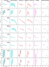 |
Fig. 3 Profiles and multiple components (right-most panel) fitted for our sample of compact discs using a line width of 4.71 km s−1. The shaded area is the 1σ-confidence interval, given the uncertainties listed in Table D.2. The red stars in the top-left corner indicate the best fitting profiles for each disc (see Table D.1). We note that the best-fitting profile for DN Tau is highlighted in Figure D.1. |
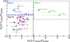 |
Fig. 4 Ratios of the 3600 K/6000 K and 1500 K/3600 K line fluxes, used to investigate the respective strength of each H2O reservoir. The grey data points are adapted from Banzatti et al. (2025) (see their Table 3), where we have highlighted those analysed by Romero-Mirza et al. (2024) and potential type P sources (i.e. MY Lup, RY Lup and IRAS-04385). The coloured data points indicate the line ratios of our sample of compact discs. See Section 5.1 for a discussion on the different types. |
5 Discussion
In the following sections, we discuss and interpret our results. From our analysis, it immediately becomes clear that these discs, even though they are all classified as compact, show different behaviours given their H2O spectra and inferred H2O distributions. Not all of these discs show a strong, enhanced cold H2O reservoir, suggesting that additional factors are at play within these systems. Within our sample of compact discs, many of them may behave just like large and structured discs, while only a limited number actually show cold H2O emission to be strongly enhanced, likely due to radial drift.
5.1 Profile types and H2O reservoirs
Given the different observed behaviours (see Section 4.1) and the observed line fluxes, we propose to categorise planet-forming discs in at least three different types, based on their H2O reservoirs: type N, type E, and type P (as already highlighted in Figures 1 and 4). Type N includes the ‘normal’ discs, which show all three H2O reservoirs (hot with T > 800 K, intermediate with 400 < T < 800 K, and cold with T < 400 K). The cold reservoir is present following the temperature gradient, expected to be present in all discs, but not strongly enhanced suggesting that radial drift is not efficiently replenishing the inner disc with icy pebbles. These discs can be found in the lower-left corner of Figure 4, where both ratios (F1500 K/F3600 K and F3600 K/F6000 K) have low values. We expect many of the large and structured discs to be part of this category.
The type E discs include those with very strong cold H2O gas reservoirs, which appear to be significantly enhanced, suggesting efficient radial drift. These discs can be found in the top left corner of Figure 4, indicating their large cold H2O reservoirs by large values for F1500K/F3600 K, while their values for F3600K/F6000K are similar to the type N discs. Finally, type P indicates the H2O-poor (or CO2-rich; Pontoppidan et al. 2010; Vlasblom et al. 2025) discs, whose spectra are generally devoid of H2O, but still show strong emission from the cold reservoir. Emission from the other two components is often found to be weak and the emission present can be fitted with either a hot or an intermediate temperature. The lack of H2O emission from both components (i.e. strong emission from both hot and intermediate) could potentially be due to a small inner cavity depleting the reservoirs in these components (Grant et al. 2023; Vlasblom et al. 2024). The cold component could still be prevalent due to radial drift, especially since snowlines are pushed further out in discs with cavities, holding for both the inner and outer regions (Temmink et al. 2023; Vlasblom et al. 2024). These H2O-poor discs can be found in the top right corner of Figure 4, with high values for both F1500K/F3600K and F3600K/F6000K. We note that the boundaries for the different types in Figure 4 are arbitrary. To empirically determine the boundaries between the different types, a larger number of discs needs to be consistently analysed. We leave this for future work (Temmink et al., in prep.).
Based on our analysis of the 8 compact discs in the MINDS sample, we suggest that BP Tau, CY Tau, DR Tau, and RNO 90 can all be considered as type N discs, while FT Tau and XX Cha are the only two compact discs with very strong cold H2O reservoirs: we consider them to be type E discs. CX Tau and DN Tau are considered to be type P discs. Using this categorisation we suggest that the type N discs can best be described (that is, lowest  -values) by profiles with jump abundances at higher temperatures or upward parabola, which also resembles the power law profile with a strong exponential taper. The type E discs are the ones with a jump abundance occurring at low temperatures (T < 250 K), have slow monotonically decreasing power laws, and may be described by a shallow downward parabola. On the other hand, the type P discs likely have rising power law profiles or jump abundances occurring at intermediate temperatures. Furthermore, their parabolas have a strong minimum.
The distinction between the different groups also becomes visible when investigating the contribution (with respect to the maximum flux in the observed spectrum) of the 50 individual slab models within the different profiles. As we are fitting 50 different slab models, if they all contributed equally, they would each reach a maximum contribution of 2% at every wavelength. Figure 5 displays the flux contribution of the slab models for DR Tau (top panel: type N), FT Tau (middle panel: type E), and CX Tau (bottom panel: type P). The contributions for DR Tau show that the hot component is the weakest (≤ 1.5%), as expected from the upward parabola, while the intermediate and cold reservoirs are of similar strength (∼ 3–4%) given the increasing emitting areas with decreasing temperature. For FT Tau, the hot and intermediate reservoirs are of similar strength (∼ 2%), while the cold reservoir has the strongest contribution (≤ 6%). The contributions for CX Tau show similar strengths in the hot and cold H2O reservoirs (≤ 8%), but a negligible intermediate component, as expected from the downward parabola. While slab models probing the hot and cold reservoirs may have similar maximum contributions, fewer hot H2O slabs contribute this much to the spectrum and the spectrum is dominated by the cold reservoir overall. Additionally, we want to emphasise that the best-fitting profile dictates the outcome of Figure 5: while the contributions for CX Tau, because of the parabola, have a strong contribution of the hot component, those of DN Tau (both type P discs) will lack the hot component and have significant contributions from the intermediate component as the spectrum is best-fitted by a jump abundance at a temperature of Tjump ∼ 600 K. Finally, we note that the line-to-continuum ratio of CX Tau is much lower (factor of ≥5) than for the other two sources, highlighting that even the higher percental contributions may not be as noticeable as for the other sources.
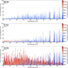 |
Fig. 5 Contributions of each individual slab model with the colour representing the excitation temperature of the respective slab. The contributions are shown for the best fitting parametric models of DR Tau (type N), FT Tau (type E), and CX Tau (type P). The contributions are taken as the percentage with respect to the maximum line flux in the full model. We note that the maximum line flux of CX Tau is at least a factor of 5 lower than that of the other two types. |
5.2 Role of sub-structures
With our sample of compact discs now categorised, we highlight that the analysis of the ALMA visibilities of some of our sources has suggested that these rather compact discs may harbour sub-structures. In particular, gaps and rings have been proposed for the outer regions (>15 au) of BP Tau (Jennings et al. 2022; Zhang et al. 2023; Gasman et al. 2025), DN Tau (Long et al. 2018; Zhang et al. 2023), DR Tau (Jennings et al. 2022; Zhang et al. 2023; Gasman et al. 2025), and FT Tau (Long et al. 2018; Jennings et al. 2022; Zhang et al. 2023). With sub-structures hypothesised in discs across all three types, it is clear that the role of sub-structures in setting the inner disc H2O reservoirs is not yet well understood (see also Gasman et al. 2025). Furthermore, as modelling works have shown that the influence depends on the gap location, the time at which the structure formed, and how leaky the traps are, this implies that sub-structures may play a very diverse role in setting the inner disc reservoirs (Kalyaan et al. 2023; Sellek et al. 2025; Easterwood et al. 2024). Age may also play a role (Mah et al. 2023), but we note that the majority of our sample consists of sources from the Taurus star-forming region and it can, therefore, be assumed that these discs all have a similar age. Therefore, our sample may be rather homogeneous and a larger sample, consisting of sources from a variety of different star-forming regions and with different ages, is needed to not only investigate the role of the structure formation time, but also the drift timescale (Mah et al. 2023, 2024).
Our introduced types may, therefore, be comprised of a wide variety of discs. Higher-resolution ALMA observations (spatial resolution of <0.1′′, but preferably as high as possible) and observations with infrared observatories are needed to confirm and further study these sub-structures and their potential roles in setting the inner disc abundances, as well as hunt for sub-structures at smaller scales.
5.3 Profile implications
The following section discusses the differences in more detail. In particular, we further highlight the behaviours of the profiles and what this implies. In Appendix G, we also discuss how well the different profiles fit each type.
For the type N discs, we find that all discs prefer a jump abundance at higher temperatures of generally Tjump ≳ 700 K or a downward parabola (maxima generally at temperatures above 600 K). This behaviour suggests a potential depletion of the hotter component with respect to the stronger intermediate and cold components. This ‘depletion’ could simply mean that the hot H2O reservoir is not as abundant as the intermediate and cold ones and, therefore, does not follow a simple power law profile, but it may also have a more physical explanation. As suggested by theoretical models (Sellek et al. 2025; Houge et al. 2025), the inward drift of icy pebbles not only increases the molecular reservoirs when crossing the snowlines, but also increases the continuum optical depth (τ) and, therefore, the continuum τ=1 layer may be moved to higher layers and obscure the underlying H2O reservoirs.
On the other hand, the optical depth of the H2O lines themselves may play an important role, which could reach values of τ ∼ 3000 (Temmink et al. 2024a). Therefore, it is possible that only the very top region of the emitting layer can be probed, well above the dust continuum τ=1 layer, while the remainder of the reservoir remains invisible given the high optical depths. As the line optical depth is found to be higher for the hottest component compared to the cooler components (Temmink et al. 2024a), this may play an important role in setting the observable column density for H2O in the innermost region.
Finally, the destruction of H2O could also play a role in depleting the inner regions. One of the main destruction routes in these high atmospheric layers of discs is photodissociation. The photodissociation must, however, occur on timescales faster than the gas-phase formation, which is efficient at >300 K (Bosman & Bergin 2021), to effectively destroy H2O. Additionally, H2O can be destroyed in these layers through collisions with C+, Si+, and H+ (Kamp et al. 2013). There is no consensus on which explanation for the flattening of the profiles in the inner regions is correct, as it may be a combination of all three: dust obscuration, optical depth, and destruction. We expect that it is more than likely that different combinations are preferred by different discs and the importance of each explanation will also differ.
The type E discs, FT Tau and XX Cha, have most notably the jump abundance at low temperature (Tjump < 250 K) or a shallow downward parabola. As drift can be expected to play to a certain extent a role in all discs, both smooth and structured, where the leakiness of the sub-structures determines the inward flow of material (Mah et al. 2023, 2024; Gasman et al. 2025), the cold component should be present in most if not all discs. The strength of the cold component in FT Tau and XX Cha, and therefore the jump in abundance at Tjump ∼ 250 K and the slowly decreasing power law, can be explained by an extreme or very efficient inward flux of the icy pebbles, enhancing the abundance of this cold component near the H2O snowline with respect to the other discs.
We note that not all discs in the type E category may undergo efficient radial drift. Instead, an accretion outburst that significantly heats up the disc and, therefore, enlarges the emitting area of the cold component may also result in discs falling into this category. In particular, it has been found that XX Cha is highly variable in its accretion (Claes et al. 2022). Even though its variability timescales have not yet been constrained, the observed variation with the X-shooter instrument is on a scale of almost 2 dex (i.e. a factor of 100). Therefore, the strong cold component of XX Cha may be due to its strong variable accretion instead of efficient drift. Furthermore, recent work attributed the strong cold H2O reservoir observed in the disc of EX Lup to an accretion outburst and the subsequent sublimation of H2O ice, given the snowline being pushed outwards (Smith et al. 2025). For FT Tau, the other disc identified as a type E disc in our sample, there are currently no claims of accretion outburst or a strongly variable accretion rate. The reported accretion rate for FT Tau gives values between log10  (Garufi et al. 2014; Gangi et al. 2022) (with
  given in M⊙ year−1), but have not been monitored closely over time. To confirm the role of accretion outbursts and variability in setting the inner disc chemical reservoirs, the accretion rates need to be monitored over an extended period of time to also infer the variability timescales. Also, if present, a larger sample of these sources needs to be observed with JWST-MIRI/MRS and analysed in a consistent manner.
The preferred parametrisations of CX Tau and DN Tau, the type P discs, include a monotonically increasing power law, a jump abundance at the intermediate temperatures, and a downward parabola. These profiles all imply a depletion of the hot or intermediate H2O component with respect to the colder reservoir, which is clearly the strongest. This may suggest a potential dust and gas cavity (see, for example, Salyk et al. 2025), where the cold H2O is most prominent due to sublimation of H2O ice near the cavity edge (see also Vlasblom et al. 2024).
Finally, we note that Banzatti et al. (2023a) described two compact discs (GK Tau and HP Tau) having an ‘excess’ in their cold H2O reservoir with respect to a large and structured disc (CI Tau). Here, we find that similar line flux ratios, as for their two compact discs and for our type N discs, do not necessarily imply an enhancement of the cold H2O reservoir, but rather a smooth distribution from hot and/or warm to cold. A true enhancement, as found for our type E discs, produces an even stronger excess in the cold H2O lines with respect to their warmer or hotter counterparts. This may also imply that CI Tau is actually depleted in the cold H2O and, therefore, falls to the lower left corner of Figure 4. Therefore, the type E compact discs of FT Tau and XX Cha most closely conform with the hypothesis posed by Banzatti et al. (2020) and the overall situation appears to be more complex.
Overall, we find that the jump abundance with the jump temperature (Tjump) kept free is amongst the favoured fit for all three types. Therefore, we suggest that this profile can be fitted to investigate the H2O reservoirs in all discs. Furthermore, the location of the jump, as discussed for each type above, may suggest which type the disc belongs to.
5.4 Line width comparison
One aspect that has not yet been addressed relates to the choices made for the different line widths, namely, between a fixed value of 4.71 km s−1 or the sum in quadrature of a fixed turbulent line width and the thermal line width, given the temperature of the slab model. Intuitively, the quadrature line profiles may be preferred, as the line width changes accordingly with the temperature. One downside is that the strength of turbulence is not known in the inner regions of these discs, therefore, the turbulent component of the line width (fixed to 1 km s−1) may be stronger or weaker. Thus far, a few studies have measured the turbulence in the outer regions of large discs using ALMA, resulting in values of <0.2 km s−1 (Paneque-Carreño et al. 2024) or up to ∼ 35% of the sound speed (<0.35cs; Flaherty et al. 2015, 2017, 2020). We find that seven out of eight of our discs prefer the fixed value of 4.71 km s−1. This may suggest that the inner regions of these discs are more turbulent and higher values need to be assumed for the turbulent component (ΔVturb > 1.0 km s−1).
The preferred larger line width may be related to the change in the optical depth of the lines, which decreases with larger line widths (τ ∼ N/ΔV, with ΔV the line width). As the quadrature line widths are generally smaller (see also Romero-Mirza et al. 2024), these models will have larger optical depths. Furthermore, it becomes apparent from the contribution plots (Figures G.1–G.2) that the quadrature line profiles have stronger fluxes in certain lines of the cold component (see, for example, transitions around 25.05 or 26.70 µm). Given the added weights to the lines fitted at the longest wavelengths (>20 µm), we expect the fitting method to find the best profile describing the observed spectrum, regardless of the lower sensitivity of the larger wavelengths observed with JWST-MIRI. Therefore, it is possible that the cold component of the majority of our sample is less optically thick compared to the other discs.
Finally, we notice that our profiles show no qualitative differences between the different line widths (see Figures 3 and D.1), except for the parabola of DN Tau, which changes between upward and downward. Therefore, we conclude that the choice of line width does not really matter for the profiles, but note that the optical depth of the reservoirs, as discussed above, does depend on the chosen line width.
5.5 Comparisons with previous analyses
In this section, we compare our analysis with the works of Romero-Mirza et al. (2024) and Gasman et al. (2025), who, respectively, fitted (tapered) power-laws to seven other discs and analysed the H2O emission in ten structured discs. Additionally, we compare our results with the interpretation of the models by Houge et al. (2025).
Romero-Mirza et al. (2024) only used power law and tapered power law profiles (our profiles I and II) to fit the column density distributions of four compact discs (FZ Tau, GK Tau, GQ Tau, and HP Tau) and three larger discs (AS 209, CI Tau, and IQ Tau). They find that all these discs can be well described by a simple power law, while both CI Tau and FZ Tau prefer the exponentially tapered power law, potentially suggesting a ring-like distribution of the H2O reservoir. All discs are also captured in the analysis of Banzatti et al. (2025) and are, therefore, displayed in Figure 4, in which we have highlighted their respective positions. All of them, except for maybe GQ Lup, fall within our selection of type N discs. GQ Lup may also be a type N disc, given that it is located towards the lower right of Figure 4 with respect to FT Tau and XX Cha and has, therefore, a stronger intermediate component. As stated before, the current definition of the types on Figure 4 is somewhat arbitrary and refining the boundaries for each disc type requires a larger sample of sources, which will be addressed in future work (Temmink et al. in prep.). We also cannot exclude the possibility that other behaviours and types may exist outside the parameter space covered by the eight discs in our sample. As all discs analysed by Romero-Mirza et al. (2024) may be type N discs, their profiles can indeed be described by power laws (similar to CY Tau), but may also be represented by jump abundances at higher temperatures or upward parabolas.
Gasman et al. (2025) compared a sample of 10 structured discs and put their H2O emission in context with respect to DR Tau. They note that the H2O reservoirs are complicated for these structured discs and that the H2O reservoirs strongly depend on the age of the system, the mechanisms that open a gap in the outer disc, and the leakiness of such sub-structures (see also Mah et al. 2024). We note that BP Tau and DR Tau are the two discs overlapping between their sample and ours, highlighting that compact discs may be structured as well. Relative to DR Tau, there is a distinct group of large, structured discs (CI Tau, DL Tau, GW Lup, and V1094 Sco) that have a weaker cold H2O reservoir, which may end up in the lower left corner of Figure 4, where the position of CI Tau is already high-lighted. Another group of structured discs (SY Cha and Sz 98) shows, on the other hand, a very strong cold component (stronger than DR Tau) and may, therefore, end up in the upper left corner of Figure 4 near FT Tau and XX Cha. This suggests that the H2O reservoirs of planet-forming discs are much more complicated and one cannot simply separate them into different types based on their size and/or dust structures, as already discussed in Section 5.3.
Finally, we compare our best-fitting profiles to the predicted model column density profiles by Houge et al. (2025) (for a star with L∗=4 L⊙, see Figure 6). Their column density profiles are given for the observable H2O reservoir above the τ=1 layer at 20 µm. Their predictions are given for a fixed ratio between the chemical and mixing timescales (tchem/tmix=0.01) or for a fixed chemical timescale (tchem=10 years) with a radially varying mixing timescale. Furthermore, their models include three types of dust models: fragile (vfrag=1 m s−1), composition-dependent (vfrag=1–10 m s−1), and resistant (vfrag=10 m s−1). They find that for sufficient fragile dust (i.e. in the fragile or composition-dependent cases) the column density is set by the vapour-to-dust mass ratio and the dust opacity, as the profiles for those models do not strongly depend on any disc properties and, therefore, do not evolve over time (see also Sellek et al. 2025). While a direct comparison with the models of Houge et al. (2025) cannot be made given the stellar parameters used in their models, we compare the overall shape of the models with our best-fitting column density profiles in Figure 6. In particular, we make the comparisons with the models with a fixed chemical timescale and radially varying vertical mixing for the different dust types at a time of 1 Myr, an appropriate assumed age for the majority of our sources (see, for example, Krolikowski et al. 2021; Luhman 2023).
Qualitatively, the models and observations agree in the sense that the column density profiles decrease towards larger radii. However, our profiles decrease or flatten off towards the inner regions (see, for example, DR Tau and RNO 90). This could be due to the fact that the expression used by Houge et al. (2025) to derive the abundance of water in the surface layers assumes that the chemical timescale (i.e. the destruction timescale) is always much shorter than the mixing timescale. Under their assumptions, the abundance should saturate inside 0.16 au at a level equal to that of the midplane, resulting in the profile flattening off. This level, namely the limit of N ∼ 1020 cm−2 explored by Sellek et al. (2025), would be equivalent to negligible destruction under the assumption that the H2O and dust particles behave the same and on similar timescales (that is, as long as the dust is not depleted on faster timescales than the H2O). Our best-fitting profiles, except for the outer regions of CX Tau, do not exceed a column density of N ∼ 1020 cm−2, which is in agreement with the limit proposed by Sellek et al. (2025).
Quantitatively, the retrieved column densities fall below all the model profiles for many of our sources, even for the most conservative model predictions with the fragile dust. On the one hand, while their expected column density profiles are based on the increased dust obscuration following radial drift, the importance of the optical depth of the H2O lines themselves is not explored, which may be important (as discussed in Section 5.3). Alternatively, this may suggest that for our sample of discs, the ratio of the chemical and mixing timescales is smaller than their assumptions. This may result from shorter photodissociation timescales, which are typically expected to be <1 year in the upper most layers of the disc (Bosman & Bergin 2021, Vlasblom et al. in prep.) and depend source-by-source on the stellar properties (i.e. the UV irradiation field). This may suggest that a chemical timescale of tchem=10 yr may be too long. Future 2D models should further investigate the physical and chemical processing of H2O in the inner regions and explore how effective the combination of increased dust obscuration following radial drift and line optical depth is.
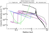 |
Fig. 6 Comparisons between our parametric models with the lowest |

Summary of the other molecules detected in our sample of discs.
5.6 Other molecular species
While our analysis focuses solely on the H2O emission, the spectra of these compact discs contain more molecular species. In this section, we only highlight the other molecular species detected and leave the analysis of this emission for future work. We start by noting that CX Tau (Vlasblom et al. 2025) and DR Tau (Temmink et al. 2024b,a) have dedicated papers analysing their molecular emission and we, therefore, refer the reader to these papers. For the other discs in our sample, the commonly observed species (OH, CO2, HCN, and C2H2) are detected in nearly all discs. For some discs, we also report the (potential) detection of CH4 in CY Tau and that of some of the isotopologues, such as 13CCH2 in CY Tau and both 13CO2 and CO18O in DN Tau, which is very similar to CX Tau (Vlasblom et al. 2025). The different species detected in each disc are summarised in Table 3, while Appendix E contains a more elaborate discussion of the detected species.
6 Conclusions and summary
In this work, we analyse the pure rotational H2O JWST-MIRI/MRS spectra of 8 millimetre-compact dust discs. We expand upon existing techniques to provide detailed parametric profiles of the column densities beyond (exponentially tapered) power laws. This leads us to infer the best-fitting radial profiles and investigate whether these compact discs show signatures of enhanced reservoirs due to radial drift or whether the overall situation is more complex. Our main conclusions are summarised as follows:
The pure rotational H2O spectra of compact dust discs are very different from each other. Half of the discs show similar strengths for the different H2O reservoirs, conforming with what is seen among large and structured discs, while others show clear signs of an enhanced cold reservoir, even beyond that found in previous comparisons of compact and large discs;
Different combinations of parametrisations can be used to describe the observed reservoirs in different discs, leading to the conclusion that planet-forming discs can be grouped into at least three different types (N, E, and P), based on their mid-infrared H2O spectra;
The parametrisation that assumes a constant of number of molecules with radius (i.e. the column density is proportional to negative the square of the radius) and has a jump (either an enhancement or depletion) in the abundance at a free temperature is able to provide a good fit for the column density profiles for all discs. The temperature of the jump varies per disc but is found to be similar within each of the different types (N, E, or P);
We find that the column density profiles and, therefore, the distribution of the H2O reservoirs are generally best fitted with a fixed line width of ΔV=4.71 km s−1. As the quadrature sum is intuitively and physically more correct, this may suggest that the turbulence is stronger in the inner disc and, therefore, a larger value for the turbulent component needs to be assumed (ΔVturb >1 km s−1);
Overall, a good agreement is found between the column densities retrieved through a multiple-component analysis and the profiles obtained through the parametric models. The parametric models show that one cannot assume a simple power law through the column densities derived from a multiple-component fit, but it is recommended to fit one of the other parametric models used throughout this work.
This work has shown that not all millimetre-compact discs have signatures of strongly enhanced cold H2O reservoirs following radial drift. Instead, half of our sample behaves similarly to larger, more structured discs. Therefore, we have introduced a new categorisation, given the behaviour of the H2O reservoirs seen for our discs: type N, type E, and type P discs. Here, N stands for ‘normal’ discs, whose spectra have contributions from all the components (hot, intermediate, and cold). Type P discs are the H2O-poor discs, whose spectra are dominated by other molecular species, yet have a strong contribution from the cold reservoir. Finally, the type E discs are the ones that show enhanced cold H2O, which may be the result of the strong inward drift of icy pebbles or, perhaps, the product of an accretion out-burst that pushes out the H2O and increases the emitting area of the cold H2O reservoir. Only two of our eight compact discs fit into this final category, further highlighting that not all compact discs have enhanced cold H2O reservoirs. These three types provide a new classification of discs, purely based on their rotational H2O emission and may be used to further explore trends involving system properties. Higher resolution ALMA observations and/or observations with infrared interferometers are required to further study the occurrence of sub-structures in these discs, on small and large scales, and how they may affect the observable reservoirs.
Data availability
Figures D.2–D.9 can be found on Zenodo: https://zenodo.org/records/15479557.
Acknowledgements
The authors would like to thank the referee for many thoughtful, constructive comments that helped improve the manuscript. This work is based on observations made with the NASA/ESA/CSA James Webb Space Tele-scope. The data were obtained from the Mikulski Archive for Space Telescopes at the Space Telescope Science Institute, which is operated by the Association of Universities for Research in Astronomy, Inc., under NASA contract NAS 5-03127 for JWST. These observations are associated with program #1282. The following National and International Funding Agencies funded and supported the MIRI development: NASA; ESA; Belgian Science Policy Office (BEL-SPO); Centre Nationale d’Etudes Spatiales (CNES); Danish National Space Centre; Deutsches Zentrum fur Luft- und Raumfahrt (DLR); Enterprise Ireland; Ministerio De Economía y Competividad; Netherlands Research School for Astronomy (NOVA); Netherlands Organisation for Scientific Research (NWO); Science and Technology Facilities Council; Swiss Space Office; Swedish National Space Agency; and UK Space Agency. The data described here may be obtained from 10.17909/t6gq-q023. M.T., A.D.S., E.F.v.D., and M.V. all acknowledge support from the ERC grant 101019751 MOLDISK. D.G. thanks the Belgian Federal Science Policy Office (BELSPO) for the provision of financial support in the framework of the PRODEX Programme of the European Space Agency (ESA). E.F.v.D. also acknowledges support the Danish National Research Foundation through the Center of Excellence “InterCat” (DNRF150). E.F.v.D., I.K., and A.M.A. acknowledge support from grant TOP-1 614.001.751 from the Dutch Research Council (NWO). T.H., K.S. and M.S. acknowledge support from the European Research Council under the Horizon 2020 Framework Program via the ERC Advanced Grant Origins 83 24 28. A.C.G. acknowledges support from PRIN-MUR 2022 20228JPA3A “The path to star and planet formation in the JWST era (PATH)” funded by NextGeneration EU and by INAF-GoG 2022 “NIR-dark Accretion Outbursts in Massive Young stellar objects (NAOMY)” and Large Grant INAF 2022 “YSOs Outflows, Disks and Accretion: towards a global framework for the evolution of planet forming systems (YODA)”. G.P. gratefully acknowledges support from the Carlsberg Foundation, grant CF23-0481 and from the Max Planck Society. B.T. is a Laureate of the Paris Region fellowship program, which is supported by the Ile-de-France Region and has received funding under the Horizon 2020 innovation framework program and Marie Sklodowska-Curie grant agreement No. 945298. This work also has made use of the following software packags that have not been mentioned in the main text: NumPy, SciPy, Astropy, Matplotlib, pandas, IPython, Jupyter (Harris et al. 2020; Virtanen et al. 2020; Astropy Collaboration 2013, 2018, 2022; Hunter 2007; pandas development team 2020; Pérez & Granger 2007; Kluyver et al. 2016).
Appendix A Velocity shifted slab models
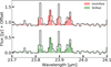 |
Fig. A.1 Comparison, using DR Tau as a test case, between an unshifted slab model (red) and one shifted by the heliocentric velocity. |
Appendix B S/N on the continuum and uncertainties for the observations
S/N values for each sub-band obtained from the Exposure Time Calculator.
Appendix C Slab model fit regions
Fit regions used for the fitting of H2O transitions.
Appendix D Fit results
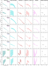 |
Fig. D.1 Similar to Figure 3, but for the quadrature line widths. The shaded area is the 1σ-confidence interval, given the uncertainties listed in Tables D.3. |
Summary of the results: 
Fit values for the profiles with a line width of 4.71 km s−1.
Fit values for the profiles with the quadrature line widths.
Fit values for the multiple-component fits.
Appendix E Other molecular species
In this following section, we discuss the observed molecular species, aside from H2O, in each disc (Section E.1) and we discuss the tentative detection of CH4 in CY Tau (Section E.2). These features are also highlighted in Figures D.2-D.9.
E.1 Molecules per source
BP Tau Aside from the pure rotational H2O lines, the spectrum of BP Tau also contains strong emission of the ro-vibrational transitions and CO emission at the shortest wavelengths (4.9-5.3 µm). Other molecular species, such as CO2 and HCN, are only weakly detected, while OH transitions are strongly detected above >15 µm. Both the H2 0-0 S(1) (at 17.30484 µm) and S(2) (at 12.27861 µm) are detected. The detected molecular species at >10 µm are also highlighted in Figure D.2.
CY Tau The strongest molecular feature in the spectrum of CY Tau belongs to C2H2, also visible in Figure 1. Its isotopologue, 13CCH2 is also well detected. Other molecular species include CO, the ro-vibrational lines of H2O, OH, HCN, and CO2. Both the H2 S(1) and S(2) transitions are also detected. Additionally, we present a potential detection of CH4 in this disc. The tentative detection is further highlighted in Section E.2. The molecular species are highlighted in Figure D.4.
DN Tau DN Tau has previously been classified, just as CX Tau, as a CO2-rich source (Pontoppidan et al. 2010). Aside from the strong emission of CO2, we report the detection of its isotopologue 13CO2 and the potential detection of CO18O. Other molecular species, such as HCN and C2H2 are not confidently detected, while OH is. At the shortest wavelengths, CO is only tentatively detected, while emission from the ro-vibrational H2O transitions is clearly detected. As for the other sources, both the H2 S(1) and S(2) transitions are also detected. Figure D.5 high-lights the detected molecular species.
FT Tau Aside from the strong pure rotational H2O emission, the spectrum of FT Tau also contains emission from the ro-vibrational lines and from CO. At the longer wavelengths, we clearly detect OH, CO2, HCN, and C2H2. The H2 S(1) and S(2) transitions are also detected. The emission of these species is also highlighted in Figure D.7.
RNO 90 Besides the rotational H2O transitions, the spectrum of RNO 90 also contains emission from CO, the rovibrational H2O transitions, OH, CO2, HCN, and C2H2. Both the S(1) and S(2) transitions of H2 are also detected. The molecular emission is highlighted in Figure D.8.
XX Cha Although the spectrum of XX Cha is very similar to that of FT Tau, the emission from both CO2 and C2H2 is stronger. Emission from CO, the ro-vibrational H2O lines, OH, and HCN are also clearly detected. As for all the other sources, both the H2 S(1) and S(2) transitions are also detected. Figure D.9 highlights the molecular emission of the other species in the spectrum of XX Cha.
E.2 Tentative detection of CH4 in CY Tau
We report a tentative detection of CH4 in the spectrum of CY Tau, whose Q-branch is located at ∼ 7.66 µm. In Figure E.1, we display the 7.60-8.00 µm wavelength region, containing molecular emission from ro-vibrational H2O transitions and potential weak features from C2H2 and the potential detection of CH4. For the slab models (H2O, C2H2, and CH4) we have used excitation temperatures of 975 K, 500 K, and 500 K, column densities (log10(N) with N in cm−2) of 18.4, 17.0, and 16.8, and emitting radii of 0.03 au, 0.10 au, and 0.10 au, respectively. The parameters for H2O and C2H2 were obtained using a  approach similar to that described in Section 3.1 but using grids instead of an MCMC exploration (see also, for example, Grant et al. 2023). The model for CH4 has been obtained by visually fitting the residuals. These slab models thus suggest a column density ratio of
  , under the assumption that the species are co-existing. The potential presence of CH4, in addition to the detection of 13CCH2, suggests that CY Tau may be the most carbon-rich disc in our sample. This disc may be similar to the much larger disc of DoAr 33, where Colmenares et al. (2024) reported, alongside other hydrocarbons, a tentative detection of CH4. They compared their spectra to thermochemical models and argued for an overall carbon-to-oxygen ratio (C/O) larger than unity.
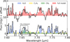 |
Fig. E.1 Zoom-in on the 7.60-8.00 µm region of CY Tau, showing the potential detection of CH4 (green). Also shown are approximate contributions from H2O (blue) and C2H2 (yellow) slab models. The full model is shown in red with a small offset applied to the flux. |
Integrated fluxes for the lines tracing the cold, intermediate, and hot H2O reservoirs.
Appendix F Integrated line fluxes
Appendix G Profile comparison
In Figures G.1, G.2, and G.3, we show the flux contributions of the 50 slab models for the profiles fitted for DR Tau, CX Tau, and FT Tau, respectively. These discs are each part of one of the different types and comparing their contribution plots provides information on how well the different profiles fit for their types.
DR Tau (type N) The type N discs (BP Tau, CY Tau, DR Tau, and RNO 90) are overall best described by the exponentially tapered power laws, the jump abundances with the jump occurring at high temperatures, and upward parabola (see also Table D.1). As can be seen in Figure G.1, those profiles all yield very similar contributions. The main differences between those profiles and the ones with the simple power law or the jump abundance with the jump fixed at Tjump=400 K is the flux at the shortest wavelengths (<15.0 µm), best probed by the hottest component, where the power law and the fixed temperature jump abundance have stronger contributions of the hotter components (most notable in the left panels of Figure G.1. These stronger contributions results in overfitting the observed flux in those inner regions, whereas the preferred profiles have a decrease in column density in the innermost and, therefore, do not overfit these inner regions.
FT Tau (Type E) FT Tau and XX Cha, the Type E discs, are best described by a jump abundance at low temperatures or parabola with a small upturn (see also Table D.1). As can be seen in Figure G.2 for FT Tau, the jump abundance with a jump at Tjump ≲250 K is really able to capture the strength of the cold component. The power law is not able to capture this cold component as strongly, but the contributions are clearly still there. The parabola, while being able to yield a similar contribution to the cold component as the power law, has a much stronger contribution at the shortest wavelengths (<15.0 µm) following its upward turn. This stronger contribution actually overfits the observed flux at these wavelengths, disfavouring the parabola as the best fit.
CX Tau (type P) The type P discs (CX Tau and DN Tau) mainly prefer the downward parabola and jump abundance profiles (see also Table D.1). As can be seen in Figure G.3, those profiles have the strongest contributions from either the hot or intermediate and cold components, while the (tapered) power law profiles are not able to capture the strength of all three components (hot, intermediate, and cold). The preference for these profiles shows that the P type discs do have contributions from at least two of the components.
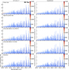 |
Fig. G.1 Contributions from all parametric fits for DR Tau, representing the type N discs. |
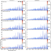 |
Fig. G.2 Similar as Figure G.1, but for FT Tau, representing the type E discs. |
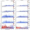 |
Fig. G.3 Similar as Figure G.1, but for CX Tau, representing the type P discs. |
References
- Ardila, D. R., Basri, G., Walter, F. M., Valenti, J. A., & Johns-Krull, C. M. 2002, ApJ, 567, 1013 [NASA ADS] [CrossRef] [Google Scholar]
- Argyriou, I., Glasse, A., Law, D. R., et al. 2023, A&A, 675, A111 [NASA ADS] [CrossRef] [EDP Sciences] [Google Scholar]
- Astropy Collaboration (Robitaille, T. P., et al.) 2013, A&A, 558, A33 [NASA ADS] [CrossRef] [EDP Sciences] [Google Scholar]
- Astropy Collaboration (Price-Whelan, A. M., et al.) 2018, AJ, 156, 123 [Google Scholar]
- Astropy Collaboration (Price-Whelan, A. M., et al.) 2022, ApJ, 935, 167 [NASA ADS] [CrossRef] [Google Scholar]
- Banzatti, A., Meyer, M. R., Bruderer, S., et al. 2012, ApJ, 745, 90 [NASA ADS] [CrossRef] [Google Scholar]
- Banzatti, A., Pontoppidan, K. M., Salyk, C., et al. 2017, ApJ, 834, 152 [NASA ADS] [CrossRef] [Google Scholar]
- Banzatti, A., Pascucci, I., Edwards, S., et al. 2019, ApJ, 870, 76 [Google Scholar]
- Banzatti, A., Pascucci, I., Bosman, A. D., et al. 2020, ApJ, 903, 124 [NASA ADS] [CrossRef] [Google Scholar]
- Banzatti, A., Abernathy, K. M., Brittain, S., et al. 2022, AJ, 163, 174 [NASA ADS] [CrossRef] [Google Scholar]
- Banzatti, A., Pontoppidan, K. M., Carr, J. S., et al. 2023a, ApJ, 957, L22 [Google Scholar]
- Banzatti, A., Pontoppidan, K. M., Pére Chávez, J., et al. 2023b, AJ, 165, 72 [Google Scholar]
- Banzatti, A., Salyk, C., Pontoppidan, K. M., et al. 2025, AJ, 169, 165 [Google Scholar]
- Barvainis, R. 1987, ApJ, 320, 537 [Google Scholar]
- Blevins, S. M., Pontoppidan, K. M., Banzatti, A., et al. 2016, ApJ, 818, 22 [NASA ADS] [CrossRef] [Google Scholar]
- Bosman, A. D., & Bergin, E. A. 2021, ApJ, 918, L10 [NASA ADS] [CrossRef] [Google Scholar]
- Bosman, A. D., Bergin, E. A., Calahan, J., & Duval, S. E. 2022, ApJ, 930, L26 [NASA ADS] [CrossRef] [Google Scholar]
- Bushouse, H., Eisenhamer, J., Dencheva, N., et al. 2024, https://doi.org/10.5281/zenodo.6984365 [Google Scholar]
- Carnall, A. C. 2017, arXiv e-prints [arXiv:1705.05165] [Google Scholar]
- Claes, R. A. B., Manara, C. F., Garcia-Lopez, R., et al. 2022, A&A, 664, L7 [NASA ADS] [CrossRef] [EDP Sciences] [Google Scholar]
- Collings, M. P., Anderson, M. A., Chen, R., et al. 2004, MNRAS, 354, 1133 [NASA ADS] [CrossRef] [Google Scholar]
- Colmenares, M. J., Bergin, E. A., Salyk, C., et al. 2024, ApJ, 977, 173 [NASA ADS] [CrossRef] [Google Scholar]
- Dawson, R. I., & Johnson, J. A. 2018, ARA&A, 56, 175 [Google Scholar]
- Dullemond, C. P., & Dominik, C. 2004, A&A, 417, 159 [NASA ADS] [CrossRef] [EDP Sciences] [Google Scholar]
- Dullemond, C. P., Dominik, C., & Natta, A. 2001, ApJ, 560, 957 [NASA ADS] [CrossRef] [Google Scholar]
- Easterwood, W., Kalyaan, A., & Banzatti, A. 2024, ApJ, 977, 21 [Google Scholar]
- Erb, D. 2022, https://doi.org/10.5281/zenodo.5608581 [Google Scholar]
- Facchini, S., Birnstiel, T., Bruderer, S., & van Dishoeck, E. F. 2017, A&A, 605, A16 [NASA ADS] [CrossRef] [EDP Sciences] [Google Scholar]
- Facchini, S., van Dishoeck, E. F., Manara, C. F., et al. 2019, A&A, 626, L2 [NASA ADS] [CrossRef] [EDP Sciences] [Google Scholar]
- Fang, M., Pascucci, I., Edwards, S., et al. 2018, ApJ, 868, 28 [NASA ADS] [CrossRef] [Google Scholar]
- Flaherty, K. M., Hughes, A. M., Rosenfeld, K. A., et al. 2015, ApJ, 813, 99 [NASA ADS] [CrossRef] [Google Scholar]
- Flaherty, K. M., Hughes, A. M., Rose, S. C., et al. 2017, ApJ, 843, 150 [NASA ADS] [CrossRef] [Google Scholar]
- Flaherty, K., Hughes, A. M., Simon, J. B., et al. 2020, ApJ, 895, 109 [NASA ADS] [CrossRef] [Google Scholar]
- Foreman-Mackey, D., Hogg, D. W., Lang, D., & Goodman, J. 2013, PASP, 125, 306 [Google Scholar]
- Gaia Collaboration (Brown, A. G. A., et al.) 2018, A&A, 616, A1 [NASA ADS] [CrossRef] [EDP Sciences] [Google Scholar]
- Gangi, M., Antoniucci, S., Biazzo, K., et al. 2022, A&A, 667, A124 [NASA ADS] [CrossRef] [EDP Sciences] [Google Scholar]
- Garufi, A., Podio, L., Kamp, I., et al. 2014, A&A, 567, A141 [NASA ADS] [CrossRef] [EDP Sciences] [Google Scholar]
- Gasman, D., van Dishoeck, E. F., Grant, S. L., et al. 2023, A&A, 679, A117 [NASA ADS] [CrossRef] [EDP Sciences] [Google Scholar]
- Gasman, D., Temmink, M., van Dishoeck, E. F., et al. 2025, A&A, 694, A147 [NASA ADS] [CrossRef] [EDP Sciences] [Google Scholar]
- Grant, S. L., van Dishoeck, E. F., Tabone, B., et al. 2023, ApJ, 947, L6 [NASA ADS] [CrossRef] [Google Scholar]
- Greenwood, A. J., Kamp, I., Waters, L. B. F. M., Woitke, P., & Thi, W. F. 2019, A&A, 626, A6 [NASA ADS] [CrossRef] [EDP Sciences] [Google Scholar]
- Harris, C. R., Millman, K. J., van der Walt, S. J., et al. 2020, Nature, 585, 357 [NASA ADS] [CrossRef] [Google Scholar]
- Henning, T., Kamp, I., Samland, M., et al. 2024, PASP, 136, 054302 [NASA ADS] [CrossRef] [Google Scholar]
- Herczeg, G. J., & Hillenbrand, L. A. 2014, ApJ, 786, 97 [Google Scholar]
- Houge, A., Krijt, S., Banzatti, A., et al. 2025, MNRAS, 537, 691 [CrossRef] [Google Scholar]
- Hunter, J. D. 2007, Comput. Sci. Eng., 9, 90 [NASA ADS] [CrossRef] [Google Scholar]
- Jennings, J., Tazzari, M., Clarke, C. J., Booth, R. A., & Rosotti, G. P. 2022, MNRAS, 514, 6053 [NASA ADS] [CrossRef] [Google Scholar]
- Kaeufer, T., Min, M., Woitke, P., Kamp, I., & Arabhavi, A. M. 2024, A&A, 687, A209 [NASA ADS] [CrossRef] [EDP Sciences] [Google Scholar]
- Kalyaan, A., Pinilla, P., Krijt, S., et al. 2023, ApJ, 954, 66 [NASA ADS] [CrossRef] [Google Scholar]
- Kamp, I., Thi, W. F., Meeus, G., et al. 2013, A&A, 559, A24 [NASA ADS] [CrossRef] [EDP Sciences] [Google Scholar]
- Kamp, I., Henning, T., Arabhavi, A. M., et al. 2023, Faraday Discuss., 245, 112 [NASA ADS] [CrossRef] [Google Scholar]
- Kluyver, T., Ragan-Kelley, B., Pérez, F., et al. 2016, in Positioning and Power in Academic Publishing: Players, Agents and Agendas, eds. F. Loizides, & B. Schmidt (IOS Press), 87 [Google Scholar]
- Krolikowski, D. M., Kraus, A. L., & Rizzuto, A. C. 2021, AJ, 162, 110 [NASA ADS] [CrossRef] [Google Scholar]
- Lienert, J. L., Bitsch, B., & Henning, T. 2024, A&A, 691, A72 [NASA ADS] [CrossRef] [EDP Sciences] [Google Scholar]
- Long, F., Pinilla, P., Herczeg, G. J., et al. 2018, ApJ, 869, 17 [Google Scholar]
- Long, F., Herczeg, G. J., Harsono, D., et al. 2019, ApJ, 882, 49 [Google Scholar]
- Luhman, K. L. 2023, AJ, 165, 37 [NASA ADS] [CrossRef] [Google Scholar]
- Mah, J., Bitsch, B., Pascucci, I., & Henning, T. 2023, A&A, 677, L7 [CrossRef] [EDP Sciences] [Google Scholar]
- Mah, J., Savvidou, S., & Bitsch, B. 2024, A&A, 686, L17 [NASA ADS] [CrossRef] [EDP Sciences] [Google Scholar]
- Manara, C. F., Fedele, D., Herczeg, G. J., & Teixeira, P. S. 2016, A&A, 585, A136 [NASA ADS] [CrossRef] [EDP Sciences] [Google Scholar]
- Morbidelli, A., Lunine, J. I., O”Brien, D. P., Raymond, S. N., & Walsh, K. J. 2012, Annu. Rev. Earth Planet. Sci., 40, 251 [CrossRef] [Google Scholar]
- Najita, J. R., Carr, J. S., Strom, S. E., et al. 2010, ApJ, 712, 274 [NASA ADS] [CrossRef] [Google Scholar]
- Newville, M., Otten, R., Nelson, A., et al. 2024, https://doi.org/10.5281/zenodo.12785036 [Google Scholar]
- Nguyen, D. C., Brandeker, A., van Kerkwijk, M. H., & Jayawardhana, R. 2012, ApJ, 745, 119 [Google Scholar]
- pandas development team, T. 2020, https://doi.org/10.5281/zenodo.3509134 [Google Scholar]
- Paneque-Carreño, T., Izquierdo, A. F., Teague, R., et al. 2024, A&A, 684, A174 [NASA ADS] [CrossRef] [EDP Sciences] [Google Scholar]
- Pascucci, I., Apai, D., Hardegree-Ullman, E. E., et al. 2008, ApJ, 673, 477 [Google Scholar]
- Pérez, F., & Granger, B. E. 2007, Comput. Sci. Eng., 9, 21 [Google Scholar]
- Perotti, G., Christiaens, V., Henning, T., et al. 2023, Nature, 620, 516 [NASA ADS] [CrossRef] [Google Scholar]
- Pinilla, P., Benisty, M., Waters, R., Bae, J., & Facchini, S. 2024, A&A, 686, A135 [NASA ADS] [CrossRef] [EDP Sciences] [Google Scholar]
- Pontoppidan, K. M., Salyk, C., Blake, G. A., et al. 2010, ApJ, 720, 887 [CrossRef] [Google Scholar]
- Pontoppidan, K. M., Salyk, C., Banzatti, A., et al. 2024, ApJ, 963, 158 [NASA ADS] [CrossRef] [Google Scholar]
- Rieke, G. H., Wright, G. S., Böker, T., et al. 2015, PASP, 127, 584 [NASA ADS] [CrossRef] [Google Scholar]
- Rigby, J., Perrin, M., McElwain, M., et al. 2023, PASP, 135, 048001 [NASA ADS] [CrossRef] [Google Scholar]
- Roccatagliata, V., Franciosini, E., Sacco, G. G., Randich, S., & Sicilia-Aguilar, A. 2020, A&A, 638, A85 [NASA ADS] [CrossRef] [EDP Sciences] [Google Scholar]
- Romero-Mirza, C. E., Banzatti, A., Öberg, K. I., et al. 2024, ApJ, 975, 78 [NASA ADS] [CrossRef] [Google Scholar]
- Salyk, C., Pontoppidan, K. M., Blake, G. A., Najita, J. R., & Carr, J. S. 2011, ApJ, 731, 130 [Google Scholar]
- Salyk, C., Pontoppidan, K. M., Banzatti, A., et al. 2025, AJ, 169, 184 [Google Scholar]
- Schwarz, K. R., Henning, T., Christiaens, V., et al. 2024, ApJ, 962, 8 [NASA ADS] [CrossRef] [Google Scholar]
- Sellek, A. D., Vlasblom, M., & van Dishoeck, E. F. 2025, A&A, 694, A79 [NASA ADS] [CrossRef] [EDP Sciences] [Google Scholar]
- Simon, M., Guilloteau, S., Di Folco, E., et al. 2017, ApJ, 844, 158 [Google Scholar]
- Smith, S. A., Romero-Mirza, C. E., Banzatti, A., et al. 2025, ApJ, 984, L51 [Google Scholar]
- Tabone, B., Bettoni, G., van Dishoeck, E. F., et al. 2023, Nat. Astron., 7, 805 [NASA ADS] [CrossRef] [Google Scholar]
- Temmink, M., Booth, A. S., van der Marel, N., & van Dishoeck, E. F. 2023, A&A, 675, A131 [NASA ADS] [CrossRef] [EDP Sciences] [Google Scholar]
- Temmink, M., van Dishoeck, E. F., Gasman, D., et al. 2024a, A&A, 689, A330 [NASA ADS] [CrossRef] [EDP Sciences] [Google Scholar]
- Temmink, M., van Dishoeck, E. F., Grant, S. L., et al. 2024b, A&A, 686, A117 [NASA ADS] [CrossRef] [EDP Sciences] [Google Scholar]
- Trapman, L., Facchini, S., Hogerheijde, M. R., van Dishoeck, E. F., & Bruderer, S. 2019, A&A, 629, A79 [NASA ADS] [CrossRef] [EDP Sciences] [Google Scholar]
- Virtanen, P., Gommers, R., Oliphant, T. E., et al. 2020, Nat. Methods, 17, 261 [Google Scholar]
- Vlasblom, M., van Dishoeck, E. F., Tabone, B., & Bruderer, S. 2024, A&A, 682, A91 [NASA ADS] [CrossRef] [EDP Sciences] [Google Scholar]
- Vlasblom, M., Temmink, M., Grant, S. L., et al. 2025, A&A, 693, A278 [NASA ADS] [CrossRef] [EDP Sciences] [Google Scholar]
- Wells, M., Pel, J. W., Glasse, A., et al. 2015, PASP, 127, 646 [NASA ADS] [CrossRef] [Google Scholar]
- Woitke, P., Kamp, I., Antonellini, S., et al. 2019, PASP, 131, 064301 [NASA ADS] [CrossRef] [Google Scholar]
- Woitke, P., Thi, W. F., Arabhavi, A. M., et al. 2024, A&A, 683, A219 [NASA ADS] [CrossRef] [EDP Sciences] [Google Scholar]
- Wright, G. S., Wright, D., Goodson, G. B., et al. 2015, PASP, 127, 595 [NASA ADS] [CrossRef] [Google Scholar]
- Wright, G. S., Rieke, G. H., Glasse, A., et al. 2023, PASP, 135, 048003 [NASA ADS] [CrossRef] [Google Scholar]
- Zhang, S., Kalscheur, M., Long, F., et al. 2023, ApJ, 952, 108 [NASA ADS] [CrossRef] [Google Scholar]
Exposure Time Calculator: https://jwst.etc.stsci.edu/
All Tables
Stellar properties and observational details of the sample of compact discs studied in this work.
Integrated fluxes for the lines tracing the cold, intermediate, and hot H2O reservoirs.
All Figures
|
Fig. 1 Normalised-to-peak-flux spectra of our sample of millimetre-compact discs. The red line indicates the estimated continuum. The indicated types and their meaning are discussed in Section 5.1. In blue, we highlight the 23.72–24.03 µm wavelength region, where two transitions are located that are most important for obtaining information about the cold H2O reservoir. |
| In the text | |
|
Fig. 2 Schematic highlighting the different parametric models used for the column density profiles. Both the horizontal (radius) and vertical (column density) axes are taken in log10-space. |
| In the text | |
|
Fig. 3 Profiles and multiple components (right-most panel) fitted for our sample of compact discs using a line width of 4.71 km s−1. The shaded area is the 1σ-confidence interval, given the uncertainties listed in Table D.2. The red stars in the top-left corner indicate the best fitting profiles for each disc (see Table D.1). We note that the best-fitting profile for DN Tau is highlighted in Figure D.1. |
| In the text | |
|
Fig. 4 Ratios of the 3600 K/6000 K and 1500 K/3600 K line fluxes, used to investigate the respective strength of each H2O reservoir. The grey data points are adapted from Banzatti et al. (2025) (see their Table 3), where we have highlighted those analysed by Romero-Mirza et al. (2024) and potential type P sources (i.e. MY Lup, RY Lup and IRAS-04385). The coloured data points indicate the line ratios of our sample of compact discs. See Section 5.1 for a discussion on the different types. |
| In the text | |
|
Fig. 5 Contributions of each individual slab model with the colour representing the excitation temperature of the respective slab. The contributions are shown for the best fitting parametric models of DR Tau (type N), FT Tau (type E), and CX Tau (type P). The contributions are taken as the percentage with respect to the maximum line flux in the full model. We note that the maximum line flux of CX Tau is at least a factor of 5 lower than that of the other two types. |
| In the text | |
|
Fig. 6 Comparisons between our parametric models with the lowest |
| In the text | |
|
Fig. A.1 Comparison, using DR Tau as a test case, between an unshifted slab model (red) and one shifted by the heliocentric velocity. |
| In the text | |
|
Fig. D.1 Similar to Figure 3, but for the quadrature line widths. The shaded area is the 1σ-confidence interval, given the uncertainties listed in Tables D.3. |
| In the text | |
|
Fig. E.1 Zoom-in on the 7.60-8.00 µm region of CY Tau, showing the potential detection of CH4 (green). Also shown are approximate contributions from H2O (blue) and C2H2 (yellow) slab models. The full model is shown in red with a small offset applied to the flux. |
| In the text | |
|
Fig. G.1 Contributions from all parametric fits for DR Tau, representing the type N discs. |
| In the text | |
|
Fig. G.2 Similar as Figure G.1, but for FT Tau, representing the type E discs. |
| In the text | |
|
Fig. G.3 Similar as Figure G.1, but for CX Tau, representing the type P discs. |
| In the text | |
Current usage metrics show cumulative count of Article Views (full-text article views including HTML views, PDF and ePub downloads, according to the available data) and Abstracts Views on Vision4Press platform.
Data correspond to usage on the plateform after 2015. The current usage metrics is available 48-96 hours after online publication and is updated daily on week days.
Initial download of the metrics may take a while.