| Issue |
A&A
Volume 689, September 2024
|
|
|---|---|---|
| Article Number | A330 | |
| Number of page(s) | 17 | |
| Section | Planets and planetary systems | |
| DOI | https://doi.org/10.1051/0004-6361/202450355 | |
| Published online | 24 September 2024 | |
MINDS: The DR Tau disk
II. Probing the hot and cold H2O reservoirs in the JWST-MIRI spectrum
1
Leiden Observatory, Leiden University,
PO Box 9513,
2300
RA
Leiden,
The Netherlands
e-mail: This email address is being protected from spambots. You need JavaScript enabled to view it.
2
Max-Planck-Institut für Extraterrestrische Physik,
Giessenbachstraße 1,
85748
Garching,
Germany
3
Institute of Astronomy, KU Leuven,
Celestijnenlaan 200D,
3001
Leuven,
Belgium
4
Université Paris-Saclay, CNRS, Institut d’Astrophysique Spatiale,
91405
Orsay,
France
5
Department of Astrophysics, University of Vienna,
Türkenschanzstr. 17,
1180
Vienna,
Austria
6
ETH Zürich, Institute for Particle Physics and Astrophysics,
Wolfgang-Pauli-Str. 27,
8093
Zürich,
Switzerland
7
Max-Planck-Institut für Astronomie (MPIA),
Königstuhl 17,
69117
Heidelberg,
Germany
8
Centro de Astrobiología (CAB), CSIC-INTA, ESAC Campus,
Camino Bajo del Castillo s/n,
28692
Villanueva de la Cañada, Madrid,
Spain
9
INAF – Osservatorio Astronomico di Capodimonte,
Salita Moiariello 16,
80131
Napoli,
Italy
10
Dublin Institute for Advanced Studies,
31 Fitzwilliam Place,
D02 XF86
Dublin,
Ireland
11
Kapteyn Astronomical Institute, Rijksuniversiteit Groningen,
Postbus 800,
9700AV
Groningen,
The Netherlands
12
Department of Astrophysics/IMAPP, Radboud University,
PO Box 9010,
6500
GL
Nijmegen,
The Netherlands
Received:
12
April
2024
Accepted:
5
July
2024
Abstract
Context. The Medium Resolution Spectrometer (MRS) of the Mid-InfraRed Instrument (MIRI) on the James Webb Space Telescope (JWST) gives insights into the chemical richness and complexity of the inner regions of planet-forming disks. Several disks that are compact in the millimetre dust emission have been found by Spitzer to be particularly bright in H2O, which is thought to be caused by the inward drift of icy pebbles. Here, we analyse the H2O-rich spectrum of the compact disk DR Tau using high-quality JWST-MIRI observations.
Aims. We infer the H2O column densities (in cm−2) using methods presented in previous works, as well as introducing a new method to fully characterise the pure rotational spectrum. We aim to further characterise the abundances of H2O in the inner regions of this disk and its abundance relative to CO. We also search for emission of other molecular species, such as CH4, NH3, CS, H2, SO2, and larger hydrocarbons; commonly detected species, such as CO, CO2, HCN, and C2H2, have been investigated in our previous paper.
Methods. We first use 0D local thermodynamic equilibrium (LTE) slab models to investigate the excitation properties observed in different wavelength regions across the entire spectrum, probing both the ro-vibrational and rotational transitions. To further analyse the pure rotational spectrum (≥10 μm), we use the spectrum of a large, structured disk (CI Tau) as a template to search for differences with our compact disk. Finally, we fit multiple components to characterise the radial (and vertical) temperature gradient(s) present in the spectrum of DR Tau.
Results. The 0D slab models indicate a radial gradient in the disk, as the excitation temperature (emitting radius) decreases (increases) with increasing wavelength, which is confirmed by the analysis involving the large disk template. To explain the derived emitting radii, we need a larger inclination for the inner disk (i ~ 10–23°), agreeing with our previous analysis on CO. From our multi-component fit, we find that at least three temperature components (T1 ~800 K, T2 ~470 K, and T3 ~180 K) are required to reproduce the observed rotational spectrum of H2O arising from the inner Rem ~0.3–8 au. By comparing line ratios, we derived an upper limit on the column densities (in cm−2) for the first two components of log10(N) ≤18.4 within ~1.2 au. We note that the models with a pure temperature gradient provide as robust results as the more complex models, which include spatial line shielding. No robust detection of the isotopologue H2 18O can be made and upper limits are provided for other molecular species.
Conclusions. Our analysis confirms the presence of a pure radial temperature gradient present in the inner disk of DR Tau, which can be described by at least three components. This gradient scales roughly as ∼R-0.5em in the emitting layers, in the inner 2 au. As the observed H2O is mainly optically thick, a lower limit on the abundance ratio of H2O/CO~0.17 is derived, suggesting a potential depletion of H2O. Similarly to previous work, we detect a cold H2O component (T ~ 180 K) originating from near the snowline, now with a multi-component analysis. Yet, we cannot conclude whether an enhancement of the H2O reservoir is observed following radial drift. A consistent analysis of a larger sample is necessary to study the importance of drift in enhancing the H2O abundances.
Key words: astrochemistry / protoplanetary disks / stars: variables: T Tauri, Herbig Ae/Be / infrared: general
© The Authors 2024
 Open Access article, published by EDP Sciences, under the terms of the Creative Commons Attribution License (https://creativecommons.org/licenses/by/4.0), which permits unrestricted use, distribution, and reproduction in any medium, provided the original work is properly cited.
This article is published in open access under the Subscribe to Open model. This email address is being protected from spambots. You need JavaScript enabled to view it. to support open access publication.
1 Introduction
H2O is a key ingredient in making habitable planets. As the bulk of exoplanets form in the inner-most regions (<10 au; Morbidelli et al. 2012; Dawson & Johnson 2018) of planet-forming disks, their (atmospheric) composition is determined by the available elemental abundances. Therefore, it is of importance to characterise these regions in detail and, in particular, to analyse the H2O emission present.
The recently launched James Webb Space Telescope (JWST; Rigby et al. 2023) and, in particular, the Medium Resolution Spectroscopy mode (MRS; Wells et al. 2015) of the Mid-Infrared Instrument (MIRI; Rieke et al. 2015; Wright et al. 2015), provides the best opportunity to study the chemical composition of these inner-most regions of planet-forming disks. The wide wavelength range of JWST-MIRI (4.9–27.9 μm) covers many transitions of H2O. These include the ro-vibrational lines at the shorter wavelengths between ~5.0 and 8.0 μm and the rotational transitions longward of 10.0 μm (Meijerink et al. 2009). This forest of H2O lines across the mid-infrared wavelength provides insights into the different parts of the inner disk: the lines at shorter wavelengths are thought to probe the innermost gas, whereas those at longer wavelengths probe colder gas located at larger radial distances (e.g. Blevins et al. 2016; Banzatti et al. 2017, 2023b, and Gasman et al. 2023). Observations suggest that H2O vapour is prevalent in the spectra of T-Tauri disks, even in those with inner, dust-depleted cavities, albeit with lower line strengths (Perotti et al. 2023; Schwarz et al. 2024).
Furthermore, Banzatti et al. (2020) have found a correlation between the flux of strong H2O lines measured with the Spitzer Space Telescope and the radial dust disk size (Rdust) as measured with ALMA. The proposed explanation for the correlation is driven by the H2O abundances expected for three types of disks: compact disks (Rdust ≲ 60 au) with efficient radial drift; large disks (60 ≲ Rdust ≲ 300 au) with substructures; and large disks with substructures and an inner cavity. Substructures are able to trap icy pebbles in the outer disk, preventing them from drifting inside the H2O snowline and enhancing the H2O column density in the inner disk. Subsequently, these large disks are thought to have low H2O column densities in the inner disk, which are expected to be further depleted in the presence of an inner cavity. For the compact dust disks, where radial drift is thought to be very efficient (e.g., Facchini et al. 2019) and substructures are found to be less common (Long et al. 2019), the H2O column density is thought to be enhanced through the sublimation of H2O-ice. However, not all compact disks show strong H2O emission, such as DN Tau, for example (Pontoppidan et al. 2010; Salyk et al. 2011; Banzatti et al. 2020).
In this work, we analyse the H2O emission in the JWST-MIRI spectrum of DR Tau, a compact T-Tauri (K6) disk (<60 au, Long et al. 2019) located at a distance of ~195 pc (Gaia Collaboration 2018) in the Taurus star-forming region. DR Tau has a mass of M = 0.93 M⊙, an effective temperature of Teff = 4205 K, and a luminosity of L = 0.63 L⊙ (Long et al. 2019). Observations with Spitzer have shown that DR Tau has one of the highest line-to-continuum ratios and contains a rich H2O reservoir (e.g., Salyk et al. 2011 and Banzatti et al. 2020). Using ground-based observatories, various previous studies have analysed some of the bright H2O lines at much higher spectral resolution at both near-and mid-infrared wavelengths (Salyk et al. 2008; Najita et al. 2018; Salyk et al. 2019; Banzatti et al. 2023b). High-resolution, ground-based ro-vibrational CO observations at ~4.6–5.3 μm are also available for this disk, which have been analysed in Bast et al. (2011); Brown et al. (2013); Banzatti et al. (2022) and Temmink et al. (2024).
Temmink et al. (2024) used rotational diagrams to investigate the excitation properties of the various CO isotopologues: 12CO, 13CO, and C18O. For the optically thin isotopologue C18O an excitation temperature of T ~ 975 K, a column density of N ~2.0×1016 cm−2, and an emitting radius of RCO ~ 0.23 au were derived. Using these parameters and accounting for the involved isotopologue ratio, a total number of molecules of ![Mathematical equation: $\[\mathcal{N}\]$](/articles/aa/full_html/2024/09/aa50355-24/aa50355-24-eq2.png) CO ~ 4.1 × 1044 was found for CO. The physical parameters derived from the high spectral resolution CO observations were shown to also provide an explanation for the CO emission observed with JWST-MIRI. In addition, Temmink et al. (2024) investigated the emission of CO2, HCN, and C2H2. Left unanalysed, however, was the plethora of H2O lines present in the spectrum. Due to the strength of the H2O lines, the high line-to-continuum ratio, and the disk having the most ground-based, ro-vibrational and rotational H2O transitions observed to date (see, for example, Najita et al. 2018; Salyk et al. 2019; Banzatti et al. 2023b), DR Tau is one of the best candidates for an extensive analysis of the H2O emission and to make a detailed comparison with the physical structure and abundance of CO, under the assumption that these molecules are at least partially co-spatial. In addition, due to its compactness, DR Tau is also a good candidate to study the effects of radial drift on the observable H2O abundance.
CO ~ 4.1 × 1044 was found for CO. The physical parameters derived from the high spectral resolution CO observations were shown to also provide an explanation for the CO emission observed with JWST-MIRI. In addition, Temmink et al. (2024) investigated the emission of CO2, HCN, and C2H2. Left unanalysed, however, was the plethora of H2O lines present in the spectrum. Due to the strength of the H2O lines, the high line-to-continuum ratio, and the disk having the most ground-based, ro-vibrational and rotational H2O transitions observed to date (see, for example, Najita et al. 2018; Salyk et al. 2019; Banzatti et al. 2023b), DR Tau is one of the best candidates for an extensive analysis of the H2O emission and to make a detailed comparison with the physical structure and abundance of CO, under the assumption that these molecules are at least partially co-spatial. In addition, due to its compactness, DR Tau is also a good candidate to study the effects of radial drift on the observable H2O abundance.
In this paper, we provide a deep analysis of the H2O-rich spectrum using three different methods: we analyse various wavelength regions in the spectrum using 0D local thermal equilibrium (LTE) slab models. Additionally, we investigate the difference between the spectrum of a compact disk with that of a large, structured disk. Finally, we introduce a multi-component, radial and vertical gradient slab model fitting technique, effectively providing a 1D LTE slab model, to derive the temperature and column density gradients of the emitting layers in the inner disk.
This paper is structured as follows: in Sec. 2 we describe the JWST-MIRI observations of DR Tau. Section 3 provides the used analysis methods and the accompanying results, which are further discussed in Sec. 4. Finally, our conclusions are summarised in Sec. 5.
2 Observations
DR Tau has been observed with JWST-MIRI as part of the JWST Guaranteed Time Observations Program MIRI mid-INfrared Disk Survey (MINDS, PID: 1282, PI: T. Henning; Henning et al. 2024). The details of the observations are described in Temmink et al. (2024). For the analysis in this work, we have re-reduced the observations using a standard pipeline reduction (Version 1.12.3, Bushouse et al. 2023) and the photom updates released in November 2023, which significantly improve the reduction of Channel 4. This reduction uses the residual fringe correction implemented in the pipeline, uses an annulus background subtraction, and the spectrum is extracted using an aperture with a size of 2× the full width at half maximum (FWHM). We note that the photom updates do not have a significant impact on the other channels, indicating that the results listed in Temmink et al. (2024) still hold.
We have used the continuum subtraction method as described in Temmink et al. (2024), which includes Channel 4 now as well. This continuum subtraction method first filters out downwards spikes before estimating the baseline with the ‘Iterative Reweighted Spline Quantile Regression’ (IRSQR) method included in the python-package PYBASELINES (Erb 2022). The estimated continuum is also visible in Fig. 1.
Our results, the multi-component slab model fits (see Sec. 3.3) and the potential (non-)detection of H2 18O (see Sec. 3.5) may be partially influenced by the wavelength calibration of JWST-MIRI/MRS. The wavelength accuracy, as shown by Argyriou et al. (2023) and Pontoppidan et al. (2024), can be off by 40–90 km s−1 and the offset is the largest in Channel 4 as clearly shown in Fig. 5 of Pontoppidan et al. (2024). As Channel 4 covers a large range of important H2O transitions, as well as the strongest H2 18O transitions observable with JWST-MIRI, the velocity shifts can significantly impact the slab models and/or one’s ability of detecting H2 18O.
To account for the wavelength correction, we have used, similar to Pontoppidan et al. (2024), a plethora of CO and H2O lines to estimate the offset between the spectrum and an initial model through a cross-correlation technique. In our estimates, we have accounted for the heliocentric velocity of DR Tau (υhel ~ 27.64 km s−1; Ardila et al. 2002). In total, we have used 483 (blended) transitions, yielding corrections between ~-100 km s−1 and ~120 km s−1 with the largest offsets found in Channel 4. As the silicate feature is dominated by noise and no strong H2O transitions are found between ~8 and ~10 μm, we have not determined the offsets for any possible transitions present in this region. In addition, as the offsets for the shortest wavelengths are mostly concentrated around zero, we have also not applied corrections for these regions. The corrections are thus only applied for the longer wavelengths (>10 μm), where the offsets are found to be the largest. Figure 2 displays our offsets found for the different CO and H2O transitions.
To properly determine the wavelength corrections across the spectrum of DR Tau, we have fitted polynomials of degree 3 through the found offsets for each JWST-MIRI subband. These polynomials, indicated by the red lines in Fig. 2, have been used to correct the spectrum. We note that the corrections of Pontoppidan et al. (2024) have been implemented for the longest wavelengths in a newer version of the JWST reduction pipeline than used in this work (priv. comm.).
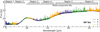 |
Fig. 1 Full JWST-MIRI spectrum (4.9–27.5 μm) of DR Tau. The different wavelength ranges (subbands) of each MIRI/MRS channel are shown in blue (‘A’), green (‘B’), and orange (‘C’), respectively. The wavelength regions over which H2O will be analysed are indicated by the horizontal bars. The continuum fit is indicated by the black line. |
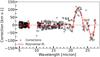 |
Fig. 2 Estimated wavelength corrections (black circles) for the selected lines. The red lines are the polynomials of degree 3 fitted for each JWST-MIRI subband and are used in correcting the wavelength calibration. |
3 Analysis and results
We analysed the H2O emission in DR Tau using four different methods: first, in Sect. 3.1, similar to Gasman et al. (2023), we investigated the H2O emission across separate regions in the spectrum using 0D local-thermal equilibrium (LTE) slab models (see Sect. 3.1). The slab model fitting procedure is described in detail in Temmink et al. (2024) (see also Grant et al. 2023 and Tabone et al. 2023). As the new reduction yields slightly different fluxes, especially in Channel 4, we report in Table A.1 new values for the median flux, the signal-to-noise ratio (S/N) as given by the JWST Exposure Time Calculator (ETC)1, which accounts for the degrading transmission2 of JWST-MIRI/MRS, and for the estimated noise on the continuum used in our fitting procedure. For the H2O slab models, we used grids where the column density (N in cm−2) was allowed to vary between 12 and 22 in log10-spacing using a of ΔN = 0.1. We note that these column densities probe the upper layers of the disk, above the height where the dust becomes optically thick, or, in the case of optically thick lines, above the height where the emission lines become optically thick (Bruderer et al. 2015; Woitke et al. 2018). The temperature (T) was allowed to vary between 150 and 2500 K in steps of ΔT = 25 K, whereas the emitting radius (Rem) was allowed to take on values between 0.01 and 10 au, using step sizes of ΔR = 0.024 au. The emitting radius is used as a parametrisation of the emitting area, assuming ![Mathematical equation: $\[A=\pi R_{\mathrm{em}}^2\]$](/articles/aa/full_html/2024/09/aa50355-24/aa50355-24-eq3.png) . We note that the emitting area does not have to be a circle, it can have any shape (i.e. an annulus) at any radial distance from the star. In addition to regions listed in Gasman et al. (2023) (5.0–6.5, 13.6–16.3, 17.0–23.0, and 23.0–27.0 μm), we also investigate the H2O emission in the regions between 7.0–9.5 and 10.5–13.0 μm. The different wavelength regions are also indicated in Fig. 1.
. We note that the emitting area does not have to be a circle, it can have any shape (i.e. an annulus) at any radial distance from the star. In addition to regions listed in Gasman et al. (2023) (5.0–6.5, 13.6–16.3, 17.0–23.0, and 23.0–27.0 μm), we also investigate the H2O emission in the regions between 7.0–9.5 and 10.5–13.0 μm. The different wavelength regions are also indicated in Fig. 1.
Second (see Sect. 3.2), we followed the method described in Banzatti et al. (2023a), where a continuum-subtracted spectrum of a large disk (CI Tau) was used to investigate a second, colder H2O component in a compact disk (GK Tau), after scaling for the differences in distances and luminosity of the H2O lines with highest upper energy levels (6000–8000 K). They expect this second component to trace the enrichment of the H2O gas near the snowline, following the sublimation of icy mantles of drifting grains. As DR Tau is a compact disk, we expect pebble drift to be efficient and, subsequently, we expect such a second H2O component should also be visible. Here, we also used the spectrum of CI Tau as the template spectrum to investigate the presence of an excess, cold second component in DR Tau (see Sect. 3.2.2). For consistency, the CI Tau observations have been reduced in the same way as done for DR Tau (see Sect. 2).
As a third method (Sect. 3.3), we investigate how well 0D LTE slab models can reproduce the observed spectrum when implementing radial and vertical temperature gradients.
Finally, we obtained limits on the H2O column density (in cm−2) by comparing the ratios of the Einstein-A coefficients and the line fluxes of H2O line pairs with the same upper energy level (Sec. 3.4, see also Gasman et al. 2023). We also searched for emission of the rare isotopologue H2 18O in Sec. 3.5, using the isolated lines listed in Calahan et al. (2022).
Additionally, in Sec. 3.6, we fitted an LTE slab model to the OH emission over the wavelength region between 10.0 and 27.5 μm and investigated the presence of other molecular species, such as CH4, NH3, and larger hydrocarbons. We compare their emission properties with those of H2O, CO2, HCN, and C2H2, of which the final three are presented in Temmink et al. (2024).
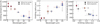 |
Fig. 3 Inferred gas temperature (left) and emitting radii (middle) for the different wavelength regions, and the emitting temperature as a function of the emitting radius (right). We show the results for the slab model fits without (squares) and with (circles) line overlap. The colours indicate the varying gas temperatures, whereas the horizontal bars denote the wavelength ranges of the regions. Errorbars are shown for the derived quantities, where those for the models without line overlap are shown in black and those for the models with line overlap are shown in red. In addition, we show for comparison the results (blacks stars) of the three component fit (approach 3, see Sect. 3.3.3) in the right panel. |
3.1 Single H2O LTE slab models
The JWST-MIRI observations of DR Tau show a plethora of both ro-vibrational (<10 μm) and rotational (>10 μm) transitions of H2O. Following Gasman et al. (2023), we investigated the excitation properties of H2O across different wavelength regions, covering both ro-vibrational and rotational transitions, using 0D-LTE slab models. We have used slab models without and with line overlap, i.e. mutual shielding of H2O lines (i.e. no shielding by other molecules, see Tabone et al. 2023 for a full description). Table 1 lists the best fitting slab model parameters for both the models without line overlap (top half) and with line overlap (bottom half). Figures displaying the best fitting slab models without and with line overlap are available online3.
The best fitting models were determined using a reduced χ2-minimisation method, following, for example, Grant et al. (2023), Tabone et al. (2023), and Temmink et al. (2024). The reduced χ2 is determined using the following equation:
![Mathematical equation: $\[\chi_{\text {red }}^2=\frac{1}{N_{\mathrm{obs}}} \sum_{i=1}^{N_{\mathrm{obs}}} \frac{\left(F_{\mathrm{obs}, i}-F_{\mathrm{mod}, i}\right)^2}{\sigma^2} .\]$](/articles/aa/full_html/2024/09/aa50355-24/aa50355-24-eq4.png) (1)
(1)
Here, Nobs is the number of spectral resolution elements, covering isolated H2O transitions, used in the fitting, Fobs and Fmod are the corresponding observed and model flux, respectively, and σ denotes the uncertainty on the flux (see Table A.1). The uncertainties on the best-fit parameters are taken from the confidence intervals, which are determined for, respectively, 1σ, 2σ, and 3σ as ![Mathematical equation: $\[\chi_{\text {red,min }}^2+2.3, ~\chi_{\text {red,min }}^2+6.2 \text { and } \chi_{\text {red.min }}^2+11.8\]$](/articles/aa/full_html/2024/09/aa50355-24/aa50355-24-eq5.png) (Avni 1976; Press et al. 1992).
(Avni 1976; Press et al. 1992).
In accordance with previous works (e.g. Blevins et al. 2016; Banzatti et al. 2023a; Gasman et al. 2023), the slab models probe the inner, hotter regions at the shortest wavelengths, whereas the outer, colder regions are traced by the longer wavelengths. The trends hold for both the models with and without line overlap. Figure 3 visualises the decreasing (increasing) trend of temperature (emitting radius) with wavelength for the models without overlap (squares) and those with line overlap (circles). We find that the temperatures decrease from 1000 K to 400 K over a span of 0.2 to 2.0 au, if Rem corresponds to the actual radius of the emitting area. Additionally, we show the temperature as a function of radius in the right panel of Fig. 3. This panel also includes the results from our three component fit (using method 3, see Sec. 3.3) and the 1σ uncertainties.
All fits yield generally well constrained values for the column densities, excitation temperatures and emitting areas, parameterised by the emitting radius Rem. The uncertainties, which are mostly within ±0.5 for the logarithm of the column density (in cm−2), ± 100 K for the excitation temperature, and ±0.20 au for the emitting radius, are the largest for the fits in region 6 (23.0–27.0 μm), likely the effect of this wavelength region having the lowest sensitivity. In addition, the upper uncertainty on the emitting radius for the third region is found to be higher compared to the other uncertainties. This is likely the result of this region having fewer bright, optically thick lines. Using the results for the inner two regions, those traced by the ro-vibrational H2O transitions, we can make a comparison with those for CO as analysed in Temmink et al. (2024), since those arise from a similar region of ~0.2 au. This comparison is made in Sec. 4.4.
We find that our slab models to the JWST-MIRI spectrum of DR Tau yield very similar results for the excitation temperatures and emitting radii for both the vibrational and rotational transitions of H2O compared to the previously mentioned ground-based, high spectral resolution observations (Najita et al. 2018; Salyk et al. 2019; Banzatti et al. 2023b). Furthermore, Banzatti et al. (2023b) provides linewidths for the vibrational H2O lines at 5.0 μm (FWHM ~ 22 km s−1) and the rotational transitions at 12.4 μm (FWHM ~ 16 km s−1), so we can estimate the emitting radii from these line profiles using Kepler’s law: R = GM* (sin(i)/Δυ)2, where i is the inclination of the disk (i ~ 5.4, as derived from ALMA observations; Long et al. 2019) and Δυ is the linewidth, here taken equal to half the width at half maximum (HWHM). We derive emitting radii of Rem ~0.06 au and ~0.11 au for the 5.0 and 12.4 μm high-resolution transitions, respectively. Both of these are significantly smaller than the derived emitting radii from our JWST observations and the slab models fitted to the ground-based, high-resolution observations. A similar discrepancy was found in our previous work, analysing the high spectral resolution CO observations (Temmink et al. 2024). There we found that the emitting radii derived from the slab models and those using the linewidths for CO agree if the (inner) disk inclinations are increased to iinner ~ 10–23°. Notably, observations of the VLTI-GRAVITY instrument suggest at similar inclinations for the inner disk (![Mathematical equation: $\[i_{\text {inner }} \sim 18_{-18}^{+10 \circ}\]$](/articles/aa/full_html/2024/09/aa50355-24/aa50355-24-eq43.png) ; GRAVITY Collaboration 2021). Using these inclinations, we derive emitting radii in the ranges of Rem ~ 0.21–0.96 au for vibrational transitions at 5 μm and Rem ~ 0.39–1.81 au, which do agree with the emitting radii derived from the slab models. As mentioned in Temmink et al. (2024), these derivations hold for the assumption that the emitting radii correspond to a circular region enclosing the host star and may suggest a misalignment between the inner and outer disk of DR Tau.
; GRAVITY Collaboration 2021). Using these inclinations, we derive emitting radii in the ranges of Rem ~ 0.21–0.96 au for vibrational transitions at 5 μm and Rem ~ 0.39–1.81 au, which do agree with the emitting radii derived from the slab models. As mentioned in Temmink et al. (2024), these derivations hold for the assumption that the emitting radii correspond to a circular region enclosing the host star and may suggest a misalignment between the inner and outer disk of DR Tau.
Best fit parameters of the H2O slab models without (top) and with line overlap (bottom).
3.2 Cold and warm H2O reservoirs: large disk template
3.2.1 Identifying unblended lines
Evidence for the presence of multiple rotational H2O components in the JWST-MIRI spectra was introduced by Banzatti et al. (2023a) and Gasman et al. (2023). In a similar fashion to Banzatti et al. (2023a), we first identified the unblended, high-energy (6000 ≤ Eup ≤ 8000 K) H2O lines, which all happen to have Einstein-A coefficients Aul > 10 s−1. Figures displaying Aul as a function of Eup (left panel) and wavelength (right panel) are available online4. As our analysis includes many more H2O lines compared to Banzatti et al. (2023a), we have identified fewer isolated lines. This is mainly due to the inclusion of transitions with low Einstein-A coefficients (<10−2 s−1). These low Einstein-A coefficient transitions are expected to have a negligible contribution to the spectrum, unless the transitions with high Einstein-A values have high optical depths of τ > 100.
To identify unblended, high-energy lines or high-energy lines that are blended together, we cross-listed these lines with all the transitions available (including Einstein-A coefficients <10−2 s−1) for the molecules detected in DR Tau. As mentioned above, the transitions with low Einstein-A coefficients may have a significant contribution to the spectra if the transitions with higher Einstein-A values have high optical depths. Consequently, we also considered using these transitions when identifying the unblended lines. In this process, we only included these lines in the wavelength regions in which molecules have been detected. For C2H2, CO2, and HCN this means that we cross-listed with all the available transitions in the region between 13.6 and 16.3 μm, whereas for OH we cross-listed with all transitions at wavelengths >13.6 μm. In addition, we cross-listed with all the low-energy (<6000 K) H2O transitions. If no transitions of any of the molecules are located within five resolution elements enclosing a high-energy H2O transition, we considered the transition to be useful for this analysis. Our cross-listing yielded a total of 24 potentially useful transitions, of which 11 are, upon visual inspection, strongly detected in both DR Tau and CI Tau. Of those 11 lines, six are blended together in three pairs and are, subsequently, treated as one.
3.2.2 Large disk template: CI Tau
We scaled the spectrum of CI Tau to match the flux level of the hot H2O transitions in DR Tau by accounting for the different distances and scaling by the averaged H2O line luminosity of the unblended lines of ![Mathematical equation: $\[L_{\mathrm{H}_2 \mathrm{O}, \text { DR Tau }} / L_{\mathrm{H}_2 \mathrm{O}, \mathrm{CI} \text { Tau }} \simeq 4.88\]$](/articles/aa/full_html/2024/09/aa50355-24/aa50355-24-eq44.png) . Figure 4 displays the (scaled) spectra of DR Tau (grey) and CI Tau (black) placed at a small flux offset with respect to the residuals in red over a large portion of the 10.0–27.5 μm wavelength region. Similar to Banzatti et al. (2023a), various cold H2O lines have excess flux present in the residuals, suggestive of a second, colder H2O emission component, likely the result of efficient radial drift. By fitting a simple LTE slab model to the residuals, which is also displayed in Fig. 4, we find that the second component has an excitation temperature of T = 375 K, traces a column density of N = 2.0 × 1019 cm−2, and has an emitting radius of Rem = 0.91 au.
. Figure 4 displays the (scaled) spectra of DR Tau (grey) and CI Tau (black) placed at a small flux offset with respect to the residuals in red over a large portion of the 10.0–27.5 μm wavelength region. Similar to Banzatti et al. (2023a), various cold H2O lines have excess flux present in the residuals, suggestive of a second, colder H2O emission component, likely the result of efficient radial drift. By fitting a simple LTE slab model to the residuals, which is also displayed in Fig. 4, we find that the second component has an excitation temperature of T = 375 K, traces a column density of N = 2.0 × 1019 cm−2, and has an emitting radius of Rem = 0.91 au.
Two lines just short of ~24 μm, indicated by the black, dashed rectangle in Fig. 4, are not well fitted by the residual slab model. These lines are also visible in the work of Banzatti et al. (2023a), who found that these are best fitted by an even colder component at T ~ 170 K, which most prominently emits at even larger wavelengths, ≥30 μm (Zhang et al. 2013; Blevins et al. 2016; Banzatti et al. 2023a).
3.3 Cold and warm H2O reservoirs: multi-component slab models
As shown in Sect. 3.2.2, the pure rotational H2O spectrum (≥10 μm) of DR Tau is best described by multiple, at least three, temperature components. In addition, following Sec. 3.1, the hotter (colder) components are thought to trace emission at shorter (longer) wavelengths with smaller (larger) emitting areas. A next step in the analysis of H2O would be to combine these notions: i.e., we fitted multiple slab models to the spectrum, consisting of components with decreasing temperatures and increasing emitting areas. The fitting is carried out using the Monte-Carlo Markov Chain implementation emcee (Foreman-Mackey et al. 2013), using 250 walkers and 150000 iterations. We test three different approaches for fitting multiple components, see also Fig. 5.
In the first approach (I) we assumed that the temperature only varies radially, accounting for the decreasing temperature gradient found in planet-forming disks. We consider that each component has a separate emitting region, with hotter components emitting from the smallest regions, closest to the host star. A simple radial temperature gradient is introduced by considering a weighted sum of the components, where the weights correspond to the emitting area (A), Ftotal=∑i FiAi. The flux of each component, Fi, is determined by a temperature Ti (in K) and a column density Ni (in cm−2), whereas the emitting area is parameterised by an emitting radius Ri (in au). For our three components, this yields the following total flux:
![Mathematical equation: $\[\begin{aligned}F_{\text {total }}= & F_1 \pi\left(\frac{R_1}{1 \mathrm{~au}}\right)^2+F_2 \pi\left[\left(\frac{R_2}{1 \mathrm{~au}}\right)^2-\left(\frac{R_1}{1 \mathrm{~au}}\right)^2\right] \\& +F_3 \pi\left[\left(\frac{R_3}{1 \mathrm{~au}}\right)^2-\left(\frac{R_2}{1 \mathrm{~au}}\right)^2\right].\end{aligned}\]$](/articles/aa/full_html/2024/09/aa50355-24/aa50355-24-eq45.png) (2)
(2)
As planet-forming disks also have a vertical temperature gradient, we allowed the colder components in the second approach (II) to also emit from the overlapping regions with the hotter components. If we are not taking shielding into account and assume that the various components have overlapping emitting areas, the total flux simply becomes:
![Mathematical equation: $\[F_{\text {total }}=F_1 \pi\left(\frac{R_1}{1 \mathrm{~au}}\right)^2+F_2 \pi\left(\frac{R_2}{1 \mathrm{~au}}\right)^2+F_3 \pi\left(\frac{R_3}{1 \mathrm{~au}}\right)^2.\]$](/articles/aa/full_html/2024/09/aa50355-24/aa50355-24-eq46.png) (3)
(3)
In the final approach (III), we accounted for shielding of the colder, deeper components by the optical depth of the hotter components. In the case of shielding, the flux is attenuated by a factor of exp (− ∑iτi), where the sum is taken over the optical depths of all the components with a higher temperature. The optical depth is taken to be wavelength-dependent determined for all transitions combined using the corresponding excitation temperature and column density. As shown in Sects. 3.1 and 4.1, and in Table 1, the mutual line shielding by neighbouring H2O transitions does not have a significant impact on the slab models and, hence, we only account for the spatial shielding of colder components by the hotter ones (see Fig. 5). The total flux of the this approach, in which we account for spatial line shielding of the colder components by the hotter one, becomes:
![Mathematical equation: $\[\begin{aligned}F_{\text {total }}= & F_1 \pi\left(\frac{R_1}{1 \mathrm{~au}}\right)^2+F_2 \pi\left(\frac{R_1}{1 \mathrm{~au}}\right)^2 \exp \left(-\tau_1\right) \\& +F_2 \pi\left[\left(\frac{R_2}{1 \mathrm{~au}}\right)^2-\left(\frac{R_1}{1 \mathrm{~au}}\right)^2\right]+F_3 \pi\left(\frac{R_1}{1 \mathrm{~au}}\right)^2 \exp \left(-\left(\tau_1+\tau_2\right)\right) \\& +F_3 \pi\left[\left(\frac{R_2}{1 \mathrm{~au}}\right)^2-\left(\frac{R_1}{1 \mathrm{~au}}\right)^2\right] \exp \left(-\tau_2\right) \\& +F_3 \pi\left[\left(\frac{R_3}{1 \mathrm{~au}}\right)^2-\left(\frac{R_2}{1 \mathrm{~au}}\right)^2\right]\end{aligned}\]$](/articles/aa/full_html/2024/09/aa50355-24/aa50355-24-eq47.png) (4)
(4)
For the two component version, all terms including F3 can be neglected.
For all three approaches, we considered three components and imposed the following constraints: the temperature must decrease with each component, whereas the emitting radius must increase. We kept the column density as a completely free parameter. In addition, we also show a model with two components for the third method, which allows for a thorough comparison between the models. The results for the different approaches are presented in the following subsections.
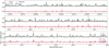 |
Fig. 4 Spectra (across 13.4–24.0 μm) of DR Tau (grey) and CI Tau (black, scaled; see Sect. 3.2.2) shown together with the residual spectrum (in red) of DR Tau after subtraction of the scaled spectrum of CI Tau. The best fitting H2O slab model (T = 375 K) to the residuals is shown in blue. The black dashed box just shortward of ~24.0 μm indicates the pair of lines identified by Banzatti et al. (2023a), hinting at a third component (~170 K) needed to fully explain the observed H2O reservoir. |
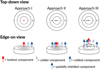 |
Fig. 5 Cartoon visualising the different radial and vertical temperature gradients tested in this work. A top down version is shown in the top half of the figure, whereas as an edge-on view is shown in the bottom half. The coloured arrows indicate the emission from the different components, with red showing the emission from the hottest component, light blue for the component with the intermediate temperature, and dark blue for the coldest component. The dashed arrows indicate emission originating from spatially shielded regions. |
Best-fit parameters for the multiple component slab model fits, including radial and vertical temperature gradients.
3.3.1 Radial temperature gradient
The top part of Table 2 contains median values yielded by the MCMC for the first approach. The uncertainties are given, respectively, by the 16th and 84th percentiles. For this first approach, we retrieve temperatures of ![Mathematical equation: $\[806_{-154}^{+289}\]$](/articles/aa/full_html/2024/09/aa50355-24/aa50355-24-eq80.png) K,
K, ![Mathematical equation: $\[468_{85}^{+79}\]$](/articles/aa/full_html/2024/09/aa50355-24/aa50355-24-eq81.png) K, and
K, and ![Mathematical equation: $\[181_{-43}^{+36}\]$](/articles/aa/full_html/2024/09/aa50355-24/aa50355-24-eq82.png) K for the different components. In addition, we obtain combinations for the column density (log10 (N), with N in units of cm−2) and emitting radius of, respectively,
K for the different components. In addition, we obtain combinations for the column density (log10 (N), with N in units of cm−2) and emitting radius of, respectively, ![Mathematical equation: $\[19.2_{-0.5}^{+1.5}\]$](/articles/aa/full_html/2024/09/aa50355-24/aa50355-24-eq83.png) and 0.35±0.15 au,
and 0.35±0.15 au, ![Mathematical equation: $\[18.5_{-0.4}^{+0.9}\]$](/articles/aa/full_html/2024/09/aa50355-24/aa50355-24-eq84.png) and
and ![Mathematical equation: $\[1.18_{-0.18}^{+0.27}\]$](/articles/aa/full_html/2024/09/aa50355-24/aa50355-24-eq85.png) au, and
au, and ![Mathematical equation: $\[17.9_{-0.7}^{+2.2}\]$](/articles/aa/full_html/2024/09/aa50355-24/aa50355-24-eq86.png) and
and ![Mathematical equation: $\[6.45_{-2.64}^{+2.26}\]$](/articles/aa/full_html/2024/09/aa50355-24/aa50355-24-eq87.png) au. The best fitting model is displayed in the top panel of Fig. 6. The corner plots are available online5.
au. The best fitting model is displayed in the top panel of Fig. 6. The corner plots are available online5.
3.3.2 Radial and vertical temperature gradient: no shielding
The resulting values for the second approach are shown in the second part of Table 2. Compared with approach I, assuming only a radial gradient with no spatial overlap, our best fit parameters do not significantly change. In particular, the main difference can be found in the emitting radius of the third, coldest component. However, the values still agree within the given uncertainties and show a clear gradient. The final model is shown in the middle panel of Fig. 6. The corresponding corner plots are available online6.
3.3.3 Radial and vertical temperature gradient: accounting for spatial shielding
The results for the three component and two component fits, using the third approach, are shown in respectively the third and bottom parts of Table 2. For the three component fit (also visible in the bottom panel of Fig. 6), we find that the best fit parameters are similar to those of the second approach. That means that the main difference can once more be found in the emitting radius of the third component. It must be noted that the values for all three approaches agree with one another within the given uncertainties. In accordance with Pontoppidan et al. (2024), we find that the results for this approach can be well described by the power-law ![Mathematical equation: $\[T\left(R_{\mathrm{em}}\right) \sim 500\left(\frac{R_{\mathrm{em}}}{1 \mathrm{~au}}\right)^{-0.5}\]$](/articles/aa/full_html/2024/09/aa50355-24/aa50355-24-eq88.png) K for the emitting layer. For the two component fit, we see that the temperature of the first (hottest) component and the second component are lower by ≳ 100 K. It is clear that the coldest component, T ~ 180 K, is not considered by the two component fit. A figure displaying the two component fit is available online7. The column density and the emitting radius of the first component have, respectively, slightly decreased and increased with respect to the three component fit. On the other hand, only the emitting radius of the second component increased from ~1.20 au to ~1.83 au. The corner plots for the three and two components fits are available online8.
K for the emitting layer. For the two component fit, we see that the temperature of the first (hottest) component and the second component are lower by ≳ 100 K. It is clear that the coldest component, T ~ 180 K, is not considered by the two component fit. A figure displaying the two component fit is available online7. The column density and the emitting radius of the first component have, respectively, slightly decreased and increased with respect to the three component fit. On the other hand, only the emitting radius of the second component increased from ~1.20 au to ~1.83 au. The corner plots for the three and two components fits are available online8.
We find that all models underproduce the flux for a range of H2O transitions between ~14 μm and ~18 μm. This region is dominated by both the first (hottest) and second (warm) component, suggesting that either one or both components do not properly describe this region and slightly different values for the parameters would yield a better fit. Nonetheless, the fit provides an overall good description of the observed rotational spectrum of H2O in DR Tau.
Finally, Fig. 7 displays an cartoon of the disk, indicating the expected emission locations from our multi-component fit. We have also included the expected locations from CO, CO2, HCN, C2H2 as found in Temmink et al. (2024) (see also their Fig. 12), based on their excitation temperatures and emitting areas.
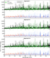 |
Fig. 6 Multi-component slab model fits for the different methods of radial gradients: method 1 (radial temperature gradient, without overlapping regions) is shown in the top panel, whereas the methods 2 (radial gradients with overlapping regions, but no line shielding) and 3 (radial and vertical temperature gradients) are displayed in the middle and bottom panels, respectively. The full model is in each panel shown in green, whereas the components are coloured depending on the corresponding temperatures. Red indicates the hottest component, followed by the light blue and dark blue ones. The green horizontal bars indicate the regions used in the |
![Mathematical equation: $\[\chi_{\text {red }}^2\]$](/articles/aa/full_html/2024/09/aa50355-24/aa50355-24-eq89.png)
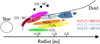 |
Fig. 7 Cartoon visualising the expected emission regions, based on the derived excitation temperatures, emitting radii, and optical depths, of the multiple components of H2O. Shown are also the expected emission locations of CO, CO2, HCN, and C2H2 adopted from Temmink et al. (2024). The CO is decomposed in two components: one broad component (BC) tracing the Keplerian rotation of the disk, and a narrow component (NC) tracing a disk wind. |
3.4 Line pair ratios
The inferred column density of the slab models can be tested and further constrained by comparing the peak fluxes of H2O line pairs which have the same value for Eup, but different values for Aul (Gasman et al. 2023). As the strength of these lines and, therefore, their ratio depends primarily on the line opacity, they can be used to approximate as independent constraints on the column density and provide a sanity check for the column densities retrieved with the slab models. If both lines are optically thin, the flux ratio is expected to converge to the ratio of the respective values for Aul, whereas the flux ratio will deviate from the Aul ratio if one of the lines becomes optically thick. We use the same, pure rotational line pairs as Gasman et al. (2023) (see their Table 2) to investigate the H2O column density. Some of the lines are part of line clusters and are, subsequently, blended, which means that it cannot be concluded from the flux ratio alone which of the lines are optically thick, if the flux ratio deviates from that of Aul.
Figure 8 shows the model line ratios for different temperatures (300, 500, and 900 K) and column densities (14 ≤ log10(N) ≤ 22, with N in units of cm−2). The ratios become constant for column densities of ≤1017 cm−2. For these column densities we can expect both lines to be optically thin and, subsequently, their ratios to be equal to the values for Aul. At larger column densities (at least) one of the lines becomes optically thick and the ratio deviates from that for Aul. For even larger column densities (≥1020 cm−2) the ratio becomes constant again, the effect of both lines being fully saturated.
The black horizontal line shown in Fig. 8 is the line ratio obtained from the JWST-MIRI spectrum. The coloured, dotted vertical lines are the intercepts between the black horizontal line and the model ratio curves. Based on the intercept, we can expect the actual H2O column density to take on values of ≤1019.4 cm−2, ≤1018.4 cm−2, and/or ≤1018.0 cm−2 for the different temperatures (T = 300, 500, and 900 K), respectively. Using the results from the multi-component fits, we can infer the contributions from each component to the lines used for both line pairs. For the bottom pair (115.6−104,7/115,6−102,9), both transitions consist of contributions from the hotter two components, so the T ~ 300 K models can be ignored. For both transitions, the lower temperature (T ~ 475 K) has a slightly larger contribution to the flux. Based on this line pair and the temperature from both contributing components (T ~ 830 K and T ~ 475 K), we infer that the column density of the combination of these two H2O components must be log10 (N) ≤ 18.5 within ~1.2 au. For the top pair (87,2−74,3/87,2−76,1), however, the lowest temperature component (T ~ 185 K) also has a significant contribution to the line flux of one of the lines. As only one of these lines has a contribution from the lowest temperature component, this pair does not provide strong constraints. After subtracting off the model corresponding to this temperature, we do infer a slightly more stringent constraint on the H2O column density (in cm−2) of log10 (N) ≤ 18.4 for the first two components combined, compared to value derived for the other line pair. Even though H2O is optically thick, these line pair ratios provide good constraints on the column densities for the first two components. We note that the derived limit agrees well with those obtained for the second, warm component, whereas it falls just outside the uncertainties for the hottest, most optically thick component.
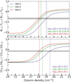 |
Fig. 8 Logarithm of the line flux ratios as a function of the logarithm of the column densities (in cm−2) for the line pairs with similar upper level energies. The ratios for the slab models with T =300 K are shown in blue, whereas those for T = 500 K and T = 900 are shown in green and red, respectively. The horizontal black line indicates the line ratio taken from the continuum-subtracted spectrum of DR Tau. The dashed, vertical lines indicate where the different model ratios equal the observed line ratio. In addition, the dotted lines and the column densities listed in parenthesis indicate the results for the top line pair after subtracting off the contribution of the component with the lowest temperature (see Sect. 3.3). |
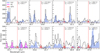 |
Fig. 9 Zoom-ins on the isolated H2 18O lines, highlighted by the red vertical line. A simple H2 18O slab model (T = 350 K, log10 (N) = 17.66, and Rem = 1.0 au) is shown in red, whereas the best models of H2O (three component fit accounting for both the radial and vertical temperature gradient) and OH are shown in blue and magenta, respectively. For each transition, we have listed the upper level energies and Einstein-A coefficients. |
3.5 Searching for H2 18O
We are inconclusive about the detection of H2 18O in DR Tau. Some of the transitions, in particular those at 25.65, 26.83, and 26.99 μm, look promising (see Fig. 9). Accounting for the large error in subband 4C (see Table A.1), the peak fluxes suggest maximum detection levels of ≲4σ and should be statistically significant for the confirmation of a detection. However, the lack of flux seen for the transitions at ~22.03 μm and ~23.17 μm provide the strongest argument against a detection of H2 18O in DR Tau. Re-observing DR Tau with JWST-MIRI with the aim of achieving higher signal-to-noise ratios across Channel 4 may improve our chances of detecting H2 18O.
Using our three component models, we find that the majority of the H2O emission features are optically thick. While transitions with low Einstein-A values may be optically thin and can be used to derive better constraints on the total H2O vapour reservoir present in the inner disk, we note that these lines are very scarce in the spectrum of DR Tau. In total, we identify four clean emission features (between 12.496–12.506, 14.377–14.392, 16.362–16.375, and 19.370–19.392 μm) that are optically thin (τ <1) according to our models and not blended with other (unidentified) emission features. All these transitions trace mainly the hottest component. Subsequently, a fit to these transitions only may provide a better constraint on the column density for the hottest component and observations of the optically thin isotopologues, such as H2 18O, could help to infer a better estimate of the column density and the total number of H2O molecules present in the inner disk.
Calahan et al. (2022) list eight lines in the 19.0–27.0 μm wavelength range that may be used for the detection of H2 18O in JWST-MIRI spectra (see their Table 1). We, however, note that the line at 20.01 μm is blended with OH and can likely not be used for the detection of H2 18O in many T-Tauri disks. On the other hand, through slab model exploration we discovered a blended pair of H2 18O lines that can be used instead. The line pair (88,0−77,1 and 88,1−77,0) is located at 25.65 μm and have the same upper level energies (Eup ~2544.9 K) and Einstein-A coefficients (Aul ~29.08 s−1), suggesting that both lines contribute half of the observed line flux. The individual lines are displayed in Fig. 9. The H2 18O emission is highlighted by a simple H2 18O slab model (T = 350 K, log10 (N) = 17.36, and Rem = 1.0 au), where we have accounted for the isotopologue ratio in the local interstellar medium (ISM) of 16O/18O~550 (Wilson 1999) in the column density, i.e. we have divided the found column density of H2O in the wavelength region of 23.0–27.0 μm (log (N) ~ 20.1, see Table 1) by 550. We show our best fitting H2 16O and OH slab models (see Table 1 and Sect. 3.6.1) for further identification. A figure displaying the full 17.0–27.5 μm wavelength region, including the aforementioned H2 16O, H2 18O, and OH slab models, is available online9.
Even though we are inconclusive about the detection of H2 18O, the used slab model yields underproduced fluxes for the most promising peaks. This may suggest that, for the used temperature, the input column density is not high enough. As the column density was set to account for the isotopologue ratio (16O/18O~550), this indicates optically thick H2O emission, which is in agreement with our models. We note that an underestimate of the column density for H2 18O may also point to a deviation of the isotopologue from the ISM value. As discussed in Calahan et al. (2022), the gas may be enriched in H2 18O in the disk layers where CO becomes optically thick and self-shielding against photodissociation becomes important. As the main isotopologue, C16O, is more abundant than C18O, there will be a layer where C16O will be self-shielded, whereas C18O is still being dissociated. The gas in this layer will in that case be enriched in 18O atoms, which may end up in H2O-molecules, enhancing the H2 18O column. Additionally, UV-shielding by the main isotopologue, H2 16O, can also enhance the H2 18O abundance.
3.6 Other emission features
Besides emission from H2O, the spectrum of DR Tau is rather molecule rich. CO, CO2, HCN, and C2H2 have been thoroughly discussed been in Temmink et al. (2024), so the upcoming subsections discuss the other molecular features potentially present in the spectrum, including OH and the larger hydrocarbons that have been observed in the disks around very low-mass stars (e.g. Tabone et al. 2023).
3.6.1 OH
Since we do not detect any OH lines at wavelengths <13 μm, similar to Gasman et al. (2023), we do not expect prompt emission, following H2O photodissociation (Najita et al. 2010), to play a role in the observed OH emission in DR Tau. We fit the OH emission, using a reduced χ2-minimisation (see also Sect. 3.1), over the entire wavelength range of 10 μm to 27.5 μm. We have used the same grid for T, log10 (N), and Rem as in Sect. 3, except we extended the grid for the excitation temperature up to 4000 K. The emission was fit to the residual spectrum after subtracting the resulting H2O model spectrum taking both a radial and vertical temperature gradient into account (see Sect. 3.3.3). For OH, we retrieve a temperature of ![Mathematical equation: $\[T{=}1875_{-725}^{+775}\]$](/articles/aa/full_html/2024/09/aa50355-24/aa50355-24-eq90.png) K, a column density (in cm−2) of
K, a column density (in cm−2) of ![Mathematical equation: $\[\log ~(N){=}13.5_{-0.3}^{+3.3}\]$](/articles/aa/full_html/2024/09/aa50355-24/aa50355-24-eq91.png) , and emitting radius of
, and emitting radius of ![Mathematical equation: $\[R_{\mathrm{em}}{=}9.49_{-9.06}^{+0.52}\]$](/articles/aa/full_html/2024/09/aa50355-24/aa50355-24-eq92.png) au. As the emission is optically thin (τ ≤ 0.005) for this combination of excitation temperature and column density, the emitting radius is not well constrained, as indicated by the large lower uncertainty. We note that the upper uncertainty of the emitting radius and, therefore, the lower constraints on the column density are set by the limits of our grids. For these parameters, we derive that the number of OH molecules present in the inner disk of DR Tau is
au. As the emission is optically thin (τ ≤ 0.005) for this combination of excitation temperature and column density, the emitting radius is not well constrained, as indicated by the large lower uncertainty. We note that the upper uncertainty of the emitting radius and, therefore, the lower constraints on the column density are set by the limits of our grids. For these parameters, we derive that the number of OH molecules present in the inner disk of DR Tau is ![Mathematical equation: $\[\mathcal{N}\]$](/articles/aa/full_html/2024/09/aa50355-24/aa50355-24-eq93.png) ~ 2.0 × 1042. Figures displaying parts of the best fitting model, including the wavelength regions used in the fitting, are available online10. Similar to Gasman et al. (2023), the OH lines probe larger gas temperatures compared to H2O, but lower column densities. As the excitation of the OH lines includes prompt emission (Tabone et al. 2021, 2024) and collisional excitation or chemical pumping (Zannese et al. 2024) through the O+H2→OH+H reaction, it is unlikely that the observed transitions follow a single excitation temperature. Therefore, the inferred temperature from the slab model is not related to a kinetic temperature. While they cannot infer a kinetic temperature, we note that slab models are a powerful tool for the identification of OH transitions in the JWST-MIRI/MRS spectra of disks. Detailed models, including the different excitation pathways, can be used to further explore the excitation properties and to infer other key disk parameters (see, for example, Tabone et al. 2024).
~ 2.0 × 1042. Figures displaying parts of the best fitting model, including the wavelength regions used in the fitting, are available online10. Similar to Gasman et al. (2023), the OH lines probe larger gas temperatures compared to H2O, but lower column densities. As the excitation of the OH lines includes prompt emission (Tabone et al. 2021, 2024) and collisional excitation or chemical pumping (Zannese et al. 2024) through the O+H2→OH+H reaction, it is unlikely that the observed transitions follow a single excitation temperature. Therefore, the inferred temperature from the slab model is not related to a kinetic temperature. While they cannot infer a kinetic temperature, we note that slab models are a powerful tool for the identification of OH transitions in the JWST-MIRI/MRS spectra of disks. Detailed models, including the different excitation pathways, can be used to further explore the excitation properties and to infer other key disk parameters (see, for example, Tabone et al. 2024).
3.6.2 Atomic and molecular hydrogen
We list the detection of three atomic hydrogen (H) transitions (10–6, 6–5, and 8–6) and the potential detection of four molecular hydrogen (H2) transitions: 0,0 S(1), S(2), S(3), and S(4). As the H2 lines are either blended with H2O or potentially blended with unidentified features, their detections are not fully secure. Higher transitions (e.g. S(5), S(6), S(7), and S(8)) may also be present, however, their detections are even less certain due to stronger blending with H2O and CO emission features. Figures displaying the (potentially) observed transitions of H and H2 (S(1), S(2), S(3), and S(4)) are available online11. We also see no evidence of extended H2 emission coming from the DR Tau disk in the form of a disk wind or an outflow, however, we do observe extended H2 emission (most prominent in the S(1) transition) from the cloud surrounding DR Tau, as was previously observed by Thi et al. (2001) in millimetre single dish CO J = 3–2 transitions offset by ~2 km s−1. A figure visualising the background emission is available online12. Visual inspection of the spectral cube shows that the flux of the cloud emission (FS(1) ~ 2 × 10² MJy sr−1) is a factor ~100 lower than the flux at the position of DR Tau (FS(1) ~ 2 × 10⁴ MJy sr−1). As we approximate our background using an annulus, the H2 emission from the cloud will be captured in that annulus. However, as the flux is significantly lower than the source flux, the background subtraction does not impact our detections.
Using the residual flux, after subtracting the corresponding H2O slab model fit, we determined an upper limit on the column density of H2 based on the 0,0 S(4) transition (Eup = 3474.5 K). Assuming that H2 comes from the inner most region, we adopt a temperature of T = 1000 K and an emitting radius of Rem = 0.20 au, as this also allows us to make direct comparisons with the total number of molecules of both CO and H2O (as obtained in regions 1 and 2 for the ro-vibrational transitions, see Sec. 3.1) derived in these innermost regions. To calculate the column density under the assumption of optically thin emission, we follow the description given in Goldsmith & Langer (1999):
![Mathematical equation: $\[\frac{4 \pi F}{h c \nu \Omega g_{\mathrm{up}} A_{\mathrm{ul}}}=\frac{N_{\mathrm{tot}}}{Q(T)} \exp \left(-\frac{E_{\mathrm{up}}}{k_B T}\right),\]$](/articles/aa/full_html/2024/09/aa50355-24/aa50355-24-eq94.png) (5)
(5)
where F is the integrated flux (in erg s−1 cm−2), ν the frequency (in cm−1), gup the upper level degeneracy, Q(T) the partition function at a temperature T, and Eup the upper level energy (in K). Using the resolution element at the location of the S(4) transition and the two resolution elements directly next to it, we derive F=3.9×10⁻¹⁵ erg s−1 cm−2. As mentioned above, the H2 flux might be slightly affected by the annulus background subtraction due to cloud emission. However, as the background emission is significantly lower than the on-source emission, we expect the derived flux to be minimally impacted. This yields a column density of Ntot ~ 7.6 × 1025 cm−2 and a total number of molecules, assuming an emitting radius of 0.20 au, of ![Mathematical equation: $\[\mathcal{N}_{\mathrm{H}_2} \sim 2.1 {\times} 10^{51}\]$](/articles/aa/full_html/2024/09/aa50355-24/aa50355-24-eq95.png) . We note once more that these derived column densities and total number of molecules hold for the upper layers of the disk, above the region where the dust emission becomes optically thick, or, in the case of optically thick lines, above the height where the emission lines become optically thick (see, for example, Bosman et al. 2022).
. We note once more that these derived column densities and total number of molecules hold for the upper layers of the disk, above the region where the dust emission becomes optically thick, or, in the case of optically thick lines, above the height where the emission lines become optically thick (see, for example, Bosman et al. 2022).
3.6.3 Non-detections
In an attempt to identify as many molecular features as possible, we have also looked for emission signatures of various other molecules and isotopologues. These species are comprised of 13CO2, CH4, NH3, CS, H2S, SO2, and various larger hydrocarbons, including 13CCH2. We have obtained the required spectroscopic data for these species through the HITRAN database (Gordon et al. 2022). Table 3 summarises the parameters (assuming an emitting radius of Rem = 1.0 au) of simple LTE slab models with fixed temperature and column density that have been used to search for these species. In addition, the table lists the best fit parameters for CO2, HCN, and C2H2, as found in Temmink et al. (2024). Figures displaying the slab models are available online13.
We are not able to confidently detect any of the listed molecular species. The non-detection of some the molecules, for example, 13CO2, CH4, SO2, and the larger hydrocarbons, becomes apparent from the slab models, mostly due to the lack of a molecular continuum. For the other molecules, NH3, CS, H2S, and 13CCH2, a (non-)detection cannot be confirmed, largely due to leftover broad features (especially visible at the location of the silicate feature at ~10 μm), which are potentially of molecular nature, in the spectrum. We also do not detect the larger hydrocarbons, mostly due to the lack of molecular continua. While the slab model14 of C6H6 looks promising, the presence of C6H6 cannot be confirmed in the spectrum of DR Tau, as the lack of emission observed for the other hydrocarbons makes the presence of C6H6 less likely.
For most of the non-detected molecules, the upper limit on the total number of molecules is on the order of ![Mathematical equation: $\[\mathcal{N}\]$](/articles/aa/full_html/2024/09/aa50355-24/aa50355-24-eq96.png) ~1042−1043. Only the upper limit for H2S is larger (
~1042−1043. Only the upper limit for H2S is larger (![Mathematical equation: $\[\mathcal{N}\]$](/articles/aa/full_html/2024/09/aa50355-24/aa50355-24-eq97.png) ~ 7.0×1044), whereas that for C6H6 is significantly lower (
~ 7.0×1044), whereas that for C6H6 is significantly lower (![Mathematical equation: $\[\mathcal{N}\]$](/articles/aa/full_html/2024/09/aa50355-24/aa50355-24-eq98.png) ~ 1.3×1038). Using the number of molecules from our three component H2O fits (
~ 1.3×1038). Using the number of molecules from our three component H2O fits (![Mathematical equation: $\[\mathcal{N}\]$](/articles/aa/full_html/2024/09/aa50355-24/aa50355-24-eq99.png) ~ 1045−1046), most of the non-detected molecules are a factor ≥102−104 less abundant than H2O. H2S and C6H6 are factors of, respectively, ≥10–100 and ≥107−108 less abundant. On the other hand, the upper limits are of a similar level compared to the total number of molecules derived for CO2, HCN, and C2H2. Once again, the upper limit for H2S is slightly larger, whereas that of C6H6 is a few orders of magnitude lower. For comparison, the abundance of CO2 is found to be a factor ~60 lower than the second, warm component of H2O.
~ 1045−1046), most of the non-detected molecules are a factor ≥102−104 less abundant than H2O. H2S and C6H6 are factors of, respectively, ≥10–100 and ≥107−108 less abundant. On the other hand, the upper limits are of a similar level compared to the total number of molecules derived for CO2, HCN, and C2H2. Once again, the upper limit for H2S is slightly larger, whereas that of C6H6 is a few orders of magnitude lower. For comparison, the abundance of CO2 is found to be a factor ~60 lower than the second, warm component of H2O.
Slab models parameters of the various detected (CO2, HCN, C2H2; Temmink et al. 2024) and non-detected species, using Rem=1 au.
4 Discussion
4.1 The need for H2O line overlap
For slab model fits of molecules with a well defined Q-branch (see Tabone et al. 2023), line overlap (i.e. mutual shielding of lines) is often included to properly fit the spectra. The spectrum of H2O, on the other hand, consists of well defined, separate/isolated transitions. In the disk of AS 209, Muñoz-Romero et al. (2024) also tested the need for line overlap of multiple molecular species. They conclude that a proper treatment of the line overlap is necessary when analysing the observed molecular species together.
In Sec. 3.1, we test the need for mutual shielding by the H2O transitions alone. We test this by creating slab models without and with mutual line shielding. As can be seen in Table 1, the differences between the slab models without (top part of the table) and those with (bottom part) mutual line overlap are negligible when fitting H2O alone. The largest differences are found for temperatures derived for the regions spanning the ro-vibrational transitions, which is likely due to the lines being more densely packed in this part of the spectrum compared to those in the pure rotational part. We note that the residuals for the models without and with mutual line shielding are quite similar. We find that one model will provide a better fit for some transitions, whereas other transitions are better fitted by the other model. Therefore, we conclude that the inclusion of mutual shielding of neighbouring H2O lines is not of particular importance for the pure rotational transitions of H2O, when fitting them alone, and that the slab models without mutual line shielding can be used to infer constraints on the excitation conditions. As our slab models yield different results for the rovibrational part of the spectrum, the inclusion of mutual shielding may be more important for these more densely packed transitions. Mutual line shielding is of particular importance for molecules with a well defined Q-branch, such as CO2, HCN, and C2H2.
4.2 The need for a radial temperature gradient
As expected, the various methods all indicate a radial temperature gradient visible in the spectrum. Fitting, however, the H2O spectrum across multiple, independent wavelength regions does not yield any information on the low temperature (T ~ 170–200 K, see Table 1) component, even though the fitted regions include the lines best suitable for finding this component. Subsequently, to properly investigate the various components, one could use the large disk template method implemented by Banzatti et al. (2023a) or the multi-component slab model method introduced here.
Rather surprisingly, the current approaches of the multi-component slab model fits yield the same results for all three methods: temperatures of ~800 K, ~470 K, and ~180 K, column densities of ~1019.2 cm−2, ~1018.5 cm−2, and ~1017.4 cm−2, and emitting radii of ~0.3 au, ~1.2 au, and ~6.5–8.1 au. For comparison, the midplane H2O snowline in DR Tau can be estimated from a simple power law (Chiang & Goldreich 1997; Dullemond et al. 2001; van der Marel et al. 2021) involving the total luminosity (Ltot=L* +Lacc ≃0.63 + 0.58 L⊙; Long et al. 2019; Banzatti et al. 2020), providing a radius ![Mathematical equation: $\[R_{\mathrm{H}_2 \mathrm{O}} \sim 0.75\]$](/articles/aa/full_html/2024/09/aa50355-24/aa50355-24-eq107.png) au. The calculations of Mulders et al. (2015) (see their Fig. 1) suggest that the snowline is located at a radial distance of ~1–2 au. Radiative transfer modelling of the dust disks may provide further constraints on the location of the H2O snowline. As the third component at ~180 K is at larger distances than the midplane snow surface, this suggests a curved rather than vertical snow surface. We find that the decreasing temperature profile can be well described by the powerlaw
au. The calculations of Mulders et al. (2015) (see their Fig. 1) suggest that the snowline is located at a radial distance of ~1–2 au. Radiative transfer modelling of the dust disks may provide further constraints on the location of the H2O snowline. As the third component at ~180 K is at larger distances than the midplane snow surface, this suggests a curved rather than vertical snow surface. We find that the decreasing temperature profile can be well described by the powerlaw ![Mathematical equation: $\[T\left(R_{\mathrm{em}}\right) \sim 500\left(\frac{R_{\mathrm{em}}}{1 \mathrm{~au}}\right)^{-0.5} \mathrm{~K}\]$](/articles/aa/full_html/2024/09/aa50355-24/aa50355-24-eq108.png) K. Only the emitting radius for the final component differs between approach 1 and approaches 2 and 3, but still agrees well within the given uncertainties. The resulting temperatures agree with those given by the large scale template method, in particular the third component (T ~ 180 K) corresponds well with the one (T ~ 170 K) that Banzatti et al. (2023a) needed to explain the lines just shortward of 24 μm. To extend upon this notion, a figure showing a comparison between the multi-component fits including three and two components is available online15. The main difference is most clearly visible in the region of 23.50–24.25 μm, which includes the aforementioned cold lines. The two component model is not able to properly fit this line cluster, whereas the three component model can.
K. Only the emitting radius for the final component differs between approach 1 and approaches 2 and 3, but still agrees well within the given uncertainties. The resulting temperatures agree with those given by the large scale template method, in particular the third component (T ~ 180 K) corresponds well with the one (T ~ 170 K) that Banzatti et al. (2023a) needed to explain the lines just shortward of 24 μm. To extend upon this notion, a figure showing a comparison between the multi-component fits including three and two components is available online15. The main difference is most clearly visible in the region of 23.50–24.25 μm, which includes the aforementioned cold lines. The two component model is not able to properly fit this line cluster, whereas the three component model can.
Compared to results from fitting H2O across the different wavelength regions (see Sec. 3.1), we note that the derived column densities for these methods do not show the same behaviour. For the multi-component fit, the column densities decrease with lower temperatures, whereas they increase with temperature for the different regions. The difference in behaviour may have arisen from combining the contribution of every component in the multi-component fits, whereas contributions of other components and/or wavelength regions have not been accounted for in the fits to the different wavelength regions.
A multi-component fit could, instead of a large disk model, also be used to investigate the enhanced reservoir of cold H2O through radial drift. We expect that a two component fit is sufficient to fit the spectra without enhancement of cold H2O through radial drift, whereas three component fits are required to properly fit those with the enhancement. Further work examining a large sample of disks, small and large, structured and smooth, is necessary to fully explore this thought.
The reason why all three models yield the same results is due to line optical depths. These optical depths are too high (reaching values up to τ ~ 3000 for the innermost region and τ ~ 350 for the first annulus for the brightest lines) for any of the shielded regions to make a significant contribution to the total model. In other words, considering only the innermost region, the optical depth of the hottest components is so high that the contributions (i.e. those with an exponential in Eq. (4)) of the lower temperature components are negligible. As discussed in Sec. 3.4, the column density (in cm−2) of the warmer two components (components 1 and 2) can be expected to be on the order of log (N) ~ 18.4.
When using simple LTE slab models to describe the full rotational spectrum of H2O, it is clear that a vertical temperature gradient does not need to be included. Due to the negligible contributions from the overlapping region, a simple radial gradient (using two or three components) alone should be sufficient to represent the emitting layer in the upper region of the disk. For more sophisticated thermochemical modelling methods, more realistic column densities may be probed and the inclusion of vertical temperature gradients may become of significant importance.
4.3 The importance of radial drift
We find that our introduced multi-component models, with various levels of complexity, are able to yield similar results as those obtained with the method of Banzatti et al. (2023a). We note that at least three components are required to fully describe the pure rotational H2O of DR Tau (see also Sec. 4.2). In particular, these three components, including a cold component of T ~ 180 K, are necessary to describe the quartet of H2O lines just shortward of ~24 μm. This cold component has been suggested by Banzatti et al. (2023a) to trace an additional H2O reservoir near the snowline, following the inward drift of icy pebbles, the subsequent sublimation, and the diffusion of H2O vapour. Modelling works (e.g. Bosman et al. 2018; Kalyaan et al. 2021) have shown that the inward drift of solids can increase the H2O abundance (or vapour mass) inside the snowline up to an order of magnitude during the first few million years. As our models require this cold component and the disk around DR Tau is compact in the millimetre dust (≤60 au), our multi-component analysis can be used to further study the importance of radial drift in setting the potentially enhanced observable H2O reservoirs in the inner regions of planet-forming disks. An upcoming paper will utilise this method on a larger sample of compact disks.
4.4 CO versus H2O
With both CO (see Temmink et al. 2024) and ro-vibrational H2O (Regions 1 and 2 in Table 1) analysed, we can compare their respective total number of molecules, assuming the two molecules are co-spatial down to the layer where the ~6 μm dust continuum becomes optically thick. The assumption that the two molecules may be co-spatial is supported by the high spectral resolution study of Banzatti et al. (2023b), where the similar line profiles suggest that the ro-vibrational H2O lines may originate from the same region as the broad component of CO, which is thought to trace the Keplerian rotation of the disk. Using the optically thin C18O emission seen in the VLT-CRIRES observations of DR Tau, Temmink et al. (2024) derived a total number of molecules of ![Mathematical equation: $\[\mathcal{N}\]$](/articles/aa/full_html/2024/09/aa50355-24/aa50355-24-eq109.png) CO=4.1×1044. For the C18O, they retrieved an excitation temperature of T ~975 K and an emitting radius of Rem = 0.23 au, which agree well with the best fit parameters found for the ro-vibrational H2O transitions at the shortest wavelengths (5.0–6.5 μm, see Table 1), suggesting that the probed emission may indeed come from the same region in the disk. For this wavelength range (5.0–6.5 μm), we retrieve a total number of molecules of
CO=4.1×1044. For the C18O, they retrieved an excitation temperature of T ~975 K and an emitting radius of Rem = 0.23 au, which agree well with the best fit parameters found for the ro-vibrational H2O transitions at the shortest wavelengths (5.0–6.5 μm, see Table 1), suggesting that the probed emission may indeed come from the same region in the disk. For this wavelength range (5.0–6.5 μm), we retrieve a total number of molecules of ![Mathematical equation: $\[\mathcal{N}_{\mathrm{H}_2 \mathrm{O}} \sim 7 {\times} 10^{43}\]$](/articles/aa/full_html/2024/09/aa50355-24/aa50355-24-eq110.png) . These values yield a ratio of
. These values yield a ratio of ![Mathematical equation: $\[\mathcal{N}_{\mathrm{H}_2 \mathrm{O}} / \mathcal{N}_{\mathrm{CO}} \sim 0.17\]$](/articles/aa/full_html/2024/09/aa50355-24/aa50355-24-eq111.png) .
.
Taking typical ISM abundances of [O]=5.8×10⁻⁴ and [C]=3.0×10⁻⁴, and taking into account the amounts of oxygen and carbon that are locked up in solid form, the maximum H2O/CO ratio is ~1.4–2.0, if all volatile oxygen not locked up in CO is driven into H2O (van Dishoeck et al. 2021). This ratio is significantly higher than we retrieve for DR Tau, suggesting that the total number of H2O molecules may be low, instead of enhanced as expected for compact disks, in the inner disk. However, as discussed at previous points throughout this work (see Sects. 3.5 and 4.2), many of the observed H2O transitions are optically thick. Subsequently, our derived ratio of ![Mathematical equation: $\[\mathcal{N}_{\mathrm{H}_2 \mathrm{O}} / \mathcal{N}_{\mathrm{CO}} \sim 0.16\]$](/articles/aa/full_html/2024/09/aa50355-24/aa50355-24-eq112.png) acts as a lower limit. A factor ~10 is required to meet the aforementioned expected ratio of H2O/CO~1.4–2.0. Perhaps the H2O emission becomes optically thick well above the layer where the dust becomes optically thick, suggesting that we may probe less deep into disk compared to both CO (probed with the optically thin C18O emission) and H2. Additionally, H2O may self-shield against the photodissociating UV-photons before C18O (Calahan et al. 2022), leaving a thin emitting layer where both molecules are co-located. Higher signal-to-noise detections of one of the rarer H2O isotopologue (e.g. H2 18O) or detections of the optically thin, low Einstein-A H2 16O transitions (see Sec. 3.5), which probe deeper into the disk (Bosman et al. 2022), are needed to further explore the abundance ratio of CO and H2O.
acts as a lower limit. A factor ~10 is required to meet the aforementioned expected ratio of H2O/CO~1.4–2.0. Perhaps the H2O emission becomes optically thick well above the layer where the dust becomes optically thick, suggesting that we may probe less deep into disk compared to both CO (probed with the optically thin C18O emission) and H2. Additionally, H2O may self-shield against the photodissociating UV-photons before C18O (Calahan et al. 2022), leaving a thin emitting layer where both molecules are co-located. Higher signal-to-noise detections of one of the rarer H2O isotopologue (e.g. H2 18O) or detections of the optically thin, low Einstein-A H2 16O transitions (see Sec. 3.5), which probe deeper into the disk (Bosman et al. 2022), are needed to further explore the abundance ratio of CO and H2O.
We note that the total number of molecules for both H2O and CO appear to be low with respect to that of molecular hydrogen, H2. For CO the ISM abundance is of the order of CO/H2~10−4 (Bergin & Williams 2017; Lacy et al. 2017), whereas that of H2O is H2O/H2~4×10−4 (van Dishoeck et al. 2021), if most volatile oxygen is used in the formation of H2O. Assuming a temperature of T ~ 1000 K and an emitting radius of Rem = 0.20 au, we derive an upper limit on the total number of molecules of ![Mathematical equation: $\[\mathcal{N}_{\mathrm{H}_2} \leq 2.1 {\times} 10^{51}\]$](/articles/aa/full_html/2024/09/aa50355-24/aa50355-24-eq113.png) . This number is a factor of, respectively, 5.1×10⁶ and 3.0×10⁷ higher than the total number of molecules derived for CO and H2O, under the assumption that all molecules probe the same region of the disk. However, caution is warranted as H2 is not strongly detected and we emphasise that derived number of molecules must be treated as an lower limit.
. This number is a factor of, respectively, 5.1×10⁶ and 3.0×10⁷ higher than the total number of molecules derived for CO and H2O, under the assumption that all molecules probe the same region of the disk. However, caution is warranted as H2 is not strongly detected and we emphasise that derived number of molecules must be treated as an lower limit.
5 Conclusions and summary
In this work, we thoroughly analysed the H2O excitation temperatures and column densities in the inner region of the planet-forming disk of DR Tau, as seen with JWST-MIRI/MRS. We have used techniques presented in previous works, as well as tried, for the first time, a multi-component approach to fully describe the rotational H2O spectrum (≥10 μm). In addition, to the H2O analysis, we have also analysed the OH, atomic and molecular hydrogen emission, and looked for other molecular species. We summarise our conclusions as follows:
By analysing the H2O over various wavelength regions, we find that the excitation temperature decreases with wavelength, whereas the emitting radius increases. This is a clear sign of a radial temperature gradient visible in the spectrum. The need for a temperature gradient, or multiple components, is further confirmed by using the spectrum of a large disk (CI Tau) as comparison template for the spectrum of our compact disk. Various cold emission lines are not reproduced by this large disk template and are explained by slab models with low temperatures of T ~ 400 K and T ~ 200 K;
To further test the need for multiple components, we used an MCMC approach to fit two and three components at the same time. Our methods include a simple radial gradient, a radial gradient with spatial overlap, and a radial and vertical gradient. The different methods yield no significant differences in the excitation properties (temperatures, column densities, and emitting radii) of the different components, likely due to the high optical depth of the hotter components in the overlapping regions. Consequently, we can state that simple models (i.e. models only considering a radial temperature gradient) are able to provide a proper description of the rotational H2O spectrum and are supported by the more complex models (i.e. those including a vertical gradient). Only for disks where the hotter components are not optically thick, the results will differ and a more complex model must be used;
We find that the temperature for the third approach can be described roughly as
![Mathematical equation: $\[T\left(R_{\mathrm{em}}\right) \sim 500\left(\frac{R_{\mathrm{em}}}{1{\mathrm{~au}}}\right)^{-0.5} \mathrm{~K}\]$](/articles/aa/full_html/2024/09/aa50355-24/aa50355-24-eq114.png) . For DR Tau, we emphasise the need for a minimum of three components (T1 ~ 800 K, T2 ~ 470 K, and T3 ~180 K), as the two component model is unable to fit the transitions at the longest wavelengths, especially those around ~24 μm. While the need for the third component around the H2O snowline is in agreement with previous works, it is not yet possible to conclude whether the H2O abundance is enhanced due to radial drift. A future study focusing on a consistent analysis of a larger sample of compact disks will provide more insights in the importance of radial drift;
. For DR Tau, we emphasise the need for a minimum of three components (T1 ~ 800 K, T2 ~ 470 K, and T3 ~180 K), as the two component model is unable to fit the transitions at the longest wavelengths, especially those around ~24 μm. While the need for the third component around the H2O snowline is in agreement with previous works, it is not yet possible to conclude whether the H2O abundance is enhanced due to radial drift. A future study focusing on a consistent analysis of a larger sample of compact disks will provide more insights in the importance of radial drift;While OH and various atomic and molecular hydrogen transitions are detected, we are inconclusive about the detection of the isotopologue H2 18O, mostly due to the (current) large uncertainties at the longest wavelengths. We also do not report the detections of various other species, including: CH4, NH3, CS, H2, SO2, and larger hydrocarbons. The derived upper limits on the column densities of these non-detected species are almost all significantly lower, by factors ~102−104, than those found for H2O in the different wavelength regions (see Sec. 3.1);
Finally, we have compared the derived number of H2O molecules with that of CO, derived from the optically thin C18O emission. The comparison yields a low ratio of ~0.17, which, for the hot H2O component T ~1000 K, may point to H2O having a relative low total number of molecules in the layer that we are able to trace. However, the strongest H2O lines are found to be optically thick, suggesting that we may be probing less deep into the disk compared to C18O, and so this ratio must be treated as a lower limit. A detection of one of the rarer isotopologues (e.g. H2 18O) is required to better constrain their relative number of molecules down to the layer where the dust continuum becomes optically thick.
This work has shown the need of fitting multiple components to explain the rotational spectrum of H2O. Future works focusing on the multiple-component analysis of H2O in larger samples of disks can help us further understand the H2O reservoir present in the inner regions of disks. In addition, this method may shed more light on the importance of radial drift in setting the inner disk H2O reservoir by comparing small disks, where radial drift is expected to be very efficient, with large disks, in which drift is expected to be halted by substructures.
Acknowledgements
The authors would like to thank Andrea Banzatti for many very useful discussions. We also thank the referee for many thoughtful, constructive comments that helped improve the manuscript. This work is based on observations made with the NASA/ESA/CSA James Webb Space Telescope. The data were obtained from the Mikulski Archive for Space Telescopes at the Space Telescope Science Institute, which is operated by the Association of Universities for Research in Astronomy, Inc., under NASA contract NAS 5-03127 for JWST. These observations are associated with program #1282. The following National and International Funding Agencies funded and supported the MIRI development: NASA; ESA; Belgian Science Policy Office (BELSPO); Centre Nationale d’Etudes Spatiales (CNES); Danish National Space Centre; Deutsches Zentrum fur Luft- und Raumfahrt (DLR); Enterprise Ireland; Ministerio De Economía y Competividad; Netherlands Research School for Astronomy (NOVA); Netherlands Organisation for Scientific Research (NWO); Science and Technology Facilities Council; Swiss Space Office; Swedish National Space Agency; and UK Space Agency. The authors acknowledge the GO #1640 team for developing their observing program with a zero-exclusive-access period, which includes CI Tau. M.T., E.v.D., and M.V. acknowledge support from the ERC grant 101019751 MOLDISK. E.v.D. acknowledges support the Danish National Research Foundation through the Center of Excellence “InterCat” (DNRF150). E.v.D., I.K., and A.M.A., acknowledge support from grant TOP-1 614.001.751 from the Dutch Research Council (NWO). D.G. thanks the Belgian Federal Science Policy Office (BELSPO) for the provision of financial support in the framework of the PRODEX Programme of the European Space Agency (ESA). B.T. is a Laureate of the Paris Region fellowship program, which is supported by the Ile-de-France Region and has received funding under the Horizon 2020 innovation framework program and Marie Sklodowska-Curie grant agreement No. 945298. T.H. and K.S. acknowledge support from the European Research Council under the Horizon 2020 Framework Program via the ERC Advanced Grant Origins 83 24 28. D.B. has been funded by Spanish MCIN/AEI/10.13039/501100011033 grants PID2019-107061GB-C61 and No. MDM-2017-0737. A.C.G. acknowledges from PRIN-MUR 2022 20228JPA3A “The path to star and planet formation in the JWST era (PATH)” funded by NextGeneration EU and by INAF-GoG 2022 “NIR-dark Accretion Outbursts in Massive Young stellar objects (NAOMY)” and Large Grant INAF 2022 “YSOs Outflows, Disks and Accretion: towards a global framework for the evolution of planet forming systems (YODA)”. I.K. acknowledges funding from H2020-MSCA-ITN-2019, grant no. 860470 (CHAMELEON). G.P. gratefully acknowledges support from the Max Planck Society. This work also has made use of the following software packags that have not been mentioned in the main text: NumPy, SciPy, Astropy, Matplotlib, pandas, IPython, Jupyter (Harris et al. 2020; Virtanen et al. 2020; Astropy Collaboration 2013, 2018, 2022; Hunter 2007; Pandas Development Team 2020; Pérez & Granger 2007; Kluyver et al. 2016).
Appendix A Uncertainties for the JWST-MIRI subbands
Median continuum flux, estimated S/N from the ETC, and the obtained uncertainty σ for each subband.
References
- Ardila, D. R., Basri, G., Walter, F. M., Valenti, J. A., & Johns-Krull, C. M. 2002, ApJ, 566, 1100 [NASA ADS] [CrossRef] [Google Scholar]
- Argyriou, I., Glasse, A., Law, D. R., et al. 2023, A&A, 675, A111 [NASA ADS] [CrossRef] [EDP Sciences] [Google Scholar]
- Astropy Collaboration (Robitaille, T. P., et al.) 2013, A&A, 558, A33 [NASA ADS] [CrossRef] [EDP Sciences] [Google Scholar]
- Astropy Collaboration (Price-Whelan, A. M., et al.) 2018, AJ, 156, 123 [Google Scholar]
- Astropy Collaboration (Price-Whelan, A. M., et al.) 2022, ApJ, 935, 167 [NASA ADS] [CrossRef] [Google Scholar]
- Avni, Y. 1976, ApJ, 210, 642 [NASA ADS] [CrossRef] [Google Scholar]
- Banzatti, A., Pontoppidan, K. M., Salyk, C., et al. 2017, ApJ, 834, 152 [NASA ADS] [CrossRef] [Google Scholar]
- Banzatti, A., Pascucci, I., Bosman, A. D., et al. 2020, ApJ, 903, 124 [NASA ADS] [CrossRef] [Google Scholar]
- Banzatti, A., Abernathy, K. M., Brittain, S., et al. 2022, AJ, 163, 174 [NASA ADS] [CrossRef] [Google Scholar]
- Banzatti, A., Pontoppidan, K. M., Carr, J. S., et al. 2023a, ApJ, 957, L22 [NASA ADS] [CrossRef] [Google Scholar]
- Banzatti, A., Pontoppidan, K. M., Pére Chávez, J., et al. 2023b, AJ, 165, 72 [CrossRef] [Google Scholar]
- Bast, J. E., Brown, J. M., Herczeg, G. J., van Dishoeck, E. F., & Pontoppidan, K. M. 2011, A&A, 527, A119 [NASA ADS] [CrossRef] [EDP Sciences] [Google Scholar]
- Bergin, E. A., & Williams, J. P. 2017, in Astrophysics and Space Science Library, 445, Formation, Evolution, and Dynamics of Young Solar Systems, eds. M. Pessah, & O. Gressel, 1 [Google Scholar]
- Blevins, S. M., Pontoppidan, K. M., Banzatti, A., et al. 2016, ApJ, 818, 22 [NASA ADS] [CrossRef] [Google Scholar]
- Bosman, A. D., Tielens, A. G. G. M., & van Dishoeck, E. F. 2018, A&A, 611, A80 [NASA ADS] [CrossRef] [EDP Sciences] [Google Scholar]
- Bosman, A. D., Bergin, E. A., Calahan, J., & Duval, S. E. 2022, ApJ, 930, L26 [NASA ADS] [CrossRef] [Google Scholar]
- Brown, J. M., Pontoppidan, K. M., van Dishoeck, E. F., et al. 2013, ApJ, 770, 94 [NASA ADS] [CrossRef] [Google Scholar]
- Bruderer, S., Harsono, D., & van Dishoeck, E. F. 2015, A&A, 575, A94 [NASA ADS] [CrossRef] [EDP Sciences] [Google Scholar]
- Bushouse, H., Eisenhamer, J., Dencheva, N., et al. 2023, JWST Calibration Pipeline, ASP Conf. Ser., 527, 583 [NASA ADS] [Google Scholar]
- Calahan, J. K., Bergin, E. A., & Bosman, A. D. 2022, ApJ, 934, L14 [NASA ADS] [CrossRef] [Google Scholar]
- Chiang, E. I., & Goldreich, P. 1997, ApJ, 490, 368 [Google Scholar]
- Dawson, R. I., & Johnson, J. A. 2018, ARA&A, 56, 175 [Google Scholar]
- Dullemond, C. P., Dominik, C., & Natta, A. 2001, ApJ, 560, 957 [NASA ADS] [CrossRef] [Google Scholar]
- Erb, D. 2022, https://doi.org/10.5281/zenodo.7255880 [Google Scholar]
- Facchini, S., van Dishoeck, E. F., Manara, C. F., et al. 2019, A&A, 626, L2 [NASA ADS] [CrossRef] [EDP Sciences] [Google Scholar]
- Foreman-Mackey, D., Hogg, D. W., Lang, D., & Goodman, J. 2013, PASP, 125, 306 [Google Scholar]
- Gaia Collaboration (Brown, A. G. A., et al.) 2018, A&A, 616, A1 [NASA ADS] [CrossRef] [EDP Sciences] [Google Scholar]
- Gasman, D., van Dishoeck, E. F., Grant, S. L., et al. 2023, A&A, 679, A117 [NASA ADS] [CrossRef] [EDP Sciences] [Google Scholar]
- Goldsmith, P. F., & Langer, W. D. 1999, ApJ, 517, 209 [Google Scholar]
- Gordon, I. E., Rothman, L. S., Hargreaves, R. J., et al. 2022, J. Quant. Spec. Radiat. Transf., 277, 107949 [NASA ADS] [CrossRef] [Google Scholar]
- Grant, S. L., van Dishoeck, E. F., Tabone, B., et al. 2023, ApJ, 947, L6 [NASA ADS] [CrossRef] [Google Scholar]
- GRAVITY Collaboration (Perraut, K., et al.) 2021, A&A, 655, A73 [NASA ADS] [CrossRef] [EDP Sciences] [Google Scholar]
- Harris, C. R., Millman, K. J., van der Walt, S. J., et al. 2020, Nature, 585, 357 [NASA ADS] [CrossRef] [Google Scholar]
- Henning, T., Kamp, I., Samland, M., et al. 2024, PASP, 136, 054302 [NASA ADS] [CrossRef] [Google Scholar]
- Hunter, J. D. 2007, Comput. Sci. Eng., 9, 90 [NASA ADS] [CrossRef] [Google Scholar]
- Kalyaan, A., Pinilla, P., Krijt, S., Mulders, G. D., & Banzatti, A. 2021, ApJ, 921, 84 [CrossRef] [Google Scholar]
- Kluyver, T., Ragan-Kelley, B., Pérez, F., et al. 2016, in Positioning and Power in Academic Publishing: Players, Agents and Agendas, eds. F. Loizides, & B. Schmidt (IOS Press), 87 [Google Scholar]
- Lacy, J. H., Sneden, C., Kim, H., & Jaffe, D. T. 2017, ApJ, 838, 66 [NASA ADS] [CrossRef] [Google Scholar]
- Long, F., Herczeg, G. J., Harsono, D., et al. 2019, ApJ, 882, 49 [Google Scholar]
- Meijerink, R., Pontoppidan, K. M., Blake, G. A., Poelman, D. R., & Dullemond, C. P. 2009, ApJ, 704, 1471 [Google Scholar]
- Morbidelli, A., Lunine, J. I., O’Brien, D. P., Raymond, S. N., & Walsh, K. J. 2012, Annu. Rev. Earth Planet. Sci., 40, 251 [CrossRef] [Google Scholar]
- Muñoz-Romero, C. E., Öberg, K. I., Banzatti, A., et al. 2024, ApJ, 964, 36 [CrossRef] [Google Scholar]
- Mulders, G. D., Ciesla, F. J., Min, M., & Pascucci, I. 2015, ApJ, 807, 9 [NASA ADS] [CrossRef] [Google Scholar]
- Najita, J. R., Carr, J. S., Strom, S. E., et al. 2010, ApJ, 712, 274 [NASA ADS] [CrossRef] [Google Scholar]
- Najita, J. R., Carr, J. S., Salyk, C., et al. 2018, ApJ, 862, 122 [Google Scholar]
- Pandas Development Team 2020, https://doi.org/10.5281/zenodo.3509134 [Google Scholar]
- Pérez, F., & Granger, B. E. 2007, Comput. Sci. Eng., 9, 21 [Google Scholar]
- Perotti, G., Christiaens, V., Henning, T., et al. 2023, Nature, 620, 516 [NASA ADS] [CrossRef] [Google Scholar]
- Pontoppidan, K. M., Salyk, C., Blake, G. A., et al. 2010, ApJ, 720, 887 [CrossRef] [Google Scholar]
- Pontoppidan, K. M., Salyk, C., Banzatti, A., et al. 2024, ApJ, 963, 158 [NASA ADS] [CrossRef] [Google Scholar]
- Press, W. H., Teukolsky, S. A., Vetterling, W. T., & Flannery, B. P. 1992, Numerical recipes in C. The art of scientific computing (Cambridge University Press) [Google Scholar]
- Rieke, G. H., Wright, G. S., Böker, T., et al. 2015, PASP, 127, 584 [NASA ADS] [CrossRef] [Google Scholar]
- Rigby, J., Perrin, M., McElwain, M., et al. 2023, PASP, 135, 048001 [NASA ADS] [CrossRef] [Google Scholar]
- Salyk, C., Pontoppidan, K. M., Blake, G. A., et al. 2008, ApJ, 676, L49 [NASA ADS] [CrossRef] [Google Scholar]
- Salyk, C., Pontoppidan, K. M., Blake, G. A., Najita, J. R., & Carr, J. S. 2011, ApJ, 731, 130 [Google Scholar]
- Salyk, C., Lacy, J., Richter, M., et al. 2019, ApJ, 874, 24 [NASA ADS] [CrossRef] [Google Scholar]
- Schwarz, K. R., Henning, T., Christiaens, V., et al. 2024, ApJ, 962, 8 [NASA ADS] [CrossRef] [Google Scholar]
- Tabone, B., van Hemert, M. C., van Dishoeck, E. F., & Black, J. H. 2021, A&A, 650, A192 [NASA ADS] [CrossRef] [EDP Sciences] [Google Scholar]
- Tabone, B., Bettoni, G., van Dishoeck, E. F., et al. 2023, Nat. Astron., 7, 805 [NASA ADS] [CrossRef] [Google Scholar]
- Tabone, B., van Dishoeck, E. F., & Black, J. H. 2024, A&A, in press, https://doi.org/10.1051/0004-6361/202348487 [Google Scholar]
- Temmink, M., van Dishoeck, E. F., Grant, S. L., et al. 2024, A&A, 686, A117 [NASA ADS] [CrossRef] [EDP Sciences] [Google Scholar]
- Thi, W. F., van Dishoeck, E. F., Blake, G. A., et al. 2001, ApJ, 561, 1074 [CrossRef] [Google Scholar]
- van der Marel, N., Bosman, A. D., Krijt, S., Mulders, G. D., & Bergner, J. B. 2021, A&A, 653, L9 [NASA ADS] [CrossRef] [EDP Sciences] [Google Scholar]
- van Dishoeck, E. F., Kristensen, L. E., Mottram, J. C., et al. 2021, A&A, 648, A24 [NASA ADS] [CrossRef] [EDP Sciences] [Google Scholar]
- Virtanen, P., Gommers, R., Oliphant, T. E., et al. 2020, Nat. Methods, 17, 261 [Google Scholar]
- Wells, M., Pel, J. W., Glasse, A., et al. 2015, PASP, 127, 646 [NASA ADS] [CrossRef] [Google Scholar]
- Wilson, T. L. 1999, Rep. Progr. Phys., 62, 143 [CrossRef] [Google Scholar]
- Woitke, P., Min, M., Thi, W. F., et al. 2018, A&A, 618, A57 [NASA ADS] [CrossRef] [EDP Sciences] [Google Scholar]
- Wright, G. S., Wright, D., Goodson, G. B., et al. 2015, PASP, 127, 595 [NASA ADS] [CrossRef] [Google Scholar]
- Zannese, M., Tabone, B., Habart, E., et al. 2024, Nat. Astron., 8, 577 [Google Scholar]
- Zhang, K., Pontoppidan, K. M., Salyk, C., & Blake, G. A. 2013, ApJ, 766, 82 [NASA ADS] [CrossRef] [Google Scholar]
For more information on the degrading transmission, see: https://www.stsci.edu/contents/news/jwst/2023/miri-mrs-reduced-count-rate-update
https://zenodo.org/records/12703820: Figs. B1-1 to B1-6 display the slab models without line overlap, whereas Figs. B2-1 to B2-6 display those with line overlap.
https://zenodo.org/records/12703820: Fig. C1 shows only the lines with Aul ≥ 10−2 s− and wavelengths above 10 μm, whereas Fig. C2 shows all lines available for our analysis without a lower limit imposed on Aul. The lines highlighted by the black circles have been used for the scaling of CI Tau.
https://zenodo.org/records/12703820: Fig. E1 displays the corner plot for approach I.
https://zenodo.org/records/12703820: Fig. E2 shows the corner plot for approach II.
https://zenodo.org/records/12703820: Fig. D1 shows a comparison between the three and two component fits. The lack of the coldest component is visible in this figure, as the lines just short of 24 μm are not well fitted by the model.
https://zenodo.org/records/12703820: Figs. E3 and E4 display the corner plots for the three and two component fit of approach III, respectively.
https://zenodo.org/records/12703820: Fig. F1 displays the H2 16O, H2 18O, and OH slab models over the 17.0–27.5 μm wavelength region.
https://zenodo.org/records/12703820: Figs. B1-4 to B1-6 display parts of the best fitting OH slab model.
https://zenodo.org/records/12703820: Figs. G1 and G2 display, respectively, the (potentially) observed transitions of H and H2.
https://zenodo.org/records/12703820: Fig. G3 displays the H2 emission coming from the background cloud.
https://zenodo.org/records/12703820: Figs. G4-1 to G4-6 and Figs. G5-1 to G5-5 display, respectively, the slab models of the listed species and the larger hydrocarbons.
https://zenodo.org/records/12703820: Fig. G5-5 displays the C6H6 slab model.
https://zenodo.org/records/12703820: Fig. D1 shows a comparison between the three and two component fits. The lack of the coldest component is visible in this figure, as the lines just short of 24 μm are not well fitted by the model.
All Tables
Best fit parameters of the H2O slab models without (top) and with line overlap (bottom).
Best-fit parameters for the multiple component slab model fits, including radial and vertical temperature gradients.
Slab models parameters of the various detected (CO2, HCN, C2H2; Temmink et al. 2024) and non-detected species, using Rem=1 au.
Median continuum flux, estimated S/N from the ETC, and the obtained uncertainty σ for each subband.
All Figures
|
Fig. 1 Full JWST-MIRI spectrum (4.9–27.5 μm) of DR Tau. The different wavelength ranges (subbands) of each MIRI/MRS channel are shown in blue (‘A’), green (‘B’), and orange (‘C’), respectively. The wavelength regions over which H2O will be analysed are indicated by the horizontal bars. The continuum fit is indicated by the black line. |
| In the text | |
|
Fig. 2 Estimated wavelength corrections (black circles) for the selected lines. The red lines are the polynomials of degree 3 fitted for each JWST-MIRI subband and are used in correcting the wavelength calibration. |
| In the text | |
|
Fig. 3 Inferred gas temperature (left) and emitting radii (middle) for the different wavelength regions, and the emitting temperature as a function of the emitting radius (right). We show the results for the slab model fits without (squares) and with (circles) line overlap. The colours indicate the varying gas temperatures, whereas the horizontal bars denote the wavelength ranges of the regions. Errorbars are shown for the derived quantities, where those for the models without line overlap are shown in black and those for the models with line overlap are shown in red. In addition, we show for comparison the results (blacks stars) of the three component fit (approach 3, see Sect. 3.3.3) in the right panel. |
| In the text | |
|
Fig. 4 Spectra (across 13.4–24.0 μm) of DR Tau (grey) and CI Tau (black, scaled; see Sect. 3.2.2) shown together with the residual spectrum (in red) of DR Tau after subtraction of the scaled spectrum of CI Tau. The best fitting H2O slab model (T = 375 K) to the residuals is shown in blue. The black dashed box just shortward of ~24.0 μm indicates the pair of lines identified by Banzatti et al. (2023a), hinting at a third component (~170 K) needed to fully explain the observed H2O reservoir. |
| In the text | |
|
Fig. 5 Cartoon visualising the different radial and vertical temperature gradients tested in this work. A top down version is shown in the top half of the figure, whereas as an edge-on view is shown in the bottom half. The coloured arrows indicate the emission from the different components, with red showing the emission from the hottest component, light blue for the component with the intermediate temperature, and dark blue for the coldest component. The dashed arrows indicate emission originating from spatially shielded regions. |
| In the text | |
|
Fig. 6 Multi-component slab model fits for the different methods of radial gradients: method 1 (radial temperature gradient, without overlapping regions) is shown in the top panel, whereas the methods 2 (radial gradients with overlapping regions, but no line shielding) and 3 (radial and vertical temperature gradients) are displayed in the middle and bottom panels, respectively. The full model is in each panel shown in green, whereas the components are coloured depending on the corresponding temperatures. Red indicates the hottest component, followed by the light blue and dark blue ones. The green horizontal bars indicate the regions used in the |
| In the text | |
|
Fig. 7 Cartoon visualising the expected emission regions, based on the derived excitation temperatures, emitting radii, and optical depths, of the multiple components of H2O. Shown are also the expected emission locations of CO, CO2, HCN, and C2H2 adopted from Temmink et al. (2024). The CO is decomposed in two components: one broad component (BC) tracing the Keplerian rotation of the disk, and a narrow component (NC) tracing a disk wind. |
| In the text | |
|
Fig. 8 Logarithm of the line flux ratios as a function of the logarithm of the column densities (in cm−2) for the line pairs with similar upper level energies. The ratios for the slab models with T =300 K are shown in blue, whereas those for T = 500 K and T = 900 are shown in green and red, respectively. The horizontal black line indicates the line ratio taken from the continuum-subtracted spectrum of DR Tau. The dashed, vertical lines indicate where the different model ratios equal the observed line ratio. In addition, the dotted lines and the column densities listed in parenthesis indicate the results for the top line pair after subtracting off the contribution of the component with the lowest temperature (see Sect. 3.3). |
| In the text | |
|
Fig. 9 Zoom-ins on the isolated H2 18O lines, highlighted by the red vertical line. A simple H2 18O slab model (T = 350 K, log10 (N) = 17.66, and Rem = 1.0 au) is shown in red, whereas the best models of H2O (three component fit accounting for both the radial and vertical temperature gradient) and OH are shown in blue and magenta, respectively. For each transition, we have listed the upper level energies and Einstein-A coefficients. |
| In the text | |
Current usage metrics show cumulative count of Article Views (full-text article views including HTML views, PDF and ePub downloads, according to the available data) and Abstracts Views on Vision4Press platform.
Data correspond to usage on the plateform after 2015. The current usage metrics is available 48-96 hours after online publication and is updated daily on week days.
Initial download of the metrics may take a while.