| Issue |
A&A
Volume 686, June 2024
|
|
|---|---|---|
| Article Number | A117 | |
| Number of page(s) | 26 | |
| Section | Planets and planetary systems | |
| DOI | https://doi.org/10.1051/0004-6361/202348911 | |
| Published online | 04 June 2024 | |
MINDS: The DR Tau disk
I. Combining JWST-MIRI data with high-resolution CO spectra to characterise the hot gas
1
Leiden Observatory, Leiden University,
2333 CC
Leiden,
The Netherlands
e-mail: This email address is being protected from spambots. You need JavaScript enabled to view it.
2
Max-Planck-Institut für Extraterrestrische Physik,
Giessenbachstraße 1,
85748
Garching,
Germany
3
Université Paris-Saclay, CNRS, Institut d'Astrophysique Spatiale,
91405
Orsay,
France
4
Institute of Astronomy, KU Leuven,
Celestijnenlaan 200D,
3001
Leuven,
Belgium
5
STAR Institute, Université de Liège,
Allée du Six Août 19c,
4000
Liège,
Belgium
6
Max-Planck-Institut für Astronomie (MPIA),
Königstuhl 17,
69117
Heidelberg,
Germany
7
Dept. of Astrophysics, University of Vienna,
Türkenschanzstr. 17,
1180
Vienna,
Austria
8
ETH Zürich, Institute for Particle Physics and Astrophysics,
Wolfgang-Pauli-Str. 27,
8093
Zürich,
Switzerland
9
Université Paris-Saclay, Université Paris Cité, CEA, CNRS, AIM,
91191
Gif-sur-Yvette,
France
10
Centro de Astrobiología (CAB), CSIC-INTA, ESAC Campus,
Camino Bajo del Castillo s/n,
28692
Villanueva de la Cañada,
Madrid,
Spain
11
INAF – Osservatorio Astronomico di Capodimonte,
Salita Moiariello 16,
80131
Napoli,
Italy
12
Dublin Institute for Advanced Studies,
31 Fitzwilliam Place,
Dublin
D02 XF86,
Ireland
13
Kapteyn Astronomical Institute, Rijksuniversiteit Groningen,
Post-bus 800,
9700AV
Groningen,
The Netherlands
14
SRON Netherlands Institute for Space Research,
Niels Bohrweg 4,
NL-2333 CA
Leiden,
The Netherlands
15
Department of Astronomy, Stockholm University, AlbaNova University Center,
10691
Stockholm,
Sweden
16
Department of Astrophysics/IMAPP, Radboud University,
PO Box 9010,
6500 GL
Nijmegen,
The Netherlands
17
Space Research Institute, Austrian Academy of Sciences,
Schmiedlstr. 6,
8042,
Graz,
Austria
18
TU Graz, Fakultät für Mathematik, Physik und Geodäsie,
Petersgasse 16
8010
Graz,
Austria
19
Centro de Astrobiología (CAB, CSIC-INTA),
Carretera de Ajalvir,
28850
Torrejón de Ardoz,
Madrid,
Spain
Received:
11
December
2023
Accepted:
20
March
2024
Abstract
Context. The MRS mode of the JWST-MIRI instrument has been shown to be a powerful tool to characterise the molecular gas emission of the inner region of planet-forming disks. Investigating their spectra allows us to infer the composition of the gas in these regions and, subsequently, the potential atmospheric composition of the forming planets. We present the JWST-MIRI observations of the compact T-Tauri disk, DR Tau, which are complemented by ground-based, high spectral resolution (R ~ 60 000–90 000) CO ro-vibrational observations.
Aims. The aim of this work is to investigate the power of extending the JWST-MIRI CO observations with complementary, high-resolution, ground-based observations acquired through the SpExoDisks database, as JWST-MIRI’s spectral resolution (R ~ 1500– 3500) is not sufficient to resolve complex CO line profiles. In addition, we aim to infer the excitation conditions of other molecular features present in the JWST-MIRI spectrum of DR Tau and link those with CO.
Methods. The archival complementary, high-resolution CO ro-vibrational observations were analysed with rotational diagrams. We extended these diagrams to the JWST-MIRI observations by binning and convolution with JWST-MIRI’s pseudo-Voigt line profile. In parallel, local thermal equilibrium (LTE) 0D slab models were used to infer the excitation conditions of the detected molecular species.
Results. Various molecular species, including CO, CO2, HCN, and C2H2, are detected in the JWST-MIRI spectrum of DR Tau, with H2O being discussed in a subsequent paper. The high-resolution observations show evidence for two 12CO components: a broad component (full width at half maximum of FWHM ~33.5 km s−1) tracing the Keplerian disk and a narrow component (FWHM ~ 11.6 km s−1) tracing a slow disk wind. The rotational diagrams yield CO excitation temperatures of T ≥ 725 K. Consistently lower excitation temperatures are found for the narrow component, suggesting that the slow disk wind is launched from a larger radial distance. In contrast to the ground-based observations, much higher excitation temperatures are found if only the high-J transitions probed by JWST-MIRI are considered in the rotational diagrams. Additional analysis of the 12CO line wings suggests a larger emitting area than inferred from the slab models, hinting at a misalignment between the inner (i ~ 20°) and the outer disk (i ~ 5°). Compared to CO, we retrieved lower excitation temperatures of T ~ 325-900 K for 12CO2, HCN, and C2H2.
Conclusions. We show that complementary, high-resolution CO ro-vibrational observations are necessary to properly investigate the excitation conditions of the gas in the inner disk and they are required to interpret the spectrally unresolved JWST-MIRI CO observations. These additional observations, covering the lower-J transitions, are needed to put better constraints on the gas physical conditions and they allow for a proper treatment of the complex line profiles. A comparison with JWST-MIRI requires the use of pseudo-Voigt line profiles in the convolution rather than simple binning. The combined high-resolution CO and JWST-MIRI observations can then be used to characterise the emission, in addition to the physical and chemical conditions of the other molecules with respect to CO. The inferred excitation temperatures suggest that CO originates from the highest atmospheric layers close to the host star, followed by HCN and C2H2 which emit, together with 13CO, from slightly deeper layers, whereas the CO2 emission originates from even deeper inside or further out of the disk.
Key words: astrochemistry / protoplanetary disks / stars: variables: T Tauri, Herbig Ae/Be / infrared: general
© The Authors 2024
 Open Access article, published by EDP Sciences, under the terms of the Creative Commons Attribution License (https://creativecommons.org/licenses/by/4.0), which permits unrestricted use, distribution, and reproduction in any medium, provided the original work is properly cited.
This article is published in open access under the Subscribe to Open model. This email address is being protected from spambots. You need JavaScript enabled to view it. to support open access publication.
1 Introduction
The majority of the exoplanet population are thought to form in the inner regions (<10 au) of planet-forming disks (Morbidelli et al. 2012; Dawson & Johnson 2018). The chemical composition of these regions and, subsequently, the accreting planetary atmospheres are dictated by their high temperatures and densities, in addition to the location of the H2O and CO2 snowlines (e.g. Pontoppidan et al. 2014; Walsh et al. 2015; Öberg & Bergin 2021; Bosman et al. 2022; Mollière et al. 2022). Snowlines are the radial distances that dictate what elements are for 50% present in the gas and that are locked-up in the icy mantles of dust grains for the other 50%.
Over the recent years, the Atacama Large Millimeter/submillimeter Array (ALMA) has allowed us to characterise the chemical composition of the gas, dust, and ice in the outer regions of planet-forming disks with an unprecedented sensitivity, as over 30 molecular species and 17 rare isotopologues have been detected (e.g. Booth et al. 2021, 2024; van der Marel et al. 2021; Brunken et al. 2022; Furuya et al. 2022; McGuire 2022; Öberg et al. 2023). The composition of the inner planet-forming zone is, however, hard to probe with ALMA, as an angular resolution of a few milli-arcseconds is required to resolve structures at 1 au scales in the nearest star-forming regions. These resolutions can only be achieved in the most extended configurations (C-10 with baselines of 16.2 km) for the highest frequencies (602–720 GHz in Band 9 and 787–950 GHz in Band 10) and are sensitive to only the dust continuum (see, for example, Andrews et al. 2018).
Recently, the Medium Resolution Spectroscopy (MRS; Wells et al. 2015; Argyriou et al. 2023) mode of the Mid-InfraRed Instrument (MIRI; Rieke et al. 2015; Wright et al. 2015, 2023) aboard the James Webb Space Telescope (JWST; Rigby et al. 2023) has provided a new opportunity to study the inner planet-forming regions. Within its wide wavelength range (4.9–28.1 µm), a large ensemble of molecular species (including CO, CO2, and H2O) are covered. As JWST-MIRI only covers the highest J-transitions of the P branch of CO (i.e. J ≥ 25 for the 12CO v = 1−0 P branch) at a low spectral resolution (R ~ 3500) and many T-Tauri disks are too bright for the JWST Near Infrared Spectrograph (NIRSpec), complementary observations are required to fully investigate the excitation and kinematics of CO. These spectrally resolved observations can be obtained with ground-based telescopes, such as the upgraded CRyogenic IR Echelle Spectrometer (CRIRES+) at the Very Large Telescope (VLT), the iSHELL instrument at the NASA Infrared Telescope Facility (IRTF), and/or Keck-NIRSPEC (e.g. Salyk et al. 2011b; Brown et al. 2013; Banzatti et al. 2022; Grant et al. 2024).
In this work, we present the JWST-MIRI observations of DR Tau, an actively accreting (Ṁ ≃ 2 × 10⁻⁷ M⊙ yr−1; Manara et al. 2023) T-Tauri star (M = 0.93 M⊙, L ≃ 0.63 L⊙; Long et al. 2019) located at a distance of ~195 pc (Gaia Collaboration 2018) in the Taurus star-forming region. In addition, we used complementary, high spectral resolution CO ro-vibrational observations to fully investigate the CO excitation properties.
The chemical composition of its inner disk has been revealed with instruments such as VLT-CRIRES and Spitɀer. Available spectra show that lines originating from the inner part of the DR Tau disk have one of the highest line-to-continuum ratio and that a wide variety of molecular species are present (CO, CO2, OH, H2O, HCN and C2H2; Bast et al. 2011; Mandell et al. 2012; Brown et al. 2013; Banzatti et al. 2020). As we subsequently show, these are all also detected with JWST-MIRI. Other works on high spectral-resolution, infrared observations have shown that the CO line profile can consist of two components: one narrow component related to a possible disk wind, while the other one is broad and the result of the disk’s Keplerian rotation (Bast et al. 2011; Brown et al. 2013; Banzatti et al. 2022). We revisit this analysis with recent high-resolution observations. As JWST-MIRI also observes part of the CO ro-vibrational ladder, it will be of interest to investigate how these observations of a limited number of high-J levels compare with the full range of J-levels covered from the ground, especially since the disk of DR Tau is too bright for JWST-NIRSpec observations.
Additionally, we investigate how the emitting radius provided by LTE slab models to fit the CO rotational ladder compares with the expected inner and emitting radius of CO, which can be derived from optically thin and/or well resolved line profiles using Kepler’s law (Salyk et al. 2011a; Banzatti & Pontoppidan 2015; Banzatti et al. 2020).
The outer disk can, on the other hand, be investigated with millimetre instruments. ALMA observations have shown that the dust disk is very compact, with a 95% effective radius of ~0.28″ or ~54 au (Long et al. 2019). At the current resolution (~0.1″) of the ALMA data, no dust substructures have been detected, however, visibility- and super-resolution fitting techniques suggest that the disk may be comprised of two rings in the outer disk (respectively at ~22 au and ~42.5 au; Jennings et al. 2020, 2022; Zhang et al. 2023). Furthermore, Jennings et al. (2022) note that the visibilities hint at underresolved structures at small spatial scales, which likely point towards a partially resolved inner disk. The structure of the innermost region of the disk can be characterised with instruments on the Very Large Telescope Interferometer (VLTI) and the GRAVITY instrument has, in particular, shown that the inner disk of DR Tau (i ~18°; GRAVITY Collaboration 2021) may be misaligned with respect to the outer disk (i = 5.4; Long et al. 2019).
The compact size of the millimetre-sized dust disk and potential hints of substructures make DR Tau a very interesting target to explore the role of the inward drift of icy pebbles in enhancing the emission seen in the inner disk. H2O will be of importance in investigating the significance of radial drift, as shown by Banzatti et al. (2020, 2023a). In addition, Braun et al. (2021) derive a gas disk radius of 246 au based on ALMA observations of 13CO and C18O. This yields a gas-to-dust disk radius ratio of ~4.6. As noted by Trapman et al. (2019) a ratio of >4 is a clear sign of dust evolution and radial drift, suggesting that drift is very effective in the disk of DR Tau and that the molecular emission in the inner disk may be enhanced.
This paper is structured as follows: in Sects. 2 and 3 we describe, respectively, the data acquisition, reduction, and analysis methods, while Sect. 4 contains our results. The discussions can be found in Sect. 5. Section 6 contains the conclusions and a small summary. Furthermore, the H2O emission observed in DR Tau will be investigated and discussed together with OH and first limits on HI and H2 in a separate paper (Temmink et al., in prep.). Any H2O slab models displayed will be further explained in that paper.
2 Observations
In the following subsections, we describe the used observations (JWST-MIRI in Sect. 2.1 and IRTF-iSHELL in Sect. 2.3) and data reduction techniques. Additionally, we introduce our continuum subtraction method in Sect. 2.2.
2.1 JWST-MIRI observations
The MIRI/MRS observations of DR Tau have been taken as part of the MIRI mid-INfrared Disk Survey (MINDS; Henning et al. 2024) JWST Guaranteed Time Observations Program (PID: 1282, PI: T. Henning). The MRS mode involves 4 Integral Field Units: channel 1 (4.9–7.65 µm), channel 2 (7.51–11.71 µm), channel 3 (11.55–18.02 µm), and channel 4 (17.71–27.9 µm). As each channel consists of 3 wavelength subbands (respectively, A, B, and C), the MRS observations are comprised of a total of 12 wavelength bands. The data were taken in FASTR1 readout mode on March 4, 2023, using a four-point dither pattern and a total on-source integration time of ~27.8 min.
A combination of the standard JWST pipeline (version 1.11.2, Bushouse et al. 2023) and routines from the VIP package (Gomez Gonzalez et al. 2017; Christiaens et al. 2023), to compensate for known issues from the standard pipeline, have been used to reduce the data. Similar to the standard pipeline, the reduction pipeline is structured around the three main stages: Detector 1, Spec2, and Spec3. We have skipped the background subtraction step in the Spec2 stage, and the outlier detection step in Spec3. The outlier detection step is known to introduce spurious artefacts in unresolved sources due to undersampling of the point-spread function (PSF). To compensate for the outlier detection, we have implemented the bad pixel correction routines from the VIP package. The bad pixels are identified through sigmafiltering and corrected through a Gaussian kernel. VIP-based routines have also been used for the centroiding of the central star. The frames of each spectral cube were aligned through an image cross-correlation algorithm, before a 2D Gaussian fit was used to identify the centroid location in the weighted mean image of the spectral cubes. These centroid locations are, subsequently, used for aperture photometry. We have extracted the spectrum by summing the signal in a 2.0 full-width half maximum (FWHM = 1.22 λ/D, where D ~ 6.5 m is the diameter of the telescope) aperture centred on the source. To adjust for background emission, we have estimated the background from an annulus directly surrounding the aperture used for the aperture photometry. Aperture correction factors are used to account for the flux of the PSF outside the aperture and inside the annulus (Argyriou et al. 2023).
The calibrated JWST-MIRI spectrum of DR Tau over channels 1 through 3 is presented in Fig. 1. The different MIRI subbands are displayed in different colours.
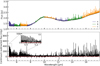 |
Fig. 1 JWST-MIRI MRS spectrum of DR Tau over channels 1 through 3 (4.9–17.98 µm). The different wavelength ranges (subbands) of each MIRI channel are indicated in the top panel in blue (‘A’), green (‘B’)> and orange (‘C’), respectively. The black line displays the estimated continuum. The bottom panel shows the continuum subtracted JWST-MIRI spectrum and contains a zoom-in on the CO transitions (4.9–5.3 µm). The red line in the bottom panel highlights the zero flux level. |
2.2 Continuum subtraction
Due to the line-richness of the DR Tau spectrum, we employed a different continuum subtraction method compared to Grant et al. (2023) and Gasman et al. (2023). The method here relies on a baseline estimation using the PYBASELINES package (Erb 2022). Before estimating the baseline, we masked downward spikes, such that they cannot influence the estimate. The downward spikes were masked using the following method: the continuum level was roughly estimated using a Savitzky–Golay filter, consisting of window sizes of 100 data points and polynomials of order 3. Through an iterative process, we removed all emission lines which extended above 2σ of the standard deviation (STD) of the Savitzky–Golay filter. Once no emission lines remained, we subtracted the final Savitzky–Golay filter and considered all 3σ downward outliers from the residuals as downward spikes. These downward spikes were subsequently masked from the baseline estimation on the full spectrum. The baseline was estimated using the ‘Iterative Reweighted Spline Quantiale Regression’ (IRSQR) method, which uses penalised splines and an iterative reweighted least squares technique to apply quantile (using a value of 0.05) regression. Within the method, we have used cubic splines with knots every 75 points and differential matrices of order 3.
The estimated baseline and continuum-subtracted spectrum are displayed in the top and bottom panel of Fig. 1, respectively. Appendix A shows and explains the intermediate steps from the applied continuum subtraction method.
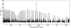 |
Fig. 2 Continuum-subtracted iSHELL spectrum of DR Tau. The wavelength gaps visible in the spectrum have either not been observed, or were removed due to interference from telluric lines. |
2.3 High-resolution CO observations
To complement the high- J levels of the CO P branch visible in the JWST spectrum at the shortest wavelengths (<5.3 µm), we have acquired high-resolution (R ≃ 60 000–92 000) IRTF-iSHELL (Rayner et al. 2016, 2022) data through SpExoDisks1 (Wheeler et al. in prep.). The iSHELL data were taken on January 23 2022 as part of a large M-band disk survey of planet-forming disks (Banzatti et al. 2022) and its water emission was analysed in Banzatti et al. (2023b). The data were flux calibrated using the allWISE catalogue (WISE-W2: λ = 4.6 µm, F = 1.91 ± 0.16 Jy; Wright et al. 2010; Cutri et al. 2013) and have been corrected for telluric features. As the allWISE flux calibration yields a small offset compared to the JWST-MIRI continuum, we have scaled the iSHELL observations by a factor ~0.71, assuming that the flux at ~5 µm is consistent across both observations. The required scaling may be the result of variability. However, as the iSHELL data were flux calibrated using WISE-W2 (λ = 4.6 µm), JWST-NIRSpec observations are required to properly investigate variability. As DR Tau is too bright to observe with JWST-NIRSpec, this comparison cannot be made. The data extend over the wavelength range from approximately ~4.516 µm to ~5.239 µm and cover ro-vibrational transitions of 12CO (υ = 1–0, υ = 2–1, and υ = 3–2) and 13CO (υ = 1–0), several H2O transitions, and the HI Pfund β (~4.655 µm) and Humphreys (~4.675 µm) lines. These data complement and extend upon the earlier VLT-CRIRES observations (at R ≃ 100 000), see Bast et al. (2011), Brown et al. (2013), and Banzatti & Pontoppidan (2015).
Similar to the continuum subtraction method described in Sect. 2.2, we subtracted the baseline using the IRSQR-method. However, for the iSHELL data we did not mask any downward spikes, we used a quantile regression with a value of 0.10, and we placed the knots every 100 data points. The continuum-subtracted iSHELL data are presented in Fig. 2. A comparison between the JWST-MIRI and iSHELL observations in the 4.9–5.1 µm region is displayed in Fig. 3.
3 Analysis
The following subsections provide an overview of the used techniques for obtaining the excitation properties. In Sect. 3.1, we describe our slab model retrieval process that has been used to characterise the emission from CO2, HCN, and C2H2 observed with JWST-MIRI. On the other hand, the techniques invoked for obtaining the CO line profiles and the rotational diagrams are described in Sect. 3.2.
3.1 LTE slab models
To extract information about the molecular features seen in the JWST-MIRI observations, we implement the same LTE slab model fitting procedure as described in Grant et al. (2023); Gasman et al. (2023); Perotti et al. (2023), and Tabone et al. (2023). We have obtained the required spectroscopic data through the HITRAN database (Gordon et al. 2022). Our slab models assume Gaussian line profiles with a broadening of ∆V = 4.7 km s−1 (σ = 2 km s−1), following Salyk et al. (2011b). In addition, we have accounted for the mutual shielding of adjacent lines in the Q branches of CO2, HCN, and C2H2 (see Tabone et al. 2023 for a description). We have convolved our CO2, HCN, and C2H2 models to a resolving power of ∆λ/λ ~ 2500. Finally, the SPECTRES package (Carnall 2017) was used to convolve the slab models to the JWST-MIRI wavelength grid.
The models consists of 3 free parameters that need to be varied to obtain the best fit to the molecular features: the column density N (in cm−2), the gas temperature T (in K) and the emitting area  , which is parameterised by the emitting radius Rem (in au). We note that while the slab models are parameterised by a circular area, the observed emission may have a different emission morphology with an equivalent area. For example, the emission can originate from an annulus with an area equal to
  .
.
To acquire the best combination of values for N, T, and Rem, we selected relatively isolated lines or regions of lines and used a reduced χ2 analysis to fit the slab models to these lines:
 (1)
(1)
Here, Nobs denotes the number of data points that were used for the fits, while Fobs and Fmod are, respectively, the observed and modelled continuum-subtracted fluxes, σ is the estimated noise. As opposed to Grant et al. (2023) and Gasman et al. (2023), we have not estimated the noise from line-free regions, as those are not present in the extremely line-rich spectrum of DR Tau. Instead we base our values for σ on the median continuum flux level in each combination of channels and ranges, and divide this by the highly idealised signal-to-noise ratio (S/N) acquired through the JWST Exposure Time Calculator (ETC)2. The median flux, obtained uncertainty and the estimate from the ETC for each subband can be found in Table B.1. To account for the regions covering multiple subbands, we use a weighted average of the estimated uncertainties for each respective band. The adopted weights represent the number of data points used from each subband in the χ2-analysis and this yields a different value for σ for each molecule. We list the range of σ values for the molecules detected in Table 1. Our derived values for σ are higher than those found for GW Lup (σ ~ 0.4 mJy in Channel 3; Grant et al. 2023) and Sz 98 (σ ~ 1.8–9.6 mJy; Gasman et al. 2023), due to our adopted method. The confidence intervals for our fits are defined as  and
and  for 1σ, 2σ, and 3σ, respectively (Avni 1976; Press et al. 1992).
Throughout our χ2 analysis we have used models based on the following grids for N, T and Rem: N ranged from 12 to 22 in log10-space, where we used a spacing of Δ (log10 (N) = 0.1. For T, we have used a spacing of ΔT = 25 K and a range of 150 ≤ T ≤ 2500 K. We note that Rem was allowed to vary between 0.01 au and 10 au, using steps of ΔR = 0.02 au.
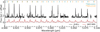 |
Fig. 3 Comparison between the JWST-MIRI (red) and iSHELL (black) data within the wavelength region of 4.9–5.1 µm, to highlight the differences in flux and resolution. The iSHELL observations are offset by 0.75 Jy. The vertical lines at the top of the plot indicate the positions of the 12CO υ = 2−1 (teal) and 13CO υ = 1−0 (orange) transitions, to highlight the main contributors of the secondary CO emission peaks visible in this wavelength region. |
Parameters of the best-fitting slab models for the different molecules observed with JWST-MIRI.
3.2 CO line profiles and rotational diagrams
To obtain information about T, N, and R from the high-resolution ro-vibrational transitions of 12CO and 13CO we carried out a rotational diagram analysis on the integrated fluxes, following the method described in Appendix A of Banzatti et al. (2012). We note that rotational diagram analyses and slab model fitting procedures are inherently the same, as long as the assumption of LTE is valid. We have assumed a Doppler broadening of δV = 1 km s−1. We note that using the same broadening as for the JWST-MIRI slab models (δV = 4.7 km s−1) in the rotational diagram analysis, the same excitation temperatures are inferred. However, the resulting column densities and emitting radii are found to be, respectively, higher and lower, while the total number of molecules is increased by less than 5%.
The required integrated fluxes have been obtained by, first, creating a weighted-averaged, normalised line profile, using the transitions that are unblended, not affected by telluric features, and have a high S/N. For the weighted average, we have used the errors on the flux as the weights. The line profile has been used to acquire one fixed value for the slight velocity offset (ΔV) from the heliocentric velocity (~27.6 km s−1; Ardila et al. 2002) and for the FWHM.
For the ro-vibrational ladders of 12CO (υ = 1−0, υ = 2−1, and υ = 3−2; see Sect. 4.2.2), we find that the line profile consists of two components: a narrow one, likely tracing an inner disk wind, and a broad one that traces the Keplerian rotation of the inner disk, as previously observed in Bast et al. (2011) and Brown et al. (2013). For these double components, we have used a double Gaussian line profile, whereas for the 13CO υ = 1−0 transitions we have used a single Gaussian line profile. The line profiles were fitted using the python-package LMFIT (Newville et al. 2014). These line profiles have been used to obtain the integrated fluxes of a larger set of transitions, including lines that are partly blended with other transitions and/or have a lower S/N. For 12CO υ = 3−2, no blended transitions are included, as we were unable to extract reasonable (compared with respect to the unblended lines) fluxes. The integrated fluxes have been acquired using the method described in Banzatti et al. (2012), based on the techniques provided in Pascucci et al. (2008); Najita et al. (2010) and Pontoppidan et al. (2010). In short, we invoke 1000 iterations of adding normally distributed noise to the observed flux. For each iteration, we determine the integrated flux and, subsequently, acquire a Gaussian distribution of measured line fluxes. We use the median of this distribution as the actual line flux and take the FWHM as the uncertainty.
To obtain information about both components, we carried out the rotational diagram analysis for all observed components separately. If the rotational diagrams consist of a straight line, the excitation temperature can be derived from the inverse of the slope of a fitted straight line, whereas the column density is given by the intercept. If the diagrams display curvature, which is an indication of optically thick emission (see Sect. 4.2.3), slab models must be used to properly derive the excitation conditions. Similarly as above, we have obtained the CO spectroscopic data from the HITRAN database. The best fitting values for T, N, and Rem have, similar to the slab-model fitting procedure, been acquired through a χ2-analysis, where σ in Eq. (1) now denotes the acquired error on the integrated flux. For the iSHELL data, we have used slightly different grids for the column density and temperature, but with the same step sizes: 14 ≤ log(N) ≤ 22 cm−2, 300 ≤ T ≤ 3000 K. For the emitting radius we adjusted both the grid and the stepsize into, respectively, 0.01 ≤ Rem ≤ 1 au and ∆Rem = 0.001 au. We have used the same grid for the different isotopologues and vibrational transitions.
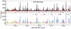 |
Fig. 4 Best-fitting slab models of 12CO2, HCN, and C2H2 in the 13.6–16.3 µm wavelength region. The top panel displays the continuum subtracted JWST spectrum in a specific region, while the full model spectrum is shown in red. In addition, the horizontal bars show for each molecule the spectral windows used in the χ2 fits. The bottom panel shows the models for the individually detected molecules. The H2O and OH slab models are shown for completeness. Their model properties will be presented in Temmink et al. (in prep.) |
4 Results
We present the results of our analysis in the following subsections. In particular, we highlight the observed molecular species with JWST-MIRI (CO2, HCN, and C2H2) in Sect. 4.1 and we provide an extensive analysis of the CO emission in Sect. 4.2, including our results regarding the excitation conditions, the line profiles, the optical depth, and the emitting radius.
4.1 JWST spectrum and detected molecules
The JWST-MIRI spectrum of DR Tau presented in Fig. 1 is very line-rich. Most of the visible lines correspond to H2O transitions, which will be analysed in Temmink et al. (in prep.). Here, we focus on the molecules, besides H2O and OH, for which transitions are covered by JWST-MIRI. The bottom panel of Fig. 1 also contains a zoom-in on the CO transitions (J ≥ 25), highlighting the strong emission features.
We detect emission from CO, CO2, HCN, and C2H2. Table 1 displays the parameters of the best fitting slab models for CO2, HCN, and C2H2. The uncertainties listed have been derived from the minimum and maximum value for each parameter that falls within the 1σ-confidence interval. We also list the total number of molecules (𝒩), which is well constrained for optically thin emission. The total number of molecules has been calculated by multiplying the column density with the emitting area:  . The best fitting slab models are displayed in Fig. 4, whereas the χ2-maps are shown in Fig. C.1.
4.1.1 12CO2
The Q branch of 12CO2 is well detected in DR Tau, whereas individual P- and R branch, and the hot-bands are not strongly detected. Our fit only extends over the Q branch, which yields a column density of N = 1017.4 cm−2, a gas temperature of T = 325 K and an emitting radius of R = 0.53 au. Compared to H2O, our 12CO2 Q branch is significantly weaker. This is similar to Sz 98 (Gasman et al. 2023) and EX Lup (Kóspál et al. 2023), but totally the opposite for GW Lup (Grant et al. 2023) and PDS 70 (Perotti et al. 2023). The difference with GW Lup is also visualised in Fig. 5, which displays a zoom-in on the normalised 12CO2 Q branch. As opposed to GW Lup, we do not detect any emission signature from 13CO2.
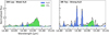 |
Fig. 5 Zoom-in on the 12CO2 Q branch (14.80–15.05 µm) of GW Lup (left; Grant et al. 2023) and DR Tau (right). Both spectra have been scaled to a common distance of 150 pc and normalised to the peak of the 12CO2 Q branch. |
4.1.2 HCN and C2H2
Similar to GW Lup (Grant et al. 2023), but contrarily to PDS 70 (Perotti et al. 2023), we detect HCN and C2H2 in the wavelength region of 13.6–16.3 µm. The HCN Q branch (~14 µm) and hot-band (~14.3 µm) are both strongly detected. The emission is likely optically thin, which causes the column densities and emitting radius to be degenerate (see also Fig. C.1). Nonetheless, our best-fitting slab model suggests a column density of N = 1014.7 cm−2, a temperature of T = 900 K, and an emitting radius of R = 4.83 au.
The parameters of C2H2 (~13.7 µm) are much less constrained compared to those of HCN. Similar to GW Lup, the inferred column density is on the border between optically thin and thick, which adds another degeneracy: for high column densities, there is a degeneracy between the column density and the gas temperature. For C2H2 we find a best-fitting column density of N = 10150 cm−2, a temperature of T = 775 K, and a emitting radius of R = 1.45 au.
4.2 CO analysis
As the main focus of this paper is the CO emission and a comparison between the JWST-MIRI and IRTF-iSHELL observations, this following section presents the results of the extensive CO analysis.
4.2.1 12CO as seen by JWST-MIRI
For molecules, such as CO, with well identified individual rovibrational lines, the excitation is commonly analysed by plotting the integrated fluxes in a rotational diagram. Figure 6 shows in green the measured JWST-MIRI fluxes of 12CO using a pseudo-Voigt profile (Labiano et al. 2021), assuming that the observable flux originates in the υ = 1−0 lines, that is, we ignore any blending with the 12CO υ = 2−1, υ = 3−2, and 13CO υ = 1−0 transitions. Recall that JWST-MIRI only probes the transitions with the largest J values (J ≥ 25) of the 12CO P branch.
The temperature, Tex, derived from such a rotational is given by the inverse of the slope, whereas the column density can be obtained from the intercept. For 12CO, we acquire a temperature as high as  K and a column density as low as 1.3 × 1017 cm−2 assuming an emitting area with a radius of 0.4 au (see Table 2). However, this simple analysis assumes that the line emission is optically thin. If the emission is optically thick, the inferred temperature can be much higher than the actual kinetic temperature. As demonstrated by, for example, Herczeg et al. (2011; see their Appendix D) and Francis et al. (2024), optically thick line emission introduces a curvature at medium J values. This curvature causes the high-J transitions (probed by JWST-MIRI) to mimic much higher excitation temperatures than the kinetic one when only those transitions are fitted in a diagram.
We emphasise this point by including the integrated iSHELL fluxes of the 12CO υ = 1−0 transitions in Fig. 6, with the black and red squares obtained by taking the sum over the narrow and broad components. The red squares mark the transitions that are observable with JWST-MIRI and, as seen in the figure, some small differences are visible in the measured fluxes with respect to JWST-MIRI, as we have not accounted for the blending of lines in the JWST-MIRI spectrum. As shown in Fig. D.5, many of the 12CO υ = 1−0 transitions are blended with other lines, while only a handful are unblended, some of which are highlighted in Fig. D.5, whereas a few more can be found at longer wavelengths (≥5.18 µm). Such blending will be worse for sources with higher intrinsic line wings (e.g. sources with outflows or galaxies), where one may not be able to detect any unblended line at all.
The iSHELL fluxes clearly show a curvature in the rotational diagrams. For comparison, we fitted a straight line to the iSHELL integrated fluxes that cover the JWST-MIRI wavelength range (the red squares). The fit yields an excitation temperature of Tex = 2992 ± 40 K. As will be demonstrated in Sect. 4.2.2 (see Table 2), the inferred temperatures are much lower when the iSHELL observations are fitted over the full range of J values with a LTE slab model that accounts for optical depth. This demonstrates the importance of having information on the fluxes of the lower-J lines.
As mentioned before, JWST-MIRI’s resolution is not sufficient to distinguish between the two components present in the complex line profile of 12CO. The total 12CO line profile can, on the other hand, only be marginally resolved with JWST-MIRI. For unblended 12CO v = 1 − 0 transitions (see Sect. 4.2.6), we infer values for the FWHM in the range of ~84–100 km s−1, which are slightly larger than JWST-MIRI’s velocity resolution of ~80 km s−1 (Labiano et al. 2021). The narrow component, tracing the disk wind, could potentially be observed with JWST-MIRI as extended emission. However, no extended emission is observed in the CO lines.
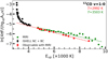 |
Fig. 6 Rotational diagram of the 12CO υ = 1−0 transitions. As JWST-MIRI is unable to distinguish between the narrow (NC) and broad (BC) components, their contributions have been added together. The black squares indicate the fluxes inferred from the iSHELL observations, while the ones marked denote the transitions that are also observable with JWST-MIRI. Errorbars on the iSHELL observations are plotted, however, these are too small with respect to the size of the squares. The circles in green are the integrated fluxes inferred from the JWST-MIRI observations using a pseudo-Voigt profile. The red, dashed line is a fit to the red points, used to derive what excitation temperature JWST-MIRI would probe as seen with the iSHELL observations (T = 2992 ± 40 K). The green dashed line indicates the excitation temperature derived from these observations, |

Best fit parameters acquired through the rotational diagram analysis for the iSHELL data.
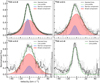 |
Fig. 7 Fitted iSHELL line profiles for the CO υ = 1−0, υ = 2−1, υ = 3−2, and the CO υ = 1−0 transitions. The median line profile is shown in black, whereas the fitted line profile is shown in green. For the 12CO transitions, we have indicated the narrow and broad components in, respectively, blue and red. The faint, grey line profiles visible in the background correspond to the individual line profiles used in creating the weighted−averaged, normalised line profile. |
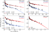 |
Fig. 8 Rotational diagrams for 12CO υ = 1−0 (top left), υ = 2−1 (top right), υ = 3−2 (bottom left), and 13CO υ = 1−0 (bottom right). In each panel, the slab models are given by the solid line. For the 12CO transitions, the narrow and broad components (NC and BC, respectively) are shown separately. The integrated fluxes for the narrow component are given by the dots, while those for the broad component are indicated by the squares. The two lines in each model correspond the R- and P branches. |
4.2.2 iSHELL CO line profiles and rotational diagrams
A proper analysis of the high-resolution, ground-based CO observations starts with a thorough analysis of the line profiles. The line profiles are displayed in Fig. 7, whereas the acquired values for ∆V and the FWHM are listed in Table 2. The rotational diagrams themselves are displayed in Fig. 8, while the best-fit parameters, for the broad and narrow components, are summarised, together with the values for the average FWHM and ∆V, in Table 2. The rotational diagrams (Fig. 8) of the 12CO vibrational ladders and 13CO v = 1 − 0 transitions are presented separately. In addition, we separated out the narrow and broad components for 12CO. For the broad component we find consistently higher integrated fluxes and excitation temperatures compared to those of the narrow one. All diagrams display an upward curvature at the lower end of the Eup range, suggesting optically thick emission. Optical depth is further discussed in Sect. 4.2.3. We do not list any uncertainties on the best fitting parameters (T and N), but they can be viewed in Fig. D.2. Models, based on the rotational diagrams, for the transitions of 12CO v = 1−0 (red), v = 2−1 (blue), v = 3−2 (green), and 13CO v = 1−0 (yellow) are displayed in Fig. D.1, while a zoom-in on the 4.68–4.72 µm region is shown in Fig. 9, to provide a better view of how well the model fits the data.
We find column densities in the range of 1.6 × 10¹⁷−5.0 × 1018 cm−2 for the different transitions and temperatures of 725–2175 K. We find that the narrow components of the various 12CO ro-vibrational transitions trace colder temperatures (respectively, 1000, 1050, and 1800 K) compared to the broad components (respectively, 1725, 2175, and 2025 K), confirming the different origins of the two components and suggesting that the broad component does trace the hot inner regions of the disk. For 13CO we find a significantly lower temperature of 725 K, which is slightly higher than the value reported by Bast et al. (2011) and Brown et al. (2013) of T = 510–570 K. However, both Bast et al. (2011) and Brown et al. (2013) used only transitions with Eup ~ 3000–4000 K, whereas our data include transitions with values of Eup up to ~6200 K.
4.2.3 Optical depth: 12CO and 13CO
As previously found by Brown et al. (2013), the 12CO emission of DR Tau is optically thick. Similarly as their Fig. 11, Fig. D.3 displays the rotational diagrams of the 12CO υ = 1−0, where we have combined the narrow and broad components, and 13CO υ =1−0 transitions together. In addition, we have multiplied the best fitting model of 13CO by a factor of 68 to account for the isotopologue ratio as in the solar neighbourhood (Milam et al. 2005; 12C/13C = 68 ± 15). If 12CO were opticaüy thin, the scaled 13CO model would have coincided with the 12CO fluxes. However, we see that the scaled 13CO lies above the 12CO fluxes, confirming in a similar manner as Brown et al. (2013) that 12CO is optically thick. Furthermore, 12CO being optically thick is also confirmed by the shape of the line fluxes. As shown by Herczeg et al. (2011; see their Fig. D.1), for optically thin emission one would expect a straight line, whereas if the emission becomes optically thick the fluxes of the lines with higher upper level energies flatten off. Furthermore, as seen in Fig. D.3, the 13CO υ =1−0 model is also not completely a straight line, suggesting that the 13CO is also (moderately) optically thick. However, as the 13CO emission is less optically thick, a better lower limit on the total number of molecules can be obtained by multiplying the total number of molecules found for 13CO by the isotopologue ratio of 68. This multiplication yields a total number of molecules of 𝒩CO ≃ 1.6 × 1045.
As the 13CO emission is also (moderately) optically thick, rarer, less optically thick isotopologues are needed to infer the total amount of molecules. While C18O is not detected in the iSHELL observations, the υ = 1−0 transitions are detected in the VLT-CRIRES data of Bast et al. (2011). For a description of the data, we refer to Bast et al. (2011) and Brown et al. (2013). We also scale the VLT-CRIRES data to match the JWST-MIRI flux at ~5 µm. Using the same approach as described in Sect. 2.3, we carry out a rotational diagram analysis for the C18O υ = 1−0 transitions to obtain a better estimate for the total number of molecules.
First, for the C18O line profile we find a velocity offset of ∆V = −4.2 km s−1 with respect to DR Tau’s heliocentric velocity and a FWHM of 10.3 km s−1. Second, the rotational diagram yields an excitation temperature of T = 975 K, a column density of N = 2.0 × 1016 cm−2, and an emitting radius of Rem = 0.23 au. The acquired line profile and rotational diagram are displayed in, respectively, the left and right panel of Fig. 10. The χ2-map, visualising the uncertainties of the fit, is shown in the bottom right panel of Fig. D.2. The inferred excitation temperature for C18O is found to be higher than that of 13CO. However, the χ2-maps of C18O show a large contour for the 1σ uncertainty, suggesting that the temperatures agree within the uncertainties. Finally, multiplying the column density by the corresponding emitting area yields a total number of molecules of 𝒩 = 7.4 × 1041, which multiplied by the isotopologue ratio of 16O/18O = 557 ± 30 (Wilson 1999) yields 𝒩CO = 4.1 × 1044.
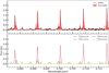 |
Fig. 9 Zoom-in (4.68–4.72 µm) of the continuum-subtracted iSHELL spectrum of DR Tau with a model based on the best-fitting parameters obtained through the rotational diagram analysis. A full version can be found in Fig. D.1. |
4.2.4 Estimated emitting radii of CO
Previous studies (e.g. Salyk et al. 2011a; Banzatti & Pontoppidan 2015; Banzatti et al. 2022) have shown that the emitting radius where the line flux peaks can be estimated from the line profiles using Kepler’s law, as the emission is broadened by the Keplerian rotation:
 (2)
(2)
where i is the inclination and ∆v is the line width, often taken to be equal to the half width at half maximum (HWHM). The inner emitting radius can, subsequently, also be estimated by taking ∆υ equal to the half width at 10% (HW10%; Banzatti et al. 2022). Both the HWHM and the HW10% have been derived from the averaged line profiles displayed in Fig. 7, for simplicity we have taken the HWHM equal to half the FWHM listed in Table 2. Assuming the inclination of the inner disk of DR Tau to be equal to the inclination of the outer disk, we use i = 5.4º (Long et al. 2019). Furthermore, as this method only applies to the lines broadened by the Keplerian rotation, we calculate the (inner) emitting radius only for the broad components of the different 12CO line profiles and the 13CO υ = 1−0 line profile. The calculated values are listed in Table 3.
All the calculated emitting radii (RCO) differ significantly from those inferred through the rotational diagrams. One potential explanation for the differences can be found in the chosen value for the inclination. The used inclination has been derived from the continuum emission as probed by ALMA. However, inner disks can be misaligned with respect to the outer disk, for instance caused by perturbations induced by companions (see, for example, Bohn et al. 2022). By testing a wide variety of larger inclinations, we infer that inclinations of, respectively, 20.1º, 22.4°, 23.0°, and, 10.2° are required to match the corresponding emitting radii for the broad components of the various 12CO vibrational transitions and the 13CO υ =1−0 transitions inferred from the rotational diagrams. This holds for the assumption that these emitting radii correspond to circular area enclosing the host star. As the high inferred excitation temperatures suggest that the emission of the broad component must originate from inside the dust sublimation radius, this assumption may be valid for DR Tau. Such a higher inferred inclination of the inner disk agrees with the value of  derived by GRAVITY Collaboration (2021) using VLTI-GRAVITY observations. It must be noted, however, that the uncertainties on this inclination also encompass the inclination of the outer disk
  . Although this cannot yet be confirmed, the VLTI-GRAVĪTY observations and the CO line profiles both hint at a misalignment between the inner and outer disk.
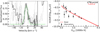 |
Fig. 10 Inferred Gaussian line profile (left panel) and rotational diagram (right panel) for the C18O υ = 1−0 transitions. The rotational diagram yields an excitation temperature of T = 975 K. |
Derived (inner) emitting radii for the ro-vibrational transitions of 12CO and 13CO using an inclination of i = 5.4°.
4.2.5 LTE versus non-LTE
When using slab models or creating rotational diagrams, LTE is (almost) always assumed, but the question remains whether this is a valid assumption. A simple test to see if all 12CO emission lines can be characterised by a single temperature can be carried out by using the 12CO v =1−0 best-fit parameters for the v =2−1 transitions. If the υ =1−0 parameters reproduce the observed υ =2−1 fluxes, the emission can be considered in LTE. Otherwise, the vibrational excitation is in non-LTE and the various transitions need to be considered separately, as we have done for the high-resolution observations. The right panel of Fig. D.4 shows the model prediction of the 12CO υ =2−1 transitions using the best-fit parameters of the υ =1−0 transitions (see Table 2). As can be seen, the model overpredicts the emission of the 12CO υ =2−1 transitions, confirming that the vibrational excitation is not in LTE. The various vibrational transitions thus need to be considered separately, while the rotational populations can still be in LTE.
Our findings are not surprising, considering the work by Bast et al. (2011). They find a higher vibrational temperature (T ~ 1700 K) for DR Tau, while only a temperature of T ~ 500 K for the rotational 13CO lines. Higher vibrational temperatures are more commonly found for Herbig Ae/Be stars (e.g. Brittain et al. 2007 and van der Plas et al. 2015), which may be attributed to their higher UV fields and subsequent UV-pumping into the higher vibrational states. For T-Tauri stars, UV-pumping into the higher vibrational states can be achieved through higher UV fluxes following accretion by the host star (Valenti et al. 2000). As DR Tau is known to be an actively accreting system, UV-pumping provides a possible explanation for the higher vibrational temperatures found by Bast et al. (2011).
4.2.6 Implication for JWST-MIRI analysis
While the LTE slab model of 12CO fitted to the JWST-MIRI observations (see Table 1) roughly agrees with the excitation parameters found for the 12CO υ =1−0 broad component (see Table 2), these results must be treated with caution. As mentioned before, the JWST-MIRI observations do not have the spectral resolution to distinguish between the broad and narrow components observed for 12CO and, as discussed in Sect. 4.2.5, the CO emission is not in LTE, suggesting that the observed emission cannot be described by a single temperature. In the following section, we explore how the slab models fitted to the rotational diagrams of the iSHELL observations can be used to describe the CO emission as observed by JWST-MIRI.
The main difference between the JWST-MIRI and iSHELL observations is the spectral resolution of JWST-MIRI, which does not allow one to distinguish between the narrow and broad components (this also holds for JWST-NIRSpec), as displayed in Fig. 7. In addition, as mentioned before, the JWST-MIRI observations only cover the high-J transitions of the P branch. The excitation temperature as probed by JWST-MIRI would, subsequently, not only be affected by the combination of both components (likely approaching the weighted average of the two), but would also be biased to higher excitation temperatures following the inclusion of only transitions with high upper level energies. As discussed in Sect. 4.2.1 and displayed in Fig. 6, a temperature of ~2992 K is acquired from the lines covered by JWST-MIRI, which is significantly higher than probed by the high-resolution iSHELL observations. Additionally, as shown in Fig. 3, various transitions that are unblended in the iSHELL spectrum are blended in the JWST-MIRI one. Subsequently, it is harder to identify the contributions from the various (vibrational) transitions in JWST-MIRI’s spectrum.
To be able to compare the CO emission observed with iSHELL and JWST-MIRI, and, more importantly, to show that we probe the same emission with both instruments, we bin our iSHELL model to JWST-MIRI’s lower spectral resolution and convolve the binned model with JWST-MIRI’s line profile. The binning was carried out using the python-package SPECTRES, whereas the convolution was implemented using ASTROPY and a kernel based on JWST-MIRI’s line profile. As discussed in Labiano et al. (2021), JWST-MIRI’s line profile is best described by a pseudo-Voigt profile, which is a weighted sum between a Gaussian and a Lorentzian profile (see Eq. (3)). In comparison, a normal Voigt profile is given by the convolution of a Gaussian and Lorentzian profile. To create the convolution kernel, we first identified the strongest, unblended 12CO υ = 1−0 transitions in the JWST-MIRI spectrum. These lines are displayed in Fig. D.5. Subsequently, we created an average, normalised line emission profile, which is displayed in Fig. D.6, by considering the 7 resolution elements enclosing the line peaks (blue shaded areas in Fig. D.5). Finally, we used LMFIT to fit a pseudo-Voigt profile to the averaged emission, which is also shown in Fig. D.6. The fitted pseudo-Voigt profile was, subsequently, adopted as our convolution kernel.
The used pseudo-Voigt profile is described by the following equation:
![Mathematical equation: $f\left( {x;A,\mu ,{\sigma _f},\alpha } \right) = {{(1 - \alpha )A} \over {{\sigma _{\rm{g}}}\sqrt {2\pi } }}{e^{ - {{(x - \mu )}^2}/2\sigma _{\rm{g}}^2}} + {{\alpha A} \over \pi }\left[ {{{{\sigma _f}} \over {{{(x - \mu )}^2} + \sigma _f^2}}} \right].$](/articles/aa/full_html/2024/06/aa48911-23/aa48911-23-eq21.png) (3)
(3)
Here, A denotes the amplitude, µ the center of the line, σf describes the width, and α gives the weights. Furthermore, σg is defined as  . Table 4 gives the best fitting values and their confidence intervals for A, µ, σf, and α.
Figure 11 shows our results: the top panel shows the full CO model on top of the iSHELL observations, whereas the middle and bottom panel shows the model on top of the JWST-MIRI data after applying the binning and convolution, respectively. As clearly shown in the middle panel, solely binning the high-resolution model down to JWST-MIRI’s resolution does not provide a good fit, as the peak flux is clearly overproduced. The subsequent convolution, on the other hand, yields a good description of the JWST-MIRI observations, as is shown in the bottom panel. To conclude, by binning a high-resolution model to JWST-MIRI’s spectral resolution and by convolving the model with JWST-MIRI’s line profile, we have shown that the high-resolution observations can be used as a good template for the JWST-MIRI observations and that a proper treatment of the line profile is crucial.
We note that, even after convolution, the model does not provide a perfect fit to the JWST-MIRI observations. The small residual differences are potentially related to uncertainties of the flux calibration of the iSHELL observations or the different sensitivities of the instruments. In addition, stellar variability at the 20% level cannot be excluded as an explanation. Nonetheless, we have shown and argue that the best way to characterise the CO lines observed with JWST-MIRI is to combine them with high spectral resolution observations of ground-based instruments, such as iSHELL or VLT-CRIRES(+), that are publicly available for many sources through SpExoDisks.
Best-fitting values and the corresponding confidence intervals for the pseudo-Voigt profile used to characterise the JWST-MIRI line profile.
4.2.7 JWST-MIRI line profile: Pseudo-Voigt versus Gaussian
As line profiles are often considered to be of pure Gaussian nature, we discuss in the this subsection the different results one may acquire when treating JWST-MIRI’s line profile as a Gaussian. When using a Gaussian line profile, we derive integrated fluxes that are 10% or less smaller than those acquired when using a pseudo-Voigt profile. Figure D.7 compares the JWST-MIRI rotational diagrams when considering the different line profiles. A straight line fitted to the Gaussian integrated fluxes yields an excitation temperature of  , which is slightly higher than the one
  probed when using a pseudo-Voigt profile. The temperatures do, however, agree well within the uncertainties.
In addition, we reproduce the analysis conducted in Sect. 4.2.6 for a Gaussian line profile, given by the first part of Eq. (3) (setting α = 0). Figure D.6 contains the fitted Gaussian line profile to the normalised, unblended 12CO transitions, which is described by the following parameters: A = 2.40, µ = 2.85, and σ𝑔 = 0.98. The bottom panel of Fig. D.8 shows the convolution of the binned CO model with the Gaussian line profile. A close visual comparison between Figs. 11 and D.8 yields only small differences between the two convolutions: the main difference can, as expected, be found in the line wings of the convolved model. The Lorentzian contribution ensures that the pseudo-Voigt profile provides a better fit to the line wings compared to the Gaussian one. On the other hand, the Gaussian convolution can yield a model with slightly higher peak values, as less flux is distributed over the line wings.
Even though the Gaussian convolution yields similar results as the pseudo-Voigt one, the pseudo-Voigt profile, as found by Labiano et al. (2021), provides a significantly better description of the JWST-MIRI observations in subband 1A, as demonstrated by Fig. 11. Depending on the application, a Gaussian profile may provide a sufficient fit to the observations, but one must take into consideration that the flux in the line wings will be underproduced.
An incorrect treatment of the line profile can also impact the analysis of the excitation conditions, as the underproduced line wings may result in an underestimation of the line fluxes. For example, the integral of the Gaussian line profile displayed in Fig. D.6 is ~5% lower than that of the Pseudo-Voigt line profile. Consequently, a rotational diagrams analysis can yield a lower value on the total column density and a different value for the excitation temperature, depending on how the slope is changed by these underestimated fluxes.
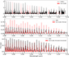 |
Fig. 11 Top panel: continuum-subtracted iSHELL data (black) with the best-fitting model (red) based on the various slab model fits to the rotational diagrams over the 4.90–5.25 µm wavelength region. The middle panel shows the best fitting model binned to the JWST-MIRI resolution together with the JWST-MIRI observations, whereas the bottom panel shows the model convolved with the pseudo-Voigt profile shown in Fig. D.6. |
5 Discussion
5.1 CO excitation temperature as probed by JWST-MIRI
As shown in Fig. 6, the excitation temperature derived when only considering the high-J transitions observed by JWST-MIRI, assuming optically thin emission, is significantly higher than that derived from a rotational diagram that includes also lower-J values. As discussed in Sect. 4.2.1, the higher excitation temperature follows from the fact that the 12CO emission is optically thick. We emphasise the need for complementary observations when deriving the excitation properties of CO, either from space (e.g. with JWST-NIRSpec) or from the ground (e.g. with VLT-CRIRES(+), IRTF-iSHELL or Keck-NIRSPEC). If only space-based observations are used, we advise to treat the results with caution, since JWST-NIRSpec and JWST-MIRI do not have the spectral resolution to resolve the commonly observed, complex CO line profiles of planet-forming disks (see also Banzatti et al. 2022, 2023b).
5.2 Emitting region of CO
The high inferred excitation temperatures of T ≥ 1725 K suggest that the broad component of the 12CO emission must come from inside the dust sublimation radius (Tdust ≃ 1500 K) as also indicated in Fig. 14 of Banzatti et al. 2022). Alternatively, the emission may originate from an elevated layer of the disk’s atmosphere, where the gas temperature can be well above that of the dust. The 13CO emission, on the other hand, should trace a deeper layer of the disk, as it is less optically thick compared to 12CO, consistent with the lower probed excitation temperature. Depending on the flaring of the inner disks, the emission originating from these elevated emitting layers (as seen from the disk’s midplane) could also explain the larger inclinations, or viewing angles, required for the emitting radii derived from the CO line profiles and slab models fitted to the rotational diagrams to match. Alternatively, a misalignment between the inner and outer disks, as hinted at by the VLTI-GRAVITY and ALMA observations, may also explain the required inclinations.
Thermo-chemical models have shown that the gas temperature in the inner regions of T-Tauri disks, in particular the elevated layers, can reach temperatures of ≥1000 K (Thi et al. 2013; Bruderer et al. 2015; Walsh et al. 2015; Woitke et al. 2018). These high temperatures further strengthen the notion that the CO emission must originate from the region inside of the dust sublimation radius and/or elevated layers of the disk.
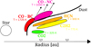 |
Fig. 12 Cartoon visualising the expected emission regions, based on the slab models and interpreting the emitting radius as the disk radius, for our investigated molecules (CO, CO2, HCN, and C2H2). |
5.3 Comparing the emitting properties of CO with the other molecules
Compared with the other molecules studied here, CO2, HCN, and C2H2, the excitation temperatures probed by CO are much higher. It must be noted that the temperatures inferred for CO2, HCN, and C2H2 are similar to those in the other T-Tauri disks, GW Lup and Sz 98 (Grant et al. 2023; Gasman et al. 2023). Models by Woitke et al. (2018) suggest that the emission likely originates from an onion-like structure, where CO has the highest emitting height and C2H2 the lowest. CO2 and HCN originate from layers in between, with CO2 originating from a slightly higher layer than HCN. Based on the derived excitation temperatures, this is in partial disagreement with our slab modelling efforts, which suggest that the CO2 emission should originate from either a deeper emitting layer or from a larger radial distance compared to that of HCN and C2H2. The expected emission regions, based on our slab models, for the investigated molecules are visualised in Fig. 12. Since the same findings hold for the disks around GW Lup and Sz 98, additional (thermo)chemical modelling work is necessary to explain the observations and to infer from which layers these molecules originate from.
6 Conclusions and summary
In this work we have investigated the JWST-MIRI observations of the disk around the young star DR Tau. In addition, we have used complementary, high resolution CO ro-vibrational observations to fully investigate the emission properties of CO. Below we summarise our main conclusions:
We have confirmed the detections of CO, 12CO2, HCN, and C2H2 with JWST-MIRI, all of which have been observed before with Spitɀer and from the ground. With JWST-MIRI we are now able to better constrain the excitation conditions and find excitation conditions of 12CO2, HCN, and C2H2 for DR Tau that are similar to those derived for GW Lup and Sz 98. The conditions suggest that HCN and C2H2 originate from a layer higher up in the disk’s atmosphere than 12CO2.
Using high-resolution IRTF-iSHELL observations we have thoroughly analysed the CO emission properties using slab model fits to rotational diagrams. These observations cover various transitions of 12CO υ = 1−0, υ = 2−1, and υ = 3−2, and 13CO υ = 1−0. Similar to previous studies, we note that the 12CO transitions are comprised of two components: a narrow and a broad component. The narrow part is linked to a potential inner disk wind, whereas the broad component is thought to arise from the Keplerian rotation of the disk. The high inferred temperatures (≥1725 K) for the broad component of the 12CO transitions suggest that the emission likely originates from a high atmospheric layer and/or from inside the dust sublimation radius.
In addition to the emitting radii inferred from the slab models, we have calculated the emitting radii based on the line profiles, which are found to be significantly smaller than those inferred from the rotational diagrams. To match the emitting radii, we require higher inclinations (or viewing angles if the emission comes from a flared elevated layer) of the inner disk of i ~ 10-23°, suggesting, under the assumption that the inferred emitting radii correspond to a circular emitting area enclosing the host star, that the inner disk of DR Tau may be slightly misaligned with the respect to the outer disk (iouter ~ 5°).
Based on the flux ratios and curvature visible in the rotational diagrams, we find that the 12CO and 13CO transitions are optically thick. Using C18O transitions covered in VLT-CRIRES observations and applying the same rotational diagram analysis, we have inferred a total number of molecules for CO in the inner disk (≤0.23 au) of DR Tau: 𝒩CO ~ 4.1 × 1044.
Finally, we show that, to properly compare the JWST-MIRI and high-resolution, ground-based CO observations, one needs to bin the high-resolution model to JWST-MIRI’s spectral resolution and convolve the binned spectrum with a pseudo-Voigt profile.
With this work we emphasise that, although JWST-MIRI is a powerful instrument and is able to confidently detect the high-J transitions of CO, complementary, high-resolution observations are necessary to properly investigate the physical properties of the emitting gas. For DR Tau, the Keplerian CO emission must originate from inside the dust sublimation radius at temperatures of T ≥ 1725 K, close to the host star. Other molecules, such as 12CO2, HCN, and C2H2 are found to originate from farther out in the disk, with 12CO2 likely originating from the deepest layer in the disk of DR Tau. In addition, the slow disk wind, as traced by the narrow component of 12CO (T ≥ 1000 K), is launched from a larger radial distance compared to the Keplerian emission.
Acknowledgements
The authors would like to thank Andrea Banzatti for the many very useful discussions. This work is based on observations made with the NASA/ESA/CSA James Webb Space Telescope. The data were obtained from the Mikulski Archive for Space Telescopes at the Space Telescope Science Institute, which is operated by the Association of Universities for Research in Astronomy, Inc., under NASA contract NAS 5-03127 for JWST. These observations are associated with program #1282. The following National and International Funding Agencies funded and supported the MIRI development: NASA; ESA; Belgian Science Policy Office (BELSPO); Centre National d'Etudes Spatiales (CNES); Danish National Space Centre; Deutsches Zentrum fur Luft- und Raum-fahrt (DLR); Enterprise Ireland; Ministerio De Economía y Competividad; Netherlands Research School for Astronomy (NOVA); Netherlands Organisation for Scientific Research (NWO); Science and Technology Facilities Council; Swiss Space Office; Swedish National Space Agency; and UK Space Agency. This research used the SpExoDisks Database at www.spexodisks.com. M.T. and E.v.D. acknowledge support from the ERC grant 101019751 MOLDISK. E.v.D. acknowledges support from the Danish National Research Foundation through the Center of Excellence “InterCat” (DNRF150). B.T. is a Laureate of the Paris Region fellowship program, which is supported by the Ile-de-France Region and has received funding under the Horizon 2020 innovation framework program and Marie Sklodowska-Curie grant agreement no. 945298. D.G., V.C., I.A., A.O., and B.V. thank the Belgian Federal Science Policy Office (BELSPO) for the provision of financial support in the framework of the PRODEX Programme of the European Space Agency (ESA). V.C. and A.O. acknowledge funding from the Belgian F.R.S.-FNRS. G.P. gratefully acknowledges support from the Max Planck Society. T.H. and K.S. acknowledge support from the European Research Council under the Horizon 2020 Framework Program via the ERC Advanced Grant Origins 83 24 28. D.B. and M.M.C. have been funded by Spanish MCIN/AEI/10.13039/501100011033 grants PID2019-107061GB-C61 and No. MDM-2017-0737. A.C.G. acknowledges from PRIN-MUR 2022 20228JPA3A “The path to star and planet formation in the JWST era (PATH)” and by INAF-GoG 2022 “NIR-dark Accretion Outbursts in Massive Young stellar objects (NAOMY)” and Large Grant INAF 2022 “YSOs Outflows, Disks and Accretion: towards a global framework for the evolution of planet forming systems (YODA)”. I.K., A.M.A., and E.v.D. acknowledge support from grant TOP-1 614.001.751 from the Dutch Research Council (NWO). I.K. and J.K. acknowledge funding from H2020-MSCA-ITN-2019, grant no. 860470 (CHAMELEON). T.P.R. acknowledges support from ERC grant 743029 EASY. L.C. acknowledges support by grant PIB2021-127718NB-I00, from the Spanish Ministry of Science and Innovation/State Agency of Research MCIN/AEI/10.13039/501100011033.
Appendix A Continuum subtraction
This section provides the immediate steps of the continuum subtraction described in Section 2.2. The necessary images are shown in Figure A.1. The top panel of this figure shows the final Savitzky–Golay filter (green) after all >2σ emission lines (light grey) have been filtered, together with the line-filtered spectrum. The middle panel displays the residuals after subtracting the Savitzky–Golay filter from the line-filtered spectrum. The green lines indicate the -3× level of the STD of the residuals. All the red crosses indicate the data points that lie below the -3×STD lines and have, subsequently, been masked throughout the baseline estimation. Finally, the bottom panel shows the full JWST-MIRI spectrum, together with the estimated baseline, and the masked data points.
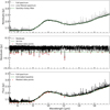 |
Fig. A.1 Intermediate steps of the continuum subtraction method described in Section 2.2. The top panel shows the final Savitzky–Golay filter (green) on the filtered line spectrum (black) and the filtered lines (light grey). The middle panel displays the residuals (black; line-filtered spectrum after subtracting the Savitzky–Golay filter), together with their -3×STD level (green), and the data points that fall below the -3× level (red crosses). The bottom panel shows the full JWST-MIRI spectrum (black) together with the estimated baseline (green) and the data points that have been masked throughout the estimation of the baseline (red crosses). |
Appendix B Uncertainties for the JWST-MIRI subbands
Median continuum flux, estimated S/N from the ETC, and the acquired uncertainty σ for each subband.
Appendix C χ2-maps of CO2, HCN, and C2H2
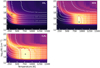 |
Fig. C.1 Normalised χ2 maps |

Appendix D Complementary CO ro-vibrational observations
D.1 Line information and integrated fluxes
Information on the CO transitions used for the rotational diagrams and corresponding integrated fluxes.
D.2 Full iSHELL model
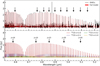 |
Fig. D.1 Continuum-subtracted iSHELL spectrum of DR Tau with a model based on the best-fitting parameters obtained through the rotational diagram analysis. The gaps visible (highlighted by the black arrows in the top panel) in the iSHELL spectrum correspond to removed telluric features. The top panel shows the full model, whereas the bottom panel shows the contribution of each band separately. For 12CO, the narrow and broad component are shown together. In addition, in the bottom panel we highlight the 12CO transitions which have an upper level J-value of 10, 20, 30, or 40. |
D.3 χ2-maps of the CO rotational diagrams
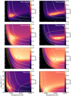 |
Fig. D.2 Similar as Figure C.1, but for the iSHELL CO rotational diagrams. The top row shows those for the narrow (left) and broad (right) component of 12CO v=1-0 transitions. Those for the 12CO v=2-1 and v=3-2 transitions are shown on the second and third row, respectively, whereas the ones for the 13CO and C18O (using VLT-CRIRES data) are shown on the bottom row. |
D.4 Optical depth of 12CO
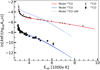 |
Fig. D.3 Rotational diagrams for 12CO v=1-0 (dots) and 13CO v=1-0 (squares). The dashed blue line indicates the model of 13CO (T = 750 K) multiplied by a factor of 68 to account for the isotopologue ratio. The fluxes shown for the 12CO are a summation of the narrow (T = 1000 K) and broad (T = 1725 K) components. |
D.5 LTE versus non-LTE
 |
Fig. D.4 Comparison between the rotational diagrams of the 12CO v=1-0 and v=2-1 transitions to test the assumption of LTE. The left panel shows the 12CO v=1-0 rotational diagrams (see also Figure 8). The right panel shows the non-LTE test, where the 12CO v=2-1 integrated fluxes are shown together with expected the models based on the results of the 12CO v=1-0 rotational diagrams. As the models overproduce the observed 12CO v=2-1 fluxes, invalidating the assumption that the levels can be characterised by a single temperature. |
D.6 Convolution iSHELL to JWST-MIRI resolution
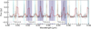 |
Fig. D.5 Xoom-in of Figure 3 on the JWST-MIRI data (red) within the wavelength region 4.90-4.98 µm. The iSHELL observations are shown here in grey. The different transitions in this wavelength region of the 12CO v=1-0 (dark blue), v=2-1 (teal), v=3-2 (cyan), and the 13CO v=1-0 (orange) transitions are shown to identify the different lines and highlight corresponding line overlaps. The dark blue shaded areas indicate the (relatively) isolated 12CO v=1-0 transitions that have been used to determine the pseudo-Voigt line profile of the JWST-MIRI data. |
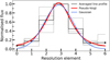 |
Fig. D.6 Averaged, normalised line profile of the four selected, unblended 12CO v=1-0 transitions observed with JWST-MIRI (see also Figure D.5. The faint grey lines indicate the individual, normalised lines, whereas the red and blue lines display, respectively, the fitted pseudo-Voigt and Gaussian profiles. |
D.6.1 Gaussian line profile
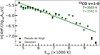 |
Fig. D.7 Simple rotational diagrams of the JWST-MIRI integrated fluxes when considering a pseudo-Voigt (black) or a Gaussian (green) line profile. Straight line fits suggest excitation temperatures of T = 3503 K when considering the pseudo-Voigt profile and T = 3565 when using a Gaussian. |
References
- Andrews, S. M., Huang, J., Pérez, L. M., et al. 2018, ApJ, 869, L41 [NASA ADS] [CrossRef] [Google Scholar]
- Ardila, D. R., Basri, G., Walter, F. M., Valenti, J. A., & Johns-Krull, C. M. 2002, ApJ, 567, 1013 [NASA ADS] [CrossRef] [Google Scholar]
- Argyriou, I., Glasse, A., Law, D. R., et al. 2023, A&A, 675, A111 [NASA ADS] [CrossRef] [EDP Sciences] [Google Scholar]
- Avni, Y. 1976, ApJ, 210, 642 [NASA ADS] [CrossRef] [Google Scholar]
- Banzatti, A., & Pontoppidan, K. M. 2015, ApJ, 809, 167 [NASA ADS] [CrossRef] [Google Scholar]
- Banzatti, A., Meyer, M. R., Bruderer, S., et al. 2012, ApJ, 745, 90 [NASA ADS] [CrossRef] [Google Scholar]
- Banzatti, A., Pascucci, I., Bosman, A. D., et al. 2020, ApJ, 903, 124 [NASA ADS] [CrossRef] [Google Scholar]
- Banzatti, A., Abernathy, K. M., Brittain, S., et al. 2022, AJ, 163, 174 [NASA ADS] [CrossRef] [Google Scholar]
- Banzatti, A., Pontoppidan, K. M., Carr, J. S., et al. 2023a, ApJ, 957, L22 [NASA ADS] [CrossRef] [Google Scholar]
- Banzatti, A., Pontoppidan, K. M., Pére Chávez, J., et al. 2023b, AJ, 165, 72 [CrossRef] [Google Scholar]
- Bast, J. E., Brown, J. M., Herczeg, G. J., van Dishoeck, E. F., & Pontoppidan, K. M. 2011, A&A, 527, A119 [NASA ADS] [CrossRef] [EDP Sciences] [Google Scholar]
- Bohn, A. J., Benisty, M., Perraut, K., et al. 2022, A&A, 658, A183 [NASA ADS] [CrossRef] [EDP Sciences] [Google Scholar]
- Booth, A. S., Walsh, C., Terwisscha van Scheltinga, J., et al. 2021, Nat. Astron., 5, 684 [NASA ADS] [CrossRef] [Google Scholar]
- Booth, A. S., Temmink, M., van Dishoeck, E. F., et al. 2024, AJ, 167, 165 [NASA ADS] [CrossRef] [Google Scholar]
- Bosman, A. D., Bergin, E. A., Calahan, J. K., & Duval, S. E. 2022, ApJ, 933, L40 [NASA ADS] [CrossRef] [Google Scholar]
- Braun, T. A. M., Yen, H.-W., Koch, P. M., et al. 2021, ApJ, 908, 46 [NASA ADS] [CrossRef] [Google Scholar]
- Brittain, S. D., Simon, T., Najita, J. R., & Rettig, T. W. 2007, ApJ, 659, 685 [NASA ADS] [CrossRef] [Google Scholar]
- Brown, J. M., Pontoppidan, K. M., van Dishoeck, E. F., et al. 2013, ApJ, 770, 94 [NASA ADS] [CrossRef] [Google Scholar]
- Bruderer, S., Harsono, D., & van Dishoeck, E. F. 2015, A&A, 575, A94 [NASA ADS] [CrossRef] [EDP Sciences] [Google Scholar]
- Brunken, N. G. C., Booth, A. S., Leemker, M., et al. 2022, A&A, 659, A29 [NASA ADS] [CrossRef] [EDP Sciences] [Google Scholar]
- Bushouse, H., Eisenhamer, J., Dencheva, N., et al. 2023, https://doi.org/ 10.5281/zenodo.10870758 [Google Scholar]
- Carnall, A. C. 2017, arXiv e-prints [arXiv:1705.05165] [Google Scholar]
- Christiaens, V., Gonzalez, C., Farkas, R., et al. 2023, J. Open Source Softw., 8, 4774 [NASA ADS] [CrossRef] [Google Scholar]
- Cutri, R. M., Wright, E. L., Conrow, T., et al. 2013, Explanatory Supplement to the AllWISE Data Release Products [Google Scholar]
- Dawson, R. I., & Johnson, J. A. 2018, ARA&A, 56, 175 [Google Scholar]
- Erb, D. 2022, https://doi.org/10.5281/zenodo.10676584 [Google Scholar]
- Francis, L., van Gelder, M. L., van Dishoeck, E. F., et al. 2024, A&A, 683, A249 [NASA ADS] [CrossRef] [EDP Sciences] [Google Scholar]
- Furuya, K., Tsukagoshi, T., Qi, C., et al. 2022, ApJ, 926, 148 [NASA ADS] [CrossRef] [Google Scholar]
- Gaia Collaboration (Brown, A. G. A., et al.) 2018, A&A, 616, A1 [NASA ADS] [CrossRef] [EDP Sciences] [Google Scholar]
- Gasman, D., van Dishoeck, E. F., Grant, S. L., et al. 2023, A&A 679, A117 [NASA ADS] [CrossRef] [EDP Sciences] [Google Scholar]
- Gomez Gonzalez, C. A., Wertz, O., Absil, O., et al. 2017, AJ, 154, 7 [Google Scholar]
- Gordon, I. E., Rothman, L. S., Hargreaves, R. J., et al. 2022, J. Quant. Spec. Radiat. Transf., 277, 107949 [NASA ADS] [CrossRef] [Google Scholar]
- Grant, S. L., van Dishoeck, E. F., Tabone, B., et al. 2023, ApJ, 947, L6 [NASA ADS] [CrossRef] [Google Scholar]
- Grant, S. L., Bettoni, G., Banzatti, A., et al. 2024, A&A, 684, A213 [NASA ADS] [CrossRef] [EDP Sciences] [Google Scholar]
- GRAVITY Collaboration (Perraut, K., et al.) 2021, A&A, 655, A73 [NASA ADS] [CrossRef] [EDP Sciences] [Google Scholar]
- Henning, T., Kamp, I., Samland, M., et al. 2024, PASP, 136, 054302 [NASA ADS] [CrossRef] [Google Scholar]
- Herczeg, G. J., Brown, J. M., van Dishoeck, E. F., & Pontoppidan, K. M. 2011, A&A, 533, A112 [NASA ADS] [CrossRef] [EDP Sciences] [Google Scholar]
- Jennings, J., Booth, R. A., Tazzari, M., Rosotti, G. P., & Clarke, C. J. 2020, MNRAS, 495, 3209 [Google Scholar]
- Jennings, J., Tazzari, M., Clarke, C. J., Booth, R. A., & Rosotti, G. P. 2022, MNRAS, 514, 6053 [NASA ADS] [CrossRef] [Google Scholar]
- Kóspál, Á., Ábrahám, P., Diehl, L., et al. 2023, ApJ, 945, L7 [CrossRef] [Google Scholar]
- Labiano, A., Argyriou, I., Álvarez-Márquez, J., et al. 2021, A&A, 656, A57 [NASA ADS] [CrossRef] [EDP Sciences] [Google Scholar]
- Long, F., Herczeg, G. J., Harsono, D., et al. 2019, ApJ, 882, 49 [Google Scholar]
- Manara, C. F., Ansdell, M., Rosotti, G. P., et al. 2023, ASP Conf. Ser., 534, 539 [NASA ADS] [Google Scholar]
- Mandell, A. M., Bast, J., van Dishoeck, E. F., et al. 2012, ApJ, 747, 92 [NASA ADS] [CrossRef] [Google Scholar]
- McGuire, B. A. 2022, ApJS, 259, 30 [NASA ADS] [CrossRef] [Google Scholar]
- Milam, S. N., Savage, C., Brewster, M. A., Ziurys, L. M., & Wyckoff, S. 2005, ApJ, 634, 1126 [Google Scholar]
- Mollière, P., Molyarova, T., Bitsch, B., et al. 2022, ApJ, 934, 74 [CrossRef] [Google Scholar]
- Morbidelli, A., Lunine, J. I., O’Brien, D. P., Raymond, S. N., & Walsh, K. J. 2012, Annu. Rev. Earth Planet. Sci., 40, 251 [CrossRef] [Google Scholar]
- Najita, J. R., Carr, J. S., Strom, S. E., et al. 2010, ApJ, 712, 274 [NASA ADS] [CrossRef] [Google Scholar]
- Newville, M., Stensitzki, T., Allen, D. B., & Ingargiola, A. 2014, https://doi.org/10.5281/zenodo.11813 [Google Scholar]
- Öberg, K. I., & Bergin, E. A. 2021, Phys. Rep., 893, 1 [Google Scholar]
- Öberg, K. I., Facchini, S., & Anderson, D. E. 2023, ARA&A, 61, 287 [CrossRef] [Google Scholar]
- Pascucci, I., Apai, D., Hardegree-Ullman, E. E., et al. 2008, ApJ, 673, 477 [Google Scholar]
- Perotti, G., Christiaens, V., Henning, T., et al. 2023, Nature, 620, 516 [NASA ADS] [CrossRef] [Google Scholar]
- Pontoppidan, K. M., Salyk, C., Blake, G. A., et al. 2010, ApJ, 720, 887 [CrossRef] [Google Scholar]
- Pontoppidan, K. M., Salyk, C., Bergin, E. A., et al. 2014, in Protostars and Planets VI, eds. H. Beuther, R. S. Klessen, C. P. Dullemond, & T. Henning, 363 [Google Scholar]
- Press, W. H., Teukolsky, S. A., Vetterling, W. T., & Flannery, B. P. 1992, Numerical recipes in C. The art of scientific computing (Cambridge: University Press) [Google Scholar]
- Rayner, J., Tokunaga, A., Jaffe, D., et al. 2016, SPIE Conf. Ser., 9908, 990884 [Google Scholar]
- Rayner, J., Tokunaga, A., Jaffe, D., et al. 2022, PASP, 134, 015002 [NASA ADS] [CrossRef] [Google Scholar]
- Rieke, G. H., Wright, G. S., Böker, T., et al. 2015, PASP, 127, 584 [NASA ADS] [CrossRef] [Google Scholar]
- Rigby, J., Perrin, M., McElwain, M., et al. 2023, PASP, 135, 048001 [NASA ADS] [CrossRef] [Google Scholar]
- Salyk, C., Blake, G. A., Boogert, A. C. A., & Brown, J. M. 2011a, ApJ, 743, 112 [NASA ADS] [CrossRef] [Google Scholar]
- Salyk, C., Pontoppidan, K. M., Blake, G. A., Najita, J. R., & Carr, J. S. 2011b, ApJ, 731, 130 [Google Scholar]
- Tabone, B., Bettoni, G., van Dishoeck, E. F., et al. 2023, Nat. Astron., 7, 805 [NASA ADS] [CrossRef] [Google Scholar]
- Thi, W. F., Kamp, I., Woitke, P., et al. 2013, A&A, 551, A49 [NASA ADS] [CrossRef] [EDP Sciences] [Google Scholar]
- Trapman, L., Facchini, S., Hogerheijde, M. R., van Dishoeck, E. F., & Bruderer, S. 2019, A&A, 629, A79 [NASA ADS] [CrossRef] [EDP Sciences] [Google Scholar]
- Valenti, J. A., Johns-Krull, C. M., & Linsky, J. L. 2000, ApJS, 129, 399 [CrossRef] [Google Scholar]
- van der Marel, N., Booth, A. S., Leemker, M., van Dishoeck, E. F., & Ohashi, S. 2021, A&A, 651, L5 [NASA ADS] [CrossRef] [EDP Sciences] [Google Scholar]
- van der Plas, G., van den Ancker, M. E., Waters, L. B. F. M., & Dominik, C. 2015, A&A, 574, A75 [NASA ADS] [CrossRef] [EDP Sciences] [Google Scholar]
- Walsh, C., Nomura, H., & van Dishoeck, E. 2015, A&A, 582, A88 [NASA ADS] [CrossRef] [EDP Sciences] [Google Scholar]
- Wells, M., Pel, J. W., Glasse, A., et al. 2015, PASP, 127, 646 [NASA ADS] [CrossRef] [Google Scholar]
- Wilson, T. L. 1999, Rep. Progr. Phys., 62, 143 [CrossRef] [Google Scholar]
- Woitke, P., Min, M., Thi, W. F., et al. 2018, A&A, 618, A57 [NASA ADS] [CrossRef] [EDP Sciences] [Google Scholar]
- Wright, E. L., Eisenhardt, P. R. M., Mainzer, A. K., et al. 2010, AJ, 140, 1868 [Google Scholar]
- Wright, G. S., Wright, D., Goodson, G. B., et al. 2015, PASP, 127, 595 [NASA ADS] [CrossRef] [Google Scholar]
- Wright, G. S., Rieke, G. H., Glasse, A., et al. 2023, PASP, 135, 048003 [NASA ADS] [CrossRef] [Google Scholar]
- Zhang, S., Kalscheur, M., Long, F., et al. 2023, ApJ, 952, 108 [NASA ADS] [CrossRef] [Google Scholar]
SpExoDisks: https://www.spexodisks.com/
All Tables
Parameters of the best-fitting slab models for the different molecules observed with JWST-MIRI.
Best fit parameters acquired through the rotational diagram analysis for the iSHELL data.
Derived (inner) emitting radii for the ro-vibrational transitions of 12CO and 13CO using an inclination of i = 5.4°.
Best-fitting values and the corresponding confidence intervals for the pseudo-Voigt profile used to characterise the JWST-MIRI line profile.
Median continuum flux, estimated S/N from the ETC, and the acquired uncertainty σ for each subband.
Information on the CO transitions used for the rotational diagrams and corresponding integrated fluxes.
All Figures
|
Fig. 1 JWST-MIRI MRS spectrum of DR Tau over channels 1 through 3 (4.9–17.98 µm). The different wavelength ranges (subbands) of each MIRI channel are indicated in the top panel in blue (‘A’), green (‘B’)> and orange (‘C’), respectively. The black line displays the estimated continuum. The bottom panel shows the continuum subtracted JWST-MIRI spectrum and contains a zoom-in on the CO transitions (4.9–5.3 µm). The red line in the bottom panel highlights the zero flux level. |
| In the text | |
|
Fig. 2 Continuum-subtracted iSHELL spectrum of DR Tau. The wavelength gaps visible in the spectrum have either not been observed, or were removed due to interference from telluric lines. |
| In the text | |
|
Fig. 3 Comparison between the JWST-MIRI (red) and iSHELL (black) data within the wavelength region of 4.9–5.1 µm, to highlight the differences in flux and resolution. The iSHELL observations are offset by 0.75 Jy. The vertical lines at the top of the plot indicate the positions of the 12CO υ = 2−1 (teal) and 13CO υ = 1−0 (orange) transitions, to highlight the main contributors of the secondary CO emission peaks visible in this wavelength region. |
| In the text | |
|
Fig. 4 Best-fitting slab models of 12CO2, HCN, and C2H2 in the 13.6–16.3 µm wavelength region. The top panel displays the continuum subtracted JWST spectrum in a specific region, while the full model spectrum is shown in red. In addition, the horizontal bars show for each molecule the spectral windows used in the χ2 fits. The bottom panel shows the models for the individually detected molecules. The H2O and OH slab models are shown for completeness. Their model properties will be presented in Temmink et al. (in prep.) |
| In the text | |
|
Fig. 5 Zoom-in on the 12CO2 Q branch (14.80–15.05 µm) of GW Lup (left; Grant et al. 2023) and DR Tau (right). Both spectra have been scaled to a common distance of 150 pc and normalised to the peak of the 12CO2 Q branch. |
| In the text | |
|
Fig. 6 Rotational diagram of the 12CO υ = 1−0 transitions. As JWST-MIRI is unable to distinguish between the narrow (NC) and broad (BC) components, their contributions have been added together. The black squares indicate the fluxes inferred from the iSHELL observations, while the ones marked denote the transitions that are also observable with JWST-MIRI. Errorbars on the iSHELL observations are plotted, however, these are too small with respect to the size of the squares. The circles in green are the integrated fluxes inferred from the JWST-MIRI observations using a pseudo-Voigt profile. The red, dashed line is a fit to the red points, used to derive what excitation temperature JWST-MIRI would probe as seen with the iSHELL observations (T = 2992 ± 40 K). The green dashed line indicates the excitation temperature derived from these observations, |
| In the text | |
|
Fig. 7 Fitted iSHELL line profiles for the CO υ = 1−0, υ = 2−1, υ = 3−2, and the CO υ = 1−0 transitions. The median line profile is shown in black, whereas the fitted line profile is shown in green. For the 12CO transitions, we have indicated the narrow and broad components in, respectively, blue and red. The faint, grey line profiles visible in the background correspond to the individual line profiles used in creating the weighted−averaged, normalised line profile. |
| In the text | |
|
Fig. 8 Rotational diagrams for 12CO υ = 1−0 (top left), υ = 2−1 (top right), υ = 3−2 (bottom left), and 13CO υ = 1−0 (bottom right). In each panel, the slab models are given by the solid line. For the 12CO transitions, the narrow and broad components (NC and BC, respectively) are shown separately. The integrated fluxes for the narrow component are given by the dots, while those for the broad component are indicated by the squares. The two lines in each model correspond the R- and P branches. |
| In the text | |
|
Fig. 9 Zoom-in (4.68–4.72 µm) of the continuum-subtracted iSHELL spectrum of DR Tau with a model based on the best-fitting parameters obtained through the rotational diagram analysis. A full version can be found in Fig. D.1. |
| In the text | |
|
Fig. 10 Inferred Gaussian line profile (left panel) and rotational diagram (right panel) for the C18O υ = 1−0 transitions. The rotational diagram yields an excitation temperature of T = 975 K. |
| In the text | |
|
Fig. 11 Top panel: continuum-subtracted iSHELL data (black) with the best-fitting model (red) based on the various slab model fits to the rotational diagrams over the 4.90–5.25 µm wavelength region. The middle panel shows the best fitting model binned to the JWST-MIRI resolution together with the JWST-MIRI observations, whereas the bottom panel shows the model convolved with the pseudo-Voigt profile shown in Fig. D.6. |
| In the text | |
|
Fig. 12 Cartoon visualising the expected emission regions, based on the slab models and interpreting the emitting radius as the disk radius, for our investigated molecules (CO, CO2, HCN, and C2H2). |
| In the text | |
|
Fig. A.1 Intermediate steps of the continuum subtraction method described in Section 2.2. The top panel shows the final Savitzky–Golay filter (green) on the filtered line spectrum (black) and the filtered lines (light grey). The middle panel displays the residuals (black; line-filtered spectrum after subtracting the Savitzky–Golay filter), together with their -3×STD level (green), and the data points that fall below the -3× level (red crosses). The bottom panel shows the full JWST-MIRI spectrum (black) together with the estimated baseline (green) and the data points that have been masked throughout the estimation of the baseline (red crosses). |
| In the text | |
|
Fig. C.1 Normalised χ2 maps |
| In the text | |
|
Fig. D.1 Continuum-subtracted iSHELL spectrum of DR Tau with a model based on the best-fitting parameters obtained through the rotational diagram analysis. The gaps visible (highlighted by the black arrows in the top panel) in the iSHELL spectrum correspond to removed telluric features. The top panel shows the full model, whereas the bottom panel shows the contribution of each band separately. For 12CO, the narrow and broad component are shown together. In addition, in the bottom panel we highlight the 12CO transitions which have an upper level J-value of 10, 20, 30, or 40. |
| In the text | |
|
Fig. D.2 Similar as Figure C.1, but for the iSHELL CO rotational diagrams. The top row shows those for the narrow (left) and broad (right) component of 12CO v=1-0 transitions. Those for the 12CO v=2-1 and v=3-2 transitions are shown on the second and third row, respectively, whereas the ones for the 13CO and C18O (using VLT-CRIRES data) are shown on the bottom row. |
| In the text | |
|
Fig. D.3 Rotational diagrams for 12CO v=1-0 (dots) and 13CO v=1-0 (squares). The dashed blue line indicates the model of 13CO (T = 750 K) multiplied by a factor of 68 to account for the isotopologue ratio. The fluxes shown for the 12CO are a summation of the narrow (T = 1000 K) and broad (T = 1725 K) components. |
| In the text | |
|
Fig. D.4 Comparison between the rotational diagrams of the 12CO v=1-0 and v=2-1 transitions to test the assumption of LTE. The left panel shows the 12CO v=1-0 rotational diagrams (see also Figure 8). The right panel shows the non-LTE test, where the 12CO v=2-1 integrated fluxes are shown together with expected the models based on the results of the 12CO v=1-0 rotational diagrams. As the models overproduce the observed 12CO v=2-1 fluxes, invalidating the assumption that the levels can be characterised by a single temperature. |
| In the text | |
|
Fig. D.5 Xoom-in of Figure 3 on the JWST-MIRI data (red) within the wavelength region 4.90-4.98 µm. The iSHELL observations are shown here in grey. The different transitions in this wavelength region of the 12CO v=1-0 (dark blue), v=2-1 (teal), v=3-2 (cyan), and the 13CO v=1-0 (orange) transitions are shown to identify the different lines and highlight corresponding line overlaps. The dark blue shaded areas indicate the (relatively) isolated 12CO v=1-0 transitions that have been used to determine the pseudo-Voigt line profile of the JWST-MIRI data. |
| In the text | |
|
Fig. D.6 Averaged, normalised line profile of the four selected, unblended 12CO v=1-0 transitions observed with JWST-MIRI (see also Figure D.5. The faint grey lines indicate the individual, normalised lines, whereas the red and blue lines display, respectively, the fitted pseudo-Voigt and Gaussian profiles. |
| In the text | |
|
Fig. D.7 Simple rotational diagrams of the JWST-MIRI integrated fluxes when considering a pseudo-Voigt (black) or a Gaussian (green) line profile. Straight line fits suggest excitation temperatures of T = 3503 K when considering the pseudo-Voigt profile and T = 3565 when using a Gaussian. |
| In the text | |
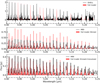 |
Fig. D.8 Same as Figure 11, but for the Gaussian line profile. |
| In the text | |
Current usage metrics show cumulative count of Article Views (full-text article views including HTML views, PDF and ePub downloads, according to the available data) and Abstracts Views on Vision4Press platform.
Data correspond to usage on the plateform after 2015. The current usage metrics is available 48-96 hours after online publication and is updated daily on week days.
Initial download of the metrics may take a while.