| Issue |
A&A
Volume 689, September 2024
|
|
|---|---|---|
| Article Number | A231 | |
| Number of page(s) | 21 | |
| Section | Planets and planetary systems | |
| DOI | https://doi.org/10.1051/0004-6361/202450078 | |
| Published online | 13 September 2024 | |
MINDS. Hydrocarbons detected by JWST/MIRI in the inner disk of Sz28 consistent with a high C/O gas-phase chemistry
1
Kapteyn Astronomical Institute, University of Groningen,
PO Box 800,
9700
AV
Groningen,
The Netherlands
2
Space Research Institute, Austrian Academy of Sciences,
Schmiedlstr. 6,
8042
Graz,
Austria
3
TU Graz, Fakultät für Mathematik, Physik und Geodäsie,
Petersgasse 16
8010
Graz,
Austria
4
Department of Astrophysics/IMAPP, Radboud University,
PO Box 9010,
6500
GL
Nijmegen,
The Netherlands
5
SRON Netherlands Institute for Space Research,
Niels Bohrweg 4,
2333
CA
Leiden,
The Netherlands
6
Leiden Observatory, Leiden University,
2300
RA
Leiden,
The Netherlands
7
Max-Planck Institut für Extraterrestrische Physik (MPE),
Giessenbachstr. 1,
85748,
Garching,
Germany
8
Institute of Astronomy, KU Leuven,
Celestijnenlaan 200D,
3001
Leuven,
Belgium
9
Max-Planck-Institut für Astronomie (MPIA),
Königstuhl 17,
69117
Heidelberg,
Germany
10
Department of Astrophysics, University of Vienna,
Türkenschanzstr. 17,
1180
Vienna,
Austria
11
ETH Zürich, Institute for Particle Physics and Astrophysics,
Wolfgang-Pauli-Str. 27,
8093
Zürich,
Switzerland
12
STAR Institute, Université de Liège,
Allée du Six Août 19c,
4000
Liège,
Belgium
13
Centro de Astrobiología (CAB), CSIC-INTA, ESAC Campus,
Camino Bajo del Castillo s/n,
28692
Villanueva de la Cañada, Madrid,
Spain
14
INAF – Osservatorio Astronomico di Capodimonte,
Salita Moiariello 16,
80131
Napoli,
Italy
15
Dublin Institute for Advanced Studies,
31 Fitzwilliam Place,
Dublin
D02 XF86,
Ireland
16
Université Paris-Saclay, CNRS, Institut d’Astrophysique Spatiale,
91405
Orsay,
France
Received:
22
March
2023
Accepted:
18
July
2024
Abstract
Context. With the advent of JWST, we are acquiring unprecedented insights into the physical and chemical structure of the inner regions of planet-forming disks where terrestrial planet formation occurs. Very low-mass stars (VLMSs) are known to have a high occurrence of the terrestrial planets orbiting them. Exploring the chemical composition of the gas in these inner disk regions can help us better understand the connection between planet-forming disks and planets.
Aims. The MIRI mid-Infrared Disk Survey (MINDS) project is a large JWST guaranteed time program whose aim is to characterise the chemistry and physical state of planet-forming and debris disks. We used the JWST-MIRI/MRS spectrum to investigate the gas and dust composition of the planet-forming disk around the VLMS Sz28 (M5.5, 0.12 M⊙).
Methods. We used the dust-fitting tool DuCK to determine the dust continuum and to place constraints on the dust composition and grain sizes. We used 0D slab models to identify and fit the molecular spectral features, which yielded estimates on the temperature, column density, and emitting area. To test our understanding of the chemistry in the disks around VLMSs, we employed the thermochemical disk model PRODIMO and investigated the reservoirs of the detected hydrocarbons. We explored how the C/O ratio affects the inner disk chemistry.
Results. JWST reveals a plethora of hydrocarbons, including CH3, CH4, C2H2, 13CCH2, C2H6, C3H4, C4H2 and C6H6 which suggests a disk with a gaseous C/O > 1. Additionally, we detect CO2, 13CO2, HCN, and HC3N. H2O and OH are absent from the spectrum. We do not detect polycyclic aromatic hydrocarbons. Photospheric stellar absorption lines of H2O and CO are identified. Notably, our radiation thermo-chemical disk models are able to produce these detected hydrocarbons in the surface layers of the disk when C/O > 1. The presence of C, C+, H, and H2 is crucial for the formation of hydrocarbons in the surface layers, and a C/O ratio larger than 1 ensures the surplus of C needed to drive this chemistry. Based on this, we predict a list of additional hydrocarbons that should also be detectable. Both amorphous and crystalline silicates (enstatite and forsterite) are present in the disk and we find grain sizes of 2 and 5 μm.
Conclusions. The disk around Sz28 is rich in hydrocarbons, and its inner regions have a high gaseous C/O ratio. In contrast, it is the first VLMS disk in the MINDS sample to show both distinctive dust features and a rich hydrocarbon chemistry. The presence of large grains indicates dust growth and evolution. Thermo-chemical disk models that employ an extended hydrocarbon chemical network together with C/O >1 are able to explain the hydrocarbon species detected in the spectrum.
Key words: astrochemistry / line: identification / protoplanetary disks / brown dwarfs / stars: low-mass / infrared: planetary systems
Corresponding author; This email address is being protected from spambots. You need JavaScript enabled to view it.
© The Authors 2024
 Open Access article, published by EDP Sciences, under the terms of the Creative Commons Attribution License (https://creativecommons.org/licenses/by/4.0), which permits unrestricted use, distribution, and reproduction in any medium, provided the original work is properly cited.
This article is published in open access under the Subscribe to Open model. This email address is being protected from spambots. You need JavaScript enabled to view it. to support open access publication.
1 Introduction
The evolution of gas and dust around very low-mass stars (VLMSs) (Liebert & Probst 1987) is only now starting to be extensively studied with new telescopes. It is important to study these objects since the occurrence of terrestrial planets around such stars is quite high. Transit observations find 2.5 ± 0.2 planets per M dwarf with radii 1–4 R⊕ and periods of <200 days (Dressing & Charbonneau 2015), and radial velocity searches have found ~1.32 planets with 1 M⊕ < Mpl sin i < 10 M⊕ and periods of <100 days (Sabotta et al. 2021; Schlecker et al. 2022). Studying the inner regions of the planet-forming disks around M-type stars sheds light on the chemistry and dust evolution in these very low-mass objects during a phase where planets are likely forming (Henning & Semenov 2013). With the advent of the James Webb Space Telescope (JWST) (Rigby et al. 2023), we can probe the warm and dense inner regions (1 au, T ~200–1000 K, n ~1010−1018 cm−3) of disks around such VLMSs with a sensitivity and spectral resolution higher than that of the Spitzer Space Telescope thus providing insight into the gas and dust properties in this region. As part of the MIRI mid-Infrared Disk Survey (MINDS) guaranteed time observations (GTO) collaboration (Henning et al. 2024; Kamp et al. 2023), the disks around the VLMS J1605321-1933159 (J160532 here in after, Tabone et al. 2023) and ISO-Chal 147 (Arabhavi et al. 2024) have been reported to have high C/O ratios in their inner regions. This inference is based on the detection of a plethora of complex hydrocarbons. No silicate features have been detected in the spectra, thus indicating dust growth and evolution since large grains tend to emit at longer wavelengths. However, there are disks around other VLMSs such as Sz114 (Xie et al. 2023) that are rich in water and only show the standard hydrocarbon C2H2, which has been previously detected with Spitzer in many T Tauri and VLMS disks (Salyk et al. 2008; Carr & Najita 2011; Pontoppidan et al. 2010; Pascucci et al. 2009). Xie et al. (2023) conclude that different initial conditions, such as a large and massive disk and potential substructures, may have kept water abundances high in the inner disk, resulting in a water-rich spectrum.
We present here the spectrum of the source Sz28 (T37 or 2MASS-J11085090-7625135) observed by the JWST-Mid InfraRed Instrument (MIRI) (Rieke et al. 2015; Wright et al. 2015, 2023) Medium-Resolution Spectrometer (MRS) (Wells et al. 2015; Argyriou et al. 2023) and investigate whether it is similar to the hydrocarbon-rich sources J160532 and ISO-Chal 147 or the water-rich source Sz114. Sz28 is a VLMS (Manara et al. 2017, M* = 0.12 M⊙, L* = 0.03 L⊙). We rescaled L* to 0.04 L⊙ based on the new distance from Gaia Data Release 3 (Galli et al. 2021). It is a member of the ~3.6 Myr old (Ratzenböck et al. 2023) Chamaeleon I star-forming region and it located at a distance of 192.2 pc (Galli et al. 2021). Its spectral type is M5.5, and it has an effective temperature of ~3060 K and an accretion rate of ~1.810−11 M⊙ yr−1 (Manara et al. 2017). An Atacama Large Millimeter/Submillimeter Array (ALMA) nondetection sets an upper limit on the disk dust mass of 0.48 M⊕ (Pascucci et al. 2016) and on the gas mass of either 0.08 MJup or 3.1 MJup, depending on the CO isotopologue method used (Long et al. 2017). Spitzer detected C2H2 line emission and revealed that the dust in this source exhibits comet-like 9.4 μm and 11.3 μm crystalline silicates, and is more processed compared to the interstellar medium (ISM) dust (Pascucci et al. 2009).
Considerable effort focused on understanding the strong features of C2H2 in disks even before JWST. Agúndez et al. (2008), Bast et al. (2013), Walsh et al. (2015), and Kanwar et al. (2024) investigated the chemistry of C2H2 in the warm, high-density gas of the inner disk and how its abundance structure changes with stellar properties and the use of different chemical networks and rate databases. Woods & Willacy (2007) and Kanwar et al. (2024) outlined the pathways to form benzene in planet-forming disks. We aim here to use thermo-chemical models to aid the interpretation of the spectrum and study the chemistry in the inner regions of the disks around VLMSs. We explore the effect of a change in the C/O elemental ratio on the hydrocarbon chemistry.
The paper is structured as follows. Section 2 describes the observations and the methods used to reduce the data, and lists the molecular detections. We then describe the determination of the dust continuum and slab model retrievals used for the subsequent quantitative analysis in Sect. 3. The non-detections and detection of dust features, along with the findings from the slab model analysis such as gas temperature, column density, and emitting area, are reported in Sec. 4. We compare our astro-chemical understanding to that of the species detected in the JWST-MIRI/MRS spectrum using thermo-chemical disk models with varying C/O ratios in Sect. 5. The comparison of Sz28 with other disks around VLMSs in terms of its gas and dust content are discussed in Sec. 6, along with the implications of our for planet formation. Finally, we summarise our findings and conclusions in Sec. 7.
2 Observations and data reduction
Sz28 was observed on August 16, 2022, at 02:06:10 for a total time of 1.02 hours in MRS mode with the JWST-MIRI instrument over the full wavelength range of 4.9–27.9 μm as part of GTO programme 1282 (PI: Th. Henning). It was observed with target acquisition in FASTR1 readout mode using a four-point dither pattern in the positive direction with an exposure time of 924 seconds in each band. The spectrum contains four channels, each with three bands.
We used version 1.11.1 (Bushouse et al. 2023) of the JWST standard Science Calibration pipeline with the CRDS context jwst_1094.pmap and VIP package (version 1.4.2; Gomez Gonzalez et al. 2017; Christiaens et al. 2023, 2024) for the reduction of the uncalibrated files. We used Detector1 of the pipeline followed by stray-light correction when either the sdither or ddither background subtraction is used. We skipped stray-light correction if we used the annulus background subtraction method (for more information see Christiaens et al. 2024). The default parameters for Spec2 were used. The VIP-based routines for bad pixel correction are used instead of the outlier detection in Spec3, as the former efficiently correct for significant spikes that would otherwise affect the extracted spectrum of the source (e.g. Perotti et al. 2023). As Sz28 had no dedicated background observation, we explored various background subtraction techniques. Initially, we used the annulus background subtraction where the median value in an annulus directly encircling the aperture used for photometry is subtracted. Subsequently, we tested the subtraction of a background proxy estimated from the rate files obtained with the four-point dither pattern, and smoothed with a median filter (sdither). Both of these methods resulted in MIRI flux levels comparable to that of Spitzer, but the spectrum was noisy. We finally used the direct pair-wise dither subtraction (ddither) to estimate the background as it led to a higher S /N in the reduced spectrum. This method results in lower flux levels than the Spitzer observations. This minor flux discrepancy is attributed to the self-subtraction between minimally overlapping point spread functions. Because of the higher S /N, this spectrum is then used for further analysis.
As there is no line-free region in the spectrum we used the JWST Exposure Time Calculator (ETC)1 to obtain an ideal estimate for the S/N as described in Temmink et al. (2024). This noise only takes into account the photon and read noise of the detector. The actual noise therefore, would be higher than we report. We used the ratio of median continuum flux level in each band and the estimated S/N as the noise level in the spectrum. These values are reported in Table 1 for bands where we detect molecular emission. The estimated noise level for the Spitzer spectrum was ~0.4 mJy (Pascucci et al. 2009) whereas the estimated noise level for the MIRI/MRS is ~0.1 mJy in channel 2. The flux differences are within the 10% Spitzer flux calibration uncertainties and 5% absolute spectro-photometric MRS uncertainty (Argyriou et al. 2023).
Figure 1 presents the identified dust and molecular features in the JWST-MIRI/MRS spectrum of Sz28 along with the Spitzer low resolution spectrum for comparison. We mote that many of the small wiggles seen in the spectrum at <20 μm are not high frequency noise but are due to individual molecular lines.
We considered a molecule as detected if we identified a Q branch above the 3σ level. For species that do not show a Q branch, multiple P- and/or R-branch lines above 3σ are required to confirm a detection. In this way, we detected the molecular emission bands listed in Table 2. Several clear features indicated by red questions marks on the spectrum (Fig. 1) remain so far unidentified. In the following, we detail the quantitative methods used to analyse the spectrum further.
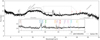 |
Fig. 1 JWST-MIRI/MRS spectrum of Sz28. The detected molecular species and the dust features are labelled. The spectrum from Spitzer is depicted in grey. The red question mark (?) indicates the unidentified spectral features and the red horizontal lines show their wavelength range. The Q branches of the molecules are shown as solid lines along with their identified isotopologues, if any, as dotted lines. |
S/Ns provided by ETC along with the median continuum flux in each band where molecules are detected.
3 Analysis methods
3.1 Continuum subtraction
To identify the molecules in the spectrum, we needed to determine a reliable dust continuum. In contrast with other VLMSs, we observe the silicate dust feature at 10 μm and an unusual, weak 16 μm feature. We first assumed the lower envelope of the spectrum as the dust continuum. Based on the residuals of the initial fitting of the molecular features, the presence of a molecular pseudo-continuum was found similar to Arabhavi et al. (2024).
To subsequently better guide our continuum placement and explain the ~16 μm feature we employed the dust retrieval code (Dust Continuum Kit; DuCK) explained in detail in Kaeufer et al. (2024) and Jang et al. (in prep.), using a similar approach as Juhász et al. (2010). It is a 1D code that uses three components to explain the dust emission: a rim, optically thick midplane and optically thin surface layer and uses Bayesian analysis to fit the observations. The code uses a library of dust species. For crystalline dust, we used enstatite (Jaeger et al. 1998), and forsterite (Servoin & Piriou 1973). For amorphous dust, we used silica (Spitzer & Kleinman 1960), silicates with pyroxene (Dorschner et al. 1995) and olivine (Henning & Stognienko 1996) stoichiometry. We then fitted the dust features based on these dust absorption coefficients using a range of grain sizes (0.1–5 μm). The Gaussian random field method is used to calculate the Q curves for the dust species (Jang et al., in prep.; Min et al. 2007).
When using the entire spectrum, we find that the dominant dust species varies between the shorter and longer wavelengths. This is because the code gives more weight to shorter wavelengths resulting in a fit that failed to capture the overall shape of the dust continuum at longer wavelengths. Consequently, this makes it difficult to recover the peculiar feature at 16 μm. To address this issue, we opted to divide the spectrum into two wavelength ranges, short (4.9–15 μm) and long (15–22 μm), and use the dust model to fit them separately. Fitting the spectrum in such a way, produces a forsterite feature around 16 μm after taking into account the molecular emission contribution to the continuum. The peak of the observed feature is slightly blue-shifted compared to this dust model fit. However, this shift could be attributed to imperfect opacity curves. This feature could thus be explained by four different scenarios: different dust composition, imperfect opacity curves, a molecular pseudo-continuum or a combination thereof.
We deviated from the continuum found using the dust retrieval code based on the residuals that are due to molecular features. We also excluded the data longwards of 22 μm as it is noisy and spurious due to lack of signal. As the dust continuum was overestimating the dust strength at various wavelengths, we selected certain points informed by the dust fit as shown in Fig. A.2. We then used a cubic-spline fit function (Dyer & Dyer 2001, CubicSpline) to interpolate the continuum which is now only informed by the dust-fit models, as shown in Fig. A.2, and is therefore not the direct output of the dust retrieval code (see Appendix A for more details).
Molecular detections in Sz28.
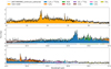 |
Fig. 2 Top panel: continuum-subtracted JWST-MIRI/MRS spectrum of Sz28 showing the total model (addition of slabs of all the detected molecules) in the wavelength region 12–17 μm. Bottom two panels: individual contribution of the slab models for the detected molecular species. The slab model fits are performed over the wavelength window shown at the bottom of the panel as a straight line for a molecule in their corresponding colour. The slab parameters of the spectrum of not well-constrained molecules can be found in Table B.1. |
3.2 0D modelling
We used 0D slab models for the identification of the molecules and to estimate the gas temperature (T), column density (N) and the emitting radius (Rem) consistent with the observed molecular emissions. T is varied in intervals of 25 K from 25 K to 1500 K. N in log-scale is varied from 1014 to 10245 cm−2 in intervals of ![Mathematical equation: $\[0.1 \overline{6}\]$](/articles/aa/full_html/2024/09/aa50078-24/aa50078-24-eq1.png) dex. The emitting area in log-scale is varied between 0.01 and 100 au. We used ProDiMo (Woitke et al. 2009; Woitke et al. 2016) and the prodimopy (v2.1.4) Python package for generating slab models and performing χ2 fits, respectively, as explained in Arabhavi et al. (2024). The spectroscopic data are taken from HITRAN (Gordon et al. 2022), Delahaye et al. (2021), (C3H4, C6H6) and Helmich (1996), (CH3). For C3H4 and C6H6, we used the partition functions, Einstein coefficients and degeneracies from Arabhavi et al. (2024). The slab models are convolved to the MIRI/MRS resolving power (R = 2500 for channel 3 and 3500 for channel 1) and resampled to the JWST-MIRI/MRS wavelength grid using the Python package SpectRes (Carnall 2017). We use the noise estimate described in Sect. 2. For C2H2 and CO2 whose emission spans bands 3A and 3B, and 3B and 3C, respectively, we calculated the final noise (σ) as:
dex. The emitting area in log-scale is varied between 0.01 and 100 au. We used ProDiMo (Woitke et al. 2009; Woitke et al. 2016) and the prodimopy (v2.1.4) Python package for generating slab models and performing χ2 fits, respectively, as explained in Arabhavi et al. (2024). The spectroscopic data are taken from HITRAN (Gordon et al. 2022), Delahaye et al. (2021), (C3H4, C6H6) and Helmich (1996), (CH3). For C3H4 and C6H6, we used the partition functions, Einstein coefficients and degeneracies from Arabhavi et al. (2024). The slab models are convolved to the MIRI/MRS resolving power (R = 2500 for channel 3 and 3500 for channel 1) and resampled to the JWST-MIRI/MRS wavelength grid using the Python package SpectRes (Carnall 2017). We use the noise estimate described in Sect. 2. For C2H2 and CO2 whose emission spans bands 3A and 3B, and 3B and 3C, respectively, we calculated the final noise (σ) as:
![Mathematical equation: $\[\sigma_{\mathrm{C}_2 \mathrm{H}_2}=\frac{W_{3 \mathrm{A}} \cdot \sigma_{3 \mathrm{A}}+W_{3 \mathrm{B}} \cdot \sigma_{3 \mathrm{B}}}{W_{3 \mathrm{A}}+W_{3 B}}\]$](/articles/aa/full_html/2024/09/aa50078-24/aa50078-24-eq2.png) (1)
(1)
![Mathematical equation: $\[\sigma_{\mathrm{CO}_2}=\frac{W_{3 \mathrm{B}} \cdot \sigma_{3 \mathrm{B}}+W_{3 \mathrm{C}} \cdot \sigma_{3 \mathrm{C}}}{W_{3 B}+W_{3 C}}\]$](/articles/aa/full_html/2024/09/aa50078-24/aa50078-24-eq3.png) (2)
(2)
where W is the number of data points used to calculate χ2 from each band (Temmink et al. 2024). We use the resulting continuum-subtracted spectrum (see Sect. 3.1) to fit the slab models for one molecule or group of molecules at a time and subtract this best-fit slab from the spectrum. The residual spectrum is then used for fitting the subsequent molecules, again one at a time as described below. We calculate the χ2 between the continuum-subtracted observed spectrum and the convolved and re-sampled slab modelled spectrum (Kamp et al. 2023; Grant et al. 2023). The mask used in the χ2 determination for each molecule is defined over the wavelength region that has the least contamination from other molecules (see Fig. 2).
We did not fit bands 1A (4.9–5.74 μm) and 1B (5.66–6.63 μm) as they are dominated by the stellar spectrum (see Fig. A.1). The low resolution stellar model spectrum obtained from PHOENIX (Brott & Hauschildt 2005) using the stellar parameters (Sect. 1) is not good enough to correct for this; more work is required to obtain a good fitting high resolution stellar spectrum. We also did not fit any molecular emission features between 8.9 and 11.8 μm as they are hard to disentangle from the dust emission.
Here we explain our fitting methodology (especially the order and grouping of molecules) in more detail as the spectrum shows blending of molecular emission at various wavelengths. We find channel 3B in the wavelength range 13.0–14.5 μm to be dominated by the ν5 mode of C2H2. The slab models for C2H2 include its isotopologue 13CCH2 in the ratio 1:35 (Woods & Willacy 2009) and are thus treated as a ‘single’ species. The spectroscopic data for 13CCH2 are available only for the lowest ν5 (1–0) band. We used optically thick (N>1019 cm−2) and thin (N<1019 cm−2) slabs of C2H2 to fit the line emission in this band and treated it as fitting two species simultaneously (thus the free parameters are N1 × T1 × Rem1 × N2 × T2 × Rem2 where 1 and 2 correspond to the optically thick and thin components, see Arabhavi et al. 2024). The χ2 was evaluated in the wavelength window 13.00–13.71 μm. We observed the Q branch peaks of 13CCH2 at 13.69 and 13.73 μm but purposely defined the fitting window excluding the latter wavelength as it leads to over-prediction of the free parameters due to the incomplete spectroscopic data for 13CCH2. We then subtracted this bestfit slab model (thick and thin components of C2H2) from the continuum-subtracted spectrum. Next, we performed the fit for C6H6 in the wavelength region 14.3–15.27 μm, because this is now the dominant feature in the residual spectrum. Again, the resulting best-fit slab for C6H6 was subtracted from the spectrum. In a next step, the new residual spectrum was then used to fit the remaining molecules one by one in the following order HC3N−CO2−HCN−C2H6 (only for confirming the detection)-(C4H2 + C3H4; fitted together). The wavelength windows over which the χ2 is evaluated to determine best fits are performed are shown in Fig. 2. We did not fit CH3 as we have incomplete spectroscopic data comprising of only a single band for this molecule; we used this only for confirming the detection. In band 1C, 6.5–8.2 μm, we only have a clear detection of CH4 (see Fig. 3). We did not fit the species since the presence of absorption lines suggests there is likely a stellar contribution, which we cannot easily correct for. Figure 3 shows a slab model visually matched to the data of CH4 to depict its detection.
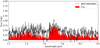 |
Fig. 3 Slab model for CH4 shown in red along with the zoomed-in JWST-MIRI/MRS spectrum of Sz28. The parameters from the 0D slab models for the represented slab can be found in Table B.1. |
4 Results
The subsequent paragraphs describe more quantitatively the dust and molecular content that we find in the JWST-MIRI/MRS spectrum.
Best-fit slab model parameters for the molecules detected in Sz28.
4.1 Dust composition and sizes
The shape of the continuum indicates the presence of silicate dust. The shape and strength of the silicate feature is determined by the grain size and composition (Henning 2010). Based on the dust fitting that decomposes the spectrum into emission from dust species, we identify the 9.2 μm feature of SiO2, the 11.3 and 19.3 μm features of forsterite, and the 9.4, 9.9, and 18.2 μm features of enstatite. Thus, the dust composition comprises amorphous and crystalline silicates, which indicates that the dust in the disk has undergone thermal processing. The mass fraction of crystalline silicates is ~20% and the rest are amorphous silicates. The ratio of the two crystalline dust species enstatite and forsterite change between the wavelength regions. Forsterite is more abundant than enstatite in the longer wavelength region (18.8% and 3%, respectively), whereas in the shorter wavelength region, the abundances of forsterite and enstatite are similar (9.4% and 7.5%, respectively). For amorphous silicates, the dust model indicates quite large grains, typically 5 μm, and for forsterite, we find both large grains ~5 μm and slightly smaller grain sizes, typically 2 μm. The dust models predict systematically smaller grain sizes ~2–3 μm for enstatite.
4.2 Gas molecular content
Figure 2 shows the resulting continuum-subtracted spectrum and the 0D slab model fits for all the detected species. We provide the values of T, N and Rem consistent with these molecular emission in Table 3 along with 1 σ uncertainties. We note that there is a degeneracy between the gas temperature T and the column density N for the same species, which is evident from the χ2 plots (see Fig. B.1). The S/N of the spectrum is low and subsequently, many fits are not well constrained.
The slab model fitting indicates that the optically thick C2H2 has high column densities giving rise to a molecular pseudo-continuum. This optically thick emission originates from a smaller emitting area compared to the optically thin emission similar to the findings of Tabone et al. (2023) and Arabhavi et al. (2024). C6H6 has its temperature constrained between 110 K and 550 K with column densities ranging between 1017.5 and 1019.5 cm2.
The temperatures and column densities of the molecules CH3, CH4, HCN, HC3N, CO2, and C2H6 are poorly constrained, and therefore, we refrain from providing ‘best-fit parameters’ in Table 3. The parameters describing the slabs used to identify these species in Fig. 2 are listed in Table B.1. CH3 is not fitted as we have incomplete spectroscopic data. HCN is detected, but its emission is blended with C2H2 and therefore it is hard to constrain its parameters. The emission of HC3N and CO2 overlaps with the P branch of C6H6 making it difficult to provide best-fit values. We find that CO2 is cold compared to many of the other molecules with temperatures between 100 K and 250 K and column densities greater than 1018.5 cm−2. This low temperature is driven by the narrow shape and the peak positions of the Q branches of the main and hot 12CO2 bands and the 13CO2 band (see Fig. C.1). HC3N has a column density lower than 1021 cm−2 and the temperature varies between 50 K and 690 K as evident from the χ2 map in Fig. B.1. C2H6 is also poorly constrained in our analysis. Its spectral signature coincides with the region where the spectral leak correction was applied (at 12.2 μm Wells et al. 2015). Unfortunately, the 1.11.1 version of the standard pipeline did not yet correct for this leak.
There are still many unidentified spectral features longwards of 16.5 μm some of which are indicated with a question mark in Fig. 1. In addition, we were not able to identify the 12.844 μm broad feature.
We do not detect any polycyclic aromatic hydrocarbon (PAH) emission features, OH, NH3, atomic or molecular hydrogen emission or metal fine-structure lines given the current quality of the spectrum. We do not detect H2O or CO emission from the disk. This is because the short wavelength region up to 6.5 μm is dominated by the stellar spectrum as seen in Fig. A.1. The overall shape of the PHOENIX stellar spectrum closely matches with the observed Sz28 MIRI/MRS spectrum, although the stellar model has a lower spectral resolution than MIRI/MRS. We clearly detect H2O and CO stellar absorption lines similar to the case of ISO-Chal 147 (Arabhavi et al. 2024, Fig. S6). To search for the potential presence of H2O or CO emission from the disk, we thus first require high resolution photospheric stellar models to disentangle the stellar and disk contribution at the short wavelengths. This is outside the scope of this paper.
The richness in hydrocarbon features and non-detection of oxygen-bearing molecules (except CO2) point towards an inner disk with an elemental ratio C/O > 1. The absence of the [Ne II] line is in agreement with the upper limit of stellar X-rays log(LX/erg s−1) ~28.9 (Güdel et al. 2010). The nondetection of H2O, OH and CO does not necessarily imply their absence, but rather puts an upper limit to their column densities and/or emitting areas given the estimated noise level (0.1 mJy).
As explained above, in many cases T, N and Rem for molecules are not well-constrained. However, all these molecules except CO2 share some common parameter space indicating that they might be sharing a single emitting reservoir. CO2 is the only molecule with temperatures as low as 100–250 K based on the χ2 maps, indicating that CO2 could have a different emitting region. We also followed the approach of Tabone et al. (2023) to fit species using the emitting area of the optically thick or thin component of C2H2 to minimise uncertainties and better constrain parameters T and N. However, using either of the emitting areas, we were not able to explain the flux levels observed in the spectrum for other molecules such as C6H6. Simultaneously fitting the dust and molecules in a wavelength region and allowing for radial density and/or temperature gradients may constrain the parameter space better, but is outside the scope of this paper. It requires advanced fitting strategies such as CLIcK (Liu et al. 2019) or DuCKLinG (Kaeufer et al. 2024).
5 Hydrocarbon chemistry in disks around VLMSs
The above analysis has shown that the gas in the inner disk is very rich in hydrocarbons, leaving open the question whether our chemical networks can adequately describe the formation of all these hydrocarbons in such warm, high-density disk environments. The 0D slab models used in the Sec. 3.2 do not consider temperature gradients, dust opacity, the gas heating and cooling balance, chemistry, and are therefore not suited to discuss and understand the chemical pathways at play. To investigate the above question, we used radiation thermochemical disk models. Our primary objective here is not to fit the observed spectrum, but to test whether the hydrocarbon molecules we detect are consistent with our understanding of the chemistry in these environments (high-density inner disks and high C/O).
5.1 Thermo-chemical modelling
We used the radiation thermo-chemical code PRODIMO to simulate a typical disk around a VLMS. This is a 2D code that can model the physical and chemical structure of the disk selfconsistently (Woitke et al. 2016). It calculates the dust temperature structure from dust radiative transfer and the gas temperature by balancing the gas heating and cooling processes. Greenwood et al. (2017) presented a brown dwarf PRODIMO disk model with stellar properties similar to those of Sz28. We adopted the same disk model and change the stellar parameters to those of Sz28. A detailed list of the disk model parameters can be found in Table D.1. To have a gradual buildup in the surface density in the inner regions, we used a soft inner rim as explained in Woitke et al. (2024). We define the surface density ∑(r) as
![Mathematical equation: $\[\Sigma(r) \propto \exp \left[-\left(\frac{R_{\text {soft }}}{r}\right)^s\right] r^{-\epsilon} \exp \left[-\left(\frac{r}{R_{\text {tap }}}\right)^{2-\epsilon}\right]\]$](/articles/aa/full_html/2024/09/aa50078-24/aa50078-24-eq20.png) (3)
(3)
where Rtap is the tapering-off radius,
![Mathematical equation: $\[R_{\text {soft }}=\text { raduc } \times R_{\text {in }}\]$](/articles/aa/full_html/2024/09/aa50078-24/aa50078-24-eq21.png) (4)
(4)
and
![Mathematical equation: $\[s=\frac{\ln [\ln (1 / \text {reduc})]}{\ln (\text {raduc})} \text {. }\]$](/articles/aa/full_html/2024/09/aa50078-24/aa50078-24-eq22.png) (5)
(5)
The power law exponent ϵ is 1. The raduc parameter defines the radius up to which the density is gradually building up in units of inner disk radius Rin and is chosen to be 1.15. The reduc parameter determines the reduction of the column density around the inner rim and is chosen to be 10−7. We used the extended hydrocarbon chemical network added to the large DIANA chemical network (Kamp et al. 2017; Kanwar et al. 2024) and steady state chemistry. The largest hydrocarbon species that this chemical network can form is C8H5+. The reactions are primarily taken from UMIST2012 (McElroy et al. 2013). In addition, the network takes into account three body and thermal decomposition reactions. The elemental abundances are the low-ISM values taken from Kamp et al. (2017). The gas and dust temperature and the UV radiation field calculated from detailed 2D radiative transfer (in units of the Draine field) of both the models are shown in Fig. D.1.
We used two models to compare our chemical understanding to the molecular detections in our JWST mid-IR spectra of disks around VLMSs. One model has the canonical C/O elemental ratio of 0.45 (Anders & Grevesse 1989). The second model has a lower oxygen abundance, resulting in a C/O of 2. In both models, we kept the gas temperature structure fixed to that of the canonical model. This approach allowed us to isolate the effects of the change in elemental abundance on the species abundances from the effect of gas temperature as the chemistry and gas temperature are naturally intertwined.
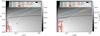 |
Fig. 4 Abundance contours corresponding to 10% of the maximum abundance of the hydrocarbons detected in disks around VLMSs in the canonical and enhanced model with C/O of 0.45 and 2.0, respectively. The white contours correspond to the gas temperatures of 140 K and 475 K. The Aυ =1 mag contour is shown in black. |
5.2 Hydrocarbon chemistry
The hydrocarbon chemistry has been recently revisited in the context of disks around T Tauri stars (Kanwar et al. 2024). They find that the dissociation of CO unlocks C (UV radiation) or C+ (X-rays or cosmic rays). This carbon can then abstract H from H2 or combine with another C to form hydrocarbons in the disk surfaces. However, in cases where oxygen is depleted, there is unblocked C already present to form hydrocarbons. The main neutral-neutral and ion-molecule pathways of formation and destruction for C2H2 and C6H6 in a disk around T Tauri star are outlined in Kanwar et al. (2024). These pathways agree with Walsh et al. (2015) for C2H2 and McEwan et al. (1999) for C6H6. While Woods & Willacy (2007) find that the ion-neutral pathway of C3H4 reacting with its own ion a major reaction leading to C6H6 via C6H7+, Kanwar et al. (2024) find the reaction of C6H5+ with H2 via C6H7+ to dominate the C6H6 formation.
We used the above described model of a disk around a VLMS to investigate whether the gas phase formation and destruction pathways remain the same as for the T Tauri disk and whether they depend on the C/O ratio. Figure 4 shows where the observationally detected hydrocarbons reside in the disk for the canonical and enhanced C/O elemental ratio. The abundance contours outline a value of 10% of their respective maximum abundance. Table D.2 lists the maximum abundance, maximum total column density and total column density at 0.1 au of these species in both models. We note that the maximum values are similar in the two models, but the spatial region over which a species exhibits these corresponding values radially and vertically expands in the enhanced C/O model. We note that the molecular emission in the mid-IR spectrum is in fact limited by the dust continuum, and so does not reflect the full molecular column density (see Fig. D.1). This model is not tailored towards Sz28 specifically as we have too few constraints on the physical disk parameters. Thus, deep integration ALMA observations are required to constrain these parameters and improve the chemical understanding extracted from such thermo-chemical disk models.
In the model with the canonical C/O elemental ratio, the detected hydrocarbon molecules are concentrated in a radially narrow, but vertically extended area in the inner 0.1 au, close to the disk midplane. Increasing the C/O ratio to 2, the chemistry shifts to a carbon-dominated chemistry. This results in increased abundances by ~4 to ~10 orders of magnitude in the surface layers and in the inner disk, respectively (see Figs. D.3 and D.4).
We next analysed whether there are new chemical pathways in both models that become active and lead to such complex hydrocarbons; we used C2H2 and C6H6 as proxies to be able to compare with our earlier work on T Tauri disks (Kanwar et al. 2024). We used the same approach here and analysed the grid point r = 0.248 au and z = 0.042 au lying in the line emitting region of C2H2 to study the chemical pathways of C2H2 and C6H6. This point is characterised by the following condition: Tgas = 270 K and ![Mathematical equation: $\[T_{\text {dust }}=230 \mathrm{~K}, n_{\langle\mathrm{H}\rangle}=6.4 \times 10^{10} \mathrm{~cm}^{-3} \text {, }A_{\mathrm{V}}^{v e r}=0.018\]$](/articles/aa/full_html/2024/09/aa50078-24/aa50078-24-eq23.png) , vertical visual extinction,
, vertical visual extinction, ![Mathematical equation: $\[A_{\mathrm{V}}^{\mathrm{rad}}=1.1\]$](/articles/aa/full_html/2024/09/aa50078-24/aa50078-24-eq24.png) , radial visual extinction. We find that the chemical pathways leading to C2H2 in the canonical model (disk around a VLMS, C/O=0.45) are similar to the findings of Kanwar et al. (2024) (disk around a T Tauri star, C/O=0.45). We find that the reaction
, radial visual extinction. We find that the chemical pathways leading to C2H2 in the canonical model (disk around a VLMS, C/O=0.45) are similar to the findings of Kanwar et al. (2024) (disk around a T Tauri star, C/O=0.45). We find that the reaction
![Mathematical equation: $\[\mathrm{C}_2 \mathrm{H}+\mathrm{H}_2 \rightarrow \mathrm{C}_2 \mathrm{H}_2+\mathrm{H}\]$](/articles/aa/full_html/2024/09/aa50078-24/aa50078-24-eq25.png) (6)
(6)
contributes ~91% to the formation of C2H2 in the canonical C/O model and ~96% in the model with enhanced C/O. The photodissociation of C2H2 to C2H contributes ~71% in the model with canonical C/O and ~37% to the destruction of C2H2 in the carbon enhanced model. The chemistry in the canonical C/O model is driven by oxygen, but when this element is depleted, other reactions having carbon as one of the reactants become more important for the formation of C2H2 (see Appendix D for more details). A high C/O ratio leads to high abundances of hydrocarbons in the disk surface layers and those destroy H2 through H abstraction. This leads to the H/H2 transition being pushed slightly deeper into the disk compared to the canonical C/O model (see Fig. D.2 and Appendix D for more details).
C6H6 is formed in both VLMS disk models primarily via
![Mathematical equation: $\[\mathrm{C}_6 \mathrm{H}_7^{~+}+\mathrm{e}^{-} \rightarrow \mathrm{C}_6 \mathrm{H}_6+\mathrm{H}.\]$](/articles/aa/full_html/2024/09/aa50078-24/aa50078-24-eq26.png) (7)
(7)
It is the only formation reaction available in UMIST2012. C6H7+ is formed via C6H5+ in both models similar to the findings of Kanwar et al. (2024). C6H5+ is formed via radiative association between C2H2 and C4H3+ in both models. The abundance of C2H2 increases in the model with enhanced C/O, which subsequently results in an increased abundance of C6H6. The reactions contributing to the destruction of C6H6 shuffle in importance because of the increased C2H2 abundance. Appendix D provides an in-depth analysis.
In general, we find that the dominant formation and destruction pathways do not change for these two species with increasing C/O. The reaction rates increase in the model with an enhanced C/O ratio and we find a shift in the relative importance of the pathways. We did not find any ‘new’ pathways that become active only when increasing the C/O ratio. However, we note that the details of the pathways depend on the location in the disk due to the gas temperature and densities changing throughout the disk.
This generic model for a disk around a VLMS also predicts the following hydrocarbons to be co-spatial with the detected hydrocarbons: C2, C2H, C3, CH2CCH and both cyclic and linear isotopomers of C3H2, C5H2, CH3C4H, C6 and C6H2. Unfortunately, none of these hydrocarbons have ro-vibrational mid-IR spectra in the HITRAN (Gordon et al. 2022) or GEISA (Delahaye et al. 2021) databases. However, the pure rotational lines of the two species C2H and c-C3H2 have been detected in the millimetre and sub-millimetre wavelength regions with ALMA in disks around T Tauri stars, albeit at much lower column densities (Qi et al. 2013; Bergin et al. 2016). These molecules may also have observable ro-vibrational lines. Theoretical calculations along with laboratory spectroscopic measurements are needed to search for these molecules in the mid-IR spectra.
6 Discussion
6.1 Dust evolution
We find that Sz28 has clear distinctive dust features. The almost flat 10 μm silicate feature indicates significant grain growth consistent with the fast dust evolution (1–3 Myr) in VLMSs as shown in Apai et al. (2005). The large grain sizes obtained from our dust models (see Sec. 4) also align with the grain growth scenario. The grains seem systematically larger than for T Tauri disks, where winds could explain the depletion of sub-micron-sized grains (Olofsson et al. 2009; Oliveira et al. 2011).
Apai et al. (2005) studied the dust processing in disks around brown dwarfs by studying the link between the strength and shape of silicate features. They analysed the flux ratio at 11.3 and 9.8 μm against the peak flux over continuum ratio. We get a value of 1 for the former and 1.4 for the latter. This places Sz28 in Apai et al. (2005, Fig. 2) in a region where the correlation between weak dust feature and crystalline silicates contribution is nonlinear meaning the crystalline silicate features become dominant. The crystalline mass fraction of Sz28 (~20%) is consistent with the findings of Apai et al. (2005) for VLMSs (9–48%). The presence of the crystalline dust features indicates thermal processing of the dust (Pascucci et al. 2009). Following Kessler-Silacci et al. (2007), the silicate emission region scales with the stellar luminosity as ![Mathematical equation: $\[L_{\star}^{0.56}\]$](/articles/aa/full_html/2024/09/aa50078-24/aa50078-24-eq27.png) , suggesting that we probed the very inner regions of these VLMS disks, ~0.05 au. Crystallisation of dust can occur by thermal annealing at ~700 K or by gas-phase condensation of silicates at high temperatures (Fabian et al. 2000). Such temperatures can exist in the inner disk. These crystalline silicates can subsequently be redistributed in the disk by radial drift, diffusion or vertical turbulence (Jang et al. 2024).
, suggesting that we probed the very inner regions of these VLMS disks, ~0.05 au. Crystallisation of dust can occur by thermal annealing at ~700 K or by gas-phase condensation of silicates at high temperatures (Fabian et al. 2000). Such temperatures can exist in the inner disk. These crystalline silicates can subsequently be redistributed in the disk by radial drift, diffusion or vertical turbulence (Jang et al. 2024).
Sz28 is not detected with ALMA in the continuum contrary to Sz114, and therefore is probably compact in dust. This could be due to an efficient radial drift, which is known to be stronger in disks around VLMSs (see Pinilla 2022). There is observational evidence of such strong radial drifts in bright disks around VLMSs (Kurtovic et al. 2021). The high C/O ratio in the inner regions of the disk around Sz28 could indicate that significant radial drift has taken place (Mah et al. 2023). Mah et al. (2023) found that short viscous timescales and close-in ice lines in VLMSs result in a high gaseous C/O after 2 Myr. Mah et al. (2024) take into account the substructures also. They introduce a gap at 10 au beyond the CO2 ice line in their model at different times ranging from 0 to 1 Myr. They find that for low viscosities (< 10−4), the inner disk can remain abundant in water for long periods of time (at least 5 Myrs) irrespective of the depth of the gap and when it is formed (see Mah et al. 2024, Fig. D.2, top two panels). This may explain water-rich sources such as Sz114. However, with a viscosity of 3×10⁻⁴, the inner disk can remain water-rich for up to 2 Myrs and then begins to transition to a high C/O ratio.
Sz28 shows large grain sizes and some fraction of crystalline dust (based on the analysis of the Si feature in Sec. 4.1). The visual inspection of the silicate feature shows that Sz114 may have low crystalline dust fraction compared to Sz28; additionally, the spectral energy distribution slope beyond 10 μm is rising in the former, whereas it is flat in the latter. This would imply that Sz114 could have more ‘primitive’ dust, indicating an earlier phase of evolution compared to Sz28. If the grains evolve as stated above, the presence of silicate features in Sz28 could indicate an intermediate phase of evolution while ISO-Chal 147 and J160532 are representative of later phases of evolution because they lack evidence of a silicate feature (grain sizes grown beyond ~5 μm or dust entirely depleted).
6.2 Gas content of VLMS disks
Sz28 shows a larger variety of hydrocarbons than J160532 whose spectrum is dominated by C2H2. All the molecules detected in ISO-Chal 147 are also detected in Sz28 except for C2H4. Similar to ISO-Chal 147, Sz28 also shows the ‘magic’2 molecule composition. Similar to the other two sources, C2H2 also forms a molecular pseudo-continuum in Sz28 along with the presence of the isotopologue 13CCH2. Due to the incompleteness of the spectroscopic data for 13CCH2 and the noise level of the MIRI/MRS spectrum of this source, we cannot reliably determine the isotopic ratio. The molecules in common in the three disks are C2H2, C4H2, C6H6, CO2 and 13CO2. None of the three disks shows PAHs or H2O or OH emission. This suggests a high C/O ratio in the inner regions of all three disks. This is contrary to Sz114 that shows clear water and CO emission, likely indicating a low C/O ratio.
In Sz28, we find high column densities of hydrocarbons even in the presence of silicate features. Neither ISO-Chal 147 now J160532 show any dust features, and both have high column densities of hydrocarbons. Thus, the absence of dust features does not necessarily imply detecting more hydrocarbons because we probed deeper into the disk.
All three sources show CO2 and strong C2H2 emission lines together; this may be hard to reconcile with an overall high C/O ratio, where O would be predominantly bound in CO. Woitke et al. (2018) show that the emission of CO2 is mainly coming from the tenuous surface layer rather than the inner reservoir. This may mean that CO2 does not necessarily need a high abundance to emit in the mid-IR (see Fig. D.6).
Tabone et al. (2023) invoke the presence of a gap that holds back O-rich icy grains to explain the high C/O in the inner disk. If we follow this idea, then it means that the outer disk could still have a normal C/O ratio and give rise to the CO2 emission. Such a scenario could explain why we systematically detect both species in VLMSs. However, in that case, the CO2 emission should be systematically cooler than the hydrocarbons, but the degeneracies on T and N in the J160532 spectrum limits our conclusions (Tabone et al. 2023). Clearly, more work is needed to understand the simultaneous presence of strong C2H2 and CO2 emission in these disk spectra.
All the three disks differ from the water-rich disk around the VLMS Sz114. Xie et al. (2023) argue that the young disk has a supply of water due to the efficient radial drift of icy pebbles beyond the snow line. This disk may represent conditions that are a precursor to Sz28. Despite having similar spectral types, these objects show differences in dust content and molecular complexity and form the starting point of a deeper investigation using a larger sample of these objects.
The steady state gas-phase chemistry with an extended chemical network is able to form the species detected in the surface layers of disks around VLMSs with a C/O> 1 (depleted oxygen). This increase in the C/O ratio in the disk can be caused by various factors, for example the close-in ice lines and the short viscous timescales (~2 Myr) of disks around VLMSs (Mah et al. 2023), the destruction of carbon grains (Tabone et al. 2023; Arabhavi et al. 2024) or transport processes carrying O-rich ices on grains inside the snow line leading to O-rich gas that then gets accreted onto the star leaving behind a high C/O ratio gas (Arabhavi et al. 2024). Based on the models, the timescales for the chemistry are ~1 yr, which means that the chemistry can adjust to the dynamic disk evolution that operates on viscous and grain drift timescales. Hence, we could conclude from this that the chemistry adjusts very quickly to any change in C/O ratio in the gas caused by any of the processes mentioned and our chemical network is adequate in describing the gas phase processes that occur therein.
Properties of the VLMS disks observed with JWST-MIRI/MRS.
6.3 Radiation field environment
Table 4 lists a number of key properties of the four VLMSs that have been analysed so far. The estimated upper limit on the X-ray luminosity of Sz28 along with the absence of the [Ne II] and [Ne III] lines in the spectrum indicate a weak X-ray radiation field and/or the absence of high-velocity jets. This is similar to the other hydrocarbon-rich disks, J160532 and ISO-Chal 147. However, it is in contrast to Sz114 which has a relatively high X-ray luminosity (see Table 4) and where the [Ne II] line indicates the presence of jets (Xie et al. 2023). It also has a higher ![Mathematical equation: $\[\dot{M}_{\mathrm{acc}}\]$](/articles/aa/full_html/2024/09/aa50078-24/aa50078-24-eq29.png) and this is consistent with detection of H2 lines, similar to J160532. The low Lacc in Sz28 and ISO-Chal 147, is consistent with the non-detections of HI and/or H2 emission in both sources. J160532 on the other hand has stronger Lacc and indeed shows strong HI and H2 lines (Franceschi et al. 2024).
and this is consistent with detection of H2 lines, similar to J160532. The low Lacc in Sz28 and ISO-Chal 147, is consistent with the non-detections of HI and/or H2 emission in both sources. J160532 on the other hand has stronger Lacc and indeed shows strong HI and H2 lines (Franceschi et al. 2024).
The low UV field and the presence of dust in Sz28 also indicate that the carbon enrichment via photo-destruction (Arabhavi et al. 2024) is less probable. The non-detection of PAHs can be attributed to either a lack of excitation due to the weak UV field or their absence in the disk.
6.4 Evolutionary age
Taking the stellar luminosity as a proxy for the age, Xie et al. (2023) argue that Sz114 is younger than J160532 and this could explain the low C/O ratio in the former following the disk evolution models from Mah et al. (2023). Following this line of argument, the luminosity of ISO-Chal 147 being the lowest of the four indicates that it could be the oldest source. This would also be consistent with the conclusion drawn from the 10 μm dust emission feature (see Sect. 6.1).
However, when assuming the ages of the star-forming regions (Table 4) as a proxy for the individual sources, we would conclude that Sz28 and ISO-Chal 147 are of the same age, followed by Sz114 and J160532 would be the oldest one. Hence, this leaves us with an inconsistent picture concerning the evolutionary sequence of these four sources and a larger sample of VLMSs is required to understand what drives the differences seen in the spectra (Arabhavi et al., in prep.).
6.5 Implications for planet formation
Terrestrial planets form in dense, warm, inner regions of disks around these young stars. With JWST, we probed these regions around Sz28 and detect plenty of hydrocarbons, which implies a high gaseous C/O ratio. The composition of the planets is influenced by their formation environment (Mollière et al. 2022; Öberg et al. 2011), in this case, a high gaseous C/O ratio environment.
If the high C/O ratio in the gas reflects a similar C/O in the refractory material of the dust, it can then lead to future planets that have a layer of graphite on top of the silicate mantle (Hakim et al. 2019). However, if the dust is complimentary to the gas and thus has a low C/O ratio, it can instead lead to the formation of terrestrial planets that are carbon-poor like Earth.
The short wavelengths of the spectrum (below 6.5 μm) are dominated by the stellar photosphere which shows the presence of O-bearing species like CO and H2O that hints at a low stellar C/O ratio. However, planet formation models that use observed stellar abundances show that the stellar photospheric C/O ratio is likely not correlated with the terrestrial planet’s C/O (Thiabaud et al. 2015).
Protoplanets formed around VLMSs can grow via pebble accretion (Liu et al. 2020). Barrado y Navascués & Martín (2003); Barrado y Navascués et al. (2007) and Luhman & Mamajek (2012) suggested that the apparent lifetime of disks are long (~10 Myr). If the protoplanet grows sufficiently in size prior to the disk dispersal, it can hold its primordial atmosphere, which would be dominated by hydrogen and helium. This atmosphere can reflect the enrichment in volatiles (C, O, N, and P) beyond H and He in the inner disk (Krijt et al. 2022). In hot evolutionary stages, the retention of the primordial atmosphere affects the evolution of magma. The solidification of magma is dependent on the primary volatiles in the atmosphere (Lichtenberg et al. 2021). The elemental composition thus inherited from the disk may play a role in the evolution of the planet, albeit a minor one and more indirectly. Thus, understanding the reservoirs of these detected molecules can provide additional insight into the composition of the potential terrestrial planets forming around these VLMSs. A more detailed study using bulk composition and potentially atmosphere compositions of observed exoplanets around M-dwarfs could be very interesting in the future.
7 Conclusions
We have presented and investigated the JWST-MIRI/MRS spectrum of the disk around the VLMS Sz28. We provide estimates for the temperature, column densities, and the emitting area for a few of the observed species (see Table 3). We then used thermo-chemical disk models to compare our astro-chemical understanding to these observed species. We present the reservoirs of the detected hydrocarbons and studied the effect of a change in the C/O ratio on their abundances. Here we present our final conclusions:
We identify the 9.2 μm feature of SiO2, the 11.3 and 19.3 μm features of forsterite, and the 9.4, 9.9, and 18.2 μm features of enstatite. We conclude that the grains in the disk surface have typical sizes of 2 to 5 μm. Taking into consideration the current data reduction technique and that the fact we fitted the dust features up to 22 μm, we find a significant mass fraction (>10%) of crystalline silicates.
We have firm detections of CH3, CH4, C2H2, 13CCH2, C2H6, CO2, 13CO2, HCN, HC3N, C6H6, C3H4 and C4H2. We do not detect HI, H2, OH, H2O or PAHs at longer wavelengths. At short wavelengths, the spectrum shows stellar photospheric CO and H2O absorption. We do not detect CO emission from the disk. Based on the type of molecules detected, we conclude that the disk has a carbon-dominated chemistry with a C/O ratio larger than 1. Based on the uncertainties in the parameters estimated with slab modelling, these molecules, with the exception of CO2, might share a common emitting reservoir;
We find that the abundances of the hydrocarbons increase by 4 to 10 orders of magnitude when oxygen is depleted (C/O > 2) in thermo-chemical disk models. They appear in the surface layers and extend up to ~1 au. When analysing the steady-state gas-phase chemistry in the surface layers, we find a shift in the relative significance of the chemical pathways forming or destroying C2H2 and C6H6 when depleting oxygen. We do not identify any new pathways that make substantial contributions to the chemistry. We find that the H/H2 transition layer is pushed slightly deeper into the disk due to the hydrogenation of hydrocarbons, which destroys H2. The formation and destruction pathways of C2H2 and C6H6 are similar in disks around VLMSs and T Tauri stars;
There are still several unidentified features in the MIRI/MRS spectrum beyond 17.0 μm. From the thermo-chemical disk modelling, we find the following species co-spatial with the observationally detected molecules: C2, C2H, C3, CH2CCH, and both cyclic and linear isotopomers of C3H2, C5H2, CH3C4H, C6, and C6H2. We need mid-IR spectra of these species to be able to check for their presence in the JWST spectra.
The next step is to identify which processes lead to such an enhanced C/O ratio. A homogeneous sample of VLMS disks such as those studied with MINDS can serve as an excellent starting point for identifying observed trends and understanding the processes that may be responsible for such high C/O ratios. A sample will also allow us to investigate the differences in chemical properties of the disk with respect to the stellar properties of VLMSs.
Acknowledgements
The authors acknowledge useful discussion with Wim van Westrenen. This work is based on observations made with the NASA/ESA/CSA James Webb Space Telescope. The data were obtained from the Mikulski Archive for Space Telescopes at the Space Telescope Science Institute, which is operated by the Association of Universities for Research in Astronomy, Inc., under NASA contract NAS 5-03127 for JWST. These observations are associated with program #1282. The following National and International Funding Agencies funded and supported the MIRI development: NASA; ESA; Belgian Science Policy Office (BELSPO); Centre Nationale d’Etudes Spatiales (CNES); Danish National Space Centre; Deutsches Zentrum fur Luft- und Raumfahrt (DLR); Enterprise Ireland; Ministerio De Economía y Competividad; Netherlands Research School for Astronomy (NOVA); Netherlands Organisation for Scientific Research (NWO); Science and Technology Facilities Council; Swiss Space Office; Swedish National Space Agency; and UK Space Agency. I.K., P.W. and J.K. acknowledge funding from H2020-MSCA-ITN-2019, grant no. 860470 (CHAMELEON). J.K. acknowledges support from SPFE. I.K., A.M.A., and E.v.D. acknowledge support from grant TOP-1 614.001.751 from the Dutch Research Council (NWO). E.v.D. acknowledges support from the ERC grant 101019751 MOLDISK and the Danish National Research Foundation through the Center of Excellence “InterCat” (DNRF150). T.H. acknowledge support from the European Research Council under the Horizon 2020 Framework Program via the ERC Advanced Grant Origins 83 24 28. D.B. has been funded by Spanish MCIN/AEI/10.13039/501100011033 grants PID2019-107061GB-C61 and No. MDM-2017-0737. A.C.G. acknowledges from PRIN-MUR 2022 20228JPA3A “The path to star and planet formation in the JWST era (PATH)” and by INAF-GoG 2022 “NIR-dark Accretion Outbursts in Massive Young stellar objects (NAOMY)” and Large Grant INAF 2022 “YSOs Outflows, Disks and Accretion: towards a global framework for the evolution of planet forming systems (YODA)”. G.P. gratefully acknowledges support from the Max Planck Society. Benoit: B.T. is a Laureate of the Paris Region fellowship program, which is supported by the Ile-de-France Region and has received funding under the Horizon 2020 innovation framework program and Marie Sklodowska-Curie grant agreement No. 945298. O.A. and V.C. acknowledge funding from the Belgian F.R.S.-FNRS. D.G. and B.V. thank the Belgian Federal Science Policy Office (BELSPO) for the provision of financial support in the framework of the PRODEX Programme of the European Space Agency (ESA). M.T. acknowledges support from the ERC grant 101019751 MOLDISK. We thank the anonymous referee for their constructive comments.
Appendix A Continuum determination
Figure A.1 shows the zoomed-in JWST-MIRI/MRS spectrum along with the modelled stellar photospheric spectrum of Sz28. The overall shape of the modelled stellar spectrum agrees well with the JWST-MIRI/MRS spectrum in channel 1A (4.90–5.73 μm) and 1B (5.66–6.63 μm). This indicates that the spectrum is dominated by the host star at the short wavelengths. The modelled stellar spectrum is at a lower resolution than MIRI/MRS. This hinders the removal of stellar contribution from the JWST-MIRI/MRS spectrum. The bottom panel of Fig. A.1 shows the continuum-subtracted JWST-MIRI/MRS with the absorption slab models of CO and H2O highlighting the presence of these molecules in the spectrum.
Figure A.2 shows the continuum obtained from the dust fit models and the final continuum assumed for the slab model analysis. We describe here in some more detail how we arrived at this continuum using an iterative procedure. We first used a manually placed continuum to get an estimate of the molecular contribution. Subsequently, this molecular contribution between 12–17 μm is removed from the spectrum based on this manually placed continuum. The resulting spectrum without the modelled molecular contribution between 12–17 μm is then used for the dust-fitting tool DuCK (Kaeufer et al. 2024) to find a refined dust continuum. This refined dust continuum is then adjusted according to the molecular contribution based on the residuals of the slab model fits. However, the resulting dust continuum was still not able to capture the overall shape. As stated in Sect. 3.1, the spectrum was then divided into a short- and a long-wavelength region. This provided an extra degree of freedom to adequately fit the overall shape. The dust compositions thus obtained show that the short wavelength region has similar mass fraction of enstatite and forsterite while the long wavelength region is forsterite dominated.
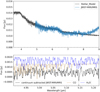 |
Fig. A.1 Stellar contribution to the JWST-MIRI/MRS spectrum. Top panel: JWST-MIRI/MRS spectrum of Sz28 and the modelled stellar spectrum, which has an offset of 0.009 Jy. Bottom panel: CO and H2O absorption slabs and the continuum-subtracted JWST-MIRI/MRS spectrum, highlighting their respective presence. |
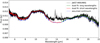 |
Fig. A.2 Interpolated dust continuum assumed (blue) together with the JWST-MIRI/MRS spectrum of Sz28 (black). The blue dots mark the locations used for interpolation. The continua provided by the dust fits for the short and long wavelength part of the spectrum are shown in red and green, respectively. |
Appendix B χ2 for molecules not quantitatively analysed
For several molecules where we attempted 0D slab model fits, we find that the remaining degeneracies in the column density and temperature are too large to warrant a quantitative analysis. We present in this appendix the χ2 maps of these species. They are labelled as ‘detected’ in Table 3. We do not provide such maps for CH3 and CH4 because we did not fit these molecules due to limitations defined in Sect. 3.2. We provide the χ2 map for C6H6 to illustrate the large error bars on the molecule that is relatively well constrained.
We used ![Mathematical equation: $\[\chi_{min }^2+2.3, ~\chi_{min }^2+6.2 \text { and } \chi_{min }^2+11.8\]$](/articles/aa/full_html/2024/09/aa50078-24/aa50078-24-eq30.png) as 1σ, 2σ, and 3σ confidence intervals (Avni 1976, Table 1 and Equation 6). The black contours represent the emitting radii of 0.01, 0.05, 0.1, 0.5, 1, 5 au. Table B.1 provides the parameters of the slabs shown in Fig. 2 for the detected molecules that are not well constrained and hence not analysed quantitatively. It also provides the total number of molecules
as 1σ, 2σ, and 3σ confidence intervals (Avni 1976, Table 1 and Equation 6). The black contours represent the emitting radii of 0.01, 0.05, 0.1, 0.5, 1, 5 au. Table B.1 provides the parameters of the slabs shown in Fig. 2 for the detected molecules that are not well constrained and hence not analysed quantitatively. It also provides the total number of molecules ![Mathematical equation: $\[\mathcal{N}\]$](/articles/aa/full_html/2024/09/aa50078-24/aa50078-24-eq31.png) for species that are optically thin.
for species that are optically thin.
Parameters of the 0D slab models used to show the ‘detected’ molecules in the JWST-MIRI/MRS spectrum of Sz28 along with number of molecules ![Mathematical equation: $\[\mathcal{N}\]$](/articles/aa/full_html/2024/09/aa50078-24/aa50078-24-eq32.png) .
.
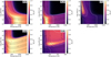 |
Fig. B.1 χ2 maps depicting the degeneracy in T and N. The white contours represent |
![Mathematical equation: $\[\chi_{min }^2+2.3, ~\chi_{min }^2+6.2 \text { and } \chi_{min }^2+11.8\]$](/articles/aa/full_html/2024/09/aa50078-24/aa50078-24-eq34.png)
Appendix C Detailed analysis of CO2
The JWST-MIRI/MRS spectrum of CO2, 13CO2 and the hot band of CO2 are shown in three different panels in Fig C.1. The temperatures for CO2 can vary from 100 to 250 K. The narrow width of the peak of CO2 drives the temperature solution towards 100 K. The location of the Q branch and the height of the hot band determines the column density N (Grant et al. 2023) and leads to values greater than 10185 cm−2; the emitting area is a scaling factor to best match the flux levels.
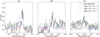 |
Fig. C.1 CO2 emission with slab models at different T at a constant N, where Rem is used as a scaling factor to match the flux levels. An Rem of 0.823 au is used for the model in red, and 0.069 au and 0.028 au for blue and green, respectively. Panel (a): Fundamental CO2 band. Panel (b): Fundamental 13CO2 band. Panel(c): Excited bending modes of CO2 and 13CO2. The 100 K (red) slab matches the JWST-MIRI/MRS data well. |
Appendix D Chemistry with canonical and enhanced C/O ratios
Table D.1 depicts the parameters used in the thermo-chemical disk models described in Sect. 5. The stellar luminosity is rescaled on the basis of the new distance reported in Galli et al. (2021). Figure D.1 shows the gas and dust temperature structure and the UV radiation field for both models. These are same in both the models. The canonical model has C/O = 0.45 whereas the enhanced model has a C/O = 2. Figure 4 shows the contours with a value of 10% of the maximum abundance of species in the canonical and enhanced C/O models. These maximum values of the abundance of species along with the maximum total column density and total column density at a radius of 0.1 au in both the models are listed in Table D.2. The maximum total column density is calculated by integrating all the molecules of a certain species from the surface to the midplane at every radii and the maximum of those are reported. Similarly, the total column density at 0.1 au is calculated by integrating all the molecules of a certain species at the radius of 0.1 au.
Figure D.2 shows the vertical H/H2 and the C+/C/CO transitions at a distance of 0.25 au. The H/H2 transition occurs deeper in the disk and the vertical range over which C remains abundant is extended in the enhanced C/O model. The H/H2 transition is mainly driven by the H2 formation on grains and photodissociation of H2 in the canonical model with C/O ratio of 0.45. The presence of unblocked carbon, H and H2 results in the formation of hydrocarbons in the disk atmosphere (Kanwar et al. 2024). H2 can then be destroyed through the abstraction of H either by hydrocarbons or C itself in the enhanced C/O model. Thus, the H/H2 transition is pushed deeper into the disk to the point where all the left-over carbon is locked in CO.
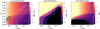 |
Fig. D.1 Dust temperature, gas temperature, and UV radiation field calculated from radiative transfer for the canonical and enhanced C/O models. The green and black contours show the dust continuum at 10 and 13.7 μm in first panel. The white contours in the second panel show the gas temperature corresponding to 140 K and 475 K. The black contour shows the Aυ=1 mag in the last panel. The dotted white contours represent the values corresponding to the tick marks of the color scale. |
In the following, we explain the analysis of the formation/destruction pathways for C2H2 and C6H6 in more detail. We study these in the models described in Sect. 5.1. The models with C/O ratios of 0.45 and 2 are referred to as canonical and enhanced models, respectively. We analysed these pathways at a grid point that lies in the surface emitting layer of C2H2. The characteristics describing the grid point are Tgas = 270 K and ![Mathematical equation: $\[T_{\text {dust }}=230 \mathrm{~K}, n_{\langle\mathrm{H}\rangle}=6.4 \cdot 10^{10} \mathrm{~cm}^{-3}, A_{\mathrm{V}}^{{ver }}=0.018, A_{\mathrm{V}}^{{rad }}=1.1\]$](/articles/aa/full_html/2024/09/aa50078-24/aa50078-24-eq35.png) .
.
The following set of reactions were dominant formation pathways for C2H2 in the model with the canonical C/O similar to the findings of Kanwar et al. (2024):
![Mathematical equation: $\[\mathrm{C}_2 \mathrm{H}_3{ }^{+}+\mathrm{e}^{-} \rightarrow \mathrm{C}_2 \mathrm{H}_2+\mathrm{H}\]$](/articles/aa/full_html/2024/09/aa50078-24/aa50078-24-eq36.png) (D.1)
(D.1)
![Mathematical equation: $\[\mathrm{O}+\mathrm{H}_2 \mathrm{CCC} \rightarrow \mathrm{CO}+\mathrm{C}_2 \mathrm{H}_2\]$](/articles/aa/full_html/2024/09/aa50078-24/aa50078-24-eq37.png) (D.2)
(D.2)
![Mathematical equation: $\[\mathrm{O}+\mathrm{C}_3 \mathrm{H}_3{ }^{+} \rightarrow \mathrm{HCO}^{+}+\mathrm{C}_2 \mathrm{H}_2\]$](/articles/aa/full_html/2024/09/aa50078-24/aa50078-24-eq38.png) (D.3)
(D.3)
![Mathematical equation: $\[\mathrm{C}_3 \mathrm{H}_3^{~+}+\mathrm{e}^{-} \rightarrow \mathrm{CH}+\mathrm{C}_2 \mathrm{H}_2\]$](/articles/aa/full_html/2024/09/aa50078-24/aa50078-24-eq39.png) (D.4)
(D.4)
As is evident from reactions D.2 and D.3, the chemistry is driven by O. The contribution of reaction D.2 in forming C2H2 decreased from ~2% in the canonical model to ~0.01% in the enhanced C/O ratio model. This is a result of depleting O to enhance the C/O ratio. The following reactions then become more important than reactions D.2 and D.3:
![Mathematical equation: $\[\mathrm{C}+\mathrm{C}_2 \mathrm{H}_2^{~+} \rightarrow \mathrm{C}_2 \mathrm{H}_2+\mathrm{C}^{+}\]$](/articles/aa/full_html/2024/09/aa50078-24/aa50078-24-eq40.png) (D.5)
(D.5)
![Mathematical equation: $\[\mathrm{C}_2 \mathrm{H}+\mathrm{H}+\mathrm{M} \rightarrow \mathrm{C}_2 \mathrm{H}_2+\mathrm{M}\]$](/articles/aa/full_html/2024/09/aa50078-24/aa50078-24-eq41.png) (D.6)
(D.6)
These reactions were active in the canonical model but their rates increased as the elemental abundance of O is depleted in the enhanced C/O model. Hence, the dominant reaction pathways only shuffle in their relative importance when depleting O.
The destruction reactions for benzene in both models at the same grid point (see above) are:
![Mathematical equation: $\[\mathrm{C}_6 \mathrm{H}_6+h v \rightarrow \mathrm{C}_2 \mathrm{H}_2+\mathrm{CH}_2 \mathrm{CHCCH}\]$](/articles/aa/full_html/2024/09/aa50078-24/aa50078-24-eq42.png) (D.7)
(D.7)
![Mathematical equation: $\[\mathrm{C}^{+}+\mathrm{C}_6 \mathrm{H}_6 \rightarrow \mathrm{C}_6 \mathrm{H}_6^{~+}+\mathrm{C}\]$](/articles/aa/full_html/2024/09/aa50078-24/aa50078-24-eq43.png) (D.8)
(D.8)
![Mathematical equation: $\[\mathrm{C}^{+}+\mathrm{C}_6 \mathrm{H}_6 \rightarrow \mathrm{C}_5 \mathrm{H}_3^{~+}+\mathrm{C}_2 \mathrm{H}_3\]$](/articles/aa/full_html/2024/09/aa50078-24/aa50078-24-eq44.png) (D.9)
(D.9)
![Mathematical equation: $\[\mathrm{C}^{+}+\mathrm{C}_6 \mathrm{H}_6 \rightarrow \mathrm{C}_7 \mathrm{H}_5^{~+}+\mathrm{H}\]$](/articles/aa/full_html/2024/09/aa50078-24/aa50078-24-eq45.png) (D.10)
(D.10)
Reaction D.7 contributes −85% to the destruction of C6H6 in the canonical C/O model, which becomes ~23% in the enhanced C/O model. Reaction D.8 is the next most dominant reaction contributing ~10% in the canonical C/O model, which becomes ~52% in the model with enhanced C/O. This redistribution in the contribution is due to the increased abundance of C2H2 which promotes reaction D.5, thus increasing C+. The other way to form C+ is via UV photo-ionisation of C. The C2H2 abundance increase is due to the depletion of O and thus enhancement of the C/O ratio.
Parameters for the thermo-chemical disk model used in Sect. 5 adopted from Greenwood et al. (2017).
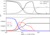 |
Fig. D.2 Effect of change in C/O ratio on various transitions. Top panel: H/H2 transition in the canonical (dashed lines) and enhanced C/O (solid lines) model at the radius of 0.25 au. Bottom panel: C+/C/CO transition layers in both models at the same radius. |
Figures D.3, D.4, D.5 and D.6 show the 2D abundances of various species obtained from the thermo-chemical disk models. The abundances of the hydrocarbons increase in the surface layers when we change C/O from 0.45 (canonical) to 2.0 (enhanced). The blank regions in the abundance plot of CO for the enhanced model are due to the failure in solving the chemical reaction rate network at those locations. This might be because we did not model a fully self-consistent solution (the gas temperature structure is taken from the canonical model).
Maximum total column density (Nmax), radius at which Nmax is reached, maximum abundance of species (ϵmax), and the total column density at a radius of 0.1 au (N) in models with canonical and enhanced C/O elemental ratios.
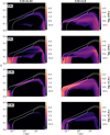 |
Fig. D.3 Abundances of various hydrocarbons in the canonical (0.45, left column) and enhanced (2.0, right column) C/O ratio models. The white contours correspond to gas temperatures of 140 K and 475 K. |
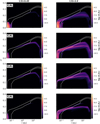 |
Fig. D.4 Abundances of various hydrocarbons in the canonical (0.45, left column) and enhanced (2.0, right column) C/O ratio models. The white contours correspond to gas temperatures of 140 K and 475 K. |
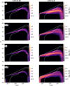 |
Fig. D.5 Abundances of various hydrocarbons in the canonical (0.45, left column) and enhanced (2.0, right column) C/O ratio models. The white contours correspond to gas temperature of 140 K and 475 K. |
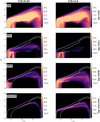 |
Fig. D.6 Abundances of various species in the canonical (0.45, left column) and enhanced (2.0, right column) C/O ratio models. The white contours correspond to gas temperature of 140 K and 475 K. |
References
- Agúndez, M., Cernicharo, J., & Goicoechea, J. R. 2008, A&A, 483, 831 [NASA ADS] [CrossRef] [EDP Sciences] [Google Scholar]
- Anders, E., & Grevesse, N. 1989, Geochim. Cosmochim. Acta, 53, 197 [Google Scholar]
- Apai, D., Pascucci, I., Bouwman, J., et al. 2005, Science, 310, 834 [NASA ADS] [CrossRef] [Google Scholar]
- Arabhavi, A. M., Kamp, I., Henning, T., et al. 2024, Science, 384, 1086 [NASA ADS] [CrossRef] [Google Scholar]
- Argyriou, I., Glasse, A., Law, D. R., et al. 2023, A&A, 675, A111 [NASA ADS] [CrossRef] [EDP Sciences] [Google Scholar]
- Avni, Y. 1976, ApJ, 210, 642 [NASA ADS] [CrossRef] [Google Scholar]
- Barrado y Navascués, D., & Martín, E. L. 2003, AJ, 126, 2997 [Google Scholar]
- Barrado y Navascués, D., Stauffer, J. R., Morales-Calderón, M., et al. 2007, ApJ, 664, 481 [CrossRef] [Google Scholar]
- Bast, J. E., Lahuis, F., van Dishoeck, E. F., & Tielens, A. G. G. M. 2013, A&A, 551, A118 [NASA ADS] [CrossRef] [EDP Sciences] [Google Scholar]
- Bergin, E. A., Du, F., Cleeves, L. I., et al. 2016, ApJ, 831, 101 [Google Scholar]
- Brott, I., & Hauschildt, P. H. 2005, in The Three-Dimensional Universe with Gaia, eds. C. Turon, K. S. O’Flaherty, & M. A. C. Perryman, ESA Special Publication, 576, 565 [NASA ADS] [Google Scholar]
- Bushouse, H., Eisenhamer, J., Dencheva, N., et al. 2023, JWST Calibration Pipeline, Zenodo [Google Scholar]
- Carnall, A. C. 2017, arXiv e-prints [arXiv:1705.05165] [Google Scholar]
- Carr, J. S., & Najita, J. R. 2011, ApJ, 733, 102 [NASA ADS] [CrossRef] [Google Scholar]
- Christiaens, V., Gonzalez, C., Farkas, R., et al. 2023, J. Open Source Softw., 8, 4774 [NASA ADS] [CrossRef] [Google Scholar]
- Christiaens, V., Samland, M., Gasman, D., Temmink, M., & Perotti, G. 2024, MINDS: Hybrid pipeline for the reduction of JWST/MIRI-MRS data, Astrophysics Source Code Library, [record ascl:2403.007] [Google Scholar]
- Delahaye, T., Armante, R., Scott, N. A., et al. 2021, J. Mol. Spectrosc., 380, 111510 [NASA ADS] [CrossRef] [Google Scholar]
- Dorschner, J., Begemann, B., Henning, T., Jaeger, C., & Mutschke, H. 1995, A&A, 300, 503 [Google Scholar]
- Dressing, C. D., & Charbonneau, D. 2015, ApJ, 807, 45 [Google Scholar]
- Dubrulle, B., Morfill, G., & Sterzik, M. 1995, Icarus, 114, 237 [Google Scholar]
- Dyer, S., & Dyer, J. 2001, IEEE Instrum. Meas. Mag., 4, 44 [CrossRef] [Google Scholar]
- Fabian, D., Jäger, C., Henning, T., Dorschner, J., & Mutschke, H. 2000, A&A, 364, 282 [Google Scholar]
- Franceschi, R., Henning, T., Tabone, B., et al. 2024, A&A, 687, A96 [NASA ADS] [CrossRef] [EDP Sciences] [Google Scholar]
- Galli, P. A. B., Bouy, H., Olivares, J., et al. 2021, A&A, 646, A46 [NASA ADS] [CrossRef] [EDP Sciences] [Google Scholar]
- Gomez Gonzalez, C. A., Wertz, O., Absil, O., et al. 2017, AJ, 154, 7 [Google Scholar]
- Gondoin, P. 2006, A&A, 454, 595 [NASA ADS] [CrossRef] [EDP Sciences] [Google Scholar]
- Gordon, I. E., Rothman, L. S., Hargreaves, R. J., et al. 2022, J. Quant. Spec. Radiat. Transf., 277, 107949 [NASA ADS] [CrossRef] [Google Scholar]
- Grant, S. L., van Dishoeck, E. F., Tabone, B., et al. 2023, ApJ, 947, L6 [NASA ADS] [CrossRef] [Google Scholar]
- Greenwood, A. J., Kamp, I., Waters, L. B. F. M., et al. 2017, A&A, 601, A44 [NASA ADS] [CrossRef] [EDP Sciences] [Google Scholar]
- Güdel, M., Briggs, K. R., Arzner, K., et al. 2007, A&A, 468, 353 [Google Scholar]
- Güdel, M., Lahuis, F., Briggs, K. R., et al. 2010, A&A, 519, A113 [CrossRef] [EDP Sciences] [Google Scholar]
- Hakim, K., Spaargaren, R., Grewal, D. S., et al. 2019, Astrobiology, 19, 867 [NASA ADS] [CrossRef] [Google Scholar]
- Helmich, F. P. 1996, PhD thesis, University of Leiden, Netherlands [Google Scholar]
- Henning, T. 2010, ARA&A, 48, 21 [Google Scholar]
- Henning, T., & Stognienko, R. 1996, A&A, 311, 291 [NASA ADS] [Google Scholar]
- Henning, T., & Semenov, D. 2013, Chem. Rev., 113, 9016 [Google Scholar]
- Henning, T., Kamp, I., Samland, M., et al. 2024, PASP, 136, 054302 [NASA ADS] [CrossRef] [Google Scholar]
- Jaeger, C., Molster, F. J., Dorschner, J., et al. 1998, A&A, 339, 904 [Google Scholar]
- Jang, H., Waters, L. B. F. M., Kamp, I., & Dullemond, C. P. 2024, A&A, 687, A275 [NASA ADS] [CrossRef] [EDP Sciences] [Google Scholar]
- Juhász, A., Bouwman, J., Henning, T., et al. 2010, ApJ, 721, 431 [Google Scholar]
- Kaeufer, T., Min, M., Woitke, P., Kamp, I., & Arabhavi, A. M. 2024, A&A, 687, A209 [NASA ADS] [CrossRef] [EDP Sciences] [Google Scholar]
- Kamp, I., Thi, W. F., Woitke, P., et al. 2017, A&A, 607, A41 [NASA ADS] [CrossRef] [EDP Sciences] [Google Scholar]
- Kamp, I., Henning, T., Arabhavi, A. M., et al. 2023, Faraday Discuss., 245, 112 [NASA ADS] [CrossRef] [Google Scholar]
- Kanwar, J., Kamp, I., Woitke, P., et al. 2024, A&A, 681, A22 [NASA ADS] [CrossRef] [EDP Sciences] [Google Scholar]
- Kessler-Silacci, J. E., Dullemond, C. P., Augereau, J. C., et al. 2007, ApJ, 659, 680 [NASA ADS] [CrossRef] [Google Scholar]
- Krijt, S., Kama, M., McClure, M., et al. 2022, arXiv e-prints [arXiv:2203.10056] [Google Scholar]
- Kurtovic, N. T., Pinilla, P., Long, F., et al. 2021, A&A, 645, A139 [EDP Sciences] [Google Scholar]
- Lepeshkin, S., Baturin, V., Naumova, A., & Oganov, A. 2022, J. Phys. Chem. Lett., 13, 7600 [Google Scholar]
- Lichtenberg, T., Bower, D. J., Hammond, M., et al. 2021, J. Geophys. Res. (Planets), 126, e06711 [NASA ADS] [Google Scholar]
- Liebert, J., & Probst, R. G. 1987, ARA&A, 25, 473 [Google Scholar]
- Liu, B., Lambrechts, M., Johansen, A., Pascucci, I., & Henning, T. 2020, A&A, 638, A88 [EDP Sciences] [Google Scholar]
- Liu, Y., Pascucci, I., & Henning, T. 2019, A&A, 623, A106 [NASA ADS] [CrossRef] [EDP Sciences] [Google Scholar]
- Long, F., Herczeg, G. J., Pascucci, I., et al. 2017, ApJ, 844, 99 [Google Scholar]
- Luhman, K. L., & Mamajek, E. E. 2012, ApJ, 758, 31 [Google Scholar]
- Mah, J., Bitsch, B., Pascucci, I., & Henning, T. 2023, A&A, 677, A7 [Google Scholar]
- Mah, J., Savvidou, S., & Bitsch, B. 2024, A&A, 686, L17 [NASA ADS] [CrossRef] [EDP Sciences] [Google Scholar]
- Manara, C. F., Testi, L., Herczeg, G. J., et al. 2017, A&A, 604, A127 [NASA ADS] [CrossRef] [EDP Sciences] [Google Scholar]
- Manara, C. F., Ansdell, M., Rosotti, G. P., et al. 2023, in Protostars and Planets VII, eds. S. Inutsuka, Y. Aikawa, T. Muto, K. Tomida, & M. Tamura, Astronomical Society of the Pacific Conference Series, 534, 539 [NASA ADS] [Google Scholar]
- McElroy, D., Walsh, C., Markwick, A. J., et al. 2013, A&A, 550, A36 [NASA ADS] [CrossRef] [EDP Sciences] [Google Scholar]
- McEwan, M. J., Scott, G. B. I., Adams, N. G., et al. 1999, ApJ, 513, 287 [Google Scholar]
- Min, M., Waters, L. B. F. M., de Koter, A., et al. 2007, A&A, 462, 667 [NASA ADS] [CrossRef] [EDP Sciences] [Google Scholar]
- Mollière, P., Molyarova, T., Bitsch, B., et al. 2022, ApJ, 934, 74 [CrossRef] [Google Scholar]
- Öberg, K. I., Murray-Clay, R., & Bergin, E. A. 2011, ApJ, 743, L16 [Google Scholar]
- Oliveira, I., Olofsson, J., Pontoppidan, K. M., et al. 2011, ApJ, 734, 51 [CrossRef] [Google Scholar]
- Olofsson, J., Augereau, J. C., van Dishoeck, E. F., et al. 2009, A&A, 507, 327 [NASA ADS] [CrossRef] [EDP Sciences] [Google Scholar]
- Pascucci, I., Apai, D., Luhman, K., et al. 2009, ApJ, 696, 143 [Google Scholar]
- Pascucci, I., Herczeg, G., Carr, J. S., & Bruderer, S. 2013, ApJ, 779, 178 [NASA ADS] [CrossRef] [Google Scholar]
- Pascucci, I., Testi, L., Herczeg, G. J., et al. 2016, ApJ, 831, 125 [Google Scholar]
- Perotti, G., Christiaens, V., Henning, T., et al. 2023, Nature, 620, 516 [NASA ADS] [CrossRef] [Google Scholar]
- Pinilla, P. 2022, Eur. Phys. J. Plus, 137, 1206 [NASA ADS] [CrossRef] [Google Scholar]
- Pontoppidan, K. M., Salyk, C., Blake, G. A., et al. 2010, ApJ, 720, 887 [CrossRef] [Google Scholar]
- Qi, C., Öberg, K. I., Wilner, D. J., et al. 2013, Science, 341, 630 [Google Scholar]
- Ratzenböck, S., Großschedl, J. E., Alves, J., et al. 2023, A&A, 678, A71 [NASA ADS] [CrossRef] [EDP Sciences] [Google Scholar]
- Rieke, G. H., Wright, G., Böker, T., et al. 2015, PASP, 127, 584 [NASA ADS] [CrossRef] [Google Scholar]
- Rigby, J., Perrin, M., McElwain, M., et al. 2023, PASP, 135, 048001 [NASA ADS] [CrossRef] [Google Scholar]
- Sabotta, S., Schlecker, M., Chaturvedi, P., et al. 2021, A&A, 653, A114 [NASA ADS] [CrossRef] [EDP Sciences] [Google Scholar]
- Salyk, C., Pontoppidan, K. M., Blake, G. A., et al. 2008, ApJ, 676, L49 [NASA ADS] [CrossRef] [Google Scholar]
- Schlecker, M., Burn, R., Sabotta, S., et al. 2022, A&A, 664, A180 [NASA ADS] [CrossRef] [EDP Sciences] [Google Scholar]
- Servoin, J. L., & Piriou, B. 1973, Physica Status Solidi B Basic Res., 55, 677 [NASA ADS] [CrossRef] [Google Scholar]
- Spitzer, W. G., & Kleinman, D. A. 1960, Phys. Rev., 121, 1324 [Google Scholar]
- Tabone, B., Bettoni, G., van Dishoeck, E. F., et al. 2023, Nat. Astron., 7, 805 [NASA ADS] [CrossRef] [Google Scholar]
- Temmink, M., van Dishoeck, E. F., Grant, S. L., et al. 2024, A&A, 686, A117 [NASA ADS] [CrossRef] [EDP Sciences] [Google Scholar]
- Thiabaud, A., Marboeuf, U., Alibert, Y., Leya, I., & Mezger, K. 2015, A&A, 580, A30 [NASA ADS] [CrossRef] [EDP Sciences] [Google Scholar]
- Walsh, C., Nomura, H., & van Dishoeck, E. 2015, A&A, 582, A88 [NASA ADS] [CrossRef] [EDP Sciences] [Google Scholar]
- Wells, M., Pel, J. W., Glasse, A., et al. 2015, PASP, 127, 646 [NASA ADS] [CrossRef] [Google Scholar]
- Woitke, P., Kamp, I., & Thi, W. F. 2009, A&A, 501, 383 [NASA ADS] [CrossRef] [EDP Sciences] [Google Scholar]
- Woitke, P., Min, M., Pinte, C., et al. 2016, A&A, 586, A103 [NASA ADS] [CrossRef] [EDP Sciences] [Google Scholar]
- Woitke, P., Min, M., Thi, W. F., et al. 2018, A&A, 618, A57 [NASA ADS] [CrossRef] [EDP Sciences] [Google Scholar]
- Woitke, P., Thi, W. F., Arabhavi, A. M., et al. 2024, A&A, 683, A219 [NASA ADS] [CrossRef] [EDP Sciences] [Google Scholar]
- Woods, P. M., & Willacy, K. 2007, ApJ, 655, L49 [NASA ADS] [CrossRef] [Google Scholar]
- Woods, P. M., & Willacy, K. 2009, ApJ, 693, 1360 [Google Scholar]
- Wright, G. S., Wright, D., Goodson, G. B., et al. 2015, PASP, 127, 595 [NASA ADS] [CrossRef] [Google Scholar]
- Wright, G. S., Rieke, G. H., Glasse, A., et al. 2023, PASP, 135, 048003 [NASA ADS] [CrossRef] [Google Scholar]
- Xie, C., Pascucci, I., Long, F., et al. 2023, ApJ, 959, L25 [NASA ADS] [CrossRef] [Google Scholar]
‘Magic’ refers to the more energetically stable species as reported in Lepeshkin et al. (2022).
All Tables
S/Ns provided by ETC along with the median continuum flux in each band where molecules are detected.
Parameters of the 0D slab models used to show the ‘detected’ molecules in the JWST-MIRI/MRS spectrum of Sz28 along with number of molecules .
Parameters for the thermo-chemical disk model used in Sect. 5 adopted from Greenwood et al. (2017).
Maximum total column density (Nmax), radius at which Nmax is reached, maximum abundance of species (ϵmax), and the total column density at a radius of 0.1 au (N) in models with canonical and enhanced C/O elemental ratios.
All Figures
|
Fig. 1 JWST-MIRI/MRS spectrum of Sz28. The detected molecular species and the dust features are labelled. The spectrum from Spitzer is depicted in grey. The red question mark (?) indicates the unidentified spectral features and the red horizontal lines show their wavelength range. The Q branches of the molecules are shown as solid lines along with their identified isotopologues, if any, as dotted lines. |
| In the text | |
|
Fig. 2 Top panel: continuum-subtracted JWST-MIRI/MRS spectrum of Sz28 showing the total model (addition of slabs of all the detected molecules) in the wavelength region 12–17 μm. Bottom two panels: individual contribution of the slab models for the detected molecular species. The slab model fits are performed over the wavelength window shown at the bottom of the panel as a straight line for a molecule in their corresponding colour. The slab parameters of the spectrum of not well-constrained molecules can be found in Table B.1. |
| In the text | |
|
Fig. 3 Slab model for CH4 shown in red along with the zoomed-in JWST-MIRI/MRS spectrum of Sz28. The parameters from the 0D slab models for the represented slab can be found in Table B.1. |
| In the text | |
|
Fig. 4 Abundance contours corresponding to 10% of the maximum abundance of the hydrocarbons detected in disks around VLMSs in the canonical and enhanced model with C/O of 0.45 and 2.0, respectively. The white contours correspond to the gas temperatures of 140 K and 475 K. The Aυ =1 mag contour is shown in black. |
| In the text | |
|
Fig. A.1 Stellar contribution to the JWST-MIRI/MRS spectrum. Top panel: JWST-MIRI/MRS spectrum of Sz28 and the modelled stellar spectrum, which has an offset of 0.009 Jy. Bottom panel: CO and H2O absorption slabs and the continuum-subtracted JWST-MIRI/MRS spectrum, highlighting their respective presence. |
| In the text | |
|
Fig. A.2 Interpolated dust continuum assumed (blue) together with the JWST-MIRI/MRS spectrum of Sz28 (black). The blue dots mark the locations used for interpolation. The continua provided by the dust fits for the short and long wavelength part of the spectrum are shown in red and green, respectively. |
| In the text | |
|
Fig. B.1 χ2 maps depicting the degeneracy in T and N. The white contours represent |
| In the text | |
|
Fig. C.1 CO2 emission with slab models at different T at a constant N, where Rem is used as a scaling factor to match the flux levels. An Rem of 0.823 au is used for the model in red, and 0.069 au and 0.028 au for blue and green, respectively. Panel (a): Fundamental CO2 band. Panel (b): Fundamental 13CO2 band. Panel(c): Excited bending modes of CO2 and 13CO2. The 100 K (red) slab matches the JWST-MIRI/MRS data well. |
| In the text | |
|
Fig. D.1 Dust temperature, gas temperature, and UV radiation field calculated from radiative transfer for the canonical and enhanced C/O models. The green and black contours show the dust continuum at 10 and 13.7 μm in first panel. The white contours in the second panel show the gas temperature corresponding to 140 K and 475 K. The black contour shows the Aυ=1 mag in the last panel. The dotted white contours represent the values corresponding to the tick marks of the color scale. |
| In the text | |
|
Fig. D.2 Effect of change in C/O ratio on various transitions. Top panel: H/H2 transition in the canonical (dashed lines) and enhanced C/O (solid lines) model at the radius of 0.25 au. Bottom panel: C+/C/CO transition layers in both models at the same radius. |
| In the text | |
|
Fig. D.3 Abundances of various hydrocarbons in the canonical (0.45, left column) and enhanced (2.0, right column) C/O ratio models. The white contours correspond to gas temperatures of 140 K and 475 K. |
| In the text | |
|
Fig. D.4 Abundances of various hydrocarbons in the canonical (0.45, left column) and enhanced (2.0, right column) C/O ratio models. The white contours correspond to gas temperatures of 140 K and 475 K. |
| In the text | |
|
Fig. D.5 Abundances of various hydrocarbons in the canonical (0.45, left column) and enhanced (2.0, right column) C/O ratio models. The white contours correspond to gas temperature of 140 K and 475 K. |
| In the text | |
|
Fig. D.6 Abundances of various species in the canonical (0.45, left column) and enhanced (2.0, right column) C/O ratio models. The white contours correspond to gas temperature of 140 K and 475 K. |
| In the text | |
Current usage metrics show cumulative count of Article Views (full-text article views including HTML views, PDF and ePub downloads, according to the available data) and Abstracts Views on Vision4Press platform.
Data correspond to usage on the plateform after 2015. The current usage metrics is available 48-96 hours after online publication and is updated daily on week days.
Initial download of the metrics may take a while.