| Issue |
A&A
Volume 699, July 2025
|
|
|---|---|---|
| Article Number | A142 | |
| Number of page(s) | 21 | |
| Section | Galactic structure, stellar clusters and populations | |
| DOI | https://doi.org/10.1051/0004-6361/202452195 | |
| Published online | 08 July 2025 | |
Beyond the main sequence: Binary evolution pathways to blue stragglers in the Gaia era
I. Galactic open and globular clusters
Institute of Astrophysics, Pontificia Universidad Católica de Chile,
Avenida Vicuńa Mackenna 4860,
7820436
Macul,
Santiago,
Chile
★ Corresponding authors: This email address is being protected from spambots. You need JavaScript enabled to view it.
; This email address is being protected from spambots. You need JavaScript enabled to view it.
; This email address is being protected from spambots. You need JavaScript enabled to view it.
Received:
10
September
2024
Accepted:
26
March
2025
Abstract
Context. The study of blue straggler stars (BSSs) provides insight into the mechanisms of stellar mass exchange during binary stellar evolution and the complex gravitational interactions within dense stellar systems. In combination, they enhance our understanding of the possible life cycles of stars and the evolutionary pathways of star clusters.
Aims. We study the populations of BSSs in 41 globular clusters (GCs) and 42 open clusters (OCs) based on photometry, proper motion, and parallax from the Gaia Data Release 3 (DR3). We confirm their cluster membership. We find a total of 4399 BSSs: All GCs show BSSs (3965 or ∼ 90% of the sample), whereas only 42 out of 129 studied OCs show BSSs (434 or ∼ 10% of the sample). Clusters younger than ∼ 500 Myr do not host any BSSs.
Methods. We derived their astrophysical parameters such as effective temperature, surface gravity, and mass based on colortemperature relations, isochrone models, and Gaia DR3 spectroscopy (if available). We found values for Teff=(6800 ± 585) K and (7570 ± 1400) K and an average mass of ⟨MBSS⟩=(1.02 ± 0.1) M⊙ and ⟨ MBSS⟩=(1.75 ± 0.45) M⊙ for GCs and OCs, respectively. We finally computed the difference of the BSS mass and the main-sequence turn-off (MSTO) mass of its respective cluster, normalized by the MSTO mass, for every identified BSS.
Results. Based on this parameter and on the BSSs ages derived from isochrone models, we find that (i) GC BSSs that are most likely to be formed through collisions show a boost for ages ∼ 1 – 2 Gyr. This agrees with the ages for core-collapse events in GCs that were reported in previous studies. We also find (ii) a double sequence for GC BSSs that might indicate a pre- or post-merger or close-binary scenario.
Key words: blue stragglers / stars: fundamental parameters / globular clusters: general / open clusters and associations: general
CATA Research Fellow.
© The Authors 2025
 Open Access article, published by EDP Sciences, under the terms of the Creative Commons Attribution License (https://creativecommons.org/licenses/by/4.0), which permits unrestricted use, distribution, and reproduction in any medium, provided the original work is properly cited.
This article is published in open access under the Subscribe to Open model. This email address is being protected from spambots. You need JavaScript enabled to view it. to support open access publication.
1 Introduction
Blue straggler stars (BSSs) are stars that appear to be younger and more massive than the bulk of other stars in their host stellar population. They are characterized by their location in the color-magnitude diagram (CMD), where they appear hotter and bluer than their main-sequence (MS) neighbors.
Blue straggler stars were first identified by Sandage (1953) through his observations of the globular cluster (GC) Messier 3 (M3), and some years later, they were reported in the open cluster (OC) NGC 7786 by Burbidge & Sandage (1958). Ever since, their presence has been noted in distinct structures: as field stars (Preston & Sneden 2000; Jofré et al. 2016), in OB associations (Mathys 1987), in the Galactic bulge (Clarkson et al. 2011), and in dwarf galaxies (Da Costa 1984; Mapelli et al. 2009).
Blue straggler stars challenge the standard theory of stellar evolution, which states that the more massive a star, the faster it evolves. For this reason, these stars should have evolved off the MS branch a long time ago, but they still populate this branch as an apparent extension of the MS in a CMD. Three scenarios have been proposed to explain their formation: (i) Mass transfer (MT) in binary systems (McCrea 1964), where a star receives material from its companion. This extends its life. (ii) Stars formed through collisions or mergers (Hills & Day 1976; Lombardi et al. 2002). (iii) In hierarchical triple systems, magnetized winds or stellar evolution cause the loss of angular momentum in a multiple system, which leads to collisions (or MT) between the stars that conform the system (Perets & Fabrycky 2009; Naoz & Fabrycky 2014). It has been shown that the BSS properties scale with different astrophysical parameters of their parent cluster (Knigge et al. 2009; Leigh et al. 2011; Jadhav & Subramaniam 2021), which might help us in principle to constrain which of the formation pathways dominates. It is important to mention, however, that these formation mechanisms most likely coexist, that is, they operate simultaneously (Mapelli et al. 2006; Leigh et al. 2011).
Ferraro et al. (2009) found a double sequence of BSSs in the GC M30: a blue and a red BSS sequence, which were both roughly aligned with the zero-age MS (ZAMS). The authors argued that the distinction between these two BSS sequences may be due to their origin: collisional BSSs (Col-BSSs), which are deemed more massive and hotter and therefore appear bluer in the CMD, whereas MT-BSSs would be less massive, mildly cooler than Col-BSSs, and would therefore appear as a redder BSS sequence. This is not an isolated case. Double/multiple sequences of BSSs have been reported for more GCs, such as NGC 362 (Dalessandro et al. 2013), NGC 1261 (Simunovic et al. 2014), M15 (Beccari et al. 2019), and NGC 6256 (Cadelano et al. 2022). The explanation given for all these cases leads to a core-collapse scenario of the host GC in which the central interactions between stars increase, resulting in the formation of BSSs. Therefore, a double/multiple BSS sequence could be a vestige of this event. It also has been found that some BSSs show a hot companion (Gosnell et al. 2015; Sindhu et al. 2019), which provides supporting evidence for the MT formation scenario in action. Linking these concepts, Dattatrey et al. (2023, hereafter D23) have analyzed the spectral energy distribution (SED) for multiple BSSs in the GC NGC 362. They demonstrated that BSSs with and without a hot companion lie on the red and blue BSS sequence, respectively, which agrees with the explanations provided by Dalessandro et al. (2013) for the same GC. More recently, a double BSS sequence has also been detected in the OC Berkeley 17 by Rao et al. (2023a). Given the lack of core collapse in OCs and the accordingly considerable attenuation of the Col-BSS formation channel, the authors argued that this double BSS sequence might be due to a significant difference in BSS rotational velocities, the presence of multiple stellar populations (MSP), or to extinction effects (for more details see Rao et al. 2023a, and references therein).
The arrival of the Gaia mission (Gaia Collaboration 2016) with data for almost 1.7 billion objects has opened new opportunities to explore the kinematics of our Galaxy and has helped us to identify and confirm the cluster membership of stars in GCs (Vasiliev & Baumgardt 2021) and OCs (Cantat-Gaudin et al. 2018; Dias et al. 2021). Gaia faces limitations in overcrowded regions (large errors for its astrometric parameters because it cannot reliably resolve sources), however, such as GC centers. Nevertheless, BSS studies in crowded regions are covered by HST1 data, which can lead to high-accuracy measurements in the densest regions (e.g. Baldwin et al. 2016), and because HST features a broader SED coverage than Gaia, BSSs can also be easily identified through the so-called UV-route (Ferraro et al. 1997; Raso et al. 2017; Ferraro et al. 2018, and references therein).
It is particularly interesting to analyze the radial distribution of BSSs, especially in the inner regions of clusters. Since BSSs are more massive compared with other stars in the same cluster, they tend to undergo efficient mass segregation, that is, they sink to the inner parts of the cluster (Contreras Ramos et al. 2012). It is therefore expected that these peculiar stars can be used to measure the dynamical state of a cluster, that is, they can be used as dynamical clocks in GCs (Ferraro et al. 2012, 2023) and OCs (Rao et al. 2021, 2023b).
Gaia Data Release 3 (Gaia Collaboration 2023, hereafter DR3) for OCs does not suffer from overcrowding, even in the core of OCs. For example, using Gaia Data Release 2 (Gaia Collaboration 2018, hereafter DR2), Rain et al. (2021, hereafter R21) created a catalog for 408 BSSs in different OCs, while Jadhav & Subramaniam (2021, hereafter JS21) have studied the scaling relations of BSSs and their parent OCs. Gaia DR2 has also opened new opportunities for studying GCs and their kinematics (e.g., Vasiliev & Baumgardt 2021). Several HST-based studies have previously characterized BSSs in GCs (Simunovic & Puzia 2016). The limitation of HST-based studies was, however, that they can only cover the inner regions of clusters, that is, from the center up to about the half-light radius, rhl. For example, data from the HST UV Globular Cluster Survey (Piotto et al. 2015; Nardiello et al. 2018, also known as “HUGS”) cover this region and do not include the outskirts of the target GCs. Therefore, combining Gaia DR3 with HST will help us to analyze the radial distribution of BSSs in GCs from the core to the outer radii and to determine whether the GCs are dynamically settled. In the case of OCs, Gaia DR3 alone can be used to study their dynamical evolution. Hence, a homogeneous catalog of BSSs in GCs and OCs is necessary to understand their formation channels and to examine the dynamical evolution of their host clusters.
We use Gaia DR3 to create a new homogeneous BSSs catalog of GCs and OCs that differs from previous catalogs (Rain et al. 2021; Simunovic & Puzia 2016). This work includes BSSs that were previously not covered due to the radial coverage limitations of prior work. This study also provides various newly derived astrophysical parameters of BSSs from the color-temperature relation, isochrone models, and DR3 spectra.
This paper is organized as follows. In Section 2, we describe the selection of cluster members and the selection of BSSs. We introduce the different methods we applied to obtain different astrophysical parameters for the BSS cluster members we identified. In Section 3, we present our results for the total number of identified BSSs and their fraction with respect to their parent cluster MS stars, as well as the distributions for the derived astrophysical BSS parameters. We analyze the results and compare them with previous results in the literature, and we discuss the implications. We finally discuss possible uses and extensions for the identified BSS sample. In Section 4, we summarize the main results of this work.
2 Data selection
To select the clusters studied in this work, we first select GCs and OCs that have a significant number of members based on previous studies. We select all GCs from the catalog by Vasiliev & Baumgardt (2021) with at least 1000 identified member stars and all OCs from the catalog by Dias et al. (2021) with at least 350 identified member stars. We find 41 GCs and 129 OCs following the above criteria.
2.1 Star cluster membership
To identify cluster members, we apply a technique developed and used by Cordoni et al. (2018, hereafter C18), with a minor change for OCs (see step 2), which has also been used by Cordoni et al. (2020) for GCs. Our procedure is summarized as follows:
First, we select data from Gaia DR3 based on coordinates provided by Vasiliev & Baumgardt (2021) for GCs and Dias et al. (2021) for OCs. As the data query radius, we use the Rscale value – the scale radius of Gaia-detected cluster members –, plus ∼ 2 arcmin, from Vasiliev & Baumgardt (2021) for GCs. For OCs we select stars inside ∼ 5 × r50 – the radius containing half of the identified members from Dias et al. (2021) -, with a maximum apparent radius of 80 arcmin.
We only keep data with G magnitudes in the range between ∼ 10 and 19.5, with an error in proper motion (in both components along RA and Dec) lower than 0.35 mas · yr−1 and the renormalized unit weight error (ruwe) lower than 1.4.
We select stars inside an ellipse (note: C 18 uses a circle) in a vector point diagram (VPD), whose center is based on proper motion coordinates provided by Vasiliev & Baumgardt (2021) for GCs and Dias et al. (2021) for OCs. We slightly vary the minor and major axis of this ellipse, as well as its inclination angle with respect to the y -axis in the VPD, and we keep those parameters that maximize the number of stars within the ellipse.
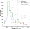
Fig. 1 Histogram for the identified member stars in our sample GCs and OCs (see Sect. 2.1 for details). The distribution for GCs is shown as a dash-dotted red line, for OCs as a dashed blue line, and for the composite sample (GCs+OCs) as a solid green line. The dotted vertical red line with arrows pointing to the right denotes the minimum number of member stars for GCs, and the dotted vertical blue line with arrows pointing to the left indicates the maximum number of identified member stars in OCs.
-
We compute the parameter μR, defined by C18, as:
 (1)
(1)where ⟨μα cos δ⟩ and ⟨μδ⟩ are the median of the proper motion along RA and DEC components, respectively, for data within the chosen ellipse. In short, μR is the distance of every star in the VPD-space to the center of the ellipse.
We plot the G magnitude versus μR and split the magnitude component into 20 bins with bin size of 0.5 mag. In every bin, we compute the median values for G mag and the μR parameter, and the rms (σ) for μR. We then create points with coordinates G median (vertical axis) and μR ± 3 σμR (horizontal axis). We interpolate all the points created in this way and we keep all the values within ± 3 σμR under this interpolation.
We repeat the same procedure as the previous step, but with the parallax (ϖ) instead of μR. For every bin, we create two boundaries with coordinate points-based median G mag (vertical axis) and median ϖ ± 3 σϖ (horizontal axis), interpolate them, and keep the data between these ±3σϖ boundaries.
We iterate this procedure a total of 3 times starting from step 3. For a more detailed description of this procedure, we encourage the reader to view Section 2 and Figure 1 from C18 and Cordoni et al. (2020). Figure 1 shows the distribution of the member stars in our GC and OC sample. We also compared our cluster members with the literature (Dias et al. 2021; Vasiliev & Baumgardt 2021; Hunt & Reffert 2023; Cantat-Gaudin et al. 2020) and found a very good match with them. The small discrepancy in the crossmatch is found mostly towards the fainter magnitudes (G>18). The details of this crossmatch are described in Appendix A.
2.2 Selection of BSSs
We created a CMD ridge-line for each cluster using the median color and magnitude in ∼ 40 bins in the GBP versus GBP – GRP CMD and select MS, subgiant branch (SGB) and red giant branch (RGB) stars. We prefer GBP over the G magnitude in the CMD since it is expected that BSSs will appear brighter at bluer wavelengths across the Gaia SED coverage (see, e.g., Raso et al. 2017). The difference of using G or GBP does not change our final sample size, however, because G covers approximately 330 – 1040 nm, while GBP covers 330 – 640 nm (Rodrigo et al. 2012; Rodrigo & Solano 2020), and given the lack of significant near-IR emission of BSS star the wider coverage of the G filter mainly adds noise and not useful flux information for BSSs (see e.g. D23).
Next, we use PARSEC isochrones (Bressan et al. 2012) that best fit these ridge lines, adopting the stellar population parameters from the literature: For GCs, distances were taken from Baumgardt & Vasiliev (2021), ages from Baumgardt et al. (2023) and extinctions from Harris (2010). All parameters for OCs were taken from Dias et al. (2021), except for two OCs: for Pismin 3 we use parameters from Bisht et al. (2022) and for Trumpler 23 we use parameters from Cantat-Gaudin et al. (2020). Starting from these literature values, we also generate isochrones with slight input parameter variations to explore the best-fit isochrone morphologies: ±0.5 dex in both log (age) and [M / H] in steps of 0.05 dex. With the color excess-extinction relation AV= 3.1 × E(B−V) (see Schultz & Wiemer 1975; Cardelli et al. 1989) converted to Gaia extinction coefficients using the relations AV=1.06794 × ABP and AV=0.65199 × ARP (Marigo et al. 2008; Evans et al. 2018). We consider the PARSEC isochrone that best fits our ridge line for each cluster using a least-square fit.
With the best-fitting isochrones, we divide the data below the MS turn-off (MSTO) point – determined by the infinite slope of the best-fitting isochrone – into 10 bins and record the bin with the largest number of stars. For this bin, we compute its root mean square (rms) along the color axis and call it σcolor. We repeat the procedure, but now for SGB stars, and measure the rms along the magnitude axis to obtain σGBP. To properly select BSSs, we create a region where we shift the best-fitting isochrone 3σcolor to bluer colors and 4 σBP to brighter magnitudes, and adopt an upper cut in magnitude 2 mag above the MSTO for GCs, and 2.5 mags for OCs (Chen & Han 2009; Leigh et al. 2011).
Finally, we recreate a zero-age main sequence (ZAMS) keeping the stellar population parameters for the best-fitting isochrone and shifting it 6σcolor to bluer colors, i.e. twice the quantity we shifted the best-fitting isochrone before. The only 2 differences in the BSS selection between GCs and OCs are in the color selection: (i) for GCs we set a cut in the color up to 0.5 mag to colors bluer than the MSTO to avoid selecting evolved horizontal branch (HB) stars (see, e.g., Culpan et al. 2021). We notice that with this criteria, the selected BSS candidates are found to be located at least five sigma away from the BHB ridge line for all GCs. We did not apply this criterion to OCs, however, because they have no BHB populations. (ii) For OCs, we applied a cut in color to MSTOcolor–3σcolor mag to avoid selecting RGB stars for younger clusters.
Finally, we classify stars within this selection region into 3 types: (i) if they are bluer than the MSTO they are classified as BSSs; (ii) if they are redder than the MSTO and are in the fainter half of the selection region they are classified as yellow straggler stars (YSSs), i.e., evolved BSSs; and (iii) if they are redder than the MSTO and lie in the brighter-half of the selection region they are classified as red straggler stars (RSSs), or evolved YSSs. In this work, we will mainly focus on stars classified as BSSs.
A visual representation of our selection criteria can be appreciated in Figure 2 for two representative clusters, GC NGC 6205 and OC NGC 188, where we display the sample selection results along with their respective VPDs.
We detect 4399 BSSs in our cluster sample. All GCs show BSSs, with a total of 3965 detected BSSs (∼90% of the sample). On the other hand, only 42 out of 129 selected OCs in our sample show BSSs, with a total of 434 BSSs (∼10% of the sample). Comparing our BSS members with the literature, we find that more than 90% of all BSSs are also classified as members in previous studies.
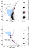 |
Fig. 2 Top: CMD of the GC NGC 6205 using Gaia DR3. Stars that were discarded as cluster members using our selection procedure are shown as gray dots, while cluster members are plotted as black dots. The blue shaded area represents our selection area for BSSs, YSSs and RSSs (see Sect. 2.2) which are shown as blue, yellow and red dots, respectively. The magenta solid curve represents the best-fitting PARSEC isochrone, with the + symbol indicating the MSTO. The right panels show the VPDs for the stars in the respective magnitude range from the left panel. Green crosses represent the median of confirmed members for both components in the VPD. Bottom: same as the top figure, but for the OC NGC 188. We added a red border in the selection area for OCs to avoid AGB/RGB stars (see text for details). |
3 Results and discussion
3.1 Absolute numbers and fractions of BSSs
Figure 3 shows the absolute number (NBSS) of detected BSSs and their number ratio relative to MS stars ( ) in each of our sample GCs and OCs as a function of the parent cluster age. For the denominator of
  , we use the number of MS stars in the luminosity range between the MSTO and MSTO+1 mag, similar to previous studies (JS21, Cordoni et al. 2023). We select MS stars using the same criteria for all clusters shown in the bottom panel of Figure 3 to guarantee a homogeneous comparison. Due to the larger average distances of GCs and therefore, their fainter MSTOs, our earlier photometric depth cut (see Sect. 2.2) collides with the fainter bound of the NMS luminosity range definition for some distant GCs. For this reason we inspected by eye every CMD in our GC sample and only provide
  values for those clusters whose MS stars at 1 mag fainter than the MSTO are within the photometric depth bounds. With this limitation, we are able to obtain
  values for 21 of 41 sample GCs, which is the reason why the number of GCs in the bottom panel of Figure 3 is smaller than the corresponding number in the upper panel. We also list the values of NBSS, NMS and
  in Table D. 1 along with other stellar parameters of the clusters.
The inset panels show zoom-ins at the oldest ages to better visualize any localized trends for the GC subsample. In Figure 3, we also compare the number of BSSs identified in this work against other Gaia-based studies from the literature, i.e. R21, JS21, Li et al. (2023) and Cordoni et al. (2023). We point out that our sample is the first that homogeneously studies BSSs in GCs and OCs. We observe that in all studies, including ours, the BSS population in OCs tends to increase in absolute and fractional numbers towards older cluster ages. This trend appears to reach a maximum at GC ages (log [Age] ≳ 10), however, and it might even be consistent with the numbers of identified BSSs decreasing with increasing age slightly. We also perform sliding histograms of the distributions of (NBSS) and  (dashed line) in Figure 3. NBSS shows a clear trend of increasing with age, while the
  distribution appeared as a plateau in the range log [Age] ≃ 8.9 – 9.5 before suddenly rising again with the varying BSS fraction at older ages. We also perform the Pearson’s r-coefficients in the Monte Carlo method2 (to include observational errors) for both distributions (Curran 2014; Privon et al. 2020)3 and find that the values are
  for NBSS and
  for
for  4. The p-values for both cases are found to be 0. The coefficients and p -values suggest that NBSS and
  , both correlate with the age of the clusters. Although the correlation for
  is moderate, one cannot deny the sudden rise of BSS fraction at log [Age] ∼9.5. The plateau in
  in the range log [Age] ≃ 8.9 – 9.5 could be because, at a young age, massive stars reach larger radii in the AGB phase and mass transfer is possible even in wide binaries, which favours BSS formation to make a constant BSS fraction with respect to the MS population (Leiner & Geller 2021). Other possible mechanisms of more BSS formation are wind accretion from the AGB companion and stable mass transfer in the subgiant branch or Hertzprung gap in younger clusters. The increase in the BSS fractions at older ages might be due to the longer MS lifetime of low-mass BSSs in older clusters and/or the contribution from collisional BSSs, however (Leiner & Geller 2021, see their Fig. 5).
In the inset, we highlight the distribution of  for GCs and compare the trend with that of OCs. We notice that for OCs, as they get older, the
  values increase, whereas for GCs, as they become older, this fraction tends to decrease. We also added a linear fit to the inset plot as a dashed red line that supports this observation. We find the best fit to be:
 (2).
(2).
Pearson’s r-coefficient ( ) suggests, however, that the anti-correlation is rather weak. A similar weak anti-correlation (
 ) is also found for NBSS as well. The p -values are found to be 0 for both cases. As the very central regions of the GCs are excluded in this study because of Gaia’s limitation, incorporating HST observations alongside Gaia data would be beneficial for investigating this correlation. At the same time, we need to include more number of GCs with deep photometry, as we missed to include some GCs due to the magnitude limitation of Gaia.
We note that the dynamic range in  covered by OCs and GCs is similar, unlike the absolute number of BSSs, where GCs show larger absolute numbers due to their larger masses, i.e. more numerous stars. More specifically, GCs show
  while for OCs we find a slightly larger mean ratio of
  .
.
We do not detect BSSs in clusters younger than ∼500 Myr in our sample, supporting the results found by R21, JS21 and Cordoni et al. (2023).
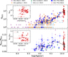 |
Fig. 3 Top panel: absolute number of BSSs vs. age of parent cluster found in this work and other Gaia-based studies. Uncertainties in the BSS number are assumed as Poisson errors. The inset sub-panel shows a zoom-in on the GC age range for better visualization. The dashed black line denotes the “ridge-line” based on the sliding histogram (see text for details). Bottom panel: ratio of BSS numbers relative to the number of MS stars in the luminosity range between MSTO and MSTO+1 mag (see Sect. 3.1). We compare the ratio against those studies that also provide this parameter with the same criteria for MS stars number selection, if available. From the considered studies (see legend), only R21 and Cordoni et al. (2023) have this parameter available. Data based in our work is plotted only for those GCs whose NMS is not cut by the photometric depth selection described in Section 2.1; this is done to guarantee a consistent comparison between different clusters and samples. For the uncertainty in NBSS/NMS we assume a simple error propagation with Poisson errors for MS stars and BSSs. Errors in age for GCs are based on the difference between our best-fitting isochrone models and those derived from Baumgardt et al. (2023), whereas errors in ages for OCs are taken from Dias et al. (2021). Similar to the top figure, the black-dashed line represents the “ridge-line” based on the sliding histogram. |
3.2 Astrophysical parameters of BSSs
We derive the following astrophysical parameters for our sample BSSs: effective temperature (Teff), stellar mass (M), luminosity (L) and surface gravity (log g). We used three different approaches: the infrared flux method (IRFM; from colortemperature relations), the isochrone best-fit method (from PARSEC isochrones) and the XPP from Gaia DR3 spectra, if available. While the isochrone method provides all astrophysical parameters, the IRFM method provides Teff and the XPP method gives Teff & log g. We mainly use the parameters obtained from the isochrone method, but it is necessary to compare Teff values, obtained from all three methods to check the consistency in the parameter estimations. In Appendix B, we describe all three methods and the comparison of the Teff values obtained from them, in detail. In the following subsections, we summarize the results and compare the stellar parameters with the literature values.
3.2.1 Effective temperature
We notice that Teff values extracted from different approaches range from ∼6000 K to 9000 K and appear consistent with each other with a little systematic offset towards higher temperature (Teff > ∼8000 K). From these comparisons, we estimate that the systematic uncertainty between various methods is of the order ΔTeff ≃ 100 K. From the IRFM we find ⟨Teff, IRFM⟩=(6772 ± 630) K for GCs and ⟨Teff, IRFM⟩=(7598 ± 1476) K for OCs. From isochrone fitting we find ⟨Teff, isochrone⟩=(6829 ± 529) K for GCs and ⟨Teff, isochrone⟩=(7549 ± 1331) K for OCs. Only 537 of 4399 BSSs (∼12% of our sample) have XPP parameters measured for 279 stars in GCs and 258 stars in OCs. With this method, we find the mean BSS effective temperature of ⟨Teff, XPP⟩=(7271 ± 732) K for GCs and ⟨Teff, XPP⟩=(7269 ± 1331) K for OCs. We list these parameters in Table D.2, and the full table is available at the CDS.
Table 1 compares our derived values for Teff with those found in the literature for various OCs and GC, as well as BSS samples. We find that our effective temperatures derived are in very good agreement with previous studies. For example, Jadhav et al. (2019), Sindhu et al. (2019) and Pandey et al. (2021) have analyzed different BSSs in the OC NGC 2682 (also known as M67) by fitting models to spectral energy distributions (SEDs) searching for BSS hot companions; these studies derive BSS temperatures in the range between 6510 and 8300 K, which are in excellent agreement with our measurements, yielding a mean Teff=7300 ± 1000 K for all methods combined. We also point out the excellent agreement with the Teff values derived in Gosnell et al. (2015), where the authors find ⟨ Teff⟩=6396 ± 23 K for 19 BSSs, which is in very good agreement with our results independent of the applied method (6366 ± 49 K and 6473 ± 41 K, for the IRFM and isochrone method, respectively). Finally, our ⟨ Teff⟩ ≈ 6800 K is also in very good agreement with theoretical predictions for BSSs in GCs from Stępień & Kiraga (2015) who calculate ⟨ Teff⟩=(6969 ± 96) K, and who had applied different initial conditions to binary systems.
3.2.2 Stellar mass and age of the BSSs
Stellar mass and age are important parameters in the study of the evolutionary state of BSSs. We derive these parameters along with equivalent stellar luminosity and stellar surface gravity for all BSSs in our sample based on the isochrone fitting method. We obtain the mean luminosity ⟨log (LBSS / L⊙)⟩= 0.58 ± 0.21 for GCs and ⟨log (LBSS / L⊙)⟩=1.13 ± 0.44 for OCs, and find the mean surface gravity of ⟨log (gBSS /[cm · s−2])=. 4.14 ± 0.22 for GCs and ⟨log (gBSS /[cm · s−2])=3.98 ± 0.21. for OCs. These values correspond to a mean stellar mass ⟨ MBSS⟩= 1.02 ± 0.1 M⊙ for BSSs in GCs and ⟨ MBSS⟩=1.75 ± 0.45 M⊙ for BSSs in OCs, which altogether translates to a mean stellar age of log (AgeBSS / yr)=9.586 ± 0.318 for BSSs in GCs and log (AgeBSS / yr)=9.065 ± 0.344 for BSSs in OCs.
We compare these values with previous results from the literature in Table 1. We find that the average mass of our BSS sample in GCs (⟨ MBSS, GC⟩=1.02 ± 0.1 M⊙) differs from previous works, which report ⟨ MBSS⟩=1.7 ± 0.4 M⊙ (Shara et al. 1997) and ⟨ MBSS⟩=1.22 ± 0.12 M⊙ (Baldwin et al. 2016). This may be partly explained by the lower BSS numbers of previous studies, but also by either of the previous arguments, i.e. i) limitations of the Gaia data selection and ii) BSS mass segregation in GCs. In particular, the latter argument lends credence to the reason for this offset as the two previous studies are based on HST observations that target the GC centers. Our sample, on the other hand, is based on BSS samples from outside the half-light radius. Nevertheless, as can be appreciated in Table 1, our BSS mass results are in very good agreement with those measured by Simunovic (2017,⟨ MBSS⟩=1.07 ± 0.13 M⊙), Fiorentino et al. (2014, ⟨ MBSS⟩=1.06 ± 0.09 M⊙) and Stępień & Kiraga (2015, ⟨ MBSS⟩ ≈ 1 – 1.1 M⊙). The comparison with Simunovic (2017) is in particular striking, as this work measured the parameters for 1507 BSSs in 38 GCs using the isochrone fitting technique similar to our procedure, which makes it statistically the most robust comparison.
The average BSS mass for our OC sample ⟨ MBSS, OC⟩= 1.75 ± 0.45 M⊙ compares favorably with the corresponding value found by JS21 considering the uncertainties. They report an average mass value of ⟨ MBSS, OC⟩=2.67 ± 1.2 M⊙ if only confirmed BSSs from their catalog are considered, and ⟨ MBSS, OC⟩= 2.49 ± 1.13 M⊙ if both confirmed and candidate/probable BSSs listed in their catalog are included. As was explained previously, the difference between these works is likely the result of our Gaia G magnitude cut-off criterion, discarding all bright stars with GBP ≤ 10 as they are likely saturated and therefore, their Gaia parameters likely affected by systematic errors. This not only explains the difference between our results, as well as why our dispersion in BSS mass for OCs is smaller, but also the lack of BSSs younger than ∼500 Myr in our sample, most of which would naturally be among the most massive BSSs.
3.3 Effective temperature versus cluster age
In Figure 4, we compare the average MSTO offset in Teff of BSS in a cluster against the corresponding cluster age. To compare self-consistently all the BSSs with respect to the same evolutionary reference point, given the clusters’ very different ages and metallicities, we use the Teff of their MSTO as a reference. For each BSS, we obtain Δ Teff=Teff, BSS−Teff, MSTO. We then compute ⟨Δ Teff⟩ which is the mean difference between the BSS temperatures and the Teff, MSTO in each cluster. As XPP parameters are not available for stars at the MSTO, we only do this for Teff obtained by isochrones and color-temperature relation, i.e. IRFM, and recall the systematic offsets found in the comparison of these methods (see Fig. B.2). The error bars in Δ Teff represent the dispersion of BSS temperatures in each cluster, while the error bars on the horizontal axis are age uncertainties.
Comparison between BSS astrophysical parameters obtained in this study against those found in the literature.
In the top panel of Figure 4, BSSs in OCs show on average a trend against the parent cluster age where younger OCs show larger ⟨Δ Teff⟩ offsets, i.e. hotter BSSs, with respect to those found in older OCs, or in other words, the difference between the effective temperature of BSSs and the MSTO effective temperature decreases with increasing parent cluster age. Pearson’s coefficients for IRFM (isochrone) method is  (
( ), suggesting the correlation to be weak, which could be due to a large dispersion in the BSS temperatures in the younger cluster. We expect the observed trend, however, because younger clusters host more massive stars which are also larger in diameter (e.g. Iben 2013), and therefore, have likely more efficient MT between binary members and higher collision/capture probabilities with other stars. These hotter BSS stars evolve faster than BSS stars around the MSTO and, thus, the difference in average Teff between BSSs and BSSs around MSTO is expected to decrease with time. We also notice that the dispersion in Δ Teff decreases with the age of the OC, which may indicate that BSSs tend to be more concentrated in the colorluminosity space as the OC ages, which is also shown in the bottom panel of the figure. Pearson’s coefficient values further confirm the trend:
  and
and  for IRFM and isochrone methods, respectively.
We do not observe any of these correlations for BSSs in GCs, which is also supported by the Pearson’s coefficient for the IRFM (isochrone) method  (see inset panels in Fig. 4). We recall, however, that we might be exposed to biases for the GC subsample: (i) we applied a color cut when selecting BSSs in GCs to avoid including BHB stars (see Fig. 2 and Sect. 2.2) which, although unlikely may cut into the distribution of BSSs with extremely large Δ Teff (this could in principle be tested with UV photometry); (ii) Gaia is only capable to observe stars outside ∼ rhl (half-light radius) in GCs, which could change the mean Δ Teff if we assume that mass segregation has already acted on the BSS population (Contreras Ramos et al. 2012; Ferraro et al. 2012). Without consideration of these potential biases and taking the distributions in Figure 4 at face value, this means that as GCs age past ∼10 Gyr, BSSs are more or less equally distributed in Δ Teff.
In the middle panel of Figure 4, we check if the fractional ⟨Δ Teff⟩ excess with respect to Teff, MSTO has any correlation with the cluster age. We do not find any trend for either OCs or GCs, which is also supported by the Pearson’s coefficient test. Pearson’s coefficients for IRFM (isochrone) are  for OCs and
  .
.
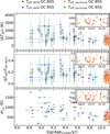 |
Fig. 4 Teff vs. cluster age. Top: ⟨ Teff⟩ – the mean of the difference between BSS Teff and MSTO Teff, found with the same method, for stars within the same cluster – vs. cluster age. Blue triangles and red dots represent Teff obtained from color-temperature relations for OCs and GCs, respectively. Green plus symbols (+) and orange squares represent Teff derived from isochrone models for OCs and GCs, respectively. At the top right corner we show the results only for GCs without error bars for a better appreciation, keeping the same axes from the major plot. Error bars along vertical axis show the dispersion of BSSs Teff. Middle: difference between ⟨ Teff⟩ and the MSTO Teff, normalized by the MSTO temperature. Horizontal gray dashed line indicates BSS Teff=1.5 × MSTO Teff. Bottom: dispersion of BSS Teff vs. cluster age. |
3.4 Fractional mass excess of BSSs
Blue straggler stars are expected to gain mass during their MS lifetime. This means that the ”excess“ between their current mass and the stellar mass at the MSTO could provide hints about their formation pathways. Recall that, based on previous observations (Dalessandro et al. 2013; Dattatrey et al. 2023), hotter (bluer), but relatively faint BSSs are likely to be formed through collisions, whereas slightly cooler (redder), but slightly brighter BSSs are likely to be formed by MT. Even though this is almost certainly not strictly followed by the universe (modulo stellar-mass loss rate, binary parameters, environmental factors, such as tidal shocks and disruption of binaries, etc.), it could be considered a first scenario for the formation of particular BSS subpopulations. Trying to provide a quantity that could give a hint which pathway dominates certain evolutionary phases, JS21 defined a parameter called the “fractional mass excess”, or  . This quantity is defined as
 (3)
(3)
where MBSS is the mass of the BSS and MMSTO is the stellar mass at the MSTO, which in our case is obtained from isochrone models. In simple words,  is the excess between the BSS mass and MSTO mass, normalized by the MSTO mass. Note that
  is equivalent to MBSS=1.5 × MMSTO, and
  corresponds to MBSS=2 × MMSTO. By definition, this “fractional mass excess” is roughly equivalent to the MT efficiency if we assume that both member stars of the system, the donor and the secondary star, are MS stars (Shao & Li 2016). JS21 decided to divide the
  range into three ad-hoc regimes: low
  , high
  and extreme
  where, as a first approximation they speculated, different BSS formation pathways would dominate, which are MT, stellar collisions, and multiple-mergers/MT, respectively.
To make headway in the discussion of BSS formation pathways, we study the behavior of  as a function of cluster age and the equivalent BSS age from isochrone fitting, both of which are displayed in Figure 5 along with the BSS mass and mass offset scalings. We focus first on the left-side panel. In the top panel, we observe that, as expected, younger clusters host BSSs with higher masses, which decrease with cluster age. The Pearson coefficient also provides a strong correlation value of
  , combining both OCs and GCs. This correlation is consistent with the decreasing MSTO mass as a stellar population ages, since the lifetime of a star, τ, scales as
  , i.e. more massive stars have M−3 shorter lifetimes compared to less massive stars, which translates into the BSS mass relation in the top left panel of Figure 5. This correlation also appears stronger when only OCs are considered
  , but this is not true for the GC sample
  . The reasons for GCs are the same as discussed in the previous sections.
The middle panel on the left side of Figure 5 shows the difference between the BSS mass and the MSTO mass as a function of cluster age. We see that the BSS with higher mass difference are absent towards the older cluster age with Pearson coefficient of  . This is also expected from regular stellar evolution since more massive stars end their life disproportionately earlier while the MSTO mass decreases more slowly with increasing age, which is exactly what is observed, i.e. Δ M=MBSS−MMSTO shrinks as time advances. We also notice here that GC sample alone does not show any correlation (
 ).
).
More surprisingly, we find no trend of  with cluster-age (bottom left panel in Fig. 5) either for OCs or GCs with Pearson coefficient values
  and
and  , respectively. We observe, however, that the fraction of high-
  BSSs is larger in OCs (18.7%) compared to GCs (5.8%), which may indicate that the collisional formation channel is more pronounced in younger star clusters. This in turn might be related to sufficiently old dynamical ages of star cluster, which can, in principle, have undergone one or more core collapse, boosting the stellar encounter rates, and therefore, the formation of collision-induced BSS formation. This might be accomplished for star clusters with ages of a few billion years, however, and it requires further investigation and modeling. We find 81.3% and 18.7% as the BSS fractions with low and high-
  (split at
  ), respectively, for OCs. In GCs, we find these proportions to be 94.3% and 5.8% for low- and high-
  , respectively. Considering all clusters, the percentage of low-
  is 93% and for high-
  we obtain 7%.
Additionally, we plot the BSS mass parameters versus BSS ages in the right panels of Figure 5. The relations for MBSS and Δ M are consistent with those found against the cluster age (left side of the same figure), i.e., both of these parameters decrease as a function of BSS age and stellar population age. In addition, we see various sequences that indicate that the BSSs in OCs and GCs predominantly populate different parameter spaces. A striking distribution is found in the  against log (BSSs age) plot (bottom right panel) which shows two dominant sequences, both of which are consistent with decreasing
  as BSSs become older, albeit at different rates. We will later show that these sequences are likely representative of the different BSS formation channels. The Pearson coefficients for all these three relations for OCs (GCs) are:
  for MBSS versus BSS ages;
  for Δ M versus BSS ages; and
  for
for  versus BSS ages.
Figure 6 shows the percentage of low-  and high-
  BSSs as a function of BSS age. For OCs, it is clear that the high
 fraction vanishes above the BSS ages of ∼2 – 3 Gyr, whereas the low-
  fraction dominates, with a percentage >90% in the same older age range. Curiously, the high-
  fraction in GCs increases to ∼30% for BSS ages between ∼1.5 – 2.5 Gyr, while the low-
  fraction experiences a corresponding dip. This may be due to the predominance of BSS formed through the collisional channel at those ages. Ferraro et al. (2009); Dalessandro et al. (2013); Simunovic et al. (2014) fitted collisional isochrones (Sills et al. 2009) to the blue sequence of BSSs, finding that their ages are ∼2 Gyr, concluding that double sequences of BSSs in GCs may be products of violent interaction episodes in the past core-collapse events, which is in agreement with our age range found for BSS in GCs where the high-
  fraction increases and the low-
  fraction dips. For GCs older than ∼3.5 Gyr the high
  fraction rapidly vanishes similar to those for OCs. Overall, we observe that for all BSSs in our sample low/high-
  total fraction is dominated by OCs for younger BSSs ages (∼250− 600 Myr) and by GCs for older BSSs ages (∼1.5 – 10 Gyr) as expected by their sample characteristics (see Sect. 3.1).
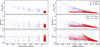 |
Fig. 5 Mass of BSSs. Left: mass of BSSs (found with isochrone models) vs. parent cluster age. Upper panel shows the mass of the BSSs, the middle panel shows the difference between the BSS mass and the MSTO mass, and the lower panel shows the mass excess factor, |


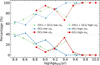 |
Fig. 6
|


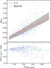 |
Fig. 7 Comparison for |


3.5 Comparison with JS21
In Figure 7, we compare our measured  values against those from JS21. In the upper panel, the dashed red-line shows the 1-to-1 relation, whereas the yellow solid line marks the best linear fit, with the shaded area representing the 95% confidence interval. Overall, we point out that our values are slightly larger compared with those provided by JS21, as can be appreciated in the inferior panel of Figure 7. An explanation is our Gaia DR3 selection criteria, due to the 10.5 mag ≤ G ≤ 19.5 mag magnitude selection. We skipped too bright/saturated stars to avoid systematics, which may have been classified as more massive (very bright) BSSs by our models, especially in OCs. In addition, the systematics slope and scatter in Fig. 7 are in part due to JS21 measuring BSS masses using a different isochrone approximation from ours, i.e. for every BSS they estimate its magnitude position on the ZAMS and compute its mass based on this model, not on the best-fit isochrone like in our approach.
We recall that JS21 classified BSSs into three classes, i.e. low-  , high-
  and extreme-
  objects, which are speculated to predominantly form via MT, stellar collisions, and multiplemergers/MT, respectively. In addition to our direct comparison of OCs and GCs, the difference between our results and those provided by JS21 is that we were unable to find any stars with
  in the extreme-
  regime, most likely due to our Gaia photometry cuts. It is important to mention, and as JS21 have warned, that the “fractional mass excess”
  does not strictly indicate how BSSs are formed, but it rather suggests how BSSs may likely be formed. For a deeper analysis, which escapes the Gaia limitations, we do need FUV observations to be able to distinguish the presence or absence of hot companions (e.g. Subramaniam et al. 2016; Sindhu et al. 2019).
We plot the distribution of low- and high-  BSSs in OCs and GCs in the Gaia CMD shown in Figure 8, similar to JS21 (see their Fig. 6). We find that BSSs in OCs and GCs classified as high-
  show a modest difference in color, being bluer than low-
  BSSs by ∼0.2 mag. The more significant difference is in the absolute magnitude where high-
  BSSs are, on average, approximately 10 times brighter than low-
  BSSs. This difference is appreciable for both types of clusters, GCs and OCs. Although this empirical classification resembles the instantaneous mass excess with respect to the MSTO, it does not resemble the classic evolutionary pathways of stars, which leads them from the MS to the colder subgiant branch and then up the RGB.
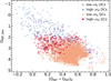 |
Fig. 8 Gaia photometry color-magnitude diagram for BSSs classified by their |


3.6 Toward evolutionary pathways of BSSs
With the goal of advancing our understanding of the BSS formation channels and capturing the predominance of the BSS formation channels, we combine the fractional mass excess parameter (Me) with our earlier derived equivalent BSS ages. We focus our attention on Figure 9, the upper panel of which reproduces the bottom right panel of Figure 5, but this time, we separate the two sequences 5 into a high-mass excess sequence and low-mass excess through the next procedure:
For the identified BSSs, we separate them using as criteria if they belong to an OC or a GC and make a plot
 versus log (Age.BSS/yr) (similar as the bottom-right panel of Figure 5).
-
We then set two edges by eye that enclose all the points in this plane. We define an inferior and superior edge, which is different for OCs and GCs. For OCs we define the lower edge defined as:
 (4)
(4)
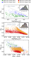
Fig. 9 Top:
 vs. BSS age (found with isochrone models) for OCs. Middle:
  vs. BSS age (found with isochrone models) for GCs. In both Top and Middle panels, the dashed gray lines used to separate the BSSs classified as “upper” or “lower” sequences. OC BSSs and GC BSS that are tagged as “upper” sequence BSSs are symbolized by blue triangles and yellow squares, respectively. “lower” sequence for OCs and GCs are represented by green plus (+) symbols and red dots, respectively. Bottom: CMD (using absolute magnitudes and de-reddened colors) based on BSSs sequence tag. Symbols are the same as the top figure.
where x=log(AgeBSS/yr) is the BSS age found with isochrone fittings. We then define the superior edge for OCs as
 (5).
(5).In a similar way, we computed these edges for GCs as
 (6)
(6)and
 (7)
(7) To check the distribution along the horizontal axis, for every point j from OCs in this plane with coordinates (
 ), we compute the distance between the point and its superior edge along the vertical axis and normalize this value by the distance between the superior and inferior edges to “flatten” it. We can reach this using the expression
 (8)
(8)We repeated the last step, but this time for BSSs from GCs using the respective edges values from step 2.
We fit a bimodal distribution using SciPy (Virtanen et al. 2020) to the distance distribution obtained with equation (8) for OCs and GCs, separately.
Based on the values that optimize the bimodal distribution for the discovered distances, we compute the probability density function (PDF) of each Gaussian and estimate the membership probability of each point to be a member of each Gaussian.
If the point has a higher probability to belong to the Gaussian with lower distances, this means that the point belongs to the distribution that is closer to the superior edge, and it is therefore classified as a member of the “upper”
 sequence. Else, they are classified as a member of the “lower”
  sequence.
To properly compare BSSs with this new classification scheme, we plot them in a Gaia photometry CMD in the lower panel of Figure 9 (bottom panel), which can be directly compared to Figure 8 which encodes the  classification from JS21. Our new classification now resembles more the expected stellar evolutionary pathways of BSSs, clearly separating the BSS population in GCs into two dominant sequences. We also observe that the upper-
  sequence BSSs in OCs predominantly populate the brighter sequence of OC BSSs in the CMD. In general, we find that the color range covered by the two
  sequences is similar for GCs and OCs, but there is a systematic offset in luminosity with the upper-
  sequence BSSs appearing about 1 mag brighter than their lower-
  sequence counterparts.
In the following, we briefly explore possible explanations and considerations when interpreting these clearly distinct BSS sequences.
3.6.1 Mass transfer evolution
From a binary evolution perspective, the upper-  sequence may represent a BSS population that was formed through more efficient MT processes. This would imply more accreted mass and, hence, more fuel on the receiving star, accelerating its evolution (McCrea 1964). Assuming this scenario and a subsequent common-envelope evolution, the separation between the stars of such a binary system will eventually decrease until the final stages which could play out in two scenarios: (i) the cores could merge or (ii) one of the cores could be ejected from the system through interactions with envelope and/or other stars. The former scenario is more likely (Hurley et al. 2002). The result of a stellar merger is a massive BSS, which would experience fast subsequent stellar evolution (τ ∝ M−3) and be more likely encountered at older BSS ages. We therefore interpret the two sequences in the
  versus log(Age.BSS/yr) plane as post-merger/close-binary interaction sequence (“upper” sequence) and pre-merger/closebinary interaction sequence (“lower” sequence, see Fig. 9).
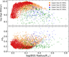 |
Fig. 10 log(AgeBSS) and |

3.6.2 Unresolved binary stars
It is trivial that some BSSs may be unresolved binary systems (Gosnell et al. 2015; Subramaniam et al. 2016; Sindhu et al. 2019). When we fit isochrone models to our BSS sample, however, we implicitly assumed a single-star evolution. Jiang (2022) has shown through multiple simulations that the total mass of the system is higher in unresolved MT binaries compared to post-MT BSSs by about 0.2 – 0.6 M⊙. This means that the isochrone fitting method could be overestimating ages and underestimating the masses for unresolved MT BSSs, located preferentially in CMD regions with similar colors as the MSTO and the subgiant branch. Therefore, the upper-  sequence could be stars with an overestimated age – showing higher
  values – since they are unresolved MT binaries, while the lower-
  BSSs could be post-MT binaries whose companions either have negligible mass or which are in the post-MT phase.
3.6.3 Effect of variations in the stellar radius
As rejuvenated stars evolve of the ZAMS towards the subgiant branch and are therefore expected to grow in size, we compute the radii of our sample BSSs, R, using the relation  , where G is the gravitational constant, M is the stellar mass and g is the surface gravity. We assume g in cgs units (from isochrone models) and stellar mass in M⊙ units, computing the value of R in solar radii using Astropy routines (Astropy Collaboration 2013). We show the results in Figure 10:
  and log(AgeBSS) as a function of stellar radius (R). We note that after adding stellar radius, the separation between upper- and lower-
  sequences is even more pronounced for GCs.
This is consistent with the expectation of an evolved binary system for BSSs in the upper-  sequence (orange squares in Fig. 10), where the system might be in the common envelope phase. Such systems evolve rapidly and reach subsequent stages with similar characteristics of an SGB or RGB star, where they begin the radial expansion, which qualitatively agrees with our observations. We were unable to identify any clear difference between the upper- and lower-
  sequences for BSSs in OCs, however, which may be an indication of a different mix of BSS formation mechanisms acting in lower mass, lower density star clusters. We defer the detailed modeling of these systematic differences between OCs and GCs to future work.
4 Conclusions
With the new  −log(AgeBSS/yr) classification scheme of BSSs, we inspected the CMDs of all our sample GCs and OCs individually to determine whether the BSS subpopulations are differentiated by our classification in the color-magnitude space. We observed that BSSs classified as upper-
  members are brighter and that lower-
  sequence member stars appear fainter. In Figure 11 we presented the distribution of upper- and lower-
  sequence BSSs in the representative GC NGC 362 and OC Berkeley 39. We also overlaid isochrones corresponding to the ZAMS and binary ZAMS. The figure shows that binary ZAMS passes through the majority of the BSSs that intersect the upper- and lower-
  sequence, while the ZAMS passes through a smaller fraction of the lower-
  sequence (red points). The lack of BSSs on the ZAMS also suggests the lack of collisional BSSs, which is also expected because NGC 362 is a core-collapse GC and the Gaia data are unable to resolve the core of the GCs. We do not expect to observe collisional BSSs in OCs either because the environment is not dense enough to favor collision. Our classification is not similar to the literature classification of blue and red BSSs sequences observed in corecollapse GCs, where blue BSSs are thought to form through direct collisions and the BSSs in the red sequence are thought to form via MT (Ferraro et al. 2009; Dalessandro et al. 2013). We note that blue (or collisional) BSSs are dominated by our lower sequence, whereas the red sequence is a mix of the upper and lower sequence. Our new BSSs classification based on
  log(AgeBSS/yr) mainly highlights the pre- and post- merger/MT scenarios of the BSSs. Our study suggests that companions in our
  classification may imply that most of our stars that are classified as upper-
  sequence BSSs might be consistent with the presence of a companion, while lower-
  BSSs may preferentially indicate post-MT/merger-product BSSs. This may support our hypothesis, which assumes that we might be overestimating the ages of BSSs because we cannot resolve the binary system, and therefore, the BSSs were classified as upper-
  sequence members.
The distribution of upper- and lower-  sequence BSSs in the CMDs for GCs and OCs is similar for all clusters. The CMDs of all the clusters highlighted with these two sequences are made available on Zenodo for reference. In some of the clusters (NGC 104, NGC288, NGC 2808, NGC 3201, NGC 5139, and NGC 6121) that are not classified as core-collapse GCs, we observed that a significant number of BSSs are located on the ZAMS or are bluer than the ZAMS. These most probably formed through a direct collision or post-MT/merger, as suggested by the literature on core-collapse GCs. The significant number of BSSs outside the core or half-light radius of the clusters makes these GCs interesting candidates and requires a further detailed analysis to interpret the observed nature.
Much more theoretical work and observations are required to elucidate whether and to which extent our new classification scheme of BSSs resembles the formation and evolution mechanisms of these unique stars. We summarize the results and conclusions of our work below:
We selected OCs from Dias et al. (2021) with more than 350 star members and GCs from Vasiliev & Baumgardt (2021) with more than 1000 star members to ensure well-sampled cluster stellar populations, and we used data from Gaia DR3, for which we adopted an algorithm based on prescriptions from C18 and Cordoni et al. (2020) to extract cluster members;
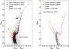
Fig. 11 CMD for BSSs classified as “upper” and “lower” sequences, based on sequences shown Figure 9, for GC NGC362 and OC Berkeley 39. ZAMS and ZAMS – 0.75 mags are displayed as a purple dashed line and as a green dash-dotted line, respectively. Orange plus (+ symbol) and magenta line represent the MSTO and the best-fitting PARSEC isochrone, respectively (similar to Figure 2). Field/non-member stars are displayed as gray points, whereas confirmed members are displayed as black points. BSSs that lie in the upper-sequence and lower-sequence are symbolized as orange squares and red dots, respectively.
Using the confirmed cluster members, we fit PARSEC isochrones (Bressan et al. 2012) to obtain parameters such as the age for every cluster in our sample;
Using the ridge line of the observed CMD and the best-fit isochrone found in the previous step along with the ZAMS and the dispersion of stars along these sequences, we defined a BSS selection. We were able to find BSSs in all our sample GCs and in 42 out of 129 (∼33%) OCs of our sample. We identified a total of 4399 BSSs, 434 of which (∼10%) are located in OCs and 3965(90%) are located in GCs;
We extracted astrophysical parameters for all identified BSSs using three different methods: 1) color-temperature relations (i.e., IRFM), 2) model isochrone fitting, and 3) parameters from Gaia DR3 spectra from Zhang et al. (2023, called XPP), if available. From the color-temperature relations, we only obtained Teff. From the isochrone fitting, we obtained Teff, log g, log L, stellar masses, and ages. From XPP we obtained Teff and log g;
We found no BSSs in clusters younger than ∼500 Myr;
We found effective temperatures for BSSs ⟨ Teff⟩=6853 ± 795 K from the color-temperature relations and ⟨ Teff⟩= 6900 ± 687 K from the isochrone fitting for our entire BSS sample. The Teff found in OC BSSs are ⟨ Teff⟩= 7598 ± 1476 K and ⟨ Teff⟩=7549 ± 1331 K from the colortemperature and isochrone-fitting methods, respectively. The BSSs in GCs present slightly lower temperatures, with ⟨ Teff⟩=6772 ± 630 K derived from color-temperature relations and ⟨ Teff⟩=6829 ± 529 K from isochrone models. Overall, the difference in Teff found from isochrone fittings is that they are ∼50 K hotter than those obtained from color-temperature relations. These values agree with those of previous studies;
Based on the isochrone-fitting method, we determined that the average mass of all our BSSs is approximately ⟨ MBSS⟩= 1.09 ± 0.28 M⊙. The average mass of BSSs in OCs is at ⟨ MBSS⟩=1.75 ± 0.45 M⊙. We obtained an average BSS mass for GCs of ⟨ MBSS⟩=1.02 ± 0.1 M⊙. Our average mass for BSSs in OCs is lower than the mass determined by JS21, which is likely due to our more conservative selection, but they still agree within their respective error ranges. Our results agree very well with most other studies;
We compared Teff against its counterpart measured at the MSTO of the parent cluster. Regardless of the method we applied, we found for OCs and GCs that the difference between the mean BSS Teff and the MSTO Teff decreases with the cluster age. This is in line with expectations from stellar evolution because massive stars evolve faster than stars at the MSTO. The Teff dispersion in OCs decreases with the cluster age. We did not find this last relation in GCs, which means that the Teff dispersion of BSSs does not depend on the cluster age in GCs;
We followed the definition provided by JS21 for the fractional mass excess, or
 . This parameter quantifies the difference between the BSS mass and the stellar mass at the MSTO (this last based on isochrone fittings), normalized by the MSTO mass.
  is roughly equal or proportional to the MT efficiency in a binary system. These authors classified
  into three regimes, each assumed to be dominated by a specific BSS formation pathway: i) low-
  , likely to be formed via MT), high-
  , likely to be formed through mergers or collisions), and extreme-
  , likely to be multiple MT systems). In our sample, we found no extreme-
  , which is likely to be due to the conservative selection, where we avoided stars brighter than GBP ≲ 10 (to avoid Gaia systematic errors), which may contain some more massive BSSs. In our final BSS sample, 7% are classified as high-
  and 93% as low-
  . This proportion is ∼81.3% and ∼18.7% for low −
 and high −
 , respectively, for OCs. For BSSs in GCs, we found these percentages to be ∼94.3% for low-
  and ∼5.7% for high −
 . This suggests that mass transfer is the most likely formation channel for BSSs, but OCs show a higher fraction of high-
  BSSs, some of which may have formed through mergers as well;
Finally, we explored a new BSS classification scheme that uses
 versus log(AgeBSS). This parameter space shows a clear double sequence for BSS in GCs: One parameter space corresponds to an upper sequence, with higher
  as a function of the BSS age, and another lower sequence that is linked to lower
  as a function of the BSS age. We plotted the BSSs labeled according to this classification scheme in the Gaia CMD and found a clear division between these branches, especially for GCs. BSSs on the upper-
  sequence are brighter than those located on the lower-
  sequence. We explored two possible explanations: 1) In binary star evolution, mass transfer increases the mass of the receiving star and in the process decreases the distance between the binaries, while the receiving star begins an accelerated evolution and therefore appear as an older star in the isochrone tracks. In this scheme, these upper- and lower-
 sequences are consistent with post-merger or close-binary interaction and pre-merger binary evolution. 2) We might be overestimating the age and underestimating the mass of the upper-
  sequence BSSs because we assumed single-star evolution during the isochrone fitting. Therefore, the upper- and lower-
  sequences may be equivalent to an overestimated and realistic BSSs age, which could be correlated with the presence (or absence) of a BSS companion. Further observations targeting various parameters, such as the stellar rotation speed statistics, chemical compositions, and binarity, are required to shed light on this intriguing new bifurcation in the
  versus log(AgeBSS) classification.
Data availability
Parameters of BSSs, YSSs, RSSs and the star clusters presented in this study (full Tables D.1 and D.2) are available at the CDS via anonymous ftp to cdsarc.cds.unistra.fr (130.79.128.5) or via https://cdsarc.cds.unistra.fr/viz-bin/cat/J/A+A/699/A142 and on Zenodo for reference.
Acknowledgements
P.K.N. and T.H.P. acknowledge support by the ANID BASAL projects FB210003. T.H.P. gratefully acknowledges support through the FONDECYT Regular Project No. 1201016.
Appendix A Validation of our membership criteria
To validate our BSS membership criteria as well as all other cluster members, we compare our cluster members with the literature. We only compare the clusters which show the presence of BSSs as we only focus on these clusters in our further analyses. The most recent and extensive membership catalogs using Gaia data are given by Vasiliev & Baumgardt (2021); Hunt & Reffert (2023) for GCs and Cantat-Gaudin et al. (2020); Hunt & Reffert (2023) for OCs. Vasiliev & Baumgardt (2021) provided membership probability of all stars in 170 GCs using the Gaussian mixture model on Gaia-EDR3 data, where stars with a membership probability greater than 90% are considered to be cluster members. We find more than 90% matches in membership for all 41 GCs, with a median crossmatch accuracy of 99.7%. All BSSs detected in our GCs sample are also classified as cluster members in Vasiliev & Baumgardt (2021). Hunt & Reffert (2023) used HDBSCAN algorithm on Gaia DR3 data down to magnitude G ~ 20 mags to recover 7167 clusters, including 134 globular clusters. For GCs, we find that the crossmatch between our catalog and Hunt & Reffert (2023) varies from 15% (for NGC 6656; very close to the Galactic plane) to >95% based on the distance of the clusters from the Galactic plane, with a median crossmatch accuracy of 84%. NGC 104 is not studied by Hunt & Reffert (2023), hence we are unable to make any crossmatch with this cluster. The membership method of Hunt & Reffert (2023) is found to have a bias on whether the cluster is located in a crowded or sparse field, which is not found in the methods of Vasiliev & Baumgardt (2021). In Figure A.1, we show CMDs of two GCs (NGC 3201 and NGC 288) to demonstrate the comparison of the cluster membership obtained from our method (blue), Vasiliev & Baumgardt (2021) in orange and Hunt & Reffert (2023) in green. The figure shows a good agreement between all three methods.
We find a better crossmatch with Hunt & Reffert (2023) for OCs. We find a crossmatch of more than 50% for all clusters (except UBC252 with 19%) and with median crossmatch value of 94%. The unmatched sources are mainly fainter than ∼18 mags in G band and more importantly, all BSSs in our sample are also classified as cluster members in Hunt & Reffert (2023). Dias et al. (2021) used the classic maximum likelihood approach (Dias et al. 2014; Monteiro et al. 2020) on Gaia-DR2 data to study ~2000 open clusters for stars brighter than 18 mags in the G band. The comparison shows that the crossmatch fraction varies from 60% to 96% with a median value of 88%. The difference in the crossmatch is mainly found towards the fainter G magnitudes. When cross-matched only with our BSS sample, we find more than 97% are also classified as members in Dias et al. (2021). Cantat-Gaudin et al. (2020) applied an artificial neural network in Gaia DR2 photometry down to G=18 mags to estimate the cluster membership of ∼2000 OCs. Comparing our cluster members with stars brighter than 18 mags in G band, we find that crossmatch fraction varies from cluster to cluster with a range from 40% to 95%. There are mainly two reasons behind the differences in crossmatch fraction: CantatGaudin et al. (2020) used Gaia DR2 for the membership instead of DR3 with better astrometry and was unable to recover the cluster member properly towards the fainter magnitude limit. For example, there are no cluster member present with G>17 mags for the cluster UBC 252, which leads to only 41% of our cluster member. While we consider the match for BSSs, we notice that out of 434 BSSs candidate in our catalog, 409 (>94%) are also part of the cluster member in Cantat-Gaudin et al. (2020). In Figure A.2, we present CMDs of two OCs (NGC 188 and berkeley 39) as examples to display the comparison between our cluster membership (open blue box) to those obtained by Hunt & Reffert (2023) marked in orange points, Cantat-Gaudin et al. (2020) marked in green cross, and Dias et al. (2021) in red points. The cluster memberships are found to be well-matched among the different methods. Jadhav & Subramaniam (2021) also provides an extensive catalog of BSSs candidates in OCs. They used the primary catalog of OCs by Cantat-Gaudin et al. (2020), however. We therefore did not perform a detailed cross-match with Jadhav & Subramaniam (2021). Therefore, we find that our cluster membership matches well with the literature and almost all BSSs are also classified as members in the literature, which also validates the membership determination algorithm used in our study.
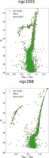 |
Fig. A.1 : Comparison of our cluster membership with literature. Two GCs are compared, NGC 3201 and NGC 288. We define Vasiliev & Baumgardt (2021) as VB21; Hunt & Reffert (2023) as Hunt 2023. |
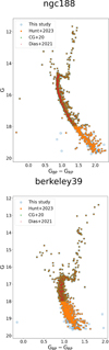 |
Fig. A.2 : Comparison of our cluster membership with literature. Two OCs are compared, NGC188 and Berkeley 39. We define Hunt & Reffert (2023) as Hunt+2023; Cantat-Gaudin et al. (2020) as CG+20 and Dias et al. (2021) as Dias+2021. |
Appendix B Analysis
To obtain astrophysical parameters for BSSs we use three different approaches: i) Color-temperature relations; ii) Model isochrone fitting; iii) Spectroscopic data from Gaia DR3 (if available).
B.1 Color-temperature relations
Based on the infrared flux method (IRFM) from González Hernández & Bonifacio (2009), the effective temperature of a star can be estimated using the following relation.
![Mathematical equation: $\theta=b_{0}+b_{1} C+b_{2} C^{2}+b_{3}[\mathrm{Fe} / \mathrm{H}]+b_{4}[\mathrm{Fe} / \mathrm{H}]^{2}+b_{5}[\mathrm{Fe} / \mathrm{H}] C$](/articles/aa/full_html/2025/07/aa52195-24/aa52195-24-eq160.png) (B.1)
(B.1)
where θ=5040 K / Teff, C is the dereddened color and [Fe/H] is the metallicity. We use the coefficients bi=0 – 5 from Mucciarelli et al. (2021), which are based on a Gaia EDR3 analysis of dwarf and giant stars. [Fe/H] are taken from Carretta et al. (2009) and Dias et al. (2021) for GCs and OCs, respectively. For Pismis 3 and Trumpler 23, metallicities were taken from Bisht et al. (2022) and Overbeek et al. (2017), respectively.
B.2 Isochrone-fitting models
Previous studies have attempted to extract BSS parameters based on isochrone models such as JS21 and D23. In the first study, the authors assumed that the mass of the BSSs to be approximately the mass of a point at the ZAMS with the same magnitude. In the second study, they fit multiple isochrones with different ages and compare BSS positions with respect to the isochrones. We take an approach similar to the second one. For GCs (OCs), we use multiple PARSEC isochrones (Bressan et al. 2012) from 200 Myr (100 Myr) in steps of 50 Myr (25 Myr) up to the cluster age found with the best-isochrone fitting, fixing the metallicity from the literature for each cluster as described earlier. We select the three closest points on the best-fit isochrone for each cluster and compute the average and rms for mass, luminosity, age, surface gravity and effective temperature for each BSS.
B.3 Spectroscopy from Gaia DR3
Gaia DR3 includes optical low-resolution spectra for over 220 million stars. As a brief summary, these spectra are measured with two instruments. One covers the blue-optical range (380–680 nm, measured with the “Blue Photometer” instrument) called BP and another covers the infrared range (640 – 1050 nm, measured with the “Red Photometer”) called RP (De Angeli et al. 2023; Montegriffo et al. 2023). These BP/RP spectra, hereafter referred to as XP spectra, have a spectral resolution R ≃ 50− 160 with parameters inferred from “classical” models (Andrae et al. 2023, and references therein), which are highly sensitive to errors in low-resolution spectra, which is the case for Gaia DR3 XP spectra. In another approach, Zhang et al. (2023), based on parameters obtained from higher-resolution spectra (R ≃ 1800) from other surveys, cross-matched them with Gaia DR3 spectra and created a machine-learning model that has the advantage of: i) obtaining astrophysical parameters from higher-resolution spectra, comparing them with the XP spectra and adjust those parameters at lower spectral resolution; ii) being able to find various systematic errors that could not easily be noticed in the XP spectra alone. For this reason, we extract XP parameters (hereafter called XPP) from Zhang et al. (2023) for all our sample BSSs, if available, such as effective temperature and surface gravity. We cross-match the provided parameters with our selected BSSs using Gaia Source ID unique identifier. Finally, Zhang et al. (2023) provides a quality_flag parameter which, in short, is a number to quantify the reliability of the obtained parameters from spectra. The authors suggest a “basic reliability cut” to be at least quality_flag < 8 (note, a lower number indicates more reliable parameters). We decided to only use stars with quality_flag ≤ 4 to ensure we extract only reliable results. More details for these parameters are provided in Section 4 of Zhang et al. (2023).
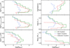 |
Fig. B.1 Histogram of derived astrophysical parameters for our sample BSSs. Top, middle and bottom left panels are the distributions for effective temperatures derived from color-temperature relations, isochrone fittings, and the XPP method (from Gaia DR3 spectroscopy, if available), respectively. Top, middle and bottom right panels are the distributions obtained from isochrone fitting, for BSS ages, luminosities and masses, respectively. GCs are denoted as a red dotted-dashed line, OCs as a dashed blue line and the distribution for all clusters (GCs + OCs) is depicted as a solid green line. |
From the IRFM we find ⟨Teff, IRFM⟩=(6772 ± 630) K for GCs and ⟨Teff, IRFM⟩=(7598 ± 1476) K for OCs. From isochrone fitting we find ⟨Teff, isochrone⟩=(6829 ± 529) K for GCs and ⟨Teff, isochrone⟩=(7549 ± 1331) K for OCs. Only 537 of 4399 BSSs (∼12% of our sample) had XPP parameters measured for 279 stars in GCs and 258 stars in OCs. With this method, we find the mean BSS effective temperature of ⟨Teff, XPP⟩=(7271 ± 732) K for GCs and ⟨Teff, XPP⟩=(7269 ± 1331) K for OCs. Figure B.1 shows the distribution for Teff, L, and M of all our sample BSSs. We also estimated the parameters for YSSs and RSSs, which are available at the CDS. Their distributions are shown in Figure C.1 and Figure C.2 respectively.
To check the consistency of our results, we compare the Teff values obtained from the three methods in Figure B.2 against each other. The top figure is divided into two sub-panels, both of which are comparing Teff derived with the isochrone fitting method against the values found with the IRFM (top-upper panel) and XPP (top-lower panel). The lower panel compares the values of latter two methods against each other. We only consider BSSs with an error in Teff of less than ± 300 K in both components. The 1– to −1 relation is shown as a gray dashed line and is compared with the data. We observe very good agreement between the methods, albeit with small level of systematics. We fit a linear model using LMFIT Python package6 to these relations considering full error propagation in all values, which are shown as a dot-dashed green lines. We also estimated pearson r-coefficients for all these relations in a monte carlo approach, and the estimated values are  (top panel),
  (middle panel) and
  (bottom panel). The errors correspond to 16th and 84th percentile values with respect to the median value. The r-coefficients suggest that estimated Teff from different methods are strongly correlated. We obtain the following linear relations in Kelvin units:
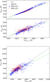 |
Fig. B.2 Top: Teff obtained with isochrone best-fitting method (from PARSEC isochrones, Bressan et al. 2012) compared against Teff obtained via IRFM (color-temperature relations, González Hernández & Bonifacio 2009, upper panel) and XPP (Zhang et al. 2023, lower panel). Bottom: Teff obtained with XPP vs. Teff obtained with IRFM. The 1 -to- 1 relation is shown as a gray dashed line, whereas the best fit (considering GC and OC stars) is shown as a dot-dashed green line. BSSs from GCs are displayed as red stars and BSSs from OCs as blue squares. The figure only displays BSSs whose error in both components is less than 300 K. |
 (B.2)
(B.2)
 (B.3)
(B.3)
 (B.4)
(B.4)
From these results, we note that the Teff extracted from isochrone fitting and those derived from the color-temperature relations (IRFM) appear most consistent with each other up to ∼8000 K, with little systematic offset towards higher IRFM temperature. A similar behavior is observed for the XPP versus isochrone method, where Teff values are consistent within the scatter up to ∼8000 K. Above that temperature, a small systematic offset towards lower XPP temperatures is observed. The bottom panel of Figure B.2 shows the XPP versus IRFM method comparison, which shows the largest scatter yet fairly consistent values for most BSSs, while the linear fit is pulled from 1− to −1 relation by some OC BSSs with temperatures above ∼7500 K.
From these comparisons, we estimate that the systematic uncertainty between various methods is of the order Δ Teff ≃ 100 K. The IRFM and isochrone methods consider the metallicity of the cluster, while the XPP method is inferior for the reasons described in Section B.3, which is reflected in the lower scatter and smaller systematic offset in the IRFM versus isochrone method comparison (upper panel in Fig. B.2). In addition, XPP parameters are not available for stars at the MSTO and therefore we are not able to extract Teff,MSTO using XPP. We therefore consider the IRFM and isochrone method from now as the bona fide best Teff estimates, keeping in mind the systematics described above.
Appendix C Astrophysical parameters for YSSs and RSSs
Similarly to Figure B.1, we display the extracted astrophysical parameters for stars classified as Yellow Straggler Stars (YSSs) and Red Straggler Stars (RSSs) in Figures C.1 and C.2, respectively.
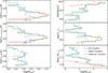 |
Fig. C.1 Same as Figure B.1, but for YSSs. |
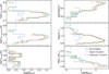 |
Fig. C.2 Same as Figure B.1, but for RSSs. |
Appendix D Parameters of star clusters studied in this paper and the properties of BSSs detected in those clusters
Parameters of star clusters are presented here.
List of BSSs detected in this study and their properties.
References
- Andrae, R., Fouesneau, M., Sordo, R., et al. 2023, A&A, 674, A27 [CrossRef] [EDP Sciences] [Google Scholar]
- Astropy Collaboration (Robitaille, T. P., et al.,) 2013, A&A, 558, A33 [NASA ADS] [CrossRef] [EDP Sciences] [Google Scholar]
- Baldwin, A. T., Watkins, L. L., van der Marel, R. P., et al. 2016, ApJ, 827, 12 [NASA ADS] [CrossRef] [Google Scholar]
- Baumgardt, H., & Vasiliev, E., 2021, MNRAS, 505, 5957 [NASA ADS] [CrossRef] [Google Scholar]
- Baumgardt, H., Hénault-Brunet, V., Dickson, N., & Sollima, A., 2023, MNRAS, 521, 3991 [CrossRef] [Google Scholar]
- Beccari, G., Ferraro, F. R., Dalessandro, E., et al. 2019, ApJ, 876, 87 [NASA ADS] [CrossRef] [Google Scholar]
- Bisht, D., Zhu, Q., Elsanhoury, W. H., et al. 2022, AJ, 164, 171 [Google Scholar]
- Bressan, A., Marigo, P., Girardi, L., et al. 2012, MNRAS, 427, 127 [NASA ADS] [CrossRef] [Google Scholar]
- Burbidge, E. M., & Sandage, A., 1958, ApJ, 128, 174 [Google Scholar]
- Cadelano, M., Ferraro, F. R., Dalessandro, E., et al. 2022, ApJ, 941, 69 [CrossRef] [Google Scholar]
- Cantat-Gaudin, T., Jordi, C., Vallenari, A., et al. 2018, A&A, 618, A93 [NASA ADS] [CrossRef] [EDP Sciences] [Google Scholar]
- Cantat-Gaudin, T., Anders, F., Castro-Ginard, A., et al. 2020, A&A, 640, A1 [NASA ADS] [CrossRef] [EDP Sciences] [Google Scholar]
- Cardelli, J. A., Clayton, G. C., & Mathis, J. S., 1989, ApJ, 345, 245 [Google Scholar]
- Carretta, E., Bragaglia, A., Gratton, R., D’Orazi, V., & Lucatello, S., 2009, A&A, 508, 695 [NASA ADS] [CrossRef] [EDP Sciences] [Google Scholar]
- Chen, X., & Han, Z., 2009, MNRAS, 395, 1822 [Google Scholar]
- Clarkson, W. I., Sahu, K. C., Anderson, J., et al. 2011, ApJ, 735, 37 [NASA ADS] [CrossRef] [Google Scholar]
- Cohen, J., 1988, Statistical Power Analysis for the Behavioral Sciences, 2nd edn. (Hillsdale, NJ: Routledge) [Google Scholar]
- Contreras Ramos, R., Ferraro, F. R., Dalessandro, E., Lanzoni, B., & Rood, R. T., 2012, ApJ, 748, 91 [NASA ADS] [CrossRef] [Google Scholar]
- Cordoni, G., Milone, A. P., Marino, A. F., et al. 2018, ApJ, 869, 139 [CrossRef] [Google Scholar]
- Cordoni, G., Milone, A. P., Mastrobuono-Battisti, A., et al. 2020, ApJ, 889, 18 [Google Scholar]
- Cordoni, G., Milone, A. P., Marino, A. F., et al. 2023, A&A, 672, A29 [NASA ADS] [CrossRef] [EDP Sciences] [Google Scholar]
- Culpan, R., Pelisoli, I., & Geier, S., 2021, A&A, 654, A107 [NASA ADS] [CrossRef] [EDP Sciences] [Google Scholar]
- Curran, P. A., 2014, arXiv e-prints [arXiv:1411.3816] [Google Scholar]
- Da Costa, G. S., 1984, ApJ, 285, 483 [CrossRef] [Google Scholar]
- Dalessandro, E., Ferraro, F. R., Massari, D., et al. 2013, ApJ, 778, 135 [NASA ADS] [CrossRef] [Google Scholar]
- Dattatrey, A. K., Yadav, R. K. S., Rani, S., et al. 2023, ApJ, 943, 130 [CrossRef] [Google Scholar]
- De Angeli, F., Weiler, M., Montegriffo, P., et al. 2023, A&A, 674, A2 [NASA ADS] [CrossRef] [EDP Sciences] [Google Scholar]
- De Marco, O., Shara, M. M., Zurek, D., et al. 2005, ApJ, 632, 894 [NASA ADS] [CrossRef] [Google Scholar]
- Dias, W. S., Monteiro, H., Caetano, T. C., et al. 2014, A&A, 564, A79 [NASA ADS] [CrossRef] [EDP Sciences] [Google Scholar]
- Dias, W. S., Monteiro, H., Moitinho, A., et al. 2021, MNRAS, 504, 356 [NASA ADS] [CrossRef] [Google Scholar]
- Evans, D. W., Riello, M., De Angeli, F., et al. 2018, A&A, 616, A4 [NASA ADS] [CrossRef] [EDP Sciences] [Google Scholar]
- Ferraro, F. R., Paltrinieri, B., Fusi Pecci, F., et al. 1997, A&A, 324, 915 [NASA ADS] [Google Scholar]
- Ferraro, F. R., Beccari, G., Dalessandro, E., et al. 2009, Nature, 462, 1028 [NASA ADS] [CrossRef] [Google Scholar]
- Ferraro, F. R., Lanzoni, B., Dalessandro, E., et al. 2012, Nature, 492, 393 [Google Scholar]
- Ferraro, F. R., Lanzoni, B., Raso, S., et al. 2018, ApJ, 860, 36 [NASA ADS] [CrossRef] [Google Scholar]
- Ferraro, F. R., Lanzoni, B., Vesperini, E., et al. 2023, ApJ, 950, 145 [NASA ADS] [CrossRef] [Google Scholar]
- Fiorentino, G., Lanzoni, B., Dalessandro, E., et al. 2014, ApJ, 783, 34 [NASA ADS] [CrossRef] [Google Scholar]
- Gaia Collaboration (Prusti, T., et al.,) 2016, A&A, 595, A1 [NASA ADS] [CrossRef] [EDP Sciences] [Google Scholar]
- Gaia Collaboration (Brown, A. G. A., et al.,) 2018, A&A, 616, A1 [NASA ADS] [CrossRef] [EDP Sciences] [Google Scholar]
- Gaia Collaboration (Vallenari, A., et al.,) 2023, A&A, 674, A1 [NASA ADS] [CrossRef] [EDP Sciences] [Google Scholar]
- González Hernández, J. I., & Bonifacio, P., 2009, A&A, 497, 497 [Google Scholar]
- Gosnell, N. M., Mathieu, R. D., Geller, A. M., et al. 2015, ApJ, 814, 163 [Google Scholar]
- Harris, W. E., 2010, arXiv e-prints [arXiv:1012.3224] [Google Scholar]
- Hills, J. G., & Day, C. A., 1976, Astrophys. Lett., 17, 87 [NASA ADS] [Google Scholar]
- Hunt, E. L., & Reffert, S., 2023, A&A, 673, A114 [NASA ADS] [CrossRef] [EDP Sciences] [Google Scholar]
- Hurley, J. R., Tout, C. A., & Pols, O. R., 2002, MNRAS, 329, 897 [Google Scholar]
- Iben, I.Jr., 2013, Stellar Evolution Physics, Volume 2: Advanced Evolution of Single Stars (Cambridge, UK: Cambridge University Press) [Google Scholar]
- Jadhav, V. V., & Subramaniam, A., 2021, MNRAS, 507, 1699 [NASA ADS] [CrossRef] [Google Scholar]
- Jadhav, V. V., Sindhu, N., & Subramaniam, A., 2019, ApJ, 886, 13 [NASA ADS] [CrossRef] [Google Scholar]
- Jiang, D., 2022, ApJ, 940, 97 [Google Scholar]
- Jofré, P., Jorissen, A., Van Eck, S., et al. 2016, A&A, 595, A60 [Google Scholar]
- Knigge, C., Leigh, N., & Sills, A., 2009, Nature, 457, 288 [NASA ADS] [CrossRef] [Google Scholar]
- Leigh, N., Sills, A., & Knigge, C., 2011, MNRAS, 416, 1410 [NASA ADS] [CrossRef] [Google Scholar]
- Leiner, E. M., & Geller, A., 2021, ApJ, 908, 229 [Google Scholar]
- Li, C., Zhong, J., Qin, S., & Chen, L., 2023, A&A, 672, A81 [NASA ADS] [CrossRef] [EDP Sciences] [Google Scholar]
- Lombardi, James C., J., Warren, J. S., Rasio, F. A., Sills, A., & Warren, A. R. 2002, ApJ, 568, 939 [NASA ADS] [CrossRef] [Google Scholar]
- Mapelli, M., Sigurdsson, S., Ferraro, F. R., et al. 2006, MNRAS, 373, 361 [Google Scholar]
- Mapelli, M., Ripamonti, E., Battaglia, G., et al. 2009, MNRAS, 396, 1771 [NASA ADS] [CrossRef] [Google Scholar]
- Marigo, P., Girardi, L., Bressan, A., et al. 2008, A&A, 482, 883 [NASA ADS] [CrossRef] [EDP Sciences] [Google Scholar]
- Mathys, G., 1987, A&AS, 71, 201 [NASA ADS] [Google Scholar]
- McCrea, W. H., 1964, MNRAS, 128, 147 [Google Scholar]
- Montegriffo, P., De Angeli, F., Andrae, R., et al. 2023, A&A, 674, A3 [NASA ADS] [CrossRef] [EDP Sciences] [Google Scholar]
- Monteiro, H., Dias, W. S., Moitinho, A., et al. 2020, MNRAS, 499, 1874 [NASA ADS] [CrossRef] [Google Scholar]
- Mucciarelli, A., Bellazzini, M., & Massari, D., 2021, A&A, 653, A90 [NASA ADS] [CrossRef] [EDP Sciences] [Google Scholar]
- Naoz, S., & Fabrycky, D. C., 2014, ApJ, 793, 137 [Google Scholar]
- Nardiello, D., Libralato, M., Piotto, G., et al. 2018, MNRAS, 481, 3382 [NASA ADS] [CrossRef] [Google Scholar]
- Overbeek, J. C., Friel, E. D., Donati, P., et al. 2017, A&A, 598, A68 [NASA ADS] [CrossRef] [EDP Sciences] [Google Scholar]
- Pandey, S., Subramaniam, A., & Jadhav, V. V., 2021, MNRAS, 507, 2373 [NASA ADS] [CrossRef] [Google Scholar]
- Perets, H. B., & Fabrycky, D. C., 2009, ApJ, 697, 1048 [Google Scholar]
- Piotto, G., Milone, A. P., Bedin, L. R., et al. 2015, AJ, 149, 91 [Google Scholar]
- Preston, G. W., & Sneden, C., 2000, AJ, 120, 1014 [Google Scholar]
- Privon, G. C., Ricci, C., Aalto, S., et al. 2020, ApJ, 893, 149 [NASA ADS] [CrossRef] [Google Scholar]
- Rain, M. J., Ahumada, J. A., & Carraro, G., 2021, A&A, 650, A67 [NASA ADS] [CrossRef] [EDP Sciences] [Google Scholar]
- Rao, K. K., Vaidya, K., Agarwal, M., & Bhattacharya, S., 2021, MNRAS, 508, 4919 [Google Scholar]
- Rao, K. K., Bhattacharya, S., Vaidya, K., & Agarwal, M., 2023a, MNRAS, 518, L7 [Google Scholar]
- Rao, K. K., Vaidya, K., Agarwal, M., Balan, S., & Bhattacharya, S., 2023b, MNRAS, 526, 1057 [Google Scholar]
- Raso, S., Ferraro, F. R., Dalessandro, E., et al. 2017, ApJ, 839, 64 [NASA ADS] [CrossRef] [Google Scholar]
- Rodrigo, C., & Solano, E., 2020, in XIV. 0 Scientific Meeting (virtual) of the Spanish Astronomical Society, 182 [Google Scholar]
- Rodrigo, C., Solano, E., & Bayo, A., 2012, SVO Filter Profile Service Version 1.0, IVOA Working Draft 15 October 2012 [CrossRef] [Google Scholar]
- Sandage, A. R., 1953, AJ, 58, 61 [Google Scholar]
- Schultz, G. V., & Wiemer, W., 1975, A&A, 43, 133 [NASA ADS] [Google Scholar]
- Shao, Y., & Li, X.-D. 2016, ApJ, 833, 108 [NASA ADS] [CrossRef] [Google Scholar]
- Shara, M. M., Saffer, R. A., & Livio, M., 1997, ApJ, 489, L59 [NASA ADS] [CrossRef] [Google Scholar]
- Sills, A., Karakas, A., & Lattanzio, J., 2009, ApJ, 692, 1411 [NASA ADS] [CrossRef] [Google Scholar]
- Simunovic, M., 2017, PhD thesis, Ruprecht-Karls University of Heidelberg, Germany [Google Scholar]
- Simunovic, M., & Puzia, T. H., 2016, MNRAS, 462, 3401 [Google Scholar]
- Simunovic, M., Puzia, T. H., & Sills, A., 2014, ApJ, 795, L10 [NASA ADS] [CrossRef] [Google Scholar]
- Sindhu, N., Subramaniam, A., Jadhav, V. V., et al. 2019, ApJ, 882, 43 [NASA ADS] [CrossRef] [Google Scholar]
- Stępień, K., & Kiraga, M., 2015, A&A, 577, A117 [NASA ADS] [CrossRef] [EDP Sciences] [Google Scholar]
- Subramaniam, A., Sindhu, N., Tandon, S. N., et al. 2016, ApJ, 833, L27 [CrossRef] [Google Scholar]
- Vaidya, K., Panthi, A., Agarwal, M., et al. 2022, MNRAS, 511, 2274 [NASA ADS] [CrossRef] [Google Scholar]
- Vasiliev, E., & Baumgardt, H., 2021, MNRAS, 505, 5978 [NASA ADS] [CrossRef] [Google Scholar]
- Virtanen, P., Gommers, R., Oliphant, T. E., et al. 2020, Nat. Methods, 17, 261 [Google Scholar]
- Wasserstein, R. L., & Lazar, N. A., 2016, Am. Statist., 70, 129 [Google Scholar]
- Zhang, X., Green, G. M., & Rix, H.-W., 2023, MNRAS, 524, 1855 [NASA ADS] [CrossRef] [Google Scholar]
Hubble Space Telescope.
Pearson’s test measures whether a pair of two variables are linearly correlated or not. The r-coefficient is defined as the covariance of the variables divided by the product of their standard deviations, and the value ranges from −1 to +1.+1 signifies perfect positive linear correlation between the variables, −1 signifies perfect linear anti-correlation, and 0 means no linear correlation. Based on Cohen (1988), coefficient values >0.5 (< −0.5) indicate a strong positive (negative) linear relation, values between 0.3 and 0.5 (−0.3 and −0.5) indicate a moderate positive (negative) linear relation, and values between 0 and 0.3 (0 and −0.3) indicate a weak positive (negative) linear relation. The Pearson’s test also provides a p-value that indicates whether the observed correlation is statistically significant or not. It depends on the number of data points or the sample size. A smaller p-value (generally <0.05) suggests that the correlation is statistically significant, while for larger values (≥ 0.05), we cannot conclude a significant correlation (Wasserstein & Lazar 2016).
The numbers in all cases denote the correlation coefficient 50th percentile. The lower and upper errors denote the 16th and 75th percentiles, respectively.
Do not confuse this with the BSS double sequences in a CMD discussed earlier, as the upper panel Figure 9 is not a CMD.
All Tables
Comparison between BSS astrophysical parameters obtained in this study against those found in the literature.
All Figures
|
Fig. 1 Histogram for the identified member stars in our sample GCs and OCs (see Sect. 2.1 for details). The distribution for GCs is shown as a dash-dotted red line, for OCs as a dashed blue line, and for the composite sample (GCs+OCs) as a solid green line. The dotted vertical red line with arrows pointing to the right denotes the minimum number of member stars for GCs, and the dotted vertical blue line with arrows pointing to the left indicates the maximum number of identified member stars in OCs. |
| In the text | |
|
Fig. 2 Top: CMD of the GC NGC 6205 using Gaia DR3. Stars that were discarded as cluster members using our selection procedure are shown as gray dots, while cluster members are plotted as black dots. The blue shaded area represents our selection area for BSSs, YSSs and RSSs (see Sect. 2.2) which are shown as blue, yellow and red dots, respectively. The magenta solid curve represents the best-fitting PARSEC isochrone, with the + symbol indicating the MSTO. The right panels show the VPDs for the stars in the respective magnitude range from the left panel. Green crosses represent the median of confirmed members for both components in the VPD. Bottom: same as the top figure, but for the OC NGC 188. We added a red border in the selection area for OCs to avoid AGB/RGB stars (see text for details). |
| In the text | |
|
Fig. 3 Top panel: absolute number of BSSs vs. age of parent cluster found in this work and other Gaia-based studies. Uncertainties in the BSS number are assumed as Poisson errors. The inset sub-panel shows a zoom-in on the GC age range for better visualization. The dashed black line denotes the “ridge-line” based on the sliding histogram (see text for details). Bottom panel: ratio of BSS numbers relative to the number of MS stars in the luminosity range between MSTO and MSTO+1 mag (see Sect. 3.1). We compare the ratio against those studies that also provide this parameter with the same criteria for MS stars number selection, if available. From the considered studies (see legend), only R21 and Cordoni et al. (2023) have this parameter available. Data based in our work is plotted only for those GCs whose NMS is not cut by the photometric depth selection described in Section 2.1; this is done to guarantee a consistent comparison between different clusters and samples. For the uncertainty in NBSS/NMS we assume a simple error propagation with Poisson errors for MS stars and BSSs. Errors in age for GCs are based on the difference between our best-fitting isochrone models and those derived from Baumgardt et al. (2023), whereas errors in ages for OCs are taken from Dias et al. (2021). Similar to the top figure, the black-dashed line represents the “ridge-line” based on the sliding histogram. |
| In the text | |
|
Fig. 4 Teff vs. cluster age. Top: ⟨ Teff⟩ – the mean of the difference between BSS Teff and MSTO Teff, found with the same method, for stars within the same cluster – vs. cluster age. Blue triangles and red dots represent Teff obtained from color-temperature relations for OCs and GCs, respectively. Green plus symbols (+) and orange squares represent Teff derived from isochrone models for OCs and GCs, respectively. At the top right corner we show the results only for GCs without error bars for a better appreciation, keeping the same axes from the major plot. Error bars along vertical axis show the dispersion of BSSs Teff. Middle: difference between ⟨ Teff⟩ and the MSTO Teff, normalized by the MSTO temperature. Horizontal gray dashed line indicates BSS Teff=1.5 × MSTO Teff. Bottom: dispersion of BSS Teff vs. cluster age. |
| In the text | |
|
Fig. 5 Mass of BSSs. Left: mass of BSSs (found with isochrone models) vs. parent cluster age. Upper panel shows the mass of the BSSs, the middle panel shows the difference between the BSS mass and the MSTO mass, and the lower panel shows the mass excess factor, |
| In the text | |
|
Fig. 6
|
| In the text | |
|
Fig. 7 Comparison for |
| In the text | |
|
Fig. 8 Gaia photometry color-magnitude diagram for BSSs classified by their |
| In the text | |
|
Fig. 9 Top: |
| In the text | |
|
Fig. 10 log(AgeBSS) and |
| In the text | |
|
Fig. 11 CMD for BSSs classified as “upper” and “lower” sequences, based on sequences shown Figure 9, for GC NGC362 and OC Berkeley 39. ZAMS and ZAMS – 0.75 mags are displayed as a purple dashed line and as a green dash-dotted line, respectively. Orange plus (+ symbol) and magenta line represent the MSTO and the best-fitting PARSEC isochrone, respectively (similar to Figure 2). Field/non-member stars are displayed as gray points, whereas confirmed members are displayed as black points. BSSs that lie in the upper-sequence and lower-sequence are symbolized as orange squares and red dots, respectively. |
| In the text | |
|
Fig. A.1 : Comparison of our cluster membership with literature. Two GCs are compared, NGC 3201 and NGC 288. We define Vasiliev & Baumgardt (2021) as VB21; Hunt & Reffert (2023) as Hunt 2023. |
| In the text | |
|
Fig. A.2 : Comparison of our cluster membership with literature. Two OCs are compared, NGC188 and Berkeley 39. We define Hunt & Reffert (2023) as Hunt+2023; Cantat-Gaudin et al. (2020) as CG+20 and Dias et al. (2021) as Dias+2021. |
| In the text | |
|
Fig. B.1 Histogram of derived astrophysical parameters for our sample BSSs. Top, middle and bottom left panels are the distributions for effective temperatures derived from color-temperature relations, isochrone fittings, and the XPP method (from Gaia DR3 spectroscopy, if available), respectively. Top, middle and bottom right panels are the distributions obtained from isochrone fitting, for BSS ages, luminosities and masses, respectively. GCs are denoted as a red dotted-dashed line, OCs as a dashed blue line and the distribution for all clusters (GCs + OCs) is depicted as a solid green line. |
| In the text | |
|
Fig. B.2 Top: Teff obtained with isochrone best-fitting method (from PARSEC isochrones, Bressan et al. 2012) compared against Teff obtained via IRFM (color-temperature relations, González Hernández & Bonifacio 2009, upper panel) and XPP (Zhang et al. 2023, lower panel). Bottom: Teff obtained with XPP vs. Teff obtained with IRFM. The 1 -to- 1 relation is shown as a gray dashed line, whereas the best fit (considering GC and OC stars) is shown as a dot-dashed green line. BSSs from GCs are displayed as red stars and BSSs from OCs as blue squares. The figure only displays BSSs whose error in both components is less than 300 K. |
| In the text | |
|
Fig. C.1 Same as Figure B.1, but for YSSs. |
| In the text | |
|
Fig. C.2 Same as Figure B.1, but for RSSs. |
| In the text | |
Current usage metrics show cumulative count of Article Views (full-text article views including HTML views, PDF and ePub downloads, according to the available data) and Abstracts Views on Vision4Press platform.
Data correspond to usage on the plateform after 2015. The current usage metrics is available 48-96 hours after online publication and is updated daily on week days.
Initial download of the metrics may take a while.