| Issue |
A&A
Volume 685, May 2024
|
|
|---|---|---|
| Article Number | A33 | |
| Number of page(s) | 15 | |
| Section | Galactic structure, stellar clusters and populations | |
| DOI | https://doi.org/10.1051/0004-6361/202347499 | |
| Published online | 01 May 2024 | |
Binary origin of blue straggler stars in Galactic star clusters
1
European Southern Observatory, Alonso de Córdova 3107, Vitacura, Región Metropolitana, Chile
e-mail: This email address is being protected from spambots. You need JavaScript enabled to view it.
2
Instituto de Astrofísica de La Plata, IALP (CONICET-UNLP), 1900 La Plata, Argentina
3
Instituto de Física de Rosario, IFIR (CONICET-UNR), 2000 Rosario, Argentina
4
Facultad de Ciencias Exactas, Ingeniería y Agrimensura (UNR), 2000 Rosario, Argentina
5
Facultad de Ciencias Astronómicas y Geofísicas, Universidad Nacional de La Plata (UNLP), La Plata, Argentina
6
Dipartimento di Fisica e Astronomia, Università di Padova, Vicolo Osservatorio 3, 35122 Padova, Italy
7
Departamento de Astronomía, Universidad de Concepción, 160 Casilla, Concepción, Chile
Received:
18
July
2023
Accepted:
2
February
2024
Abstract
Building on the recent release of a new Gaia-based blue straggler star catalog in Galactic open star clusters (OCs), we explored the properties of these stars in a cluster sample spanning a wide range in fundamental parameters. We employed Gaia EDR3 to assess the membership of any individual blue or yellow straggler to their parent cluster. We then made use of the ASteCA code to estimate the fundamental parameters of the selected clusters, in particular, the binary fraction. With all this at hand, we critically revisited the relation of the blue straggler population and the latter. For the first time, we found a correlation between the number of blue stragglers and the host cluster binary fraction and binaries. This supports the hypothesis that binary evolution is the most viable scenario of straggler formation in Galactic star clusters. The distribution of blue stragglers in the Gaia color-magnitude diagram was then compared with a suite of composite evolutionary sequences derived from binary evolutionary models that were run by exploring a range of binary parameters: age, mass ratio, period, and so forth. The excellent comparison between the bulk distribution of blue stragglers and the composite evolutionary sequences loci further supports the binary origin of most stragglers in OCs and paves the way for a detailed study of individual blue stragglers.
Key words: binaries: general / blue stragglers / open clusters and associations: general
© The Authors 2024
 Open Access article, published by EDP Sciences, under the terms of the Creative Commons Attribution License (https://creativecommons.org/licenses/by/4.0), which permits unrestricted use, distribution, and reproduction in any medium, provided the original work is properly cited.
This article is published in open access under the Subscribe to Open model. This email address is being protected from spambots. You need JavaScript enabled to view it. to support open access publication.
1. Introduction
Defying the traditional single stellar evolution with their position in the optical color-magnitude diagram (CMD), they are bluer and brighter than the main-sequence turn-off (MS-TO) of the system in which they are found, blue straggler stars (BSSs) and recently, yellow straggler stars (YSSs, which may be evolved BSSs) are exotic objects that have fascinated theorists and observers equally for generations. While BSSs were initially discovered in globular clusters (GCs; Piotto et al. 2004; Salinas et al. 2012), they are now known to exist in open clusters (OCs; Ahumada & Lapasset 2007; Rain et al. 2021a), dwarf galaxies (Momany et al. 2007), and even in the field of the Milky Way (e.g., Santucci et al. 2015). Since their detection on the core of globular cluster M3 (Sandage 1953), many formation mechanisms have been proposed. Most of them agree that a main sequence (MS) star has gained mass either through mass transfer (MT) from an evolving primary star via Roche-lobe overflow (RLOF; McCrea 1964) and/or via collisions involving single, binary, or even triple stars (Hills & Day 1976). The two basic scenarios can be modified by the presence of a third or additional star. Perets & Fabrycky (2009) proposed a scenario in which the inner binary in a hierarchical triple system can coalesce due to perturbations of the outer companion, producing in the end a BSS in a binary system with a long period.
With the advent of the second Gaia data release, a renaissance of the study of BSSs on individuals and across a large sample of OCs took recently place (Bhattacharya et al. 2019; Rain et al. 2020, 2021b,a; Rani et al. 2023; Vaidya et al. 2020; Jadhav & Subramaniam 2021; Leiner & Geller 2021; Rao et al. 2023). It is possible today to accurately identify genuine BSSs candidates while distinguishing them from outliers and field stars by combining Gaia parallax measurements, proper motions, and star colors to establish membership with a high degree of certainty. In this study, we use Gaia EDR3 to select members of a sample of 12 old (> 9.0 Gyr), relatively nearby (d < 5000 parsecs), rich OCs, with the goal of understanding the BS population and their connection with binaries in the host cluster.
The data on BSSs and YSSs allow us to perform a detailed comparison with theoretical predictions. For this purpose, we present detailed calculations of binary evolution to explore whether the hypothesis of a binary origin holds. The quantities necessary to define a particular binary are the stellar masses, the orbital period of the pair, and the type of mass transfer, conservative or nonconservative. Thus, performing a full exploration of the parameter space of the problem represents a major numerical effort that may be warranted in a future study. We restrict ourselves here to a given (fixed) initial mass ratio and conservative MT.
The layout of this study is as follows: we first describe our selection of the sample and the cluster members in Sect. 2, and in Sect. 3, we define the regions whithin which the blue and yellow straggler candidates where selected. In Sect. 4 we describe the estimation of fundamental parameters. Then, in Sect. 5, we search for correlations between the cluster parameters and the straggler population. In Sect. 6 we introduce binary evolution models, and in Sect. 7 we compare them with the blue straggler star distribution in the color-magnitude diagram. In Sect. 8 we provide our summary and conclusions.
2. Selection of the cluster sample and members
The clusters were first selected on the basis of the number of blue stragglers. Only those with NBSS ≥ 8 listed in the most recently published catalog of BSSs in OCs (Rain et al. 2021a) were selected. The original list contained a total of 32 clusters with log(age)≥9.0 dex (1 Gyr, Dias et al. 2021), distances d > 850 pc (Cantat-Gaudin & Anders 2020), and masses M > 1400 M⊙ (Jadhav & Subramaniam 2021).
For the 32 clusters, we performed a membership selection using the Gaia astrometric solution. The cluster members were estimated via a two-step process. First, we downloaded the data of each cluster by using a simple script to query EDR3 data using the Astroquery package1. This package generates two user-defined colors (not present in the raw Gaia data) with their associated uncertainties. This is currently not provided in Gaia. The last was useful for the process described in Sect. 4 (Sect. 4). For each cluster, we then selected all the stars within twice the apparent radius reported in Dias et al. (2002) and with magnitudes down to Gmag = 18.5. Second, the most likely members for each cluster were identified with the pyUPMASK code (Pera et al. 2021). This tool assigns probability membership Pmemb values to all the stars in an observed frame based on input data selected by the user. In this case, we employed parallax and proper motion data that we downloaded from the Gaia EDR3 survey as the input data.
After assigning probabilities, the final member list was automatically generated by an iterative process. This process works by filtering out low-probability stars at each step and halts when the density of stars within the cluster region is consistent with the expected density, taking into account the field density value outside the adopted cluster region. After this membership analysis, we removed nine clusters from our list because of their sparse nature. With only a handful of subgiant (SGB) and read giant branch (RGB) stars, these clusters have large errors for the few observed stars and can lead to an overestimation of the parameters (e.g., mass and age), and therefore, we did not consider them reliable enough for the main aim of this work.
In particular, the Gaia photometric bands are broad enough to introduce large color differences caused by extinction as a function of the stellar SED. These spreads in color can introduce dispersion in the CMD positions, affecting the selection, especially near the TO. As shown by Leiner & Geller (2021), for clusters with low reddening values (E(GBP − GRP) < 0.3), it is sufficient to adopt the reddening from the literature and convert it into the Gaia passbands. On the other hand, for clusters with higher values of E(GBP − GRP), individual (star by star) reddening corrections are recommended.
In Rain et al. (2021b) we determined the reddening law RG = AG/E(GBP − GRP) by a linear least-squares fit and obtained RG = 1.79 ± 0.05. This value was adopted as the slope of the reddening law for all the clusters. Here, we carried out the reddening corrections using MS stars. For these, we defined a line along the MS, and for each one of the selected MS stars, we calculated its distance from this line to the reddening law line. The vertical projection of this distance gives the differential AG absorption at the position of the star, while the horizontal projection gives the differential reddening E(GBP − GRP) at the stellar position. After this first step, we selected for each star of the field (both cluster members and nonmembers) the ten nearest MS stars and calculated the mean differential AG absorption and the mean differential E(GBP − GRP), and we finally subtracted this mean value from its (GBP − GRP) color and G magnitude. Although they are sufficiently rich, seven clusters situated beyond 5.5 Kpc and with an extinction between 1.0 < Av < 2.5 exhibit a considerable variation in the color of their MS and giant branches, particularly in the TO region. As a result, it becomes very challenging to accurately fit isochrones and define the blue (and yellow) region, as explained in Sect. 3.
3. Blue and yellow straggler regions
Although a great variety of definitions is available in the literature (Ahumada & Lapasset 2007; Bhattacharya et al. 2019; Rain et al. 2020; Vaidya et al. 2020, and references therein) to define the blue straggler region, we closely followed the most recent definitions using Gaia data (Leiner & Geller 2021; Rain et al. 2021a). The procedure we used is the following: (i) After the membership selection (see Sect. 2), the photometric data were plotted in the G versus (GBP − GRP) diagram. (ii) An approximate matching of a MIST theoretical isochrone (Dotter 2016) with the Gaia EDR3 passbands and assuming the parameters of each cluster calculated by Dias et al. (2021) was then performed on the main sequence and TO, and eventually on the RGB and red clump (RC), if present. (iii) Then, we identified the bluest point in the best-fit isochrone. We used the blue hook when available, and otherwise, the TO to set this limit. Only objects significantly detached from this point, for instance, ∼0.03 mag as a minimum and down to 0.5 mag at most below the TO, were listed as blue straggler candidates. (iv) We plotted the equal-mass binary sequence obtained by displacing the isochrone by 0.75 mag upward, which represents the maximum brightness expected for an equal-mass binary at the cluster TO location. The very same sequence was helpful to identify the yellow straggler stars and also to set the lower limit (on brightness) of this population. Stars brighter than this sequence but redder than the blue stragglers and bluer than the red giant branch falling into this region were considered yellow straggler candidates (see Fig. 1). Gaia CMDs of the remaining clusters are shown in Appendix A. After this step, only clusters with NBSS ≥ 9 remained in our list. Four clusters were left out because they had a relatively low number of stragglers.
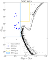 |
Fig. 1. Color-magnitude diagram of the open cluster NGC 6819 to illustrate the selection of BSSs and YSSs. The light blue and yellow lines separate the different regions in which we searched for these stars. The MIST isochrone is shown for comparison. |
4. Estimation of the fundamental parameters with ASteCA
The fundamental parameters for all the clusters (age, binary fraction, distance, metallicity, extinction, and mass) were estimated with the ASteCA package (Perren et al. 2015). This package has been used to successfully analyze hundreds of clusters since its release (Perren et al. 2017, 2020). To simplify the Bayesian inference, the process that estimates the fundamental parameters, we assumed a general solar metallicity and allowed the rest of the parameters to vary within reasonable ranges. The estimation of the binary fraction depends on the chosen distribution of primary to secondary masses q = m1/m2 (mass ratio), where m1 is the primary mass of a binary system, and m2 is the secondary mass. Here, the distribution is specified to be uniform as
 (1)
(1)
with qmax = 1.43. The shape of these distributions approximates the empirical distributions found in works such as Fisher et al. (2005) and Raghavan et al. (2010), where the mass ratio is close to unity (m2 ≈ m1) and drops rapidly for lower values (m2 ≤ 0.51m1). The results for each cluster are reported in Table 1. At this point. it is important to mention that opting for a uniform distribution would lead to a higher binary fraction value because of the increased production of binary systems with lower secondary masses. Hence, it is appropriate to view our binary fraction value as a conservative lower limit.
Parameters of open clusters in our sample adopted for this study.
5. Searching for correlations
An alternative way of obtaining insight into the relative efficiency of the formation mechanisms of BSSs is to investigate possible correlations between the blue straggler population and the host cluster properties. We therefore compared the observed number of BSSs (NBSS) with the physical parameters of the 12 OCs of the sample. In particular, we searched for possible correlations between the raw number of BSSs (NBSS), the binary fraction (fbin), and the number of binaries Nbin of each cluster. Furthermore, to statistically measure the strength of the relation between the variables, we used the Spearman rank correlation test. The coefficient (rs) and confidence levels (p-value) for the considered parameter pairs are reported in Figs. 2 and 3.
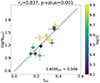 |
Fig. 2. Logarithm of the observed number of blue straggler stars a function of the binary fraction. The dashed black line indicates the best fit to the data. The color bar indicates the age of each cluster. Errors are Poissonian. |
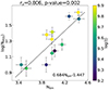 |
Fig. 3. Logarithm of the observed number of BSSs as a function of the number of binaries on each cluster. The dashed black line indicates the best fit to the data. The errors are Poissonian. |
We revisited the correlation between NBSS and cluster binary fraction. Open clusters are both less massive and younger than globular clusters. Their proximity and low density make the determination of the binary frequency particularly easy. Furthermore, in open clusters, the relation between this parameter and straggler numbers has never been explored in detail before. We find a dependence  and a Spearman coefficient value of rs = 0.83. This correlation is shown in Fig. 2 with the corresponding line of the best fit to the data. As in the case of the GCs, here, the relation is continuous (Milone et al. 2012) and can be considered as the continuation of that found between core binary fraction and straggler numbers in low-density clusters by Sollima et al. (2008).
Within the same context, the cluster mass inside the core radius has been considered by different authors to be the best indicator of blue straggler population size in stellar clusters (e.g., Knigge et al. 2009; Leigh et al. 2011). We found a dependence of  on δ = 0.6 ± 0.2 here. These values are higher than the predicted value reported on Knigge et al. (2009) (
 ) for GCs, but they agree with the recent upper limit found for OCs
  (Jadhav & Subramaniam 2021).
According to Leigh et al. (2013), when most of the BSSs are descended from binary evolution, a dependence of the form
 (2)
(2)
is expected, where  is the average stellar mass, which the authors assumed to be the same for every cluster. We assumed this to be 0.4 M⊙.
In comparison with the binary fraction, the correlation with the Nbin decreases. When using Eq. (2), the Spearman rank coefficient rs decreased in ∼0.03. This means that the correlation becomes weaker by adding MTot (see Fig. 3). This behavior was predicted by Knigge et al. (2009) and previously tested by Leigh et al. (2013) in GCs. Our results agree with their findings, that is, the strength of the correlation (NBSS vs. Mcore) decreases when fbin is included. Within our sample, we found a dependence of the form  .
.
Finally, and differently from the previous cases, no correlation at all was found between the specific frequency ( )2 and Mcore or Nbin. The absence of a correlation between these parameters is expected, however, because according to Knigge et al. (2009), Eq. (2) only holds for the blue straggler numbers and not for the specific frequency.
6. Binary evolution and the formation of blue straggler stars
To theoretically account for the observed properties of BSSs, we performed a set of detailed binary evolution calculations. The results presented below represent our first attempt to reproduce them.
When considering binary evolution calculations, a set of quantities has to be defined (the initial masses of the stars and the orbital period; the type of mass transfer, see below, and the chemical composition, etc.). Thus, performing a full exploration of the parameter space represents a major numerical effort.
For the calculations presented in this paper, we employed an updated version of the code for stellar binary evolution described in Benvenuto & De Vito (2003). Briefly, this code solves the structure of spherical stars assuming they move along a circular orbit. It allows the computation of conservative and nonconservative mass transfer episodes. When the pair is detached, it works as a standard Henyey code. Conversely, hen the donor has a size comparable to that of its Roche lobe and a mass transfer sets in (a semidetached pair), it computes the structure of the donor, the orbital evolution, and the mass transfer rate simultaneously.
The calculations were performed assuming that there is no mass loss from the system: All the material transferred by the donor is accreted by its companion. This process causes the system to become a blue straggler and eventually, a yellow straggler. Conservation of mass represents an extreme case of binary evolution in which the BSSs phenomenon is strongest. Evidently, if the companions were able to retain only a fraction of the transferred mass, the increase in mass and luminosity would be smaller.
In order to compute the evolution of a binary system, we first considered the evolution of the donor star. By doing this, we determined the structure of this star, the mass transfer rate, the chemical composition of the material lost by the donor, and the orbital evolution. After this, with the mass transfer rate (Ṁ) from the previous calculation, we performed the detailed evolution of the companion star (the accretor). As a result of accretion and internal evolution, this star filled its own Roche lobe in most cases. At this moment, the components of the system were in contact, and we stopped the calculations. The object that emerged from contact is expected to be one of those observed in any case.
We tuned the mixing length parameter to reproduce the present Sun, considered moderate overshooting, semiconvection as in Langer et al. (1983), and thermohaline mixing following Maeder et al. (2013). The chemical evolution of the models was solved as in Langer et al. (1985) considering noninstantaneous mixing. We neglected effects of stellar rotation in these calculations.
We assumed solar composition stars. The donor masses ranged from 0.82 M⊙ to 1.60 M⊙ with a step of 25%; for the accretor, we simply assumed an initial mass ratio of 1.25, and the initial orbital period interval extended from 0.26 d to 1.95 d, again with a step of 25% (see Table 2).
Binary models.
The choice of the initial mass ratio of 1.25 was made to perform the first step of our exploration of the BSSs phenomenon. We designed these calculations with the aim of quantitatively testing the correctness of the hypotheses we developed to explain BSSs in open clusters. A more exhaustive exploration of possible configurations with other initial mass ratios will be the subject of future investigations.
Stellar evolution calculations provide the bolometric luminosity and effective temperature of each star of the pair, among other quantities. However, observations do not detect the donor and the accretor separately, but together as one object. To allow a direct comparison of models with data, after solving for the evolution of each star of the pair, we therefore added their contributions to compute its evolution in the theoretical CMD (see below Sect. 6.2). These results are to be compared with observations.
6.1. Evolutionary results
Figure 4 shows an example of our results. We show the evolution of a pair of 1.28 M⊙ + 1.02 M⊙ on an orbit with an initial period of one day. The system evolves on a detached configuration up to an age of ≈4.9 Gyr, when the donor star fills its Roche lobe. At this moment, it has already exhausted its hydrogen core. It accordingly undergoes class B mass transfer. From then on, the star follows a completely different evolution from that of an isolated star of the same mass and composition. Prior to RLOF, the companion star evolves very slowly, but when it begins to accrete mass, it becomes brighter on a very short (thermal) timescale. The evolution was followed up to an age of 5.89 Gyr when the accretor also fills its Roche lobe and the system is in contact.
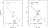 |
Fig. 4. Evolution of a pair of 1.28 M⊙ + 1.02 M⊙ on an orbit with an initial period of one day. The filled points are labeled with their corresponding ages. The open circles denote the occurrence of the RLOF at an age of ≈4.9 Gyr. At this moment, it has already exhausted its hydrogen core. Left panel: evolution of the components of the pair in the theoretical plane of bolometric luminosity vs. effective temperature. Right panel: each track in the CMD and also the track to be observed by a remote observer that cannot resolve the pair. |
In the left panel of Fig. 4, we depict the evolution of the system in the typical theoretical plane, and in the right panel, we show each of the tracks in the CMD (see Sect. 6.2 below). In this panel, we also include the track to be observed by a remote observer that cannot resolve the pair. We call this sequence a composite evolutionary sequence.
In Table 2 we list the computed binaries, where we indicate with MA and MB the masses of donor and accretor stars in solar mass units, respectively, and the initial orbital period in days.
In closing this section, a comparison of our work with approaches and results presented by other authors is in order. Tian et al. (2006) studied the formation of BSSs by mass transfer in close binary systems in a somewhat similar way to the way adopted in this paper. Employing the Eggleton code (Han et al. 2000) and assuming conservative mass transfer, they computed a set of binary systems for a variety of donor and accretor masses and orbital separations. They applied this set to perform a population study for the conditions of the old OC NGC 2682 (M67), concluding that at least for the case this OC, other mechanisms must operate that lead to BSSs formation in addition to mass transfer in binaries. Among other more recent works, we cite those of Sun et al. (2021) and Sun & Mathieu (2023). In each of these papers, the authors presented a study of a particular BSS (WOCS 5379 and WOCS 4540, both located in the OC NGC 188) based on detailed models constructed with the MESA code (Paxton et al. 2011), searching for the models that best account for their main characteristics. They allowed for the possibility of nonconservative mass transfer. Another study, presented by Leiner & Geller (2021), considered a population analysis of BSSs based on simulations performed with the rapid code presented by Hurley et al. (2002), which allows approximately computing a large number of systems. Binary stellar evolution strongly depends on more parameters (masses, orbital period, the type of mass transfer, and chemical composition) than isolated objects, but also on the stability of the mass transfer process transfer. The results presented by Leiner & Geller (2021) strongly depend on some approximations that strongly affect the output of the calculations, in particular, the critical mass ratio for stable mass transfer qcrit.
We compared our effort with those presented in the four papers specifically devoted to BSSs that we cited above. In this paper, we do not try to fit models to a particular BSS as in Sun et al. (2021) or Sun & Mathieu (2023), but search for a wider view of the problem. While our models are detailed, they are unable to provide a picture of the problem as wide as that given by the population analysis of Leiner & Geller (2021). The approach assumed by Tian et al. (2006) is more similar to ours, although there are some remarkable differences. They computed a family of detailed evolutionary tracks under similar assumptions regarding the mass transfer process (conservation of mass and angular momentum) for a variety of masses and initial periods and employed them in a population study for NGC 2682. We worked with a fixed pair-mass, however, which allowed a variety of initial periods, and we applied it to a variety of clusters, but did not simulate any population synthesis.
The detailed comparison of our models with those presented in the above-cited works is an important and not easy task. In order to avoid deviating from the main objective of this paper, we defer this analysis to a future publication.
6.2. Colors and magnitudes in the Gaia system
For all our binaries, we computed Gaia EDR3 filters to perform color-magnitude diagrams. To this end, we solved the atmosphere structure of our models in local thermodynamic equilibrium. The code we used is an updated version of the code described in Rohrmann (2001). It takes into account hydrostatic and radiative-convective equilibrium. When the star model had a cold atmosphere, convective transport was treated with the mixing-length approximation.
We computed the atmosphere models separately for each pair of binaries, that is, we obtained two sequences in the color-magnitude diagram for each binary. The emergent magnitude results from the sum of both fluxes, resulting in the composite evolutionary sequence. First, we computed the filter-weighted integrated fluxes Fi for each model,
 (3)
(3)
where i = A, B. The letter A represents the donor star, and the letter B denotes the accretor star, f(λ) is the computed absolute flux, and RX(λ) is the response function of filter X. In Eq. (3), the integration is over the filter bandpass X in wavelength (angstroms), and the integrated flux FX, i is used to calculate magnitudes in each band by means of
 (4)
(4)
where MX, i and CX are the synthetic magnitude and the flux constant for the X band, respectively. The flux constant is defined such that the synthetic magnitude matches the Vega magnitude in X band. However, when we observe the combined flux, then we should consider the following:
![Mathematical equation: $$ \begin{aligned} \nonumber \frac{\int [ f_A(\lambda ) + f_B(\lambda ) ] R_X(\lambda ) \mathrm{d}\lambda }{\int R_X(\lambda ) \mathrm{d}\lambda }=F_{X,A} + F_{X,B}. \end{aligned} $$](/articles/aa/full_html/2024/05/aa47499-23/aa47499-23-eq12.gif)
Using Eq. (4), we obtain
 (5)
(5)
When the binary system is not eclipsing,
 (6)
(6)
hence,
![Mathematical equation: $$ \begin{aligned} M_{X,A+B}=-2.5 \log (10^{0.4 C_X} [10^{-0.4 M_{X,A}}+10^{-0.4 M_{X,B}}]) + C_X. \end{aligned} $$](/articles/aa/full_html/2024/05/aa47499-23/aa47499-23-eq15.gif) (7)
(7)
The sequences we show below were computed using the transformation given in Eq. (7) for the binary models listed in Table 2.
In Fig. 5, we depict the transformed binary sequences.
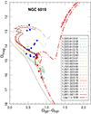 |
Fig. 5. Color-magnitude diagram for NGC 6819. We depict the combined binary tracks as solid, dotted, short-dashed, long-dashed, and three short-dashed colored lines. The dotted black line depicts the ZAMS, and the dot-dashed red line denotes the isochrone for NGC 6819 (in Log(t[yr])) for single models. The filled blue circles indicate BSSs, and the filled red circles indicate the age on tracks. The three numbers in the box denote the M1/M2/P donor mass (in M⊙), the accretor mass (in M⊙), and the period (in days). |
7. Cluster-by-cluster discussion
In this section, we comment on the comparison between binary star models and the distribution of stragglers in the Gaia color-magnitude diagrams. Before entering the cluster-by-cluster analysis, we stress that the comparison is qualitative at this stage because we lack crucial information about basic straggler properties such as mass and period. The obvious aim of this comparison is to highlight that binary evolution models can fit the general distribution of BSSs in the cluster CMDs well.
7.1. NGC 6819
The comparison is illustrated in Fig. 5. The distribution of bona fide BSS members (filled blue circles) is compared with evolutionary tracks for the mass ratios indicated in the inset. For reference, the cluster best-fit isochrone is drawn with dashed-dotted line. This cluster harbors BSSs with very different luminosity, and they seem to form two groups. A bright group of three BSSs comes from the binary evolution of pairs with high-mass donors (1.28 M⊙), while the fainter group follows the evolutionary path of pairs with lower-mass donors (1.02 M⊙). Overall, the binary tracks match the BSS distribution excellently. Some BSSs are in the stage of leaving their MS according to the models.
7.2. Berkeley 32
In this old open cluster, most BSSs are crowded immediately above the TO. However, a number of BSSs is much brighter than the TO, and they cover a large range in magnitude (up to 5 magnitudes; see Figs. A.1a and B.1a). The cluster hosts two YSSs as well. The large excursion in magnitude (and hence in mass) implies that very different binary evolution tracks have to be employed to cover the BSS region. We note that both BSSs and YSSs are well fit by these models, however. Finally, a few faint stragglers are not reproduced by the suite of models we ran. These faint stars may be misclassified stragglers. Another possibility is that different parameters of the binary model need to be adopted.
7.3. Berkeley 39
The location of BSS candidates in the CMD of this cluster is shown in Figs. A.1b and B.1b. As noted for other cases (see below), the BSS candidates are separated into two main groups. One group consists of faint BSSs that closely follow the low-mass donor tracks. The other group contains BSSs that are spread in color and is significantly redder than the ZAMS. These are well matched by the binary star evolutionary models with a donor mass in the range 1.28 − 1.60 M⊙ overimposed in the CMD. Berkeley 39 also contains two YSSs. As in the case of Berkeley 32 and given our stringent and conservative selection criteria, some of these stars can be misclassifications and/or it could be necessary to consider different parameters for the binary model.
7.4. Collinder 261
This cluster harbors a rich population of BSS candidates. They compose a continuous luminosity sequence that overlaps either with the ZAMS or with binary evolution sequences. We note that several BSSs lie below and redward of the cluster TO. If these two BSSs are confirmed, they might be two examples of the so-called sub-subdwarfs (Geller et al. 2017b,a). Another interesting case is the bright BSS immediately above the cluster TO, which looks like a promising YSS candidate, but fails to follow the standard criterion for the location of these stars in the CMD. The very faint BSS candidate at G ∼ 17.2 might be a misidentification, or might more conservatively be off the ZAMS because of larger photometric errors. CMDs of Collinder 261 can be found in Figs. A.1c and B.1c.
7.5. Melotte 66
The BSSs for this cluster seem to form a double sequence (see Figs. A.1d and B.1d). A first sequence follows a low-mass donor (∼1.02 M⊙) tracks and is relatively close to the cluster ZAMS. A second redder sequence is also tightly aligned with the binary tracks. It has a pair with a 1.28 M⊙ donor. Double sequences have widely been discussed in GCs, and many authors claimed that they can be used as tracers of a core-collapse event and subsequent dynamical evolutionary phases in GCs. NGC 6256 (Cadelano et al. 2022), NGC362 (Dalessandro et al. 2013), and NGC 1261 (Simunovic et al. 2014) are notable examples for which authors have explored these double sequences. The red BSS sequence is interpreted as populated by MT products (Xin & Deng 2015), and the blue narrow sequence may be reproduced by collisions or merger products (Sills et al. 2009). This is not universal, however, as W UMa contact binaries were discovered in the blue and red sequence of the GC M30 Ferraro et al. (2009). A few studies (e.g., Stȩpień & Kiraga 2015; Jiang et al. 2017) indicated that a binary evolution contributes to the formation of blue stragglers in both sequences. As in our case, Rao et al. (2023) found that this feature is present in OCs. These authors claimed, more conservatively, that MT causes the formation of both sequences. Furthermore, Rao et al. (2022) performed a multiwavelength spectral energy distribution (SED) fitting for 12 out of the 18 BSSs of Melotte 66, and only 2 of them (BSS3, Gaia DR3 5507234395259864448, and BSS6, 5507234429619602944) were identified as MT products. All the remaining stragglers are consistent with a single-component SED. Interestingly enough, the two binary stars fall within the blue sequence. Unfortunately, given the lack of studies, no other variable stars have been reported within the Melotte 66 blue straggler population. Additional spectroscopic observations or light-curve modeling is required to confirm the binary nature of the remaining 16 BSSs and to constrain its spectroscopic parameters, rotational velocity, mass, and so on. An analysis of the individual nature of blue stragglers and the origin of the apparent double sequences in Melotte 66 is far beyond the scope of this paper, however. Additionally, we confirm that single YSS candidate (yellow dot) is interpreted as an evolved binary system.
7.6. NGC 188
Like M 67 (see below), this cluster has been studied very extensively, and its population of BSSs is quite well established. Their distribution is shown in Figs. A.2a and B.2a. The BSS region is crossed by several binary star evolutionary tracks, which confirm the interpretation that BBS candidates far from the ZAMS are the result of some type of binary star evolution.
7.7. NGC 2141
This rich cluster hosts a significant number of BSS candidates (see Figs. A.2b and B.2b). We cannot exclude that some of them are a misidentification, in particular, those very close to the cluster sequence and TO. In any case, the bulk of these BBS is well matched by the binary evolution tracks for the masses indicated in the inset. Moreover, the YSS (yellow dot) is quite well reproduced.
7.8. NGC 2158
The distribution of BSS candidates is shown in Figs. A.2c and B.2c. A significant number of BSS candidates lies blueward of the ZAMS. This might be a misidentification or the product of photometric errors. We conservatively considered them to be single BSSs that follow the cluster ZAMS. The distribution of all the other BSS candidates is well reproduced by the set of binary star evolutionary models, including the one yellow straggler.
7.9. NGC 2243
This old open cluster (Figs. A.2d and B.2d) has only a few BSSs. As seen in other cases, the BSS candidates that do not lie along the ZAMS (five to six, in this case) are well matched by binary evolution tracks. Some of them (two to three) also appear to be evolved binary systems, but they are not yet in the so-called YSS region according to the standard definition.
7.10. NGC 2506
This cluster is illustrated in Fig. A.3a. With the exception of just one BSS that lies at the top of the ZAMS, all the candidate BSSs follow the pattern of binary star evolution covering a sizeable luminosity range. The BSSs are not very numerous, as in the case of NGC 2682 (see below), but this clearly depends on the cluster mass. No YSSs are detected.
7.11. NGC 2682
The population of BSSs in M67 was frequently studied in the past. Several of these stars have indeed been identified as binaries. This is confirmed by the overall agreement between BSS candidates and the binary tracks in Figs. B.3b. The cluster also harbors two YSSs that seem to be evolved binary systems (see Fig. B.3b).
7.12. NGC 7789
NGC 7789, like Melotte 66, is a rich and compact old open cluster. Although less evident than in Melotte 66, a double sequence of BSSs seems to be present in NGC 7789 as well (see Figs. A.3c and B.3d). The two sequences are almost parallel, one follows low-mass donor (1.28 M⊙) tracks, the other follows the MS of the binary tracks with parameters 1.60, 1.28, and 1.25. Additionally, employing a time-series radial velocity analysis, the study by Nine et al. (2020) revealed binary characteristics of four BSSs. Moreover, in a separate work, Vaidya et al. (2022) presented the SED of five BSS candidates, confirming the presence of a hot companion for all five. Two of these stars overlap with the sample identified by Nine et al. (2020). The remaining eight BSSs did not exhibit any type of variability. Upon comparing their findings with our own, we observed that all BSSs, regardless of whether they are binary or single, exhibit a random distribution in the CMD.
8. Summary
The aim of this work was twofold. On the one hand, we focused on estimating the binary fraction in a sample of BSSs hosting old open clusters to assess the relation between the population of BSSs and the parent cluster binary fraction. On the other hand, we compared the distribution of BSSs in the cluster CMD with the evolutionary track of binary star evolution at varying mass ratio.
Using the Python unsupervised algorithm pyUPMASK and the automated stellar cluster analysis (ASteCA) package, we identified cluster members, cluster parameters, and blue straggler populations. We estimated the binary fraction, mass, distance, and age for a total of 12 open clusters, and we investigated their possible relation with the observed number of BSSs, NBSS. Finally, we compared the distribution of the straggler population in the color-magnitude diagram with a set of evolutionary tracks derived from binary evolution models.
Our research provided direct evidence that clusters within our regime produce BSSs more efficiently. Furthermore, we confirmed that the number of BSSs is influenced by the binary fraction (fbin), mass, and the number of binaries (Nbin), and that the correlation with the binary fraction is the strongest predictor of the blue straggler population size with a Spearman coefficient of rs ∼ 0.84, followed by the number of binaries and the total mass, with rs = 0.80 and rs = 0.58, respectively. Additionally, as in the case of the GCs, we found that the correlation between the stragglers and Nbin improves the previously known sublinear correlation between the straggler numbers and the mass of the cluster.
We also estimated the dependence of the straggler size and the different cluster parameters. We found a dependence of the form (in decreasing order)  ,
,  , and
, and  for the number of binaries, the total cluster mass, and the binary fraction, respectively.
On the other hand, having established these observational pieces of evidence, we employed evolutionary models of binary star evolution to explore the multidimensional parameter of the mass ratio, primary mass, and period. Lacking precise estimates of the BSS period, the exploration at this stage was rather qualitative. We still showed that for all the clusters under investigation, the binary evolution tracks can reproduce the bulk of the BSSs distribution in the CMDs well. One of the most interesting outcomes is the evidence of a dichotomy in the BSSs distribution in a few clusters. We identified a sequence of stragglers lying close to the cluster ZAMS, while the other sequence follows the binary evolution tracks better. This is similar to the BSSs distribution that was recently found in some globular clusters. We cannot argue, however, that this is a general feature because we do not see it clearly in all clusters, possibly because of photometric errors or an uncertain membership. We are confident that with more precise observational data, in particular, with the knowledge of the binary period, a better comparison can be performed in the future and that the properties of several stragglers can be revealed. An additional improvement is certainly to search for a more precise binary mass ratio for each of these clusters. Our assumed mass ratio of 0.7 does not produce a perfect fit for all the clusters we studied.
With pleasure, we thank the anonymous referee for the many valuable suggestions and comments, which improved the paper greatly.
 .
.
Acknowledgments
The work of M.J. Rain and G. Carraro has been supported by Padova University grant BIRD191235/19: Internal dynamics of Galactic star clusters in the Gaia era: binaries, blue stragglers, and their effect in estimating dynamical masses. O. G. Benvenuto is member of the Carrera del Investigador Científico, Comisión de Investigaciones Científicas de la Provincia de Buenos Aires, Argentina. S. Villanova gratefully acknowledges the support provided by Fondecyt regular n. 1220264 and by the ANID BASAL projects FB210003.
References
- Ahumada, J. A., & Lapasset, E. 2007, A&A, 463, 789 [NASA ADS] [CrossRef] [EDP Sciences] [Google Scholar]
- Benvenuto, O. G., & De Vito, M. A. 2003, MNRAS, 342, 50 [NASA ADS] [CrossRef] [Google Scholar]
- Bhattacharya, S., Vaidya, K., Chen, W. P., & Beccari, G. 2019, A&A, 624, A26 [EDP Sciences] [Google Scholar]
- Cadelano, M., Ferraro, F. R., Dalessandro, E., et al. 2022, ApJ, 941, 69 [CrossRef] [Google Scholar]
- Cantat-Gaudin, T., & Anders, F. 2020, A&A, 633, A99 [NASA ADS] [CrossRef] [EDP Sciences] [Google Scholar]
- Dalessandro, E., Ferraro, F. R., Massari, D., et al. 2013, ApJ, 778, 135 [NASA ADS] [CrossRef] [Google Scholar]
- Dias, W. S., Alessi, B. S., Moitinho, A., & Lépine, J. R. D. 2002, A&A, 389, 871 [NASA ADS] [CrossRef] [EDP Sciences] [Google Scholar]
- Dias, W. S., Monteiro, H., Moitinho, A., et al. 2021, MNRAS, 504, 356 [NASA ADS] [CrossRef] [Google Scholar]
- Dotter, A. 2016, ApJS, 222, 8 [Google Scholar]
- Ferraro, F. R., Beccari, G., Dalessandro, E., et al. 2009, Nature, 462, 1028 [NASA ADS] [CrossRef] [Google Scholar]
- Fisher, J., Schröder, K.-P., & Smith, R. C. 2005, MNRAS, 361, 495 [NASA ADS] [CrossRef] [Google Scholar]
- Geller, A. M., Leiner, E. M., Bellini, A., et al. 2017a, ApJ, 840, 66 [NASA ADS] [CrossRef] [Google Scholar]
- Geller, A. M., Leiner, E. M., Chatterjee, S., et al. 2017b, ApJ, 842, 1 [NASA ADS] [CrossRef] [Google Scholar]
- Han, Z., Tout, C. A., & Eggleton, P. P. 2000, MNRAS, 319, 215 [Google Scholar]
- Hills, J. G., & Day, C. A. 1976, Astrophys. Lett., 17, 87 [NASA ADS] [Google Scholar]
- Hurley, J. R., Tout, C. A., & Pols, O. R. 2002, MNRAS, 329, 897 [Google Scholar]
- Jadhav, V. V., & Subramaniam, A. 2021, MNRAS, 507, 1699 [NASA ADS] [CrossRef] [Google Scholar]
- Jiang, D., Chen, X., Li, L., & Han, Z. 2017, ApJ, 849, 100 [NASA ADS] [CrossRef] [Google Scholar]
- Knigge, C., Leigh, N., & Sills, A. 2009, Nature, 457, 288 [NASA ADS] [CrossRef] [Google Scholar]
- Langer, N., Fricke, K. J., & Sugimoto, D. 1983, A&A, 126, 207 [NASA ADS] [Google Scholar]
- Langer, N., El Eid, M. F., & Fricke, K. J. 1985, A&A, 145, 179 [NASA ADS] [Google Scholar]
- Leigh, N., Sills, A., & Knigge, C. 2011, MNRAS, 416, 1410 [NASA ADS] [CrossRef] [Google Scholar]
- Leigh, N., Knigge, C., Sills, A., et al. 2013, MNRAS, 428, 897 [NASA ADS] [CrossRef] [Google Scholar]
- Leiner, E. M., & Geller, A. 2021, ApJ, 908, 229 [Google Scholar]
- Maeder, A., Meynet, G., Lagarde, N., & Charbonnel, C. 2013, A&A, 553, A1 [NASA ADS] [CrossRef] [EDP Sciences] [Google Scholar]
- McCrea, W. H. 1964, MNRAS, 128, 147 [Google Scholar]
- Milone, A. P., Piotto, G., Bedin, L. R., et al. 2012, A&A, 540, A16 [NASA ADS] [CrossRef] [EDP Sciences] [Google Scholar]
- Momany, Y., Held, E. V., Saviane, I., et al. 2007, A&A, 468, 973 [NASA ADS] [CrossRef] [EDP Sciences] [Google Scholar]
- Nine, A. C., Milliman, K. E., Mathieu, R. D., et al. 2020, AJ, 160, 169 [NASA ADS] [CrossRef] [Google Scholar]
- Paxton, B., Bildsten, L., Dotter, A., et al. 2011, ApJS, 192, 3 [Google Scholar]
- Pera, M. S., Perren, G. I., Moitinho, A., Navone, H. D., & Vazquez, R. A. 2021, A&A, 650, A109 [NASA ADS] [CrossRef] [EDP Sciences] [Google Scholar]
- Perets, H. B., & Fabrycky, D. C. 2009, ApJ, 697, 1048 [Google Scholar]
- Perren, G. I., Vázquez, R. A., & Piatti, A. E. 2015, A&A, 576, A6 [NASA ADS] [CrossRef] [EDP Sciences] [Google Scholar]
- Perren, G. I., Piatti, A. E., & Vázquez, R. A. 2017, A&A, 602, A89 [NASA ADS] [CrossRef] [EDP Sciences] [Google Scholar]
- Perren, G. I., Giorgi, E. E., Moitinho, A., et al. 2020, A&A, 637, A95 [NASA ADS] [CrossRef] [EDP Sciences] [Google Scholar]
- Piotto, G., De Angeli, F., King, I. R., et al. 2004, ApJ, 604, L109 [Google Scholar]
- Raghavan, D., McAlister, H. A., Henry, T. J., et al. 2010, ApJS, 190, 1 [Google Scholar]
- Rain, M. J., Carraro, G., Ahumada, J. A., et al. 2020, AJ, 159, 59 [Google Scholar]
- Rain, M. J., Ahumada, J. A., & Carraro, G. 2021a, A&A, 650, A67 [NASA ADS] [CrossRef] [EDP Sciences] [Google Scholar]
- Rain, M. J., Carraro, G., Ahumada, J. A., et al. 2021b, AJ, 161, 37 [NASA ADS] [CrossRef] [Google Scholar]
- Rani, S., Pandey, G., Subramaniam, A., & Rao, N. K. 2023, ApJ, 945, 11 [NASA ADS] [CrossRef] [Google Scholar]
- Rao, K. K., Vaidya, K., Agarwal, M., et al. 2022, MNRAS, 516, 2444 [NASA ADS] [CrossRef] [Google Scholar]
- Rao, K. K., Bhattacharya, S., Vaidya, K., & Agarwal, M. 2023, MNRAS, 518, L7 [Google Scholar]
- Rohrmann, R. D. 2001, MNRAS, 323, 699 [Google Scholar]
- Salinas, R., Jílková, L., Carraro, G., Catelan, M., & Amigo, P. 2012, MNRAS, 421, 960 [Google Scholar]
- Sandage, A. R. 1953, AJ, 58, 61 [Google Scholar]
- Santucci, R. M., Placco, V. M., Rossi, S., et al. 2015, ApJ, 801, 116 [Google Scholar]
- Sills, A., Karakas, A., & Lattanzio, J. 2009, ApJ, 692, 1411 [NASA ADS] [CrossRef] [Google Scholar]
- Simunovic, M., Puzia, T. H., & Sills, A. 2014, ApJ, 795, L10 [NASA ADS] [CrossRef] [Google Scholar]
- Sollima, A., Lanzoni, B., Beccari, G., Ferraro, F. R., & Fusi Pecci, F. 2008, A&A, 481, 701 [NASA ADS] [CrossRef] [EDP Sciences] [Google Scholar]
- Stȩpień, K., & Kiraga, M. 2015, A&A, 577, A117 [NASA ADS] [CrossRef] [EDP Sciences] [Google Scholar]
- Sun, M., & Mathieu, R. D. 2023, ApJ, 944, 89 [NASA ADS] [CrossRef] [Google Scholar]
- Sun, M., Mathieu, R. D., Leiner, E. M., & Townsend, R. H. D. 2021, ApJ, 908, 7 [NASA ADS] [CrossRef] [Google Scholar]
- Tian, B., Deng, L., Han, Z., & Zhang, X. B. 2006, A&A, 455, 247 [NASA ADS] [CrossRef] [EDP Sciences] [Google Scholar]
- Vaidya, K., Rao, K. K., Agarwal, M., & Bhattacharya, S. 2020, MNRAS, 496, 2402 [Google Scholar]
- Vaidya, K., Panthi, A., Agarwal, M., et al. 2022, MNRAS, 511, 2274 [NASA ADS] [CrossRef] [Google Scholar]
- Xin, Y., & Deng, L. 2015, Astrophys. Space Sci. Libr., 413, 317 [NASA ADS] [CrossRef] [Google Scholar]
Appendix A: Observational color-magnitude diagrams
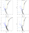 |
Fig. A.1. Color-magnitude diagrams of all 11 remaining clusters in our sample. The filled black circles are the Gaia members selected as described in Sect. 2. The filled blue and yellow circles are the blue and yellow straggler stars selected as described in Sect. 3. The black line shows the corresponding isochrone (Dotter 2016) with the age, Av, and [Fe/H] value of each cluster. |
Appendix B: Theoretical color-magnitude diagrams
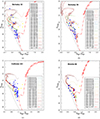 |
Fig. B.1. Color-magnitude diagrams. The combined binary tracks are represented as solid, dotted, short-dashed, long-dashed, and three short-dashed colored lines. The dotted black lines depict the ZAMS, and dot-dashed red lines represent the corresponding isochrones (in Log(t[yr])) for single models. The BSSs are indicated by filled blue circles, and YSSs are shown by filled yellow circles. The filled red circles indicate the cluster age. The sets of three numbers denote the M1/M2/P donor mass (in M⊙), the accretor mass (in M⊙), and the period (in days). |
All Tables
All Figures
|
Fig. 1. Color-magnitude diagram of the open cluster NGC 6819 to illustrate the selection of BSSs and YSSs. The light blue and yellow lines separate the different regions in which we searched for these stars. The MIST isochrone is shown for comparison. |
| In the text | |
|
Fig. 2. Logarithm of the observed number of blue straggler stars a function of the binary fraction. The dashed black line indicates the best fit to the data. The color bar indicates the age of each cluster. Errors are Poissonian. |
| In the text | |
|
Fig. 3. Logarithm of the observed number of BSSs as a function of the number of binaries on each cluster. The dashed black line indicates the best fit to the data. The errors are Poissonian. |
| In the text | |
|
Fig. 4. Evolution of a pair of 1.28 M⊙ + 1.02 M⊙ on an orbit with an initial period of one day. The filled points are labeled with their corresponding ages. The open circles denote the occurrence of the RLOF at an age of ≈4.9 Gyr. At this moment, it has already exhausted its hydrogen core. Left panel: evolution of the components of the pair in the theoretical plane of bolometric luminosity vs. effective temperature. Right panel: each track in the CMD and also the track to be observed by a remote observer that cannot resolve the pair. |
| In the text | |
|
Fig. 5. Color-magnitude diagram for NGC 6819. We depict the combined binary tracks as solid, dotted, short-dashed, long-dashed, and three short-dashed colored lines. The dotted black line depicts the ZAMS, and the dot-dashed red line denotes the isochrone for NGC 6819 (in Log(t[yr])) for single models. The filled blue circles indicate BSSs, and the filled red circles indicate the age on tracks. The three numbers in the box denote the M1/M2/P donor mass (in M⊙), the accretor mass (in M⊙), and the period (in days). |
| In the text | |
|
Fig. A.1. Color-magnitude diagrams of all 11 remaining clusters in our sample. The filled black circles are the Gaia members selected as described in Sect. 2. The filled blue and yellow circles are the blue and yellow straggler stars selected as described in Sect. 3. The black line shows the corresponding isochrone (Dotter 2016) with the age, Av, and [Fe/H] value of each cluster. |
| In the text | |
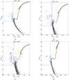 |
Fig. A.2. Same as. Fig. A.1. |
| In the text | |
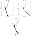 |
Fig. A.3. Same as. Fig. A.1. |
| In the text | |
|
Fig. B.1. Color-magnitude diagrams. The combined binary tracks are represented as solid, dotted, short-dashed, long-dashed, and three short-dashed colored lines. The dotted black lines depict the ZAMS, and dot-dashed red lines represent the corresponding isochrones (in Log(t[yr])) for single models. The BSSs are indicated by filled blue circles, and YSSs are shown by filled yellow circles. The filled red circles indicate the cluster age. The sets of three numbers denote the M1/M2/P donor mass (in M⊙), the accretor mass (in M⊙), and the period (in days). |
| In the text | |
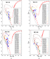 |
Fig. B.2. Same as Fig. B.1. |
| In the text | |
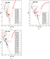 |
Fig. B.3. Same as Fig. B.1. |
| In the text | |
Current usage metrics show cumulative count of Article Views (full-text article views including HTML views, PDF and ePub downloads, according to the available data) and Abstracts Views on Vision4Press platform.
Data correspond to usage on the plateform after 2015. The current usage metrics is available 48-96 hours after online publication and is updated daily on week days.
Initial download of the metrics may take a while.