| Issue |
A&A
Volume 697, May 2025
|
|
|---|---|---|
| Article Number | A72 | |
| Number of page(s) | 19 | |
| Section | Cosmology (including clusters of galaxies) | |
| DOI | https://doi.org/10.1051/0004-6361/202453450 | |
| Published online | 12 May 2025 | |
Deep Chandra observations of PLCKG287.0+32.9: A clear detection of a shock front in a heated former cool core
1
Dipartimento di Fisica e Astronomia (DIFA), Università di Bologna, Via Gobetti 93/2, 40129 Bologna, Italy
2
Istituto Nazionale di Astrofisica (INAF) – Istituto di Radioastronomia (IRA), Via Gobetti 101, I-40129 Bologna, Italy
3
University of California Observatories/Lick Observatory, Dept. of Astronomy and Astrophysics, Santa Cruz, CA 95064, USA
4
INAF – Istituto di Astrofisica Spaziale e Fisica Cosmica di Milano, Via A. Corti 12, 20133 Milano, Italy
5
Center for Astrophysics, Harvard & Smithsonian, 60 Garden Street, Cambridge, MA 02138, USA
6
Leiden Observatory, Leiden University, PO Box 9513 2300 RA Leiden, The Netherlands
7
University of Hamburg, Hamburger Sternwarte, Gojenbergsweg 112, 21029 Hamburg, Germany
⋆ Corresponding author: This email address is being protected from spambots. You need JavaScript enabled to view it.
Received:
14
December
2024
Accepted:
17
March
2025
Abstract
Context. The massive, hot galaxy cluster PSZ2 G286.98+32.90 (hereafter PLCKG287, z = 0.383) hosts a giant radio halo and two prominent radio relics that are signs of a disturbed dynamical state. Gravitational lensing analysis shows a complex cluster core with multiple components. However, despite optical and radio observations indicating a clear multiple merger, the X-ray emission of the cluster, derived from XMM-Newton observations, shows only moderate disturbance.
Aims. The aim of this work is to study the X-ray properties and investigate the core heating of such a massive cluster by searching for surface brightness discontinuities and associated temperature jumps that would indicate the presence of shock waves.
Methods. We present new 200 ks Chandra X-ray Observatory ACIS-I observations of PLCKG287 and perform a detailed analysis to investigate the morphological and thermodynamical properties of the region inside R500 (∼1.5 Mpc).
Results. The global X-ray morphology of the cluster has a comet-like shape, oriented in the NW-SE direction, with an ∼80 kpc offset between the X-ray peak and the brightest cluster galaxy (BCG). We detect a shock front in the NW direction at a distance of ∼390 kpc from the X-ray peak, characterized by a Mach number of ℳ ∼ 1.3, as well as a cold front at a distance of ∼300 kpc from the X-ray peak, nested in the same direction as the shock in a typical configuration expected for a merger. We also find evidence for X-ray depressions to the E and W, which could be the signature of feedback from the active galactic nucleus (AGN). The radial profile of the thermodynamic quantities shows a temperature and abundance peak in the cluster’s center, where the pressure and entropy also exhibit a rapid increase.
Conclusions. Based on these properties, we argue that PLCKG287 is what remains of a cool core after a heating event. We estimate that both the shock energy and the AGN feedback energy, implied by the analysis of the X-ray cavities, are sufficient to heat the core to the observed temperature of ∼17 keV in the central ≈160 kpc. We discuss the possible origin of the detected shock by investigating alternative scenarios of merger and AGN outburst, finding that they are both energetically viable. However, no single model seems able to explain all the X-ray features detected in this system. This suggests that the combined action of merger and central AGN feedback is likely necessary to explain the reheated cool core, the large-scale shock, and the cold front. The synergy of these two processes may act to shape the distribution of cool core and non-cool core clusters.
Key words: radiation mechanisms: non-thermal / methods: observational / galaxies: clusters: general / galaxies: clusters: intracluster medium / galaxies: clusters: individual: PSZ2 G286.98+32.90 / X-rays: galaxies: clusters
© The Authors 2025
 Open Access article, published by EDP Sciences, under the terms of the Creative Commons Attribution License (https://creativecommons.org/licenses/by/4.0), which permits unrestricted use, distribution, and reproduction in any medium, provided the original work is properly cited.
This article is published in open access under the Subscribe to Open model. This email address is being protected from spambots. You need JavaScript enabled to view it. to support open access publication.
1. Introduction
The hierarchical model of structure formation predicts that clusters of galaxies grow by the successive accretion of smaller subunits through mergers (e.g., Kravtsov & Borgani 2012; Vikhlinin et al. 2014, for reviews). A large amount of energy is dissipated in the intra-cluster medium (ICM), and possibly channeled into the amplification of the magnetic fields (e.g., Dolag et al. 2008, for a review) and into the acceleration of high-energy cosmic rays (e.g., Petrosian & Bykov 2008; Brunetti & Jones 2014, for reviews), which in turn may produce observable radio emission. Merger events may also shape the thermodynamical properties of the ICM and thus affect the distribution of cool core and non-cool core clusters. However, theory and simulations studies showcase an ongoing debate on whether mergers are solely responsible for disrupting cool cores, or whether other processes, such as feedback from active galactic nuclei (AGNs), are at play (e.g., McCarthy et al. 2008; Guo & Mathews 2010; Rasia et al. 2015; Barnes et al. 2018). Therefore, detailed observations of disturbed systems are key to investigating this problem (e.g., Molendi et al. 2023).
The cluster PSZ2 G286.98+32.90, also known in the literature as PLCKG287.0+32.9 (hereafter PLCKG287), is a massive cluster with M500 ∼ 13.7 × 10¹⁴ M⊙ (Planck Collaboration XXVII 2016) located at redshift z = 0.383 (D’Addona et al. 2024). It was the second most significant detection of the Planck Sunyaev–Zel’dovic (S–Z) survey (Planck Collaboration, 2010), and a 10 ks validation observation performed with XMM-Newton revealed that it is extremely hot (kT500 ∼ 13 keV) and luminous ( erg s−1) within R500 (∼1.5 Mpc). PLCKG287 belongs to the CHEX-MATE cluster sample (Cluster HEritage project with XMM-Newton: Mass Assembly and Thermodynamics at the Endpoint of structure formation, CHEX-MATE Collaboration 2021). Follow-up XMM-Newton observations have been carried out by the CHEX-MATE collaboration to achieve a robust determination of the thermal properties up to R500, confirming that it is a very luminous and hot cluster (Riva et al. 2024).
The dynamical and thermodynamical properties of the cluster have been analyzed by several authors (Bagchi et al. 2011; Bonafede et al. 2014; Finner et al. 2017, 2024; Campitiello et al. 2022; Golovich et al. 2019; Riva et al. 2024). Bagchi et al. (2011) first analyzed the cluster, concluding that it is undergoing one or multiple mergers with the main axis oriented in the direction from northwest (NW) to southeast (SE). The merger orientation is confirmed by optical ESO 2.2 m WFI data, which indicate that PLCKG287 is located within a 6-Mpc-long intergalactic filament and has undergone a major merger, slightly misaligned with respect to the main direction of accretion (Bonafede et al. 2014). In addition, two more sub-clumps are detected along the filament.
Giant Metrewave Radio Telescope (GMRT) and Karl G. Jansky Very Large Array (JVLA) radio observations from 150 MHz to 3 GHz show that the cluster hosts diffuse radio emission (Bagchi et al. 2011; Bonafede et al. 2014; Stuardi et al. 2022), as is expected for massive merging clusters. In particular, the cluster hosts two symmetrically radio relics, which are supposed to be generated by merger-driven shock fronts, and a radio halo, which is connected to the (re)acceleration of cosmic ray electrons by turbulence (e.g., Brunetti & Jones 2014; van Weeren et al. 2019, and references therein). The radio halo appears to be roundish in shape at 325 MHz, with a total extent of ∼ 250″ (1.3 Mpc), and co-spatial with the cluster X-ray emission. At 150 MHz, the halo is reported to be more elongated toward the SE, reaching a largest angular size of ∼450″, corresponding to ∼2.4 Mpc (Bonafede et al. 2014). The relics are found along the merger axis, as they are usually found in this kind of source. Other peculiar features of filamentary radio emission whose origin is unknown have also been detected (Bonafede et al. 2014).
More recent Subaru optical observations confirm that the galaxy distribution is elongated in the SE to NW direction along the merger axis and that the mass distribution on large scales also follows the same merger axis (Finner et al. 2017, 2024). The higher-resolution Hubble Space Telescope (HST) mass map shows that two mass peaks exist within the central mass clump, and that they also lie along the merger axis. The cluster mass is dominated by the primary cluster of mass M ∼ 1.6 × 10¹⁵ M⊙ centered on the brightest cluster galaxy (BCG), with three substructures that are ∼10% of the mass of the primary cluster. Based on the spatial distribution of the substructures, Finner et al. (2017) conclude that they are consistent a with merger scenario that may have created the radio relics.
Despite optical and radio analysis indicating a clear massive and strong multiple merger, the X-ray emission of the cluster shows moderate disturbance with only a single peak. Indeed, the X-ray morphological analysis of Campitiello et al. (2022) classifies PLCKG287 as having a “mixed morphology”, being ranked 87th out of 118 clusters in the CHEX-MATE sample in terms of morphological disturbance. Hence, PLCKG287 could be a case in which a merger has not completely disrupted the cluster core, as is observed in several systems (e.g., Douglass et al. 2018; Schellenberger et al. 2023; Rossetti & Molendi 2010, and references therein). Yet, the presence of the halo, relics, other thin radio filaments, and the mass distribution reconstructed by weak lensing analysis make the cluster an intriguing case that needs to be studied in more detail.
The aim of this work is to present a detailed analysis of deep Chandra observations of the cluster PLCKG287, in order to study the X-ray morphological and thermodynamical properties of the ICM. We focus our analysis and discussion on the X-ray properties of the cluster, whereas the connection with the radio features will be studied in detail in forthcoming papers based on new observations with MeerKAT L band (Balboni et al., in prep.), uGMRT (Band3 and Band4), and MeerKAT (UHF and S-band) observations (Rajpurohit et al., in prep.).
The paper is organized as follows. In Sect. 2, we present the Chandra observations and the basic steps of the data reduction. In Sect. 3, we present the global properties of the cluster derived from the morphological and spectral analyses inside R500. In particular, we discuss the residual images obtained by subtracting the best-fit β-model (Sect. 3.1) and the radial profiles and 2D spectral maps of the thermodynamic properties (Sect. 3.2). In Sect. 4, we present the detection of a shock and a cold front based on the detailed analysis of the surface brightness and thermodynamic radial profiles. Our interpretation of the observational results is discussed in Sect. 5, in which we first investigate the possibility that PLCKG287 is a former cool core (Sect. 5.1), then compare the energy required to heat the core (Sect. 5.2) to the energy of the shock (Sect. 5.3) and AGN feedback (Sect. 5.4), and finally discuss the possible scenarios for the origin of the shock (Sect. 5.5). We then present our conclusions in Sect. 6. With H0 = 70 km s−1 Mpc−1 and ΩM = 1 − ΩΛ = 0.3, the luminosity distance to PLCKG287 (z = 0.383) is 2063.7 Mpc and 1″ corresponds to 5.23 kpc in the rest frame of the cluster.
2. Chandra observation and data reduction
We analyzed archival Chandra X-ray Observatory observations of the cluster PLCKG287 consisting of five different exposures (ObsID 17165, 17166, 17494, 17495, 18807; see Table 1). Each observation was obtained with the ACIS-I instrument in VFAINT mode. The footprint of the five available ObsIDs of PLCKG287 is shown in Fig. 1 (left panel), where R500 = 1541 kpc (Bagchi et al. 2011) is indicated with a white circle. The cluster emission extends over all four ACIS-I chips of each ObsID; therefore, we reprocessed all 20 chips. Data were downloaded from the Chandra Data Archive1 and were reprocessed with the software package CIAO (version 4.10) and CALDB (version 4.7.3) to apply the latest calibration available at the time of the analysis and to remove bad pixels and flares. We also improved the absolute astrometry identifying the point sources of the longest exposure (ObsID 17494) with the task WAVDETECT and cross-matching them with the optical catalog USNO-A2.02. The other datasets were then registered to the position of the longest one.
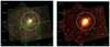 |
Fig. 1. Field of view of the Chandra observations of PLCKG287 (z = 0.383). Left panel: footprint of the five Chandra ObsIDs. Right panel: background-subtracted, exposure-corrected mosaic in the [0.5–7.0] keV band. The detected point sources that were removed from the analysis are shown with green ellipses. In both panels, the white circle indicates R500 = 1541 kpc, which is the region on which we focus our analysis. |
Summary of the Chandra ACIS-I observations analyzed in this work (PI: A. Bonafede).
For the background treatment, we adopted the blank-sky background files3 created by the ACIS calibration team. For each obsID dataset separately, we first identified and re-projected the ACIS blank-sky files that match our data. Then we treated each chip individually, normalizing it to the count rate of the same chip of the corresponding obsID event file in the 9–12 keV band. The background event files thus obtained for each chip were then used for the spectral analysis (Sect. 3.2). Since the blanksky files were created for quiescent-background periods, we additionally filtered our ObsID datasets in the same manner to remove periods of background flares4. The net exposure times obtained after this phase of data cleaning are summarized in Table 1, resulting in a final, combined exposure for the five ObsID datasets of 131.9 ks.
To create a mosaic image, we combined the event files of the five obsID datasets by running merge_obs, which generates an image in units of counts (counts/pixel), an exposure map (cm2 s counts/ photons) and an image in units of flux (photons/(cm2 s pixel)) resulting from the division between the count image and the exposure map. The merge_obs script generates also the PSF map5 of the mosaic used to detect the point sources with WAVDETECT. To create the associated mosaic background image, we proceeded as follows: for each obsID, we created a background event file by combining with dmmerge the reprojected blank-sky files of each chip. This combined blanksky event file was then reprojected to match the corresponding ObsID event file and normalized to the 9-12 keV band count rate of the corresponding ObsID main chip. From the combined blank-sky event file of each ObsID we then created a background image and scaled it to the exposure time of the corresponding obsID. Finally, we combined the five background images with reproject_image. The resulting background-subtracted, exposure-corrected mosaic in the 0.5–7.0 keV band is shown in Fig. 1 (right panel), where the detected point sources (then removed from the analysis) are also shown. Throughout the analysis, error bars are at the 1σ confidence levels on a single parameter of interest, unless otherwise stated.
3. Global cluster properties
3.1. Morphological analysis
In Fig. 2, we show the Chandra image with the superimposition of the GMRT radio contours at 330 MHz from Bonafede et al. (2014). The global X-ray morphology of the cluster has a comet-like shape oriented in the NE-SW direction. The central cluster region encompassed by the radio halo is very bright, with an X-ray peak (located at RA 11:50:49.4, Dec −28:04:44.3) that is offset by 15.2″ (∼80 kpc) from the position of the main BCG (BCG-273, RA 11:50:50.2, Dec −28:04:55.7, D’Addona et al. 2024). This separation, corresponding to roughly 0.05 R500, is indicative of a disturbed dynamical state (e.g., Rossetti et al. 2016). We adopted the X-ray peak as the center of the X-ray analyses presented in this paper.
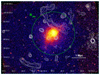 |
Fig. 2. Background-subtracted, exposure-corrected Chandra mosaic of PLCKG287 in the [0.5–7.0] keV band smoothed with a kernel of 4 pixels (1 ACIS pixel = 0.492″). The detected point sources (shown with green ellipses in the right panel of Fig. 1) have been subtracted. The green circle indicates R500 = 1541 kpc. Overlaid in white are the GMRT radio contours at 330 MHz (levels start at ±3σ and increase by a factor of 2, where σ = 0.1 mJy/beam, beam = 12.9″ × 7.9″). The radio data shows two prominent radio relics to the NW and SE at distances of ∼500 kpc and ∼2.8 Mpc kpc from the cluster center. The bright X-ray core region is coincident with a giant radio halo. See Bonafede et al. (2014) for more details on the radio features. |
3.1.1. Surface brightness profile
To study the X-ray morphology of the ICM, we made use of the package pyproffit (Eckert et al. 2020), which is the Python implementation of the proffit C++ software (Eckert et al. 2011) specifically designed for the analysis of galaxy cluster X-ray surface brightness profiles. By providing as input the mosaic count image, background image and exposure map6 (Sect. 2), we extracted the azimuthally averaged surface brightness (SB) profile in 2″-wide annular bins up to R500 (1541 kpc ∼4.9′, indicated by the green circle in Fig. 2). We fit the profile with a single β-model, defined by the function:
 (1)
(1)
where norm is the normalization expressed in units of log10 of the central value, rc is the core radius, and β is the slope parameter. The best-fit (χ2/dof = 217/143 = 1.52) parameters are β = 0.583 ± 0.004 and core radius rc = (0.816 ± 0.013) arcmin ∼(246 ± 1) kpc. We also considered a double β-model, defined by the function
![Mathematical equation: $$ \begin{aligned} \mathrm{SB}(r) = \mathrm{norm} \left[ \left(1 + \left(r/r_{\rm c1} \right)^2 \right)^{0.5 - 3 \beta } + R \, \left(1 + \left(r/r_{\rm c2} \right)^2 \right)^{0.5 - 3 \beta } \right] . \end{aligned} $$](/articles/aa/full_html/2025/05/aa53450-24/aa53450-24-eq3.gif) (2)
(2)
We found that, although it provides a better fit to the central bin (∼10.5 kpc), the F-test indicated that the improvement is not significant (F-stat = 0.66, F-prob = 0.52).
We further extracted the SB profile in elliptical annuli (PA = 33°, axis ratio = 1.5), finding an improvement in the fit (χ2/d.o.f. = 164/143 = 1.15). The best-fit parameter are β = 0.595 ± 0.005 and core radius (measured along the major axis) rc = (1.045 ± 0.018) arcmin ∼(328 ± 6) kpc. On the other hand, we found that restricting the radial range to the central 1.3 arcmin (∼408 kpc), the fits with a single β-model to the SB profiles extracted in circular annuli and elliptical annuli are indistinguishable (χ2/d.o.f. = 31.4/35 and 33.0/35, respectively). We verified that the circular and elliptical fits continue to be consistent at 1σ up to ≈500 kpc. We finally verified that changing the radial binning of the profile extraction by adopting different values and spacing provides consistent best-fit parameters. The results of the fits to the radial profile up to R500 are summarized in Table 2 and the best-fit of the circular and elliptical profile are shown in the left and right panels of Fig. 3, respectively.
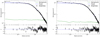 |
Fig. 3. Background-subtracted, azimuthally averaged radial surface brightness profile in the [0.5–7.0] keV energy band extracted in circular (left panel) and elliptical (right panel) annuli. The best-fit to a single β-model is shown with a blue line in both panels. The best-fit parameters are reported in Table 2. The radial distances are in units of arcmin, where 1 arcmin = 313.8 kpc. |
Results of the fit to the surface brightness profile extracted up to R500.
3.1.2. Residual and unsharp images: Analysis of X-ray depressions
The residual image of the central region obtained by subtracting the best-fit elliptical β-model is shown in Fig. 4 (left panel). This image illustrates the deviations of the data from the best-fit β-model. Another method typically used in X-ray imaging to highlight substructures in the ICM is that to produce unsharp masked images. In particular, we smoothed the Chandra image with two Gaussian functions of small (3″–5″) and large (10″–40″) kernel size; then, we derived an unsharp masked image by subtracting the large-scale smoothed image from the small-scale smoothed one. We tried various combinations that image features on different scales, finding generally consistent results. In the right panel of Fig. 4, we show the unsharp image obtained by subtracting the 40″ smoothed image from the 5″ smoothed one. Notable structures such as edges and discontinuities identified in the residual and unsharp images are analyzed and discussed in Sects. 4 and 5.3. We further note a remarkable spatial correspondence between the X-ray feature surrounding the cluster central region (best visible in the unsharp mask image, right panel of Fig. 4) and the outer shape of the giant radio halo. This will be discussed in forthcoming papers (Rajpurohit et al., in prep.; Balboni et al., in prep.).
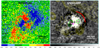 |
Fig. 4. Morphological substructures in PLCKG287 from filtered Chandra images. Left panel: residual Chandra image of the central cluster region obtained by subtracting the best-fit elliptical β-model (see Table 2). As is indicated by the color bar, the positive and negative residuals are shown in red and blue, respectively. Right panel: unsharp masked image obtained by subtracting a 40″-smoothed image from a 5″-smoothed one. The dashed green ellipses show the possible X-ray depressions discussed in Sect. 5.4, whereas the red arc indicates the position of the identified shock front (see Sect. 4). Overlaid are the GMRT radio contours at 330 MHz (same as in Fig. 2). In both panels, the black and magenta crosses indicate the location of the X-ray peak (RA 11:50:49.4, Dec −28:04:44.3) and main BCG (RA 11:50:50.2, Dec −28:04:55.7), respectively. |
The visual inspection of both the residual and unsharp mask images also reveals the presence of possible X-ray depressions in the E-W direction with respect to the center. The analysis of the azimuthal variation in the background-subtracted, exposure-corrected SB around the cluster center, performed in wedges encompassing the X-ray depressions (see Fig. 5, middle panel), indicates that they are significant, particularly the E one (see Fig. 5, left panel). We also investigated the radial variation by extracting the SB profile in four sectors (see Fig. A.1), finding confirmation for a large (size ≈ 80 kpc) depression in the E direction and hints of a smaller (size ≈ 60 kpc) one in the W direction (see Fig. 5, right panel). The interpretation of these features will be discussed in Sects. 5.4 and 5.5.2.
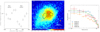 |
Fig. 5. Detection of E-W depressions in PLCKG287. Left panel: azimuthal SB profile around the cluster center extracted along the wedges shown in the middle panel. The largest deficit is in the direction of the E depression seen in the residual and unsharp images (see Fig. 4). A second dip is visible in the azimuthal profile in the direction of the W depression. Angles are measured counterclockwise, with 0° to the West direction, and are shown starting from −90° to improve the visibility of the West deficit in the plot. Middle panel: background-subtracted, exposure-corrected mosaic [0.5–7.0] keV Chandra image, smoothed with a kernel of 8 pixels, of the central region of PLCKG287. The elliptical wedges used to evaluate the azimuthal SB profile around the center were chosen so as to mostly encompass the region of each depression (elliptical annulus between 10″ and 45″ along the major axis, divided in 12 sectors of 30° each) and are shown in green panda regions. The dashed black ellipses show the identified X-ray depressions (see also Fig. A.1). Right panel: SB profiles extracted in 5″-wide annular bins (with the same geometry as that used for the elliptical β-model; see Fig. A.1) in four sectors to the N (blue), E (yellow), S (green) and W (red) directions. With respect to the SB profiles in orthogonal directions, a clear depression is visible in the E profile in the radial range ≈0.25′–0.75′, and a smaller deficit is noticeable in the W profile in the radial range ≈0.4′–0.6′. The radial distances are indicated along the major axis, in units of arcmin (1 arcmin = 313.8 kpc). |
3.2. Spectral analysis
For each region of interest, we used the command specextract to extract a spectrum, along with its corresponding background spectrum and event-weighted response matrices, for each ObsID and each chip covered by that region. We then combined the spectra with the command combine_spectra in order to have one single spectrum and its associated background spectrum for each region. We then grouped the spectrum to 25 counts per bin and performed a spectral fitting with a single absorbed thermal model (tbabs*apec) in the energy range 0.5–7.0 keV with XSPEC version 12.13.0c. The detected point sources (visible in Fig. 1, right) were subtracted before the spectral fitting. We adopted the abundance ratios of Asplund et al. (2009) and fixed the redshift z = 0.383. We also fixed the absorbing column density to the galactic hydrogen column value, NH = 6.93 × 1020 cm−2 (HI4PI Collaboration 2016), and present in Appendix C the analysis performed by leaving NH as a free parameter.
3.2.1. Global ICM properties inside R500
We first measured the global properties inside R500 by considering a circular region of radius = 294.7″ (= 1541 kpc; see the green circle in Fig. 2). The best-fit parameters (χ2/d.o.f. = 514/441 = 1.17) are: temperature  keV (consistent with XMM measurements, Bagchi et al. 2011), and abundance Z = 0.26 ± 0.05 Z⊙. With the model tbabs*clumin*apec we estimated the unabsorbed luminosity in the hard and bolometric (0.01–100 keV) bands to be L2 − 10 keV = (1.09 ± 0.01)×1045 erg s−1 and Lbol = (2.55 ± 0.01)×1045 erg s−1, respectively.
3.2.2. 1D radial profiles of ICM thermodynamic properties
In order to derive the azimuthally averaged radial properties of the ICM, we produced projected temperature and abundance profiles by extracting spectra in circular annuli7 centered on the peak of the X-ray emission (RA 11:50:49.4, Dec −28:04:44.3). The annular regions were chosen in order to collect at least 3000–3500 net counts (see Table B.1). The best-fit parameters obtained from the fits to the annular spectra are summarized in Table B.1 and the derived radial profiles of temperature and abundance are shown in Fig. 6 (top panels). We note in particular that both profiles show an increase in the cluster center. This will be discussed in Sect. 5.
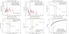 |
Fig. 6. Radial profiles of PLCKG287 obtained from the Chandra spectral analysis. Top panels: temperature (left) and metallicity (middle) from the projected (black) and deprojected (red) spectral analysis; the right panel shows the deprojected density (see Tables B.1 and B.2). Bottom panels: Pressure (left), entropy (middle), and integrated gas mass (right, red points) from the deprojected spectral analysis (see Table B.2). The total mass profile (right, solid black line) was estimated from the circular β-model by assuming an isothermal kT ∼ 12.7 keV. In all panels, the vertical lines show the position of the fronts discussed in Sect. 4 (the dashed blue line and solid red line indicate the cold front and shock, respectively). |
The spectral properties thus derived are the emission-weighted superposition of radiation originating at all points along the line of sight through the cluster atmosphere. In order to account for projection effects, we further performed a deprojection analysis by considering the model projct*tbabs*apec, in which the first component performs a 3D to 2D projection of ellipsoidal shells on to elliptical annuli. The high number of parameters in the projct model requires high photon statistics; therefore, we binned the annuli two by two (but the last one).
We also estimated various quantities derived from the deprojected spectral fits. The electron density ne is obtained from the emission integral EI = ∫nenp dV given by the apec normalization, norm = 10−14EI/(4π[DA(1 + z)]2). We assumed ne ∼ 1.2np in the ionized intra-cluster plasma (e.g., Gitti et al. 2012). By starting from the deprojected density and temperature values, we then calculated the gas pressure as p = nkT, where we assumed n = ne + np, and the gas entropy from the commonly adopted definition  . The results of the deprojection analysis are reported in Table B.2 and the corresponding deprojected temperature, density, pressure and entropy profiles are shown in Fig. 6. We note in particular an entropy and temperature increase in the very center (r ⪅ 160 kpc). This will be discussed in Sect. 5.
We further measured the gas mass profile by integrating in shells the gas density (estimated from the electron density as ρ = 1.92 μ ne mp, where μ ∼ 0.6 is the mean molecular weight and mp is the proton mass), finding Mgas(< R500)∼1.6 × 10¹⁴ M⊙. As a simple estimate, we also derived the analytical profile of the hydrostatic total mass obtained from the best-fit β-model parameters (see e.g., Eq. (20) of Gitti et al. 2012), by assuming an isothermal value of  keV estimated inside R500 (see Sect. 3.2.1). We consider this a robust approximation of the temperature outside of the cluster core (see Fig. 6, top left panel); therefore, we show the profile only for radial distances ≳160 kpc. We estimated Mtot(< R500)≈1.2 × 10¹⁵ M⊙, in agreement with the nominal integrated mass estimated from Planck SZ data (∼1.4 × 10¹⁵ M⊙, Planck Collaboration XXVII 2016). The mass profiles are shown in Fig. 6 (bottom right panel).
3.2.3. 2D spectral maps of ICM thermodynamic properties
To enable high-resolution 2D mapping of the ICM thermodynamic properties, we built maps by using the contour binning technique (CONTBIN, Sanders 2006) and setting8 a minimum signal-to-noise ratio (S/N) of 55. The spectrum extracted from each region was fit with a tbabs * apec model, leaving the temperature, abundance, and normalization free to vary. Consistently with the previous analysis (Sects. 3.2.1 and 3.2.2), the absorbing column density was fixed at the value NH = 6.93 × 1020 cm−2 (HI4PI Collaboration 2016). By combining the temperature and normalization, we further derived maps of pseudo-pressure and pseudo-entropy (in arbitrary units) using the method described in the literature (e.g., Ubertosi et al. 2023).
The resulting maps (Fig. 7) show that the higher abundance gas is preferentially found inside the central ∼300 kpc from the X-ray peak and is bounded by a region of cold gas, which is in turn externally surrounded by a region of hot gas. This hot ICM region is narrower (∼90 kpc) toward the NW direction and corresponds to a region of higher ICM pressure, possibly indicating shock compression. Across the internal cold ICM region the pressure is instead nearly constant, suggesting the presence of a contact discontinuity (cold front). These features will be further investigated in Sect. 4 by means of dedicated morphological and spectral analyses of the radial profiles.
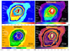 |
Fig. 7. Spectral maps of the ICM thermodynamical properties in PLCKG287 (see Sect. 3.2.3 for details) with overlaid the GMRT radio contours at 330 MHz (same as in Fig. 2). Upper panels: temperature (keV) and pseudo-pressure (arbitrary units) maps. Bottom panels: pseudo-entropy (arbitrary units) and abundance (solar units) maps. The dashed arcs (indicated in different colors in the various panels to enhance visibility depending on the color scale adopted) mark the positions of the surface brightness edges detected in Sect. 4. All maps are centered in the X-ray peak, whereas the cross indicates the location of the main BCG. |
4. Study of the surface brightness discontinuities
We investigated the presence and nature of possible surface brightness discontinuities by performing detailed morphological and spectral analyses of the radial profiles along different sectors. The strategy we adopted was to first estimate the exact position and magnitude of density jumps by studying the surface brightness profile across each edge and then measure the thermodynamic properties (in particular temperature and pressure) inside and outside the front to determine its nature.
In particular, we performed a systematic search for edges in the ICM by extracting surface brightness profiles (centered on the X-ray peak)9 in circular or elliptical sectors of varying opening angles (between 30° and 180°) and different binning (between 1″ and 3″). The resulting profiles were fit in pyproffit with a single power-law model and with a broken power-law model: a surface brightness edge at a distance, RJ, characterized by a density jump, J, was considered a detection if an F-test between the single and the broken power law indicated a significant statistical improvement (more than 99% confidence).
The best-fit results were obtained in sectors in the NW direction (see Fig. 8). We detected an inner edge in a 180°-wide sector (from −57° to +123° from W and increasing counterclockwise) at Rinner = 0.94′±0.02′ = 56.4″ ± 1.2″ ∼ 295 ± 6 kpc from the center, characterized by a density jump Jinner = 1.44 ± 0.08 (χ2/d.o.f. = 53.0/51). We also detected an outer edge in a 80°-wide sector (included in the previous semicircle, from 0° to 80° from W and increasing counterclockwise) at Router = 1.24′±0.02 = 74.4″ ± 1.2″ ∼ 389 ± 6 kpc from the center, characterized by a density jump Jouter = 1.43 ± 0.10 (χ2/d.o.f. = 24.2/24). We verified that slightly varying the radial binning and sector aperture of the profile extraction always provided consistent results.
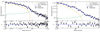 |
Fig. 8. Surface brightness profiles across the NW direction in a semicircle (from −57° to +123° from W and increasing counterclockwise, left panel) and in a narrower 80°-wide sector (from 0° to 80° from W and increasing counterclockwise, right panel). In each panel, the best-fit broken power-law model is overlaid in blue, while the residuals are shown in the lower boxes and the individual components of the SB associated with the broken power law inside (“In”) and outside (“Out”) the front are shown with dashed orange and green lines, respectively. As is discussed in the text, we interpret the inner edge (left panel, Rinner = 0.94′±0.02′∼295 ± 6 kpc) as a cold front and the outer edge (right panel, Router = 1.24′±0.02′∼389 ± 6 kpc) as a shock front. The radial distances are in units of arcmin, where 1 arcmin = 313.8 kpc. |
Given the geometry of the two nested fronts, which are aligned in the same direction, we measured their spectral properties along the common sector having an opening angle of 80° (from 0° to 80° from W and increasing counterclockwise), that is the one in which the outer front is detected. In particular, we extracted the spectra of the ICM inside and outside each discontinuity, with the addition of a central region and an outermost region extending up to R500 to account for deprojection, for a total of 5 spectral wedges. Fitting the 0.5–7.0 keV band spectra with a projct*tbabs*apec model returned the deprojected temperature and electron density, which were combined to derive the pressure jump across each edge. A summary of the deprojected thermodynamic properties along the considered sector is reported in Table 3.
Across the inner edge, located at ∼295 kpc, we measure a temperature jump,  , and a pressure jump,
  . These values are consistent with the interpretation of this edge as a cold front, that is, a contact discontinuity characterized by a continuous pressure and a lower temperature inside the front.
On the other hand, across the outer edge located at ∼389 kpc we measure a temperature jump,  , and pressure jump,
  . These values are consistent with the interpretation of this edge as a shock front that has increased the temperature10 and pressure of the ICM after its passage. By using the Rankine – Hugoniot (R–H) conditions (e.g., Landau & Lifshitz 1960), we estimated the Mach number, ℳ, of the shock front from the best-fit density jump (Jouter = 1.43 ± 0.10) detected in the surface brightness edge as
 (3)
(3)
finding a value of ℳ = 1.29 ± 0.07 (ignoring systematic errors such as projection and sector choice).
Moreover, the Mach number can be used to predict the expected temperature jump across the post- and pre-shock region by again using the R–H conditions:
 (4)
(4)
finding a value of (1.28 ± 0.07), which is consistent with the observed temperature jump ( ).
).
The shock velocity is vshock = ℳ cs, where  is the sound speed in the upstream (pre-shocked) gas. By considering the upstream temperature (kTin = 10.26 keV), we estimated vsh ≈ 2100 km s−1. The properties of the detected shock front are summarized in Tab. 4.
Shock properties.
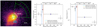 |
Fig. 9. Spectral analysis of the shock and cold fronts in PLCKG287. Left panel: mosaic [0.5–7.0] keV Chandra image of the central region of PLCKG287 smoothed with a kernel of 5 pixels showing the wedges used for the spectral analysis of the surface brightness edges. The white arc and the dashed cyan semicircle indicate the positions of the identified shock and cold front, respectively. Middle and right panels: deprojected temperature (middle) and pressure (right) profiles measured along the wedges shown in the left panel. The vertical lines show the position of the fronts identified in Sect. 4; in particular, the dashed blue line and solid red line indicate the cold front and shock, respectively. |
5. Discussion
The morphological and spectral analyses presented in the previous sections clearly show the presence of a shock front and hot cluster core with high metallicity. A possible interpretation is that some heating event has increased the temperature of the cluster central region, which we argue was previously a cool core.
5.1. The possibility of a former cool core
The interpretation that PLCKG287 hosts a former cool core is mainly supported by the presence of a central peak in the metallicity profile, which is consistent with what is typically observed in samples of relaxed clusters (e.g., De Grandi & Molendi 2001; Lovisari & Reiprich 2019; Ghizzardi et al. 2021). As a comparison, Fig. 10 (right panel) shows the projected metallicity profile of a sample of relaxed clusters observed with BeppoSAX (De Grandi & Molendi 2001), rescaled to the virial radius, Rvir (estimated from Evrard et al. 1996). A strong enhancement in the abundance is found in the central regions. Overlaid is the metallicity profile that we measure for PLCKG287 (red triangles). Despite the large error bars, we note that it is fully consistent with the strong central enhancement in the abundance exhibited by relaxed clusters, supporting the interpretation of PLCKG287 being a former cool core11. In particular, from the spectral fits in the corresponding annular regions we measure Z = 0.57 ± 0.17 Z⊙ inside 0.05 Rvir (r < 30″) compared to Z = 0.27 ± 0.06 Z⊙ in a region with bounding radii of 0.05 Rvir and ∼0.2 Rvir (30″ < r < 120″), where Rvir ∼ 3.1 Mpc for PLCKG287.
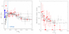 |
Fig. 10. Temperature and metallicity profile of PLCKG287 compared to those of typical relaxed clusters. Left panel: temperature profiles measured for a sample of relaxed clusters presented by Vikhlinin et al. (2005). The temperatures are scaled to the cluster emission-weighted temperature excluding the central 70 kpc regions, ⟨kTX⟩. The profiles for all clusters are projected and scaled in radial units of the virial radius Rvir, as estimated from the relation |


We present below some simple order-of-magnitude energetic estimates to test the scenario in which the inner region of PLCKG287, where we measure a high density and an abundance peak, was the cluster cool core, which has then been heated. In particular, we first estimate the energy required to heat the core (Sect. 5.2) and compare it with that possibly provided by shock heating (Sect. 5.3) and AGN heating (Sect. 5.4), and then discuss the possible origin of the detected shock (Sect. 5.5). We do not attempt to develop or discuss detailed hydrodynamic models, which is beyond the aim of this work; rather, we limit our discussion to energetic considerations only.
5.2. Energy required to heat the core
To obtain a rough estimate of the temperature of the original cool core, which we interpret as the initial temperature before the heating event, we adopted a basic approach based on the comparison with the typical profile of relaxed clusters. In particular, we show in Fig. 10 (left panel) the projected temperature profile of PLCKG287 (red triangles) overlaid to the temperature profiles of a sample of relaxed clusters (Vikhlinin et al. 2005). The radial distances are scaled to the virial radius and the temperatures are scaled to the emission-weighted cluster temperature, excluding the central 70 kpc region usually affected by radiative cooling. To be consistent with the widely adopted scaled profiles presented by Vikhlinin et al. (2005), we thus estimated the emission-weighted temperature used for the scaling of PLCKG287 by excluding the central bin (see Table B.1). We note that the overall temperature profile measured for PLCKG287 is generally consistent within the scatter of the profiles observed in a relaxed cluster for radial distances of r ≳ 0.05 Rvir, corresponding to a physical scale of r ⪆ 160 kpc. On the other hand, in the central region there is a clear departure from the typical profile, with an opposite radial trend12.
In particular, for radial distances of r ⪅ 160 kpc, PLCKG287 shows a negative gradient dT/dr with higher temperatures (scaled kT > 1) with respect to the typical central trend, which instead shows a positive gradient dT/dr and lower temperatures (scaled kT < 1). In our interpretation, the region inside ∼160 kpc thus corresponds to the heated cool core, where we estimated an average core temperature of ∼17 keV (by fitting the combined spectra of the two innermost bins; see Table B.1). On the other hand, by assuming that the original cool core in PLCKG287 featured the typical temperature drop in the central regions observed for relaxed clusters, we estimated that the average pre-heated temperature of PLCKG287 inside ⪅160 kpc was initially below ∼12 keV, reaching local values as low as ≈5 keV in the very center (see Fig. 10, left panel). Therefore, the heating event raised the average ICM temperature in the core by at least 5 keV, from the initial value ≲12 keV to the currently observed value of ∼17 keV.
We verified that the results are not affected by the spherical assumption: we performed a new spectral analysis by considering elliptical annular bins with the same geometry as that of the elliptical β-model (see Table 2). In particular, we extracted spectra in a central ellipse (with major axis ∼160 kpc) and in an adjacent elliptical annulus (with major axis ∼160–300 kpc), finding that the measured temperature and metallicity values are consistent within 1σ to the ones derived in circular bins. We further note that the high temperature values measured by Chandra are consistent with those measured also by XMM-Newton (PLCKG287 is the most massive and hottest cluster in the CHEX-MATE sample: see the red points in Fig. 3, right panel, of Riva et al. 2024)13.
The energy required to increase the ICM temperature by kΔT ≈ 5 keV can be measured as
 (5)
(5)
where Mgas is the gas mass derived by integrating the electron density (see Table B.2) in shells. We obtained a gas mass of Mgas ∼ 1.9 × 10¹² M⊙ inside the central ≈160 kpc (which is the region corresponding to the heated cool core), leading to an estimate of Eheat ≈ 4 × 1061 erg.
5.3. Energy of the shock
In order to verify whether the detected shock can be responsible for heating the cluster core, we need to compare Eheat (just derived in Sect. 5.2) with the energy that has been dumped by the shock. A lower limit for the shock energy, Esh, can be estimated as (e.g., David et al. 2001)
 (6)
(6)
where ppost and ppre are the pressures in the post-shock and pre-shock regions, respectively, and Vsh is the volume of shocked gas. By substituting the expression for the pressure jump expected from the R–H conditions:
 (7)
(7)
we can express the shock energy as a function of the measured post-shock pressure and Mach number as
 (8)
(8)
As the volume of shocked gas, we considered the volume of a sphere of radius Rsh = Router ∼ 389 kpc, reduced by a fiducial factor f that depends on the fraction of the volume occupied by the shocked gas. We therefore estimate a volume of shocked gas of the order of Vsh = 4/3πfRsh3 ∼ 2.5 f × 108 kpc3, where f can range from ∼0.1 to 1 depending on the actual geometry of the shock (f ∼ 0.12 for a shock that propagated through the cluster only along the ∼1.5 steradian solid angle corresponding to the limited projected angle of 80° in which we detected it, and f = 1 for an isotropic shock). Considering the Mach number and post-shock pressure estimated in Sect. 4 (see Table 3), we finally estimated a shock energy Esh ≈ 8 f × 1062 erg, which results of the order of Esh ≈ 1062 erg if f ∼ 0.12. The shock properties are summarized in Tab. 4.
Comparing this with the energy required to heat the core (Eheat ≈ 4 × 1061; see Sect. 5.2), we conclude that even considering the lower limit of the geometrical factor f ∼ 0.12 (that is, considering that the shock propagated through the cluster only in the direction in which we detect it), the amount of energy injected by the shock is a factor ≳ 2 higher than that required to heat the core. In the case of a semispheric or isotropic shock (f = 0.5 or 1), its energy would still be enough to heat the whole region inside the shock radius (Rsh∼ 390 kpc), where we estimated a gas mass of 1.9 × 10¹³ M⊙ and an energy required to heat it of Eheat ≈ 2 × 1062 erg (considering a kΔT ≈ 2 keV estimated from the comparison with the typical temperature profile, Fig. 10). In summary, despite the uncertainties and approximations of our estimates, there are clear indications that the shock injects sufficient energy to overheat the core in PLCKG287.
However, this scenario seems viable only if the shock originated in the cluster center where it was stronger in the past, which could be the case if the central AGN had driven it. On the contrary, it seems implausible that a large-scale merger shock would preferentially heat the former dense cool core. In fact, from Fig. 10 (left panel) we see that ΔT is largest at the center, right where the gas density is the highest. In particular, at r ∼ 0 the observed temperature is a factor of ∼3 higher than that of the typical cool cores. Such a temperature jump would imply a shock with Mach number ℳ ∼ 2, significantly stronger than the shock that is heating gas at larger radii. We investigate the possible origin of the detected shock in Sect. 5.5.
5.4. Energy of AGN feedback
As we discussed in Sect. 5.1, we argue that PLCKG287 is a former cool core. Furthermore, the visual inspection of both the residual and the background-subtracted, exposure-corrected mosaic images revealed the presence of X-ray depressions (see Figs. 5 and A.1). We also note that the locations of the two depressions are opposite with respect to the central radio source associated with the BCG (white contours overlapping the green cross indicating the BCG in Fig. 11). From the GMRT radio data (Bonafede et al. 2014), we estimated that at 610 MHz the BCG has a flux density of ∼2.4 mJy, with a spectral index14α∼ 0.9 calculated between 610 MHz and 323 MHz. This corresponds to a radio power15 of ∼1.2 × 1024 W Hz−1. By extrapolating, assuming a straight spectral index of ∼0.9 up to higher frequencies, we estimated a total flux density of 1.2 mJy at 1.3 GHz, corresponding to a radio power of ∼6 × 10²³ W Hz−1. These results, which are confirmed by new wideband radio observations obtained in L and S bands with MeerKAT in the frequency range ∼1 − 3 GHz (Balboni et al. in prep.; Rajpurohit in prep.), indicate that the BCG hosts a radio AGN, thus corroborating the interpretation of the X-ray depressions as possible cavities. If confirmed, this would be the signature of AGN feedback and thus possibly point to an AGN-driven origin of the heating event.
Assuming that the X-ray depressions are cavities carved by a past AGN outburst, we calculated the cavity properties (summarized in Table 5) and compared them with the energy estimated in Sect. 5.2. In particular, based on the volume V of the cavities estimated from the ellipsoidal shapes indicated in Fig. 5, and on the pressure p of the surrounding hot gas derived from the deprojected spectral analysis (see Table B.2), we estimated that the energy required to inflate them is Ecav ≈ 4 × 1061 erg, where we assumed the typically adopted value of 4pV of energy per cavity (e.g., McNamara & Nulsen 2007). This quantity, which is typically considered a proxy (likely a factor of a few lower) of the total AGN outburst mechanical energy, (e.g., Bîrzan et al. 2004; McNamara & Nulsen 2007; Gitti et al. 2012; Fabian 2012), is comparable to the energy required to heat the former cool core (see Sect. 5.2), thus indicating that AGN feedback may be energetically responsible for overheating the core. This is consistent with simulation results indicating that if a substantial portion of energy from the most energetic AGN outbursts (1061 − 1062 erg, as in PLCK287) is deposited near the centers of cool core clusters, which is a likely scenario given the dense cores, these AGN outbursts can completely remove the cool cores, thereby transforming them into non-cool core clusters (Guo & Mathews 2010).
5.5. Origin of the shock
We discuss below two alternative scenarios for the origin of the detected shock: the origin by merger and the origin by the same AGN outburst that generated the X-ray cavities.
5.5.1. Merger
In the X-ray morphological analysis of the CHEX-MATE sample, PLCKG287 is classified as “mixed” in terms of morphological disturbance (Campitiello et al. 2022). The dynamically active nature of PLCK287 is probed by the presence of two radio relics and a radio halo (Bagchi et al. 2011; Bonafede et al. 2014), but the merger scenario is still not clear (e.g., Golovich et al. 2019). Subaru and HST weak-lensing analysis detected multiple peaks in the mass distribution of PLCKG287, revealing the complexity of this system (Finner et al. 2017). In particular, the HST mass map shows two mass peaks within the central mass clump, with one primary cluster of mass MNWc = 1.59 × 10¹⁵ M⊙ (labeled NWc in Fig. 11) that is likely to be undergoing a merger with one subcluster of mass MSEc = 1.16 × 10¹⁴ M⊙ located at a projected distance d ∼ 320 kpc to the SE (labeled SEc in Fig. 11). The observation of surface brightness discontinuities in the ICM of merging clusters is particular useful to determine whether a significant component of the merger is occurring on the plane of the sky, as edges are easily hindered by projection effects (e.g., Botteon et al. 2018). The detection of a cold front nested within a shock front in PLCKG287 (see Sect. 4 and Fig. 11) may thus suggest the presence of a collision component along the SE-NW axis where the shock is driven by the merger and is located ahead of the infalling subcluster core, in a similar fashion as the Bullet Cluster (e.g., Markevitch et al. 2002; Clowe et al. 2004).
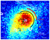 |
Fig. 11. Background-subtracted, exposure corrected mosaic [0.5–7.0] keV Chandra image, smoothed with a kernel of 8 pixels, of the central region of PLCKG287, with superimposed in white the GMRT radio contours at 610 MHz (levels start at ±3σ and increase by a factor of 2, where σ = 0.07 mJy/beam, beam = 6.7″ × 5.3″, Bonafede et al. 2014). The dashed black ellipses show the possible X-ray cavities, whereas the red and black arcs indicates the position of the shock and cold front, respectively. The locations of the X-ray peak and main BCG are indicated by blue and green crosses, respectively, whereas the positions of the dark matter substructures identified by weak lensing analysis are shown by black diamonds and labeled following the same nomenclature as in Finner et al. (2017). |
To investigate the consistency of the merger origin scenario we estimated the energy available during the merger event for heating, that is the energy that can be dissipated in the ICM, and make a comparison with the shock properties. We estimated the merger velocity predicted by free-fall from the turn-around radius of the two subclusters, vmerger, ff, as (e.g., Ricker & Sarazin 2001; Sarazin 2002)
 (9)
(9)
finding an estimate of vmerger ≈ 6800 km/s, which must be considered as an upper limit as d is a projected distance, hence a lower limit to the true separation of the two subclumps. This leads to an estimate of the maximum kinetic energy that can be dissipated in the ICM inside the volume corresponding to the shock distance (∼390 kpc) of
 (10)
(10)
With a gas mass of ∼1.9 × 10¹³ M⊙ inside ∼390 kpc (see Table B.2 and Fig. 6), we thus estimate Ekin, gas ≈ 9 × 1063 erg. This largely exceeds the energy we derived for an isotropic shock (Esh ≈ 8 × 1062 erg; see Table 4), thus the merger scenario is energetically viable. Although these are only order-of-magnitude estimates, based on many assumptions and affected by projection effects, this comparison may further suggest that the shock energy is not fully thermalized, and that some fraction may go into turbulence, magnetic fields, or cosmic rays (e.g., Sarazin 2002), thus powering the diffuse radio sources observed in this cluster (e.g., Bagchi et al. 2011; Bonafede et al. 2014).
On the other hand, the geometry of the shock and cold front system might challenge the merger scenario. The ratio between the stand-off distance Δ = Rsh − Rcf ∼ 94 kpc to the cold front radius Rcf = 295 kpc is ∼0.3, which implies a shock Mach number ℳ ∼ 3, according to the standard theory of shocks generated by a blunt body moving in a uniform medium (e.g., Vikhlinin et al. 2001; Sarazin 2002; Zhang et al. 2019). This finding is at odds with the observed ℳ ∼ 1.3. More recent merging simulations further exacerbate this disagreement, as they show that the ratio Δ/Rcf increases in the post-merger phase reaching typical values Δ/Rcf ∼ 1 − 2 for ℳ ∼ 1.5 − 2 (Zhang et al. 2019). Lower Δ/Rcf values are characteristic only of the pre-merger phase and cannot be applied to PLCKG287 because the observed geometry of the cold front-shock configuration suggests that this is a post-merger system. We therefore investigate the possibility that the shock has a different origin.
5.5.2. AGN outburst
As is discussed in Sect. 5.4, the X-ray depressions can be interpreted as cavities carved by a past AGN outburst and thus possibly point to an AGN-driven origin of the shock, also supported by the fact that the shock is detected in the direction of the cavity pair axis. The AGN outburst origin of the shock would be energetically viable if Ecav is of the same order as Esh or a few times lower, as typically found in systems where both cavity systems and associated shocks were detected (e.g., Randall et al. 2011; Liu et al. 2019; Ubertosi et al. 2023)16. To test the consistency of this scenario, we thus compared the cavity properties with the shock ones. In particular, we note that assuming that the shock propagated only along a limited direction through the cluster (that is the one where we actually detected it, leading to f ∼ 0.12), the energy of the shock (≈1062 erg; see Table 4) would be only a factor of a few higher than that of the cavities (≈4 × 1061 erg; see Table 5). Therefore, the scenario of an AGN origin of the shock is energetically plausible.
We further estimated the cavity age from both the sound crossing time (that is the time necessary to reach the current distance from the center assuming that they are moving at the sound speed) and the expansion time (that is the time necessary to expand to the current size, assuming that they are expanding at the sound speed), resulting in values on the order of 70–80 Myr and ∼40 Myr, respectively. Due to projection effects, these ages must be considered as lower limits. The cavity properties are summarized in Table 5. For comparison, in the scenario of an AGN-driven shock we can estimate an upper limit for its age by considering the time it took to travel from the center to the observed shock radius, Rsh ∼ 390 kpc, at the current shock speed (vsh ≈ 2100 km s−1; see Sect. 4 and Table 4). This results in an estimate of the shock age of tsh = Rsh/vsh≈ 180 Myr, which should be considered as an upper limit because the initial Mach number of the shock was probably higher. Although this upper limit for the shock age might be consistent with the lower limit for the cavity age (⪆40 − 80 Myr), the large difference is a warning against the interpretation of a common origin of both the cavities and shock as due to the central AGN outburst.
We finally note that in general an AGN-driven shock would be able to produce a central temperature peak (e.g., Brighenti & Mathews 2003; Gaspari et al. 2011b,a), as the one observed in PLCKG287, whereas a merger shock would generate a heated region downstream the front where the gas will eventually cool adiabatically as the shock moves in the outskirts (e.g., Heinz et al. 2003; Mathis et al. 2005).
If the AGN heats the gas in the center, it can generate a negative entropy gradient, making the ICM convectively unstable. This is consistent with the entropy profile derived from the deprojected spectral analysis, where we observe an increase of entropy in the central bin. Together with the high density and abundance peak (Fig. 6), this suggests that this structure was the cool core before the heating event (Sect. 5.1). The entropy inversion and pressure drop are indications that the ICM is not relaxed at the center, but it is probably expanding after the AGN heating event. Detailed gas dynamical models would be necessary to validate or disprove this scenario.
6. Summary and conclusions
In this work, we have presented an analysis of new ∼200 ks Chandra observations of the galaxy cluster PLCKG287, which is likely undergoing a merger with a small (∼10% of the mass) subcluster located at a projected distance of ∼320 kpc to the SE (Finner et al. 2017), and which is known to host a giant radio halo and two prominent radio relics in the NW and SE directions at distances of ∼500 kpc and ∼2.8 Mpc from the cluster center (Bonafede et al. 2014). The main results of our detailed morphological and spectral investigations, focused on the region inside R500(∼1.5 Mpc), are summarized below:
-
The cluster shows a comet-like X-ray morphology oriented in the NW-SE direction, with a bright X-ray core region that is co-spatial with the known giant radio halo. The X-ray peak is spatially offset by ∼80 kpc from the main BCG, which is indicative of a disturbed dynamical state. The β-model produces a good fit (Table 2) to the surface brightness profile centered on the X-ray peak, and the residual and unsharp images (Fig. 4) reveal the presence of X-ray depressions to the E and W (Figs. 5 and A.1).
-
From a spectral analysis inside R500, we measure a global temperature of
 keV and abundance of
  Z⊙, with a luminosity of L2 − 10 keV = (1.09 ± 0.01)×1045 erg s−1. The integrated gas mass is Mgas(< R500)∼1.6 × 10¹⁴ M⊙ and the hydrostatic total mass obtained from the best-fit β-model parameters is Mtot(< R500)≈1.2 × 10¹⁵ M⊙.
 -
The radial profile of thermodynamic quantities shows a density, temperature, and abundance peak in the cluster’s center, where the pressure and entropy also undergo a rapid increase (Fig. 6). This is an indication that the ICM is not relaxed at the center, but rather dynamically unstable and probably in expansion. The 2D spectral maps (Fig. 7) further show that the higher abundance gas is preferentially found inside the central ∼300 kpc from the X-ray peak and is bounded by a region of cold gas, which is in turn externally surrounded by a region of hotter gas. This hot ICM region is narrower (∼90 kpc) in the NW direction and corresponds to a region of higher ICM pressure, possibly indicating shock compression. Across the internal cold ICM region the pressure is instead nearly constant, suggesting the presence of a contact discontinuity.
-
By means of accurate morphological and spectral analyses in the regions identified in the residual and spectral maps, we detect a shock front in a 80°-wide sector to the NW at a distance of Rsh = 389 ± 6 kpc from the center, characterized by a density jump of 1.43 ± 0.10, Mach number of ℳ = 1.29 ± 0.07, and shock velocity of vsh ≈ 2100 km s−1. Across the shock, we measure a temperature jump of
 , which is consistent with that expected from the R-H conditions. We estimate a shock energy of Esh ≈ 8 f × 1062 erg, where f is a filling factor indicating the fraction of the volume occupied by the shocked gas (see Table 4 for a summary of the shock properties). We also detect a cold front in a semicircle to the NW at a distance of Rcf = 295 ± 6 kpc from the center, characterized by a density jump of 1.44 ± 0.08 and a temperature jump of
  .
. -
From GMRT radio data, we estimate that the BCG has a 610 MHz radio power of ∼1.2 ×1024 W Hz−1 and a spectral index of α ∼ 0.9, indicating that it hosts a radio AGN. Therefore, the two large depressions detected in the X-ray surface brightness can be most easily explained as the result of an AGN feedback episode. We estimate that the energy associated with the AGN outburst, which occurred ⪆40 Myr ago, is ≳4 × 1061 erg.
-
The observations above point to a scenario in which a heating event has heated a former cool core. The interpretation that PLCKG287 hosted a cool core is mainly supported by the presence of a central peak in the metallicity profile, which is typically observed in samples of cool core clusters (Fig. 10, right panel). By assuming that the original cool core featured the typical temperature drop in the central regions observed for relaxed clusters (Fig. 10, left panel), we estimate that the heating event raised the average ICM temperature in the core (r ⪅ 160 kpc) by approximately 5 keV (see Sect. 5.1), corresponding to an energy of Eheat ≈ 4 × 1061 erg (see Sect. 5.2). Based on simple energetic considerations only, we have explored two scenarios to explain the heated core. In the first case, the detected shock crossed the core region, raising the core temperature by ∼5 keV. Our approximate estimate for the shock energy indicates that this picture is plausible. In the second model, an AGN outburst heats the core from inside out, but no attempt is made to single out the specific heating process (likely still a shock, although not necessarily the one we detect). We estimate that the energy associated with the X-ray cavity formation is again of the same order as the energy required to heat the former cool core. We therefore argue that heating by both the detected shock and by an AGN outburst are energetically viable scenarios (see Table 6 for a summary of the energy estimates). However, we briefly discuss how neither of the scenarios alone seems able to explain all the observed features of the X ray emission in PLCKG287.
-
We discuss the possible origin of the detected shock by investigating the alternative scenarios of (i) merger, which is supported by the observed configuration of a cold front nested inside a shock along the same direction, as is typically expected to be produced during merging processes (Sect. 5.5.1); and (ii) AGN feedback, which is supported by the presence of X-ray cavities in opposite positions with respect to the central radio BCG along the direction of the shock, as is expected if both the cavities and shock are produced by a central AGN outburst (Sect. 5.5.2). We find that both scenarios are energetically viable (see Table 6), although timescale considerations favor a merger origin of the shock.
We finally note that although the merging scenario is more plausible for explaining the origin of the detected shock and particularly the large-scale structure observed in PLCKG287, a merger event is not expected to produce an increase in the central temperature and entropy. This can instead be produced on smaller scales by AGN feedback. Therefore, the observed temperature and entropy peaks that we measure in the core could indicate the concomitant effect of the central AGN, pointing to the combined action of merging and AGN feedback in heating the former cool core of this system. More generally, this indicates that mergers are not solely responsible for disrupting cool cores and that AGN feedback may contribute to shaping the thermodynamical properties of clusters.
Energy estimates presented in this work.
We assumed psfecf = 0.9.
The exposure map was normalized by its value at the aimpoint, resulting in units of seconds as requested by pyproffit.
We show the spectral maps that we consider the best ones after trying different sets of parameters.
We also considered sectors with offset centers in order to better represent the shape of the features visually identified, finding consistent results.
We verified that the temperature jump is detected also in the projected spectral fit:  keV vs.
  keV.
keV.
It is now well established that dynamically disturbed clusters also show an increase in metallicity in the center, although not at the level of the peak in relaxed clusters (see e.g., Leccardi et al. 2010; Lovisari & Reiprich 2019, for a recent measurement on a large sample of objects). However, Rossetti & Molendi (2010) argue that this is due to the presence of cool core remnants, thus still supporting our interpretation.
A similar result comes from the comparison with the temperature profiles derived for the clusters of the CHEX-MATE sample (Rossetti et al. 2024).
Even though cross-calibration differences may exist (as for example the level of 10–15% estimated by Wallbank et al. 2022), the comparison with the temperatures measured in various systems by NuSTAR, with a much broader energy range, confirms the ability of Chandra to measure high temperature values.
We define the spectral index, α, as Sν ∝ ν−α, where Sν is the flux density at the frequency ν.
The monochromatic radio power at the frequency ν is estimated from Pν = 4π DL2 Sν (1 + z)(α − 1) (e.g., Condon & Matthews 2018).
Some exceptions have been observed in which the shock is not the dominant heating source (e.g., Forman et al. 2020).
We verified that the temperature jump is detected also in the projected spectral fit:  keV vs.
  keV.
keV.
Acknowledgments
We thank the anonymous referee for insightful comments and constructive suggestions which stimulated a critical discussion of the results. MG and FU acknowledge support from the research project PRIN 2022 “AGN-sCAN: zooming-in on the AGN-galaxy connection since the cosmic noon”, contract 2022JZJBHM_002 – CUP J53D23001610006. RJvW acknowledges support from the ERC Starting Grant ClusterWeb 804208. MB acknowledges funding by the Deutsche Forschungsgemeinschaft (DFG) under Germany’s Excellence Strategy – EXC 2121 “Quantum Universe” – 390833306 and the DFG Research Group “Relativistic Jets”. WF acknowleges support from the Smithsonian Institution, the Chandra High Resolution Camera Project through NASA contract NAS8-0306, NASA Grant 80NSSC19K0116 and Chandra Grant GO1-22132X. KR acknowledges the Smithsonian Combined Support for Life on a Sustainable Planet, Science, and Research administered by the Office of the Under Secretary for Science and Research. This research has made use of data obtained from the Chandra Data Archive and Chandra Source Catalog and software provided by the Chandra X-ray Center (CXC) in the application packages CIAO. The National Radio Astronomy Observatory is a facility of the National Science Foundation operated under cooperative agreement by Asso-ciated Universities, Inc. Facilities: CXO Software: astropy (Astropy Collaboration 2013, 2018), APLpy (Robitaille & Bressert 2012), Numpy (van der Walt et al. 2011; Harris et al. 2020), CIAO (Fruscione et al. 2006), XSPEC (Arnaud 1996).
References
- Arnaud, K. A. 1996, in Astronomical Data Analysis Software and Systems V, eds. G. H. Jacoby, & J. Barnes, ASP Conf. Ser., 101, 17 [NASA ADS] [Google Scholar]
- Asplund, M., Grevesse, N., Sauval, A. J., & Scott, P. 2009, ARA&A, 47, 481 [NASA ADS] [CrossRef] [Google Scholar]
- Astropy Collaboration (Robitaille, T. P., et al.) 2013, A&A, 558, A33 [NASA ADS] [CrossRef] [EDP Sciences] [Google Scholar]
- Astropy Collaboration (Price-Whelan, A. M., et al.) 2018, AJ, 156, 123 [Google Scholar]
- Bagchi, J., Sirothia, S. K., Werner, N., et al. 2011, ApJ, 736, L8 [NASA ADS] [CrossRef] [Google Scholar]
- Barnes, D. J., Vogelsberger, M., Kannan, R., et al. 2018, MNRAS, 481, 1809 [Google Scholar]
- Bîrzan, L., Rafferty, D. A., McNamara, B. R., Wise, M. W., & Nulsen, P. E. J. 2004, ApJ, 607, 800 [Google Scholar]
- Bonafede, A., Intema, H. T., Brüggen, M., et al. 2014, ApJ, 785, 1 [Google Scholar]
- Botteon, A., Gastaldello, F., & Brunetti, G. 2018, MNRAS, 476, 5591 [Google Scholar]
- Brighenti, F., & Mathews, W. G. 2003, ApJ, 587, 580 [Google Scholar]
- Brunetti, G., & Jones, T. W. 2014, International Journal of Modern Physics D, 23, 30007 [Google Scholar]
- Campitiello, M. G., Ettori, S., Lovisari, L., et al. 2022, A&A, 665, A117 [NASA ADS] [CrossRef] [EDP Sciences] [Google Scholar]
- CHEX-MATE Collaboration (Arnaud, M., et al.) 2021, A&A, 650, A104 [NASA ADS] [CrossRef] [EDP Sciences] [Google Scholar]
- Clowe, D., Gonzalez, A., & Markevitch, M. 2004, ApJ, 604, 596 [NASA ADS] [CrossRef] [Google Scholar]
- Condon, J. J., & Matthews, A. M. 2018, PASP, 130 [Google Scholar]
- D’Addona, M., Mercurio, A., Rosati, P., et al. 2024, A&A, 686, A4 [NASA ADS] [CrossRef] [EDP Sciences] [Google Scholar]
- David, L. P., Nulsen, P. E. J., McNamara, B. R., et al. 2001, ApJ, 557, 546 [CrossRef] [Google Scholar]
- De Grandi, S., & Molendi, S. 2001, ApJ, 551, 153 [NASA ADS] [CrossRef] [Google Scholar]
- Dolag, K., Bykov, A. M., & Diaferio, A. 2008, Space Sci. Rev., 134, 311 [NASA ADS] [CrossRef] [Google Scholar]
- Douglass, E. M., Blanton, E. L., Randall, S. W., et al. 2018, ApJ, 868, 121 [Google Scholar]
- Eckert, D., Molendi, S., & Paltani, S. 2011, A&A, 526, A79 [NASA ADS] [CrossRef] [EDP Sciences] [Google Scholar]
- Eckert, D., Finoguenov, A., Ghirardini, V., et al. 2020, The Open Journal of Astrophysics, 3, 12 [CrossRef] [Google Scholar]
- Evrard, A. E., Metzler, C. A., & Navarro, J. F. 1996, ApJ, 469, 494 [Google Scholar]
- Fabian, A. C. 2012, ARA&A, 50, 455 [Google Scholar]
- Finner, K., Jee, M. J., Golovich, N., et al. 2017, ApJ, 851, 46 [NASA ADS] [CrossRef] [Google Scholar]
- Finner, K., Jee, M. J., Cho, H., et al. 2024, ApJ, submitted [arXiv:2407.02557] [Google Scholar]
- Forman, W., Churazov, E., Heinz, S., et al. 2020, in Perseus in Sicily: From Black Hole to Cluster Outskirts, eds. K. Asada, E. de Gouveia Dal Pino, M. Giroletti, H. Nagai, & R. Nemmen, IAU Symposium, 342, 112 [Google Scholar]
- Fruscione, A., McDowell, J. C., Allen, G. E., et al. 2006, in Observatory Operations: Strategies, Processes, and Systems, eds. D. R. Silva, & R. E. Doxsey, SPIE Conf. Ser., 6270, 62701V [NASA ADS] [CrossRef] [Google Scholar]
- Gaspari, M., Brighenti, F., D’Ercole, A., & Melioli, C. 2011a, MNRAS, 415, 1549 [NASA ADS] [CrossRef] [Google Scholar]
- Gaspari, M., Melioli, C., Brighenti, F., & D’Ercole, A. 2011b, MNRAS, 411, 349 [Google Scholar]
- Ghizzardi, S., Molendi, S., van der Burg, R., et al. 2021, A&A, 646, A92 [NASA ADS] [CrossRef] [EDP Sciences] [Google Scholar]
- Gitti, M., Brighenti, F., & McNamara, B. R. 2012, Advances in Astronomy, 2012 [Google Scholar]
- Golovich, N., Dawson, W. A., Wittman, D. M., et al. 2019, ApJ, 882, 69 [NASA ADS] [CrossRef] [Google Scholar]
- Guo, F., & Mathews, W. G. 2010, ApJ, 717, 937 [Google Scholar]
- Harris, C. R., Millman, K. J., van der Walt, S. J., et al. 2020, Nature, 585, 357 [NASA ADS] [CrossRef] [Google Scholar]
- Heinz, S., Churazov, E., Forman, W., Jones, C., & Briel, U. G. 2003, MNRAS, 346, 13 [NASA ADS] [CrossRef] [Google Scholar]
- HI4PI Collaboration (Ben Bekhti, N., et al.) 2016, A&A, 594, A116 [NASA ADS] [CrossRef] [EDP Sciences] [Google Scholar]
- Kravtsov, A. V., & Borgani, S. 2012, ARA&A, 50, 353 [Google Scholar]
- Landau, L. D., & Lifshitz, E. M. 1960, Electrodynamics of Continuous Media (Pergamon Press) [Google Scholar]
- Leccardi, A., Rossetti, M., & Molendi, S. 2010, A&A, 510, A82 [NASA ADS] [CrossRef] [EDP Sciences] [Google Scholar]
- Liu, W., Sun, M., Nulsen, P., et al. 2019, MNRAS, 484, 3376 [NASA ADS] [CrossRef] [Google Scholar]
- Lovisari, L., & Reiprich, T. H. 2019, MNRAS, 483, 540 [Google Scholar]
- Markevitch, M., Gonzalez, A. H., David, L., et al. 2002, ApJ, 567, L27 [Google Scholar]
- Mathis, H., Lavaux, G., Diego, J. M., & Silk, J. 2005, MNRAS, 357, 801 [Google Scholar]
- McCarthy, I. G., Babul, A., Bower, R. G., & Balogh, M. L. 2008, MNRAS, 386, 1309 [NASA ADS] [CrossRef] [Google Scholar]
- McNamara, B. R., & Nulsen, P. E. J. 2007, ARA&A, 45, 117 [NASA ADS] [CrossRef] [Google Scholar]
- Molendi, S., De Grandi, S., Rossetti, M., et al. 2023, A&A, 670, A104 [NASA ADS] [CrossRef] [EDP Sciences] [Google Scholar]
- Petrosian, V., & Bykov, A. M. 2008, Space Sci. Rev., 134, 207 [NASA ADS] [CrossRef] [Google Scholar]
- Planck Collaboration XXVII. 2016, A&A, 594, A27 [NASA ADS] [CrossRef] [EDP Sciences] [Google Scholar]
- Randall, S. W., Forman, W. R., Giacintucci, S., et al. 2011, ApJ, 726, 86 [NASA ADS] [CrossRef] [Google Scholar]
- Rasia, E., Borgani, S., Murante, G., et al. 2015, ApJ, 813, L17 [Google Scholar]
- Ricker, P. M., & Sarazin, C. L. 2001, ApJ, 561, 621 [NASA ADS] [CrossRef] [Google Scholar]
- Riva, G., Pratt, G. W., Rossetti, M., et al. 2024, A&A, 691, A340 [NASA ADS] [CrossRef] [EDP Sciences] [Google Scholar]
- Robitaille, T., & Bressert, E. 2012, Astrophysics Source Code Library [record ascl:1208.017] [Google Scholar]
- Rossetti, M., & Molendi, S. 2010, A&A, 510, A83 [NASA ADS] [CrossRef] [EDP Sciences] [Google Scholar]
- Rossetti, M., Gastaldello, F., Ferioli, G., et al. 2016, MNRAS, 457, 4515 [Google Scholar]
- Rossetti, M., Eckert, D., Gastaldello, F., et al. 2024, A&A, 686, A68 [NASA ADS] [CrossRef] [EDP Sciences] [Google Scholar]
- Sanders, J. S. 2006, MNRAS, 371, 829 [Google Scholar]
- Sarazin, C. L. 2002, in Merging Processes in Galaxy Clusters, eds. L. Feretti, I. M. Gioia, & G. Giovannini, Astrophysics and Space Science Library, 272, 1 [NASA ADS] [Google Scholar]
- Schellenberger, G., O’Sullivan, E., Giacintucci, S., et al. 2023, ApJ, 948, 101 [CrossRef] [Google Scholar]
- Stuardi, C., Bonafede, A., Rajpurohit, K., et al. 2022, A&A, 666, A8 [Google Scholar]
- Ubertosi, F., Gitti, M., & Brighenti, F. 2023, A&A, 670, A23 [NASA ADS] [CrossRef] [EDP Sciences] [Google Scholar]
- van der Walt, S., Colbert, S. C., & Varoquaux, G. 2011, Computing in Science and Engineering, 13, 22 [Google Scholar]
- van Weeren, R. J., de Gasperin, F., Akamatsu, H., et al. 2019, Space Sci. Rev., 215, 16 [Google Scholar]
- Vikhlinin, A., Markevitch, M., & Murray, S. S. 2001, ApJ, 551, 160 [CrossRef] [Google Scholar]
- Vikhlinin, A., Markevitch, M., Murray, S. S., et al. 2005, ApJ, 628, 655 [Google Scholar]
- Vikhlinin, A. A., Kravtsov, A. V., Markevich, M. L., Sunyaev, R. A., & Churazov, E. M. 2014, Physics Uspekhi, 57, 317 [Google Scholar]
- Wallbank, A. N., Maughan, B. J., Gastaldello, F., Potter, C., & Wik, D. R. 2022, MNRAS, 517, 5594 [NASA ADS] [CrossRef] [Google Scholar]
- Zhang, C., Churazov, E., Forman, W. R., & Jones, C. 2019, MNRAS, 482, 20 [NASA ADS] [CrossRef] [Google Scholar]
Appendix A: Analysis of X-ray depressions
We show in Fig. A.1 the sectors used to investigate the significance of the X-ray depressions discussed in Sect. 3.1.
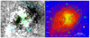 |
Fig. A.1. Surface brightness regions used for the analysis of the depressions in the ICM of PLCKG287. Left panel: Residual Chandra image of the central cluster region obtained by subtracting the best-fit β-model (same as in Fig. 4, left panel) with superimposed the GMRT radio contours at 610 MHz (same as in Fig. 11). The elliptical wedges used to evaluate the azimuthal SB profile around the center were chosen so as to mostly encompass the region of each depression (elliptical annulus between 10″ and 45″ along the major axis, divided in 12 sectors of 30° each) and are shown in green panda regions. The magenta cross indicates the location of the main BCG. Right panel: Background-subtracted, exposure-corrected mosaic [0.5-7.0] keV Chandra image, smoothed with a kernel of 8 pixels, of the same central region of PLCKG287 as in the left panel. The elliptical wedges used to extract the radial SB profile in 5″-wide annular bin along four azimuthal sectors (N: 8° - 108°, E: 108° - 200°, S: 200° - 308°, W: 308° - 368°) are shown in green panda regions (to improve clarity, the annular bins shown in Fig. are 10″-wide instead of 5″-wide). The geometry is the same as that of the elliptical β-model (see Table 2). In both panels, the dashed ellipses show the possible X-ray cavities identified in Sect. 3.1 and discussed in Sect. 5.5.2. |
Appendix B: Spectral analysis with NH fixed to the galactic value
Results of the spectral fit to an absorbed apec model (tbabs*apec) performed in the [0.5-7.0] keV energy band in concentric annular regions extracted up to R500.
Results of the deprojected spectral fit to an absorbed apec model (projct*tbabs*apec) performed in the [0.5-7.0] keV energy band in concentric annular regions extracted up to R500.
Appendix C: Spectral analysis with NH free
We present below the spectral analysis performed with the column density left as a free parameter.
C.1. Global properties inside R500
We first measured the global properties inside R500 by considering a circular region of radius = 294.7″ (= 1541 kpc; see the green circle in Fig. 2). We found that a free value of the galactic hydrogen column parameter, NH, was preferred by the fit (F-stat = 68.85, F-prob = 4.52 × 10⁻¹⁴) over the parameter fixed to the tabulated value of NH = 6.93 × 1020 cm−2 (HI4PI Collaboration 2016). The best-fit parameters are: NH = 1.47 ± 0.10 × 1021 cm−2, temperature  keV and abundance
  Z⊙. With the model tbabs*clumin*apec we estimated the unabsorbed luminosity in the soft, hard and bolometric bands to be L0.3 − 2.4 keV = (6.23 ± 0.03)×1044 erg s−1, L2 − 10 keV = (1.11 ± 0.01)×1045 erg s−1 and Lbol = (2.36 ± 0.01)×1045 erg s−1, respectively. We also verified that the addition of a power-law component (model tbabs*(apec+po)), to account for the presence of unresolved X-ray binaries, is not statistically significant (F-stat = 2.24, F-prob = 0.107). The spectral fitting results are reported in Table C.1.
Results of the spectral fits inside R500.
C.2. 1D radial profiles of ICM thermodynamic properties
In order to derive the azimuthally averaged radial properties of the ICM, we produced projected temperature and abundance profiles by extracting spectra in circular annuli centered on the peak of the X-ray emission. The annular regions were chosen in order to collect at least 3,000-3,500 net counts (see Table C.2). We verified that freeing the column density parameter, linked among the different annuli, provides a better fit (χ2/dof= 2302/2325 = 0.99) than that obtained by fixing it at the tabulated value (χ2/dof= 2390/2326 = 1.03; F-stat= 89.2, F-prob = 9.8 × 10⁻²¹). We found a best-fit value of NH = 1.60 ± 0.10 × 1021 cm−2. The best-fit parameter obtained from the fits to the annular spectra are summarized in Table C.2.
Results of the spectral fit to an absorbed apec model (tbabs*apec) performed in the [0.5-7.0] keV energy band in concentric annular regions extracted up to R500.
C.3. Study of the surface brightness discontinuities
Given the geometry of the two nested fronts, which are aligned along the same direction, we measured their spectral properties along a common sector having an opening angle of 120° (from 0° to 120° from W and increasing counterclockwise). In particular, we extracted the spectra of the ICM inside and outside each discontinuity, with the addition of a central region and an outermost region extending to R500 to account for deprojection, for a total of 5 spectral wedges. Fitting the 0.5-7.0 keV band spectra with a projct*tbabs*apec model (by keeping NH as a free parameter, linked among the different sectors) returned the deprojected temperature and electron density, which were combined to derive the pressure jump across each edge. A summary of the deprojected thermodynamic properties along the considered sector is reported in Table C.3.
Across the inner edge, located at ∼295 kpc, we measure a temperature jump  and a pressure jump
  . These are consistent with the interpretation of this edge as a cold front. On the other hand, across the outer edge located at ∼389 kpc we measure a temperature jump
  and a pressure jump
  . These are consistent with the interpretation of this edge as a shock front17.
Results of the deprojected spectral fit along a 120°-wide sector enclosing the two fronts identified in Sect. 4.
All Tables
Summary of the Chandra ACIS-I observations analyzed in this work (PI: A. Bonafede).
Results of the spectral fit to an absorbed apec model (tbabs*apec) performed in the [0.5-7.0] keV energy band in concentric annular regions extracted up to R500.
Results of the deprojected spectral fit to an absorbed apec model (projct*tbabs*apec) performed in the [0.5-7.0] keV energy band in concentric annular regions extracted up to R500.
Results of the spectral fit to an absorbed apec model (tbabs*apec) performed in the [0.5-7.0] keV energy band in concentric annular regions extracted up to R500.
Results of the deprojected spectral fit along a 120°-wide sector enclosing the two fronts identified in Sect. 4.
All Figures
|
Fig. 1. Field of view of the Chandra observations of PLCKG287 (z = 0.383). Left panel: footprint of the five Chandra ObsIDs. Right panel: background-subtracted, exposure-corrected mosaic in the [0.5–7.0] keV band. The detected point sources that were removed from the analysis are shown with green ellipses. In both panels, the white circle indicates R500 = 1541 kpc, which is the region on which we focus our analysis. |
| In the text | |
|
Fig. 2. Background-subtracted, exposure-corrected Chandra mosaic of PLCKG287 in the [0.5–7.0] keV band smoothed with a kernel of 4 pixels (1 ACIS pixel = 0.492″). The detected point sources (shown with green ellipses in the right panel of Fig. 1) have been subtracted. The green circle indicates R500 = 1541 kpc. Overlaid in white are the GMRT radio contours at 330 MHz (levels start at ±3σ and increase by a factor of 2, where σ = 0.1 mJy/beam, beam = 12.9″ × 7.9″). The radio data shows two prominent radio relics to the NW and SE at distances of ∼500 kpc and ∼2.8 Mpc kpc from the cluster center. The bright X-ray core region is coincident with a giant radio halo. See Bonafede et al. (2014) for more details on the radio features. |
| In the text | |
|
Fig. 3. Background-subtracted, azimuthally averaged radial surface brightness profile in the [0.5–7.0] keV energy band extracted in circular (left panel) and elliptical (right panel) annuli. The best-fit to a single β-model is shown with a blue line in both panels. The best-fit parameters are reported in Table 2. The radial distances are in units of arcmin, where 1 arcmin = 313.8 kpc. |
| In the text | |
|
Fig. 4. Morphological substructures in PLCKG287 from filtered Chandra images. Left panel: residual Chandra image of the central cluster region obtained by subtracting the best-fit elliptical β-model (see Table 2). As is indicated by the color bar, the positive and negative residuals are shown in red and blue, respectively. Right panel: unsharp masked image obtained by subtracting a 40″-smoothed image from a 5″-smoothed one. The dashed green ellipses show the possible X-ray depressions discussed in Sect. 5.4, whereas the red arc indicates the position of the identified shock front (see Sect. 4). Overlaid are the GMRT radio contours at 330 MHz (same as in Fig. 2). In both panels, the black and magenta crosses indicate the location of the X-ray peak (RA 11:50:49.4, Dec −28:04:44.3) and main BCG (RA 11:50:50.2, Dec −28:04:55.7), respectively. |
| In the text | |
|
Fig. 5. Detection of E-W depressions in PLCKG287. Left panel: azimuthal SB profile around the cluster center extracted along the wedges shown in the middle panel. The largest deficit is in the direction of the E depression seen in the residual and unsharp images (see Fig. 4). A second dip is visible in the azimuthal profile in the direction of the W depression. Angles are measured counterclockwise, with 0° to the West direction, and are shown starting from −90° to improve the visibility of the West deficit in the plot. Middle panel: background-subtracted, exposure-corrected mosaic [0.5–7.0] keV Chandra image, smoothed with a kernel of 8 pixels, of the central region of PLCKG287. The elliptical wedges used to evaluate the azimuthal SB profile around the center were chosen so as to mostly encompass the region of each depression (elliptical annulus between 10″ and 45″ along the major axis, divided in 12 sectors of 30° each) and are shown in green panda regions. The dashed black ellipses show the identified X-ray depressions (see also Fig. A.1). Right panel: SB profiles extracted in 5″-wide annular bins (with the same geometry as that used for the elliptical β-model; see Fig. A.1) in four sectors to the N (blue), E (yellow), S (green) and W (red) directions. With respect to the SB profiles in orthogonal directions, a clear depression is visible in the E profile in the radial range ≈0.25′–0.75′, and a smaller deficit is noticeable in the W profile in the radial range ≈0.4′–0.6′. The radial distances are indicated along the major axis, in units of arcmin (1 arcmin = 313.8 kpc). |
| In the text | |
|
Fig. 6. Radial profiles of PLCKG287 obtained from the Chandra spectral analysis. Top panels: temperature (left) and metallicity (middle) from the projected (black) and deprojected (red) spectral analysis; the right panel shows the deprojected density (see Tables B.1 and B.2). Bottom panels: Pressure (left), entropy (middle), and integrated gas mass (right, red points) from the deprojected spectral analysis (see Table B.2). The total mass profile (right, solid black line) was estimated from the circular β-model by assuming an isothermal kT ∼ 12.7 keV. In all panels, the vertical lines show the position of the fronts discussed in Sect. 4 (the dashed blue line and solid red line indicate the cold front and shock, respectively). |
| In the text | |
|
Fig. 7. Spectral maps of the ICM thermodynamical properties in PLCKG287 (see Sect. 3.2.3 for details) with overlaid the GMRT radio contours at 330 MHz (same as in Fig. 2). Upper panels: temperature (keV) and pseudo-pressure (arbitrary units) maps. Bottom panels: pseudo-entropy (arbitrary units) and abundance (solar units) maps. The dashed arcs (indicated in different colors in the various panels to enhance visibility depending on the color scale adopted) mark the positions of the surface brightness edges detected in Sect. 4. All maps are centered in the X-ray peak, whereas the cross indicates the location of the main BCG. |
| In the text | |
|
Fig. 8. Surface brightness profiles across the NW direction in a semicircle (from −57° to +123° from W and increasing counterclockwise, left panel) and in a narrower 80°-wide sector (from 0° to 80° from W and increasing counterclockwise, right panel). In each panel, the best-fit broken power-law model is overlaid in blue, while the residuals are shown in the lower boxes and the individual components of the SB associated with the broken power law inside (“In”) and outside (“Out”) the front are shown with dashed orange and green lines, respectively. As is discussed in the text, we interpret the inner edge (left panel, Rinner = 0.94′±0.02′∼295 ± 6 kpc) as a cold front and the outer edge (right panel, Router = 1.24′±0.02′∼389 ± 6 kpc) as a shock front. The radial distances are in units of arcmin, where 1 arcmin = 313.8 kpc. |
| In the text | |
|
Fig. 9. Spectral analysis of the shock and cold fronts in PLCKG287. Left panel: mosaic [0.5–7.0] keV Chandra image of the central region of PLCKG287 smoothed with a kernel of 5 pixels showing the wedges used for the spectral analysis of the surface brightness edges. The white arc and the dashed cyan semicircle indicate the positions of the identified shock and cold front, respectively. Middle and right panels: deprojected temperature (middle) and pressure (right) profiles measured along the wedges shown in the left panel. The vertical lines show the position of the fronts identified in Sect. 4; in particular, the dashed blue line and solid red line indicate the cold front and shock, respectively. |
| In the text | |
|
Fig. 10. Temperature and metallicity profile of PLCKG287 compared to those of typical relaxed clusters. Left panel: temperature profiles measured for a sample of relaxed clusters presented by Vikhlinin et al. (2005). The temperatures are scaled to the cluster emission-weighted temperature excluding the central 70 kpc regions, ⟨kTX⟩. The profiles for all clusters are projected and scaled in radial units of the virial radius Rvir, as estimated from the relation |
| In the text | |
|
Fig. 11. Background-subtracted, exposure corrected mosaic [0.5–7.0] keV Chandra image, smoothed with a kernel of 8 pixels, of the central region of PLCKG287, with superimposed in white the GMRT radio contours at 610 MHz (levels start at ±3σ and increase by a factor of 2, where σ = 0.07 mJy/beam, beam = 6.7″ × 5.3″, Bonafede et al. 2014). The dashed black ellipses show the possible X-ray cavities, whereas the red and black arcs indicates the position of the shock and cold front, respectively. The locations of the X-ray peak and main BCG are indicated by blue and green crosses, respectively, whereas the positions of the dark matter substructures identified by weak lensing analysis are shown by black diamonds and labeled following the same nomenclature as in Finner et al. (2017). |
| In the text | |
|
Fig. A.1. Surface brightness regions used for the analysis of the depressions in the ICM of PLCKG287. Left panel: Residual Chandra image of the central cluster region obtained by subtracting the best-fit β-model (same as in Fig. 4, left panel) with superimposed the GMRT radio contours at 610 MHz (same as in Fig. 11). The elliptical wedges used to evaluate the azimuthal SB profile around the center were chosen so as to mostly encompass the region of each depression (elliptical annulus between 10″ and 45″ along the major axis, divided in 12 sectors of 30° each) and are shown in green panda regions. The magenta cross indicates the location of the main BCG. Right panel: Background-subtracted, exposure-corrected mosaic [0.5-7.0] keV Chandra image, smoothed with a kernel of 8 pixels, of the same central region of PLCKG287 as in the left panel. The elliptical wedges used to extract the radial SB profile in 5″-wide annular bin along four azimuthal sectors (N: 8° - 108°, E: 108° - 200°, S: 200° - 308°, W: 308° - 368°) are shown in green panda regions (to improve clarity, the annular bins shown in Fig. are 10″-wide instead of 5″-wide). The geometry is the same as that of the elliptical β-model (see Table 2). In both panels, the dashed ellipses show the possible X-ray cavities identified in Sect. 3.1 and discussed in Sect. 5.5.2. |
| In the text | |
Current usage metrics show cumulative count of Article Views (full-text article views including HTML views, PDF and ePub downloads, according to the available data) and Abstracts Views on Vision4Press platform.
Data correspond to usage on the plateform after 2015. The current usage metrics is available 48-96 hours after online publication and is updated daily on week days.
Initial download of the metrics may take a while.