| Issue |
A&A
Volume 693, January 2025
|
|
|---|---|---|
| Article Number | A55 | |
| Number of page(s) | 13 | |
| Section | Cosmology (including clusters of galaxies) | |
| DOI | https://doi.org/10.1051/0004-6361/202452212 | |
| Published online | 03 January 2025 | |
The massive galaxy cluster CL0238.3+2005 (the Peanut cluster) at z = 0.42: A merger just after pericenter passage?
1
Max Planck Institute for Astrophysics, Karl-Schwarzschild-Str. 1, D-85741 Garching, Germany
2
Space Research Institute (IKI), Profsoyuznaya 84/32, Moscow 117997, Russia
3
Universitäts-Sternwarte, Fakultät für Physik, Ludwig-Maximilians-Universität München, Scheinerstr.1, 81679 München, Germany
4
Center for Astrophysics, Harvard & Smithsonian, 60 Garden St, Cambridge, MA 02138, USA
5
Kazan Federal University, Kremlevskaya Str. 18, 420008 Kazan, Russia
6
Tatarstan Academy of Sciences, Bauman Str. 20, 420111 Kazan, Russia
⋆ Corresponding author; This email address is being protected from spambots. You need JavaScript enabled to view it.
Received:
11
September
2024
Accepted:
7
November
2024
Abstract
Massive clusters of galaxies are very rare in the observable Universe. Mergers of such clusters observed close to pericenter passage are even rarer. Here, we report on one such case: The massive (∼1015 M⊙) and hot (kT ∼ 10 keV) cluster CL0238.3+2005 at z = 0.42. For this cluster, we combined X-ray data from SRG/eROSITA and Chandra, optical images from DESI, and spectroscopy from the BTA and RTT-150 telescopes. The X-ray and optical morphologies suggest an ongoing merger with a projected separation of the subhalos of ∼200 kpc. The line-of-sight velocity of galaxies that are tentatively associated with the two merging halos differs by 2000–3000 km s−1. We conclude that the merger axis is most likely neither close to the line of sight nor to the sky plane. We compare CL0238 with the two well-known clusters MACS0416 and the Bullet and conclude that CL0238 corresponds to an intermediate phase between the pre-merging MACS0416 cluster and the post-merger Bullet cluster. Namely, this cluster recently (only ≲0.1 Gyr ago) experienced an almost head-on merger. We argue that this “just after” system is a very rare case and an excellent target for lensing, the Sunyaev-Zeldovich effect, and X-ray studies that can constrain properties ranging from dynamics of mergers to self-interacting dark matter, and plasma effects in the intracluster medium that are associated with shock waves, for instance, electron-ion equilibration efficiency and relativistic particle acceleration.
Key words: galaxies: clusters: intracluster medium / galaxies: distances and redshifts / galaxies: clusters: individual: CL0238.3+2005
© The Authors 2024
 Open Access article, published by EDP Sciences, under the terms of the Creative Commons Attribution License (https://creativecommons.org/licenses/by/4.0), which permits unrestricted use, distribution, and reproduction in any medium, provided the original work is properly cited.
This article is published in open access under the Subscribe to Open model.
Open access funding provided by Max Planck Society.
1. Introduction
The merging of galaxy clusters is a fundamental process in the hierarchical formation of the cosmic web. Galaxy cluster mergers have several distinct phases, from the initial approach and core passage to the post-merger phase and eventual relaxation. Each phase is associated with distinct observational signatures, providing valuable insights into the dynamics of galaxy clusters, dark matter properties (e.g., Markevitch et al. 2004), and microphysics of the plasma, which constitutes the X-ray emitting intracluster medium (see, e.g., Markevitch & Vikhlinin 2007; Zuhone & Roediger 2016), for reviews). On the other hand, perturbations induced by mergers can complicate the use of galaxy cluster samples as cosmological probes. In particular, the cluster number density as a function of their mass and redshift sensitively depends on cosmological parameters (e.g., Kravtsov & Borgani 2012, for a review). However, during mergers, clusters are far from equilibrium, and most approaches for mass estimation give biased results, which in turn bias the resulting cosmological parameters (for instance, Wik et al. 2008; Angrick & Bartelmann 2012).
In this work, we study properties of the massive (∼1015 M⊙) cluster SRGe CL0238.3+2005 (hereafter, we use CL0238 as an acronym for this object) at z ≈ 0.4 using X-ray and optical observations. At first glance, due to its high mass and high luminosity in X-rays (Lx = 6.6 × 1044 erg s−1 in the 0.5–2.0 keV band, as estimated in Burenin et al. 2022), and because of its relatively regular morphology in the low angular resolution ROSAT (e.g., Voges et al. 1999) and Planck (Planck Collaboration XXII 2016) data, CL0238 might appear as a relaxed cluster that is perfectly suited for cosmological studies. However, optical images show a very elongated chain of galaxies. As we show below, new Chandra X-ray observations with a high angular resolution clearly reveal the perturbed state of the cluster. Moreover, CL0238 appears to be in a relatively short-lived merger phase, just after pericenter passage. In combination with its high mass and an intermediate redshift, this makes CL0238 an interesting target for gravitational-lensing studies on par with clusters from the HST Frontier Fields sample (Lotz et al. 2017) and for testing self-interacting dark matter models (e.g. Adhikari et al. 2022, for a recent review), as discussed for the Bullet cluster in Markevitch et al. (2004), Randall et al. (2008) and more recently in a generic context including baryonic effects in Fischer et al. (2023), Sirks et al. (2024).
Burenin et al. (2022) identified the cluster CL0238 in the all-sky survey that was conducted with the eROSITA telescope on board the Spectrum–Roentgen–Gamma (SRG) observatory (Sunyaev et al. 2021; Predehl et al. 2021) and conducted the first spectroscopic observations of the cluster at the 6 m Big Telescope Azimuthal (BTA) telescope in the mode of long-slit spectroscopy. Burenin et al. (2022) measured a cluster redshift z = 0.4205 and estimated its mass as M500 ≈ 9 × 10¹⁴ M⊙ from the X-ray luminosity. Historically, the cluster CL0238 was first detected as an extended X-ray source in the ROSAT All-Sky Survey Faint Source Catalogue (Voges et al. 2000) in the 0.1–2.4 keV energy band. Later, Wen et al. (2012) found a prominent concentration of galaxies in the same area in the Sloan Digital Sky Survey III and assigned it to a cluster with a photometric redshift zphot = 0.4266, and a mass1M500 ∼ 4 × 10¹⁴ M⊙ from the total luminosity of cluster member candidates within the radius of 1 Mpc2. The cluster was also listed in the CompRASS catalog (Tarrio et al. 2019), which is an all-sky catalog of galaxy clusters obtained from the joint analysis of the Planck satellite data and the ROSAT all-sky survey. According to Tarrio et al. (2019), the CL0238 mass is estimated to be  .
.
Here, we analyze SRG/eROSITA, Chandra, and optical observations to shed light on the properties of CL0238. We adopt a Λ cold dark matter cosmology with ΩM = 0.3, ΩΛ = 0.7, and H0 = 70 km s−1 Mpc−1. At the cluster redshift z = 0.4205, 1 arcmin corresponds to 332.2 kpc.
2. Optical observations
Spectroscopic observations of the brightest red-sequence galaxies of the SRGe CL0238.3+2005 cluster were carried out with (1) the 6 m BTA telescope (see Burenin et al. 2022; Zaznobin et al. 2023) and (2) the Russian-Turkish 1.5 m telescope (RTT-150) at the Turkish National Observatories, the Observatory in Antalya, Turkey. Using the multimode SCORPIO and SCORPIO-2 spectrographs (Afanasiev & Moiseev 2005, 2011), Burenin et al. (2022) obtained spectra for two bright galaxies in SRGe CL0238.3+2005 (marked with squares in Fig. 1) and measured their spectroscopic redshifts (see Table 1).
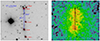 |
Fig. 1. Spectroscopic redshifts of individual galaxies in SRGe CL0238.3+2005. Galaxies observed with the 6 m BTA telescope are marked as squares, and those observed with the 1.5 Russian-Turkish telescope are marked with circles. Measured redshifts (see Table 1) are presented next to symbols (a square or a circle). The left panel shows the RTT-150 composite rizw image (see Sect. 2), and the right panel shows the Chandra image. One subhalo might be associated with four visually clustered galaxies to the north. For the second subhalo, we considered two options: A galaxy with z = 0.4158 that lies within the southern bright X-ray region (see the right panel), and a galaxy with z = 0.4104 that lies between bright X-ray peaks. |
Spectroscopic redshifts of individual galaxies in CL0238.
The RTT-150 observations were carried out in March 7-11, 2024, with the TFOSC instrument and the Andor iKon-L 936 BEX2-DD-9ZQ CCD with a size of 2048 × 2048 pixels, thermoelectrically cooled to – 80°C. The field of view in direct-image mode is 11 × 11 arcmin2 with a scale of 0.33 arcsec/pixel at a binning of 1 × 1. For each observed galaxy, one spectrum with an exposure time of 3600 s was obtained by using grizm 15 and th 134 μ entrance slit (corresponding to 2.4 arcsec on the sky). The wavelength range was 3900–8900 Å, and the spectral resolution was 15 Å (a 2 × 2 binning was used for the spectral observations).
The redshifts of the observed galaxies were determined by cross-correlation with an elliptical galaxy template spectrum3. A detailed description can be found in Khamitov et al. (2020). The obtained spectroscopic measurements are presented in Table 1 (see also Sect. 5 and Fig. 1 below).
Additionally, in August 6–17, 2024, we performed photometrical observations with the RTT150+TFOSC instrument and griz filters (plus white glass, w means that no filters were applied). Multiple (5–10) frames in each filter were obtained with 300- and 600-s single exposures (a 1 × 1 binning was used in photometrical observations) when the seeing was 1.2−1.4 arcsec. The composite RTT-150 frame combined by using median rizw images is shown in Fig. 1.
3. X-ray observations and data reduction
CL0238 was observed four times by the Chandra Advanced CCD Imaging Spectrometer (ACIS) (see Table 2 for details). The observations were processed with the standard Chandra data reduction (CXC software v. 10.12.2; CIAO v. 4.7) and calibration software (CalDB v. 4.10.8). The data analysis steps were described in detail in Vikhlinin et al. (2009) and include high background-period filtering, application of the latest calibration corrections to the detected X-ray photons, and determination of the background intensity in each observation. For the spectral analysis, we generated the spectral response files that combine the position-dependent ACIS calibration with the weights proportional to the observed brightness. The total filtered exposure time was ≈40 ks.
Details of the Chandra observations of CL0238.
We used the eROSITA data that were accumulated over four consecutive scans, and the total effective exposure amounted to ≈850 seconds per point. The initial reduction and processing of the data was performed using standard routines of the eSASS software (Brunner et al. 2018; Predehl et al. 2021), while the imaging and spectral analysis were carried out with the background models, vignetting, point spread function (PSF), and spectral response function calibrations built upon the standard ones via slight modifications motivated by results of calibration and performance verification observations (e.g. Churazov et al. 2021; Khabibullin et al. 2023).
4. X-ray imaging and spectral analysis
4.1. Global view
Fig. 2 shows the cluster images at different wavelengths (see also Sect. 6.4 for the radio data). In Fig. 2, the top row illustrates CL0238 at relatively large scales: a 90 GHz Atacama Cosmology Telescope (ACT) image (based on Naess et al. 2020) and the eROSITA image (background subtracted, exposure corrected) in the 0.3–2.3 keV band. The small cross at the center of each image (RA = 02:38:20.8, Dec = +20:05:56) marks the cluster center as defined for presentation purposes from visual inspection of the eROSITA image4. The cluster size, R5005, with M500 defined from the mass-luminosity relation in Sect. 4.2, is shown with a circle. The part of the cluster marked with a green box is shown in the bottom rows. The bottom left panel shows the background-subtracted, exposure- and vignetting-corrected Chandra image in the 0.8–4.0 keV energy band. The image is smoothed with a one-arcsecond (sigma) Gaussian. With the high angular resolution of Chandra, the central region of CL0238 does not appear to be smooth, but is resolved into clear substructures. Two bright X-ray clumps separated by ≈0.5 arcmin ≈165 kpc (in projection) and a dip (∼30 − 40% dimmer than the clumps) between them can be seen. The morphology of the bright X-ray area somewhat resembles a peanut, and we therefore dubbed it the Peanut cluster. This distinctive X-ray surface brightness distribution provides clear evidence that the cluster is in a perturbed dynamical state. The optical image (bottom right panel of Fig. 2) exhibits a thread-like arrangement of red galaxies that is rather atypical for relaxed clusters and can be interpreted as an additional signature of an ongoing merger. Further signatures of the merger are shown in Fig. 3, which shows the composite optical+X-ray image of CL0238. The DESI r-band image is shown in green, while Chandra data are plotted in blue and magenta. The galaxies that robustly associated with the cluster (see also the redshift measurements Sect. 2) are highlighted with black circles. A group of four galaxies to the north lies just beyond the bright X-ray clump. This picture resembles the Bullet cluster, in which the hot X-ray emitting plasma lags the subcluster galaxies (Markevitch et al. 2004).
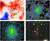 |
Fig. 2. Multiwavelength view of CL0238. The top row shows the relatively large-scale ACT (90 GHz; smoothed with 30 arcsec) and eROSITA images of the cluster in the 0.3–2.3 keV energy band. The bottom row shows the Chandra image ([0.8–4.0] keV) and the pseudo-color DESI Legacy Imaging Surveys image in the zrg (RGB) filters. The red galaxies at the image center are distributed along the vertical direction, and in all other images, the cluster is clearly elongated in the same direction. The observed elongation is an indication of the perturbed dynamical state of the cluster. The circle has a radius of 3.9 arcmin ≈R500, the green box has a side of 3 arcmin, the central cross marks the cluster center as defined for presentation purposes. |
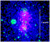 |
Fig. 3. Central part of CL0238 at the optical and X-ray wavelengths. The image shows a combination of X-ray data (magenta-blue) and optical r-band DESI image (green). A few bright galaxies that most likely belong to the cluster are highlighted with circles. Notably, a compact group of four visually clustered galaxies in the north lies just north beyond the brightest X-ray region of the cluster. |
4.2. Global observables and mass estimates of CL0238
To gain further insight into the cluster dynamical state, we analyzed Chandra and eROSITA spectra extracted from a circular region with a radius of R500 = 3.9 arcmin ≈1.3 Mpc (Fig. 2). For the background region, we used a ring with R500 < R < 2R500. The resulting eROSITA and Chandra spectra are shown in Fig. 4. We fit the spectra assuming an absorbed APEC (Smith et al. 2001) model (phabs*apec) with the following model parameters: The hydrogen column density was set to the value of NH = 1.2 ⋅ 1021 cm−2 (based on the approach of Willingale et al. 2013), the metal abundance was set to 0.3 solar, and the redshift was set to z = 0.42. The simultaneous fit of eROSITA and Chandra spectra resulted in the best-fit temperature of T500 = (9.95 ± 0.79) keV. The rest-frame cluster luminosity in the [0.5, 2.0] keV band is L500 ≈ 7.9 ⋅ 1044 erg/s, and it is weakly sensitive to the exact value of R500.
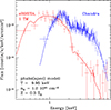 |
Fig. 4. eROSITA and Chandra spectra of CL0238 extracted from a circle with a radius of R500 = 3.9 arcmin. An annulus with R500 < R < 2R500 is used as the background region. Point sources are subtracted. The eROSITA spectrum is normalized per one (out of seven) eROSITA telescope modules. The best-fit absorbed APEC model obtained from the joint analysis of eROSITA+Chandra data is shown with solid curves. The blue and red curves correspond to the same spectral model convolved with the Chandra and eROSITA responses, respectively. |
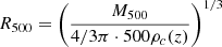
Using scaling relations from Vikhlinin et al. (2009) for the measured temperature and X-ray luminosity, we found the following estimates of the total mass: 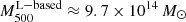 and
and 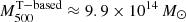 , respectively. We note here that given the ongoing merger, the cluster gas is likely to be heated by a shock wave, and our X-ray-based temperature, luminosity, and mass estimate might be biased high. Several studies evaluated the accuracy of various ways of estimating mass (for instance, Pinkney et al. 1996; ZuHone et al. 2009; Krause et al. 2012). The general agreement is that the accuracy of a mass estimation depends on the merger geometry, its phase, and the line-of-sight (l.o.s.) angle. Therefore, the above estimate is likely subject to systematic uncertainties, which might be reduced after a detailed modeling.
We conducted optical spectroscopic observations (see Sect. 2) of several galaxies, which are likely to be CL0238 cluster members, and with these data in hand, we derived a rough estimate of the velocity dispersion of the cluster and used it as an additional mass proxy. Based on spectroscopic redshifts available for five galaxies in the cluster (see Table 1 and Fig. 1), we estimated the average redshift ⟨z⟩ = 0.4191 and relative l.o.s. velocities Vlos of the galaxies as
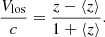 (1)
(1)
The cluster velocity dispersion can be estimated as
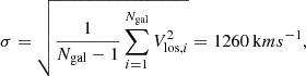 (2)
(2)
where Ngal = 5. Taken at face value, the derived velocity dispersion in excess of 1000 km s−1 also indicates a high cluster mass (e.g. Evrard et al. 2008), although the uncertainties are large. Even though all our estimates are subject to different biases due to the perturbed state of the cluster, they are all roughly consistent with each other and indicate a high cluster mass.
4.3. Signatures of a disrupted cool core?
The Chandra X-ray images of CL0238 show that the cluster can be visually divided into two bright areas to the north and south, and a dip in between. We extracted spectra from these three regions (shown as circles of different colors in the top left panel of Fig. 5) and estimated the gas temperature. The northern and southern regions have a temperature of T = 10 ± 2 keV, and the region in the middle is colder, T = 7.9 ± 1.4 keV. The uncertainties on derived temperatures are large, and therefore, the evidence for the colder region is marginal. To additionally test for the presence of colder gas, we used the eROSITA image in the soft energy band 0.3–0.7 keV (right panel of Fig. 5). A tentative excess of soft photons is seen at the cluster center. The region with the sightly enhanced surface brightness in the 0.3–0.7 keV band is marked with the black ellipse. This ellipse overlaps with the middle region with colder gas as measured using Chandra data. Despite these hints, the evidence for the cool gas is marginal, and more data are needed to confirm it.
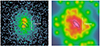 |
Fig. 5. Zoom into the CL0238 core. Left: Chandra X-ray image with the three circular regions (≈19 arcsec in diameter) that we used to analyze the projected spectra. The best-fitting temperatures are 10.2 ± 2 keV for the bright region to the north (red circle) and 10 ± 1.9 keV for the bright region to the south (blue circle). The temperature measured for the central region (green circle) is slightly lower 7.9 ± 1.4 keV, although the uncertainties of all three measurements are large and the assumption that the temperatures are consistent cannot be rejected. Right: eROSITA image in the [0.3 − 0.7] keV energy range, where the ACIS efficiency drops significantly (see Fig. 6.8 in https://cxc.harvard.edu/proposer/POG/html/chap6.html#tthsEc6.2). The region with the slightly enhanced surface brightness is marked with the dashed ellipse. This ellipse lies just in between the north and south regions with a high X-ray surface brightness in the Chandra image, which corroborates the presence of colder gas in the region. We speculate that this gas might be stripped from the core of the merging subclusters. |
Cold gas at a cluster center is often observed for cool-core clusters, in which the peak of the X-ray surface brightness and the lowest gas temperatures are centered at the brightest elliptical galaxy. This is clearly not the case for CL0238. The brightest galaxies in the most prominent northern group are shifted from the peak of the X-ray emission, and the cool gas (if any) is even farther away from these galaxies. From a simple β-model approximation6 of the cluster radial profile and an APEC spectral model, we estimated the central electron density in the cluster core, ne ≈ 2 × 10⁻³ cm−3. Adopting the cooling function of Sutherland & Dopita (1993) with the abundance of heavy elements of one-third solar, we obtained the cooling time of the gas as ∼1.6 × 10¹⁰ yr, which is almost twice longer than the Hubble time at z = 0.42.
The derived long cooling time, combined with the lack of bright optical galaxies in this region and the absence of a prominent peak in X-rays, suggests that the softer emission is not a canonical cool core. Instead, it could be stripped gas from a cool core that one of the merging subhalos possessed before the merger.
5. Merger geometry and velocity
The measured velocities of five galaxies (see Fig. 1) corroborate the merger scenario. We tentatively assumed that the two galaxies in the north (with z ≈ 0.42) belong to one subcluster and that the two in the south (with z ≈ 0.41) belong to the second subcluster. Yet another galaxy to the south from the core has a redshift closer to the redshifts of two galaxies in the northern clump. The four possible configurations of the two merging groups are sketched in the left panel of Fig. 6. In our favored scenario, the northern clump has already passed the pericenter, that is, the cluster is in the post-merger state. Combined with the higher recession velocity of this clump, the top left configuration appears to be the most plausible configuration.
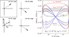 |
Fig. 6. Constraints on the merger angle θ relative to the l.o.s. assuming a head-on collision of two subhalos. Left: Four possible configurations with the same angle θ and projected distance dproj between subhalos. Only one of these configurations (marked with a box) fits the scenario discussed here. Namely, (i) the northern subhalo recedes from us with a higher velocity than the southern one and (ii) this is a post-merger phase. Right: Expected and observed velocity differences for two pairs of galaxies that are considered as proxies for the subhalo positions and velocities. These two pairs have ΔV and dproj of 2060 km s−1 & 220 kpc and 3200 km s−1 & 142 kpc, respectively. The black and red curves (solid and dashed) show for each pair the 3D distance between the galaxies (d = dproj/sin θ) and the corresponding value of Vrel(d) (as given by Eq. (3)). The three close pairs of blue curves show the expected l.o.s. velocity differences f × (2Φ(d))1/2cos θ, where f is the suppression factor discussed in the text. The curves are shown for f = 1, 0.7, 0.5, where 0.7 is the fiducial value. The almost symmetric butterfly pattern of the blue curves reflects the different geometries shown in the left panel. Only the top left part of the plot corresponds to the merger scenario discussed here. The thin gold lines show the changes in these curves due to the Hubble expansion, which might be important only in the unlikely case of a merger axis that is almost perfectly aligned with the line of sight. The two horizontal brown lines (solid and dashed) show the observed l.o.s. velocity difference for each pair. |
Given the sparseness of the redshift data, we resorted to the simplest estimates of the merger geometry that can relate two observables: the projected distance separation dproj, and the l.o.s. velocity difference Vlos. Namely, we considered a test particle that falls in radially from infinity into a halo with a given mass M and a Navarro-Frenk-White profile (see e.g., Dawson 2013; Wittman 2019, for more elaborate analytical or numerical models).
In this model, the relative velocity Vrel of the test particle at separation d from the core of the main cluster is
 (3)
(3)
For d → 0, Vrel is the halo escape velocity Vesc, which for c200 = 4 is equal to  , that is, ≈5500 km s−1 for M200 = 1.4 × 10¹⁵ M⊙. In numerical simulations, the infall velocities of massive halos do not reach values ≈Vesc, but are systematically lower even when a head-on merger is considered (see, e.g., Hayashi & White 2006; Farrar & Rosen 2007; Springel & Farrar 2007, for the discussion of the Bullet cluster case). The values predicted by Eq. (3) (with d not very close to zero) likely also exceed real velocities. For instance, Łokas (2023) recently examined ten merging clusters in the IllustrisTNG300 simulation and derived the distances of the closest approach and relative velocities. For these mergers, the velocities found in simulations Vsim are at the level of ∼0.6Vrel (using Eq. (3) for the mass of the main halo and the separation from their Table 1, and setting c200 to 4 for all halos). However, for the two most massive mergers, the agreement is better (Vsim ∼ 0.7 and 0.8 Vrel for these two cases). The truncation of the NFW mass distribution at R200 (as in the model of Dawson 2013) reduces the value of Vesc by a factor
  . The further simplifying assumption that the two halos maintain their shapes reduces Vesc to 0.6 − 0.7 of
  , provided that the main halo and the subhalo have the same masses/sizes, since in this case, the velocity is set not by the depth of the main halo potential at d = 0, but is the mass-weighted mean value. Given the above considerations, we assumed that the velocities predicted by Eq. (3) are likely overestimated (similarly to Vesc for d = 0) and have to be scaled down by a factor in the range of ∼0.5–0.7-1 when compared with observations.
We adopted the mass of our system as M200 = 1.4 ⋅ 1015 M⊙ as derived from the M500 estimate obtained in Sect. 4.1, and the mass-concentration relation from Diemer & Joyce (2019). For each angle θ between the merger axis and our l.o.s., from the observed distance dproj between merging subhalos and the measured radial velocity difference, we calculated the separation d between the merging clusters in 3D and the total relative velocity using Eq. (3) (see Fig. 6).
One subhalo is most plausibly associated with four (visually) clustered galaxies to the north (see Fig. 1). The position of the second subhalo is uncertain. We tentatively associate it with a galaxy located within the bright X-ray area to the south, about 40.3 arcsec away in projection from the galaxy to the north. The l.o.s. velocity difference between these two galaxies is Vlos, obs = cΔz/(1 + zcl) = 2060 km s−1, and the projected distance is dproj = 40.3 arcsec = 220 kpc. We also considered another galaxy with z = 0.4104 as a possible candidate for the second subhalo. For this case, the observed velocity difference is Vlos, obs = 3200 km s−1 and dproj = 25.6 arcsec = 142 kpc in projection.
Fig. 6 illustrates the constraints on the possible viewing angle. Four possible merger configurations with the same angle θ and projected distance dproj between the subhalos are sketched in the left panel. The right panel shows the expected l.o.s. velocity difference for a pair of subhalos with a given θ and projected distance dproj. Namely, we calculated d = dproj/sin θ and used the scaled version of Eq. (3) to estimate the 3D velocity of merging subclusters, that is, ΔV = f × [2|ΦNFW(d)|]1/2 assuming that M200 = 1.4 × 10¹⁵ M⊙ and c200 = 4. The expected l.o.s. velocity difference is then Vlos, model = ΔV cos θ, which can be compared with observations. To this end, we assumed that the two pairs of galaxies shown in Fig. 1 can be used as two independent proxies for merging subhalos, and we plot corresponding Vlos, model curves for these two pairs for the entire range of θ and three values of f. Since projected separations are comparable (and small) for both pairs, the expected Vlos, model curves are also very similar (see the blue lines in Fig. 6). Guided by the Chandra and optical images (Fig. 3), we assumed that the system is in a post-merger phase, that is, the northern group (marked N) is moving away from the other group (more to the south from the cluster centroid). Coupled with the higher recession velocity of group N, only the configuration shown in the upper left corners of both panels is qualitatively consistent with our scenario. We then compared the predicted values of Vlos, model with the observed velocity differences Vlos, obs for each pair. The latter values are shown in Fig. 6 with two horizontal brownlines. Ideally, the blue curves might intersect these lines at the same value of θ. Not surprisingly, this does not happen in Fig. 6. It would indeed be a remarkable coincidence because this comparison is based on the (almost) randomly selected galaxies and other uncertainties in the definition of the model. A more reasonable approach is to identify a range of angles that is probably not suitable for CL0238. For θ close to 90 degrees, that is, a merger on the plane of the sky, the expected l.o.s. velocities are obviously low. For f = 0.7, for instance, the values of θ ≳ 60 − 70 deg are implausible. Smaller angles cannot be excluded, except for very small angles, that is, when the merger direction is almost along the line of sight. In this case, the physical separation is too large and the N and S groups will not interact physically, which contradicts our assumption. The remaining additional argument is simply the probability of observing a randomly oriented system at a given angle θ. This probability is ∝sin θ, and it therefore favors large angles. All these indirect arguments suggest that the merger is at some large angle that is not yet excluded by the high values of Vlos, obs. For the estimates, we set θ ∼ 45 deg so that the velocities in the plane of the sky were on the same order as the observed l.o.s. velocities. Future observations can help us to refine the constraints on this angle.
With these assumptions, the projected distance of ∼200 kpc translates into a 3D separation of ∼300 kpc, which means that the two subhalos are very close to each other. Using Eq. (3) and adopting f = 0.7, we estimated a relative velocity of ∼3500 km s−1, and the estimated time for crossing 300 kpc is ≲0.1 Gyr. This emphasizes the short lifetime of the observed merger phase in CL0238.
As discussed above, both X-ray and optical mass proxies can be biased high for merging clusters. A global observable such as the integrated Comptonization parameter Y (or the equivalent X-ray mass proxy YX) has been shown to serve as a more robust mass proxy through the entire duration of a merger event (e.g., Kravtsov et al. 2006; Poole et al. 2007; Wik et al. 2008, among others). To this end, we note that from the joint analysis of Planck and ROSAT data, Tarrio et al. (2019) estimated the CL0238 mass to be  . Converting this value into M200 as ≈1.4 × M500 ≈ 9 × 10¹⁴ M⊙ reduces the characteristic velocities by ∼15%. This would further shrink the range of plausible angles (and introduce a greater difference for the pair of galaxies with the l.o.s. velocity difference of 3120 km s−1).
6. Discussion
6.1. Comparison of CL0238 with MACS0416 and the Bullet cluster
We now proceed with a qualitative comparison of CL0238 with two other prominent merger systems: MACS J0416.1–2403 and the Bullet cluster.
MACS J0416.1–2403 is a merging cluster at z = 0.396. Similarly to CL0238, it is characterized by a high mass and X-ray temperature (kT ≈ 10 keV, M ≈ 1015 M⊙; Jauzac et al. (2015), Ogrean et al. (2015)), an elongated mass distribution, and a double-peaked X-ray image (Mann & Ebeling 2012). Most recent studies favored a pre-collision scenario (Ogrean et al. 2015; Balestra et al. 2016; Bonamigo et al. 2017) for MACS J0416.1–2403 and confirmed that there is no significant offset between the dark matter and the stellar/gas components (see also Jauzac et al. 2015; Diego et al. 2015, for alternative scenarios).
The Bullet cluster (1E 0657-56) at z = 0.296 is a canonical example of a post-merger cluster. It exhibits spatial offsets between its dark matter and baryonic density peaks derived from the gravitational lensing maps and the gas distribution (see, e.g., Markevitch et al. 2004; Clowe et al. 2006; Paraficz et al. 2016). It is also a very massive M ∼ 1015 M⊙ and hot cluster with a spectacular bullet-like X-ray core and a leading bow shock.
The question now is how different CL0238 is from MACS J0416.1–2403 and the Bullet. In Fig. 7 we show X-ray and optical images of these three clusters (all rotated to align the apparent elongation along the vertical axis). The left and right panels show the Chandra X-ray images and the DESI r-band images (showing the distribution of galaxies), respectively. To obtain the images in the middle panels, we first approximated the individual X-ray images with a β-model plus a constant background. Then, from each Chandra image, we subtracted the corresponding model and divided by the model (i.e., (image-model)/model). Very prominent deviations from the beta models are seen for all three clusters. For MACS0416, the triangular-shaped features point toward each other, which indicates a pre-core-passage phase.
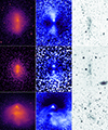 |
Fig. 7. Three stages of the merger illustrated by X-ray and optical images of three massive clusters. From top to bottom: Before the pericenter passage (MACS J0416), shortly after pericenter passage (CL0238), and slightly later (Bullet). The left panels show Chandra X-ray images. The panels in the middle present the residuals after the best-fitting symmetric model of a cluster+background was subtracted from the X-ray image and after dividing by the model (i.e., |

The Bullet cluster also has two prominent substructures, but unlike the MACS0416 cluster, the triangle now points away from the second substructure with a rather complicated morphology. This configuration is robustly identified as a post-merger cluster. It is thought that in the Bullet cluster, the merger is nearly in the plane of the sky. The estimates of the relative velocities of its two subclusters come predominantly from the gas density, temperature, and pressure jumps at the prominent bow shock ahead of one of the subclusters. The corresponding estimates of the bow shock Mach number vary between ≈2.5 and ≈3 (Markevitch et al. 2002, 2004; Markevitch 2006; Randall et al. 2008; Di Mascolo et al. 2019), implying a shock velocity ≳4000 km s−1. However, the velocity of the bow shock can be higher or lower than that of the galaxies (e.g. Springel & Farrar 2007; Zhang et al. 2019a).
CL0238 (middle row) also features two peaks in the X-ray image. Unlike MACS0416, however, the optical galaxies (northern clump) are observed at a larger distance from the center than the nearest X-ray peak. Assuming that ram pressure acting on the gas causes the displacement of the X-ray peaks, we conclude that CL0238 is in the post-pericenter-passage phase and that the gas has been strongly shifted from the potential wells traced by galaxies. This suggests a closer analogy to the Bullet cluster. However, the apparent (and physical) distance between the peaks is significantly smaller than in the Bullet cluster. We therefore propose that CL0238 corresponds to some intermediate phase between the MACS0416 and the Bullet clusters.
Moderately strong bow shocks that are expected in the scenario of a close-to-pericenter merger ahead of the subhalos that manage to retain some gas (see Springel & Farrar 2007; Zhang et al. 2019a; ZuHone et al. 2018) are not convincingly identified in the relatively shallow X-ray image of CL0238, although the bow to the south from the blobs is an interesting candidate. Another possibility is that the X-ray emission from the northern blob is dominated by shocked gas. With deeper X-ray observations, we might not only detect a bow shock, but also estimate the merger velocity, assuming that the infalling subcluster velocity is close to the shock velocity. The shock velocity Vshock is in turn related to the downstream temperature via
![Mathematical equation: $$ \begin{aligned} kT=\frac{3}{16}\mu m_p V_{\rm shock}^2\approx 10 \left[\frac{V_{\rm shock}}{2.9\times 10^{3}\,\mathrm{km\,s}^{-1}}\right]^2 \,\mathrm{keV}, \end{aligned} $$](/articles/aa/full_html/2025/01/aa52212-24/aa52212-24-eq12.gif) (4)
(4)
for the gas with the adiabatic index of 5/3 and a low initial temperature, that is, the case of a strong shock with a Mach number M ≫ 1. A lower shock velocity will be needed when the gas upstream is hot. For example, for the initial temperature of kT = 6 keV, a shock velocity of ∼2100 km s−1 is sufficient to have ∼10 keV gas downstream. For the high temperatures and low densities characteristic of CL0238, the electron-ion temperature equilibration time due to Coulomb collisions can be substantial, and for a given shock velocity, the electron temperature immediately downstream of the shock might be lower, similar to the Bullet cluster (e.g. Mickaelian et al. 2006). Useful constraints can be obtained when the temperature, density, and pressure jumps can be measured simultaneously using X-ray and SZ spatially resolved data (see Di Mascolo et al. 2019, for the Bullet cluster analysis).
6.2. Lensing
It is well established that massive systems such as galaxy clusters can act as gravitational lenses and reveal the properties of high-redshift objects that would otherwise be undetectable with current telescopes (see the recent review by Natarajan et al. (2024)). Cluster lenses are now routinely used to study the most distant galaxies (for example, Di Teodoro et al. 2018; Wang et al. 2023), to detect single stars at a cosmological distance (Kaurov et al. 2019, and others works), to investigate supernova explosions (for instance, Kelly et al. 2023; Baklanov et al. 2021), and for cosmography with time-delay analyses (Grillo et al. 2024, among many others).
MACS J0416.1–2403 is one of the Hubble Frontier Fields clusters and is characterized by a high lensing efficiency (Ogrean et al. 2015). The high lensing efficiency of MACS J0416 is thought to be due to several factors (for details, see Ogrean et al. 2015). First, the high cluster ellipticity increases the ratio of the caustic area in the source plane relative to the critical area, thus generating more multiple images of background sources for the same critical area (Ogrean et al. 2015; Meneghetti et al. 2007). Second, ongoing mergers have larger high-magnification regions than noninteracting clusters, and the total number of multiple images increases with lower separation between merging subhalos, especially when two merging clumps are separated by a distance ≤300 kpc/h (Ogrean et al. 2015; Torri et al. 2004; Redlich et al. 2012). Another factor driving the lensing efficiency could be the number of substructures (galaxies) in halos, especially in their central regions. The overall mass profile becomes shallower and provides higher magnifications. Meneghetti et al. (2007) found that ellipticity and substructures influence the lensing efficiency almost to the same extent on average. However, the authors noted that the effect of substructures is less important in highly asymmetric lenses.
As mentioned above, the properties of MACS J0416 are similar to those of CL0238 in many respects. They are located at similar redshifts and have comparable hot gas temperatures and total masses, and both clusters are highly elongated as traced by X-ray and optical images. We therefore suggest that CL0238 is an interesting target for deeper optical plus spectroscopic observations and a gravitational lensing analysis. Potentially, the lensing efficiency of CL0238 is as high as for MACS J0416, and CL0238 may provide a number of magnified high-redshift sources.
6.3. SZ, kSZ, and polarization
A combination of X-ray and Sunyaev-Zeldovich (SZ) effect data can be used to infer the gas temperature Sunyaev & Zeldovich (1980a); see Section 4 in Churazov et al. (2021) or Mroczkowski et al. (2019) for a recent review). To this end, we used the parameters derived from X-ray images and spectra. Namely, the approximation of the radial profile with the simple β-model yields rc = 0.47′, β = 0.69, and a central electron density ne = 2 × 10⁻³ cm−3. For kT = 10 keV, the expected mean value of the Compton y = 2.5 × 10⁻⁶ within a 10′ (radius) circle centered at CL0238. This value agrees well with the mean y extracted from the Planck data, yPl = 2.4 × 10⁻⁶, for a similar region. For this exercise, the PR2 y map was used (Planck Collaboration XXII 2016).
Given the estimated parameters of the merger, a substantial contribution of the kinematic SZ signal (due to the high l.o.s. velocity) (Sunyaev & Zeldovich 1980b) and polarization in the microwave band (due to the high transverse velocity) are expected (Sunyaev & Zeldovich 1980b; Sazonov & Sunyaev 1999; Mroczkowski et al. 2019, for a review). In particular, Fig. 8 shows the estimated tSZ and kSZ signals (in MJy/sr) for the cluster core. The same β model was used to estimate τT and y for the cluster core. For kSZ, the amplitudes for ±1500 km s−1 are shown.
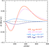 |
Fig. 8. Expected SZ signals for the line of sight going through the cluster center. For tSZ (red curve), τT = 1.9 × 10⁻³ and kT = 10 keV were assumed. The kSZ signal (two blue curves) corresponds to a velocity of ±1500 km s−1 and the same τT as for the tSZ. For completeness, the magenta line shows the tSZ signal with relativistic corrections for 10 keV electrons. |
For merger angles of ∼45 deg, similar velocities in the sky plane are expected. In this case, a polarized SZ signal associated with the sub-clusters motion relative to the CMB frame is expected. Its magnitude (Sunyaev & Zeldovich 1980b) is  for v⊥ ∼ 1500 km s−1. Moreover, given the highly dynamical nature of the interaction, gyrotropic pressure anisotropies are expected to be driven in large volumes of the weakly collisional ICM plasma, especially behind the shock fronts and in the turbulent wakes of massive substructures (Komarov et al. 2016; Khabibullin et al. 2018). As a result, sensitive high-resolution polarimetric SZ observations of CL0238 might provide insights into the actual collisionality and turbulence properties of the ICM plasma.
The caveat for the above estimates is the uncertainty of the gas velocities. For a dissociative merger, the gas velocity can be substantially lower than the velocities of galaxies and/or dark matter. However, if the halos are able to retain the gas after the pericenter passage, the gas can move even faster than the parent halo (a slingshot effect, see, e.g. Springel & Farrar 2007; Zhang et al. 2019a; Lyskova et al. 2019; Sheardown et al. 2019). By combining the optical, X-ray, and kSZ data, we can reveal the true geometry of the merger and the merger phase. To this end, additional spectroscopic redshifts and X-ray data (including XRISM) would be especially useful in combination with spatially resolved SZ data. For the latter, a resolution of the two cores, which are separated by ≈30″, would require instruments with a sufficiently high angular resolution, for example, ALMA, MUSTANG-2, or NIKA.
6.4. Radio properties of CL0238
Given the high velocity of the merger, it is plausible that CL0238 might feature nonthermal radio emission (for a review, see van Weeren et al. 2019), associated with shocks and/or turbulence generated by the ongoing merger. The detection of the former would help us to improve the geometrical model of the merger, while the latter might serve as a tracer for the merger state.
In Figure 9 we show the RACS (Rapid ASKAP Continuum Survey McConnell et al. 2020) and TGSS (TIFR GMRT Sky Survey; Intema et al. 2017) radio images of the cluster at 887 MHz and 150 MHz, respectively. The most prominent sources are labeled. Source A is located to the north of the cluster. It has a compact core, but there is also a fainter radio emission that apparently extends in the north-south direction. Additionally, there is a hint that source A and source B are connected via a fainter emission (at the 2σ level).
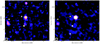 |
Fig. 9. Radio emission from the cluster CL0238 at 887 MHz (left) and 150 MHz (right). The 887 MHz and 150 MHz images are from the RACS and TGSS surveys. In both maps, the radio contour levels are drawn at [1, 2, 4, 8, …]×3.0σrms. The noise level in the ASKAP and GMRT images is 170 μJy beam−1 and 1.6 mJy beam−1, respectively. |
From the RACS map, we measured that source A has an extent of about 650 kpc. It has a flux density of 19 ± 2 mJy, 750 ± 150 mJy, and 1.6 ± 0.3 Jy at 887, 150, and 88 MHz (using the GLEAM survey), respectively. This indicates that source A has a very steep radio spectral index7 of  . An optical image at the position of source A is shown in Figure 10. We cannot unambiguously identify the optical counterpart that coincides with the peak radio flux of source A. The spectral index distribution across it (right panel of Figure 10) is inconsistent with that of a head-tail radio galaxy, where we expect a flat spectral index in the core region (−0.5 to −0.7) and gradual spectral steepening across its tails. Moreover, the extremely steep spectral index rules out an identification as a radio-loud AGN within the cluster, which typically has a spectral index of −0.7.
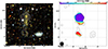 |
Fig. 10. Left: Optical image overlaid with the RACS radio contours. Right: Spectral index map created between 150 and 887 MHz. The Stokes I 887 MHz radio contours are drawn at [1, 2, 4, 8, …]×3.0σrms. |
Due to its very steep spectral index, location, and small size, source A could be a radio phoenix. These sources are thought to trace fossil plasma from radio galaxies that were reenergized by adiabatic compression after the passage of a shock wave in the ICM (e.g., Enßlin & Brüggen 2002; Mandal et al. 2019; Zhang et al. 2019b). However, due to the poor resolution and sensitivity of the existing radio data, its nature remains uncertain.
Source B has an optical counterpart, but its redshift is unknown. To the east of the cluster is an arc-like diffuse extended source, source C (see Figure 9 left panel). It has an extent of about 640 kpc. The source is partially detected in the 150 MHz TGSS survey.
Given the available data, we conclude that there are indications of a displacement and extended features in the data, but high-sensitivity data, especially at low frequencies, are needed to draw firm conclusions.
7. Conclusions
Current X-ray, SZ, and optical observations show that CL0238 is a massive (M200 ∼ 1015 M⊙) galaxy cluster that is undergoing a merger. At X-ray and optical wavelengths, the cluster is elongated in the north-south direction, which presumably is the axis of the merger. The peaks in the X-ray and galaxy number density distributions are displaced, which indicates that the cluster is caught soon after the first core passage. The mean gas temperature is ∼10 keV. There are indications of cooler gas between the two X-ray peaks, but more data are needed to confirm its presence. An approximate modeling of the merger geometry (based on a few available spectroscopic redshifts and the spatial distribution of galaxies) suggests that the merger axis makes a substantial angle to the line of sight, and therefore, the true 3D separation of the likely merging subcluster cores is not much larger than their separation in the plane of the sky, ∼200 kpc. Our approximate modeling also implies that the pericenter passage occurred ≲0.1 Gyr ago.
We compared CL0238 with the two well-known clusters MACS0416 and the Bullet, and we concluded that CL0238 corresponds to an intermediate phase between the pre-merging MACS0416 cluster and the post-merger Bullet cluster. The high mass, high elongation, and intermediate redshift of CL0238 make this cluster an interesting target for a gravitational lensing analysis. CL0238 is similar in many properties to MACS0416, which is known for its high lensing efficiency, and it might be expected that with deeper optical observations, a considerable number of high-redshift sources that are magnified by the cluster lens CL0238 will be discovered.
Data availability
A copy of the reduced images and spectra is available at the CDS via anonymous ftp to cdsarc.cds.unistra.fr (130.79.128.5) or via https://cdsarc.cds.unistra.fr/viz-bin/cat/J/A+A/693/A55
Throughout the paper, the cluster mass is defined as MΔ = 4/3πRΔ3Δρc, where RΔ is the radius enclosing an overdensity Δ with respect to the critical density ρc of the Universe at a given redshift.
To convert M200 = 6 × 10¹⁴ M⊙ from Wen et al. (2012) into M500, we assumed the mass-concentration relation from Diemer & Joyce (2019) and a Navarro-Frenk-White cluster density profile.
RTT-150 spectra were processed using the IRAF package (https://iraf-community.github.io), and redshifts measurements were made by using the software developed by Irek Khamitov and Rodion Burenin.
There is no X-ray peak at this position. Rather, the defined center reflects the X-ray surface brightness distribution on scales of 1 − 3 arcmin.
 , where ρc is the critical density of the Universe.
With β = 0.69, rc = 0.47 arcmin and the cluster center at RA = 02:38:20.8, Dec = +20:05:56.
We define the radio spectral index, α, so that Sν ∝ να, where S is the flux density at frequency ν.
Acknowledgments
We are grateful to the referees for their comments. We also thank Klaus Dolag for helpful discussions. The authors are grateful to TUBITAK, IKI, KFU, and the Tatarstan Academy of Sciences for partial support in the use of RTT-150 (the Russian-Turkish 1.5-m telescope in Antalya). The work of IFB, IMK, MAG, MVS, RIG, NAS was supported by the subsidy from the Ministry of Science and Higher Education of the Russian Federation FZSM-2023-0015, allocated to Kazan Federal University to fulfill the state assignment in the field of scientific activity. IK acknowledges support by the COMPLEX project from the European Research Council (ERC) under the European Union’s Horizon 2020 research and innovation program grant agreement ERC-2019-AdG 882679. WF, CJ, and RK acknowledge support from the Smithsonian Institution, the Chandra High Resolution Camera Project through NASA contract NAS8-0306, NASA Grant 80NSSC19K0116 and Chandra Grant GO1-22132X. In this work, observations with the eROSITA telescope onboard SRG space observatory were used. The SRG observatory was built by Roskosmos in the interests of the Russian Academy of Sciences represented by its Space Research Institute (IKI) in the framework of the Russian Federal Space Program, with the participation of the Deutsches Zentrum für Luft- und Raumfahrt (DLR). The eROSITA X-ray telescope was built by a consortium of German Institutes led by MPE, and supported by DLR. The SRG spacecraft was designed, built, launched, and operated by the Lavochkin Association and its subcontractors. The science data are downlinked via the Deep Space Network Antennae in Bear Lakes, Ussurijsk, and Baikonur, funded by Roskosmos. The eROSITA data used in this work were converted to calibrated event lists using the eSASS software system developed by the German eROSITA Consortium and analysed using proprietary data reduction software developed by the Russian eROSITA Consortium. This work is based on publicly available optical data from the DESI Legacy Imaging Surveys. The Legacy Surveys consist of three individual and complementary projects: the Dark Energy Camera Legacy Survey (DECaLS; Proposal ID #2014B-0404; PIs: David Schlegel and Arjun Dey), the Beijing-Arizona Sky Survey (BASS; NOAO Prop. ID #2015A-0801; PIs: Zhou Xu and Xiaohui Fan), and the Mayall z-band Legacy Survey (MzLS; Prop. ID #2016A-0453; PI: Arjun Dey). DECaLS, BASS and MzLS together include data obtained, respectively, at the Blanco telescope, Cerro Tololo Inter-American Observatory, NSF’s NOIRLab; the Bok telescope, Steward Observatory, University of Arizona; and the Mayall telescope, Kitt Peak National Observatory, NOIRLab. Pipeline processing and analyses of the data were supported by NOIRLab and the Lawrence Berkeley National Laboratory (LBNL). The Legacy Surveys project is honored to be permitted to conduct astronomical research on Iolkam Du’ag (Kitt Peak), a mountain with particular significance to the Tohono O’odham Nation. NOIRLab is operated by the Association of Universities for Research in Astronomy (AURA) under a cooperative agreement with the National Science Foundation. LBNL is managed by the Regents of the University of California under contract to the U.S. Department of Energy. This project used data obtained with the Dark Energy Camera (DECam), which was constructed by the Dark Energy Survey (DES) collaboration. Funding for the DES Projects has been provided by the U.S. Department of Energy, the U.S. National Science Foundation, the Ministry of Science and Education of Spain, the Science and Technology Facilities Council of the United Kingdom, the Higher Education Funding Council for England, the National Center for Supercomputing Applications at the University of Illinois at Urbana-Champaign, the Kavli Institute of Cosmological Physics at the University of Chicago, Center for Cosmology and Astro-Particle Physics at the Ohio State University, the Mitchell Institute for Fundamental Physics and Astronomy at Texas A&M University, Financiadora de Estudos e Projetos, Fundacao Carlos Chagas Filho de Amparo, Financiadora de Estudos e Projetos, Fundacao Carlos Chagas Filho de Amparo a Pesquisa do Estado do Rio de Janeiro, Conselho Nacional de Desenvolvimento Cientifico e Tecnologico and the Ministerio da Ciencia, Tecnologia e Inovacao, the Deutsche Forschungsgemeinschaft and the Collaborating Institutions in the Dark Energy Survey. The Collaborating Institutions are Argonne National Laboratory, the University of California at Santa Cruz, the University of Cambridge, Centro de Investigaciones Energeticas, Medioambientales y Tecnologicas-Madrid, the University of Chicago, University College London, the DES-Brazil Consortium, the University of Edinburgh, the Eidgenossische Technische Hochschule (ETH) Zurich, Fermi National Accelerator Laboratory, the University of Illinois at Urbana-Champaign, the Institut de Ciencies de l’Espai (IEEC/CSIC), the Institut de Fisica d’Altes Energies, Lawrence Berkeley National Laboratory, the Ludwig Maximilians Universitat Munchen and the associated Excellence Cluster Universe, the University of Michigan, NSF’s NOIRLab, the University of Nottingham, the Ohio State University, the University of Pennsylvania, the University of Portsmouth, SLAC National Accelerator Laboratory, Stanford University, the University of Sussex, and Texas A&M University. BASS is a key project of the Telescope Access Program (TAP), which has been funded by the National Astronomical Observatories of China, the Chinese Academy of Sciences (the Strategic Priority Research Program “The Emergence of Cosmological Structures” Grant # XDB09000000), and the Special Fund for Astronomy from the Ministry of Finance. The BASS is also supported by the External Cooperation Program of Chinese Academy of Sciences (Grant # 114A11KYSB20160057), and Chinese National Natural Science Foundation (Grant # 12120101003, # 11433005). The Legacy Survey team makes use of data products from the Near-Earth Object Wide-field Infrared Survey Explorer (NEOWISE), which is a project of the Jet Propulsion Laboratory/California Institute of Technology. NEOWISE is funded by the National Aeronautics and Space Administration. The Legacy Surveys imaging of the DESI footprint is supported by the Director, Office of Science, Office of High Energy Physics of the U.S. Department of Energy under Contract No. DE-AC02-05CH1123, by the National Energy Research Scientific Computing Center, a DOE Office of Science User Facility under the same contract; and by the U.S. National Science Foundation, Division of Astronomical Sciences under Contract No. AST-0950945 to NOAO. This scientific work uses Rapid ASKAP Continuum Survey (RACS) data obtained from Inyarrimanha Ilgari Bundara/the Murchison Radio-astronomy Observatory. We acknowledge the Wajarri Yamaji People as the Traditional Owners and native title holders of the Observatory site. CSIRO’s ASKAP radio telescope is part of the Australia Telescope National Facility (https://ror.org/05qajvd42). Operation of ASKAP is funded by the Australian Government with support from the National Collaborative Research Infrastructure Strategy. ASKAP uses the resources of the Pawsey Supercomputing Research Centre. Establishment of ASKAP, Inyarrimanha Ilgari Bundara, the CSIRO Murchison Radio-astronomy Observatory and the Pawsey Supercomputing Research Centre are initiatives of the Australian Government, with support from the Government of Western Australia and the Science and Industry Endowment Fund. This paper includes archived data obtained through the CSIRO ASKAP Science Data Archive, CASDA (https://data.csiro.au).
References
- Adhikari, S., Banerjee, A., Boddy, K. K., et al. 2022, Rev. Mod. Phys., submitted [arXiv:2207.10638] [Google Scholar]
- Afanasiev, V. L., & Moiseev, A. V. 2005, Astron. Lett., 31, 194 [NASA ADS] [CrossRef] [Google Scholar]
- Afanasiev, V. L., & Moiseev, A. V. 2011, Baltic Astron., 20, 363 [NASA ADS] [Google Scholar]
- Angrick, C., & Bartelmann, M. 2012, A&A, 538, A98 [NASA ADS] [CrossRef] [EDP Sciences] [Google Scholar]
- Baklanov, P., Lyskova, N., Blinnikov, S., & Nomoto, K. 2021, ApJ, 907, 35 [NASA ADS] [CrossRef] [Google Scholar]
- Balestra, I., Mercurio, A., Sartoris, B., et al. 2016, ApJS, 224, 33 [Google Scholar]
- Bonamigo, M., Grillo, C., Ettori, S., et al. 2017, ApJ, 842, 132 [NASA ADS] [CrossRef] [Google Scholar]
- Brunner, H., Boller, T., Coutinho, D., et al. 2018, SPIE Conf. Ser., 10699, 106995G [Google Scholar]
- Burenin, R. A., Zaznobin, I. A., Medvedev, P. S., et al. 2022, Astron. Lett., 48, 702 [NASA ADS] [CrossRef] [Google Scholar]
- Churazov, E., Khabibullin, I., Lyskova, N., Sunyaev, R., & Bykov, A. M. 2021, A&A, 651, A41 [NASA ADS] [CrossRef] [EDP Sciences] [Google Scholar]
- Clowe, D., Schneider, P., Aragón-Salamanca, A., et al. 2006, A&A, 451, 395 [NASA ADS] [CrossRef] [EDP Sciences] [Google Scholar]
- Dawson, W. A. 2013, ApJ, 772, 131 [NASA ADS] [CrossRef] [Google Scholar]
- Diego, J. M., Broadhurst, T., Molnar, S. M., Lam, D., & Lim, J. 2015, MNRAS, 447, 3130 [NASA ADS] [CrossRef] [Google Scholar]
- Diemer, B., & Joyce, M. 2019, ApJ, 871, 168 [NASA ADS] [CrossRef] [Google Scholar]
- Di Mascolo, L., Mroczkowski, T., Churazov, E., et al. 2019, A&A, 628, A100 [NASA ADS] [CrossRef] [EDP Sciences] [Google Scholar]
- Di Teodoro, E. M., Grillo, C., Fraternali, F., et al. 2018, MNRAS, 476, 804 [NASA ADS] [CrossRef] [Google Scholar]
- Enßlin, T. A., & Brüggen, M. 2002, MNRAS, 331, 1011 [Google Scholar]
- Evrard, A. E., Bialek, J., Busha, M., et al. 2008, ApJ, 672, 122 [Google Scholar]
- Farrar, G. R., & Rosen, R. A. 2007, Phys. Rev. Lett., 98, 171302 [NASA ADS] [CrossRef] [Google Scholar]
- Fischer, M. S., Durke, N.-H., Hollingshausen, K., et al. 2023, MNRAS, 523, 5915 [CrossRef] [Google Scholar]
- Grillo, C., Pagano, L., Rosati, P., & Suyu, S. H. 2024, A&A, 684, L23 [NASA ADS] [CrossRef] [EDP Sciences] [Google Scholar]
- Hayashi, E., & White, S. D. M. 2006, MNRAS, 370, L38 [NASA ADS] [CrossRef] [Google Scholar]
- Intema, H. T., Jagannathan, P., Mooley, K. P., & Frail, D. A. 2017, A&A, 598, A78 [NASA ADS] [CrossRef] [EDP Sciences] [Google Scholar]
- Jauzac, M., Jullo, E., Eckert, D., et al. 2015, MNRAS, 446, 4132 [Google Scholar]
- Kaurov, A. A., Dai, L., Venumadhav, T., Miralda-Escudé, J., & Frye, B. 2019, ApJ, 880, 58 [NASA ADS] [CrossRef] [Google Scholar]
- Kelly, P. L., Rodney, S., Treu, T., et al. 2023, ApJ, 948, 93 [NASA ADS] [CrossRef] [Google Scholar]
- Khabibullin, I., Komarov, S., Churazov, E., & Schekochihin, A. 2018, MNRAS, 474, 2389 [CrossRef] [Google Scholar]
- Khabibullin, I. I., Churazov, E. M., Bykov, A. M., Chugai, N. N., & Sunyaev, R. A. 2023, MNRAS, 521, 5536 [NASA ADS] [CrossRef] [Google Scholar]
- Khamitov, I. M., Bikmaev, I. F., Burenin, R. A., et al. 2020, Astron. Lett., 46, 1 [NASA ADS] [CrossRef] [Google Scholar]
- Komarov, S. V., Khabibullin, I. I., Churazov, E. M., & Schekochihin, A. A. 2016, MNRAS, 461, 2162 [NASA ADS] [CrossRef] [Google Scholar]
- Krause, E., Pierpaoli, E., Dolag, K., & Borgani, S. 2012, MNRAS, 419, 1766 [NASA ADS] [CrossRef] [Google Scholar]
- Kravtsov, A. V., & Borgani, S. 2012, ARA&A, 50, 353 [Google Scholar]
- Kravtsov, A. V., Vikhlinin, A., & Nagai, D. 2006, ApJ, 650, 128 [Google Scholar]
- Łokas, E. L. 2023, A&A, 673, A131 [NASA ADS] [CrossRef] [EDP Sciences] [Google Scholar]
- Lotz, J. M., Koekemoer, A., Coe, D., et al. 2017, ApJ, 837, 97 [Google Scholar]
- Lyskova, N., Churazov, E., Zhang, C., et al. 2019, MNRAS, 485, 2922 [Google Scholar]
- Mandal, S., Intema, H. T., Shimwell, T. W., et al. 2019, A&A, 622, A22 [NASA ADS] [CrossRef] [EDP Sciences] [Google Scholar]
- Mann, A. W., & Ebeling, H. 2012, MNRAS, 420, 2120 [NASA ADS] [CrossRef] [Google Scholar]
- Markevitch, M. 2006, ESA Spec. Publ., 604, 723 [NASA ADS] [Google Scholar]
- Markevitch, M., & Vikhlinin, A. 2007, Phys. Rep., 443, 1 [Google Scholar]
- Markevitch, M., Gonzalez, A. H., David, L., et al. 2002, ApJ, 567, L27 [Google Scholar]
- Markevitch, M., Gonzalez, A. H., Clowe, D., et al. 2004, ApJ, 606, 819 [NASA ADS] [CrossRef] [Google Scholar]
- McConnell, D., Hale, C. L., Lenc, E., et al. 2020, PASA, 37, e048 [Google Scholar]
- Meneghetti, M., Argazzi, R., Pace, F., et al. 2007, A&A, 461, 25 [NASA ADS] [CrossRef] [EDP Sciences] [Google Scholar]
- Mickaelian, A. M., Hovhannisyan, L. R., Engels, D., Hagen, H. J., & Voges, W. 2006, A&A, 449, 425 [NASA ADS] [CrossRef] [EDP Sciences] [Google Scholar]
- Mroczkowski, T., Nagai, D., Basu, K., et al. 2019, Space Sci. Rev., 215, 17 [Google Scholar]
- Naess, S., Aiola, S., Austermann, J. E., et al. 2020, JCAP, 2020, 046 [Google Scholar]
- Natarajan, P., Williams, L. L. R., Bradač, M., et al. 2024, Space Sci. Rev., 220, 19 [CrossRef] [Google Scholar]
- Ogrean, G. A., van Weeren, R. J., Jones, C., et al. 2015, ApJ, 812, 153 [NASA ADS] [CrossRef] [Google Scholar]
- Paraficz, D., Kneib, J. P., Richard, J., et al. 2016, A&A, 594, A121 [NASA ADS] [CrossRef] [EDP Sciences] [Google Scholar]
- Pinkney, J., Roettiger, K., Burns, J. O., & Bird, C. M. 1996, ApJS, 104, 1 [NASA ADS] [CrossRef] [Google Scholar]
- Planck Collaboration XXII. 2016, A&A, 594, A22 [NASA ADS] [CrossRef] [EDP Sciences] [Google Scholar]
- Poole, G. B., Babul, A., McCarthy, I. G., et al. 2007, MNRAS, 380, 437 [NASA ADS] [CrossRef] [Google Scholar]
- Predehl, P., Andritschke, R., Arefiev, V., et al. 2021, A&A, 647, A1 [EDP Sciences] [Google Scholar]
- Randall, S. W., Markevitch, M., Clowe, D., Gonzalez, A. H., & Bradač, M. 2008, ApJ, 679, 1173 [NASA ADS] [CrossRef] [Google Scholar]
- Redlich, M., Bartelmann, M., Waizmann, J. C., & Fedeli, C. 2012, A&A, 547, A66 [NASA ADS] [CrossRef] [EDP Sciences] [Google Scholar]
- Sazonov, S. Y., & Sunyaev, R. A. 1999, MNRAS, 310, 765 [NASA ADS] [CrossRef] [Google Scholar]
- Sheardown, A., Fish, T. M., Roediger, E., et al. 2019, ApJ, 874, 112 [Google Scholar]
- Sirks, E. L., Harvey, D., Massey, R., et al. 2024, MNRAS, 530, 3160 [Google Scholar]
- Smith, R. K., Brickhouse, N. S., Liedahl, D. A., & Raymond, J. C. 2001, ApJ, 556, L91 [Google Scholar]
- Springel, V., & Farrar, G. R. 2007, MNRAS, 380, 911 [NASA ADS] [CrossRef] [Google Scholar]
- Sunyaev, R. A., & Zeldovich, I. B. 1980a, ARA&A, 18, 537 [Google Scholar]
- Sunyaev, R. A., & Zeldovich, Y. B. 1980b, MNRAS, 190, 413 [NASA ADS] [CrossRef] [Google Scholar]
- Sunyaev, R., Arefiev, V., Babyshkin, V., et al. 2021, A&A, 656, A132 [NASA ADS] [CrossRef] [EDP Sciences] [Google Scholar]
- Sutherland, R. S., & Dopita, M. A. 1993, ApJS, 88, 253 [Google Scholar]
- Tarrio, P., Melin, J. B., & Arnaud, M. 2019, VizieR Online Data Catalog: J/A+A/626/A7 [Google Scholar]
- Torri, E., Meneghetti, M., Bartelmann, M., et al. 2004, MNRAS, 349, 476 [CrossRef] [Google Scholar]
- van Weeren, R. J., de Gasperin, F., Akamatsu, H., et al. 2019, Space Sci. Rev., 215, 16 [Google Scholar]
- Vikhlinin, A., Burenin, R. A., Ebeling, H., et al. 2009, ApJ, 692, 1033 [Google Scholar]
- Voges, W., Aschenbach, B., Boller, T., et al. 1999, A&A, 349, 389 [NASA ADS] [Google Scholar]
- Voges, W., Aschenbach, B., Boller, T., et al. 2000, IAU Circ., 7432, 3 [NASA ADS] [Google Scholar]
- Wang, B., Fujimoto, S., Labbé, I., et al. 2023, ApJ, 957, L34 [NASA ADS] [CrossRef] [Google Scholar]
- Wen, Z. L., Han, J. L., & Liu, F. S. 2012, ApJS, 199, 34 [Google Scholar]
- Wik, D. R., Sarazin, C. L., Ricker, P. M., & Randall, S. W. 2008, ApJ, 680, 17 [NASA ADS] [CrossRef] [Google Scholar]
- Willingale, R., Starling, R. L. C., Beardmore, A. P., Tanvir, N. R., & O’Brien, P. T. 2013, MNRAS, 431, 394 [Google Scholar]
- Wittman, D. 2019, ApJ, 881, 121 [NASA ADS] [CrossRef] [Google Scholar]
- Zaznobin, I. A., Burenin, R. A., Belinski, A. A., et al. 2023, Astron. Lett., 49, 599 [NASA ADS] [CrossRef] [Google Scholar]
- Zhang, C., Churazov, E., Forman, W. R., & Jones, C. 2019a, MNRAS, 482, 20 [NASA ADS] [CrossRef] [Google Scholar]
- Zhang, C., Churazov, E., Forman, W. R., & Lyskova, N. 2019b, MNRAS, 488, 5259 [Google Scholar]
- Zuhone, J. A., & Roediger, E. 2016, J. Plasma Phys., 82, 535820301 [CrossRef] [Google Scholar]
- ZuHone, J. A., Ricker, P. M., Lamb, D. Q., & Yang, H. Y. K. 2009, ApJ, 699, 1004 [NASA ADS] [CrossRef] [Google Scholar]
- ZuHone, J. A., Kowalik, K., Öhman, E., Lau, E., & Nagai, D. 2018, ApJS, 234, 4 [NASA ADS] [CrossRef] [Google Scholar]
All Tables
All Figures
|
Fig. 1. Spectroscopic redshifts of individual galaxies in SRGe CL0238.3+2005. Galaxies observed with the 6 m BTA telescope are marked as squares, and those observed with the 1.5 Russian-Turkish telescope are marked with circles. Measured redshifts (see Table 1) are presented next to symbols (a square or a circle). The left panel shows the RTT-150 composite rizw image (see Sect. 2), and the right panel shows the Chandra image. One subhalo might be associated with four visually clustered galaxies to the north. For the second subhalo, we considered two options: A galaxy with z = 0.4158 that lies within the southern bright X-ray region (see the right panel), and a galaxy with z = 0.4104 that lies between bright X-ray peaks. |
| In the text | |
|
Fig. 2. Multiwavelength view of CL0238. The top row shows the relatively large-scale ACT (90 GHz; smoothed with 30 arcsec) and eROSITA images of the cluster in the 0.3–2.3 keV energy band. The bottom row shows the Chandra image ([0.8–4.0] keV) and the pseudo-color DESI Legacy Imaging Surveys image in the zrg (RGB) filters. The red galaxies at the image center are distributed along the vertical direction, and in all other images, the cluster is clearly elongated in the same direction. The observed elongation is an indication of the perturbed dynamical state of the cluster. The circle has a radius of 3.9 arcmin ≈R500, the green box has a side of 3 arcmin, the central cross marks the cluster center as defined for presentation purposes. |
| In the text | |
|
Fig. 3. Central part of CL0238 at the optical and X-ray wavelengths. The image shows a combination of X-ray data (magenta-blue) and optical r-band DESI image (green). A few bright galaxies that most likely belong to the cluster are highlighted with circles. Notably, a compact group of four visually clustered galaxies in the north lies just north beyond the brightest X-ray region of the cluster. |
| In the text | |
|
Fig. 4. eROSITA and Chandra spectra of CL0238 extracted from a circle with a radius of R500 = 3.9 arcmin. An annulus with R500 < R < 2R500 is used as the background region. Point sources are subtracted. The eROSITA spectrum is normalized per one (out of seven) eROSITA telescope modules. The best-fit absorbed APEC model obtained from the joint analysis of eROSITA+Chandra data is shown with solid curves. The blue and red curves correspond to the same spectral model convolved with the Chandra and eROSITA responses, respectively. |
| In the text | |
|
Fig. 5. Zoom into the CL0238 core. Left: Chandra X-ray image with the three circular regions (≈19 arcsec in diameter) that we used to analyze the projected spectra. The best-fitting temperatures are 10.2 ± 2 keV for the bright region to the north (red circle) and 10 ± 1.9 keV for the bright region to the south (blue circle). The temperature measured for the central region (green circle) is slightly lower 7.9 ± 1.4 keV, although the uncertainties of all three measurements are large and the assumption that the temperatures are consistent cannot be rejected. Right: eROSITA image in the [0.3 − 0.7] keV energy range, where the ACIS efficiency drops significantly (see Fig. 6.8 in https://cxc.harvard.edu/proposer/POG/html/chap6.html#tthsEc6.2). The region with the slightly enhanced surface brightness is marked with the dashed ellipse. This ellipse lies just in between the north and south regions with a high X-ray surface brightness in the Chandra image, which corroborates the presence of colder gas in the region. We speculate that this gas might be stripped from the core of the merging subclusters. |
| In the text | |
|
Fig. 6. Constraints on the merger angle θ relative to the l.o.s. assuming a head-on collision of two subhalos. Left: Four possible configurations with the same angle θ and projected distance dproj between subhalos. Only one of these configurations (marked with a box) fits the scenario discussed here. Namely, (i) the northern subhalo recedes from us with a higher velocity than the southern one and (ii) this is a post-merger phase. Right: Expected and observed velocity differences for two pairs of galaxies that are considered as proxies for the subhalo positions and velocities. These two pairs have ΔV and dproj of 2060 km s−1 & 220 kpc and 3200 km s−1 & 142 kpc, respectively. The black and red curves (solid and dashed) show for each pair the 3D distance between the galaxies (d = dproj/sin θ) and the corresponding value of Vrel(d) (as given by Eq. (3)). The three close pairs of blue curves show the expected l.o.s. velocity differences f × (2Φ(d))1/2cos θ, where f is the suppression factor discussed in the text. The curves are shown for f = 1, 0.7, 0.5, where 0.7 is the fiducial value. The almost symmetric butterfly pattern of the blue curves reflects the different geometries shown in the left panel. Only the top left part of the plot corresponds to the merger scenario discussed here. The thin gold lines show the changes in these curves due to the Hubble expansion, which might be important only in the unlikely case of a merger axis that is almost perfectly aligned with the line of sight. The two horizontal brown lines (solid and dashed) show the observed l.o.s. velocity difference for each pair. |
| In the text | |
|
Fig. 7. Three stages of the merger illustrated by X-ray and optical images of three massive clusters. From top to bottom: Before the pericenter passage (MACS J0416), shortly after pericenter passage (CL0238), and slightly later (Bullet). The left panels show Chandra X-ray images. The panels in the middle present the residuals after the best-fitting symmetric model of a cluster+background was subtracted from the X-ray image and after dividing by the model (i.e., |
| In the text | |
|
Fig. 8. Expected SZ signals for the line of sight going through the cluster center. For tSZ (red curve), τT = 1.9 × 10⁻³ and kT = 10 keV were assumed. The kSZ signal (two blue curves) corresponds to a velocity of ±1500 km s−1 and the same τT as for the tSZ. For completeness, the magenta line shows the tSZ signal with relativistic corrections for 10 keV electrons. |
| In the text | |
|
Fig. 9. Radio emission from the cluster CL0238 at 887 MHz (left) and 150 MHz (right). The 887 MHz and 150 MHz images are from the RACS and TGSS surveys. In both maps, the radio contour levels are drawn at [1, 2, 4, 8, …]×3.0σrms. The noise level in the ASKAP and GMRT images is 170 μJy beam−1 and 1.6 mJy beam−1, respectively. |
| In the text | |
|
Fig. 10. Left: Optical image overlaid with the RACS radio contours. Right: Spectral index map created between 150 and 887 MHz. The Stokes I 887 MHz radio contours are drawn at [1, 2, 4, 8, …]×3.0σrms. |
| In the text | |
Current usage metrics show cumulative count of Article Views (full-text article views including HTML views, PDF and ePub downloads, according to the available data) and Abstracts Views on Vision4Press platform.
Data correspond to usage on the plateform after 2015. The current usage metrics is available 48-96 hours after online publication and is updated daily on week days.
Initial download of the metrics may take a while.