| Issue |
A&A
Volume 669, January 2023
|
|
|---|---|---|
| Article Number | A147 | |
| Number of page(s) | 13 | |
| Section | Numerical methods and codes | |
| DOI | https://doi.org/10.1051/0004-6361/202245422 | |
| Published online | 26 January 2023 | |
DS+: A method for the identification of cluster substructures
1
Instituto de Astronomía Teórica y Experimental, CONICET-UNC,
Laprida 854,
X5000BGR
Córdoba, Argentina
2
Observatorio Astronómico de Córdoba, Universidad Nacional de Córdoba,
Laprida 854,
X5000BGR
Córdoba, Argentina
e-mail: This email address is being protected from spambots. You need JavaScript enabled to view it.
3
INAF-Osservatorio Astronomico di Trieste,
via G. B. Tiepolo 11,
34143
Trieste, Italy
e-mail: This email address is being protected from spambots. You need JavaScript enabled to view it.
4
IFPU-Institute for Fundamental Physics of the Universe,
via Beirut 2,
34014
Trieste, Italy
Received:
10
November
2022
Accepted:
29
November
2022
Abstract
Context. The study of cluster substructures is important for the determination of the cluster dynamical status, assembly history, and the evolution of cluster galaxies, and it allows us to set constraints on the nature of dark matter and cosmological parameters.
Aims. We present and test DS+, a new method for the identification and characterization of group-sized substructures in clusters.
Methods. Our new method is based on the projected positions and line-of-sight (l.o.s. hereafter) velocities of cluster galaxies, and it is an improvement and extension of the traditional method of Dressler & Shectman (1988, AJ, 95, 985). We tested it on cluster-size cosmological halos extracted from the IllustrisTNG simulations, with virial masses 14 ≲ log(M200/M⊙) ≲ 14.6 that contain ~190 galaxies on average. We also present an application of our method on a real data set, the Bullet cluster.
Results. DS+ is able to identify ~80% of real group galaxies as members of substructures, and at least 60% of the galaxies assigned to substructures belong to real groups. The physical properties of the real groups are significantly correlated with those of the corresponding detected substructures, but with significant scatter, and they are overestimated on average. Application of the DS+ method to the Bullet cluster confirms the presence and main properties of the high-speed collision and identifies other substructures along the main cluster axis.
Conclusions. DS+ proves to be a reliable method for the identification of substructures in clusters. The method is made freely available to the community as a Python code.
Key words: galaxies: clusters: general / galaxies: groups: general / galaxies: kinematics and dynamics / Galaxy: abundances
© The Authors 2023
 Open Access article, published by EDP Sciences, under the terms of the Creative Commons Attribution License (https://creativecommons.org/licenses/by/4.0), which permits unrestricted use, distribution, and reproduction in any medium, provided the original work is properly cited.
This article is published in open access under the Subscribe-to-Open model. This email address is being protected from spambots. You need JavaScript enabled to view it. to support open access publication.
1 Introduction
In the framework of the cold dark matter cosmological model with cosmological constant (ACDM), the assembly of dark matter halos proceeds hierarchically, that is, small halos form first, and larger halos form later. Clusters of galaxies are the latest virialized structure to form through mergers of groups and individual galaxies. The accretion process of groups into clusters is revealed by substructures (or subclusters), which are secondary peaks in the distribution of galaxies, intra-cluster (IC) gas, and/or the cluster mass itself, on scales larger than the typical size of galaxies.
The identification and characterization of cluster substructures is important in many ways. It allows us to test the cosmo-logical model of halo assembly (e.g., Richstone et al. 1992; Mohr et al. 1995; Thomas et al. 1998; Suwa et al. 2003; Prokhorov & Durret 2007; Forero-Romero et al. 2010; Asencio et al. 2021), to improve our understanding of the evolutionary mechanisms of galaxies in high-density regions (e.g., Bekki 1999; Dubinski 1999; Gnedin 1999; Poggianti et al. 2004; Tonnesen & Bryan 2008; Mahajan 2013; Ribeiro et al. 2013b; Olave-Rojas et al. 2018; Bellhouse et al. 2022), to constrain the nature of dark matter (DM; see e.g., Markevitch et al. 2004; Clowe et al. 2006; Merten et al. 2011; Fischer et al. 2022), and to identify clusters with an unrelaxed dynamical status caused by mergers, which can lead to biased estimates of the cluster mass (e.g., Motl et al. 2005; Biviano et al. 2006; Ventimiglia et al. 2008; Takizawa et al. 2010; Angrick & Bartelmann 2012; Barrena et al. 2013; Laganá et al. 2019; Zhang et al. 2022).
Thousands of clusters have been investigated for the presence of substructures in several different ways (e.g., Miller et al. 2005; Lopes et al. 2006; Gal et al. 2009; Wen & Han 2013; Soares & Rembold 2019; Zenteno et al. 2020; Ghirardini et al. 2022; Yuan et al. 2022). Despite these large statistics, the fraction of clusters embedded with substructures has been difficult to establish with precision. The most sensitive tests report fractions ≳0.5 (Kolokotronis et al. 2001; Lopes et al. 2006; Ramella et al. 2007; Wen & Han 2013), but this value depends very much on the method of detection and on the adopted significance level (Kolokotronis et al. 2001; Lopes et al. 2006). Sample selection is also an issue to be considered when trying to establish the fraction of clusters with substructures. This fraction appears to increase with redshift (Andersson et al. 2009; Maughan et al. 2008; Ghirardini et al. 2022) and to be higher for clusters detected by the Sunyaev-Zeldovich effect (Sunyaev & Zeldovich 1969) than for clusters selected in the X-ray (e.g., Lopes et al. 2018; Campitiello et al. 2022). Finally, the fraction of clusters with substructures is probably not a well-defined quantity because there is a smooth transition between regular and irregular clusters (De Luca et al. 2021; Campitiello et al. 2022; Ghirardini et al. 2022).
Several methods for the detection of cluster substructures exist. Substructures can be - and have been - identified by the analysis of the projected phase-space distribution of cluster galaxies (e.g., Geller & Beers 1982; Pinkney et al. 1996; Einasto et al. 2012), by the surface-brightness and temperature distribution of the X-ray emitting intra-cluster gas (e.g., Briel et al. 1992; Hashimoto et al. 2007; Zhang et al. 2009), or by the presence of peaks in the maps of projected mass, derived using the gravitational lensing technique (e.g., Abdelsalam et al. 1998; Jauzac et al. 2016; Martinet et al. 2016). Cluster-scale radio halo emission and/or wide-angle radio galaxies are also useful indicators of a departure from dynamical relaxation (but not always, see Wing & Blanton 2013; Boschin & Girardi 2018) and hence of major substructures (e.g., Oklopčič et al. 2010; Wen & Han 2013; Wilber et al. 2019). Since the IC gas is a collisional component and galaxies and DM are not, these different tracers often identify different substructures. A full understanding of the cluster assembly history requires a multitracer approach (e.g., Ferrari et al. 2005; Girardi et al. 2005; Chon et al. 2012; Ruppin et al. 2020).
Most methods for substructure detection do not aim to identify the individual substructures, but only to establish a cluster dynamical state. Useful indicators of a cluster dynamical state are the morphology of the IC gas surface brightness and/or the galaxy spatial projected distribution, measured by the concentration and the asymmetry parameter (e.g., Pinkney et al. 1996; Lopes et al. 2006; Parekh et al. 2015; Bartalucci et al. 2019; Ghirardini et al. 2022), or by more sophisticated techniques employing the 2D power spectrum of the IC gas or lensing mass distribution (Buote & Tsai 1995; Mohammed et al. 2016; Campitiello et al. 2022). Other useful indicators are the offsets between the centroids of the various cluster components, galaxies, IC gas, and DM (e.g., Zenteno et al. 2020; De Luca et al. 2021).
Cluster morphology alone is not always a faithful indicator of its dynamical state (Schimd & Sereno 2021), and different morphological metrics do not always give a consistent picture of the cluster dynamical relaxation (Cao et al. 2021). Additionally, very powerful information on the dynamical state of a cluster can come from the IC gas temperature distribution (Hashimoto et al. 2007; Zhang et al. 2009; Akamatsu et al. 2016; Laganá et al. 2019) and from the velocity distribution of cluster galaxies (Muriel et al. 2002; Burgett et al. 2004; Miller et al. 2004; Ribeiro et al. 2013a; Golovich et al. 2019; Roberts & Parker 2019; Soares & Rembold 2019; Sampaio et al. 2021). A combination of the spatial and velocity distribution of cluster galaxies provides more powerful tests for the presence of substructures (Dressler & Shectman 1988; Colless & Dunn 1996; Girardi & Biviano 2002, and references therein).
A further step in the study of cluster substructures, beyond the general assessment of the dynamical state of the cluster, is the identification of individual substructures. Their detection comes from the identification of peaks in the total projected mass (as identified by weak lensing; see, e.g., Clowe et al. 2004; Leonard et al. 2007; Jauzac et al. 2016; King et al. 2016), from the identification of residuals in the X-ray cluster image after subtraction of a smooth model (e.g., Neumann et al. 2003; Andrade-Santos et al. 2012), from X-ray temperature maps (e.g., Zhang et al. 2009), and from 2D maps of the density of galaxies in projected space (e.g., Pisani 1996; Ramella et al. 2007; Girardi et al. 2011), eventually in some cases complemented with spectroscopic information (e.g., Escalera et al. 1994; Girardi et al. 2015).
It is even more complicated to distinguish which cluster galaxies belong to which substructures. Tidal effects reduce the density of the infalling groups, whose size and internal velocity dispersion are doubled in ~1–3 Gyr since cluster infall (Benavides et al. 2020). Half of the infalling group galaxies escape the gravitational potential of the group after the first cluster pericenter passage, and only galaxies located very near the group center remain bound to it (Haggar et al. 2023).
There are only a few methods that allow identifying the galaxies that belong to substructures: DEDICA (Pisani 1993, 1996), S-tree (Gurzadyan et al. 1994), the h-method (Serna & Gerbal 1996), mclust of Fraley & Raftery (2006), which was extensively used by Einasto et al. (2010, 2018, 2021), σ plateau (Yu et al. 2015), and Blooming Tree (Yu et al. 2018). Only for the latter two methods has a detailed assessment of their performances been performed using cluster-size halos in cosmological numerical simulations. In this paper, we introduce another method that allows identifying not only cluster substructures, but also the galaxies that belong to them. It is an evolution of the classical method of Dressler & Shectman (1988), and we call it DS+ after the authors’ initials. It was already briefly introduced in the appendix of Biviano et al. (2017). In this paper, we test the method using cluster-size halos extracted from cosmological hydrodynamical simulations and present a real-data application of the method itself.
The structure of this paper is the follows. We describe the method in Sect. 2 and the numerical simulations in Sect. 3. We present the results of applying the method on the simulated halos in Sect. 4. In particular, we estimate in Sect. 4.1 the completeness and purity of the method, and in Sect. 4.2 we compare several properties of DS+ substructures with those of their corresponding real groups. In Sect. 5, we apply the DS+ method to a real data set (the Bullet cluster, Markevitch et al. 2002), and we give our summary and conclusions in Sect. 6.
2 DS+ method
The original method on which DS+ is based was developed by Dressler & Shectman (1988). They estimated the differences, δ, between the mean velocities and velocity dispersions of the whole cluster and all possible substructures defined by Ng = 11 neighboring cluster galaxies (see Eq. (1) in Dressler & Shectman 1988). When the local galaxy velocity field deviates strongly from the global one, the sum of these δ differences, Δ, divided by the whole cluster velocity dispersion, becomes much larger than the number of cluster members, Nm, and the cluster is likely to contain substructures. The likelihood is evaluated via a Monte Carlo technique in which cluster galaxy velocities are randomly shuffled with respect to their coordinates to erase any possibly existing spatial-velocity correlations. In the original implementation, this method does not identify the substructures nor the galaxies in substructures, it only provides a global probability for the cluster to be in an unrelaxed dynamical state because of the substructures.
The original method has evolved with time. Bird (1994) used  , instead of the very arbitrary value of 11. In comparing the velocity dispersions of the whole cluster and the candidate substructures, Biviano et al. (2002) discarded as not significant the cases in which the substructure velocity dispersion were larger than that of the cluster. The rationale behind this choice is that velocity dispersion is a mass proxy and groups must be less massive than the cluster they are falling into. In addition, Biviano et al. (2002) considered the full distribution of the Nm δ values, rather than just their sum. By comparing the observed δ distribution with Monte Carlo realizations obtained by azimuthally scrambling the galaxy positions, the authors estimated the probability for a given δ value to be significantly higher than the average of the cluster members. As a result, they were able to identify the galaxies with the highest probability of belonging to substructures, but they would not identify the substructures themselves.
Rather than estimating the value of δ from the combined difference in mean velocity and velocity dispersion, Ferrari et al. (2003) separated the two contributions δυ and δσ. Girardi et al. (2015) went beyond the implicit isothermal assumption of the original method (a cluster with a constant velocity dispersion at all radii), and instead of using the whole cluster velocity dispersion to estimate δ, they used the cluster velocity dispersion profile.
The DS+ method includes all these previous modifications of the original test of Dressler & Shectman (1988), and it introduces significant new features. Possible substructures are considered around each cluster member, but we do not enforce a given number of substructure members. We consider substructures of several possible multiplicities, Ng(j) = j, j = 3,…, k, where k is the lowest value of j for which Ng(k) > Nm/3. In doing this, we effectively take into account that substructures of different richness coexist in a given cluster and that the largest substructures we consider can contain more than one-third of all cluster galaxies1.
We defined δυ and δσ as in Biviano et al. (2002),
![Mathematical equation: ${\delta _\upsilon } = N_{\rm{g}}^{1/2}|{\bar \upsilon _{\rm{g}}}|{\left[ {\left( {{t_n} - 1} \right){\sigma _\upsilon }\left( {{R_{\rm{g}}}} \right)} \right]^{ - 1}},$](/articles/aa/full_html/2023/01/aa45422-22/aa45422-22-eq2.png) (1)
(1)
and
![Mathematical equation: ${\delta _\sigma } = \left[ {1 - {\sigma _{\rm{g}}}/{\sigma _\upsilon }\left( {{R_{\rm{g}}}} \right)} \right]{\left\{ {1 - {{\left[ {\left( {{N_{\rm{g}}} - 1} \right)/\chi _{{N_{g - 1}}}^ + } \right]}^{1/2}}} \right\}^{ - 1}},$](/articles/aa/full_html/2023/01/aa45422-22/aa45422-22-eq3.png) (2)
(2)
where Rg is the average projected substructure distance from the cluster center,  is the mean substructure velocity, συ(R) is the cluster line-of-sight (l.o.s. hereafter) velocity dispersion profile, and σg is the substructure l.o.s. velocity dispersion (galaxy velocities are in the cluster rest-frame). Following Biviano et al. (2002), we only considered positive values of δσ, that is, group velocity dispersions that are higher than that of the cluster were not considered to be significant. However, DS+ can still identify substructures with velocity dispersions larger than the cluster if they are characterized by a high δυ value.
The Student-t and χ2 distributions were used to normalize the differences in units of the uncertainties in the mean velocity and velocity dispersion, respectively (see Beers et al. 1990). We assumed a null cluster mean velocity at all radii, that is, there is no cluster rotation (the fraction of clusters with evidence for rotation is ≲1%; see Hwang & Lee 2007). We used the biweight estimator for σg and συ for samples of 15 galaxies or more, and the gapper estimator for smaller samples (Beers et al. 1990).
The cluster l.o.s. velocity dispersion profile, συ(R), can be directly estimated from the cluster member velocities using the LOWESS smoothing algorithm (Gebhardt et al. 1994). As an alternative, συ(R) can be estimated by assuming a theoretical model. We adopted the NFW model for the cluster mass profile (Navarro et al. 1997), with a total mass obtained from συ via a scaling relation (Mauduit & Mamon 2007) and a concentration given by the relation of Macciò et al. (2008). We adopted the velocity anisotropy profile of Mamon et al. (2010). The cluster συ(R) was obtained by applying the Jeans equation of dynamical equilibrium and the Abel projection equation (Eqs. (8), (9), and (26) in Mamon et al. 2013).
We estimated the probability of δυ and δσ by comparing them with the corresponding values obtained for a suitable number (typically 500) of Monte Carlo resamplings in which we replaced all the cluster galaxy velocities with random Gaussian draws from a distribution of zero mean and dispersion equal to συ(Rg). We considered as statistically significant those substructures with δυ and/or δσ value probabilities ≤0.01.
At this stage of the method, the statistically significant substructures may be overlapping, that is, two significant substructures could share one or more galaxies. If the final aim of the method is to identify which galaxies belong to substructures, the DS+ code can be stopped here. We call this the overlapping mode of DS+. On the other hand, if the final aim of the method is to identify the individual groups that are falling or have fallen into the cluster, we must continue the procedure in what we call the no-overlapping mode of DS+. To ensure that the substructures are uniquely defined, that is, that a given galaxy is not assigned to more than one substructure, we proceeded as follows. When a given galaxy was assigned to more than one significant substructure, we assigned it to the most significant one, that is, the substructure with the lowest δυ and/or δσ probability. All the other substructures containing this galaxy were then removed from the list of significant groups.
Finally, in the no-overlapping mode of DS+, we adopted a method to address the problem of fragmentation, that is, when two or more substructures are fragments of larger physical groups. We merged two substructures when their extents in l.o.s. velocity and projected spatial distance were larger than their mean velocity difference and the separation between their centers, respectively, that is, we required the following conditions to apply:
 (3)
(3)
In Eq. (3) di,j is the projected distance between the median centers of groups i and j, and dmax,i is the maximum distance of any galaxy of the group i from its group center,  is the mean l.o.s. velocity of the group i, and |υmax,i| is the maximum absolute velocity difference of any galaxy of group i from its group mean velocity.
The DS+ method has been coded in MilaDS, developed in Python 3. It is freely available for use at a GitHub2 repository. The code receives information on the positions and velocity l.o.s. of the galaxies and returns individual information on each galaxy as well as on the identified DS+ groups. A brief description of the code execution is presented in Appendix A.
3 Numerical simulations
We tested the DS+method using The Next Generation Illustris Simulations (IllustrisTNG3, Pillepich et al. 2018a,b; Springel et al. 2018; Nelson et al. 2018, 2019), a suite of ACDM magnetohydrodynamic cosmological galaxy formation simulations. IllustrisTNG is an improved version of its predecessor Illustris (Vogelsberger et al. 2014a,b) with improved physical models, and comes in boxes of different sizes and resolution per particle (known as TNG50, TNG100, and TNG300) that allow studying the formation and evolution of galaxies on different scales and several environments.
In particular, we used data from IllustrisTNG100-1 (TNG100 hereafter), which correspond to a periodic cosmological box of 110.7 Mpc on a side and to a resolution per particle of mdm = 7.5 × 10⁶ M⊙ for DM and mgas = 1.4 × 10⁶ M⊙ for gas cells, with a softening length of 0.74 kpc (at redshift z = 0), although the hydrodynamics can reach a higher spatial resolution in the high-density regions. The simulation was performed using the moving-mesh AREPO code (Springel 2010), and there are also subgrid physics details. The initial conditions of the simulation were established at z = 127 using Zeldovich’s approximation and the N-GENIC code (Springel 2015) and cosmological parameters consistent with results from the Planck Collaboration XIII (2016): Ωm = Ωdm + Ωbar = 0.3089, cosmological constant ΩΛ = 0.6911, with h = 0.6774 and σ8 = 0.8159. The halos and subhalos were identified using Friends-of-Friends (FoF; Davis et al. 1985) and SUBFIND (Springel 2010). To follow halos and subhalos over time, we used the SUBLINK merger-trees (Rodriguez-Gomez et al. 2015).
We selected the 14 most massive halos included in the TNG100 box at z = 0, corresponding to galaxy clusters with a virial mass M200 ≳ 1014 M⊙. Within these 14 host halos, we considered all galaxies with stellar mass M* ≥ 1.5 × 10⁸ M⊙, corresponding to an average of ~120 stellar particles in the lowest-mass objects. There are 190 galaxies per halo on average (from ~300 galaxies in the most massive halo to ~100 in the least massive). Afterward, we followed their time evolution to obtain information on which galaxies fell as individual objects or as part of groups, as was done in Benavides et al. (2020).
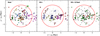 |
Fig. 1 Projected spatial distribution of galaxies in a simulated TNG100 cluster at z = 0, of r200 = 1.3 Mpc and M200 = 2.5 × 10¹⁴ M⊙. In all panels, coordinates are in Mpc from the cluster center, defined as the position of the particle with the minimum gravitational potential energy, the red circle represents the virial radius r200, and the dashed black circle highlights the position of a real group of galaxies that we discuss in the text. Left: crosses correspond to the galaxies that were accreted as part of groups, and gray dots identify the galaxies that entered the cluster individually. Center: circles of different colors identify galaxies assigned to different substructures by DS+ in its no-overlapping mode, the circle sizes being proportional to the individual probability of each DS+ group. Gray dots represent galaxies that were not assigned to any substructure. Right: green squares identify galaxies in real groups that are correctly assigned to substructures by the DS+ method, red crosses indicate galaxies that entered the cluster alone and are incorrectly assigned to substructures, and small black dots identify galaxies that were accreted as part of real groups, but were not assigned to substructures by DS+. |
4 Testing DS+ on simulated clusters
We applied the DS+ method to the 14 simulated halos observed at the present time, considering the information about the infall of their groups since ~8 Gyr ago. We considered each of the three orthogonal projections to be an individual cluster for a total of 42 galaxy clusters used in our analysis. Our aim was to identify those galaxies that entered the cluster in groups of at least three members, using only projected coordinates and l.o.s. velocities. Hereafter we use the term “real groups” to refer to the galaxies that were part of groups identified in the simulations at high redshift (before the infall) and the term “substructures” for the groups identified by DS+, using the information of l.o.s. velocities and 2D spatial coordinates (at a redshift of interest).
In Fig. 1, we show one cluster at the last time in the simulation, distinguishing between galaxies that entered the cluster as individuals and galaxies that entered the cluster in groups. A large fraction of the cluster galaxies were accreted in groups (~60%; see Benavides et al. 2020), and it is certainly impossible to identify all of them as substructures as many are well mixed with the cluster galaxies that entered the cluster individually. In the central panel of Fig. 1, we show the substructures, and in the right panel, we compare the real groups and the substructures that were identified by our method. Another example was added in Fig. B.1 in the appendix for the evolution of the same cluster. In this figure, we present similar information for each ~2 Gyr in look-back time.
4.1 Completeness and purity
A more general assessment of the performance of our method can be gained by evaluating the completeness and purity of the samples of galaxies in real groups and substructures, respectively. We call completeness, C, the fraction of galaxies in real groups that are also detected as members of any substructure
 (4)
(4)
and purity, P, the fraction of galaxies in detected substructures that belong to any real group
 (5)
(5)
In Fig. 2, we show C as a function of different variables: Richness, that is, the number of galaxies of the real groups that are detected as members of the DS+ groups, the 2D projected distance from the center of the cluster in units of the virial radius4 (R/r200), and the time since group infall into the cluster5. C ~ 0.8 for the overlapping mode of DS+. C is lower (~0.5) for the no-overlapping mode, as expected given that in this mode, we discard all substructures that have galaxies in common with more significant substructures. The fact that C values close to 1 are not observed (in particular in the non-overlapping mode) corresponds to the fact that the actual groups that fell into a cluster tend to disperse significantly after the first pericentric passage (Choque-Challapa et al. 2019; Benavides et al. 2020; Haggar et al. 2023).
The completeness C does not show a strong dependence on group richness, projected cluster-centric distance, or time since infall. For the overlapping mode, C only mildly increases with richness, reaching a value of ~0.9 for groups of ~40 members. In the no-overlapping mode, C mildly increases with group distance from the cluster center. The increasing trends of C with group richness and projected clustercentric distance are expected since richer groups offer better statistics for detection, and at larger cluster-centric distances, the density contrast of the groups is higher relative to the cluster.
The dependence of C on the time since infall is weaker than would be expected from the fact that infalling groups double their size ~1–3 Gyr after infall (depending on the group mass; Benavides et al. 2020), and in many cases are completely destroyed after their first passage through the pericenter. However, the collisionless nature of the group galaxies allows them to retain a mostly consistent velocity even after pericenter passage. This allows them to be identified as members of substructures (even if they are not in a single one), allowing C not to drop too rapidly with time since infall.
As an example, the substructure represented by the dark green crosses in the left panel of Fig. 1 (highlighted with the dashed black circle) corresponds to a substructure detected by DS+ and is indicated by light purple dots in the middle panel of the same figure. However, in other cases, real group galaxies are not associated with any substructure (small black circles in the right panel), or they are associated with many substructures and not, in the main part, to a single one (e.g., the group represented by the magenta crosses in the left panel). This occurs because the group has already crossed the center of the cluster, experiencing strong tidal forces that deform the shape of the primitive association.
In Fig. 3, we show P as a function of the same variables as in Fig. 2. There is no strong dependence of P on the mode of operation (with or without overlapping), which shows that when we ran the DS + method in the overlapping mode, we did not add substantial noise to the purity result of the detected DS+ groups. This is important for the estimate of the properties of group galaxies.
The purity P is higher than 60% and can approach 100% in some cases. It decreases as group richness increases, from 80% to just over 60%. However, this slight decreasing trend does not seem very significant, so the purity could be considered more or less flat, around ~70% for any multiplicity.
P increases significantly with the projected distance from the cluster center to the outskirts, from ~60% near the cluster center to almost 100% beyond the virial radius. It is to be expected that at large distances from the cluster center (where the cluster density is sufficiently low), the contamination of the substructure by cluster members that are not in groups would be less significant. Many of these DS+ substructures would correspond to recent accretions or to fragments of real groups that are close to their first apocenter. P also shows a clear decreasing trend with time since infall. The reason probably is that when a group crosses the cluster, its size increases considerably by tidal effects, allowing more interlopers to contaminate the region occupied by the group in projection.
The results presented above were obtained using an upper probability limit of 0.01. Similar values of C and P were obtained when considering lower probability limits (e.g., 0.005), although with fewer DS+ substructures.
It is interesting to briefly compare our results with those obtained for the recently developed Blooming Tree, which has been claimed to be the best substructure-identification method, and superior to σ plateau (Yu et al. 2018). A direct comparison is not possible because different simulations were used and the definitions of completeness and purity are different (“success rate” in Yu et al. 2018). Summarizing from the results of Yu et al. (2018), Blooming Tree reaches a completeness C ~ 0.8, and a purity, P ~ 0.6, for about half of the detected structures. The completeness of Blooming Tree is therefore comparable to that of DS+ in its overlapping mode, and superior to that of our method in its no-overlapping mode. The purity of DS+ substructures appears to be superior to that of Blooming Tree, since the value P = 0.6 is reached by the latter method only for about half of the detected structures. Pending a more direct comparison between Blooming Tree and DS+, which is beyond the scope of this paper, we tentatively conclude that these two algorithms reach similar performances in the detection of substructures.
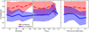 |
Fig. 2 Completeness C of member galaxies of real groups in simulated TNG100 clusters detected by DS+ groups. In all panels, the dashed red line indicates the average over all clusters, using the overlapping mode, and the solid blue line refers to the no-overlapping mode. The filled areas indicate one standard deviation. In all cases, the curves correspond to the stacking of all analyzed clusters. Left: C as a function of the richness of the real groups, corresponding to the number of galaxies detected in substructures. Center: C as a function of the real group cluster-centric distance. Right: C as a function of the time since group infall. |
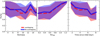 |
Fig. 3 Purity P of DS+ detected substructures in simulated TNG100 clusters. Lines and colors have the same meaning as in Fig. 2. The quantities on the x-axis of the three panels are the same as in Fig. 2. |
4.2 DS+ substructures versus real group internal properties
In order to have an additional estimate of the characteristics and reliability of the groups detected using the DS+ method, we compared several of the global properties of the detected substructures with those of their corresponding real groups, as detailed below. The global properties we considered are the l.o.s. mean velocity and velocity dispersion, the 2D size of the group (as measured by the harmonic mean radius), and the total stellar mass.
The properties of each DS+ substructure were evaluated using all galaxies assigned to that substructure. Since substructure members can be members of more than one real group, we only considered the group that had the largest number of members in common with the considered substructure. We then computed the properties of this real group using only members that were also members of the substructure. This was done because many of its original group members are rapidly dispersed into the cluster after infall, and attributing them to the group would not be correct in physical terms.
The mean values of the ratios of the substructure and group properties are given in Table 1. In all cases, the ratios are above unity, but with considerable dispersions. The DS+ estimates of both the velocity dispersion and the stellar mass of the groups are strongly overestimated, as expected because of interlopers in the substructures.
In Fig. 4, we show the correlations between the properties of the substructures and those of the corresponding real groups. In each panel, we include the mean values of the property differences Δlog(X) = log(XDS+) − log(XReal) and their standard deviation. According to the Spearman correlation coefficient, all correlations are significant with 0.94 to 0.99 probabilities (the lowest value is for the velocity dispersion). These values indicate that we can use the properties of the detected DS+ substructures to predict the properties of the corresponding real groups. However, this is only true on average, as the inferred properties may be very different from the real ones for individual groups. Galaxy properties such as stellar population or metallicity could be used to identify and remove group interlopers to improve the correspondence between group and substructure global properties. However, we did not explore this possibility in this analysis.
Mean ratios of the properties of DS+ substructures and of real groups.
5 Application to the Bullet cluster
As a practical example of our DS+ method, we applied it to the famous Bullet cluster IE 0657–558 (Barrena et al. 2002; Markevitch et al. 2002; Clowe et al. 2004). We collected spectroscopic data for galaxies in the cluster region from the NASA/IPAC Extragalactic Database (NED6). After removing double entries, we found 231 galaxies with red-shifts within a circle of 10′ radius around the cluster center. All these galaxies are members of the cluster, according to the Clean procedure of Mamon et al. (2013). The mean cluster redshift is  , and the rest-frame velocity dispersion is
  . These values were obtained using the biweight estimator as recommended by Beers et al. (1990) for large data sets. These values are consistent with those determined by Barrena et al. (2002) using 78 cluster members.
Given συ, we estimated the Bullet cluster M200 using two scaling relations of Munari et al. (2013), the relation of Eq. (1) in that paper, that is, based on the NFW profile, and the relation labeled “AGN gal” in Table 1 of that paper, that is, based on the galaxies identified in hydrodynamical simulations with AGN feedback. We obtain M200 = 1.3 ± 0.2 × 10¹⁵ M⊙ by considering the average of the values obtained using the two scaling relations. Our M200 value agrees within 1 σ with the virial mass estimate obtained by Barrena et al. (2002), and also with the mass estimate obtained from gravitational lensing (Clowe et al. 2004; Springel & Farrar 2007).
We ran the DS+ algorithm in the no-overlapping mode to the data set of 191 member galaxies within the cluster virial radius r200 = 2.1 Mpc. We found ten substructures with a formal probability p ≤ 0.01. We identified 77 galaxies as members of these substructures, and based on our DS+ purity estimate, we expect only ~50 of them to be also members of real groups. It is conceivable that many of the ~27 spurious members are those assigned to the two substructures of lowest significance, characterized by p values (0.008 and 0.010) much higher than those of the other eight substructures (≤0.003).
The properties of the ten detected substructures are listed in Table 2, and their projected spatial distribution is shown in Fig. 5. Since we work with small data sets (fewer than 15 members per substructure), we estimated the substructure velocity dispersions σg by the gapper method (Beers et al. 1990; Girardi et al. 1993). Based on our analysis of Sect. 4.2, we expect the group velocity dispersions to be 1.8 times lower on average than the corresponding substructure estimates (see Table 1).
Substructure 6 in Table 2 is the Bullet that gives the name to the cluster. Compared to the substructure identified by Barrena et al. (2002), our substructure mean velocity in the cluster rest frame is slightly lower than but still consistent with that of Barrena et al. (2002). After correcting the observed value of the substructure velocity dispersion for the average bias factor listed in Table 1, we estimate that the Bullet group should be characterized by a velocity dispersion of 472 km s−1, about twice higher than the estimate of Barrena et al. (2002).
We applied the scaling relations of Munari et al. (2013) to this corrected group velocity dispersion to estimate a group mass of  . This agrees with the weak-lensing mass estimate by Bradač et al. (2006), 2.0 ± 0.2 × 10¹⁴. The Bullet group to cluster mass ratio we find is
  , consistent with the value of 0.1 that was adopted in the numerical simulation of Springel & Farrar (2007).
In line with previous analyses (Barrena et al. 2002; Springel & Farrar 2007; Mastropietro & Burkert 2008), we here considered the classical two-body model to explore the properties of the Bullet collision (Gregory & Thompson 1984; Beers et al. 1991). Taking the mass of the cluster and the group as we inferred from kinematics, the allowed 1 σ range of the angle between the collision axis and the plane of the sky is ~4°–10° (see Fig. 6). However, the precision of this estimate is certainly too optimistic because we did not account for the systematic uncertainties inherent to the two-body model.
We then applied the MCMAC code of Dawson (2013). At variance with the classical two-body model, the method developed by Dawson (2013) does not assume that the colliding systems are point masses. The cluster and the group are modeled as two spherically symmetric NFW halos. The model assumes energy conservation, zero impact parameter, and that the maximum relative velocities of the two systems is the free-fall velocity given their estimated masses. Dynamical friction is not included in the model. The model is incorporated in a Monte Carlo implementation, wherein parameter values are drawn randomly from observables with associated uncertainties. The observables are the masses of the colliding systems, their mass concentrations, mean redshifts, and the projected distance between the two.
As before, we adopted the masses and uncertainties we derived from the cluster and group velocity dispersions. We did not measure their mass concentrations, and we therefore adopted the mass-concentration relation of Duffy et al. (2008), which is the internal default of the MCMAC code. We ran 50 000 Monte Carlo resamplings. In Fig. 7 we show the results as 68% confidence regions in the plane of “time since the collision” versus “relative 3D velocity at the collision time”. The green contour corresponds to the solution obtained with no external constraint on the angle of the collision. When we discard the solutions with a collision angle outside the range ~4°–10° suggested by the two-body model (Fig. 6), we obtain the orange contour in Fig. 7. As explained above, the allowed range for the collision angle that we infer from the two-body model is too restrictive because it ignores systematic uncertainties. Another possibly more reliable estimate of the allowed collision angle has been derived by Wittman et al. (2018) based on the identification of analogs of observed systems in cosmological N-body simulations. They constrained the collision angle of the Bullet to be ≤29° at the 68% confidence level. Inserting this constraint in our MCMAC solution gives the red contour in Fig. 7.
From the MCMAC analysis, we conclude that the observational uncertainties are currently too large to allow strong constraints on the geometry, timing, and kinematics of the Bullet collision. Our results suggest that the collision occurred within the last 500 Myr, and that the highest Bullet collision speed was in the range ~2000–1000 km s−1. The Bullet velocity we find is therefore significantly lower than the velocity of the bow shock preceding the Bullet (4700 km s−1; Markevitch 2006), as expected from numerical simulations (Milosavljevic et al. 2007; Springel & Farrar 2007). According to Thompson et al. (2015), a collision of two massive systems such as the Bullet cluster and group, with a collision velocity of ~3000 km s−1, is a rare but not impossible event in a ΛCDM cosmology.
Our DS+ analysis identifies another (previously unidentified) seven substructures with a DS+ probability similar to that of the Bullet (see Table 2; we ignore the two substructures of lowest significance in the following discussion). Some have very high velocity dispersion estimates, but are not incompatible with typical group values, given the large error bars and that they are expected to be overestimated by a bias factor of 1.8 on average (see Table 1).
Substructure 3 lies along the Bullet collision axis (as inferred from X-ray images; Markevitch et al. 2002). Its velocity is much higher but compatible within the uncertainties than that of the Bullet (see Table 2 and the right panel of Fig. 5), so that it might be originating from the same (as yet unidentified) large-scale structure filament whence the Bullet itself came from. The main cluster axis, almost orthogonal to the Bullet collision axis, is traced by four substructures (substructures 2, 7, 4, and 1, from bottom left to top right in Fig. 5). The elongation of the cluster has been suggested to indicate another merger axis for the cluster (Lage & Farrar 2014; Sikhosana et al. 2023). Our detection of substructures along this axis lends support to this hypothesis, although the lack of a coherent velocity pattern along this (hypothetical) merger axis (see Fig. 5, right panel) suggests that multiple episodes of accretion have occurred already along the same axis, with some groups observed before and some after their pericenter passages. Substructure 5 does not seem to be related to either of the two main collision axes.
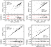 |
Fig. 4 Comparison of different properties of the DS+ no-overlapping substructures with the corresponding ones of the real groups matched to the detected substructures. Top left: mean l.o.s. velocities. Top right: l.o.s. velocity dispersions. Bottom left: projected group size (mean harmonic radius). Bottom right: total stellar mass. In each panel, we include the mean and standard deviation of the differences between the substructure and the matched real group properties. The lower sub-panels show the logarithm of the ratio of the substructure and group properties, and the dotted red lines indicate 50% variations with respect to the ratio of unity. |
Properties of detected Bullet cluster substructures.
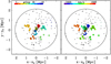 |
Fig. 5 Projected spatial distribution of Bullet member galaxies. North is up, east is to the left. The large black circle has a radius of r200 = 2.13 Mpc and is centered on the cluster center, RA = 104.65139, Dec = −55.95468. Smaller circles (crosses) represent galaxies assigned (not assigned) to substructures by DS+. The size of the circles scales as 1–100 p, where p is the probability of the detected group listed in Table 2. Left panel: different colors identify galaxies assigned to different groups, numbered 1 to 10 as in the inset bar and Table 2. Group 6 is the Bullet, represented by the nine turquoise dots at coordinates (−0.74, 0.22). Right panel: color scale represents the mean velocity of the groups (see Table 2). |
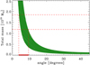 |
Fig. 6 Two-body collision model between the main cluster and the Bullet (group 6 in Table 2). The total mass of the system is shown on the y-axis as a function of the angle of the collision axis with respect to the plane of the sky. The estimated total mass range (1 σ) is illustrated by the two dashed lines. At the intersection of these lines with the model curve, we draw two vertical lines that identify the inferred allowed collision angles (in green on the x-axis), ~4°–10°. |
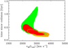 |
Fig. 7 Result of the MCMAC algorithm (Dawson 2013) applied to the Bullet cluster and its bullet (group 6 in Table 2), time since collision vs. 3D velocity at the time of the collision. Contours are 68% confidence levels. Green contours do not include any constraint on the collision angle. Red contours are obtained by considering only angles ≤29°, i.e., the 1 σ constraint derived by Wittman et al. (2018). Orange contours are obtained by considering only angles between 3° and 10°, as inferred from the classical two-body collision model. |
6 Summary and conclusions
We presented a new method for the identification and characterization of group-sized substructures in clusters of galaxies. Our new method, DS+, is based on the positions and velocities of cluster galaxies, and it is an improvement and extension of the traditional method of Dressler & Shectman (1988). The method does not provide a global measure of the number of substructures in a cluster, as most methods do, but identifies the galaxies that belong to substructures and the substructure themselves. The method can be run in two modes: overlapping, and no-overlapping. The first mode allows the most complete identification of galaxies in substructures, and the second operational mode allows us to uniquely identify substructures as independent galaxy associations.
We tested DS+ on cosmological halos of cluster size extracted from the IllustrisTNG simulation, where infalling groups have been identified by the FoF technique. On average, each of these halos contains 190 galaxies down to a stellar mass of 1.5 × 10⁸ M⊙. We find that our method (run in its overlapping mode) successfully identified ~80% of the group galaxies as members of substructures, even in groups with fewer than ten member galaxies. At least 60% of the galaxies assigned to the detected substructures are also members of real groups.
We then compared the properties of the detected substructures in the no-overlapping mode of DS+ with those of the matched real groups by associating the group with the largest number of common galaxies with each detected substructure. We find that the mean velocity, size, velocity dispersion, and stellar mass of the detected substructures are significantly correlated with the corresponding properties of the matched groups, but with a large scatter and a substantial bias. It is then possible to use the properties of the detected substructures to learn about the properties of the real groups, but only on average, by taking into account the biases.
We applied the DS+ method to the Bullet cluster as an example. We find ten significant substructures, one of which corresponds to the group for which the cluster is named. We studied the geometry and kinematics of the Bullet collision and find consistent results with previous studies, setting 68% confidence limits to the collision velocity (2000–4000 km s−1 ) and the collision time (≲0.5 Gyr). The other detected substructures suggest the presence of another collision axis that corresponds to the main southeast to northwest elongation of the cluster.
We conclude that DS+ is a reliable and useful method for the identification of substructure galaxies and substructures themselves in clusters. A Python implementation of our method is freely available for use in GitHub.
Acknowledgements
A.B. thanks Peter Katgert, for his precious collaboration in past years on the development of a method for the detection of cluster substructures. This work was largely supported by the LACEGAL program. J.B. and M.A. acknowledge financial support from FONCYT, Argentina through PICT 20191600. This research has made use of the NASA/IPAC Extragalactic Database (NED), which is funded by the National Aeronautics and Space Administration and operated by the California Institute of Technology.
Appendix A Brief description of how the DS+ public code can be used
Here we present a brief description of the DS+ code in the python public version, which are available in the GitHub repository7. The DS+ method has been implemented as the main function into the MilaDS code. Briefly, the principal inputs of the code are the spatial x,y coordinates in kiloparsec, the l.o.s. velocities, the redshift of the cluster, and, as an option, the number of resamplings Nsims (nsims) that use random samples to assess the probability of the detected substructures, and the upper limit probability (Plim_P) below which the detections are considered significant.
DSp_groups is the main function of MilaDS that receives input information and processes three principal (sequential) stages:
Individual probability of each galaxy to belong to some DS+ group of any multiplicity.
Allocation of each galaxy to only one DS+ group, following the Plim priority. Assign each DS+ group one unique group number, so that galaxies outside of the final group allocation possess group number GrNr = −1, and zero in their group properties.
Summary of DS+ groups properties, such as group number (GrNr), number of galaxies in each group (Ngal), radial cluster-centric distance (R in kpc), group size (size in kpc), velocity dispersions of the group (sigma km/s), mean velocity of the group (Vmean in km/s), minimum probability of the group (Pmin), and an average of individual probabilities of all galaxies in each DS+ detected group (Pmin_avr).
The shortest running form of the DS+ code for a cluster located at z=0.296 using 500 re-simulations and an upper probability limit of 1% is as follows:
# import MilaDS and other packages
>>> import milaDS
>>> import numpy as np
>>> my_data = np.genfromtxt (“cluster_C1.dat”)
… # 0:galaxies IDs
… # 1:X in kpc
… # 2:Y in kpc
… # 3:rest-frame Vel (V_los) in km/s
>>> data_DSp, data_grs_alloc, summary_DSp_grs =
…         milaDS.DSp_groups(
…               Xcoor=my_data[:,1],
…               Ycoor=my_data[:,2],
…               Vlos=my_data[:,3],
…               Zclus=0.296,
…               cluster_name=“C1”,
…               nsims=500,
…               Plim_P=1 )
Appendix B DS+ in the accretion history
Here we present the projected spatial distribution of the galaxies in the same simulated cluster as shown in Fig. 1 at different time snapshots since z = 0 (top panel) and separated by ~2 Gyr. The colors are reset at each snapshot, so that it would not be entirely correct to track groups along different time snapshots based on their colors.
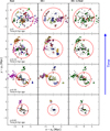 |
Fig. B.1 Same cluster as presented in Fig. 1, but for different time snapshots, starting at z = 0 (top panel) and each ~2 Gyr look-back in time, until z ~ 0.62 (bottom panel). Coordinates are in Mpc from the cluster center, defined as the position of the particle with the minimum gravitational potential energy, and the red circle indicates the virial radius of the cluster at the corresponding time. |
References
- Abdelsalam, H. M., Saha, P., & Williams, L. L. R. 1998, AJ, 116, 1541 [NASA ADS] [CrossRef] [Google Scholar]
- Akamatsu, H., Gu, L., Shimwell, T. W., et al. 2016, A&A, 593, A7 [Google Scholar]
- Andersson, K., Peterson, J. R., Madejski, G., & Goobar, A. 2009, ApJ, 696, 1029 [NASA ADS] [CrossRef] [Google Scholar]
- Andrade-Santos, F., Lima Neto, G. B., & Laganá, T. F. 2012, ApJ, 746, 139 [NASA ADS] [CrossRef] [Google Scholar]
- Angrick, C., & Bartelmann, M. 2012, A&A, 538, A98 [NASA ADS] [CrossRef] [EDP Sciences] [Google Scholar]
- Asencio, E., Banik, I., & Kroupa, P. 2021, MNRAS, 500, 5249 [Google Scholar]
- Barrena, R., Biviano, A., Ramella, M., Falco, E. E., & Seitz, S. 2002, A&A, 386, 816 [NASA ADS] [CrossRef] [EDP Sciences] [Google Scholar]
- Barrena, R., Girardi, M., & Boschin, W. 2013, MNRAS, 430, 3453 [NASA ADS] [CrossRef] [Google Scholar]
- Bartalucci, I., Arnaud, M., Pratt, G. W., Démoclès, J., & Lovisari, L. 2019, A&A, 628, A86 [EDP Sciences] [Google Scholar]
- Beers, T. C., Flynn, K., & Gebhardt, K. 1990, AJ, 100, 32 [Google Scholar]
- Beers, T. C., Gebhardt, K., Forman, W., Huchra, J. P., & Jones, C. 1991, AJ, 102, 1581 [NASA ADS] [CrossRef] [Google Scholar]
- Bekki, K. 1999, ApJ, 510, L15 [NASA ADS] [CrossRef] [Google Scholar]
- Bellhouse, C., Poggianti, B., Moretti, A., et al. 2022, ApJ, 937, 18 [NASA ADS] [CrossRef] [Google Scholar]
- Benavides, J. A., Sales, L. V., & Abadi, M. G. 2020, MNRAS, 498, 3852 [Google Scholar]
- Bird, C. M. 1994, AJ, 107, 1637 [Google Scholar]
- Biviano, A., Katgert, P., Thomas, T., & Adami, C. 2002, A&A, 387, 8 [NASA ADS] [CrossRef] [EDP Sciences] [Google Scholar]
- Biviano, A., Murante, G., Borgani, S., et al. 2006, A&A, 456, 23 [NASA ADS] [CrossRef] [EDP Sciences] [Google Scholar]
- Biviano, A., Moretti, A., Paccagnella, A., et al. 2017, A&A, 607, A81 [NASA ADS] [CrossRef] [EDP Sciences] [Google Scholar]
- Boschin, W., & Girardi, M. 2018, MNRAS, 480, 1187 [NASA ADS] [CrossRef] [Google Scholar]
- Bradac, M., Clowe, D., Gonzalez, A. H., et al. 2006, ApJ, 652, 937 [CrossRef] [Google Scholar]
- Briel, U. G., Henry, J. P., & Boehringer, H. 1992, A&A, 259, L31 [NASA ADS] [Google Scholar]
- Buote, D. A., & Tsai, J. C. 1995, ApJ, 452, 522 [Google Scholar]
- Burgett, W. S., Vick, M. M., Davis, D. S., et al. 2004, MNRAS, 352, 605 [NASA ADS] [CrossRef] [Google Scholar]
- Campitiello, M. G., Ettori, S., Lovisari, L., et al. 2022, A&A, 665, A117 [NASA ADS] [CrossRef] [EDP Sciences] [Google Scholar]
- Cao, K., Barnes, D. J., & Vogelsberger, M. 2021, MNRAS, 503, 3394 [NASA ADS] [CrossRef] [Google Scholar]
- Chon, G., Böhringer, H., & Smith, G. P. 2012, A&A, 548, A59 [NASA ADS] [CrossRef] [EDP Sciences] [Google Scholar]
- Choque-Challapa, N., Smith, R., Candlish, G., Peletier, R., & Shin, J. 2019, MNRAS, 490, 3654 [NASA ADS] [CrossRef] [Google Scholar]
- Clowe, D., Gonzalez, A., & Markevitch, M. 2004, ApJ, 604, 596 [NASA ADS] [CrossRef] [Google Scholar]
- Clowe, D., Schneider, P., Aragón-Salamanca, A., et al. 2006, A&A, 451, 395 [NASA ADS] [CrossRef] [EDP Sciences] [Google Scholar]
- Colless, M., & Dunn, A. M. 1996, ApJ, 458, 435 [Google Scholar]
- Davis, M., Efstathiou, G., Frenk, C. S., & White, S. D. M. 1985, ApJ, 292, 371 [Google Scholar]
- Dawson, W. A. 2013, ApJ, 772, 131 [NASA ADS] [CrossRef] [Google Scholar]
- De Luca, F., De Petris, M., Yepes, G., et al. 2021, MNRAS, 504, 5383 [NASA ADS] [CrossRef] [Google Scholar]
- Dressler, A., & Shectman, S. A. 1988, AJ, 95, 985 [Google Scholar]
- Dubinski, J. 1999, ASP Conf. Ser., 182, 491 [NASA ADS] [Google Scholar]
- Duffy, A. R., Schaye, J., Kay, S. T., & Dalla Vecchia, C. 2008, MNRAS, 390, L64 [Google Scholar]
- Einasto, M., Tago, E., Saar, E., et al. 2010, A&A, 522, A92 [NASA ADS] [CrossRef] [EDP Sciences] [Google Scholar]
- Einasto, M., Vennik, J., Nurmi, P., et al. 2012, A&A, 540, A123 [NASA ADS] [CrossRef] [EDP Sciences] [Google Scholar]
- Einasto, M., Gramann, M., Park, C., et al. 2018, A&A, 620, A149 [NASA ADS] [CrossRef] [EDP Sciences] [Google Scholar]
- Einasto, M., Kipper, R., Tenjes, P., et al. 2021, A&A, 649, A51 [NASA ADS] [CrossRef] [EDP Sciences] [Google Scholar]
- Escalera, E., Biviano, A., Girardi, M., et al. 1994, ApJ, 423, 539 [NASA ADS] [CrossRef] [Google Scholar]
- Ferrari, C., Maurogordato, S., Cappi, A., & Benoist, C. 2003, A&A, 399, 813 [NASA ADS] [CrossRef] [EDP Sciences] [Google Scholar]
- Ferrari, C., Benoist, C., Maurogordato, S., Cappi, A., & Slezak, E. 2005, A&A, 430, 19 [NASA ADS] [CrossRef] [EDP Sciences] [Google Scholar]
- Fischer, M. S., Brüggen, M., Schmidt-Hoberg, K., et al. 2022, MNRAS, 510, 4080 [NASA ADS] [CrossRef] [Google Scholar]
- Forero-Romero, J. E., Gottlöber, S., & Yepes, G. 2010, ApJ, 725, 598 [NASA ADS] [CrossRef] [Google Scholar]
- Fraley, C., & Raftery, A. E. 2006, Technical Report, Dept. of Statistics, University of Washington, 504, 1 [Google Scholar]
- Gal, R. R., Lopes, P. A. A., de Carvalho, R. R., et al. 2009, AJ, 137, 2981 [NASA ADS] [CrossRef] [Google Scholar]
- Gebhardt, K., Pryor, C., Williams, T. B., & Hesser, J. E. 1994, AJ, 107, 2067 [NASA ADS] [CrossRef] [Google Scholar]
- Geller, M. J., & Beers, T. C. 1982, PASP, 94, 421 [NASA ADS] [CrossRef] [Google Scholar]
- Ghirardini, V., Bahar, Y. E., Bulbul, E., et al. 2022, A&A, 661, A12 [NASA ADS] [CrossRef] [EDP Sciences] [Google Scholar]
- Girardi, M., & Biviano, A. 2002, in Optical Analysis of Cluster Mergers, Merging Processes in Galaxy Clusters, ed. L. Feretti, I. M. Gioia, & G. Giovannini (The Netherlands: Kluwer Ac. Pub.), 39 [CrossRef] [Google Scholar]
- Girardi, M., Biviano, A., Giuricin, G., Mardirossian, F., & Mezzetti, M. 1993, ApJ, 404, 38 [NASA ADS] [CrossRef] [Google Scholar]
- Girardi, M., Demarco, R., Rosati, P., & Borgani, S. 2005, A&A, 442, 29 [NASA ADS] [CrossRef] [EDP Sciences] [Google Scholar]
- Girardi, M., Bardelli, S., Barrena, R., et al. 2011, A&A, 536, A89 [NASA ADS] [CrossRef] [EDP Sciences] [Google Scholar]
- Girardi, M., Mercurio, A., Balestra, I., et al. 2015, A&A, 579, A4 [NASA ADS] [CrossRef] [EDP Sciences] [Google Scholar]
- Gnedin, O. Y. 1999, Ph.D. Thesis, Princeton University, New Jersey, USA [Google Scholar]
- Golovich, N., Dawson, W. A., Wittman, D. M., et al. 2019, ApJ, 882, 69 [NASA ADS] [CrossRef] [Google Scholar]
- Gregory, S. A., & Thompson, L. A. 1984, ApJ, 286, 422 [NASA ADS] [CrossRef] [Google Scholar]
- Gurzadyan, V. G., Harutyunyan, V. V., & Kocharyan, A. A. 1994, A&A, 281, 964 [NASA ADS] [Google Scholar]
- Haggar, R., Kuchner, U., Gray, M. E., et al. 2023, MNRAS, 518, 1316 [Google Scholar]
- Hashimoto, Y., Böhringer, H., Henry, J. P., Hasinger, G., & Szokoly, G. 2007, A&A, 467, 485 [NASA ADS] [CrossRef] [EDP Sciences] [Google Scholar]
- Hwang, H. S., & Lee, M. G. 2007, ApJ, 662, 236 [NASA ADS] [CrossRef] [Google Scholar]
- Jauzac, M., Eckert, D., Schwinn, J., et al. 2016, MNRAS, 463, 3876 [NASA ADS] [CrossRef] [Google Scholar]
- King, L. J., Clowe, D. I., Coleman, J. E., et al. 2016, MNRAS, 459, 517 [NASA ADS] [CrossRef] [Google Scholar]
- Kolokotronis, V., Basilakos, S., Plionis, M., & Georgantopoulos, I. 2001, MNRAS, 320, 49 [NASA ADS] [CrossRef] [Google Scholar]
- Laganá, T. F., Souza, G. S., Machado, R. E. G., Volert, R. C., & Lopes, P. A. A. 2019, MNRAS, 487, 3922 [CrossRef] [Google Scholar]
- Lage, C., & Farrar, G. 2014, ApJ, 787, 144 [NASA ADS] [CrossRef] [Google Scholar]
- Leonard, A., Goldberg, D. M., Haaga, J. L., & Massey, R. 2007, ApJ, 666, 51 [NASA ADS] [CrossRef] [Google Scholar]
- Lopes, P. A. A., de Carvalho, R. R., Capelato, H. V., et al. 2006, ApJ, 648, 209 [NASA ADS] [CrossRef] [Google Scholar]
- Lopes, P. A. A., Trevisan, M., Laganá, T. F., et al. 2018, MNRAS, 478, 5473 [Google Scholar]
- Macciò, A. V., Dutton, A. A., & van den Bosch, F. C. 2008, MNRAS, 391, 1940 [Google Scholar]
- Mahajan, S. 2013, MNRAS, 431, L117 [NASA ADS] [CrossRef] [Google Scholar]
- Mamon, G. A., Biviano, A., & Murante, G. 2010, A&A, 520, A30 [NASA ADS] [CrossRef] [EDP Sciences] [Google Scholar]
- Mamon, G. A., Biviano, A., & Boué, G. 2013, MNRAS, 429, 3079 [Google Scholar]
- Markevitch, M. 2006, in Proceedings of The X-ray Universe 2005, ed. A. Wilson (ESA), 723 [Google Scholar]
- Markevitch, M., Gonzalez, A. H., David, L., et al. 2002, ApJ, 567, L27 [Google Scholar]
- Markevitch, M., Gonzalez, A. H., Clowe, D., et al. 2004, ApJ, 606, 819 [NASA ADS] [CrossRef] [Google Scholar]
- Martinet, N., Clowe, D., Durret, F., et al. 2016, A&A, 590, A69 [NASA ADS] [CrossRef] [EDP Sciences] [Google Scholar]
- Mastropietro, C., & Burkert, A. 2008, MNRAS, 389, 967 [NASA ADS] [CrossRef] [Google Scholar]
- Mauduit, J.-C., & Mamon, G. A. 2007, A&A, 475, 169 [NASA ADS] [CrossRef] [EDP Sciences] [Google Scholar]
- Maughan, B. J., Jones, C., Forman, W., & Van Speybroeck, L. 2008, ApJS, 174, 117 [NASA ADS] [CrossRef] [Google Scholar]
- Merten, J., Coe, D., Dupke, R., et al. 2011, MNRAS, 417, 333 [NASA ADS] [CrossRef] [Google Scholar]
- Miller, N. A., Owen, F. N., Hill, J. M., et al. 2004, ApJ, 613, 841 [NASA ADS] [CrossRef] [Google Scholar]
- Miller, C. J., Nichol, R. C., Reichart, D., et al. 2005, AJ, 130, 968 [Google Scholar]
- Milosavljevic, M., Koda, J., Nagai, D., Nakar, E., & Shapiro, P. R. 2007, ApJ, 661, L131 [NASA ADS] [CrossRef] [Google Scholar]
- Mohammed, I., Saha, P., Williams, L. L. R., Liesenborgs, J., & Sebesta, K. 2016, MNRAS, 459, 1698 [NASA ADS] [CrossRef] [Google Scholar]
- Mohr, J. J., Evrard, A. E., Fabricant, D. G., & Geller, M. J. 1995, ApJ, 447, 8 [NASA ADS] [CrossRef] [Google Scholar]
- Motl, P. M., Hallman, E. J., Burns, J. O., & Norman, M. L. 2005, ApJ, 623, L63 [Google Scholar]
- Muriel, H., Quintana, H., Infante, L., Lambas, D. G., & Way, M. J. 2002, AJ, 124, 1934 [NASA ADS] [CrossRef] [Google Scholar]
- Munari, E., Biviano, A., Borgani, S., Murante, G., & Fabjan, D. 2013, MNRAS, 430, 2638 [Google Scholar]
- Navarro, J. F., Frenk, C. S., & White, S. D. M. 1997, ApJ, 490, 493 [Google Scholar]
- Nelson, D., Pillepich, A., Springel, V., et al. 2018, MNRAS, 475, 624 [Google Scholar]
- Nelson, D., Springel, V., Pillepich, A., et al. 2019, Computat. Astrophys. Cosmol., 6, 2 [NASA ADS] [CrossRef] [Google Scholar]
- Neumann, D. M., Lumb, D. H., Pratt, G. W., & Briel, U. G. 2003, A&A, 400, 811 [NASA ADS] [CrossRef] [EDP Sciences] [Google Scholar]
- Oklopcic, A., Smolcic, V., Giodini, S., et al. 2010, ApJ, 713, 484 [NASA ADS] [CrossRef] [Google Scholar]
- Olave-Rojas, D., Cerulo, P., Demarco, R., et al. 2018, MNRAS, 479, 2328 [Google Scholar]
- Parekh, V., van der Heyden, K., Ferrari, C., Angus, G., & Holwerda, B. 2015, A&A, 575, A127 [NASA ADS] [CrossRef] [EDP Sciences] [Google Scholar]
- Pillepich, A., Nelson, D., Hernquist, L., et al. 2018a, MNRAS, 475, 648 [Google Scholar]
- Pillepich, A., Springel, V., Nelson, D., et al. 2018b, MNRAS, 473, 4077 [Google Scholar]
- Pinkney, J., Roettiger, K., Burns, J. O., & Bird, C. M. 1996, ApJS, 104, 1 [NASA ADS] [CrossRef] [Google Scholar]
- Pisani, A. 1993, MNRAS, 265, 706 [NASA ADS] [Google Scholar]
- Pisani, A. 1996, MNRAS, 278, 697 [NASA ADS] [CrossRef] [Google Scholar]
- Planck Collaboration XIII. 2016, A&A, 594, A13 [NASA ADS] [CrossRef] [EDP Sciences] [Google Scholar]
- Poggianti, B. M., Bridges, T. J., Komiyama, Y., et al. 2004, ApJ, 601, 197 [NASA ADS] [CrossRef] [Google Scholar]
- Prokhorov, D. A., & Durret, F. 2007, A&A, 474, 375 [NASA ADS] [CrossRef] [EDP Sciences] [Google Scholar]
- Ramella, M., Biviano, A., Pisani, A., et al. 2007, A&A, 470, 39 [NASA ADS] [CrossRef] [EDP Sciences] [Google Scholar]
- Ribeiro, A. L. B., de Carvalho, R. R., Trevisan, M., et al. 2013a, MNRAS, 434, 784 [NASA ADS] [CrossRef] [Google Scholar]
- Ribeiro, A. L. B., Lopes, P. A. A., & Rembold, S. B. 2013b, A&A, 556, A74 [NASA ADS] [CrossRef] [EDP Sciences] [Google Scholar]
- Richstone, D., Loeb, A., & Turner, E. L. 1992, ApJ, 393, 477 [NASA ADS] [CrossRef] [Google Scholar]
- Roberts, I. D., & Parker, L. C. 2019, MNRAS, 490, 773 [NASA ADS] [CrossRef] [Google Scholar]
- Rodriguez-Gomez, V., Genel, S., Vogelsberger, M., et al. 2015, MNRAS, 449, 49 [Google Scholar]
- Ruppin, F., McDonald, M., Brodwin, M., et al. 2020, ApJ, 893, 74 [NASA ADS] [CrossRef] [Google Scholar]
- Sampaio, V. M., de Carvalho, R. R., Ferreras, I., et al. 2021, MNRAS, 503, 3065 [NASA ADS] [CrossRef] [Google Scholar]
- Schimd, C., & Sereno, M. 2021, MNRAS, 502, 3911 [NASA ADS] [CrossRef] [Google Scholar]
- Serna, A., & Gerbal, D. 1996, A&A, 309, 65 [NASA ADS] [Google Scholar]
- Sikhosana, S. P., Knowles, K., Hilton, M., Moodley, K., & Murgia, M. 2023, MNRAS, 518, 4595 [Google Scholar]
- Soares, N. R., & Rembold, S. B. 2019, MNRAS, 483, 4354 [NASA ADS] [CrossRef] [Google Scholar]
- Springel, V. 2010, MNRAS, 401, 791 [Google Scholar]
- Springel, V. 2015, Astrophysics Source Code Library [record ascl:1502.003] [Google Scholar]
- Springel, V., & Farrar, G. R. 2007, MNRAS, 380, 911 [NASA ADS] [CrossRef] [Google Scholar]
- Springel, V., Pakmor, R., Pillepich, A., et al. 2018, MNRAS, 475, 676 [Google Scholar]
- Sunyaev, R. A., & Zeldovich, Y. B. 1969, Nature, 223, 721 [NASA ADS] [CrossRef] [Google Scholar]
- Suwa, T., Habe, A., Yoshikawa, K., & Okamoto, T. 2003, ApJ, 588, 7 [NASA ADS] [CrossRef] [Google Scholar]
- Takizawa, M., Nagino, R., & Matsushita, K. 2010, PASJ, 62, 951 [NASA ADS] [CrossRef] [Google Scholar]
- Thomas, P. A., Colberg, J. M., Couchman, H. M. P., et al. 1998, MNRAS, 296, 1061 [NASA ADS] [CrossRef] [Google Scholar]
- Thompson, R., Davé, R., & Nagamine, K. 2015, MNRAS, 452, 3030 [NASA ADS] [CrossRef] [Google Scholar]
- Tonnesen, S., & Bryan, G. L. 2008, ApJ, 684, L9 [NASA ADS] [CrossRef] [Google Scholar]
- Ventimiglia, D. A., Voit, G. M., Donahue, M., & Ameglio, S. 2008, ApJ, 685, 118 [Google Scholar]
- Vogelsberger, M., Genel, S., Springel, V., et al. 2014a, Nature, 509, 177 [Google Scholar]
- Vogelsberger, M., Genel, S., Springel, V., et al. 2014b, MNRAS, 444, 1518 [Google Scholar]
- Wen, Z. L., & Han, J. L. 2013, MNRAS, 436, 275 [Google Scholar]
- Wilber, A., Brüggen, M., Bonafede, A., et al. 2019, A&A, 622, A25 [NASA ADS] [CrossRef] [EDP Sciences] [Google Scholar]
- Wing, J. D., & Blanton, E. L. 2013, ApJ, 767, 102 [NASA ADS] [CrossRef] [Google Scholar]
- Wittman, D., Cornell, B. H., & Nguyen, J. 2018, ApJ, 862, 160 [NASA ADS] [CrossRef] [Google Scholar]
- Yu, H., Serra, A. L., Diaferio, A., & Baldi, M. 2015, ApJ, 810, 37 [NASA ADS] [CrossRef] [Google Scholar]
- Yu, H., Diaferio, A., Serra, A. L., & Baldi, M. 2018, ApJ, 860, 118 [NASA ADS] [CrossRef] [Google Scholar]
- Yuan, Z. S., Han, J. L., & Wen, Z. L. 2022, MNRAS, 513, 3013 [NASA ADS] [CrossRef] [Google Scholar]
- Zenteno, A., Hernández-Lang, D., Klein, M., et al. 2020, MNRAS, 495, 705 [Google Scholar]
- Zhang, Y.-Y., Reiprich, T. H., Finoguenov, A., Hudson, D. S., & Sarazin, C. L. 2009, ApJ, 699, 1178 [NASA ADS] [CrossRef] [Google Scholar]
- Zhang, B., Cui, W., Wang, Y., Dave, R., & De Petris, M. 2022, MNRAS, 516, 26 [NASA ADS] [CrossRef] [Google Scholar]
Extending the maximum to Nm/2 would create an ambiguity about which is the cluster and which the substructure.
The virial radius of the cluster r200 is the radius of a sphere with an overdensity 200 times the critical density of the Universe.
We followed the infall time definition of Benavides et al. (2020), that is, the last time the infalling group and the cluster were identified as different FoF systems.
The NASA/IPAC Extragalactic Database (NED) is funded by the National Aeronautics and Space Administration and operated by the California Institute of Technology.
All Tables
All Figures
|
Fig. 1 Projected spatial distribution of galaxies in a simulated TNG100 cluster at z = 0, of r200 = 1.3 Mpc and M200 = 2.5 × 10¹⁴ M⊙. In all panels, coordinates are in Mpc from the cluster center, defined as the position of the particle with the minimum gravitational potential energy, the red circle represents the virial radius r200, and the dashed black circle highlights the position of a real group of galaxies that we discuss in the text. Left: crosses correspond to the galaxies that were accreted as part of groups, and gray dots identify the galaxies that entered the cluster individually. Center: circles of different colors identify galaxies assigned to different substructures by DS+ in its no-overlapping mode, the circle sizes being proportional to the individual probability of each DS+ group. Gray dots represent galaxies that were not assigned to any substructure. Right: green squares identify galaxies in real groups that are correctly assigned to substructures by the DS+ method, red crosses indicate galaxies that entered the cluster alone and are incorrectly assigned to substructures, and small black dots identify galaxies that were accreted as part of real groups, but were not assigned to substructures by DS+. |
| In the text | |
|
Fig. 2 Completeness C of member galaxies of real groups in simulated TNG100 clusters detected by DS+ groups. In all panels, the dashed red line indicates the average over all clusters, using the overlapping mode, and the solid blue line refers to the no-overlapping mode. The filled areas indicate one standard deviation. In all cases, the curves correspond to the stacking of all analyzed clusters. Left: C as a function of the richness of the real groups, corresponding to the number of galaxies detected in substructures. Center: C as a function of the real group cluster-centric distance. Right: C as a function of the time since group infall. |
| In the text | |
|
Fig. 3 Purity P of DS+ detected substructures in simulated TNG100 clusters. Lines and colors have the same meaning as in Fig. 2. The quantities on the x-axis of the three panels are the same as in Fig. 2. |
| In the text | |
|
Fig. 4 Comparison of different properties of the DS+ no-overlapping substructures with the corresponding ones of the real groups matched to the detected substructures. Top left: mean l.o.s. velocities. Top right: l.o.s. velocity dispersions. Bottom left: projected group size (mean harmonic radius). Bottom right: total stellar mass. In each panel, we include the mean and standard deviation of the differences between the substructure and the matched real group properties. The lower sub-panels show the logarithm of the ratio of the substructure and group properties, and the dotted red lines indicate 50% variations with respect to the ratio of unity. |
| In the text | |
|
Fig. 5 Projected spatial distribution of Bullet member galaxies. North is up, east is to the left. The large black circle has a radius of r200 = 2.13 Mpc and is centered on the cluster center, RA = 104.65139, Dec = −55.95468. Smaller circles (crosses) represent galaxies assigned (not assigned) to substructures by DS+. The size of the circles scales as 1–100 p, where p is the probability of the detected group listed in Table 2. Left panel: different colors identify galaxies assigned to different groups, numbered 1 to 10 as in the inset bar and Table 2. Group 6 is the Bullet, represented by the nine turquoise dots at coordinates (−0.74, 0.22). Right panel: color scale represents the mean velocity of the groups (see Table 2). |
| In the text | |
|
Fig. 6 Two-body collision model between the main cluster and the Bullet (group 6 in Table 2). The total mass of the system is shown on the y-axis as a function of the angle of the collision axis with respect to the plane of the sky. The estimated total mass range (1 σ) is illustrated by the two dashed lines. At the intersection of these lines with the model curve, we draw two vertical lines that identify the inferred allowed collision angles (in green on the x-axis), ~4°–10°. |
| In the text | |
|
Fig. 7 Result of the MCMAC algorithm (Dawson 2013) applied to the Bullet cluster and its bullet (group 6 in Table 2), time since collision vs. 3D velocity at the time of the collision. Contours are 68% confidence levels. Green contours do not include any constraint on the collision angle. Red contours are obtained by considering only angles ≤29°, i.e., the 1 σ constraint derived by Wittman et al. (2018). Orange contours are obtained by considering only angles between 3° and 10°, as inferred from the classical two-body collision model. |
| In the text | |
|
Fig. B.1 Same cluster as presented in Fig. 1, but for different time snapshots, starting at z = 0 (top panel) and each ~2 Gyr look-back in time, until z ~ 0.62 (bottom panel). Coordinates are in Mpc from the cluster center, defined as the position of the particle with the minimum gravitational potential energy, and the red circle indicates the virial radius of the cluster at the corresponding time. |
| In the text | |
Current usage metrics show cumulative count of Article Views (full-text article views including HTML views, PDF and ePub downloads, according to the available data) and Abstracts Views on Vision4Press platform.
Data correspond to usage on the plateform after 2015. The current usage metrics is available 48-96 hours after online publication and is updated daily on week days.
Initial download of the metrics may take a while.