| Issue |
A&A
Volume 697, May 2025
|
|
|---|---|---|
| Article Number | A54 | |
| Number of page(s) | 36 | |
| Section | Stellar atmospheres | |
| DOI | https://doi.org/10.1051/0004-6361/202452784 | |
| Published online | 16 May 2025 | |
X-Shooting ULLYSES: Massive stars at low metallicity
XII. Clumped winds of O-type (super)giants in the Large Magellanic Cloud
1 Anton Pannekoek Institute for Astronomy, University of Amsterdam, Science Park 904, 1098 XH Amsterdam, The Netherlands
2 KU Leuven, Instituut voor Sterrenkunde, Celestijnenlaan 200D, 3001 Leuven, Belgium
3 LMU München, Universitätssternwarte, Scheinerstr. 1, 81679 München, Germany
4 Astrophysics cluster, School of Mathematical and Physical Sciences, University of Sheffield, Hicks Building, Hounsfield Road, Sheffield, S3 7RH, UK
5 Departamento de Astrofísica, Centro de Astrobiología, (CSIC-INTA), Ctra. Torrejón a Ajalvir, km 4, 28850 Torrejón de Ardoz, Madrid, Spain
6 School of Chemical, Materials and Biological Engineering, University of Sheffield, Sir Robert Hadfield Building, Mappin Street, Sheffield, S1 3JD, UK
7 Space Telescope Science Institute, 3700 San Martin Drive, Baltimore, MD 21218, USA
8 Universidad de La Laguna, Departamento de Astrofísica, Avda. Astr. Francisco Sanchez, 38206 La Laguna, Spain
9 Department of Physics and Astronomy & Pittsburgh Particle Physics, Astrophysics, and Cosmology Center (PITT PACC), University of Pittsburgh, 3941 O’Hara Street, Pittsburgh, PA 15260, USA
10 Department of Physics & Astronomy, East Tennessee State University, Johnson City, TN 37615, USA
11 Zentrum für Astronomie der Universität Heidelberg, Astronomisches Rechen-Institut, Mönchhofstr. 12–14, 69120 Heidelberg, Germany
12 NASA Goddard Space Flight Center, 8800 Greenbelt Rd, Greenbelt, MD 20771, USA
13 Astronomical Institute, Czech Academy of Sciences, Fričova 298, Ondřejov, 251 65, Czech Republic
14 Royal Observatory of Belgium, Avenue Circulaire/Ringlaan 3, 1180 Brussels, Belgium
15 Département de physique, Université de Montréal, Complexe des Sciences, 1375 Avenue Thérèse-Lavoie-Roux, Montréal, Québec, H2V 0B3, Canada
16 Department of Physics and Astronomy, University College London, Gower Street, London, WC1E 6BT, UK
17 Armagh Observatory, College Hill, Armagh, BT61 9DG, UK
★ Corresponding author: s.a.brands@uva.nl
Received:
28
October
2024
Accepted:
10
March
2025
Context. Mass loss governs the evolution of massive stars and shapes the stellar surroundings. To quantify the impact of the stellar winds, we need to know the exact mass-loss rates; however, empirical constraints on the rates are hampered by limited knowledge of their small-scale wind structure, also referred to as ‘wind clumping’.
Aims. We aim to improve empirical constraints on the mass loss of massive stars by investigating the clumping properties of their winds, in particular, the relation between stellar parameters and wind structure.
Methods. We analysed the optical and ultraviolet spectra of 25 O-type giants and supergiants in the Large Magellanic Cloud, using the model atmosphere code FASTWIND and a genetic algorithm. We derived the stellar and wind parameters, including detailed clumping properties, such as the amount of clumping, the density of the interclump medium, velocity–porosity of the medium, and wind turbulence.
Results. We obtained stellar and wind parameters for 24 of our sample stars and found that the winds are highly clumped, with an average clumping factor of 〈fcl〉 = 33 14, an interclump density factor of 〈fic〉 = 0.2 0.1, and moderate-to-strong velocity-porosity effects of 〈fvel〉 = 0.6 0.2. The scatter around the average values of the wind-structure parameters is large. With the exception of a significant, positive correlation between the interclump density factor and mass loss, we find no dependence of clumping parameters on the mass-loss rate or stellar properties.
Conclusions. In the luminosity range we investigate here, the empirical and theoretical mass-loss rates both have a scatter of about 0.5 dex (or a factor 3). Within this uncertainty, the empirical rates and theoretical predictions are in agreement. The origin of the scatter of the empirically inferred mass-loss rates requires further investigation. It is possible that our description of wind clumping is still not sufficient to capture effects of the structured wind, which could contribute to the scatter.
Key words: stars: atmospheres / stars: early-type / stars: massive / stars: mass-loss / stars: winds, outflows / Magellanic Clouds
© The Authors 2025
 Open Access article, published by EDP Sciences, under the terms of the Creative Commons Attribution License (https://creativecommons.org/licenses/by/4.0), which permits unrestricted use, distribution, and reproduction in any medium, provided the original work is properly cited.
This article is published in open access under the Subscribe to Open model. Subscribe to A&A to support open access publication.
1 Introduction
Stars with an initial mass of Mini ≳ 8 M⊙ (massive stars) exert a significant impact on their environment, in the early universe and at present. They produce heavy elements, which are then deposited into their surroundings through their strong stellar winds and through the supernova explosions that mark the end of their lives (Burbidge et al. 1957; Scannapieco et al. 2006; Kobayashi et al. 2020). Moreover, both the stellar winds as well as the supernova explosions carry large amounts of mechanical energy into the environment (Weaver et al. 1977). In combination with their radiative feedback (e.g. Kahn 1954; Spitzer 1978; Geen et al. 2015) this significantly affects the evolution of their host galaxies (e.g. Hopkins et al. 2011).
As the evolution of massive stars is dominated by mass loss (Smith 2014), it is key to have a thorough understanding of this phenomenon and to quantify the mass-loss rate as a function of stellar parameters. While impressive progress in this field has been made (see, e.g. Vink 2022, for a review), uncertainties still remain. In particular, the inference of mass-loss rates from observations is hampered by small-scale structure present in the wind. Theoretically, radiation-driven winds are inherently unstable (e.g. Lucy & Solomon 1970). The line-driven instability can naturally produce clumping in radiation-hydrodynamic simulations (e.g. Owocki et al. 1988; Sundqvist et al. 2018; Driessen et al. 2022), but observational and structural considerations indicate that other mechanisms such as turbulent motions originating in deep sub-face layers, could also play a significant role in triggering inhomogeneous winds (Cantiello et al. 2009). In such simulations, structure already exists in the photosphere (Jiang et al. 2015; Schultz et al. 2022; Debnath et al. 2024). Wind structure, often referred to as ‘wind clumping’ (Moffat et al. 1988; Moffat & Robert 1994), affects mass-loss diagnostics in a variety of ways (see, e.g. Puls et al. 2008; Hillier 2020, for a review). For example, recombination lines such as Hα can become stronger due to the higher densities in the clumps (e.g. Repolust et al. 2004; Markova et al. 2004; Puls et al. 2008), while the saturation of ultraviolet (UV) resonance lines can be affected by the low density material that is surrounding the clumps, the so-called interclump medium (Zsargó et al. 2008; Šurlan et al. 2013; Sundqvist et al. 2010). Furthermore, porosity in velocity space (velocity-porosity; sometimes also called ‘vorosity’) seems to be crucial for reproducing the P V λλ1118-1128 doublet (Crowther et al. 2002; Fullerton et al. 2006; Oskinova et al. 2007; Owocki 2008; Sundqvist et al. 2010; Šurlan et al. 2013; Hawcroft et al. 2021). Porosity effects occur when clumps become optically thick: in this case, the clumps block part of the light, but as the medium is porous, some light slips through and can escape.
Time-series spectroscopy of massive stars also reveals structure in the winds. In particular, large-scale structures in the stellar wind produce variable discrete absorption components (DACs) in the blue-shifted absorption troughs of P-Cygni type profiles (Prinja 1988; Massa et al. 1995; Kaper et al. 1996, 1999). These DACs are likely the result of varying outflow conditions at the stellar surface caused by, for example, star spots (David-Uraz et al. 2017), non-radial pulsations (Lobel & Blomme 2008), or stellar prominences (Sudnik & Henrichs 2016). DACs have also been detected in UV spectra of O stars in the Large Magellanic Cloud (LMC; e.g. Prinja & Crowther 1998). This large-scale structure is prominent, but not addressed by the wind-clumping formalism as applied in this paper (see below). The clumping here refers to small-scale structure that manifests itself in the formation of the saturated black absorption troughs in UV resonance lines (Lucy 1982b; Puls et al. 1993), the production of X-rays (Lucy 1982a; Hillier et al. 1993; Feldmeier et al. 1997), and the flaring observed in accreting X-ray sources in high-mass X-ray binaries (e.g. Kaper et al. 1993; Grinberg et al. 2015; El Mellah et al. 2018).
For the inference of mass-loss rates, it is essential to take into account the small-scale wind clumping. If neglected, the mass-loss rate of massive stars might be over- or underestimated. However, to date the wind-structure properties of massive-star winds remain poorly constrained. Therefore, the description of clumping in quantitative spectroscopy presently has multiple free parameters. The simultaneous analysis of optical and UV wind lines, each responding differently to clumping effects, can help us to get constraints on these parameters.
To date, several authors have investigated the clumping properties with a clumping prescription allowing for optically thick clumps. Šurlan et al. (2013) analysed five Galactic O-type super- giants using a combination of the model atmosphere code PoWR (Hamann & Gräfener 2004) and 3D Monte Carlo simulations (Šurlan et al. 2012). They fit the density of the interclump medium and the strength of velocity-porosity effects, but assume a fixed clumping factor, a quantity that defines the enhancement of the density within clumps compared to the density of a smooth wind with the same mass-loss rate. Flores & Hillier (2021) investigated clumping in an O-type supergiant using a CMFGEN model (Hillier & Miller 1998) where the clumps are described as dense spherical shells. Their model computes opacities from the density and velocity profile and can reproduce high ionization resonance transitions, but it does not allow for porosity effects. Hawcroft et al. (2021) were the first to use the parameterisation of Sundqvist & Puls (2018) for a detailed spectral analysis, where the stellar and wind-clumping parameters, including velocity-porosity and wind turbulence, were derived simultaneously. They analysed a sample of 8 Galactic O-type supergiants and inferred moderate velocity-porosity effects. Furthermore, they found that clumps are about 3–10 times as dense as the surrounding interclump medium. As their stars were of similar spectral type, Hawcroft et al. (2021) were not able to investigate whether the clumping properties depend on stellar properties.
Brands et al. (2022) investigated a larger sample. They studied the wind structure of 3 WNh and 53 O-type stars in the cluster R136 in the LMC, using a similar method as that of Hawcroft et al. (2021). They found a tentative relation between stellar parameters and the clumping properties, where the winds of more luminous stars appeared less clumped. Both the clumping factors, as well as the other wind-structure properties, such as the density of the interclump medium and the strength of the velocity-porosity effects, pointed to this conclusion. However, the statistical significance of their findings was modest. Hawcroft et al. (2024a) carried out a similar study for an LMC sample of 18 O-type stars of different spectral types. With data of a higher signal-to-noise ratio (S/N) and with a higher spectral resolution, they found significant correlations between the density of the interclump medium and temperature, as well as between the velocity-porosity and temperature. These authors could not find any trend among the clumping factors.
In this paper, we aim to further investigate the clumping properties of massive-star winds; in particular, the relation between stellar parameters and wind-structure properties. To this end, we analyse a subsample of 25 O-type giants and supergiants (luminosity class I, II, and III) in the LMC; the sample contains stars of all spectral sub-types and thus spans a large range of temperatures. The data we used for our analysis are part of the Ultraviolet Legacy Library of Young Stars as Essential Standards (ULLYSES1) survey, a Hubble Space Telescope (HST) Director’s Discretionary programme comprising the UV spectra of about 250 massive stars in the Magellanic Clouds, including about 150 O-type stars (Roman-Duval et al. 2025; see also Crowther 2024, for an overview of scientific goals and auxiliary datasets). The ULLYSES UV dataset is complemented by optical and NIR X-Shooter spectra of the X-Shooting ULLYSES (XshootU) programme2 (Vink et al. 2023; Sana et al. 2024). A secondary goal of our paper – reached in parallel with the wind-structure analysis – is to derive accurate stellar parameters to contribute to the collective effort of creating an empirical spectral template database based on the ULLYSES and XshootU observations.
The remainder of the paper is structured as follows. In Section 2, we present the stellar sample, observations, and data reduction. In Section 3 we present our method, namely, our fitting approach and the codes used in the process. In Section 4 we present the stellar and wind parameters. We put our results into context by comparing them with previous work and theoretical predictions in Section 5. We conclude by summarising our results in Section 6.
2 Sample and data
2.1 Observations and sample selection
Our sample consists of all O-type supergiants, bright giants and giants (luminosity class I, II, and III) in the LMC for which reduced ULLYSES (Roman-Duval et al. 2025) and XshootU (Vink et al. 2023) data were available on 22 March 2022. This corresponds to Data Release 4 (DR4; June 2021) of the ULLYSES data and early Data Release 1 (eDR1; internal data release; March 2021) of the XshootU data (Sana et al. 2024). We only included targets for which the available spectra cover at least the range λλ1141–1708 Å. While our target selection was based on the spectral types as presented in the ULLYSES target list in March 2022 (which differs slightly from the spectral types in the overview of Vink et al. 2023), in this paper, we adopt spectral types from Bestenlehner et al. (2025); we note that in several cases, these sources list a different spectral type. Furthermore, we included one O-type supergiant not included in ULLYSES DR4. This source (Sk 66°171) is part of a benchmark study carried out by the XshootU collaboration (Sander et al. 2024; paper IV from this series) and meets all our sample requirements (apart from not being available on the date of our target selection). We used the ULLYSES DR5 data for this source (and XshootU eDR1 data, as for the other sources).
An overview of our sample stars, spectral types, and data used can be found in Table 1. The table contains two columns for spectral type: one column lists the type as in Vink et al. (2023), who made an overview based on existing literature, the other column lists revised spectral types based on the XshootU spectroscopy (Bestenlehner et al. 2025); we note that for five sources, the spectral type remains unchanged compared to the type listed in Vink et al. (2023). In the end, adopting the spectral types from Bestenlehner et al. (2025), our sample consists of one dwarf (Sk 71°19), one early B-type supergiant (Sk 67°5), and 23 O-star supergiants, bright giants, and giants.
The UV spectroscopy per source is summarised in Table 1; a detailed log of the UV observations can be found on Zenodo. The UV data were obtained with either the Far Ultraviolet Spectroscopic Explorer (FUSE) or with the HST. The spectra covering the range λλ1141–1708 Å are taken with either HST in combination with the Space Telescope Imaging Spectrograph (STIS) with the grating E140M/1425 (λλ1141–1708 Å, resolving power of R = 45 800), or with HST in combination with the Cosmic Origins Spectrograph (COS) with gratings G130M/1291 and G160M/1611 (λλ1141–1783 Å, R = 12 000–17 000). These observations have a S/N in the range 8–21. For seven STIS sources we also have observations in the E230M/1978 setting (λλ1608–2366 Å, R = 30 000), with a S/N in the range 18–31. We note that for two sources, Sk 70°115 and Sk 67°5, we have spectra taken with STIS/E230H and STIS/E140H; these gratings do not offer additional wavelength coverage compared to the E140M/1425 and E230M/1978 data that we also have for these sources, but they do have a higher resolution. However, in order to keep the sample as homogeneous as possible, for our spectroscopic analysis, we used only the data of the E140M/1425 and E230M/1978 gratings, also for Sk 70°115 and Sk 67°5. A similar case is Sk 68°155, for which we have E230M/1978 data, but we used the data of the G130M/1291 and G160M/1611 gratings for the spectroscopic analysis, as we did for the other sources with COS data.
Availability of spectroscopy in the far-UV range (λ < 1141 Å) is not a selection criterion, but in cases where these data were available, we included them in our analysis. This was the case for fifteen sources. For fourteen sources data in the far-UV were obtained with FUSE, using the LWRS or MDRS apertures (λλ905–1180 Å, R ≃ 17 500); for one source, the far-UV data came from HST/COS in combination with the G130M/1096 grating (λλ940–1240 Å, R = 3000–12 000). For one additional source (Sk 71°46) FUSE data was available, but the S/N was very low (<3) and therefore we did not include this data. The other FUSE observations have S/N in the range 4–18; the COS/G130M1096 observation of W61-28-23 has S/N = 34.
All optical spectra were taken as part of the ‘X-shooting ULLYSES’ or XshootU project (PI: Jorick Vink), an ESO large programme that was launched to complement the ULLYSES observations (Vink et al. 2023). The data were collected with the X-shooter spectrograph on the Very Large Telescope. X-shooter provides simultaneous coverage of three wavelength regions: near-UV and blue-optical (UVB arm; 3000 ≤ λ ≤ 5000 Å), redoptical (VIS arm; 5000 ≤ λ ≤ 10 000 Å), and near-infrared (NIR arm; 10 000 ≤ λ ≤ 25 000 Å; Vernet et al. 2011). In our analysis we only considered the UVB and VIS arms, with a resolving power of R ≈ 6700 (at slit width 0.8″) and R ≈ 11 400 (at slit width 0.7 ), respectively. For most stars we have one epoch consisting of one exposure for each arm. The only exceptions are Sk 66°171, for which we have two consecutive exposures in each arm, and ST 92-4-18 and BI 272, for which we have two epochs, each epoch with one exposure per arm. A detailed account of the optical data reduction is presented in Sana et al. (2024) and a log of the optical observations can be found in on Zenodo.
Overview of our sample: spectral types and UV observations used for spectral fitting.
2.2 Binarity
Nine of our 25 stars show signs of binarity. We analysed these stars as if they were single stars because (in all but one of these sources) one of the two stars dominates the spectrum. For one source (BI 272), we could not obtain a good fit; it appears that both components of the binary contribute significantly and the single star approach could not be employed (see Section 4). We describe the signs of binarity of each of these sources below.
Three stars of our sample are explicitly marked as (possible) binaries in the Vink et al. (2023) overview. These are Sk - 71°46, an eclipsing binary (Graczyk et al. 2011), Sk - 70°115, a system with a known period of 6.682 days and a mass ratio of q = M2/M1 0.5 (Niemela & Gamen 2004), and LH 114-7 (listed as O2 III(f*)+OB? in Vink et al. 2023), which is suspected to have a companion: the He I/He II ratio suggests a moderately early spectral type (~O5), while the spectrum also contains nitrogen features that are more typical for very early-type stars (Massey et al. 2005). Walborn et al. (2010) also classify this spectrum as composite. Upon inspecting the UV spectrum of LH 114-7, we see unusual shapes of the P-Cygni C IV λλ1548- 1551 and O V λ1371: both lines have absorption troughs that are very broad, but not saturated. This also hints at the presence of a companion star, that could be diluting the wind lines.
In addition to the three binary stars listed by Vink et al. (2023), we identify six other (potential) binaries in our sample by comparing the radial velocities of different epochs (of both optical and UV spectra; for details, see Appendix C) by inspecting the optical spectra for double sets of spectral lines, identifying unusually shaped P-Cygni profiles in the UV (e.g. Stevens 1993; Georgiev & Koenigsberger 2004), and consulting the literature. For three stars, we found radial-velocity variations with high significance (≥4σ); this concerns BI 173 and BI 272, as well as the eclipsing binary Sk -71°46 mentioned above. For this source we observe a secondary component in the red wings of the optical lines, about 250 km s–1 from the line centre of the primary component. Also, for Sk -67°108, we found radial-velocity variations, albeit with a lower statistical significance (1.9σ). Nonetheless, the binary nature of this source seems likely given the fact that the line profiles of this star look asymmetric: a secondary component seems present in the red wings of the optical lines. We found similar asymmetries in the spectrum of Sk -68°155, but in this case, the secondary component is seen in the blue line wings. For this star, we did not find any significant radial-velocity variations. In the optical spectrum of VFTS-267, we see narrow He I lines and broad He II lines, suggesting that the spectrum might be composite. The radial velocities we derive from the two epochs we have for this star do not differ significantly from one another. Sana et al. (2013) and Almeida et al. (2017), having access to a larger number of epochs, did report significant variations, but could find a periodicity. Lastly, Conti et al. (1986) and Smith Neubig & Bruhweiler (1999) mark Sk -71°19 as a spectroscopic binary. The latter study (in which UV spectroscopy was inspected) noted that the star has inconsistent spectral features, namely, strong N V λ1240 and O V λ1371 pointing, on the one hand, to a mid O-type star, and strong Al III/Fe III on the other hand, typical for B-type stars. Furthermore, C IV λλ1548-1551 is weak, which is atypical for an O6 III star. We also found these inconsistent features in our UV spectra.
2.3 UV data reduction and preparation
The UV spectra we used for the analysis are the High Level Science Products created by the ULLYSES team3. These data are flux and wavelength calibrated, contain error spectra, and are available per grating, or in files in which the observations of different gratings have been merged. We use the files that contain spectra per individual grating, with the exception of the G130M/1291 and G160M/1611 observations, for which we use the merged files; we checked whether the wavelength calibration of the G130M/1291 and G160M/1611 gratings was consistent, which was the case for all sources. A detailed description of the data reduction of the UV spectra can be found in Roman-Duval et al. (2025).
For the normalization, we follow the method of Brands et al. (2022). In short, we find the position of the continuum by fitting the iron pseudo-continuum to CMFGEN (Hillier & Miller 1998) models of Bestenlehner et al. (2014) in five steps: 1) we masked strong wind lines and interstellar lines; 2) we divided the observed UV flux by the normalised spectrum of the CMFGEN model; 3) we fit a polynomial to the ratio obtained in the previous step; 4) we used the polynomial as the normalisation model; that is, we obtained the normalised flux by dividing the observed UV flux by the polynomial; and 5) for each source we repeat steps 2 to 4 of this process for CMFGEN models with varying temperature, varying radial velocity, and, in some cases, varying rotational broadening (see below). For each broadened CMFGEN model we obtain a different normalised spectrum, of which we determined the goodness of fit for the iron pseudo-continuum, compared to the assumed CMFGEN model. We adopted the best fitting normalised spectrum for our analysis. As a by-product, we also obtained the effective temperature4, the radial velocity, and (in some cases) the projected rotational velocity (v sin i; see below). A more detailed description and demonstration of this normalisation method can be found in Brands et al. (2022). We note that all models used for the normalisation process have a surface gravity of log g = 4.0. Since surface gravity has a similar effect on the iron forest as does temperature5, the temperatures derived from the iron forest will be systematically affected because temperature is used to ‘compensate’ for gravity.
We normalised all spectra in the manner described above. First, we normalised the spectra of the STIS/E140M or COS/G130M and COS/G160M gratings; in the process, the rotational broadening v sin i was left a free parameter6. Next, we normalised the spectra obtained with other gratings, if available. For these settings, we did not fit v sin i but instead adopted the value found during the STIS/E140M or COS/G130M and COS/G160M normalisation procedure. For the FUSE and COS/G130M/1096 spectra, we only normalised the region λ > 1100 Å, as we did not use diagnostics at shorter wavelengths for our analysis. For three stars (Sk -71°50, Sk -68°155, and W61-28-23), the radial velocity we found from the FUSE data is poorly constrained or visibly deviating; in these cases, for the FUSE data, we adopted the same radial velocity as we found for the STIS/E140M or COS/G130M + COS/G160M gratings. For the STIS/E230M spectra, we only normalised the region λ < 2000 Å, as we did not use diagnostics at longer wavelengths in our analysis.
The normalisation method described above is objective and works well when we obtain a good fit to the iron pseudocontinuum. This is usually the case, but sometimes the fit is not perfect and we see in the normalised spectrum ‘emission’ where we do not expect it; that is, at wavelength ranges without wind lines, the normalised flux lies several percent above unity. We inspected all the diagnostics used for the fitting (Table 4) and when the continuum was clearly lying above unity, we renormalised the spectrum locally, that is, only around the diagnostic line that we are inspecting. We do this by estimating the correct location of the continuum by eye (in terms of normalised flux) and then divided the already normalised spectrum by this value.
The normalised, radial-velocity corrected spectra were corrected for the interstellar absorption lines. All the spectra show a saturated interstellar Ly-α absorption line. The width of the profile varies per source, but in several cases, C IV λ1169 and C III λ1176 are affected, and in all cases, N V λλ1238-1242. We therefore corrected for the interstellar absorption by fitting a Voigt-Hjerting function7 (Tepper-García 2006, 2007) to the Ly-α profile. For the damping factors of the Lorentzian component of the profile, we used the radiative damping constants of the Ly-α transition. The hydrogen column density and central wavelength are free parameters that are fitted per source. We obtained good fits and we were able to recover C IV λ1169, C III λ1176, and N V λλ1238-1242 for all sources8, finding an average central wavelength of 1215.2 0.4 Å, and hydrogen column densities that range from log N(H I [cm–2]) = 20.7 to log N(H I [cm–2]) = 21.8.
Other interstellar lines in the UV that interfere with our stellar diagnostics are Si IV λλ1394-1402 and C IV λλ1548-1551. We did not correct for these lines as we did for Ly-α, but instead we clipped (removed) the parts of the spectrum that are affected by this. This means that we lose part of our diagnostic; however, the loss of information is minimal, as the spectral resolution is sufficiently high and the interstellar lines are narrow compared to the stellar (wind) lines.
2.4 Optical data reduction and preparation
A detailed description of the data reduction of the optical spectra can be found in the paper concerning the XshootU Data Release 1 (DR1; Sana et al. 2024). In brief, the reduction of the optical spectra (VIS and UVB arms9) was performed using the ESO X-shooter pipeline v3.5.0 (Goldoni 2011), and included bias, flat, and wavelength calibration, spectral rectification, sky subtraction, cosmic ray removal, flux normalisation, and extraction of a 1D spectrum. Co-added spectra are provided for stars with multiple exposures; in our sample we have three sources with multiple exposures. After inspecting radial-velocity differences between observations of different epochs, and finding none, we adopt these co-added spectra, rather than single epochs, in order to ensure S/N > 100 for all sources. We note that while XshootU DR1 contains telluric corrected spectra, this was not the case for the eDR1 spectra that we used for our analysis. If telluric lines were present in our spectra, we masked them during the fitting.
In addition to flux calibrated spectra, all XshootU data releases contain normalised spectra. This normalisation was done automatically by fitting a modified Planck function to the flux-calibrated spectra. We adopt the normalised spectra, but before fitting we inspect all diagnostics by eye and if the continuum deviates from unity, we renormalise the spectrum locally. We do this by selecting continuum on both sides of the diagnostic that we are inspecting and carry out a linear fit through these points. We then divide the spectrum by the best linear fit to obtain the renormalised spectrum.
2.5 Photometry
For assessing the luminosity of each source we adopt photometric values collected by Vink et al. (2023), who present for most sources U, B, V, J, H, and Ks magnitudes10. The adopted values and references per source are listed in Table A.1. In Section 3.3.1 we describe how these photometric values are used to derive the luminosity of each star.
3 Methods
For the analysis, we relied on the model atmosphere code FASTWIND. One FASTWIND model can be computed in 15– 45 minutes on a single CPU and without user intervention, which enables us to compute many models in an automated fashion. We exploited this by combining FASTWIND with the genetic fitting algorithm Kiwi-GA11, facilitating the exploration of a large parameter space. In this section, we discuss the two codes in more detail, followed by a description of our fitting approach.
3.1 Fastwind
FASTWIND is a unified model atmosphere and radiative transfer code tailored to hot stars with winds (Santolaya-Rey et al. 1997; Puls et al. 2005; Rivero González et al. 2012b; Carneiro et al. 2016; Sundqvist & Puls 2018; Puls et al. 2020). The atmosphere is described by a spherical quasi-hydrostatic photosphere that is linked to an expanding stellar wind at a velocity near the sonic point. The wind is specified by a pre-defined mass-loss rate  , a terminal velocity v∞, and a classical β velocity-law (e.g. Eq. (1) of Santolaya-Rey et al. 1997). Furthermore, the user can provide parameters that describe the structure of the wind (windclumping) in a statistical manner (see below). For this work we use FASTWIND V10.6.0.
FASTWIND incorporates non-LTE rate equations and takes into account the effects of line blocking and blanketing. To speed up the computation while maintaining precision, the atomic elements are split up into ‘explicit’ and ‘background’ elements. The former are computed in the co-moving frame and for these elements, their spectral lines can be synthesised. The background elements, on the other hand, are computed in an approximate fashion; their radiation field is taken into account to ensure that the effects of line-blocking and blanketing are treated correctly, but individual transitions are not synthesised12. For this work, we included explicit elements H, He, C, N, O, Si, and P.
FASTWIND V10.6.0 includes a prescription for clumping which allows for optically thick clumps (Sundqvist & Puls 2018). This is implemented employing the formalism introduced in Sundqvist et al. (2014), where the wind consists of two components: over-dense clumps with a density of ρcl, and an under-dense interclump medium with a density, ρic. In this prescription, the clumps are assumed to occupy a certain fraction of the total wind volume, fvol, such that a clumping factor can be defined as:
![f_\mathrm{cl} \equiv \frac{\langle \rho^2 \rangle}{\langle \rho \rangle^2} = \frac{f_\mathrm{vol}\,\rho_\mathrm{cl}^2 + (1-f_\mathrm{vol})\rho_\mathrm{ic}^2}{[f_\mathrm{vol}\,\rho_\mathrm{cl} + (1-f_\mathrm{vol})\rho_\mathrm{ic}]^2}.](/articles/aa/full_html/2025/05/aa52784-24/aa52784-24-eq2.png) (1)
(1)
The clumping properties are simulated by adopting a single ‘effective’ opacity for the medium, which is rescaled as to account for clumps of arbitrary optical depths. The clumps are thus allowed to get optically thick, with porosity effects as a consequence. On the one hand, while optically thick clumps block some light, the porous medium allows some light to slip through. On the other hand, if the clumps do not follow the average velocity field, gaps between the clumps can effectively be closed because the Doppler shifted gas in the clumps spans a wider range of velocities. In that case, more light is blocked for line photons.
The wind structure is described using six wind-structure parameters, of which we will treat five as free parameters in the fitting. The first three parameters describe the value of the clumping factor throughout the wind: clumping is assumed to start at a certain onset velocity (vcl,start), after which it increases linearly (in velocity space) to a maximum clumping factor (simply referred to as fcl), which is reached at a certain velocity vcl,max (the third parameter) for which we assume vcl,max = 2vcl,start (following Hawcroft et al. 2021). At v < vcl,start the wind is assumed to be smooth; at v > vcl,max the clumping factor stays constant at the maximum value. Because the value of vcl,max is coupled to the value of vcl,start, we do not consider the former a free parameter.
A fourth parameter, the interclump density factor, fic, describes the ratio between the interclump density and the mean density of the medium. It can vary independently from the clumping factor and is defined as:
 (2)
with 〈ρ〉 as the average density of the medium. The fifth parameter, which can also vary independently of the other parameters, concerns the velocity-porosity effects. These effects are expressed in terms of the normalised velocity-porosity clumping factor, fvel:
(2)
with 〈ρ〉 as the average density of the medium. The fifth parameter, which can also vary independently of the other parameters, concerns the velocity-porosity effects. These effects are expressed in terms of the normalised velocity-porosity clumping factor, fvel:
 (3)
where fvor is the non-normalised velocity–porosity clumping factor; δv the velocity span of the clumps, and δvsm the velocity span of the underlying smooth velocity field. Spatial porosity is included as well, but does not play a significant role for the parameter range studied here. For the size of the clumps we assume a velocity stretch law (see Sundqvist & Puls 2018).
(3)
where fvor is the non-normalised velocity–porosity clumping factor; δv the velocity span of the clumps, and δvsm the velocity span of the underlying smooth velocity field. Spatial porosity is included as well, but does not play a significant role for the parameter range studied here. For the size of the clumps we assume a velocity stretch law (see Sundqvist & Puls 2018).
The last parameter describing the wind structure concerns the effects of non-monotonic velocity fields present in the wind, often associated with turbulent motions: while during the computation of the ionisation and excitation structure a fixed microturbulent velocity (vmicro) is adopted, during the radiative transfer the turbulence increases from vmicro at the base of the wind to vwindturb at the point where the wind reaches its terminal velocity. For vmicro we adopt a fixed value of 15 km s–1, while vwindturb is a free parameter (as in, e.g. Hawcroft et al. 2021). A more extensive, but simplified, description of the implementation of the formalism into FASTWIND, as well as an illustration of the effects of wind clumping, porosity, and velocity-porosity, can be found in Brands et al. (2022, their Fig. 5). For all other details regarding the clumping implementation we refer the reader to Sundqvist et al. (2014) and Sundqvist & Puls (2018).
We conclude this subsection with a note on wind-embedded shocks. Such shocks, caused by radiative instabilities (e.g. Owocki et al. 1988; Feldmeier et al. 1997), can alter the ionisation balance of the wind and in this way affect spectral lines (e.g. Garcia & Bianchi 2004; Zsargó et al. 2008; Waldron & Cassinelli 2010; Carneiro et al. 2016; Flores & Hillier 2021). The shocks and the associated X-ray emission are implemented in FASTWIND (Carneiro et al. 2016; Puls et al. 2020). The exact values of the parameters that describe the shocks can be tweaked. As we did not have observational constraints on the shock parameters, we adopt canonical values for all stars. For most parameters, we followed the approach of Brands et al. (2022), but we introduced a new method to estimate the X-ray volume filling fraction (Appendix D). While the diagnostic lines considered in our fitting (Section 3.5 and Table 4) are not expected to be significantly affected by shocks, for other lines, such as N v λλ1238-1242 and O VI λλ1031-1038, the effect can be strong. We come back to this point in Section 5.7.1. Details on the assumptions regarding shock and X-ray parameters can be found in Appendix D.
3.2 Genetic algorithm: Kiwi-GA
Given the large number of free parameters, it is not feasible to compute a grid that covers our whole parameter space. Instead, we use a genetic algorithm in order to find the FASTWIND model that matches best the observed spectra. Genetic algorithms can efficiently probe large parameter spaces by mimicking concepts of biological evolution (see below). They can be used for all kind of optimisation problems and they have already been used successfully to fit the spectra of massive stars in prior studies (e.g. Mokiem et al. 2005; Tramper et al. 2014; Ramírez-Agudelo et al. 2017; Hawcroft et al. 2021; Brands et al. 2022).
The genetic algorithm we use for this work is called KiwiGA (Brands et al. 2022, see also Mokiem et al. 2005 and Abdul-Masih et al. 2021). Kiwi-GA, as with all genetic algorithms, starts out with an initial population of models of which the parameters are randomly sampled from a parameter space that is determined by the user. After all models are computed, the goodness of fit of each model to the data is assessed, by computing the chi-squared value:
 (4)
with N the number of data points of the spectrum that is considered in the fit,
(4)
with N the number of data points of the spectrum that is considered in the fit,  the observed normalised flux,
  the normalised flux of the model, and
  the uncertainty on the observed flux. Once the χ2 values are computed, parameters for the next generation of models are selected, by recombining the parameters of models of the previous generation. This is done in such a way, that the best fitting models (those with the lowest χ2) have the highest probability of being picked for the ‘reproduction process’ (natural selection). After the recombination, small random changes are applied to part of the parameters (‘mutations’). Once the new parameters are determined, the new set of models is computed. The models in this new ‘generation’ will, typically, on average give slightly better fits to the data. The process of recombination and mutation, followed by model and fitness computation is repeated until the algorithm converges towards a specific set of parameters. In this work we fit at most 13 parameters simultaneously (see Section 3.4), and for this we require the computation of 128 (number of models per generation) 80 (number of generations) ≈ 10 000 models for one fit. For more details about the workings of Kiwi-GA including a flowchart of the algorithm, we refer to Brands et al. (2022).
3.3 Best fit parameters and uncertainties
At the end of a Kiwi-GA run, we inspected the fit by eye. In cases where the fit looks good, we adopted the parameters of the model with the lowest χ2 as best fit stellar and wind parameters. Then, we derived uncertainties from the χ2-distributions found as a function of each parameter. In the past, this was done by normalising all χ2 values by the lowest χ2-value and by subsequently applying standard χ2 statistics and a cutoff value of p = 0.05 (see e.g. Tramper et al. 2014; Brands et al. 2022, for details). Initially, we applied this same method to the fits in this paper, but we noted that the uncertainties we found were clearly underestimated, in most cases being 0 for all parameters. The fact that this method underestimates uncertainties is due to the implicit assumption that a model with a perfect fit exists: a fit that does not differ significantly from the data. In reality, this is not the case: none of the models are ‘exactly true’. With a very large number of data points and/or a high S/N, as is the case for our high resolution spectra, small differences between models and data can easily be detected: a χ2 fit will nearly always find a significant difference (i.e. a bad fit). In practice, if we use the χ2 test in the case of a high number of data points, only the best-fit model (which after the normalisation of χ2 values has  ) will qualify as a statistically good fit and the derived uncertainties will approach zero.
We are thus in need of a measure of goodness of fit that aims to quantify whether the model has an approximate or close fit to the data, rather than an exact fit. A statistical measure that allows for this is the root mean square error of approximation (RMSEA, Steiger & Lind 1980; Steiger 1990), frequently used in social and behavioural sciences. The RMSEA is computed for each model individually and is derived from the χ2-value:
 (5)
with ndof the degrees of freedom. Values closer to 0 represent a good or ‘close’ fit. However, an absolute cutoff value to differentiate between ‘acceptable’ or ‘unacceptable’ does not exist. For this work, we adopted:
(5)
with ndof the degrees of freedom. Values closer to 0 represent a good or ‘close’ fit. However, an absolute cutoff value to differentiate between ‘acceptable’ or ‘unacceptable’ does not exist. For this work, we adopted:
 (6)
where min(RMSEA) is the minimum RMSEA value of all models in the Kiwi-GA run and αRMSEA is the cutoff value. This means that all models with RMSEA < αRMSEA are considered to have an acceptable fit; in other words, the uncertainty range of each parameter consists of all parameter values belonging to the models with RMSEA < αRMSEA. The value of 1.04 results in uncertainties that approximately resemble 1σ uncertainties. The value is calibrated using Kiwi-GA runs of the low-resolution data of the R136 study of Brands et al. (2022), where the χ2 method still works well, since we have fewer data points: if we adopt the RMSEA measure and αRMSEA as in Eq. (6) we obtain similar uncertainties as we do with the χ2 method. For obtaining uncertainties that resemble approximately 2σ equivalent errors, we use a factor 1.09; also this value is calibrated using the runs of Brands et al. (2022). We note that using a relative cutoff value (dependent on the best fit) has the effect that for stars for which we obtain a relatively poor fit, we adopt larger uncertainties than we do for stars where the fit is good; this is what we would realistically expect to be the case. That being said, if for a majority of the diagnostics the model and the observed spectrum do not match, we cannot trust the resulting best fit values and uncertainties at all and, thus, we have to reject the fit altogether.
(6)
where min(RMSEA) is the minimum RMSEA value of all models in the Kiwi-GA run and αRMSEA is the cutoff value. This means that all models with RMSEA < αRMSEA are considered to have an acceptable fit; in other words, the uncertainty range of each parameter consists of all parameter values belonging to the models with RMSEA < αRMSEA. The value of 1.04 results in uncertainties that approximately resemble 1σ uncertainties. The value is calibrated using Kiwi-GA runs of the low-resolution data of the R136 study of Brands et al. (2022), where the χ2 method still works well, since we have fewer data points: if we adopt the RMSEA measure and αRMSEA as in Eq. (6) we obtain similar uncertainties as we do with the χ2 method. For obtaining uncertainties that resemble approximately 2σ equivalent errors, we use a factor 1.09; also this value is calibrated using the runs of Brands et al. (2022). We note that using a relative cutoff value (dependent on the best fit) has the effect that for stars for which we obtain a relatively poor fit, we adopt larger uncertainties than we do for stars where the fit is good; this is what we would realistically expect to be the case. That being said, if for a majority of the diagnostics the model and the observed spectrum do not match, we cannot trust the resulting best fit values and uncertainties at all and, thus, we have to reject the fit altogether.
We implemented the RMSEA-method as described above into Kiwi-GA and used it for obtaining uncertainty margins on our derived parameters. We stress that while we are confident that for high resolution spectra, this method is an improvement over the original χ2 method, it is by no means perfect. The provided uncertainties that we quote throughout this paper should thus be regarded as estimated values. Furthermore, we stress that the new RMSEA-method has no influence on the determination of the relative fitness between the models; namely, on the order of the models from fittest to least fit. Thus, even if it would be used during the run (and not only during the post-processing), it would not influence the result, as it is essentially a scaled χ2 value, as can be seen when we substitute  in Eq. (5):
 (7)
and consider the fact that we employ the RMSEA method only when the best fit is not an exact fit (i.e. when the χ2-value is not only affected noise, but also by intrinsic differences between the model and data), in all cases
(7)
and consider the fact that we employ the RMSEA method only when the best fit is not an exact fit (i.e. when the χ2-value is not only affected noise, but also by intrinsic differences between the model and data), in all cases  and thus
  , reducing Eq. (7) to:
 (8)
(8)
Keeping in mind that N is constant for all models in a run, it is clear from Eq. (8) that the order of the models by fitness is same whether their fitness is assessed by χ2 or RMSEA. A Kiwi-GA output that is analysed with the χ2 measure compared to with the RSMEA measure will thus always result in the same best fit parameters; the only aspect that changes is the level of the uncertainties. When applying the RMSEA method to the current study, we obtain larger uncertainties than we would have, had we used the χ2 method.
3.3.1 Luminosity
Kiwi-GA derives the stellar luminosity by using a de-reddened absolute magnitude as an anchor. In other words, the stellar radius, R , of the model is chosen such that the spectral energy distribution of the model matches the anchor magnitude (see Brands et al. 2022, for details). In this work we used the absolute magnitude in the Ks band, MK, as our anchor. The Ks-band is the optimal choice for a luminosity anchor because at these wavelengths (2.2 μm) the extinction is low, while thermal radiation of dust is not yet an issue. We obtained the Ks-band magnitude for each source using photometry in different bands available from the literature (see Section 2.5) and used it to estimate the extinction. We assess the reddening towards each source by applying the ‘extinction without standards’ technique (e.g. Whiteoak 1966; Fitzpatrick & Massa 2005). For this, we adopted the best fitting CMFGEN models from the normalisation process of the STIS/E140M and COS/G130M + COS/G160M gratings for the intrinsic spectral energy distribution. We fit the extinction law of Fitzpatrick (1999) with updated values for the spline anchor points from E. Fitzpatrick as in the Goddard IDL Astrolib routine FM_UNRED13. We adopt RV = 3.1 and a distance of d = 49.59 kpc (Pietrzyn’ski et al. 2019). By varying AV and the absolute flux of the adopted model, we found the absolute magnitude and extinction as a function of wavelength for each source. We obtained good SED fits for all stars: the residuals of the fits are typically ≲5%; in a few cases the largest residuals are around ~10%. The adopted magnitudes and derived values for AV and AKs are listed in Table A.1.
3.4 Fitting strategy
We analysed the full sample two times with Kiwi-GA. First, we carried out, for each star, a run using only the optical spectroscopy, with the goal of constraining the helium abundance yHe (= nHe/nH, with nHe and nH the number density of helium and hydrogen, respectively) and projected surface rotation velocity (v sin i). Next, we carried out, for each star, an optical + UV run, where we constrained 13 stellar and wind parameters simultaneously, but we do not leave yHe and v sin i free; we fixed these parameters to the values obtained in the optical only run.
The reason for this two-step approach is that we do not expect that the UV spectroscopy can improve our measurements of yHe and v sin i. On the contrary, if we leave v sin i free when fitting UV lines, we find high values of v sin i that are clearly too high for a good fit with the optical photospheric lines. Apparently, a higher v sin i leads to better UV line fits14. We did not consider these higher v sin i values to represent the true rotational broadening well and, therefore, we adopted the v sin i value of the optical-only fit for the optical + UV runs. We also adopt the helium abundance from the optical fits as the UV spectra would only add noise to the abundance measurement: the only additional helium line in the UV, He II λ1640, is usually not very strong and, moreover, it is blended with iron-group lines.
For the optical-only run we have eight free parameters: effective temperature (Teff), gravitational acceleration (g), massloss rate ( ), vsin i, yHe, and carbon, nitrogen and oxygen abundances (xj = log(nj/nH) + 12, with nH the number density of hydrogen and nj the number density of element j, with j ϵ C, N, O). We did not separate v sin i and macroturbulence, so that our v sin i values are effectively upper limits. In these runs, we adopted a fixed clumping factor of fcl = 10, interclump density factor of fic = 0.1, velocity-porosity of fvel = 0.5, wind acceleration parameter of β = 1.0, and clumping onset velocity of vcl,start = 0.05. For silicon, we adopt an abundance of xSi = log(nSi/nH) + 12 = 7.06 (Crowther et al. 2022); for other elements that have a fixed abundance, we adopted 0.5 Z , with Z from Asplund et al. (2009). The terminal velocity, v∞, was fixed to an estimated value that we obtain by reading off the wavelength of the blue edge of C IV λλ1548-1551; or, in a few cases where this line is weak, it was taken from the blue edge of N v λλ1238-1242. We note that we want reasonable assumptions for the wind parameters to ensure that the wind lines fit well, but that the exact values are not important for our final results, as we only need those runs to obtain v sin i and yHe. For the optical + UV run, we fixed v sin i and yHe to the best-fit values of the optical only run, and then fit 13 free parameters: Teff, g, xC, xN, xO, and M˙ as in the optical-only run, and in addition seven more wind parameters: β, v∞, vwindturb, fcl, vcl,start, fic, and fvel. After completing both runs, we thus had two sets of values for Teff, g, xC, xN, xO, and M˙ , one from the optical-only, and one from the optical + UV run. Unless explicitly noted otherwise, we adopt the values of the optical + UV run for further analyses. The run setups are summarised in Table 2. The range in which each parameter was allowed to vary during the optical + UV Kiwi-GA run of each star is shown in the fitness distribution plots that can be found on Zenodo.
Free parameters in the optical-only and optical + UV fits.
3.5 Diagnostic line selection
We include the same set of optical lines for all stars. The selection contains the Balmer lines, important for constraining surface gravity, as well as many He I and He II lines, important for helium abundance, temperature, and rotation constraints. The selection also includes several lines that are in most cases (partially) formed in the wind, namely Hα, He II λ4686, N IV λ4058, and the N III and C III triplets around λλ4640–4650 Å. Furthermore, we included as many carbon (C), nitrogen (N) and oxygen (O) lines as possible to constrain the CNO-abundances. For C and N, we have fair coverage, with multiple ions and at least two atmospheric lines per atom; for O we only have the relatively weak O III 5592 line, and the O III λ3962 feature in the wing of Hϵ. The optical diagnostic lines that we include in the fitting are listed in Table 3. All transitions we consider here are listed per diagnostic. We note that while silicon is not listed explicitly in the ions used for optical diagnostics, Si IV λ4089 and Si IV λ4116 are included as part of Hδ. These transitions are especially important for the cooler stars.
In the optical line selection, three helium singlets are included (He I λ4387, He I λ4922, and He I λ6678). These lines are known to sometimes have modelling issues related to uncertainties in the oscillator strengths associated with two Fe IV transitions (see Najarro et al. 2006). In our sample, we do not experience significant problems with these lines: for the cooler stars (Teff < 40 000 K) the lines are strongly in absorption and well reproduced by the data. For the hotter stars (Teff > 400 00 K), we do see a discrepancy between the models and the data, where the lines are in absorption or not visible in the data, while in the models, the lines are in emission. However, for these hot stars, these lines are extremely weak (their line centres being not deeper than 1% of continuum, in both the models and the data) and, therefore, they will not affect the fit significantly. To check this we carried out additional runs without singlets for one hot star and one cool star, Farina-88 (O5 If) and Sk -67°5 (O9.7 Ib). These stars were selected as ‘extreme’ cases, that is, where the fit to the He I lines was poor compared to other stars in our sample. For both stars, we find the same results for the fits with and without the singlets, with similar line profiles and stellar parameters that agree within the errors. We therefore conclude that for this particular sample, we can safely include the singlets as a diagnostic.
The UV diagnostics that we include in the fitting are listed in Table 4. Again, all transitions that we consider are listed per diagnostic. The exact line selection for each source is dictated by both the strength of the diagnostic lines relative to the iron pseudo-continuum, as well as the data availability. The iron pseudo-continuum that is present in the UV observations cannot (or, rather, can be, but only in a very approximate way) be modelled by FASTWIND V10, forcing us to avoid spectral regions where the iron-group lines dominate the spectrum. The data availability is discussed in Section 2.1; for all stars the data covers 1141 Å < λ < 1708 Å, for a subsample, we have also other UV ranges. In practice, this means that C IV λ1169, C III λ1176, C IV λλ1548-1551, and O IV λ1340 are included for all stars, while P v λλ1118-1128 is included always when data is available15, N IV λ1718 and N III λ1751 are included if they can be distinguished from the pseudo-continuum and data is available, and He II λ1640 and O v λ1371 are included when these lines show clear wind signatures (i.e. if they are seen in emission, or have broad, blue shifted absorption). We considered to include the X-ray sensitive N v λλ1238-1242 doublet as a diagnostic, but our lack of knowledge about the shock induced X-rays for these stars led us to decide against it. In Section 5.7.1 we discuss this in more detail. Lastly, Si IV λλ1394-1402 is included only when it is dominating both the iron pseudo-continuum as well as the interstellar absorption; that is, when the line has a P-Cygni profile. The run summaries (Fig. 1 for Farina-88; on Zenodo for the other sources) show for each star the exact line selection.
Optical diagnostics.
UV diagnostics.
3.6 Derived parameters
Apart from the free fitting parameters, we derived several quantities from the best-fit parameters of the optical + UV fits, including the spectroscopic mass Mspec, the Eddington factor for electron scattering, ΓEdd,e, and H and He I and ionising fluxes, Q0 and Q116. Furthermore, we derived the initial mass, Mini, the current evolutionary mass, Mevol, and the age τ using the BONNSAI tool17 (Schneider et al. 2014, 2017), in combination with the grids of Brott et al. (2011) and Köhler et al. (2015). BONNSAI is a Bayesian framework that allows us to compare observed stellar parameters to stellar evolution models in order to infer full posterior distributions of model parameters. Our input parameters are luminosity, temperature, and an upper limit on the value we derive for v sin i. We used the default settings, with the exception of the prior for the initial rotational velocity, for which we assume the distribution of Ramírez-Agudelo et al. (2013) instead of a flat distribution (Table B.1).
4 Results
With KIWI-GA, we obtained the stellar and, in most cases, wind parameters for all single stars in the sample, as well as for all (suspected) binaries, except for BI 272 (see below). The best fit parameters and associated 1σ uncertainties can be found in Tables B.1 and B.2. These tables include the helium abundance and projected surface rotation as from the optical-only fits18; all other fit parameters come from the optical + UV fits, or are derived from the optical + UV fits19. For some stars, we were not able to constrain one or more clumping parameters; while KIWI-GA does output best-fit values (and these values are used for obtaining the best fit spectrum), the 2σ uncertainties on the derived values of these sources are so large that they span the full parameter space. Therefore, the actual values are meaningless and so they are not included in the analysis of the wind structure parameters (Section 5.3). However, these stars are included in the mass-loss rate analysis (Section 5.2) as their inferred massloss rates are not affected: the uncertainty on the unconstrained wind structure parameters is captured in the uncertainty of the mass-loss rates. For completeness and reproducibility purposes all clumping values are listed in Table B.2; in case a value was essentially unconstrained the value is displayed in brackets.
For one star, BI 272, we could not obtain a satisfying fit, it appears that the spectrum of this source contains of two components of similar strength: a single broad component is visible in He II 4541 and two components for He I 4471 (one broad, one narrow). This is confirmed by a higher resolution Magellan MIKE spectrum; the source appears to be a mid O-type star (He II, Si IV, part of He I) + early B-type star (remainder of He I, Si III, Mg II; Bestenlehner et al. 2025). We do not present our best fit parameters for this source. In the spectra of the other binaries one component clearly dominates the spectrum, allowing us to obtain a good fit to at least a subset of lines. For example, for VFTS-267 we obtain good fits with all lines except for several He I lines, which seem to have a contribution from a cooler secondary star. Therefore, we are confident that stellar parameters, such as the effective temperature, that we find from this fit, provide a reasonable estimate of the parameters of the primary (dominating) component, although the formal uncertainties presented are likely underestimated. We included these binaries in several plots concerning the bulk properties of our sample stars, but we marked them clearly in all cases, so that they can be distinguished from the presumably single stars. We are more cautious with the wind properties we derive for these stars, in particular the wind-structure parameters. As these often have subtle effects on the lines, we deem the wind-structure values we derive for the binaries less reliable and we have not considered them in our wind-structure analysis.
A comparison of observed spectra and best fit models for all stars is presented in Fig. B.1, which includes the UV diagnostics and the main wind-sensitive optical lines (the C III-N III complex at 4640, He II λ4686 and Hα), and Fig. B.2, showing the remainder of the optical lines. In these figures the stars are ordered by temperature; we remark in this context that the temperatures we derive are generally in good agreement with the adopted spectral types (Appendix E), as well as with literature values for stars that were previously analysed (Appendix F). We are aware that the plotted spectra in Figs. B.1 and B.2 are rather small; this was done to ensure that the spectra of all stars can be viewed simultaneously, allowing us to see trends as a function of temperature and to assess the general fit quality of individual lines. For a more detailed display per star we refer the reader to Zenodo; the figures presented there consist of larger plots of each diagnostic that are clearly labelled. Furthermore, fitness distribution diagrams for all free parameters are included. An example of such an overview is shown in Fig. 1 for the star Farina-88. We briefly discuss the fits per line below.
P V λλ1118-1128. This line displays a broad P-Cygni profile for the hotter stars (Teff ≳ 35 000 K)20, while for the cooler stars the P-Cygni profile is narrower or the line is simply in absorption. The strength and shape of P v λλ1118-1128 is matched by the models in most cases. In the fitting process we adopted for all stars a fixed phosphorus abundance of half Solar (Asplund et al. 2009), given the metallicity of the LMC (i.e. log nP/nH + 12 = 5.12). This is consistent with limits from the analysis of the interstellar P II lines (Tchernyshyov et al. 2015), and does not seem to give problems for the fitting. Only for N11-018 and Sk -68°155 (binary) the model predicts lines that are clearly too strong.
C IV λ1169-C III λ1176. This group of lines is well reproduced for cooler stars (Teff ≲ 40 000 K), where it displays a P-Cygni shape. For the hotter stars, the C IV λ1169 component is underpredicted. Possibly, the observed spectra show not only the C IV λ1169 line here, but also components of iron, which are not included in our models.
O IV λ1340 and O v λ1371. The O IV λ1340 complex is only mildly affected by the wind for most stars; this line shows the strongest wind signature in the spectrum of W61-28-23. In many cases the absorption in the models of this line is too weak. We tested whether our adopted value of vmicro could be the reason for the poor fit by redoing the fits of three stars with vmicro kept free. While the best fit values obtained for vmicro were slightly higher than the value adopted by us (17–21 km s–1 instead of 15 km s–1) the fits to O IV λ1340 did not improve, and also the inferred oxygen abundance remained unaffected (see also Section 5.7.2). The other oxygen line, O v λ1371, was included only when it was prominently visible, which is the case for hotter stars (Teff ≳ 40 000 K). Generally, it is somewhat too weak in the models; the cause of this is unidentified21.
Si IV λλ1394-1402. This doublet was only included in the fitting when it displays a P-Cygni profile, which is typically the case for stars with Teff ≲ 40 000 K. The line is strongest for stars with lower temperatures (Teff ≲ 36 000 K) and is generally well reproduced; only the shape of the λ1402 absorption component is sometimes too ‘round’ compared to the observations, which show a more ‘linear’ decrease of flux in the absorption trough. For the hottest stars, Si IV λλ1394-1402 is weak and it is hard to distinguish iron components from absorption caused by the Si IV λλ1394-1402 line. Nonetheless, the strength of the model spectra is in line with the observations.
C IV λλ1548-1551. This line displays a strong, saturated PCygni profile for nearly all stars in the sample, and is reproduced well by the models in all cases. Even for LH 114-7, which is likely a binary and has an unusually shaped C IV λλ1548-1551, the single star models find a relatively good fit. Clearly visible in Fig. B.1 is the trend in decreasing terminal velocity as a function of temperature. This is further discussed in Section 5.6.
He II λ1640. This line was only fitted for the hotter stars, where it shows a (sometimes very broad) P-Cygni profile. It is well reproduced by the models.
N IV λ1718 and N III λ1748-51-52. We see a similarity here with Si IV λλ1394-1402: the strength is generally well reproduced by the models, but there is a mismatch in the exact shape. This line displays a strong and broad P-Cygni profile for the earlier type stars (Teff ≳ 35 000 K). For the later type stars the line is hard to distinguish from iron-group lines present at similar wavelengths. The nearby N III λ1748-51-52 lines are visible at all temperatures in the range that we consider, but do not show a clear wind signature. For the cooler stars, the models typically under-predict the strength of these lines somewhat.
Optical wind lines. The main wind diagnostics in the optical are the N III-C III complex around λ4640, He II λ4686, and Hα. The N III-triplet is in emission for most stars and (with a few exceptions) it is well reproduced. The C III lines are in weak emission or absent, or in strong absorption for the cooler stars (≲32 000 K). For He II λ4686, we see a wide variety of shapes, usually a combination of emission and absorption – with the exception of Sk 67°167, where the line is broad and strongly in emission. It is challenging to reproduce this line: while the strength of the line is generally matched by the models, in about half of the single star fits, the exact shape cannot be reproduced. We do not know the cause of this, but note that it is mostly the strength of the line that is of importance for  determinations rather than the exact shape. For Hα, which is (partially) in emission for almost all stars, the model fits are better, reproducing the strength and shape well in nearly all cases. In Fig. B.2 we find several more wind lines: N IV λ4058, C III λ5696, and C IV λλ5801-5812. N IV λ4058 is in moderate emission for the hottest stars (≳40 000 K), and in strong emission for the very hot (binary) star LH 114-7. It is challenging to reproduce this line. For cooler stars the line is in weak absorption or absent. C III λ5696 appears in emission for the cooler stars (≲38 000 K), whereas C IV λλ5801-5812 is in emission for the hottest stars (≳38 000 K).
Optical photospheric lines. The photospheric lines in the optical (Fig. B.2) are generally well reproduced with a few exceptions. The Si IV lines in the wings of Hδ are problematic for a significant number of stars, being either strong in absorption in the observations, but too weak in the models (for stars with Teff ≲ 32 000 K) or being in emission, while the models show a flat profile (for stars with Teff ≳ 37 000 K). The N IV lines around λ3480 are too weak in the models for the hottest stars, but fit well at lower temperatures (Teff ≲ 38 000 K). He II λ5411 is in most cases slightly too weak in the models; the same is the case for He I λ5875 in the cooler stars. For He II λ5411, a possible cause can be contamination by diffuse interstellar bands, which are not included in our models. Also the strength of He I λ4471 is a bit underpredicted for the cooler stars. The He I singlets (He I λ4387, He I λ4922, and He I λ6678) are generally reproduced well; the largest deviations between models and observations appear at Teff ≈ 34 000–35 000 K for He I λ6678, which is modelled slightly too deep in this regime. Lastly, we remark that upon comparing the fitness of the helium lines of the optical-only, and the combined optical+UV fit, their fits are typically equally good; only for Sk 67°167 we see that the fit gets worse when including the UV but keeping the helium abundance fixed at the optical-only derived value22.
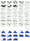 |
Fig. 1 Output summary of the optical and UV Kiwi-GA run of Farina-88 (O4 III(f)). The top part of the figure shows all used diagnostics: the observed spectra (black; vertical bars show uncertainty on each observed flux), the best fit model (dark green solid line), and the uncertainty region (light green shaded area; this area covers all model spectra of which the parameters lie within the 2σ uncertainties). The bottom part of the figure shows the fitness distribution (blue dots) of all parameters that were fitted in the optical and UV run; red vertical lines indicate the best fit value, the shaded regions indicate 1σ (orange) and 2σ (yellow) uncertainty margins. Output summaries of the other stars can be found on Zenodo. |
5 Discussion
5.1 Hertzsprung-Russell diagram
Figure 2 shows our sample stars in the Hertzsprung-Russell diagram (HRD). All sources have moved away from the zero-age main-sequence (ZAMS); at an age of 1–5 Myr, the stars are, on average, at 40–60% of their main sequence lifetime. Effective temperature and surface gravity are correlated as can be seen from the colour gradient, implying furthermore that surface gravity is correlated with age, given that stars move to lower temperatures during the main sequence.
One source, LH 114-7 (O2 III(f*)), is very hot (Teff ≈59 000 K) and lies on the blue side of the ZAMS. With BONNSAI we did not obtain evolutionary parameters for this star. While we can reproduce the combination of observed Teff, L, and v sin i well with the Brott et al. (2011) track of Mini = 40 M and vini = 538 km s–1 (see Fig. 3), the observed helium abundance and surface gravity do not match. However, we suspect that this star is a binary given its unusual combination of spectral lines: with this high temperature we obtain a good fit for He II and the highly ionised metal lines, but He I lines, absent at such high temperatures, are clearly visible in the observed spectrum. Possibly, this would affect our inference of the surface properties. Assuming that both O v λ1371 and C IV λλ1548-1551 are saturated for one of the stars and absent for the other, we estimate the light ratio of the two stars to be approximately 1:1, which would translate in a luminosity of log L/L⊙ ≈ 5.6 for either star, positioning the star near the Mini = 25 M track in Fig. 3, assuming that the temperature we inferred is approximately correct. Although beyond the scope of this paper, it might be interesting to investigate further the evolutionary history of this system.
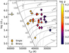 |
Fig. 2 Our sample stars in the HRD. Presumed single stars are indicated with diamonds; suspected binaries with circles. The colour of each marker corresponds to its surface gravity, where lighter colours correspond to higher values. As expected, a trend in surface gravity is seen as a function of temperature and age, which are correlated: more evolved stars are cooler and have lower surface gravity, implying a larger radius. In the background, evolutionary tracks (solid lines) and isochrones (dashed lines) of the grids of Brott et al. (2011) and Köhler et al. (2015) are shown (initial rotation rates: 170–200 km s–1). The vertical solid line indicates the position of the ZAMS; numbers on the left of the ZAMS refer to the initial mass of each model. The figure shows that our sample stars have an initial mass in the range ≈25–75 M , and an age of 1–5 Myr. One source, LH 114-7, lies on the blue side of the ZAMS; we cannot estimate its age and mass from this HRD (but see Fig. 3). |
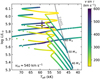 |
Fig. 3 HRD position of LH 114-7 compared to evolutionary tracks of the grid of Brott et al. (2011) with an initial rotation of 540 km s–1. Initial masses are indicated next to the ZAMS (grey solid line); the ZAMS of the track with the lower luminosity tracks fall off the scale of this plot; the initial masses of these models are, in order of decreasing luminosity, 35, 30 and 25 M⊙. Colour coding indicates v sin i, both for the tracks and the observation. The surface rotational velocities of the tracks have been multiplied by π/4, to obtain an (average) indication for v sin i. We find the best match of the observed Teff, L and v sin i of LH 114-7 to be with the Mini = 40 M⊙ track (but see text). |
 |
Fig. 4 Mass-loss rates (top panel) and modified wind momentum (bottom panel) derived from the optical+UV analysis of the single stars (green diamonds) and binaries (blue circles), compared to the mass-loss predictions of Vink et al. (2001, pink dashed lines), Krtička & Kubát (2018, dark orange dashed-dotted lines), and Björklund et al. (2021, light orange dotted lines). The pink shaded region around the Vink et al. (2001) relation in the top panel indicates spread of the predicted rates due to the inclusion of stellar parameters other than luminosity (Teff and Mevol). In grey we show the LMC observations of Brands et al. (2022) and Hawcroft et al. (2024a). Most stars of our sample have mass-loss rates that are lower than the predictions of Vink et al. (2001), and higher than those of Krtička & Kubát (2018) and Björklund et al. (2021). The light blue solid lines shows the empirical relation obtained by fitting a linear relation through all points of the three samples combined; for the mass-loss rate, it shows a good agreement with the relation of Krtička & Kubát (2018), having nearly the same slope and an average offset of only ∼0.1 dex. |
5.2 Mass-loss rates
In this section, we discuss the observed mass-loss rates in the context of theoretical predictions and other observational studies of LMC stars that use the same methodology for the spectroscopic analysis. We do not address the metallicity dependence of mass loss; this topic is discussed in detail in Backs et al. (2024), who include the results of this study in their analysis.
Figure 4 shows the observed mass-loss rates and modified wind momentum ( )) as a function of luminosity, as well as theoretical predictions of Vink et al. (2001), Krtička & Kubát (2018) and Björklund et al. (2021)23,24. In the background we show the LMC mass-loss rates and wind momentum of Brands et al. (2022, stars in R136, 30 Doradus) and Hawcroft et al. (2024a, stars in other regions of 30 Doradus), which are derived using the same method25. We carry out orthogonal distance regression (ODR) fits through the observations of all three LMC samples (Brands et al. 2022, Hawcroft et al. 2024a, and this work, as shown in Fig. 4) and derive the following empirical relations:
![\log \dot{M} \ [M_\odot \mathrm{yr}^{-1}] = (-15.70\pm 0.46) + (1.65\pm 0.08) \log L/L_\odot](/articles/aa/full_html/2025/05/aa52784-24/aa52784-24-eq22.png) (9)
and
(9)
and
![\log D_\mathrm{mom} \ [\mathrm{g \ cm \ s^{-2}}] = (17.48 \pm 0.53) + (1.94 \pm 0.09) \log L/L_\odot,](/articles/aa/full_html/2025/05/aa52784-24/aa52784-24-eq23.png) (10)
for the LMC mass loss and modified wind momentum, respectively. We stress that all mass-loss rates presented here, and thus the above equations, rely on the simultaneous fit of the windstructure (clumping) parameters, and therefore need not to be ‘corrected’ for clumping, for instance, scaled by a factor
(10)
for the LMC mass loss and modified wind momentum, respectively. We stress that all mass-loss rates presented here, and thus the above equations, rely on the simultaneous fit of the windstructure (clumping) parameters, and therefore need not to be ‘corrected’ for clumping, for instance, scaled by a factor  as one could do when working with models with a smooth wind.
The observed mass-loss rates of our sample stars show a spread of ≈0.5 dex for a given luminosity (Fig. 4). The origin of this scatter lies partially in statistical uncertainties, which for the mass-loss rate typically are 0.1–0.2 dex (Table B.2). We do not know the origin of the remainder of the scatter. A mass dependence does not seem to be the cause, as the scatter is similarly present when we look at log L/L⊙ versus modified wind momentum (Fig. 4), or at Γe versus M˙ (Fig. 5). Furthermore, we find no correlation between Teff and the residuals of the best empirical fit (light blue solid line in Fig. 4), implying that also a temperature dependence cannot explain the scatter. Likely, the scatter is caused by a physical process that we do not consider in our analysis, or that we do not consider correctly. The treatment of the wind structure is a candidate for such a process and we discuss this further in Section 5.3.
Comparing our mass-loss rates and wind momentum to theoretical predictions26, we find that Vink et al. (2001) overestimate both the mass-loss rate and wind momentum, while Krtička & Kubát (2018) and Björklund et al. (2021) underestimate these quantities. The ratio between the observed and theoretical quantities for the stars in our sample is given in Table 6. The ratios show that the predictions of Krtička & Kubát (2018) best match the observed mass-loss rates, while those of Björklund et al. (2021) provide only a slightly poorer fit. The observed modified wind momenta are best reproduced by the prescription of Björklund et al. (2021).
Upon comparing the observed rates to those of Brands et al. (2022) and Hawcroft et al. (2024a), we find for our single stars rates that they are on average 0.3 dex higher in the luminosity range where these samples overlap; the rates of these authors agree well with Krtička & Kubát (2018) and Björklund et al. (2021) in this luminosity range. The reason for the discrepancy between the different samples seems to be related to the typical stellar masses of the different samples. Upon comparing the mass-loss rates of the samples as a function of ΓEdd,e rather than log L/L , we find a good agreement between the samples; see Fig. 5. The figure includes a fit to the mass-loss prescription of Bestenlehner (2020) for each of the samples. Bestenlehner (2020) describes mass loss as a function of ΓEdd,e, the transition mass-loss rate  , and the force multiplier αeff27. In the ΓEdd,e-range where our samples overlap, the best fits are nearly identical. At low luminosities the three fits differ, but for both our sample as well as that of Hawcroft et al. (2024a) in this ΓEdd,erange the best fit is an extrapolation rather than a true fit due to the lack of data. The best fit values for
  and αeff, for each individual sample as well as those of all samples combined, can be found in Table 5.
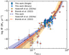 |
Fig. 5 Mass-loss rate versus Eddington factor for electron scattering for three samples of LMC O-type stars: Brands et al. (2022, red squares) Hawcroft et al. (2024a, yellow pentagons), and the sample presented in this work (green diamonds for the presumed single stars, and blue circles for the binaries). To each sample we fitted the mass-loss prescription of Bestenlehner (2020, their equation (12); see Table 5 for our best fit values). Within uncertainties the fits to the three different samples are in agreement. |
Best-fit values of the mass-loss prescription of Bestenlehner (2020) fitted to three different samples.
Mean ratios of theoretical (subscript ‘t’) to observed (subscript ‘o’) mass-loss rates and modified wind momenta.
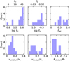 |
Fig. 6 Distribution of observed values of wind parameters for the presumed single stars in our sample for which we obtain good fits (see text). From left to right, top to bottom, we show the clumping factor, the interclump density factor, the velocity-porosity, the wind turbulence, and the onset velocity and radius of clumping. Each distribution peaks around a certain value, except for the distribution of the velocity-porosity, which is more or less flat for fvel ≳ 0.4. See also Table 7. |
5.3 Wind structure parameters
Assuming that the winds of all our stars are governed by the same wind physics, and given the inferred uncertainties on our measurements, we hypothesise to see a certain degree of structure in our results. Either, we would expect that the parameter space is only partially occupied (i.e. all parameters have a certain value), or else we would expect to find trends as a function of stellar (Teff, L) or wind ( ) parameters. In this section we investigate trends in the wind-structure properties derived for the (presumed) single stars of our sample.
Figure 6 shows the distributions of the best fit values of wind- structure parameters, and weighted mean values are listed in Table 7. The distribution of the parameters cluster around certain values: clumping factors at fcl ≈ 25–50; the interclump density at fic ≈ 0.1–0.3; the onset velocity of clumping and the wind turbulence cluster around 0.05–0.15 v∞. We find the flattest distribution for the velocity-porosity: the values range from 0.4–1.0, with the exception of one star (Sk –69°10428) for which we find fvel = 0.28 ± 0.23. It thus appears that the winds of O-type giants, bright giants and supergiants are highly clumped, with moderate to strong velocity-porosity effects. A mean interclump density factor of fic = 0.2 and a clumping factor of fcl = 33 implies that on average (for this sample) the density of the clumps is way higher than that of the surrounding medium (ρcl/ρic ≈ 200; Eqs. (4), (8) and (17) of Sundqvist & Puls 2018), but at the same time the clumps take up only a fraction of the space (fvol ≈ 0.03; Eq. (17) of Sundqvist & Puls 2018), such that 20% of the wind mass is contained in the interclump medium ((1 - fvol)fic = 0.2).
The best-fit values for the clumping onset peak around 0.05–0.15v∞; expressed in stellar radii this is around 1 R* - 1.5 R*. This is higher than what is found by Puls et al. (2006), who study the radial stratification of clumping in O-stars and infer a typical onset of clumping at 1.05 R*. Šurlan et al. (2013) found that a non-void interclump medium can hide the signature of the onset of clumping; Puls et al. (2006) assume a void interclump medium, while we assume that it is non-void. However, we do not find such degeneracy from our correlation analysis (Section 5.5), implying that this does not explain the differences between our findings and those of Puls et al. (2006).
Figure 7 shows the inferred wind-structure parameters as a function of mass-loss, and also includes the values that are obtained by Brands et al. (2022) and Hawcroft et al. (2024a); these authors also analyse optical and UV data of LMC stars using a genetic algorithm and FASTWIND, fitting the same wind- structure parameters29. Brands et al. (2022) find a tentative correlation between the mass-loss rate and several clumping parameters (~fcl, fic, fvel, vwindturb), where they infer smoother winds for stars with high mass-loss rates ( ) than for stars with lower mass-loss rates. Hawcroft et al. (2024a) cannot confirm this trend, but do infer a statistically significant correlation between effective temperature and fic and fvel. We now combine their and our data sets and compute the Kendall correlation coefficient (τk; Kendall 1938; see also our Section 5.5) to quantify possible correlations between stellar and wind parameters (Teff, L,
  ) and the wind-structure parameters (~fcl, fic, fvel, vcl,start, and vwindturb). In these tests we only consider the stars with luminosity classes I-III. We find no significant trends, with the exception of a correlation between
  and fic, where higher values of fic generally correspond to higher
  . We find τk = 0.34 with p = 0.02, indicating a positive correlation.
Despite the trend that we recover for M˙ and fic, and the fact that the wind-structure parameters are somewhat clustered in certain parts of the parameter space (Fig. 6), there is still a large scatter in the obtained values, significantly exceeding the uncertainties. First of all, this raises the question whether our diagnostic lines are sensitive enough for these properties. Can we distinguish between them, in other words, are we able to break possible degeneracies between them? The fact that the fitness distributions from our KIWI-GA runs indicate that specific combinations fit significantly better than others, suggests that we do: it implies that different diagnostics respond in a distinct manner to the different wind parameters; otherwise the distributions would not have been peaked. We analyse the KIWI-GA output in more detail by probing degeneracies between the different wind parameters in Section 5.5. We note in this context that we find no systematic differences between the wind structure parameters of the stars with higher resolution STIS data and those for which we have lower resolution COS data; neither do we find such differences between the sources for which we do or do not include the far-UV.
Assuming that our diagnostics are adequate, a possible reason for the scatter and the lack of trends could be that physical processes are manifesting that are not included in our models. For example, in addition to the small-scale, incoherent structure that is the focus of this paper, large-scale, coherent structures could affect the line profiles (e.g. Mullan 1984; Massa & Prinja 2015), for example related to magnetic fields (Sudnik & Henrichs 2016; Driessen et al. 2021). Such variations in the line profiles could affect the inferred mass-loss rates. Massa et al. (2024) quantify this effect and report that the rms intrinsic error on the mass-loss rate inferred from a single observation is 15% for O-type stars. This is an average value, Massa et al. (2024) further report that the effect is larger for lower Teff. In addition, it is also possible that the properties of the small-scale clumps are intrinsically variable. In that case, the scatter we observe could be (partially) intrinsic: depending on the time when we observe a star, the (small-scale) clumping properties observed could be different. In the context of variability it is important to realise that the optical and UV spectra considered in this study are not taken at the same time. The optical and UV spectra could therefore correspond to different states of the wind, which could make it impossible to obtain a good fit for optical and UV lines simultaneously, and possibly lead to erroneous results (Massa et al. 2024).
The scatter could also be related to the adopted parameterisation of the wind structure. It could be that this parameterisation is inadequate, that is to say, it does not adequately represent the clumpy structure of the wind – regardless of any additional physical processes that may or may not be present. If this would be the case, the result could be that the wind-structure parameters are being reduced to merely ‘fitting parameters’, which, while they may improve the fits, do not necessarily represent real physical quantities. Apart from the lack of structure in the values of the clumping parameters, also the high values of β that we derive (〈β〉 = 1.6 ± 0.6) could point to this phenomenon: possibly β is used to somehow compensate for wind-structure effects not accounted for in our models. In addition, the relatively high values we obtain for the interclump density in combination with the derived clumping factors suggest that on average a significant fraction of the material (20%) is not contained in clumps. If this is indeed true, then the current FASTWIND approach of using one NLTE solution for all the material could be difficult to justify. Verhamme et al. (2024), who study the mass loss and wind structure of a sample of B-type (super)giants, come to a similar conclusion (see their Sect. 4.5).
If the effect that the possibly inadequate wind-structure prescription has on the inferred mass-loss rates is random rather than systematic, it should be averaged out with a large enough sample size, and we would, despite large scatter, still be able to capture the overall trend in mass loss versus luminosity or ΓEdd,e. In order to investigate the validity of our clumping parameterisation further, we would need to extend our theoretical knowledge of the wind structure: ideally, we would have 3D hydrodynamical models of the wind structure, and use these to design and calibrate our 1D parameterisation30. In this context we note that the 2D radiation-hydrodynamic O-star wind models of Driessen (2022, their Fig. 8.3.) and Debnath et al. (2024) tentatively suggest that the density distribution of wind parcels resembles a Gaussian-like rather than a bi-modal distribution. A similar distribution is found from the 3D radiation-hydrodynamic simulations of Moens et al. (2022), although these authors simulate a Wolf-Rayet star wind rather than an O-star wind. These recent findings, just as the relatively high inferred interclump medium density discussed above, contradict the assumption of a two-component medium as adopted in FASTWIND, and warrant further investigation.
Mean wind-structure parameters of our O-type (super)giants.
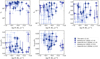 |
Fig. 7 Wind structure parameters versus mass-loss rate. Diamonds correspond to stars of our sample. We also show the samples of Brands et al. (2022, squares) and Hawcroft et al. (2024a, circles). The luminosity classes of the latter two samples are indicated with different shades. We find a positive correlation between the interclump density (fic) and the mass-loss rate, but find no correlations with any stellar parameter or mass-loss rate for the other wind-clumping parameters. |
5.4 Comparison to ‘optically-thin clumping’
In this brief section, we compare our wind structure parameterisation with an alternative, frequently used wind-structure parameterisation, namely the so called ‘microclumping’ or ‘optically-thin clumping’ approach. Here, the interclump medium is assumed to be void, while all matter is assumed to be contained in clumps that are small and rarefied enough that they stay optically thin. We test how this parameterisation would affect the derived mass-loss rates and clumping factors by refitting three semi-randomly picked stars31 in the same manner as our optical+UV runs, except for changing the clumping parameterisation to the optically-thin clumping approach; fic and fvel are no longer considered. The results are compared to our default optical+UV runs in Fig. 8. We see that the mass-loss rates that are derived with the different clumping prescriptions are in good agreement, as are the clumping factors. The similarity between the derived values suggests that if the parameterisation adopted in this paper may not be adequately describing the physics in the wind, and this causes systematic errors, the optically-thin approach suffers from similar errors.
5.5 Diagnostics and degeneracy between wind parameters
While a detailed study of the behaviour of different diagnostics is beyond the scope of this paper, it is possible to address potential degeneracies between wind parameters given our set of diagnostics by analysing the correlation plots of the best fitting models. In order to estimate the correlation between two parameters X and Y we carry out the following procedure. First, we select of each run the best fitting models (the approximately 2σ equivalent models, see Section 3.3) and make a scatter plot. The shape of this plot represents the correlation between X and Y in terms of fitness. The second step in our procedure is to quantify this shape with a correlation measure. For this we use the Kendall correlation coefficient, τk, which can assume a value between –1 and +1, where 1 is a strong negative, and +1 a strong positive correlation. The corresponding p-value, pk, reflects the significance of the obtained τk. We computed τk and pk for each parameter combination X - Y, for each star (KIWI-GA run). The third step is to count (per X - Y pair) for how many stars a significant (pk < 0.05) correlation is found per “direction” (either positive, τk > 0, or negative, τk < 0) and compute the average τk per direction. For X - Y pairs where the correlation is found for most stars and mostly in a certain direction, we conclude that there likely is a correlation between those parameters.
We applied this method to all combinations of wind parameters and as a check on whether the above method works for finding correlations, also to Teff - log g, which we know are positively correlated. Our findings are summarised in Table 8, and scatter plots as well as the τk value per star can be found on Zenodo. Table 8 shows that indeed, we recover the positive correlation between Teff and log g. Furthermore, we find a nearly equally strong (but negative) correlation between  and
and  , and between
  and β. The correlation between
  and β has been noticed previously (e.g. Puls et al. 2006; Hawcroft et al. 2021) and originates likely in optical wind lines that are formed close to the star: here both an increase in
  and a decrease in β would lead to stronger mass-loss signatures, although a decrease in β would affect the shape of the line differently. With somewhat less certainty (i.e. only for 50–70% of our stars) we find correlations between
  and log fic (negative),
  and log fvel (negative),
  and vcl,start (positive), and between log fic and fvel (negative). We stress that the fact that we find correlations between the wind parameters does not mean we are not able to break the degeneracies between these parameters. We can, up to a certain point: this is reflected in the shape of the KIWI-GA distributions (which are generally peaked rather than flat for the wind parameters), together with the uncertainties on the derived parameters, which have become larger due to the correlations (compared to the case where e.g. only the noise in the data contributed to the uncertainty). What the correlations tell us is that part of the diagnostics considered respond similarly to changes in different parameters. For example, both a higher Teff and a higher log g affect the Balmer lines similarly, and therefore we recover a correlation between the two; this is reflected by the elongated shape of the correlation plot. On the other hand, we also fit other lines (e.g. He I and He II and lines) that respond differently to an increase in Teff versus an increase in log g and therefore can break the degeneracy; this is reflected by the fact that within the elongated correlation plot there is an ‘island’ where the fittest models reside (the global minimum of the fit), namely, the best-fitting parameter combinations. We conclude our discussion on correlations by warning that the correlations presented in Table 8 apply specifically to the adopted set of diagnostics, in combination with the parameter space covered by our sample, and cannot necessarily be generalised.
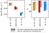 |
Fig. 8 Comparison of mass-loss rates (left) and clumping factors (right) obtained with our default optical+UV fitting method using the clumping parameterisation of Sundqvist & Puls (2018) allowing for optically thick clumps (darker shades), versus those obtained using the optically-thin clumping approach. Yellow, red, and blue bars correspond to the 1σ uncertainties of Sk -67°167, LMCe 078-1, and Sk -71°41, respectively, and the best fit values are indicated with a black dot. The values derived with the two parameterisations are in good agreement for both massloss rates and clumping factors. |
Correlations between between fitting parameters.
5.6 Terminal velocities
Figure 9 shows our terminal velocities as a function of effective temperature, together with the empirical LMC relation of Hawcroft et al. (2024b), and the theoretical predictions32 by Björklund et al. (2021), Vink & Sander (2021), and Krtička & Kubát (2018). Concerning the theoretical predictions, it is clear that none matches the empirical results. Only the prediction of Vink & Sander (2021) is similar to some extent; this relation somewhat matches the slope and absolute value of the observations, although the fit is far from perfect.
Hawcroft et al. (2024b) derive their relation based on 37 O-type stars of the ULLYSES sample, 12 of which overlap with our sample of presumed single stars. They measured the terminal velocities using the Sobolev with Exact Integration method (SEI; Lamers et al. 1987). Investigating the dependence of v∞ on both escape velocity and temperature, they found that the latter provides a tighter relation. Within uncertainties the terminal velocities of our stars are in agreement with the relation of Hawcroft et al. (2024b), with the exception of one outlier (Sk -69°104), of which the velocity exceeds the predicted value of Hawcroft et al. (2024b) with ~900 km s–1 (nearly four times the uncertainty on their relation), and three binary stars. However, the values we find are systematically higher, on average 200 km s–1 (considering only the presumed single stars, and excluding Sk 69°104). We find that the difference between both results lies in the wind turbulence velocity. This velocity is fitted both in our full spectral fit, as well as in the SEI analysis, but with the latter typically higher values are obtained. Upon comparing vmax = v∞ + vwindturb of our analysis and the SEI analysis of Hawcroft et al. (2024b), we find a good agreement without any systematic offsets. Possibly, the difference in the derived values for vwindturb is related to a different approach for computing the radial dependence of the line optical depth: in SEI this dependence is parametrised by a power law (Lamers et al. 1987; Haser et al. 1995; Sundqvist et al. 2014), while in FASTWIND this is explicitly treated in non-LTE. It could be the case that, if the optical depth structure adopted in SEI is off, a higher turbulent velocity is required in order to reproduce the observed profile.
Hawcroft et al. (2024b) also infer the terminal velocities of this sample by ‘direct measurement’, that is, by obtaining the wavelength of the bluest edge of the P-Cygni absorption showing zero flux (e.g. Prinja et al. 1990). For the 37 stars on which Hawcroft et al. (2024b) base their relation (stars with saturated profiles, labelled ‘rank i’ stars in their paper; nearly all have luminosity class I, II, or III), they find a systematic offset between the two methods, where the SEI method results in velocities that are about 200 km s–1 lower than those of the direct measurement method (green points in their Fig. 3). This implies that their direct measurements are in agreement with our detailed spectral fitting. Indeed, when comparing the values that Hawcroft et al. (2024b) obtain with this method for their class i stars, to our values, we find no systematic offset.
Overall, we confirm the tight relation of v∞ with temperature of Hawcroft et al. (2024b), but suggest a slightly modified relation for LMC stars with temperatures in the range 30 000–45 000 K:
 (11)
with v∞ in km s–1, and Teff in K. Here we assumed that the detailed FASTWIND modelling yields more reliable optical depths in the outer wind, and thus more reliable turbulent velocities than does SEI. We note that the inclusion or exclusion of N v λλ1238-1242 (see Section 5.7.1) does not affect our obtained terminal velocities significantly. Only for two of the suspected binaries we find terminal velocities that are around 450 km s–1 higher (Sk 71°19) or lower (BI 173) when N v λλ1238-1242 is included. This would not affect the fit leading to Eq. (11), for which we only considered presumed single stars. We furthermore note that our fits to the blue edge of C IV λλ1548-1551 are usually excellent, increasing the reliability of the results derived here.
(11)
with v∞ in km s–1, and Teff in K. Here we assumed that the detailed FASTWIND modelling yields more reliable optical depths in the outer wind, and thus more reliable turbulent velocities than does SEI. We note that the inclusion or exclusion of N v λλ1238-1242 (see Section 5.7.1) does not affect our obtained terminal velocities significantly. Only for two of the suspected binaries we find terminal velocities that are around 450 km s–1 higher (Sk 71°19) or lower (BI 173) when N v λλ1238-1242 is included. This would not affect the fit leading to Eq. (11), for which we only considered presumed single stars. We furthermore note that our fits to the blue edge of C IV λλ1548-1551 are usually excellent, increasing the reliability of the results derived here.
We conclude this section by inspecting the ratio v∞/vesc, where  is the effective escape velocity. For our presumed single stars we find an average ratio of 〈v∞/vesc〉 = 2.67 ± 0.25 (Fig. 10). This ratio is consistent with the typical ratio of 2.58 ± 0.20 for Galactic O-stars (Lamers et al. 1995), and with value of 〈v∞/vesc〉 = 2.4 ± 0.4 as found by Hawcroft et al. (2024b) for LMC O-stars.
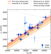 |
Fig. 9 Terminal velocities of our sample stars as a function of Teff (blue diamonds indicate single stars, with hatched symbols corresponding to supergiants; white circles indicate binaries). In the background we show the best linear ODR fit to the single star observations of our sample (red solid line, v∞ = 0.090Teff 1175), as well as the LMC relation derived by Hawcroft et al. (2024b, shown as the orange dashed line, v∞ = 0.085Teff 1150). In the background we show in grey the trends of the theoretical predictions of Björklund et al. (2021, dash-dotted line), Vink & Sander (2021, dotted line), and Krtička & Kubát (2018, solid line). We note that one source, the binary LH 114-7 (v∞ = 3425 km s–1), falls outside the range of this plot due to its high effective temperature (Teff = 59 000 K). |
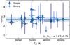 |
Fig. 10 Ratio of terminal velocity and effective escape velocity as a function of effective temperature. For our presumed single stars this ratio has a mean value of 2.67 ± 0.25 (indicated by the horizontal line and shaded area). |
5.7 CNO abundances and their uncertainties
As a by-product of our wind study we determine C, N, and O abundances for the stars in our sample. Most of the diagnostic lines from which these abundances are derived are UV wind lines. Since these lines are sensitive for many stellar and wind (structure) parameters, the derived abundances should be treated with caution. Given that our sample consists of somewhat evolved stars (Fig. 2), we expect from the CNO-cycle to see nitrogen enrichment and oxygen and carbon depletion, compared to the LMC baseline abundances. How much enrichment or depletion we expect depends on the stellar mass, rotation rate and age. Figure 11 shows the range of possible expected values per element: changes as large as 1–1.5 dex can be expected, but values close to baseline are possible too.
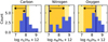 |
Fig. 11 Distribution of observed CNO abundances for our (presumed) single stars. The vertical line indicates the baseline abundances (taken from Crowther et al. 2022); the black arrows denotes the expected change in abundance when the star evolves (nitrogen enrichment, oxygen and carbon depletion), where the size of the top arrow indicates a relatively large change in abundance (corresponding to a Mini = 80 M⊙, vini = 300 km s–1 model of the Köhler et al. (2015) grid at 2.5 Myr) and the bottom arrow indicates a relatively small change (corresponding to a Mini = 40 M⊙, vini = 200 km s–1 model of the Köhler et al. (2015) grid at 2.5 Myr). The orange shaded region indicates the values that are in agreement with the expected enrichment/depletion; this range of ‘allowed values’ is based on the change in the Mini = 80 M⊙, vini = 300 km s–1 model and is extended with the average uncertainty on the observationally inferred stellar abundances (light yellow shaded region). For both carbon and oxygen, part of the stars fall outside the region of expected values. |
5.7.1 Nitrogen
For all sources, we did find indeed nitrogen enrichment compared to the LMC baseline abundance (xN = 7.03; Crowther et al. 2022; Vink et al. 2023), with a sample mean of 〈xN〉 = 8.25 ± 0.56 (see also Fig. 11). Typical uncertainties on individual values are large: on average the 1σ uncertainty range is ΔxN = 0.93 dex. For nitrogen (contrary to carbon and oxygen) we have a substantial set of optical lines available that allows us to check the results of our optical + UV analysis and make the measurement less dependent on UV wind lines. Our optical + UV values agree with the results of the optical-only runs (Fig. 12, panel a). In combination with the fact that we find enrichment for all sources we deem our inferred nitrogen abundances reliable within the derived uncertainties.
Nonetheless, we should remain cautious with the interpretation of wind line derived abundances, as a systematic error can be easily introduced when one or more other parameters regarding the wind properties are not modelled properly. For example, we did not include N v λλ1238-1242 as a diagnostic because this line is strongly affected by X-rays. Although we modelled the X-rays to the best of our ability (see Section 3.1 and Appendix D), we have indications that the implementation is not optimal. When including N v λλ1238-1242 as a diagnostic in our fits, we note that the derived nitrogen abundance is consistently higher than the nitrogen abundance derived from the optical-only fits, on average 0.33 dex (Fig. 12, panels a and b).
To investigate the cause of this discrepancy we recompute the best fit models from several optical + UV runs that include N v λλ1238-1242 as a diagnostic, adopting the nitrogen abundance of the best fit value of the optical-only run. With this lower abundance, the N v λλ1238-1242 is too weak compared to the data. It thus appears that N v λλ1238-1242 pushes towards a higher nitrogen abundance. On the other hand, a higher amount of X-rays can have the same effect on the line as an increased nitrogen abundance: experiments on three of our sample stars showed that for obtaining a good fit of N V λλ1238-1242 with the nitrogen abundance as from the optical-only fit, we need to increase the volume filling factor, fX, such that the corresponding X-ray luminosity equals log LX/L ≈ –6.5 (Fig. 12, panel c). While such values are observed at times, typically the X-ray luminosities of O-type stars are lower (e.g. Garcia & Bianchi 2004; Sana et al. 2006; Nazé 2009; Crowther et al. 2022).
The fact that we need higher X-ray luminosities than are typically observed in order to model this line could mean that our X-ray assumptions are somehow inadequate. For a better understanding of X-rays in massive-star winds and their proper implementation, it might be interesting to systematically study the effect of the different X-ray parameters by modelling N V λλ1238-1242 simultaneously with other X-ray sensitive wind lines, such as O VI λλ1031-1038. For this to be meaningful, one would need an observed (upper limit on) the X-ray flux33. The high required X-ray luminosities could also be related to the way the wind structure is implemented in FASTWIND: the same ionisation structure is adopted for both the clumps and the interclump medium, while differences between them can be expected. The models of Flores & Hillier (2021, as well as those of Flores et al. 2023) allow for different ionisation structures, which enables them to reproduce high ionization resonance transitions with an X-ray luminosity that is consistent with typical observed values.
We conclude this section by pointing out that Brands et al. (2022) do include N v λλ1238-1242 in their modelling, which could affect their inferred nitrogen abundances. However, Fig. 8 of Carneiro et al. (2016) shows that the effect might be smaller in their parameter range compared to that of our sample: for Teff ≳ 43 000 K the effect of X-rays on the N v ionisation balance is small. Most stars in the sample of Brands et al. (2022) fall in this temperature range.
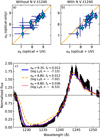 |
Fig. 12 Effect of N v λλ1238-1242 on the derived nitrogen abundance. Panels a and b compare the nitrogen abundance of the presumed single stars, derived from the optical-only runs, to that derived from the optical + UV fits in case of excluding N V λλ1238-1242 (panel a) and in case of including N V λλ1238-1242 (panel b). In the fits where N V λλ1238- 1242 is included, the nitrogen abundance is systematically higher than the values found from the optical-only runs. In panel c) we show, as an example, the N V λλ1238-1242 doublet of Sk –67°167, with the best fit model of the optical + UV run including N V λλ1238-1242 (blue solid line), a model where we altered the nitrogen abundance to the optical- only best fit value (orange dashed line), and a model where, in addition, the X-ray volume filling fraction was increased (red dotted line). The models with a high nitrogen abundance and low X-ray volume filling fraction, and a lower nitrogen abundance and higher X-ray volume filling fraction are very similar and both match the observed spectrum. |
5.7.2 Carbon and oxygen
For carbon and oxygen, we do not always find the expected depletion (Fig. 11). The sample means, 〈xC〉 = 8.03 ± 0.36 and 〈xO〉 = 8.33 ± 0.48, are close to the baseline abundances (xC = 8.01, xO = 8.40; Crowther et al. 2022; Vink et al. 2023), while on average we expect them to be somewhat lower. Uncertainties on the C and O abundances are typically large, spanning on average ΔxC = 0.68 and ΔxO = 1.05 dex, respectively, and considering this, all but three sources34 are consistent with C and O baseline abundance or lower. Nonetheless, one would still expect the mean value to be below the baseline for these elements. Unless the evolution of the carbon and oxygen enriched sources is unusual (e.g. affected by binary interaction), the somewhat high mean values and the three anomalously high abundances could imply that our inference of the C and O abundances is of poor quality. Possibly, the relatively high C and O abundances reflect limitations of our wind-structure model (see Section 5.3): this would affect the shape and strength of the wind lines, which in turn could affect the abundance determination. There is currently no way to test this hypothesis. Another possible cause for the relatively high abundances could lie in the adopted model atoms for C and O, which are not tested as extensively as the N model atom. The oxygen model, in particular, needs to be more carefully tested (Carneiro et al. 2019). Upon inspecting the line profiles (Section 4), we notice that the fits to O IV λ1340 are often poor; this could affect the abundance determination and possibly finds its origin in the model atom. Micro turbulence, for which we adopted a fixed value of vmicro = 15 km s–1 for our study, could also affect the abundance determinations. We tested the effects of our assumption by re-fitting three stars with vmicro as a free parameter: of the presumed single stars with a higher than baseline oxygen and/or carbon abundance, we picked three stars at random (Sk –67°167, LMCe 078-1, and Sk –71°41). We found best-fit values in the range vmicro = 17–21 km s–1, not too far from our original assumption, and no significant changes in abundance when varying vmicro (Fig. 13). Lastly, we point out the possibility that the high abundances that we derive reflect the limitations of our 1D models. For the abundance determination of the Sun, the use of 3D, time-dependent hydrodynamical models resulted in downward revisions of, in particular, the C, N, O, and Ne abundances (Asplund et al. 2009). Although the first steps toward 3D treatment of massive star atmospheres have been made (e.g. Moens et al. 2022; Schultz et al. 2023), it remains to be seen whether this will result in similar changes in abundance as for Solar type stars.
While at this point we cannot be certain what the true values of the abundances are, we can check whether our results, particularly the derived wind parameters, are robust against changes in abundance, in particular for stars with a high oxygen or carbon abundance. For this we look again at the results of our test where we vary vmicro, and in addition fit the same three stars, but now with fixed values of CNO abundances, where we adopt LMC baseline values. The tests shows that both Teff and the wind parameters are robust against these changes (Fig. 13). The only parameter that seems affected significantly, for one source, is fcl. Apparently in some cases, a small change in micro turbulence and/or the corresponding abundances can significantly affect the value of the clumping factor. This could explain part of the scatter we see for the clumping factor in Fig. 7. We stress that we see this only for the clumping factor (and only for one star) and that the mass-loss rate and the other wind-structure parameters have not changed significantly.
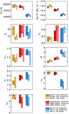 |
Fig. 13 Comparison of the results for three stars (displayed in different colors: orange for Sk -67°167, red for LMCe 078-1, and blue for Sk -71°41). We compare our default runs (darkest shade, Tables B.1 and B.2) with two different test runs: in one case we set vmicro as a free parameter (middle shade; labeled ‘vmicro’), in the other case we fix the CNO abundances to the LMC baseline values (lightest shade; labeled ‘cno’). Each bar indicates the 1σ range of parameter values, the dot indicates the best fitting model. A free vmicro does not result in significant changes in abundance. Furthermore, we see that both Teff as well as wind parameters are robust against changes in vmicro and abundance. |
6 Summary and outlook
Through an analysis of optical and UV spectroscopy, we retrieved the stellar and wind parameters of 17 (presumed) single, and 7 (likely) binaries in the LMC. All stars are part of the ULLYSES and XshootU surveys. This analysis contributes to the ultimate goal of characterising the full ULLYSES sample, aiding the construction of an empirical library of spectral templates for stars at sub-solar metallicity.
Our sample consists of O-type giants, bright giants, and supergiants. We find that these are massive (20–60 M⊙), somewhat evolved stars; with ages of 1–5 Myr, they are about halfway through their main-sequence lifetime and the nitrogen surface abundance of most stars is enhanced. Furthermore, all sample stars have strong stellar winds, with mass-loss rates ranging from ![$\log \ \dot{M} \ [\mathrm{M}_\odot~\mathrm{yr}^{-1}] = -7.2 $](/articles/aa/full_html/2025/05/aa52784-24/aa52784-24-eq54.png) to -5.6, and terminal velocities of v∞ = 1400–3400 km s–1. We studied the properties of the stellar winds in detail; in particular, we scrutinised the wind-structure parameters adopting a clumping prescription that allows for clumps to become optically thick. Our approach relies on the simultaneous fit of the wind-structure (clumping) parameters and, therefore, our mass-loss rates do not need to be ‘corrected’ for clumping; for instance, scaled by a factor
to -5.6, and terminal velocities of v∞ = 1400–3400 km s–1. We studied the properties of the stellar winds in detail; in particular, we scrutinised the wind-structure parameters adopting a clumping prescription that allows for clumps to become optically thick. Our approach relies on the simultaneous fit of the wind-structure (clumping) parameters and, therefore, our mass-loss rates do not need to be ‘corrected’ for clumping; for instance, scaled by a factor  as in sometimes done when working with models with a smooth wind. Our main findings are listed below.
The mass-loss rates that we inferred for the O-type super-giants in our sample are lower than the predicted rates of Vink et al. (2001), but higher than those of Krtička & Kubát (2018) and Björklund et al. (2021). However, in the luminosity regime covered by our sample (log L/L⊙ = 5.3–6.0), the theoretical predictions are not drastically different. Furthermore, the empirical and theoretical mass-loss rates have converged within 0.5 dex or a factor of three.
We combined our sample with the LMC samples of Hawcroft et al. (2024a) and Brands et al. (2022), both obtained using the same method as we have applied here, and present empirical
 -L and Dmom-L relations for the LMC.
We find high clumping factors of 〈fcl〉 = 33 ± 14, moderate to strong velocity-porosity effects, 〈fvel〉 = 0.6 ± 0.2, and an interclump density factor of 〈fic〉 = 0.2 ± 0.1. The latter, in combination with a clumping factor of fcl = 33, implies that with respect to the winds of our sample stars, 20% of the wind material is contained in the interclump medium.
We find a positive correlation between fic and mass loss, but no dependence of other wind-structure parameters on either mass-loss rate or stellar properties.
The scatter on empirical mass-loss rates inferred from the optical and UV spectra is larger than our typical error bars on the mass-loss rates. This also holds for the scatter on the wind-structure properties (clumping parameters). We do not know whether this scatter has a physical origin or is the consequence of systematic errors. It is possible that the parameterisation of the wind structure that we adopt is inadequate; in other words, it could be that the clumpy structure of the wind is not adequately represented. This issue warrants further investigation.
We confirm the empirical relation between Teff and v∞ inferred by Hawcroft et al. (2024b), but we notice a systematic offset between our v values (derived with FASTWIND), compared to theirs (derived with SEI). On average using SEI results in values that are 200 km s–1 lower.
We consider the nitrogen abundances that we have inferred to be reliable, but oxygen and carbon abundances are typically higher than expected. This might be related to the model atoms of carbon and oxygen or originate in 3D effects that are not currently treated in our 1D models; this warrants further investigation. The uncertain abundances do not alter our conclusions about the wind parameters, as we find that these are robust against changes in CNO abundance.
This paper comprises only a small subset of the ULLYSES stars and while we included all spectral sub-types, an expansion of the sample might give us better handles on typical mass-loss values. To this end, a future study with a larger sample, possibly also including (early) O-type dwarfs, would be valuable. In parallel to this work, Backs et al. (2024) analysed ULLYSES O- type (super)giants in the Small Magellanic Cloud (SMC; Backs et al. 2024) and combined their results with Milky Way and LMC samples (including the sample of this work) to investigate the dependence of mass-loss rates on metallicity. At log L/L⊙ = 5.75, they found  , with m ~ 1; whereas at lower luminosities, a steeper scaling of m > 2 has been inferred. Such studies of the metallicity dependence of mass loss would also benefit from expanding the analysis to larger samples, in particular, towards lower luminosities and (if possible) including galaxies with an even lower metallicity than the SMC (e.g. Telford et al. 2024; Furey et al. 2025).
In parallel to these studies, it is essential to investigate the nature of the scatter on the observed mass-loss rates and wind properties. We consider what the effects are of line variability on the inferred wind parameters and what minimum set of diagnostics is required to break degeneracies between mass-loss rate, clumping, interclump density, and velocity-porosity. Lastly, it is absolutely crucial to investigate the validity of the clumping parameterisation of the FASTWIND models, for example, with the use of 2D and 3D simulations of massive-star winds (e.g. Driessen et al. 2022; Moens et al. 2022; Debnath et al. 2024).
Data availability
Additional figures, tables, and data can be found on Zenodo: https://zenodo.org/records/15013513
Acknowledgements
This publication is part of the project ‘Massive stars in low-metallicity environments: the progenitors of massive black holes’ with project number OND1362707 of the research TOP-programme, which is (partly) financed by the Dutch Research Council (NWO). SB is furthermore supported by a grant from the Dutch Research School for Astronomy (NOVA). This work used the Dutch national e-infrastructure with the support of the SURF Cooperative using grant no. EINF-3257. AACS, VR, and RRL are supported by the Deutsche Forschungsgemeinschaft (DFG – German Research Foundation) in the form of an Emmy Noether Research Group – Project-ID 445674056 (SA4064/1-1, PI Sander). AACS is further supported by funding from the Federal Ministry of Education and Research (BMBF) and the Baden-Württemberg Ministry of Science as part of the Excellence Strategy of the German Federal and State Governments. BK gratefully acknowledges support from the Grant Agency of the Czech Republic (GACˇ R 22-34467S). The Astronomical Institute in Ondˇrejov is supported by the project RVO: 67985815. FT and FN acknowledge grant PID2022-137779OB-C41 funded by the Spanish MCIN/AEI/10.13039/501100011033. DJH acknowledges support from the STScI through grant HST-AR-16131.001-A. JS and FB acknowledge the support of the European Research Council (ERC) Horizon Europe under grant agreement number 101044048. JS further acknowledges support from Belgian Research Foundation Flanders (FWO) Odysseus program under grant number G0H9218N and FWO grant G077822N. PAC and JMB acknowledge financial support from the Science and Technology Facilities Council via research grant ST/V/000853/1 (P.I. Vik Dhillon). This research is based on observations obtained with the NASA/ESA Hubble Space Telescope, retrieved from the Mikulski Archive for Space Telescopes (MAST) at the Space Telescope Science Institute (STScI). STScI is operated by the Association of Universities for Research in Astronomy, Inc. under NASA contract NAS 5-26555.
Appendix A Photometry
The applied photometry, as well as the best fitting extinction values and the resulting absolute magnitudes, are given in Table A.1.
Photometry and extinction properties of the stars in our sample.
Appendix B Results of the combined optical and UV fits
A comparison of the observed spectra and best fit models for all stars is presented in Fig. B.1 (UV diagnostics and the main windsensitive optical lines; the C III-N III complex at 4640, He II λ4686 and Hα), and Fig. B.2 (remainder of the optical lines). The spectra are ordered by temperature. For more details, see Section 4. A detailed fit overview per star, including fitness distributions of the fitted parameters can be found on Zenodo.
The best fit parameters and associated 1σ uncertainties of the optical + UV fits can be found in Table B.1 and B.2. Table B.1 includes the helium abundance and projected surface rotation as from the optical-only fits. The complete set of parameters derived from the optical-only fit can be found on Zenodo.
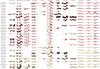 |
Fig. B.1 Normalised spectra (black) and best fit models of the UV lines, as well as the N III-C III complex, He II λ4686, and Hα for all presumed single stars (red) and binaries (orange), ordered by increasing Teff. The shaded areas indicate 2σ uncertainties. Black horizontal lines indicate the continuum; the continua of the different stars are plotted 1.5 normalised flux units apart for the UV lines, and 0.45 for the optical lines. Fig. 1 and similar plots for the other sources that can be found on Zenodo provide a more comprehensive overview per star. |
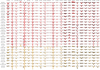 |
Fig. B.2 Same as in Fig. B.1, but for the remainder of the optical lines. The continua of the different stars are plotted 0.25 normalised flux units apart. |
Best fit values of stellar parameters, abundances, masses, and age.
Best fit values of wind parameters, Eddington factors and ionising fluxes.
Appendix C Radial velocities and multiplicity
We measure the radial velocities with a twofold purpose. First, to shift the wavelengths to rest wavelength in order to compare the data with stellar atmosphere models, and second, to reveal the presence of possible companions. For each source we have two to six epochs.
The radial velocities of the optical spectra are measured by fitting Gaussian functions to the line centres of the following lines: He II λ4200, He I λ4471, He II λ4541, He I λ4713, He I λ4921, He II λ5412, He I λ5875, N IV λ6380, O III λ5592, He II λ6406, He I λ6678, and He II λ6683. For each source, we inspected all Gaussian fits by eye, remove lines that have a bad fit, or where two diagnostics are blended35, and then adopted the mean velocity for correcting the full optical spectrum. We adopted the standard deviation on this mean as our 1σ uncertainty. We note that the barycentric velocity correction applied to the spectra released in eDR1 had the wrong sign; we corrected for this before carrying out this radial-velocity analysis. For the radial-velocity determination we used the co-added 1D spectra; we checked that this does not pose a problem for the two sources with multiple epochs; indeed, we find no radial velocity differences between the epochs. The radial velocities of the UV spectra were obtained in the normalisation process (see Section 2.3). Uncertainties were determined using the χ2-value of the fit with the iron pseudo-continuum, following the method described in Sect. 3.4 of Brands et al. (2022). We obtained radial velocities of all settings (gratings) available, also if these gratings were not used for the spectroscopic analysis.
The radial-velocity measurements for each source are presented in Table C.1. In order to identify binaries we use the statistical test described in Sana et al. (2013). We compare any two radial-velocity measurements of a given source and assess the statistical significance of rejection of the null hypothesis of constant radial velocity as following:
 (C.1)
where vi and vj are the measured radial velocities at epochs i and j, with σi and σj the 1σ uncertainties on the velocity measurements. The cut-off value of σRV > 4 as adopted by Sana et al. (2013) results in only 1 out of 1000 false positives; a less strict limit of for example σRV > 2 would result in 1 out of 20 false positives. We note that the HLSP ULLYSES spectra are corrected for heliocentric velocity, whereas the optical XshootU are corrected for the barycentric velocity; the difference between the two is very small and this thus has no significant influence on our radial-velocity comparison.
(C.1)
where vi and vj are the measured radial velocities at epochs i and j, with σi and σj the 1σ uncertainties on the velocity measurements. The cut-off value of σRV > 4 as adopted by Sana et al. (2013) results in only 1 out of 1000 false positives; a less strict limit of for example σRV > 2 would result in 1 out of 20 false positives. We note that the HLSP ULLYSES spectra are corrected for heliocentric velocity, whereas the optical XshootU are corrected for the barycentric velocity; the difference between the two is very small and this thus has no significant influence on our radial-velocity comparison.
The σRV we find for each source is shown in the last column of Table C.1. We detect radial-velocity variability at σRV > 4 for three sources: Sk -71°46, BI 173, and BI 272. Two other sources with signs of binarity in their spectra also have a relatively high σRV. The other three sources we marked as likely binaries do not show significant radial-velocity variations. Of the sources we marked as presumed single, three sources have 1 < σRV < 2. We do not see obvious signs of binarity in their spectra. We note that a radial-velocity variability analysis is not guaranteed to detect all binaries in the sample; this is true in general (binaries with small radial-velocity variations may go undetected), but even more so since the observation strategy was not optimised for binary detection. In particular, some epochs are taken very close in time (in particular the observations of the COS/G130M and COS/G160M gratings, which are usually taken right after each other), and some UV observations result in large uncertainties on the radial velocity (in particular observations obtained with FUSE and those with STIS/E230M).
Radial velocities of stars in the sample, measured in all available gratings per star.
Appendix D Wind-embedded shocks and estimating fX
For the wind-embedded shocks and resulting X-rays we use the parameterisation as implemented in FASTWIND by Carneiro et al. (2016). In this parameterisation, the X-ray properties of the wind are described by five different parameters, where the X-ray volume filling fraction fX, and the maximum jump velocity of the shocks u∞, have the most profound influence on the X-ray output; we discuss the values we adopt for these two parameters below. For the other parameters we adopt canonical values for all stars: γX = 0.75, mX = 30, and  (following Brands et al. 2022).
For the maximum jump velocity we adopt u∞ = 0.3v∞ (also following Brands et al. 2022), where we estimate v∞ prior to the KIWI-GA run by reading off the velocity at the blue edge of C IV λλ1548-1551, or in a few cases where this line is weak, from the blue edge of the Ly-α corrected N V λλ1238-1242. We want to choose the value of fX such that the typical output X-ray luminosity matches observational constraints; typically, a value of LX/L ~ 10–7 is observed (Berghoefer et al. 1997; Crowther et al. 2022). In previous work where X-rays were included in KIWI-GA fits, fX was estimated based on an observed relation with  (Kudritzki et al. 1996). With this relation fX could be predicted with an accuracy of about 1.0 dex (see Brands et al. 2022, their Appendix G.2.).
In this work, we find an improved relation between wind parameters, fX, and the X-ray luminosity. We base this relation on 1920 FASTWIND models that are randomly sampled in the O-star parameter space – including randomly sampled values of fX 36. For these models both fX as well as the output X-ray luminosity is known. In order to obtain a relation, we define a measure for the wind density, ρwind:
 (D.1)
(D.1)
Then we compare fX and ρwind of each model with the output X-ray luminosity, in other words, we fit a quadratic function of ρwind and log(LX/L) through all 1920 points, to obtain a relation that expresses fX in terms of the wind density and the desired X-ray output luminosity:
 (D.2)
with ρwind expressed in cgs-units. As we desire all our models to have an output X-ray luminosity of log(LX/L) = −7, we substitute this into Eq. (D.2) and adopt a value of fX using the following relation:
(D.2)
with ρwind expressed in cgs-units. As we desire all our models to have an output X-ray luminosity of log(LX/L) = −7, we substitute this into Eq. (D.2) and adopt a value of fX using the following relation:
 (D.3)
(D.3)
This relation is implemented in KIWI-GA and used for all our fits. Using this relation, we obtain log(LX/L) = −7 within 0.1 dex for 50% of our sample stars, within 0.25 dex for 80% of the stars, and never are we more off than 0.5 dex (see Fig. D.1). We emphasise that in the fitting process fX is not fitted, but given by Eqs. (D.1) and (D.3).
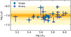 |
Fig. D.1 Adopted X-ray output luminosities as a function of total luminosity (diamonds and circles indicate single stars and binaries, respectively). Shaded areas indicate deviations of 0.1, 0.25, and 0.5 dex from log(LX/L) = –7. The adopted X-ray luminosity lies within 0.25 dex of the desired log(LX/L) = –7 for 80% of the sample stars, and within 0.5 dex for all stars. |
Appendix E Spectral type versus Teff and log g
Figure E.1 shows Teff and log g as a function of spectral sub-type. For Teff the fit to our single stars (diamonds) is in excellent agreement with the observed Galactic relations from Martins et al. (2005). For log g, we find a small offset < 0.1 dex; smaller than the typical scatter around the relation.
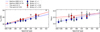 |
Fig. E.1 Relation between spectral sub-type and Teff and log g for O-type stars of luminosity class I (blue shaded markers), and II and III (red markers). |
Appendix F Comparison to literature values
Tables F.1 and F.2 contain an overview of literature values of Teff and  for our sample stars. The tables also include values for fcl in case a value was either adopted or fitted,
  (assuming fcl = 1 in case clumping was not considered), and a brief description of the methodology of each analysis. We only included analyses in which both mass-loss rate and effective temperature were derived (for LH 114-7 there were no such studies). Few stars from our sample are analysed before in as much detail as we do in this paper. Most studies use spectral type to determine Teff, several quantitative spectroscopy (but not always including UV); for the determination of
  most studies use spectroscopy, except for one, which derives its
  from the observed mid-IR excess (i.e. photometry; Massey et al. 2017). Quantitative combined optical and UV spectroscopy was only carried out for W61-28-23 (Massey et al. 2005), Sk –67°5 (Alkousa et al. 2025), Sk –71°46 (Ramachandran et al. 2018a), Sk –71°41 (Ramachandran et al. 2018b), Sk –66°171 (Sander et al. 2024, Alkousa et al. 2025) and Sk –69°50 (Sander et al. 2024)37.
In Fig. F.1 a comparison of Teff,  and
and  is shown. For stars where clumping was considered (i.e. a clumping factor was either adopted or fitted) we compare
  directly, for the other stars we compare
  . Considering typical uncertainties on the derived values (indicated by the horizontal bar in the lower right corner of the
  -subplot of Fig. F.1) and the systematic uncertainty that can be expected when analysing O-star spectra with different codes and methods (indicated by the shaded areas in Fig. F.1; see Sander et al. 2024) the values of
  agree rather well. In particular the values derived by Bestenlehner et al. (2025) agree well with ours, while their M˙ analysis does not rely on UV line profile fitting (only for determination of v∞) and their analysis is largely automated, allowing them to analyse the full ULLYSES sample. Two outliers in the
  -plot are Sk -67°5 and Sk -71°46, for which (Bestenlehner et al. 2025) and (Ramachandran et al. 2018a), respectively, find way higher mass-loss rates than we do. For Sk -67°5 the emission strength of Hα is overestimated in the best fitting model of (Bestenlehner et al. 2025), though He II λ4686 is too deep in absorption. In our analysis the emission strength of Hα matches better, as do the UV lines in our case, but the match with He II λ4686 is poor too. Considering the position of Sk -67°5 in the log
  -log L/L⊙ plot (Fig. 4) and the fit to Hα, it seems that our value for
  is more likely for this star. For Sk -71°46 Ramachandran et al. (2018a) find a mass-loss rate way higher than ours when adopting fcl = 10, though they also derive a second value assuming fcl = 20: in that case the mass-loss rates we derive are in agreement (we find
  for this source). Two more stars lie (just) outside the uncertainty range of Sander et al. (2024). For Sk -71°41 Ramachandran et al. (2018b) find a higher rate: looking at the fits we notice that their their model predicts a too strong Si IV λλ1394-1402, and has a poor fit to Hα. However, we also notice that ours and their Hα data are very different: in our data Hα is in emission, in theirs strongly in absorption. Sk -67°5 also falls just outside of the uncertainty range of Sander et al. (2024) and was analysed by Alkousa et al. (2025). Their fit is rather good, as is ours; possibly the differences arise in differing assumptions regarding the wind structure. For the analyses that do not consider clumping we compare
  and find good agreement for
  , while for
  the literature values are typically higher. With one exception, these studies do not employ UV wind lines and therefore may only have been able to derive an upper limit on the mass-loss rate.
The last panel in Fig. F.1 shows a comparison of the effective temperatures. The agreement is rather good, especially for temperatures below 40000 K. At higher temperatures, the points of Bestenlehner et al. (2025) stand out, being all significantly higher than the values we find, in the most extreme case the difference exceeds 13000 K. In concerns the sources W61-28-23, ST 92-4-18, Farina-88, and Sk -67°69. For the latter three, the models of Bestenlehner et al. (2025) predict N V λλ4604-4620 lines where these are not visible in the data, implying that these models overestimate the temperature. An explanation for this is that the normalisation around these lines is not always good as they lie close to He II λ4686, causing the pipeline of Bestenlehner et al. (2025) to decrease the weight of the data at these wavelengths. This way, the N V λλ4604-4620 lines hardly contributes to the χ2 value and the temperature can be overestimated. For W61-28-23 the N V λλ4604-4620 lines do fit well for Bestenlehner et al. (2025), where in our fit they are slightly too weak, implying that the higher temperature of Bestenlehner et al. (2025) might be more probable for this star. We conclude this section by stressing that Bestenlehner et al. (2025) do report uncertainties on their derived parameters, and that the Teff uncertainties are, as expected, rather large when too few lines were available for Teff constraints. For example, the lower 1σ uncertainty on the Teff of Farina-88 was 11700 K, meaning that within uncertainties our Teff and theirs are actually in agreement.
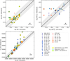 |
Fig. F.1 Values of |


References
- Abdul-Masih, M., Sana, H., Hawcroft, C., et al. 2021, A&A, 651, A96 [NASA ADS] [CrossRef] [EDP Sciences] [Google Scholar]
- Alkousa, T., Crowther, P. A., Bestenlehner, J. M., et al. 2025, A&A, submitted [Google Scholar]
- Almeida, L. A., Sana, H., Taylor, W., et al. 2017, A&A, 598, A84 [NASA ADS] [CrossRef] [EDP Sciences] [Google Scholar]
- Ardeberg, A., Brunet, J. P., Maurice, E., & Prevot, L. 1972, A&AS, 6, 249 [NASA ADS] [Google Scholar]
- Asplund, M., Grevesse, N., Sauval, A. J., & Scott, P. 2009, ARA&A, 47, 481 [NASA ADS] [CrossRef] [Google Scholar]
- Backs, F., Brands, S. A., de Koter, A., et al. 2024, A&A, 692, A88 [NASA ADS] [CrossRef] [EDP Sciences] [Google Scholar]
- Berghoefer, T. W., Schmitt, J. H. M. M., Danner, R., & Cassinelli, J. P. 1997, A&A, 322, 167 [Google Scholar]
- Bestenlehner, J. M. 2020, MNRAS, 493, 3938 [Google Scholar]
- Bestenlehner, J. M., Gräfener, G., Vink, J. S., et al. 2014, A&A, 570, A38 [NASA ADS] [CrossRef] [EDP Sciences] [Google Scholar]
- Bestenlehner, J. M., Crowther, P. A., Hawcroft, C., et al. 2025, A&A, 695, A198 [NASA ADS] [CrossRef] [EDP Sciences] [Google Scholar]
- Björklund, R., Sundqvist, J. O., Puls, J., & Najarro, F. 2021, A&A, 648, A36 [EDP Sciences] [Google Scholar]
- Brands, S. A., de Koter, A., Bestenlehner, J. M., et al. 2022, A&A, 663, A36 [Google Scholar]
- Brott, I., de Mink, S. E., Cantiello, M., et al. 2011, A&A, 530, A115 [NASA ADS] [CrossRef] [EDP Sciences] [Google Scholar]
- Burbidge, E. M., Burbidge, G. R., Fowler, W. A., & Hoyle, F. 1957, Rev. Mod. Phys., 29, 547 [NASA ADS] [CrossRef] [Google Scholar]
- Cantiello, M., Langer, N., Brott, I., et al. 2009, A&A, 499, 279 [NASA ADS] [CrossRef] [EDP Sciences] [Google Scholar]
- Carneiro, L. P., Puls, J., Sundqvist, J. O., & Hoffmann, T. L. 2016, A&A, 590, A88 [NASA ADS] [CrossRef] [EDP Sciences] [Google Scholar]
- Carneiro, L. P., Puls, J., Hoffmann, T. L., Holgado, G., & Simón-Díaz, S. 2019, A&A, 623, A3 [NASA ADS] [CrossRef] [EDP Sciences] [Google Scholar]
- Cioni, M. R. L., Clementini, G., Girardi, L., et al. 2011, A&A, 527, A116 [CrossRef] [EDP Sciences] [Google Scholar]
- Conti, P. S., Garmany, C. D., & Massey, P. 1986, AJ, 92, 48 [NASA ADS] [CrossRef] [Google Scholar]
- Crowther, P. A. 2024, in IAU Symposium, 361, eds. Mackey, J., Vink, J. S., & St-Louis, N., 15 [Google Scholar]
- Crowther, P. A., Hillier, D. J., Evans, C. J., et al. 2002, ApJ, 579, 774 [Google Scholar]
- Crowther, P. A., Broos, P. S., Townsley, L. K., et al. 2022, MNRAS, 515, 4130 [NASA ADS] [CrossRef] [Google Scholar]
- Cutri, R. M., Skrutskie, M. F., van Dyk, S., et al. 2003, VizieR Online Data Catalog: II/246 [Google Scholar]
- Cutri, R. M., Skrutskie, M. F., van Dyk, S., et al. 2012, VizieR Online Data Catalog: II/281 [Google Scholar]
- David-Uraz, A., Owocki, S. P., Wade, G. A., Sundqvist, J. O., & Kee, N. D. 2017, MNRAS, 470, 3672 [NASA ADS] [CrossRef] [Google Scholar]
- Debnath, D., Sundqvist, J. O., Moens, N., et al. 2024, A&A, 684, A177 [NASA ADS] [CrossRef] [EDP Sciences] [Google Scholar]
- Driessen, F. 2022, PhD thesis, Arenberg Doctoral School, Faculty of Science, KU Leuven, Belgium [Google Scholar]
- Driessen, F. A., Kee, N. D., & Sundqvist, J. O. 2021, A&A, 656, A131 [NASA ADS] [CrossRef] [EDP Sciences] [Google Scholar]
- Driessen, F. A., Sundqvist, J. O., & Dagore, A. 2022, A&A, 663, A40 [NASA ADS] [CrossRef] [EDP Sciences] [Google Scholar]
- ElMellah, I., Sundqvist, J. O., & Keppens, R. 2018, MNRAS, 475, 3240 [Google Scholar]
- Evans, C. J., Lennon, D. J., Smartt, S. J., & Trundle, C. 2006, A&A, 456, 623 [CrossRef] [EDP Sciences] [Google Scholar]
- Evans, C. J., Taylor, W. D., Hénault-Brunet, V., et al. 2011, A&A, 530, A108 [NASA ADS] [CrossRef] [EDP Sciences] [Google Scholar]
- Fariña, C., Bosch, G. L., Morrell, N. I., Barbá, R. H., & Walborn, N. R. 2009, AJ, 138, 510 [CrossRef] [Google Scholar]
- Feldmeier, A., Puls, J., & Pauldrach, A. W. A. 1997, A&A, 322, 878 [NASA ADS] [Google Scholar]
- Fitzpatrick, E. L. 1988, ApJ, 335, 703 [NASA ADS] [CrossRef] [Google Scholar]
- Fitzpatrick, E. L. 1999, PASP, 111, 63 [Google Scholar]
- Fitzpatrick, E. L., & Massa, D. 2005, AJ, 130, 1127 [NASA ADS] [CrossRef] [Google Scholar]
- Flores, B. L., & Hillier, D. J. 2021, MNRAS, 504, 311 [CrossRef] [Google Scholar]
- Flores, B. L., Hillier, D. J., & Dessart, L. 2023, MNRAS, 518, 5001 [Google Scholar]
- Fullerton, A. W., Crowther, P. A., De Marco, O., et al. 2000, ApJ, 538, L43 [Google Scholar]
- Fullerton, A. W., Massa, D. L., & Prinja, R. K. 2006, ApJ, 637, 1025 [Google Scholar]
- Furey, C., Telford, O. G., de Koter, A., et al. 2025, A&A, in press, https://doi.org/10.1051/0004-6361/202453128 [Google Scholar]
- Garcia, M., & Bianchi, L. 2004, ApJ, 606, 497 [NASA ADS] [CrossRef] [Google Scholar]
- Garmany, C. D., & Walborn, N. R. 1987, PASP, 99, 240 [NASA ADS] [CrossRef] [Google Scholar]
- Geen, S., Rosdahl, J., Blaizot, J., Devriendt, J., & Slyz, A. 2015, MNRAS, 448, 3248 [Google Scholar]
- Georgiev, L. N., & Koenigsberger, G. 2004, A&A, 423, 267 [NASA ADS] [CrossRef] [EDP Sciences] [Google Scholar]
- Goldoni, P. 2011, Astron. Nachr., 332, 227 [NASA ADS] [CrossRef] [Google Scholar]
- Graczyk, D., Soszyński, I., Poleski, R., et al. 2011, Acta Astron., 61, 103 [Google Scholar]
- Grinberg, V., Leutenegger, M. A., Hell, N., et al. 2015, A&A, 576, A117 [NASA ADS] [CrossRef] [EDP Sciences] [Google Scholar]
- Hamann, W. R., & Gräfener, G. 2004, A&A, 427, 697 [NASA ADS] [CrossRef] [EDP Sciences] [Google Scholar]
- Haser, S. M., Lennon, D. J., Kudritzki, R. P., et al. 1995, A&A, 295, 136 [NASA ADS] [Google Scholar]
- Hawcroft, C., Sana, H., Mahy, L., et al. 2021, A&A, 655, A67 [NASA ADS] [CrossRef] [EDP Sciences] [Google Scholar]
- Hawcroft, C., Mahy, L., Sana, H., et al. 2024a, A&A, 690, A126 [NASA ADS] [CrossRef] [EDP Sciences] [Google Scholar]
- Hawcroft, C., Sana, H., Mahy, L., et al. 2024b, A&A, 688, A105 [NASA ADS] [CrossRef] [EDP Sciences] [Google Scholar]
- Hillier, D. J. 2020, Galaxies, 8, 60 [NASA ADS] [CrossRef] [Google Scholar]
- Hillier, D. J., & Miller, D. L. 1998, ApJ, 496, 407 [NASA ADS] [CrossRef] [Google Scholar]
- Hillier, D. J., Kudritzki, R. P., Pauldrach, A. W., et al. 1993, A&A, 276, 117 [NASA ADS] [Google Scholar]
- Hopkins, P. F., Quataert, E., & Murray, N. 2011, MNRAS, 417, 950 [NASA ADS] [CrossRef] [Google Scholar]
- Isserstedt, J. 1975, A&AS, 19, 259 [NASA ADS] [Google Scholar]
- Isserstedt, J. 1979, A&AS, 38, 239 [NASA ADS] [Google Scholar]
- Isserstedt, J. 1982, A&AS, 50, 7 [NASA ADS] [Google Scholar]
- Jiang, Y.-F., Cantiello, M., Bildsten, L., Quataert, E., & Blaes, O. 2015, ApJ, 813, 74 [Google Scholar]
- Kahn, F. D. 1954, Bull. Astron. Inst. Netherlands, 12, 187 [NASA ADS] [Google Scholar]
- Kaper, L., Hammerschlag-Hensberge, G., & van Loon, J. T. 1993, A&A, 279, 485 [NASA ADS] [Google Scholar]
- Kaper, L., Henrichs, H. F., Nichols, J. S., et al. 1996, A&AS, 116, 257 [NASA ADS] [CrossRef] [EDP Sciences] [Google Scholar]
- Kaper, L., Henrichs, H. F., Nichols, J. S., & Telting, J. H. 1999, A&A, 344, 231 [NASA ADS] [Google Scholar]
- Kendall, M. 1938, Biometrika, 30, 81 [CrossRef] [Google Scholar]
- Kobayashi, C., Karakas, A. I., & Lugaro, M. 2020, ApJ, 900, 179 [Google Scholar]
- Köhler, K., Langer, N., de Koter, A., et al. 2015, A&A, 573, A71 [NASA ADS] [CrossRef] [EDP Sciences] [Google Scholar]
- Krtička, J., & Kubát, J. 2018, A&A, 612, A20 [NASA ADS] [CrossRef] [EDP Sciences] [Google Scholar]
- Kudritzki, R. P., Palsa, R., Feldmeier, A., Puls, J., & Pauldrach, A. W. A. 1996, in Roentgenstrahlung from the Universe, eds. Zimmermann, H. U., Trümper, J., & Yorke, H., 9 [Google Scholar]
- Lamers, H. J. G. L. M., Cerruti-Sola, M., & Perinotto, M. 1987, ApJ, 314, 726 [NASA ADS] [CrossRef] [Google Scholar]
- Lamers, H. J. G. L. M., Snow, T. P., & Lindholm, D. M. 1995, ApJ, 455, 269 [Google Scholar]
- Leitherer, C. 1988, ApJ, 334, 626 [Google Scholar]
- Leitherer, C., Robert, C., & Drissen, L. 1992, ApJ, 401, 596 [Google Scholar]
- Lobel, A., & Blomme, R. 2008, ApJ, 678, 408 [NASA ADS] [CrossRef] [Google Scholar]
- Lucy, L. B. 1982a, ApJ, 255, 278 [NASA ADS] [CrossRef] [Google Scholar]
- Lucy, L. B. 1982b, ApJ, 255, 286 [NASA ADS] [CrossRef] [Google Scholar]
- Lucy, L. B., & Solomon, P. M. 1970, ApJ, 159, 879 [Google Scholar]
- Markova, N., Puls, J., Repolust, T., & Markov, H. 2004, A&A, 413, 693 [NASA ADS] [CrossRef] [EDP Sciences] [Google Scholar]
- Martins, F., Schaerer, D., & Hillier, D. J. 2005, A&A, 436, 1049 [NASA ADS] [CrossRef] [EDP Sciences] [Google Scholar]
- Massa, D., & Prinja, R. K. 2015, ApJ, 809, 12 [NASA ADS] [CrossRef] [Google Scholar]
- Massa, D., Fullerton, A. W., Nichols, J. S., et al. 1995, ApJ, 452, L53 [NASA ADS] [Google Scholar]
- Massa, D., Fullerton, A. W., & Prinja, R. K. 2017, MNRAS, 470, 3765 [CrossRef] [Google Scholar]
- Massa, D., Prinja, R. K., & Oskinova, L. M. 2024, ApJ, 971, 166 [Google Scholar]
- Massey, P. 2002, ApJS, 141, 81 [NASA ADS] [CrossRef] [Google Scholar]
- Massey, P., Lang, C. C., Degioia-Eastwood, K., & Garmany, C. D. 1995, ApJ, 438, 188 [NASA ADS] [CrossRef] [Google Scholar]
- Massey, P., Waterhouse, E., & DeGioia-Eastwood, K. 2000, AJ, 119, 2214 [NASA ADS] [CrossRef] [Google Scholar]
- Massey, P., Puls, J., Pauldrach, A. W. A., et al. 2005, ApJ, 627, 477 [NASA ADS] [CrossRef] [Google Scholar]
- Massey, P., Zangari, A. M., Morrell, N. I., et al. 2009, ApJ, 692, 618 [Google Scholar]
- Massey, P., Neugent, K. F., & Morrell, N. 2017, ApJ, 837, 122 [NASA ADS] [CrossRef] [Google Scholar]
- Mihalas, D. 1978, Stellar atmospheres (San Francisco: W.H. Freeman) [Google Scholar]
- Moens, N., Poniatowski, L. G., Hennicker, L., et al. 2022, A&A, 665, A42 [NASA ADS] [CrossRef] [EDP Sciences] [Google Scholar]
- Moffat, A. F. J., & Robert, C. 1994, ApJ, 421, 310 [Google Scholar]
- Moffat, A. F. J., Drissen, L., Lamontagne, R., & Robert, C. 1988, ApJ, 334, 1038 [NASA ADS] [CrossRef] [Google Scholar]
- Mokiem, M. R., de Koter, A., Puls, J., et al. 2005, A&A, 441, 711 [NASA ADS] [CrossRef] [EDP Sciences] [Google Scholar]
- Mullan, D. J. 1984, ApJ, 283, 303 [NASA ADS] [CrossRef] [Google Scholar]
- Najarro, F., Hillier, D. J., Puls, J., Lanz, T., & Martins, F. 2006, A&A, 456, 659 [NASA ADS] [CrossRef] [EDP Sciences] [Google Scholar]
- Nazé, Y. 2009, A&A, 506, 1055 [NASA ADS] [CrossRef] [EDP Sciences] [Google Scholar]
- Niemela, V., & Gamen, R. 2004, New A Rev., 48, 727 [NASA ADS] [CrossRef] [Google Scholar]
- Oskinova, L. M., Hamann, W. R., & Feldmeier, A. 2007, A&A, 476, 1331 [NASA ADS] [CrossRef] [EDP Sciences] [Google Scholar]
- Owocki, S. P. 2008, in Clumping in Hot-Star Winds, eds. Hamann, W.-R., Feldmeier, A., & Oskinova, L. M., 121 [Google Scholar]
- Owocki, S. P., Castor, J. I., & Rybicki, G. B. 1988, ApJ, 335, 914 [NASA ADS] [CrossRef] [Google Scholar]
- Owocki, S. P., Sundqvist, J. O., Cohen, D. H., & Gayley, K. G. 2013, MNRAS, 429, 3379 [NASA ADS] [CrossRef] [Google Scholar]
- Parker, J. W., Garmany, C. D., Massey, P., & Walborn, N. R. 1992, AJ, 103, 1205 [NASA ADS] [CrossRef] [Google Scholar]
- Pietrzyński, G., Graczyk, D., Gallenne, A., et al. 2019, Nature, 567, 200 [Google Scholar]
- Prinja, R. K. 1988, MNRAS, 231, 21 [Google Scholar]
- Prinja, R. K., & Crowther, P. A. 1998, MNRAS, 300, 828 [NASA ADS] [CrossRef] [Google Scholar]
- Prinja, R. K., Barlow, M. J., & Howarth, I. D. 1990, ApJ, 361, 607 [NASA ADS] [CrossRef] [Google Scholar]
- Puls, J., Kudritzki, R. P., Herrero, A., et al. 1996, A&A, 305, 171 [Google Scholar]
- Puls, J., Urbaneja, M. A., Venero, R., et al. 2005, A&A, 435, 669 [NASA ADS] [CrossRef] [EDP Sciences] [Google Scholar]
- Puls, J., Markova, N., Scuderi, S., et al. 2006, A&A, 454, 625 [NASA ADS] [CrossRef] [EDP Sciences] [Google Scholar]
- Puls, J., Vink, J. S., & Najarro, F. 2008, A&A Rev., 16, 209 [NASA ADS] [CrossRef] [Google Scholar]
- Puls, J., Najarro, F., Sundqvist, J. O., & Sen, K. 2020, A&A, 642, A172 [EDP Sciences] [Google Scholar]
- Ramachandran, V., Hainich, R., Hamann, W. R., et al. 2018a, A&A, 609, A7 [NASA ADS] [CrossRef] [EDP Sciences] [Google Scholar]
- Ramachandran, V., Hamann, W. R., Hainich, R., et al. 2018b, A&A, 615, A40 [NASA ADS] [CrossRef] [EDP Sciences] [Google Scholar]
- Ramírez-Agudelo, O. H., Simón-Díaz, S., Sana, H., et al. 2013, A&A, 560, A29 [NASA ADS] [CrossRef] [EDP Sciences] [Google Scholar]
- Ramírez-Agudelo, O. H., Sana, H., de Koter, A., et al. 2017, A&A, 600, A81 [NASA ADS] [CrossRef] [EDP Sciences] [Google Scholar]
- Repolust, T., Puls, J., & Herrero, A. 2004, A&A, 415, 349 [NASA ADS] [CrossRef] [EDP Sciences] [Google Scholar]
- Rivero González, J. G., Puls, J., Massey, P., & Najarro, F. 2012a, A&A, 543, A95 [NASA ADS] [CrossRef] [EDP Sciences] [Google Scholar]
- Rivero González, J. G., Puls, J., Najarro, F., & Brott, I. 2012b, A&A, 537, A79 [NASA ADS] [CrossRef] [EDP Sciences] [Google Scholar]
- Roman-Duval, J., Fischer, W. J., Fullerton, A. W., et al. 2025, arXiv e-prints[arXiv:2504.05446] [Google Scholar]
- Rousseau, J., Martin, N., Prévot, L., et al. 1978, A&AS, 31, 243 [NASA ADS] [Google Scholar]
- Sana, H., Rauw, G., Nazé, Y., Gosset, E., & Vreux, J. M. 2006, MNRAS, 372, 661 [NASA ADS] [CrossRef] [Google Scholar]
- Sana, H., de Koter, A., de Mink, S. E., et al. 2013, A&A, 550, A107 [NASA ADS] [CrossRef] [EDP Sciences] [Google Scholar]
- Sana, H., Tramper, F., Abdul-Masih, M., et al. 2024, A&A, 688, A104 [NASA ADS] [CrossRef] [EDP Sciences] [Google Scholar]
- Sander, A. A. C., Bouret, J. C., Bernini-Peron, M., et al. 2024, A&A, 689, A30 [NASA ADS] [CrossRef] [EDP Sciences] [Google Scholar]
- Santolaya-Rey, A. E., Puls, J., & Herrero, A. 1997, A&A, 323, 488 [NASA ADS] [Google Scholar]
- Sanyal, D., Grassitelli, L., Langer, N., & Bestenlehner, J. M. 2015, A&A, 580, A20 [NASA ADS] [CrossRef] [EDP Sciences] [Google Scholar]
- Scannapieco, E., Pichon, C., Aracil, B., et al. 2006, MNRAS, 365, 615 [NASA ADS] [CrossRef] [Google Scholar]
- Schmidt-Kaler, T., Gochermann, J., Oestreicher, M. O., et al. 1999, MNRAS, 306, 279 [NASA ADS] [CrossRef] [Google Scholar]
- Schneider, F. R. N., Langer, N., de Koter, A., et al. 2014, A&A, 570, A66 [NASA ADS] [CrossRef] [EDP Sciences] [Google Scholar]
- Schneider, F. R. N., Castro, N., Fossati, L., Langer, N., & de Koter, A. 2017, A&A, 598, A60 [NASA ADS] [CrossRef] [EDP Sciences] [Google Scholar]
- Schultz, W. C., Bildsten, L., & Jiang, Y.-F. 2022, ApJ, 924, L11 [NASA ADS] [CrossRef] [Google Scholar]
- Schultz, W. C., Tsang, B. T. H., Bildsten, L., & Jiang, Y.-F. 2023, ApJ, 945, 58 [NASA ADS] [CrossRef] [Google Scholar]
- Smith, N. 2014, ARA&A, 52, 487 [NASA ADS] [CrossRef] [Google Scholar]
- Smith Neubig, M. M., & Bruhweiler, F. C. 1999, AJ, 117, 2856 [Google Scholar]
- Spitzer, L. 1978, Physical Processes in the Interstellar Medium (New York: Wiley-Interscience) [Google Scholar]
- Steiger, J. H. 1990, Multivariate Behav. Res., 25, 173 [Google Scholar]
- Steiger, J. H., & Lind, J. C. 1980, in The Annual Meeting of the Psychometric Society, Iowa City, IA [Google Scholar]
- Stevens, I. R. 1993, ApJ, 404, 281 [Google Scholar]
- Sudnik, N. P., & Henrichs, H. F. 2016, A&A, 594, A56 [NASA ADS] [CrossRef] [EDP Sciences] [Google Scholar]
- Sundqvist, J. O., & Puls, J. 2018, A&A, 619, A59 [NASA ADS] [CrossRef] [EDP Sciences] [Google Scholar]
- Sundqvist, J. O., Puls, J., & Feldmeier, A. 2010, A&A, 510, A11 [NASA ADS] [CrossRef] [EDP Sciences] [Google Scholar]
- Sundqvist, J. O., Puls, J., & Owocki, S. P. 2014, A&A, 568, A59 [NASA ADS] [CrossRef] [EDP Sciences] [Google Scholar]
- Sundqvist, J. O., Owocki, S. P., & Puls, J. 2018, A&A, 611, A17 [NASA ADS] [CrossRef] [EDP Sciences] [Google Scholar]
- Šurlan, B., Hamann, W. R., Kubát, J., Oskinova, L. M., & Feldmeier, A. 2012, A&A, 541, A37 [NASA ADS] [CrossRef] [EDP Sciences] [Google Scholar]
- Šurlan, B., Hamann, W. R., Aret, A., et al. 2013, A&A, 559, A130 [NASA ADS] [CrossRef] [EDP Sciences] [Google Scholar]
- Tchernyshyov, K., Meixner, M., Seale, J., et al. 2015, ApJ, 811, 78 [NASA ADS] [CrossRef] [Google Scholar]
- Telford, O. G., Chisholm, J., Sander, A. A. C., et al. 2024, ApJ, 974, 85 [NASA ADS] [Google Scholar]
- Tepper-García, T. 2006, MNRAS, 369, 2025 [CrossRef] [Google Scholar]
- Tepper-García, T. 2007, MNRAS, 382, 1375 [CrossRef] [Google Scholar]
- Tramper, F., Sana, H., de Koter, A., Kaper, L., & Ramírez-Agudelo, O. H. 2014, A&A, 572, A36 [NASA ADS] [CrossRef] [EDP Sciences] [Google Scholar]
- Verhamme, O., Sundqvist, J., de Koter, A., et al. 2024, A&A, 692, A91 [NASA ADS] [CrossRef] [EDP Sciences] [Google Scholar]
- Vernet, J., Dekker, H., D’Odorico, S., et al. 2011, A&A, 536, A105 [NASA ADS] [CrossRef] [EDP Sciences] [Google Scholar]
- Vink, J. S. 2022, ARA&A, 60, 203 [NASA ADS] [CrossRef] [Google Scholar]
- Vink, J. S., & Sander, A. A. C. 2021, MNRAS, 504, 2051 [NASA ADS] [CrossRef] [Google Scholar]
- Vink, J. S., de Koter, A., & Lamers, H. J. G. L. M. 2000, A&A, 362, 295 [Google Scholar]
- Vink, J. S., de Koter, A., & Lamers, H. J. G. L. M. 2001, A&A, 369, 574 [NASA ADS] [CrossRef] [EDP Sciences] [Google Scholar]
- Vink, J. S., Mehner, A., Crowther, P. A., et al. 2023, A&A, 675, A154 [NASA ADS] [CrossRef] [EDP Sciences] [Google Scholar]
- Walborn, N. R. 1977, ApJ, 215, 53 [NASA ADS] [CrossRef] [Google Scholar]
- Walborn, N. R., Fullerton, A. W., Crowther, P. A., et al. 2002a, ApJS, 141, 443 [NASA ADS] [CrossRef] [Google Scholar]
- Walborn, N. R., Howarth, I. D., Lennon, D. J., et al. 2002b, AJ, 123, 2754 [NASA ADS] [CrossRef] [Google Scholar]
- Walborn, N. R., Howarth, I. D., Evans, C. J., et al. 2010, AJ, 139, 1283 [NASA ADS] [CrossRef] [Google Scholar]
- Walborn, N. R., Sana, H., Simón-Díaz, S., et al. 2014, A&A, 564, A40 [NASA ADS] [CrossRef] [EDP Sciences] [Google Scholar]
- Waldron, W. L., & Cassinelli, J. P. 2010, ApJ, 711, L30 [Google Scholar]
- Weaver, R., McCray, R., Castor, J., Shapiro, P., & Moore, R. 1977, ApJ, 218, 377 [Google Scholar]
- Whiteoak, J. B. 1966, ApJ, 144, 305 [NASA ADS] [CrossRef] [Google Scholar]
- Zaritsky, D., Harris, J., Thompson, I. B., & Grebel, E. K. 2004, AJ, 128, 1606 [Google Scholar]
- Zsargó, J., Hillier, D. J., Bouret, J. C., et al. 2008, ApJ, 685, L149 [NASA ADS] [CrossRef] [Google Scholar]
We did not use these v sin i for any further analyses, but instead relied on the values found from the optical-only fits; see Section 3.4.
Also called Voigt function (see e.g. Mihalas 1978).
While we did use N V λλ1238-1242 for some experiments, we did not use it in our final analysis; see Section 5.7.1.
In the latest version of FASTWIND (v11; Puls et al. 2020) both explicit and background elements are treated in the co-moving frame. We do not use this version because the computation is slower and does not yet include an optically thick clumping prescription.
This is somewhat curious, as from conservation of angular momentum one would expect rotation to vary ∝ r–1, implying that the rotation is actually slower in the region where the wind lines are formed (unless the co-rotation is forced by for example a magnetic field); with the simple convolution that we use for modelling v sin i, this ‘slow down’ towards larger radii is not taken into account.
Other diagnostics are available in the FUSE range (see, e.g. Walborn et al. 2002a), but these are not included in our fitting as they are strongly affected by X-rays, blended with H2 Lyman-Werner absorption bands, or the relevant ions are not included as explicit ions in FASTWIND.

The BONNSAI web-service is available at https://www.astro.uni-bonn.de/stars/bonnsai/
The complete set of optical-only best fit values can be found on Zenodo.
For LH 114-7 we were not able to derive evolutionary parameters. Likely this star is evolved beyond the main sequence (see Section 5.1) and therefore its parameters are not covered by the grids of Brott et al. (2011) and Köhler et al. (2015).
Brands et al. (2022) notice something similar in the fits of their WNh stars, and name possible causes in their Appendix E.1.
We note that Eqs. (19) and (20) of Björklund et al. (2021) contain a typo: the double minus sign in the second terms of these equations should be read as a single minus sign (private communication with R. Björklund). In the arXiv pre-print the equations are correct.
The relation for wind momentum of Vink et al. (2000, their Eq. (15)) is semi-empirical as these authors do not predict terminal velocities but use observed values for v∞ and R*. The relation plotted in Fig. 4 is corrected for lowered  and v∞ as a result of the lower metallicity in the LMC compared to the Milky Way (Leitherer et al. 1992). Krtička & Kubát (2018) do not provide an explicit relation for the wind momentum; for Fig. 4 we computed Dmom for all the models in their LMC grid, and obtain a linear fit through these points as a function of luminosity. Björklund et al. (2021) provide a metallicity dependent relation for the wind momentum.
All analyses concern the simultaneous fitting of optical and UV spectra using FASTWIND and a genetic algorithm, adopting the clumping prescription of Sundqvist & Puls (2018).
See Brands et al. (2022) for a summary of the differences and similarities between the theoretical prescriptions considered here.
Brands et al. (2022) include a brief explanation of Bestenlehner (2020) and the physical meaning of αeff.
This star is the only presumed single star that does not follow the relation between terminal velocity and temperature of Hawcroft et al. (2024b); see Section 5.6.
With the exception that Hawcroft et al. (2024a) do not fit wind turbulence, but assume a fixed value of vwindturb = 0.1v∞ for all stars.
Such tests have been carried out in a simplified manner by Sundqvist et al. (2010), who used 1D models where the structures have been randomly re-shuffled to 3D space, to check a couple of effects.
We use the same stars as we use for our micro-turbulence/abundance tests; Section 5.7 details on how these stars were selected. We note that all three stars have a significant interclump density in the best fit optically thick models (fic = 0.09 for Sk –67°167, fic = 0.14 for LMCe 078-1, and fic = 0.25 for Sk –71°41).
See Brands et al. (2022) for a summary of the differences and similarities between the theoretical prescriptions considered here.
Apart from the X-ray prescription that we adopted for this work (Carneiro et al. 2016), another prescription is recently implemented in FASTWIND (Puls et al. 2020, partly based on an analysis by Owocki et al. 2013); this new parameterisation should be included in the study.
Parameters that were varied: fX, Teff, log g,  , yHe, v∞, vmicro, β, fcl, fic, fvel, vcl,start, vwindturb, and C, N, and O abundance; here fX was sampled in log space, with log fX ϵ [ 4, 1.2], yHe was sampled in the range yHe ϵ [0.09, 0.40], and the other parameters could assume values in the typical parameter range used for the fitting; see the fitness plots in Fig. 1 and on Zenodo.
Sk -66°171 and Sk -69°50 are special cases, which Sander et al. (2024) analysed with different stellar atmosphere codes and fitting strategies with the aim to investigate the parameter spread due to different fitting approaches. As Sander et al. (2024) provide an in depth discussion of these comparisons, and because the values of this paper are also used in their study, we do not include the values of the Sander et al. (2024)-analyses in our literature study.
All Tables
Overview of our sample: spectral types and UV observations used for spectral fitting.
Best-fit values of the mass-loss prescription of Bestenlehner (2020) fitted to three different samples.
Mean ratios of theoretical (subscript ‘t’) to observed (subscript ‘o’) mass-loss rates and modified wind momenta.
Radial velocities of stars in the sample, measured in all available gratings per star.
All Figures
|
Fig. 1 Output summary of the optical and UV Kiwi-GA run of Farina-88 (O4 III(f)). The top part of the figure shows all used diagnostics: the observed spectra (black; vertical bars show uncertainty on each observed flux), the best fit model (dark green solid line), and the uncertainty region (light green shaded area; this area covers all model spectra of which the parameters lie within the 2σ uncertainties). The bottom part of the figure shows the fitness distribution (blue dots) of all parameters that were fitted in the optical and UV run; red vertical lines indicate the best fit value, the shaded regions indicate 1σ (orange) and 2σ (yellow) uncertainty margins. Output summaries of the other stars can be found on Zenodo. |
| In the text | |
|
Fig. 2 Our sample stars in the HRD. Presumed single stars are indicated with diamonds; suspected binaries with circles. The colour of each marker corresponds to its surface gravity, where lighter colours correspond to higher values. As expected, a trend in surface gravity is seen as a function of temperature and age, which are correlated: more evolved stars are cooler and have lower surface gravity, implying a larger radius. In the background, evolutionary tracks (solid lines) and isochrones (dashed lines) of the grids of Brott et al. (2011) and Köhler et al. (2015) are shown (initial rotation rates: 170–200 km s–1). The vertical solid line indicates the position of the ZAMS; numbers on the left of the ZAMS refer to the initial mass of each model. The figure shows that our sample stars have an initial mass in the range ≈25–75 M , and an age of 1–5 Myr. One source, LH 114-7, lies on the blue side of the ZAMS; we cannot estimate its age and mass from this HRD (but see Fig. 3). |
| In the text | |
|
Fig. 3 HRD position of LH 114-7 compared to evolutionary tracks of the grid of Brott et al. (2011) with an initial rotation of 540 km s–1. Initial masses are indicated next to the ZAMS (grey solid line); the ZAMS of the track with the lower luminosity tracks fall off the scale of this plot; the initial masses of these models are, in order of decreasing luminosity, 35, 30 and 25 M⊙. Colour coding indicates v sin i, both for the tracks and the observation. The surface rotational velocities of the tracks have been multiplied by π/4, to obtain an (average) indication for v sin i. We find the best match of the observed Teff, L and v sin i of LH 114-7 to be with the Mini = 40 M⊙ track (but see text). |
| In the text | |
|
Fig. 4 Mass-loss rates (top panel) and modified wind momentum (bottom panel) derived from the optical+UV analysis of the single stars (green diamonds) and binaries (blue circles), compared to the mass-loss predictions of Vink et al. (2001, pink dashed lines), Krtička & Kubát (2018, dark orange dashed-dotted lines), and Björklund et al. (2021, light orange dotted lines). The pink shaded region around the Vink et al. (2001) relation in the top panel indicates spread of the predicted rates due to the inclusion of stellar parameters other than luminosity (Teff and Mevol). In grey we show the LMC observations of Brands et al. (2022) and Hawcroft et al. (2024a). Most stars of our sample have mass-loss rates that are lower than the predictions of Vink et al. (2001), and higher than those of Krtička & Kubát (2018) and Björklund et al. (2021). The light blue solid lines shows the empirical relation obtained by fitting a linear relation through all points of the three samples combined; for the mass-loss rate, it shows a good agreement with the relation of Krtička & Kubát (2018), having nearly the same slope and an average offset of only ∼0.1 dex. |
| In the text | |
|
Fig. 5 Mass-loss rate versus Eddington factor for electron scattering for three samples of LMC O-type stars: Brands et al. (2022, red squares) Hawcroft et al. (2024a, yellow pentagons), and the sample presented in this work (green diamonds for the presumed single stars, and blue circles for the binaries). To each sample we fitted the mass-loss prescription of Bestenlehner (2020, their equation (12); see Table 5 for our best fit values). Within uncertainties the fits to the three different samples are in agreement. |
| In the text | |
|
Fig. 6 Distribution of observed values of wind parameters for the presumed single stars in our sample for which we obtain good fits (see text). From left to right, top to bottom, we show the clumping factor, the interclump density factor, the velocity-porosity, the wind turbulence, and the onset velocity and radius of clumping. Each distribution peaks around a certain value, except for the distribution of the velocity-porosity, which is more or less flat for fvel ≳ 0.4. See also Table 7. |
| In the text | |
|
Fig. 7 Wind structure parameters versus mass-loss rate. Diamonds correspond to stars of our sample. We also show the samples of Brands et al. (2022, squares) and Hawcroft et al. (2024a, circles). The luminosity classes of the latter two samples are indicated with different shades. We find a positive correlation between the interclump density (fic) and the mass-loss rate, but find no correlations with any stellar parameter or mass-loss rate for the other wind-clumping parameters. |
| In the text | |
|
Fig. 8 Comparison of mass-loss rates (left) and clumping factors (right) obtained with our default optical+UV fitting method using the clumping parameterisation of Sundqvist & Puls (2018) allowing for optically thick clumps (darker shades), versus those obtained using the optically-thin clumping approach. Yellow, red, and blue bars correspond to the 1σ uncertainties of Sk -67°167, LMCe 078-1, and Sk -71°41, respectively, and the best fit values are indicated with a black dot. The values derived with the two parameterisations are in good agreement for both massloss rates and clumping factors. |
| In the text | |
|
Fig. 9 Terminal velocities of our sample stars as a function of Teff (blue diamonds indicate single stars, with hatched symbols corresponding to supergiants; white circles indicate binaries). In the background we show the best linear ODR fit to the single star observations of our sample (red solid line, v∞ = 0.090Teff 1175), as well as the LMC relation derived by Hawcroft et al. (2024b, shown as the orange dashed line, v∞ = 0.085Teff 1150). In the background we show in grey the trends of the theoretical predictions of Björklund et al. (2021, dash-dotted line), Vink & Sander (2021, dotted line), and Krtička & Kubát (2018, solid line). We note that one source, the binary LH 114-7 (v∞ = 3425 km s–1), falls outside the range of this plot due to its high effective temperature (Teff = 59 000 K). |
| In the text | |
|
Fig. 10 Ratio of terminal velocity and effective escape velocity as a function of effective temperature. For our presumed single stars this ratio has a mean value of 2.67 ± 0.25 (indicated by the horizontal line and shaded area). |
| In the text | |
|
Fig. 11 Distribution of observed CNO abundances for our (presumed) single stars. The vertical line indicates the baseline abundances (taken from Crowther et al. 2022); the black arrows denotes the expected change in abundance when the star evolves (nitrogen enrichment, oxygen and carbon depletion), where the size of the top arrow indicates a relatively large change in abundance (corresponding to a Mini = 80 M⊙, vini = 300 km s–1 model of the Köhler et al. (2015) grid at 2.5 Myr) and the bottom arrow indicates a relatively small change (corresponding to a Mini = 40 M⊙, vini = 200 km s–1 model of the Köhler et al. (2015) grid at 2.5 Myr). The orange shaded region indicates the values that are in agreement with the expected enrichment/depletion; this range of ‘allowed values’ is based on the change in the Mini = 80 M⊙, vini = 300 km s–1 model and is extended with the average uncertainty on the observationally inferred stellar abundances (light yellow shaded region). For both carbon and oxygen, part of the stars fall outside the region of expected values. |
| In the text | |
|
Fig. 12 Effect of N v λλ1238-1242 on the derived nitrogen abundance. Panels a and b compare the nitrogen abundance of the presumed single stars, derived from the optical-only runs, to that derived from the optical + UV fits in case of excluding N V λλ1238-1242 (panel a) and in case of including N V λλ1238-1242 (panel b). In the fits where N V λλ1238- 1242 is included, the nitrogen abundance is systematically higher than the values found from the optical-only runs. In panel c) we show, as an example, the N V λλ1238-1242 doublet of Sk –67°167, with the best fit model of the optical + UV run including N V λλ1238-1242 (blue solid line), a model where we altered the nitrogen abundance to the optical- only best fit value (orange dashed line), and a model where, in addition, the X-ray volume filling fraction was increased (red dotted line). The models with a high nitrogen abundance and low X-ray volume filling fraction, and a lower nitrogen abundance and higher X-ray volume filling fraction are very similar and both match the observed spectrum. |
| In the text | |
|
Fig. 13 Comparison of the results for three stars (displayed in different colors: orange for Sk -67°167, red for LMCe 078-1, and blue for Sk -71°41). We compare our default runs (darkest shade, Tables B.1 and B.2) with two different test runs: in one case we set vmicro as a free parameter (middle shade; labeled ‘vmicro’), in the other case we fix the CNO abundances to the LMC baseline values (lightest shade; labeled ‘cno’). Each bar indicates the 1σ range of parameter values, the dot indicates the best fitting model. A free vmicro does not result in significant changes in abundance. Furthermore, we see that both Teff as well as wind parameters are robust against changes in vmicro and abundance. |
| In the text | |
|
Fig. B.1 Normalised spectra (black) and best fit models of the UV lines, as well as the N III-C III complex, He II λ4686, and Hα for all presumed single stars (red) and binaries (orange), ordered by increasing Teff. The shaded areas indicate 2σ uncertainties. Black horizontal lines indicate the continuum; the continua of the different stars are plotted 1.5 normalised flux units apart for the UV lines, and 0.45 for the optical lines. Fig. 1 and similar plots for the other sources that can be found on Zenodo provide a more comprehensive overview per star. |
| In the text | |
|
Fig. B.2 Same as in Fig. B.1, but for the remainder of the optical lines. The continua of the different stars are plotted 0.25 normalised flux units apart. |
| In the text | |
|
Fig. D.1 Adopted X-ray output luminosities as a function of total luminosity (diamonds and circles indicate single stars and binaries, respectively). Shaded areas indicate deviations of 0.1, 0.25, and 0.5 dex from log(LX/L) = –7. The adopted X-ray luminosity lies within 0.25 dex of the desired log(LX/L) = –7 for 80% of the sample stars, and within 0.5 dex for all stars. |
| In the text | |
|
Fig. E.1 Relation between spectral sub-type and Teff and log g for O-type stars of luminosity class I (blue shaded markers), and II and III (red markers). |
| In the text | |
|
Fig. F.1 Values of |
| In the text | |
Current usage metrics show cumulative count of Article Views (full-text article views including HTML views, PDF and ePub downloads, according to the available data) and Abstracts Views on Vision4Press platform.
Data correspond to usage on the plateform after 2015. The current usage metrics is available 48-96 hours after online publication and is updated daily on week days.
Initial download of the metrics may take a while.