| Issue |
A&A
Volume 696, April 2025
|
|
|---|---|---|
| Article Number | A99 | |
| Number of page(s) | 23 | |
| Section | Interstellar and circumstellar matter | |
| DOI | https://doi.org/10.1051/0004-6361/202453441 | |
| Published online | 08 April 2025 | |
PDRs4All
XI. Detection of infrared CH+ and CH3+ rovibrational emission in the Orion Bar and disk d203-506: Evidence of chemical pumping
1
Université Paris-Saclay, CNRS, Institut d’Astrophysique Spatiale,
91405
Orsay,
France
2
Université Paris-Saclay, CNRS, Institut des Sciences Moléculaires d’Orsay,
91400
Orsay,
France
3
Instituto de Física Fundamental (CSIC),
Calle Serrano 121–123,
28006
Madrid,
Spain
4
Institut de Planétologie et d’Astrophysique de Grenoble (IPAG), Université Grenoble Alpes, CNRS,
38000
Grenoble,
France
5
Observatoire de Paris, Université PSL, Sorbonne Université, LERMA,
75014
Paris,
France
6
Leiden Observatory, Leiden University,
2300
RA
Leiden,
The Netherlands
7
Astronomy Department, University of Maryland,
College Park,
MD
20742,
USA
8
Institut de Radioastronomie Millimétrique (IRAM),
300 Rue de la Piscine,
F-38406
Saint-Martin d’Hères,
France
9
Department of Space, Earth and Environment, Chalmers University of Technology, Onsala Space Observatory,
43992
Onsala,
Sweden
10
Instituto de Astrofísica e Ciências do Espaço, Tapada da Ajuda, Edifício Leste,
2 ∘ Piso,
1349-018
Lisboa,
Portugal
11
Institut de Recherche en Astrophysique et Planétologie, Université Toulouse III – Paul Sabatier, CNRS, CNES,
9 Av. du colonel Roche,
31028
Toulouse Cedex 04,
France
12
Department of Physics & Astronomy, The University of Western Ontario,
London,
ON
N6A 3K7,
Canada
13
Institute for Earth and Space Exploration, The University of Western Ontario,
London
ON
N6A 3K7,
Canada
14
Carl Sagan Center, SETI Institute,
339 Bernardo Avenue, Suite 200,
Mountain View,
CA
94043,
USA
15
Space Telescope Science Institute,
3700 San Martin Drive,
Baltimore,
MD
21218,
USA
★ Corresponding author; This email address is being protected from spambots. You need JavaScript enabled to view it.
Received:
13
December
2024
Accepted:
11
February
2025
Abstract
Context. The methylidyne cation (CH+) and the methyl cation (CH3+) are building blocks of organic molecules in the ultraviolet (UV) irradiated gas, yet their coupled formation and excitation mechanisms mostly remain unprobed. The James Webb Space Telescope (JWST), with its high spatial resolution and good spectral resolution, provides unique access to the detection of these molecules.
Aims. Our goal is to use the first detection of CH+ and CH3+ infrared rovibrational emission in the Orion Bar and in the protoplanetary disk d203-506 to probe their formation and excitation mechanisms and constrain the physico-chemical conditions of the environment.
Methods. We used spectro-imaging acquired using both the NIRSpec and MIRI-MRS instruments on board JWST to study the infrared CH+ and CH3+ spatial distribution at very small scales (down to 0.1′′) and compared it to excited H2 emission. We studied their excitation in detail, and in the case of CH+, we compared the observed line intensities with chemical formation pumping models based on recent quantum dynamical calculations. Throughout this study, we compare the emission of these molecules in two environments: the Bar a photodissociation region – and a protoplanetary disk (d203-506), both of which are irradiated by the Trapezium cluster.
Results. We detected CH+ and CH3+ vibrationally excited emission both in the Bar and d203-506. These emissions originate from the same region as highly excited H2 (high rotational and rovibrational levels) and correlate less with the lower rotational levels of H2 (J′ < 5) or the emission of aromatic and aliphatic infrared bands. Our comparison between the Bar and d203-506 revealed that both CH+ and CH3+ excitation and/or formation are highly dependent on gas density. The excitation temperature of the observed CH+ and CH3+ rovibrational lines is around T ∼ 1500 K in the Bar and T ∼ 800 K in d203-506. Moreover, the column densities derived from the rovibrational emission are less than 0.1% of the total known (CH+) and expected (CH3+) column densities. These different results show that CH+ and CH3+ level populations strongly deviate from local thermodynamical equilibrium. The CH+ rovibrational supra-thermal emission (v = 1 and v = 2) can be explained by chemical formation pumping with excited H2 via C+ + H2* = CH+ + H. The difference in the population distribution of the H2* energy levels between the Orion Bar and d203-506 then result in different excitation temperatures. These results support a gas phase formation pathway of CH+ and CH3+ via successive hydrogen abstraction reactions. However, we do not find any evidence of CH3+ emission in the JWST spectrum, which may be explained by the fact its spectroscopic signatures could be spread in the JWST spectra. Finally, the observed CH+ intensities coupled with a chemical formation pumping model provide a diagnostic tool to trace the local density.
Conclusions. Line emission from vibrationally excited CH+ and CH3+ provides new insight into the first steps of hydrocarbon gas-phase chemistry in action. This study highlights the need for extended molecular data of detectable molecules in the interstellar medium in order to analyze the JWST observations.
Key words: astrochemistry / molecular processes / protoplanetary disks / stars: formation / photon-dominated region (PDR) / ISM: individual objects: Orion Bar
© The Authors 2025
 Open Access article, published by EDP Sciences, under the terms of the Creative Commons Attribution License (https://creativecommons.org/licenses/by/4.0), which permits unrestricted use, distribution, and reproduction in any medium, provided the original work is properly cited.
This article is published in open access under the Subscribe to Open model. This email address is being protected from spambots. You need JavaScript enabled to view it. to support open access publication.
1 Introduction
The methylidyne cation (CH+) and methyl cation  are expected to be among the first chemical building blocks of complex organic chemistry in the ultraviolet-irradiated gas (Smith 1992; Herbst 2021). In dense interstellar clouds, gas-phase ion-neutral reactions are assumed to produce the majority of detected small molecular species. The carbon ion chemistry is initiated by C+, which is particularly abundant in regions with a high UV radiation field, which leads to
  , and
, and  by consecutive hydrogen abstraction (e.g., Sternberg & Dalgarno 1995). The small molecular ions are then expected to react with several other species to produce a variety of hydrocarbons.
  can undergo dissociative recombination, producing CH or CH2, which can react again with C+ to produce molecules containing two carbons. Then, the chemistry chain unfolds. Unsaturated hydrocarbon ions reacting with small hydrocarbon molecules can result in various long-chain hydrocarbons (Herbst 2021). In addition, CH+ and
  are also expected to be at the origin of cyano, amino, and carboxy molecules when reacting with nitrogen- and oxygen-bearing species.
The emission of these molecules seems particularly enhanced in strongly irradiated environments. Indeed, to be formed, they require either a gas at high kinetic temperature (T > 400 K) or a gas with large abundances of rovibrationally excited H2 (see Eq. (2)). In these environments, intense far ultraviolet (FUV; E < 13.6 eV) radiation (G0 > 102 in Habing units, with G0 = 1 corresponding to a flux integrated between 91.2 and 240 nm of 1.6 × 10⁻³ erg cm−2 s−1, Habing 1968) can produce excited H2 via UV pumping. Thus, these molecules can be used to constrain the physical conditions of these specific regions, providing insight into star and planet formation limited by stellar feedback (Inoguchi et al. 2020). Moreover, the formation and excitation of CH+ and  result from specific physicochemical processes. In addition to constraining physical conditions, they can be used to probe UV-driven chemical processes.
The first detection of CH+ was in absorption in the diffuse interstellar medium (Douglas & Herzberg 1941). Since then, CH+ emission has been observed in various environments such as planetary nebulae (e.g., Cernicharo et al. 1997; Wesson et al. 2010), massive star-forming regions (e.g., Falgarone et al. 2010; Bruderer et al. 2010), disks (e.g., Thi et al. 2011), and galaxies (e.g, Spinoglio et al. 2012; Rangwala et al. 2014). In particular, far-infrared (FIR) pure rotational lines of CH+ have been detected in the Orion Bar, a prototypical and highly irradiated dense photodissociation region (PDR), with Herschel/Spectral and Photometric Imaging Receiver (SPIRE), Herschel/Photodetector Array Camera and Spectrometer (PACS), and Herschel/Heterodyne Instrument for the FarInfrared (HIFI) (Naylor et al. 2010; Habart et al. 2010; Nagy et al. 2013; Parikka et al. 2017; Joblin et al. 2018; Goicoechea et al. 2019). In warm gas, it is thought to be the product of the reaction
 (1)
(1)
which is largely endoergic when H2 is in its ground state (v′ = 0 and J′ = 0). This reaction becomes exoergic when H2 is vibrationally or rotationally excited (Stecher & Williams 1972; Jones et al. 1986; Hierl et al. 1997; Agúndez et al. 2010; Naylor et al. 2010; Godard & Cernicharo 2013; Zanchet et al. 2013; Nagy et al. 2013). While collisional excitation with H and H2 is possible for the lowest rotational levels of CH+, it is unlikely for the rovibrational levels due to their high upper energy levels and high critical densities. Moreover, collisional excitation of CH+ is hampered by the high reactivity of this species with both H and H2 (Black 1998). However, in warm environments, in addition to overcoming the endothermicity of the formation reaction, the internal energy of excited  can also be used to produce CH+ in an excited state. If the lifetime of the molecule is comparable to – or smaller than – the timescale on which the equilibrium level populations are set, the observed level populations may reflect the initial conditions at formation, and chemical formation pumping might be significant. Godard & Cernicharo (2013) showed that the pure rotational levels of CH+ with J ≥ 2 can be excited by chemical formation pumping during its formation.
This mechanism has been proposed to explain the rotational emission of CH+ in the Orion Bar. This was further confirmed by Faure et al. (2017), who compared chemical pumping models with observed CH+ line intensities. Their results are in agreement with Parikka et al. (2017) (resp. Goicoechea et al. 2019), who studied the spatial morphology of CH+ rotational emission lines in the Orion Bar (resp. at very large scales in the Orion Molecular Cloud, OMC-1) at the spatial resolution of Herschel (10′′ or 0.02 pc at 120 μm). These authors confirmed a correlation of CH+ with vibrationally excited  . Chemical pumping of the rovibrational levels (v = 1–0, P(1)–P(10)) of CH+ has been observed in the planetary nebula NGC7027 (Neufeld et al. 2021). This region has very similar physical conditions to the Orion Bar, with an FUV field intensity around G0 ∼ 105, a gas temperature around T ∼ 1000 K, and a density of about nH ∼ 3 × 105 cm−3.
In contrast to  has only recently been detected in space, outside the Solar System, with the James Webb Space Telescope (JWST) in the externally irradiated disk d203-506 near the Orion Bar (Berné et al. 2023; Changala et al. 2023) and in TW Hya, the nearest T Tauri star with a dusty gas-rich disk (Henning et al. 2024). Due to its lack of permanent dipole moment,
  does not have observable rotational transitions and was thus invisible to radioastronomy. It has only become detectable thanks to the unprecedented capacities of JWST that have enabled the probing of its vibrational spectrum. Because of its only recent detection and spectroscopic complexity, the formation pathway and excitation of
  remain elusive. It is hypothesized that
  is formed in the gas phase following successive reactions with H2:
 (2)
(2)
In addition, Pety et al. (2005) have proposed that the photodestruction of polycyclic aromatic hydrocarbons (PAHs) could be precursors of small hydrocarbons in PDRs. However, Cuadrado et al. (2015) showed that in highly irradiated PDRs, such as the Orion Bar, the photodestruction of PAHs is not a necessary requirement to explain the observed abundances of small hydrocarbons. Hence, in this region, the gas phase scenario is preferred. In this scenario,  would naturally be produced from CH+. Studying
  in light of CH+ is thus highly relevant. Similar to CH+, in the gas phase, chemical pumping induced by
  could excite
  as well.
Chemical pumping is a process that is expected to excite reactive radicals and molecules in warm irradiated regions. More particularly, hydrides (such as CH+, OH, OH+, and HF; Gerin et al. 2016), which are produced from a reaction with H2, are expected to be particularly sensitive to chemical pumping due to their high reactivity and the enhanced abundance of excited  in these warm and irradiated regions. Chemical pumping has already been employed to explain previous observations of CH+ (e.g., Godard & Cernicharo 2013; Neufeld et al. 2021), OH+ (e.g., van der Tak et al. 2013), and OH (e.g., Tabone et al. 2021; Zannese et al. 2024), and state-to-state reaction rate coefficients have been calculated through ab initio quantum calculation for different reactions in previous studies (Zanchet et al. 2013; Faure et al. 2017; Veselinova et al. 2021; Goicoechea & Roncero 2022). Molecular lines powered by chemical-pumping have also been proven to be a powerful diagnostic of the interstellar medium. Zannese et al. (2024) showed how the chemical-pumping excitation of OH via O + H2 in its rovibrational levels, detected in the irradiated disk d203-506, can be used to directly derive the formation rate of molecules and the local density from observed intensities. This method can apply to CH+ and
  since their formation reactions are similar to OH, as it is formed from
  .
.
In this paper, we present the first detection and analysis of vibrationally excited CH+ and  emission in the Orion Bar. This is compared to the detection in the externally irradiated disk (d203-506) located in the line of sight toward the atomic gas rim of the Bar (see Fig. 1). The data were provided by JWST as part of the program PDRs4All (Berné et al. 2022). The detection of near-infrared (NIR) and mid-infrared (MIR) lines with the JWST are highly complementary to previous studies, as the probed energy levels are very different and the angular resolution (0.1–1′′) of JWST is much better than Herschel’s (by a factor of 10–100). We were thus able to study the spatial morphology of the emission of these two species. In Sect. 2, we present the targets of interest. In Sect. 3, we present the observations obtained with JWST/Near-Infrared Spectrograph (NIRSpec) and JWST/Mid-Infrared Instrument – Medium Resolution Spectroscopy (MIRI-MRS) and the data reduction. In Sect. 4, we present the detection of CH+ and
  lines in both the Bar and d203-506. We also study the spatial morphology of their emission and compare it with different tracers in the region, such as H2 and the aromatic and aliphatic infrared bands (AIBs) emission. In Sect. 5, we analyze the excitation of CH+ and
  to understand the possible chemical routes. We thus study in detail their excitation temperature and compare the difference between the two PDR environments: the edge of a molecular cloud, the Bar, and the irradiated surface and photoevaporated wind of an irradiated protoplanetary disk, d203-506. In the rest of the paper, we qualify the second as the disk to simplify. In Sect. 5, we also compare the observations with a simple model including chemical pumping and radiative cascade. In Sect. 6, we discuss how to use this process as a simple diagnostic to derive local density and formation rate in these regions with this modeling. We also discuss the non-detection of
  and the other excitation mechanisms that could be at play in these observed transitions.
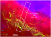 |
Fig. 1 JWST NIRCam composite image of the Orion Bar located in the Orion molecular cloud (Habart et al. 2024). Red is the 3.35 μm emission (F335M NIRCam filter), blue is the emission of Paα (F187N filter subtracted by F182M filter) and green is the emission of the H2 0–0 S(9) line at 4.70 μm (F470N filter subtracted by F480M filter). The |

2 Targets of interest
The Orion Bar, a prototypical highly irradiated PDR (for a review see Hollenbach & Tielens 1997; Wolfire et al. 2022) located in the Orion Nebula, is the closest site of ongoing massive starformation (d = 414 pc, Menten et al. 2007) and acts as a true interstellar laboratory where we can observe the non-thermal processes presented in the introduction. Indeed, this region is exposed to the intense FUV field from the Trapezium cluster, which is dominated by the O7-type star θ1 Ori C, the most massive star of the Trapezium cluster with an effective temperature Teff ≃ 40 000 K. The intense FUV radiation field incident on the ionization front (IF) of the Bar is estimated to be G0 = 2−7 × 10⁴ as derived from FUV-pumped IR-fluorescent lines (Peeters et al. 2024). This intense FUV field shapes the edge of the cloud by ionizing and photodissociating the surrounding gas composing the Orion cloud. This produces the observed PDR, subdivided into several transitions between the HII region, the atomic layer and the molecular region.
Fig. 1 shows an RGB view of the Orion Bar observed with NIRCam where both CH+ and  emission is detected. The Orion Bar, being almost edge-on, allows for the observation of the transitions between the ionized gas (in blue), the atomic gas (in red) and the H0/H2 transition, or dissociation front (DF, in green). This makes this target particularly useful to study the difference in the observed molecular characteristics, considering the variation of physico-chemical parameters between these zones. The JWST observations (Habart et al. 2024; Peeters et al. 2024) and previous observations with ALMA (Atacama Large Millimeter/submillimeter Array) (Goicoechea et al. 2016) and the Keck telescope (Habart et al. 2023) have revealed a complex geometry, where the DFs are filament-like structures at very small scales. In the field of view of MIRI-MRS and NIRSpec, we detect three dissociation fronts with thicknesses around 1′′. This complexity can be explained by a terrace-field-like structure (see Fig. 5 of Habart et al. 2024). In the rest of the study, we use the third dissociation front DF3 as a template for all DFs as it is the closest to the surface (and the observer). Indeed, differences in the attenuation of the H2 emission lines indicate that DF1 is located deeper, behind a thicker layer of atomic gas along the line of sight, and DF2 is at an intermediate position between DF1 and DF3 (Habart et al. 2024; Peeters et al. 2024).
In the field of view of MIRI-MRS and NIRSpec, we also detect a protoplanetary disk (d203-506) located along the line of sight toward the atomic layer. This disk is an almost edgeon disk seen in silhouette against the bright background. The measured radius is Rout = 98 ± 2 au and the total mass is estimated to be about 10 times the mass of Jupiter (Berné et al. 2024). The host star’s stellar mass is expected to be below 0.3 M⊙ based on kinematic studies with ALMA (Berné et al. 2024). It is unclear if d203-506 is irradiated by θ1 Ori C or θ2 Ori A (Haworth et al. 2023) as the exact location of the disk in the 3D structure is uncertain. However, the intensity of the FUV field at the surface of the disk is expected to be similar to that at the IF as determined with measurements by geometrical considerations (distance between the disk and both stars) and FUV-pumped IR-fluorescent lines (OI, H2, and CI fluorescent lines, Berné et al. 2024; Goicoechea et al. 2024). The observations by the JWST actually reveal the photoevaporative wind surrounding the edgeon disk which is bright in molecular emission (such as H2) rather than the inner disk which is hidden within it.
3 Observations and data reduction
We used MIRI-MRS and NIRSpec in the integral field unit (IFU) mode observations from the Early Release Science (ERS) program PDRs4All1: Radiative feedback from massive stars (ID1288, PIs: Berné, Habart, Peeters, Berné et al. 2022). Both MIRI-MRS and NIRSpec observations cover a 9 × 1 mosaic centered on αJ2000 = 05h 35min 20.4749s, δJ2000 = −05∘ 25′ 10.45′′. In this study, we use the full spectro-imaging cubes2 to study the spatial morphology. The MIRI-MRS data were reduced using version 1.12.5 of the JWST pipeline3, and JWST Calibration Reference Data System4 (CRDS) context jwst_1154.pmap. In addition to the standard fringe correction step, the stage 2 residual fringe correction was applied as well as a master background subtraction in stage 3 of the reduction. The 12 cubes (4 channels of 3 sub-bands each), all pointing positions combined, were stitched into a single cube (see Chown et al. 2024; Van De Putte et al. 2024, for observation parameters and data reduction details). The NIRSpec data were reduced using the JWST science pipeline (version 1.10.2.dev26+g8f690fdc) and the context jwst_1084.pmap of the Calibration References Data System (CRDS) (see Peeters et al. (2024) for observation parameters and data reduction process). We also use the MIRI-MRS and NIRSpec spectrum, in units of MJy sr−1, which were averaged on the apertures given by Berné et al. (2023) for the disk d203-506 and we used the template spectra5 from Peeters et al. (2024), Chown et al. (2024) and Van De Putte et al. (2024) for the Bar.
In this study, the emission of CH+ and H2 can be affected by extinction along the line of sight. The extinction can be neglected in d203-506 as the emission of CH+ and H2 originates from the surface of the wind. However, we need to correct this emission for extinction by the matter in the PDR and the foreground matter. To correct it, we use the R(V)-parameterized average Milky Way curve by Gordon et al. (2023), evaluated at R(V) = 5.5. In DF3, the extinction at the peak of the H2 emission is AV = 3.4, as derived by summing the extinction determined for the foreground (AV = 1.4) and that intrinsic to the atomic PDR (AV = 2) following Peeters et al. (2024) and Van De Putte et al. (2024). It is important to note that the chosen extinction curve cannot attest for the extinction of the H2 0–0 S(3) (Van De Putte et al. 2024, Zannese & Sidhu in prep). The evaluation of the proper extinction is difficult in the Orion Bar and will be discussed in Meshaka et al. (in prep). The uncertainty in the correction of extinction has a limited impact on the results of this study, considering other uncertainties.
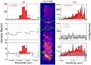 |
Fig. 2 H2 0–0 S(9) continuum subtracted map at 4.69 μm (Zannese & Sidhu in prep). The green boxes are the aperture used to extract the spectra. (Left) CH+ v = 1–0 P(5) line at 3.86 μm. (Right) |


4 Detection and spatial distribution of CH+ and CH3+ rovibrational emission
4.1 Detection of CH+
The high sensitivity and good spectral resolution of the JWST allowed for the detection of rovibrational emission of CH+ throughout the Orion Bar, in the dissociation fronts, and in the disk d203-506. Fig. 2 shows that CH+ is detected in bright H2 regions (dissociation fronts and d203-506), and is not detected, at the sensitivity of the JWST, in weaker H2 area (atomic region). These rovibrational lines were detected for the first time in NGC7027 with the NASA’s Infrared Telescope Facility (IRTF) (Neufeld et al. 2021). Except for the disk, these lines are very faint (about a hundred times fainter than H2 1–0 S(1)) so it is necessary to derive spectra from larger apertures than the size of a spaxel to increase the signal-to-noise. Line intensities are reported in Table D.1. The extinction correction of CH+ emission only increases the line intensities by a factor ∼1.3. As CH+ is detected with similar intensities in all three dissociation fronts, the intensities reported for the Bar are from DF3. The spectrum of DF3 and d203-506 in the near-infrared is presented in Fig. E.1.
We detect CH+ rovibrational lines (v = 1 → 0 (Peeters et al. 2024) and v = 2 → 1) from 3.5 to 4.4 μm with NIRSpec, up to J = 13 for v = 1 (upper energy level Eup = 7398 K) and J = 10 for v = 2 (Eup = 9743 K). The P(5) line at 3.85 μm is presented in Fig. 2. The CH+ emission from v = 1 and v = 2 is split in two branches, the R branch (below 3.62 μm) and the P branch (above 3.68 μm). The P (resp. R) branch corresponds to rovibrational lines with a change in rotational number J → J + 1 (resp. J → J − 1). Interestingly, we recover the asymmetry between the R branch and the P branch as demonstrated by Changala et al. (2021). Due to this asymmetry, the P branch is brighter than the R branch, explaining why we only detect 3 lines from the R branch. For the rest of the study, we thus focus on the P branch.
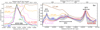 |
Fig. 3 Normalized integrated intensity profiles of the CH+ v = 1–0 P(5) line, |


4.2 Detection of CH3+
 has been first detected in the disk d203-506 (Berné et al. 2023; Changala et al. 2023). The brightest emission of
  , detected with MIRI-MRS around 7 μm, corresponds to its Q branch (Eup ≳ 2000 K) and is presented in Fig. 2. The observed emission corresponds to the out-of-plane (v2) and degenerate in-plane (v4) bending modes of the cation (Cunha de Miranda et al. 2010; Asvany et al. 2018). The initial assignment has been made possible because the pattern of successive emission lines is characteristic of the spin-statistics of a molecular carrier that would possess three equivalent non-zero-spin atoms (for example, hydrogen atoms). Moreover, the spectrum can be nicely reproduced by models using rotational constants of the order of what is expected from available calculations (Kraemer & Špirko 1991; Keceli et al. 2009). Subsequent high-level quantum calculations allowed the observed emission in d203-506 to be reproduced, and the spectroscopic assignments were confirmed by experimental measurement of the rotationally resolved photoelectron spectrum of the v2 band of
  (Changala et al. 2023).
Here, we present the first detection of this molecule in an interstellar cloud.  is detected in the three dissociation fronts as well as in d203-506, where H2 and CH+ emission is bright (see Fig. 2). Unlike CH+, the spectrum of
  around 7 μm is not spectrally resolved. As there are a lot of transitions in this wavelength range, the lines blend together and induce a molecular pseudo-continuum. As is the case for CH+, its emission in the Bar is very faint (about 50 times fainter than H2 1–0 S(1)) so we also derive the spectra from the same large aperture template. Moreover, the continuum emission at 7 μm is strong due to the presence of dust features between 7 and 9 μm, which leads to a low line-to-continuum ratio (see Fig. 2). The fringes correction in the MIRI-MRS data reduces them to about 1% and here the line-to-continuum ratio is about 4%. Hence, this complicates the analysis of the
  feature in the Bar.
4.3 Spatial distribution
The spectro-imaging of the JWST allowed us to study the spatial morphology of the Orion Bar and compare the emission of different tracers. Fig. 3 displays the normalized line intensity profile of several lines over the total IFU field of view in d203-506 (Left panel) and in the Bar (Right panel). In the Bar, each point corresponds to the intensity averaged on apertures with width of 2′′ and height varying from 0.2′′ to 1.5′′ to increase the S/N. In d203-506, we use the cut presented in Peeters et al. (2024). As seen in this figure, the emission of H2 traces the different transition fronts between the atomic layer and the molecular region (see also Zannese & Sidhu in prep for in-depth analysis of H2 emission). This emission also traces the photoevaporative wind of the disk d203-506 (Berné et al. 2024). More precisely, the rotationally excited (v′ = 0, J′ > 5) and the rovibrational emission of H2 traces the edge of the dissociation front where the temperature and FUV field are higher than further into the molecular cloud, as their excitation is driven by FUV-pumping. The lower rotational levels of H2 (J′ < 5) peak further into the cloud, where the column density is higher and the gas is still warm enough, as they are mainly excited by collisions (Van De Putte et al. 2024). The spatial separation between the lowest rotational levels of H2 and the highly excited levels is at the limit of the spatial resolution of the MIRI-MRS (0.3–1′′). The separation between the emission of H2 0–0 S(9) and H2 0–0 S(1) is visible in NIRSpec and MIRI-MRS data as highlighted in Fig. 3 and is about 0.5′′, which is barely resolved. H2 0–0 S(1) (in pink) and AIBs emission (in brown) peaks further away than H2 0–0 S(9) emission (in red) in DF3 (see also Peeters et al. 2024).
We now compare the spatial distribution of the CH+ and  emission to that of H2 lines, a very excited one, the 0–0 S(9) line – chosen as its wavelength is close to the CH+ wavelength range so it will be similarly affected by extinction – and a less excited one, the 0–0 S(1) line. Fig. 2 shows a good spatial coincidence between H2 0–0 S(9) emission and CH+ and
  emission. The intensity profiles in Fig. 3 show that CH+ peaks where H2 peaks in both d203-506 and the Bar with more spatial resolution. More precisely, CH+ emission better follows the excited H2 0–0 S(9) line emission (Eup = 10 261 K) than the less excited H2 0–0 S(1) line emission (Eup = 1015 K). This comparison between excited
  and CH+ provides a more accurate picture than the previous results (Parikka et al. 2017) which showed that CH+ rotational emission was, at the (lower) spatial resolution of Herschel, compatible with a co-spatial emission from H2 1–0 S(1). These results are in agreement with the necessity of highly excited
  to produce CH+ emission. Moreover, in both panels, it is clear that the CH+ emission profile is closer to the H2 emission than to the AIB emission at 3.3 μm and 3.4 μm. Overall, this set of results is in agreement with the gas-phase formation (and maybe excitation) of CH+ via reactions between H2 and C+ (see Eq. (1)) rather than photodestruction of dust grains.
 is too faint, or more precisely has too low line-tocontinuum ratio, in the Bar to obtain an intensity profile across the mosaic, but the left panel of Fig. 3 also shows a very good agreement with both CH+ and H2 emission in d203-506 (see also Berné et al. 2023). Fig. 2 also shows
  to be bright where H2 is bright in the Bar. This good agreement between the spatial distribution of
  and H2 is also in favor of a formation of CH+ and
  in the gas phase.
4.4 Dependence on gas density
While the normalized emission of vibrationally excited CH+ and  follows the emission of excited
  well, it is important to note that the intensity ratio of CH+ and H2 0–0 S(9) for the dissociation fronts and d203-506 is very different. Fig. 4 displays the integrated intensity ratio of CH+ P(5)/H2 0–0 S(9) and peak intensity ratio of
  as a function of H2 1–0 S(1)/H2 2–1 S(1). The H2 1–0 S(1)/H2 2–1 S(1) ratio is a tracer of density in dense highly irradiated conditions. In these conditions, collisional excitation of the H2 v′ = 1, J′ = 3 level becomes competitive when the density increases above 105 cm−3. The 1–0 S(1)/2–1 S(1) line ratio is thus expected to increase from a pure radiative cascade value (about 2) to a collisional excitation value (of the order of 10). This figure shows that for both CH+ and
  , their intensity ratio over H2 0–0 S(9) is a lot higher in d203-506 than in the Bar (a factor 10 for CH+ and
  ). In contrast, the ratio
  stays rather constant between the Bar and d203-506, with
  being slightly more enhanced (by a factor 2) at high density compared to CH+. This suggests that the excitation and/or formation of CH+ and
  depends more on gas density than the excitation of H2 0–0 S(9). This is in line with a gas-phase chemical route, as density plays a major role in the efficiency of inelastic and reactive collisions.
5 Analysis of the excitation process
The previous section showing the spatial coincidence between excited H2, CH+, and  emission gives insight into the formation pathway of these molecules and favors the gas-phase formation route. However, the spatial distribution is only one piece of the puzzle. In this section, we study in detail the excitation of the species in the Bar and in d203-506 and provide additional support for gas-phase formation and evidence for excitation at formation of at least CH+.
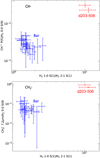 |
Fig. 4 Integrated intensity ratio of CH+ v = 1–0 P(5) over H2 0–0 S(9) (top) and peak intensity ratio of |


5.1 Rovibrational excitation temperature
5.1.1 CH+
To estimate the excitation temperature of the CH+ rovibrational transitions, we derived the absolute intensities of every line detected with sufficient signal-to-noise (S/N of at least three) and computed an excitation diagram displayed in Fig. 5. This method relies on the assumption that the emission is optically thin, which is reasonable because the column density of vibrational CH+ levels is found to be low. To derive the absolute intensities, we fitted the observed lines with a Gaussian coupled with a linear function to take into account the continuum and then integrated the Gaussian function over the wavelengths.
In the Bar, the excitation diagram of the first vibrational mode (v = 1) shows that the first two rotational levels are well populated and above J = 2, the rotational levels align along a straight line (see Fig. 5(a)). This means that the excitation of the v = 1, J ≥ 2 levels of CH+ follows a Boltzmann distribution, that is, a single temperature distribution as described by
 (3)
(3)
where Nup is the column density of the upper level of the studied transition, gup the upper-level degeneracy, N the column density, Tex the excitation temperature, Q(Tex) the partition function and kB the Boltzmann constant. We note that N corresponds to the total column density of the species only if all the levels follow Eq. (3). The excitation temperature derived in the Bar from this diagram reaches about 1500 K and reflects a supra-thermal excitation (Tex > Tgas, i.e., not only a collisional excitation). Indeed, such a high temperature is unlikely to be reached in the Bar at the dissociation front. The gas temperature derived from the H2 lines at the H0/H2 transition is similar and around T ∼ 600 K (Van De Putte et al. 2024, Zannese & Sidhu in prep and see Table 1). In addition, models from the Meudon PDR code (Le Petit et al. 2006) with consistent parameters for the Orion Bar do not predict the temperature to be higher than T ∼ 1000 K where CH+ and H2 abundances rise (Joblin et al. 2018; Zannese et al. 2023; Van De Putte et al. 2024, Meshaka et al. in prep).
We also plot the excitation diagram of the pure rotational transitions in the vibrational ground state v = 0 of CH+ (40 < Eup < 850 K) detected in the Bar with Herschel/HIFI and Herschel/PACS (Parikka et al. 2017; Joblin et al. 2018). To compare the observations of Herschel and JWST, we consider a beam dilution factor as their beam size is different. Following Joblin et al. (2018), we considered that in Herschel observations, CH+ originates from a 2′′ wide filament with infinite length, leading to beam dilution factors from 0.10 to 0.28 depending on the considered CH+ far-IR lines. Here, we see that the excitation temperature of the v = 0 levels is significantly lower than the excitation temperature of the v = 1 levels, except for the J = 0 and 1 levels within v = 1. The v = 0 levels are sub-thermally populated due to the high critical densities of the levels and high reactivity of CH+ hampering thermalization of the level via collisions. Overall, the excitation of all levels of CH+ cannot be explained by a single temperature, demonstrating a strong deviation from LTE. Another argument for the non-thermal excitation is the observed column density in the first vibrational mode v = 1 of CH+. In the Bar, we derive a column density Nvib(CH+) = (7.6 ± 2.3) × 109 cm−2. The observed column density in v = 1 is much less than in v = 0 observed by Herschel (Joblin et al. 2018, and see Fig. 5). This is supported by a comparison with predictions of standard PDR models for the Orion Bar physical parameters, which give a total column density for CH+ around N(CH+) ∼ 1014 cm−2 (Goicoechea et al. 2025). This shows that the rovibrational emission of CH+ detected with the JWST does not trace the bulk part of CH+ known to exist (predicted by models and observed by pure rotational lines) but only a very small fraction (lower than 0.1%). These results show that the excitation of CH+ in the Bar is not thermalized.
In d203-506, CH+ excitation within a vibrational level (v = 1 and v = 2) also follows a Boltzmann distribution with an excitation temperature around T = 850 K in v = 1(T = 1050 K in v = 2) which is lower than in the Bar. This temperature is similar to the gas temperature derived from H2 lines (Tgas ∼ 900 K, Berné et al. 2023, see Table 1). However, the excitation diagram shows an offset between the v = 1 and v = 2 levels. Indeed the v = 2 levels are more strongly populated than expected by extrapolating the line that fits v = 1 excitation. From this excitation diagram, we can derive a vibrational temperature between v = 1 and v = 2 using the levels v = 1, J = 7 and v = 2, J = 7 with the equation
 (4)
(4)
We measured Tvib ∼ 1300 K, which is higher than the rotational temperature Trot ∼ 900 K. It is also possible that we observe a curvature in the excitation diagram. Indeed, it seems that the high- J levels in the v = 1 have a higher excitation temperature than the low-J levels. The uncertainties in the data make it difficult to properly conclude this matter. However, once again, a unique Boltzmann distribution cannot explain the excitation of all levels of CH+ in d203-506. Even though the excitation temperature is close to the gas temperature, it is likely that, overall, levels of CH+ in the disk are also not thermalized.
Parameters derived from the analysis of the CH+ and H2 lines.
This analysis shows that the excitation temperature of CH+ is higher, and the gas kinetic temperature is lower in the Orion Bar with respect to d203-506. This result indicates that CH+ excitation in the Orion Bar is non-thermal. The different behavior of the excitation temperature highlights the difference in excitation of CH+ in these environments, which can be explained by chemical (formation) pumping. This scenario is explored in the following section.
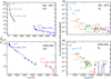 |
Fig. 5 Excitation diagram and level population of CH+ and H2 in d203-506 and in the Bar. (Left) Excitation diagram of CH+ (a) in the Bar and (c) in d203-506. (Right) Level population of H2 normalized to the total column density (see Table 1) (b) in the Bar and (d) in d203-506. The difference in H2 population distribution can explain the difference in the excitation diagram of CH+. |
5.1.2 CH3+
In order to derive the excitation temperature of  from the Q branch only (Δ J = 0), we study the evolution of the shape of the feature as shown in Fig. 6. It appears that the shorter wavelength lines in the Q branch are brighter at higher temperatures, demonstrating that the shape of the Q branch can be used to study the excitation of
  within the observed vibrational modes.
It is difficult to properly derive the integrated intensities of  because the spectrum reveals a broad feature instead of discrete lines and a very weak contrast with the dust continuum emission. Thus, we measure the difference in intensities (in MJy sr−1) between the peak and the base of selected prominent and narrow features of the Q-branch that are particularly sensitive to the temperature. This method allowed us to limit the main uncertainties in this wavelength range: fringes and continuum estimation. Indeed, in the 7 μm region, the continuum is very strong due to the rising AIBs between 7 and 9 μm which peak at 7.7 μm. This makes the slope steep and difficult to fit. Moreover, it is complicated to separate the
  molecular pseudo-continuum from the dust continuum. In DF3, the line-to-continuum ratio is very low, up to 4% at best. Hence, the challenge is to determine the dust continuum with a precision that is below 4% to be able to properly measure the
  feature. Between the peak and the base of the line, the dust continuum does not drastically vary which makes this measurement almost free of the influence of the continuum estimation.
To estimate the excitation temperature of the  emission in DF3, we use the two line ratios 7.12 μm/7.2 μm and 7.15 μm/7.2 μm. Fig. 7 shows the evolution of these ratios as a function of temperature. The modeled ratios are computed from an LTE model using the spectroscopic data from Changala et al. (2023). The measured ratio on the MIRI-MRS spectrum is overlayed in gray. The uncertainties on the measured ratio take into account the variation of the measurement considering the choice of the continuum. This figure shows that the excitation temperature is between T = 1000 K and T = 1500 K in DF3, which is much higher than the gas temperature around 600 K. This excitation temperature is similar to that of CH+. Similarly, using this method, we derive an excitation temperature around T = 700 K in d203-506, which is in agreement with the temperature derived by Changala et al. (2023) by fitting an LTE model to the observed spectrum (see Fig. E.2). As is the case for CH+, the excitation temperature of
  in DF3 is higher than the gas temperature and higher than the excitation temperature in d203-506. This is also in favor of an excitation by a non-thermal process.
Similarly to CH+, the column density of  in the Bar and the d203-506 disk are lower than what is predicted by models when using the rovibrational emission and an LTE assumption. Indeed, we estimate
  in the Bar and
  in d203-506, whereas the expected column density in the Orion Bar is
  as predicted by models at nH = 105 cm−2 and G0 = 104 (Goicoechea et al. 2025). Similarly to CH+, the observed emission of vibrationally excited
  accounts for only a very small fraction of the total abundance predicted by models.
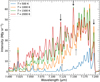 |
Fig. 6 Local thermodynamic equilibrium models of the Q branch of |


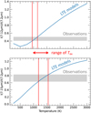 |
Fig. 7 Line ratios of |


5.2 Evidence for chemical (“formation”)-pumping of CH+
5.2.1 The model
We find the unexpected result that the excitation temperature of both CH+ and  is lower in a hotter environment (disk) than in a colder environment (DF3). The CH+ excitation due to chemical pumping has already been proposed for its ground vibrational state in the Orion Bar (Godard & Cernicharo 2013) and its v = 1 state in NGC7027 (Neufeld et al. 2021). In this section, we show that chemical pumping can naturally account for the excitation of CH+ derived from NIRSpec observations using a simple analytical model. We first assume that all the observed lines originate from a single layer and are only excited by chemical pumping by the reaction C++H2(v, J) → CH+(v′, J′)+H. To predict line intensities, we also assume that a CH+ cation produced in a given quantum state via C++H2 rapidly de-excite by a radiative cascade. We therefore neglected collisions or any other (de)excitation process such as UV or IR pumping. The critical densities of the CH+ rovibrational levels (nc ∼ 1010 cm−3) are indeed orders of magnitude higher than the expected densities in the Orion Bar or d203-506 (nH ∼ 105−107 cm−3).
The exact population distribution of CH+(v, J) following chemical pumping depends on the state-to-state rate coefficients but also on the local population densities of H2 levels. The probability to form CH+ in a given state i following C++H2 is defined as
 (5)
(5)
where xj(H2) is the level population of H2 normalized to the total population, and kj → i(T) is the state-to-state rate coefficient of the reaction ([cm3 s−1]). We use the state-to-state rate coefficients computed by Zanchet et al. (2013) with the extension of Faure et al. (2017). The available rates are for the reactions from H2 (v′ = 1, J′ = 0, 1; v′ = 2, J′ = 0) toward CH+(v = 0, 1, 2, J). Hence, we only have state-to-state molecular data for 3 levels of H2 while we have observations of more than 50 levels of H2 in the Orion Bar. In addition, we cannot compare the difference in rates between a vibrational level and a rotational level of H2 with similar energy (e.g., v′ = 0, J′ = 8 and v′ = 1, J′ = 0) as chemical pumping rates coming from highly excited rotational levels of H2 are unavailable. Hence, this study is based solely on the energy of H2 levels, without taking into account the difference between rotation and vibration. For the other levels of H2 and CH+, we used the extrapolation proposed by Neufeld et al. (2021) and we normalize it to the rate coefficient of the reaction C++ H2(v′ = 1, J′ = 0) → CH+(v = 1, J = 0) + H. New quantum calculations are needed to check the validity of this extrapolation. The dependence of these chemical pumping rates on H2 levels and temperature are presented in Figure C.1.
The probability fi to form CH+ in a given state is not to be confused with the probability distribution of CH+ upon which the line intensities depend. The population of a given level is indeed the result of direct production of CH+ in that state and indirect production via a radiative cascade of CH+ produced in higher states. One can then solve the detailed balance equation, including radiative cascade and formation pumping, to compute the column density Ni in a given state and predict line intensities. In this work, we further simplify the detailed balance equation by first noting that the probability of forming CH+ in a v state decreases dramatically with the vibrational level v. When considering the rotational ladder within a v state, we can therefore neglect the radiative cascade from v′ > v. We also note that the radiative cascade populating a rovibrational level (v, J) is dominated by the (v → v, J → J–1) transitions. In other words, each vibrational state v can be treated as a separate rotational cascade J + 1 → J powered by the production of CH+ in the v state with leakage due to the v → v–1 transitions. Under these simplifying assumptions, the detailed balance equation is
 (6)
(6)
where Ai + 1 → i is the Einstein coefficient of the pure rotational transition J + 1 → J, Ai → m is the Einstein coefficient of all the possible transitions from the i level, R is the formation rate of CH+ and N is the total column density of CH+. The left-hand side (LHS) term describes the deexcitation of level i via any downward transitions, essentially pure rotational and rovibrational transitions; the first right-hand side (RHS) term is the population of level i via the radiative cascade, assumed to be dominated by pure rotational transition J + 1 → J, and the second RHS term describes the direct population via formation pumping. This equation is similar to Eq. (C.2) in Tabone et al. (2021) with the important difference that Eq. (6) includes the v → v–1 transitions, which can be viewed as leakage in the radiative cascade of the rotational ladder.
From Eq. (6), one can then compute the intensity (in J cm−2 s−1 sr−1) of a given line as
 (7)
(7)
where vij is the frequency of the considered line. Since Eq. (6) is a linear equation in R/N, the level population xi is proportional to R/N. Therefore, following Tabone et al. (2021) and injecting this scaling in Eq. (7), the line intensity can be rewritten as
 (8)
(8)
were Ĩij = xiNAij/R is the normalized line intensity (unitless) which depends only on the nascent distribution fi and on the Einstein A coefficients. It corresponds to the probability that a CH+ product formed via C++H2 transits through the i → j transition. Hence, the probability that a CH+ transits through a transition coming from the level i can be written as  . Thanks to this, we can solve Eq. (6) by rewriting it as
 (9)
(9)
To summarize, our simple excitation model uses the distribution of nascent CH+ fi computed from state-to-rate rate coefficients and state distribution of H2. From this, we compute the distribution of CH+ within each vibrational state using Eq. (9) which is solved iteratively starting from the highest J level of the considered vibrational state for which xi ≃ 0.
5.2.2 Application
Thanks to both MIRI-MRS and NIRSpec observations, the population densities of H2 are directly measured both in the Bar and in d203-506. The H2 level population diagrams are plotted in Fig. 5.
To take into account H2 levels which are not observed with JWST but are significantly populated by FUV-pumping (detected up to v′ = 12 with IGRINS, Kaplan et al. 2017; Kaplan et al. 2021), we consider that they are populated following a Boltzmann distribution at the gas temperature as a lower limit. For the upper limit, we consider that all levels of H2 with upper energy levels Eup < 30 000 K are as populated (considering degeneracy) as the last observed level of the same vibrational mode. Beyond 30 000 K, the population of the levels is at least 7 orders of magnitude lower than the low pure rotational levels, whereas the state-to-state coefficients reach a constant value, which is only higher by 5 orders of magnitude so that they can be neglected. The gas temperature is also estimated in both environments thanks to the pure rotational lines of H2 (Van De Putte et al. 2024; Berné et al. 2023, Zannese & Sidhu in prep).
Here, we assume that the excitation of CH+ is driven by chemical-pumping and that there is a negligible impact of radiative pumping and inelastic collisions. We take into account only the first four vibrational modes of CH+. Using the state-to-state coefficients, the distribution of H2 observed with JWST and extrapolated, and the derived gas temperature, we can calculate the probability that CH+ eventually de-excites through observed transitions following its excitation by chemical-pumping.
Fig. 8 displays the calculated normalized intensities Ĩij of the rovibrational transitions v = 1 → 0, J → J + 1 of CH+ considering both direct and indirect chemical pumping (see Eq. (9)) in the Bar and d203-506. The chemical-pumping model shows a good agreement with observations, except for the levels v = 1, J = 0, 1 in the Bar, which could be excited by other processes (see Sect. 6). Excluding these first two levels, we find that chemical pumping naturally reproduces the difference in excitation temperature in d203-506 and the Bar. Indeed, the figure shows a maximum in the intensities of CH+ for upper level rotational numbers between J = 5–10 in the Bar versus J = 2–7 in the disk. This explains the higher excitation temperature detected in the Bar compared to the disk. This difference in rotational excitation reflects the difference in H2 level population densities in these environments. In d203-506, the gas temperature is higher than in the Bar. Hence, the excited pure rotational lines (v′ = 0, J′ = 5–10) are more populated proportionally to other levels in the disk than in the Bar. Excitation of CH+ in the disk is thus dominated by formation by C+ reacting with the pure rotational levels of H2, which roughly follow LTE (J′ < 9). In the Bar, those levels are much less populated and therefore contribute less to the formation of CH+. Indeed, H2 J′ < 9 accounts for about 18% of the excitation of CH+ in v = 1 in the disk against less than 2% in the Bar. If the pure rotational levels excited by collisions are more populated, they have lower energies than FUV-pumped rotational and rovibrational levels, v′ = 0, J′>8 and v′ > 0. They will dominate the excitation of CH+, but they will mostly be able to excite lower levels such as v = 1, J = 2–7. The peak of the intensities being around these levels explains the rather “low” excitation temperature of CH+ in the disk compared to the Bar. On the contrary, in the Bar, the excitation of CH+ is expected to be dominated by C+ reacting primarily with FUVpumped H2 levels, which have higher energies and therefore populate higher levels of CH+, such as J = 5–10. Thus, the excitation temperature of CH+ is higher compared to the disk. This result suggests that CH+ is excited by thermally excited levels of H2 in regions with high gas temperature and by FUV-pumped levels of H2 in highly irradiated regions with lower temperature. Figure B.1 shows the importance of FUV-pumped levels of H2 in the excitation of CH+(v = 1) in DF3 when thermalized levels of H2 can almost explain the excitation of CH+(v = 1) in d203-506. These results are mostly based on extrapolated rates, which do not take into account the difference between H2 vibrational and rotational excitation. Additional quantum calculations are necessary to confirm rotational levels of H2 are truly sufficient to excite CH+ in d203-506.
In addition to reproducing the emission from the v = 1 level well, Fig. 9 shows that the chemical pumping model also accounts for the emission from the v = 2 levels detected in NIRSpec in the disk. The observed ratio between v = 1 and v = 2 is particularly well reproduced. We can see that chemical pumping is also compatible with the v = 0 emission detected in the Bar with Herschel/HIFI and Herschel/PACS (Parikka et al. 2017; Joblin et al. 2018). Indeed, the chemical pumping model, which reproduces v = 1 and v = 2, does not overestimate the emission expected in v = 0. First, the fact that most CH+ line intensities of v = 0 are too high may be explained by the uncertainty on the beam dilution factor, which can be underestimating the physical size of the CH+ emitting region. The over-population of the lower-J levels and the fact that the population of the v = 0, J = 6 level is compatible with chemical pumping, taking into account uncertainties also highlighting the importance of inelastic collisions in the excitation of the low- J levels. This result is in agreement with Godard & Cernicharo (2013), who have shown that, in the Orion Bar, high-J transitions are mostly driven by chemical pumping, but lower-J lines are affected by inelastic collisions. Indeed, in Table 4 of Godard & Cernicharo (2013), they show that collisions account for as much as 80% of the excitation of J = 1 and 40% of the excitation of J = 6.
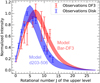 |
Fig. 8 Normalized intensities Ĩij of CH+ rovibrational transitions v = 1 → 0, J → J + 1 following chemical-pumping while considering the observed distribution of H2 and temperature. The red (resp. blue) line corresponds to the intensities of CH+ considering the temperature and H2 population densities in the Bar (resp. in d203-506). The shaded areas indicate the range between the upper and lower limits as determined in Sect. 5.2.1. Red (resp. blue) crosses correspond to the normalized intensities of CH+ transitions observed in the Bar (resp. disk). |
6 Discussion
6.1 Diagnostics on chemistry and physical conditions
In the previous section, we used the relative line intensities to support that the vibrational bands of CH+ detected in the Orion Bar and d203-506 are excited by chemical pumping. When a line is excited by chemical pumping, its absolute intensity carries crucial information about the local conditions.
6.1.1 Formation rate of CH+ by C+ + H2*
Following the formalism of Zannese et al. (2024) used for OH chemical-pumping excitation, we can estimate a formation rate of CH+ from the intensities measured in the observations and the model of chemical-pumping. Here, we assume that, in both environments, the impact of radiative pumping and inelastic collisions is negligible. Furthermore, the rovibrational excited lines are found to be optically thin. Hence, the intensities Iij are simply proportional to R, the formation rate of CH+ as described in Eq. (8). Thus, the formation rate can be calculated as follows:
 (10)
(10)
From the observed intensities and the population distribution of CH+, we derive R = (2.0–6.0) × 1010 cm−2 s−1 in the Bar and R = (1.5–4.5) × 1011 cm−2 s−1 in d203-506. The formation rate of CH+ is about 7 times higher in the disk than in the Bar. A brief summary of the important results of our study is presented in Table 1.
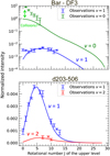 |
Fig. 9 Normalized intensities Ĩij of CH+ of v = 0 → 0, J → J–1 (green), v =1 → 0, J → J + 1 (blue), and v = 2 → 1, J → J + 1 (red) following chemical-pumping while considering the observed population densities of H2 and temperature in the Bar and d203-506. Emissions from v = 1 and v = 2 levels are observed with NIRSpec. Emission from v = 0 levels are observed with Herschel/PACS and Herschel/HIFI, and we considered that the emission comes from a 2′′ wide filament (Joblin et al. 2018). |
6.1.2 Gas density
Zannese et al. (2024) showed that chemical pumping models of O + H2 can be used to estimate the local density. Here, we follow this formalism because of the similarity of processes (O + H2 vs C+ + H2). Hence, the formation rate, integrated over the line of sight, of CH+ via C++H2 corresponds to
 (11)
(11)
where nC+ and nH2 are the number densities of ionized carbon and molecular hydrogen and k(T, xj(H2)) is the total formation rate ([cm3 s−1]):
 (12)
(12)
Assuming a homogeneous medium, the local density can be estimated from the inferred value of R from Eq. (11) as
 (13)
(13)
where N(H2) is the column density of H2, x(C+) is the ionized carbon abundance, and nH is the total number density of hydrogen nuclei.
In both environments, the ionized carbon abundance can be taken around x(C+) ≃ 1.4 × 10⁻⁴ (Sofia et al. 1997). In d203-506, we measure a column density of warm H2 of N(H2) = 8.7 × 1019 cm−2 and a temperature of T ≃ 850 K (Berné et al. 2023). We derive a total rate coefficient of k = (2.5–2.6) × 10−12 cm3 s−1 from Eq. (12), and using the H2 excitation diagram and the state-specific rates of Zanchet et al. (2013); Faure et al. (2017); Neufeld et al. (2021). Using the estimate of R = (1.5–4.5) × 1011 cm−2 s−1 from the CH+ near-IR lines, we derive nH = (0.6–2.0) × 107 cm−3. Interestingly, the intensity derived by this diagnostic gives a similar value as the very similar diagnostic made by Zannese et al. (2024) with chemical pumping for the OH molecule via O + H2. This is also in agreement with the estimation made from a different approach by Berné et al. (2024) using H2 lines and the Meudon PDR Code (Le Petit et al. 2006).
Similarly, in the Bar, the column density of warm H2 is N(H2) = 1.6 × 1021 cm−2 and the temperature is T ≃ 570 K from the rotational lines (Van De Putte et al. 2024, Zannese & Sidhu in prep). From the estimation of temperature and excitation of H2, we derive the coefficient rate k = (2.1–2.2) × 10−13 cm3 s−1. Using the estimate of R = (2.0–6.0) × 1010 cm−1 s−1 from the CH+ near-IR lines, we derive nH = (0.6–1.5) × 106 cm−3. This value leads to a thermal pressure for the dissociation front to be around Pgas ≃ 3–7 × 10⁸ K cm−3. One should know that the uncertainties of extrapolated rates are difficult to estimate. However, we assumed that they are negligible considering other sources of uncertainties, which we discuss below.
This density estimate is higher than what is found from the H2 emission (Pgas ∼ 5 × 10⁷−2 × 10⁸ K cm−3, Joblin et al. 2018; Van De Putte et al. 2024, Meshaka et al. in prep, Zannese & Sidhu in prep). Whether the thermal pressure is constant all over the dissociation front (e.g., Bron et al. 2018) is difficult to affirm as the spatial resolution is not sufficient to actually probe the variation of density and temperature across the DF. Here, we assume a single-layer model which does not consider any variation in physical conditions. We have shown previously that the CH+ lines are more sensitive to the density than the highly excited H2 (see Fig. 4). They may be more influenced by the higher density part of the front and thus trace a higher thermal pressure than what is derived from the overall emission of H2 (rotational and rovibrational). Moreover, to increase the S/N of the CH+ line detection, we derived the intensities from a large aperture. This means that the population densities of H2 are also averaged. By averaging the population densities of H2, we probably underestimate the proportion of H2 in highly excited states in comparison to the lowest excited states at the position where CH+ peaks. Underestimating these levels leads to overestimating the gas density. Indeed, as they have more internal energy, they are more reactive and will enhance the formation of CH+ in excited states. We can use models to estimate how the averaging of H2 population densities can impact the density. We use the best-fit model from the Meudon PDR Code (Le Petit et al. 2006) reproducing H2 emission at Pgas = 5 × 10⁷ K cm−3 (Meshaka et al., in prep.). We calculated H2 population densities, H2 column density and temperature at the peak of the line H2 1–0 S(1) and the peak of the line H2 0–0 S(1). The value of k × N(H2) averaged around the peak of H2 1–0 S(1) is about 5 times larger than around the peak of H2 0–0 S(1). Interestingly, this factor is similar even in a higher thermal pressure model (Pgas=5 × 10⁸ K cm−3). Thus, using the equation Eq. (13), the derived density can be overestimated by as much as a factor 5 according to models. The use of self-consistent models, such as the Meudon PDR Code, including CH+ chemical pumping, is necessary to provide more accurate predictions considering the steep variation of physical parameters. It will also be useful to validate our zero-dimensional models by comparing them to PDR models, taking into account the depth of the cloud. However, this further modeling is beyond the scope of this paper.
6.2 Alternative excitation processes
To ensure that the observed lines are only excited by chemical pumping, we need to verify that other excitation processes cannot explain the observed spectrum. Moreover, the first two lines of CH+, v = 1 P(1) and P(2), detected in the Bar cannot be explained by the chemical pumping model (see Fig. 9).
6.2.1 IR pumping
IR pumping can be an efficient process to excite the first vibrational state since it takes the absorption of only one near-infrared photon to bring CH+ to a v = 1, J state. If IR pumping is relevant to excite the observed levels, then the brightness temperature of the infrared radiation TIR around 3.5–4.5 μm has to be similar to the vibrational excitation temperature Tvib,
 (14)
(14)
where Jλ is the intensity of the infrared radiation field at the wavelength λ (in W m−2 Hz−1 sr−1). If the field is isotropic, Jλ = Iλ where Iλ is the specific intensity observed in the line of sight, corrected for extinction at the wavelength λ. Around 3.5–4.5 μm, Iλ ∼ 100 MJy sr−1 in DF3 and Iλ ∼ 300 MJy sr−1 in d203-506. If the infrared radiation field is not isotropic, it is possible its intensity at the H/H2 transition is higher than what we observe in the line of sight. Another estimation of the infrared radiation field at the dissociation front can be made if we consider that it is mainly emitted by nanograins in the atomic zone. The specific intensity at the dissociation front is then half the intensity of the radiation field in the atomic zone as it is only coming from ahead. In the atomic zone, Iλ ∼ 250 MJy sr−1. Thus, both estimations of the infrared radiation field at DF3 are very similar. We then derive TIR ∼ 150–190 K in DF3 and d203-506. As a result of different rotational temperatures in the v = 0 and v = 1 levels detected in DF3, the vibrational temperature, calculated from Eq. (4), varies from Tvib ∼ 290 K to Tvib ∼ 650 K. These temperatures are much higher than that of the near-infrared radiation.
In addition, as radiative pumping only changes J by Δ J = ± 1, it is expected that the v = 1 rotational distribution would mirror the v = 0 rotational distribution. Figure 5 shows that the rotational distributions are very different in the v = 0 and v = 1, at least for J > 2. Thus, we conclude that IR pumping is unlikely to account for the excitation of the high-J rotational levels in v = 1 but also for the first two, which cannot be explained by chemical pumping.
In d203-506, we cannot measure the vibrational temperature between v = 0 and v = 1 because there is no data available for the detection of purely rotational lines of CH+. However, the vibrational temperature between v = 1 and v = 2, being around Tvib ∼ 1300 K, is also incompatible with IR pumping.
Finally, in these environments, collisions are expected to be more important the radiative pumping. Indeed, radiative pumping would dominate over collisions with atomic hydrogen to excite a level i if
 (15)
(15)
However, for all J levels of CH+,  in DF3 and 10−6 in d203-506. This means that radiative pumping does not dominate over collisions with hydrogen. In the next section, we discuss collisions against chemical pumping.
6.2.2 Collisions
It is difficult to evaluate accurately the contribution of collisions in the excitation of the v = 1 state since the inelastic collisional rates between v = 1 and v = 0 remain poorly known. Only collisional rates with electrons for the rovibrational excitation have been calculated (Jiang et al. 2019; Forer et al. 2023). For other collisional partners, only the collisional rates for the rotational levels have been calculated, for atomic hydrogen (Faure et al. 2017) and helium (Hammami et al. 2009).
Using the collisional rates with electrons from Forer et al. (2023), we find that the collisions with electrons play a negligible role in the excitation of the v = 1 state compared to chemical pumping in both environments. Indeed, comparing the total excitation rate of the v = 1 band by collisions and by chemical pumping, collisions with electrons are dominant when
 (16)
(16)
where kchem,v=1 is the formation rate of C+ + H2 leading to CH+(v = 1) and kcoll,v=1 is the total collisional excitation rate connecting the v = 0 and the v = 1 state. At the H/H2 transition, C+ is the main positive charge carrier so x(C+) ≃ x(e−). Thus Eq. (16) can be rewritten as
 (17)
(17)
Forer et al. (2023) finds kcoll, v = 1(1000 K) ≃ 2 × 10⁻⁹ cm3 s−1 and kcoll, v=1(600 K) ≃ 2 × 10⁻¹⁰ cm3 s−1. Quantitatively, we find that collisions become dominant for x(CH+)/x(H2) ≳ 6 × 10⁻⁵ in d203-506 and in DF3. According to PDR models representative of d203-506 (see Extended Data Fig. 7 from Berné et al. 2023), x(CH+) ∼ 3 × 10⁻⁷ giving x(CH+)/x(H2) ∼ 6 × 10⁻⁷. According to PDR models around Pgas = 5 × 10⁷−108 K cm−3 and G0 = 104, x(CH+) ∼ 10−7 in DF3, thus x(CH+)/x(H2) ∼ 2 × 10⁻⁷. In conclusion, collisions with electrons are not dominant in both environments as they would contribute to 1% at most to the excitation of the v = 1 state compared with chemical pumping.
However, it is possible that in those environments, collisions with atomic hydrogen are more important than collisions with electrons. Collisions with atomic hydrogen to excite the v = 1 level are the dominant process when
 (18)
(18)
At the H/H2 transition, x(H) ≃ x(H2). Thus Eq. (18) can be rewritten as
 (19)
(19)
This means that chemical pumping tends to be favored if the abundance of the considered species is low compared to the reactants that form it. The collisional rates with H for the rovibrational levels of CH+ are not available. However, using the extrapolation made from Faure et al. (2017) by Neufeld et al. (2021), we can estimate the collisional excitation rate of the v = 1 state at T = 1000 K considering the CH+ rotational population of the v = 0 level at LTE, to be kcoll, v=1(1000 K) ≃ 4 × 10⁻¹² cm3 s−1 and at T = 600 K to be kcoll, v=1(600 K) ≃ 3 × 10⁻¹³ cm3 s−1. Thus, collisions become dominant for x(CH+)/x(C+) > 5 × 10⁻² in DF3 and x(CH+)/x(C+) > 3 × 10⁻² in d203-506. Considering x(C+) ≃ 1.4 × 10⁻⁴, we have x(CH+)/x(C+) ∼ 10−3 in DF3 and x(CH+)/x(C+) ∼ 3 × 10⁻³ in d203-506. Therefore, we find that collisions with atomic hydrogen would not dominate over chemical pumping in the excitation of the v = 1 state. However, we observe that collisions with H are more efficient than collisions with electrons and can contribute up to 10% of the excitation of the v = 1 band compared with chemical pumping.
Our finding that collision contributes little to the excitation of the v = 1 state can be seen at odd with the discrepancy between the chemical pumping model and the low-J v = 1 lines seen in the DF1. In fact, up to now, our discussion ignores the rotational distribution of CH+, which should be considered when collisional excitation rates are not negligible compared to the chemical pumping rate. Collisional excitation of the v = 1 is dominated by collisional transitions starting from the low-J levels of the v = 0 state since those levels are much more populated than higher-J levels (see excitation diagram Fig. 5). As a consequence, the collisions populate preferentially the low-J levels of the v = 1 due to a combination of the propensity rules (Δ J= ± 1, ± 2) and the minimization of the energy gap. In other words, we naturally expect collisions to affect the low-J v = 1 lines. In contrast, chemical pumping directly produces CH+ within the v = 1 state in higher J-levels. This likely explains why our chemical-pumping model fails only for the lowest J lines within the v = 1 state by underestimating their emission. It is likely that in d203-506, CH+ rotational levels within v = 0 are more evenly populated due to the higher gas temperature and density. This would make the population of the v = 1 levels by collision more distributed in the different rotational levels and thus less visible than in DF3. In any case, the excellent agreement between the chemical-pumping model and the observations of d203-506 remains the most compelling evidence that collisional excitation is negligible in this source for v = 1 and v = 2.
We also stress that CH+ is highly reactive and can be destroyed by reaction with H2 and H atoms very rapidly. This high reactivity could hamper the inelastic collision efficiency as an excitation process. In any case, to properly conclude if collisions can explain the v = 1, J = 0, 1 levels detected in DF3, we need the calculations of the collisional rates of CH+ vibrational bands.
6.3 Discussion on gas-phase chemistry
6.3.1 Role of carbon grain destruction
Throughout this study, we provide evidence that CH+ is formed and excited by C+ + H2. Indeed, the spatial correlation between H2 and CH+ and the comparison between observed intensities and chemical pumping models shows that both in the Bar and d203-506, the observations can be explained by the gas phase formation route.
This conclusion is more difficult to make for  . At the moment, there is no available theoretical or experimental data on the state-resolved reaction
  .
.  is a 4 atoms system, which complicates the modeling of such processes due to the increased number of exit channels. However, several aspects of the observations are striking.
  is detected at the same position as H2 and CH+. Moreover, in the Bar, its excitation temperature is higher than the gas temperature and higher than the excitation temperature estimated in d203-506, similarly to CH+. Moreover, if CH+ is formed in the gas phase,
  must be a dominant outcome by the chain reaction of Eq. (2) because the reactions of CH+ + H2 and
  are exothermic for all H2(v, J) contrary to C+ + H2.
If  is not formed in the gas phase, could it be produced by photodestruction of PAHs? Previous studies have shown the importance of this mechanism in small hydrocarbons abundance in the Horsehead Nebula. Indeed, in this region, state-of-the-art chemical models, which do not take PAH photodestruction process into account, fail to reproduce the abundances of observed hydrocarbons at the PDR edge (Pety et al. 2005; Guzmán et al. 2015). This has been further supported by Alata et al. (2014, 2015) who showed experimentally that small hydrocarbons can be produced by the photolysis of hydrogenated amorphous carbon when exposed to UV photons. When implementing the experimentally determined reaction parameters in a time-dependent astrophysical model with parameters typical of the Horsehead Nebula, these authors showed that the abundance of small hydrocarbons can temporarily rise by several orders of magnitude. However, these studies do not state the possibility of producing hydrocarbons that are highly hydrogenated, such as
  . The methyl radical would have to come from a methyl side group of a PAH, and it is more likely that the methyl group would first lose an hydrogen atom while possibly isomerizing into a tropylium-like structure (Geballe et al. 1989; Joblin et al. 1996; Zhen et al. 2016). Studies on PAH photodestruction mainly reveal the formation of hydrocarbons with small carbon chains containing at least two carbons, and no ionization is expected from neutral fragmentation. To this date, there is still no detection of the nonpolar species CH4 and C2 H2 in the Orion Bar, which are expected to be the main products of the photodestruction of PAHs or amorphous carbon grains. In addition, Cuadrado et al. (2015) observed a variety of small hydrocarbons in this region with the IRAM 30 m telescope and has been able to explain their abundances only with gas phase chemistry (see also Goicoechea et al. 2025). Finally, it is also hard to conceive that
  could be produced with such an excitation temperature in the Bar through the photodestruction of small grains.
All these results are in favor of the hypothesis that  is formed and chemically pumped in the gas phase (see Eq. (2)) under the conditions explored here in Orion. State-to-state rate coefficients of the chemical pumping of
  through the reaction
  are essential to properly conclude this matter.
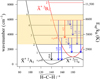 |
Fig. 10 Energy level diagram of the bending levels in the two lowest electronic states of |


6.3.2 Searching for CH2+
In the gas-phase route, we thus detected two crucial intermediates: CH+ and  . Assuming this route predominantly forms
  (see Eq. (2)), the question arises: what happens to
  , the intermediate step between CH+ and
  ?
?  possesses three vibrational modes, the symmetric stretching mode (v1), the bending mode (v2), and the asymmetric stretching mode (v3) and their corresponding fundamentals in its electronic ground state are located around ∼ 3.47 μm (2883.0 cm−1) (Kraemer et al. 1994), ∼ 10.05 μm (995.5 cm−1) (Kraemer et al. 1994), and ∼ 3.19 μm (3131.4 cm−1) (Rösslein et al. 1992), respectively. Following the logic behind the detection of CH+ and
  , one would expect the detection of
  based on the emission from v2 around 10 μm supposed to be the brightest. The existing experimental data in the literature do not allow us to model a high-resolution gas phase emission spectrum for this band due to the lack of spectroscopic information about the rotational constants of the v2 = 1 vibrational state. Only the rotational constants of the ground state are well characterized (Rösslein et al. 1992; Willitsch & Merkt 2003; Gottfried & Oka 2004). The fundamental band of this mode has been reported theoretically (Osmann et al. 1997) and experimentally (Bunker et al. 2001). These results constrain the search for this emission feature from
  between 9 and 11 μm, a region where there are no remaining unassigned observed transitions in the JWST spectra of DF3 and d203-506 (see Fig. 11). The search of
  signatures in the v1 and v3 band in the NIR was also unsuccessful. In addition, no unidentified lines in the ISO and Herschel/PACS spectrum can be assigned to
  rotational emission. This raises the intriguing issue as to why CH+ and
  can be detected by their emission fingerprints while
  cannot, despite astrochemical models forecasting comparable abundances for
  and
and  (see Extended Data Fig. 7 of Berné et al. 2023). Mazo-Sevillano et al. (2024) predicts that
  is slightly less abundant than
  which could explain its non detection, if it is not chemically pumped, in the Bar but not in d203-506.
A better understanding of  spectroscopic properties is required to assess how compatible this non-detection is with current predictions by astrochemical models. The initial step to answer this question involves describing the strong vibronic couplings known to be present in
  bending modes and giving rise to a rich manifold of potential transitions (see Fig. 10) and assessing the population distribution of
  in the energy level structure during the process of its formation from the addition of H2 to CH+. In the absence of specific information on the state distribution of
  in the Orion Bar, the formation of
  in its first electronic excited state (Ã+) has also to be considered.
  could present vibrational emission from its least energetic vibrational mode (v2 = 1 → v2 = 0 in Ã+), which should be located around ∼ 4 μm (2500 cm−1). Alternatively, it could relax to its ground electronic state (
 ) by vibronic emission. If one estimates that only the first vibrational levels of the Ã+ state are populated based on CH+ and
  temperatures in the Orion Bar (estimated to lie between about 700 and 1500 K), the strongest emission transitions will be toward the excited vibrational levels of
  . Emission features of
  could therefore originate from the v2 = 0 and v2 = 1 of the Ã+ electronic state toward the v2 bending levels of the
  electronic state (Wang et al. 2013; Bunker et al. 2007). Expected ranges for such transitions are reported in Fig 10. Moreover, Bunker et al. (2007) finds that the strongest of these bands are in the near-infrared range around 0.9 μm. Typical vibronic emission has a larger probability than vibrational emission, which could explain the elusiveness of
  as its spectroscopic signatures could be spread and contribute in another spectral region of the JWST spectra.
The emission spectrum of  in the hot environment of the Orion Bar and d203-506 could actually be located in the NIR region, especially if
  is produced in vibrational states higher than v2 = 1 in the Ã+ electronic state. Some lines are still unidentified in the JWST NIR spectrum (Peeters et al. 2024), but the identification to
  has not been made. The precise calculation of
  spectroscopy is necessary to compare the strength of the different possible transitions (v1, v2, v3) and conclude on its non-detection. Moreover, further investigation of
  formation pathways and degree of excitation are required to estimate the population of the à state in order to evaluate the importance of rovibronic transitions. However, due to the complexity of the calculations, this is referred to a future study.
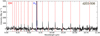 |
Fig. 11 Continuum and OFF position subtracted spectrum of the disk d203-506 between 9 and 11 μm with the identified lines. The OH lines highlighted in red were previously presented and analyzed in Zannese et al. (2024). |
6.3.3 CH3+ as the origin of warm organic chemistry
As stated previously,  is hypothesized to be at the origin of most of the complex organic chemistry in the UV-irradiated gas. By reacting with small hydrocarbons,
  can produce long-chain hydrocarbons. A variety of hydrocarbons are indeed detected with the IRAM 30m telescope, Herschel, and ALMA in the Orion Bar (Cuadrado et al. 2015; Nagy et al. 2015; Goicoechea et al. 2025). Interestingly,
  is also one of the origins of very abundant molecules such as HCO+, which is the direct product of the reaction
 (20)
(20)
As the atomic oxygen is very abundant, this reaction is as important as the formation of HCO+ from CO+ + H2 = HCO+ + H as predicted by PDR models (see Extended Data Fig. 7 and 8 of Berné et al. 2023). Thus,  is an important source of CO as well. This is compatible with previous studies that have shown the spatial coincidence between the rotational lines of HCO+ and the rovibrational emission of H2 in the Orion Bar (Goicoechea et al. 2016; Habart et al. 2023) and recent observations with ALMA of HCO+ J = 4−3 presented in Berné et al. (2024) which follows quite well the H2 and
  emission in. Interestingly, a tentative signature of the Q-branch of HCO+ is found around 12 μm in d203-506 with MIRI-MRS (see Fig. A.1), which would be the IR counterpart of the rotational emission detected by ALMA and the third species detected by JWST in this reaction chain. The analysis of this signature is beyond the scope of this paper and referred to futur investigations. In any case, our analysis reveals the first steps of the chemical route that starts from C+ and opens new avenues to consistently analyze the emission of other species detected through their rotational or rovibrational emissions.
7 Conclusion
In this work, we have studied the rovibrational emission of CH+ and  in the Orion Bar and established constraints on their formation route and excitation. We have also explored the potential of NIR CH+ emission as a diagnostic for the study of interstellar PDRs and disks. The main conclusions of this study can be summarized as follows:
The
 rovibrational emission and excited H2 emission originate from the same regions. They trace a thin layer of the H0/H2 transition where the emission from FUV-pumped H2 levels peak, too;
Both CH+ and
 have a higher excitation temperature in the Bar than the gas temperature (Tex (Bar) ∼ 1500 K > Tgas(Bar) ∼ 570 K). In addition, they have a higher excitation temperature in the Bar than in d203-506, even if the gas temperature in the disk is higher, Tex(d 203-506) ∼ 850 K ∼ Tgas(d203-506) ∼ 850 K;
Study of the observed column densities of CH+ and
 in their rovibrational states showed that the observed emission traces only a small fraction of the total abundance of these molecules, less than 0.1% in the Bar. Indeed, for both molecules, the column density derived from the rovibrational lines is around
  , while the total expected column densities are around
  ∼ 1014−1015 cm−2;
The excitation of CH+ and probably
 can be explained by chemical formation pumping with excited H2. This is in favor of a formation route in the gas phase following
  ;
;In-depth study of the chemical formation pumping mechanism showed that in regions where the temperature and density are high (such as d203-506), the excitation of CH+ is mostly driven by H2 rotational levels, which are populated by collisions. In contrast, in regions where the temperature is not as high and the gas is less dense but highly irradiated (such as the Bar), the excitation is mostly driven by FUV-pumped levels of H2;
Chemical formation pumping models can be used to determine the formation rate of CH+ in the Orion Bar and d203-506;
The emission strength of CH+ and
 depends strongly on the local density. As the excitation of CH+ follows a nonthermal process, a simple diagnostic gives access to the gas density at the H/H2 transition. This diagnostic provides an estimate of nH ≃ 107 cm−3 in d203-506 and nH ≃ 106 cm−3 in the Bar. The latter might be overestimated due to the use of large apertures to derive line intensities;
Attempts to detect
 , the intermediate between CH+ and
  , were unsuccessful. However, the complexity of
  spectroscopy could explain its non-detection, even if it has similar abundances to CH+ and
  .
.
 . However, they are essential to understanding the formation and excitation process of this molecule.
Acknowledgement
We would like to thank I. Schneider, for our fruitful discussion on collisions between CH+ and e−, which helped us discuss this matter. This work is based [in part] on observations made with the NASA/ESA/CSA James Webb Space Telescope. The data were obtained from the Mikulski Archive for Space Telescopes at the Space Telescope Science Institute, which is operated by the Association of Universities for Research in Astronomy, Inc., under NASA contract NAS 5-03127 for JWST. These observations are associated with program ERS1288. This work was partially supported by the Programme National “Physique et Chimie du Milieu Interstellaire” (PCMI) of CNRS/INSU with INC/INP. This work was supported by CNES with funds focused on JWST. J.R.G. thanks the Spanish MCINN for funding support under grant PID2023-146667NB-I00. E.P. and J.C. acknowledge support from the University of Western Ontario, the Institute for Earth and Space Exploration, the Canadian Space Agency (CSA, 22JWGO1-16), and the Natural Sciences and Engineering Research Council of Canada. This article is based upon work from COST Action CA21126 – Carbon molecular nanostructures in space (NanoSpace), supported by COST (European Cooperation in Science and Technology).
Appendix A Tentative detection of HCO+ in MIRI-MRS
A tentative detection in MIRI-MRS of HCO+ is presented in Fig. A.1. The comparison to simulated spectra at T = 100 K and T = 200 K shows rather cold emission of HCO+. The exact excitation of HCO+ needs further investigation. The excitation temperature is lower than the gas temperature questions, pointing toward subthermal excitation of the rotational levels, which might be explained by IR pumping. However, the proper analysis of this signature is referred to a future study.
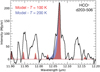 |
Fig. A.1 Tentative detection of HCO+ in the disk d203-506 with MIRI-MRS. Two models at T = 100 K (in red) and T = 200 K (in blue) using spectroscopic data from Davies et al. (1984); Foster et al. (1984) are superposed to the observations. |
Appendix B Importance of non-LTE distribution of H2 in chemical pumping
Figure B.1 shows that taking into account the observed non-LTE distribution of H2 in the CH+ chemical models is highly important for DF3. In d203-506, the modeled intensities for an H2 LTE distribution and the observed distribution is very similar. This highlights the importance of thermalized levels of H2 in the excitation of CH+ in the disk. Thus, we find that in environments with high temperatures, pure rotational levels of H2 are sufficient to excite CH+ in the v = 1 level. When the temperature is lower, the FUV-pumped levels of H2 have higher importance in the excitation.
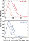 |
Fig. B.1 Comparison of modeled chemical pumping intensities of CH+ using LTE distribution of H2 at the gas temperature and the observed distribution in the Orion Bar. (Top) Modeled intensities for DF3. (Bottom) Modeled intensities for d203-506. Taking into account FUV-pumped levels of H2 is highly important in DF3 compared to d203-506. |
Appendix C Dependence of chemical pumping rates of CH+(v = 1) on H2 levels (v′, J′)
Figure C.1 shows the dependence of chemical pumping rates of CH+(v = 1) on different H2 levels and on gas temperature. We find that H2 levels with high excitation are able to populate higher-J levels of CH+. When E(H2) > E(CH+) + Δ E, the rate coefficients depend neither on the temperature nor on the levels energy of CH+ and H2 anymore.
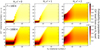 |
Fig. C.1 Probability to populate one rotational level of CH+ (v = 1) from one level of H2. Only the chemical pumping rates from the v′ = 1, J′ = 0, 1 and v′ = 2, J′ = 0 levels of H2 are available (Zanchet et al. 2013; Faure et al. 2017). The other rates come from the extrapolation made in Neufeld et al. (2021). Two regimes can be observed. The first and flat one (J′ < 10 for v′ = 0) is when E(H2) < E(CH+) + Δ E. The second one, cone-like (J′ > 10 for v′ = 0), is when E(H2) > E(CH+) + Δ E and the chemical pumping rate depends neither on the temperature nor on the levels energy of CH+ and H2 anymore. |
Appendix D CH+ line intensities in the Bar and d203-506
Table D.1 presents the CH+ line intensities detected in DF3 not and corrected for extinction and in d203-506.
Intensities of the CH+ lines detected in DF3 and in d203-506. The uncertainties are only the fitting error. The impact of calibration effects is not taken into account, and the associated uncertainties can be as high as 20%.
Appendix E Observed spectra of CH+ and  in the Bar and in d203-506
E.1 CH+
Figure E.1 displays the observed spectra of CH+ in DF3 and d203-506 with fitted LTE models.
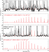 |
Fig. E.1 (a): (Top) CH+ continuum subtracted spectra in DF3 (see Fig. 1); (bottom) LTE model of CH+ at T = 1500 K and Nvib(CH+) = 7.6 × 109 cm−2. The column density of the fit is lower due to extinction in the line of sight. (b): (Top) CH+ continuum subtracted spectra in d203-506 (see Fig. 1). (Bottom) LTE model of CH+ at T = 850 K and Nvib(CH+) = 3 × 1011 cm−2. |
E.2 
Fig. E.2 displays the observed spectra of  in DF3 and d203-506 with fitted LTE models.
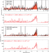 |
Fig. E.2 (a): (Top) |


Appendix F Post-processing of the JWST spectra
F.1 CH+
Fig. F.1 displays the post-processing of the NIRSpec observed spectra to better visualize CH+ lines in DF3 and d203-506.
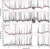 |
Fig. F.1 Processing of the NIRSpec spectrum. (a) DF3: (Top panel) Spectrum observed with NIRSpec. The red line is the estimated continuum. (Bottom panel) Continuum subtracted spectrum. (b) Disk: (Top panel) Spectrum observed with NIRSpec. The red line is the estimated continuum. (Bottom panel) Continuum subtracted spectrum. Red vertical lines are CH+ v = 1–0 transitions, and blue lines are CH+ v = 2–1 transitions. Other line identifications can be found in Peeters et al. (2024). |
F.2 
Fig. F.2 displays the post-processing of the MIRI-MRS observed spectra to better visualize the  feature in DF3 and d203-506.
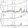 |
Fig. F.2 Processing of the MIRI-MRS spectrum. (a) DF3: (Top panel) Spectrum observed with MIRI-MRS. The red line is the estimated continuum. (Bottom panel) Continuum subtracted spectrum. (b) Disk: (Top panel) Spectrum observed with MIRI-MRS. The red line is the estimated continuum. (Bottom panel) Continuum subtracted spectrum. All the observed lines are from |

F.3 HCO+
Fig. F.3 displays the post-processing of the MIRI-MRS observed spectra to better visualize HCO+ feature in d203-506.
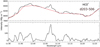 |
Fig. F.3 Processing of the MIRI spectrum. (Top panel) Spectrum observed with MIRI. The red line is the estimated continuum. (Bottom panel) Continuum subtracted spectrum. |
References
- Agúndez, M., Goicoechea, J. R., Cernicharo, J., Faure, A., & Roueff, E. 2010, ApJ, 713, 662 [Google Scholar]
- Alata, I., Cruz-Diaz, G. A., Muñoz Caro, G. M., & Dartois, E. 2014, A&A, 569, A119 [NASA ADS] [CrossRef] [EDP Sciences] [Google Scholar]
- Alata, I., Jallat, A., Gavilan, L., et al. 2015, A&A, 584, A123 [NASA ADS] [CrossRef] [EDP Sciences] [Google Scholar]
- Asvany, O., Thorwirth, S., Redlich, B., & Schlemmer, S. 2018, J. Mol. Spectrosc., 347, 1 [NASA ADS] [CrossRef] [Google Scholar]
- Berné, O., Habart, É., Peeters, E., et al. 2022, PASP, 134, 054301 [CrossRef] [Google Scholar]
- Berné, O., Martin-Drumel, M.-A., Schroetter, I., et al. 2023, Nature, 621, 56 [CrossRef] [Google Scholar]
- Berné, O., Habart, E., Peeters, E., et al. 2024, Science, 383, 988 [Google Scholar]
- Black, J. H. 1998, Faraday Discuss., 109, 257 [NASA ADS] [CrossRef] [Google Scholar]
- Bron, E., Agúndez, M., Goicoechea, J. R., & Cernicharo, J. 2018, arXiv e-prints [arXiv:1801.01547] [Google Scholar]
- Bruderer, S., Benz, A. O., van Dishoeck, E. F., et al. 2010, A&A, 521, L44 [NASA ADS] [CrossRef] [EDP Sciences] [Google Scholar]
- Bunker, P., Chan, M., Kraemer, W., & Jensen, P. 2001, Chem. Phys. Lett., 341, 358 [NASA ADS] [CrossRef] [Google Scholar]
- Bunker, P. R., Kraemer, W. P., Yurchenko, S. N., et al. 2007, Mol. Phys., 105, 1369 [Google Scholar]
- Cernicharo, J., Liu, X. W., González-Alfonso, E., et al. 1997, ApJ, 483, L65 [NASA ADS] [CrossRef] [Google Scholar]
- Changala, P. B., Neufeld, D. A., & Godard, B. 2021, ApJ, 917, 16 [NASA ADS] [CrossRef] [Google Scholar]
- Changala, P. B., Chen, N. L., Le, H. L., et al. 2023, A&A, 680, A19 [NASA ADS] [CrossRef] [EDP Sciences] [Google Scholar]
- Chown, R., Sidhu, Ameek, Peeters, Els, et al. 2024, A&A, 685, A75 [NASA ADS] [CrossRef] [EDP Sciences] [Google Scholar]
- Coudert, L., Gans, B., Holzmeier, F., et al. 2018, J. Chem. Phys., 149, 224304 [NASA ADS] [CrossRef] [Google Scholar]
- Cuadrado, S., Goicoechea, J. R., Pilleri, P., et al. 2015, A&A, 579, C1 [NASA ADS] [CrossRef] [EDP Sciences] [Google Scholar]
- Cunha de Miranda, B. K., Alcaraz, C., Elhanine, M., et al. 2010, J. Phys. Chem. A, 114, 4818 [CrossRef] [Google Scholar]
- Davies, P. B., Hamilton, P. A., & Rothwell, W. J. 1984, J. Chem. Phys., 81, 1598 [NASA ADS] [CrossRef] [Google Scholar]
- Douglas, A. E., & Herzberg, G. 1941, ApJ, 94, 381 [NASA ADS] [CrossRef] [Google Scholar]
- Falgarone, E., Godard, B., Cernicharo, J., et al. 2010, A&A, 521, L15 [NASA ADS] [CrossRef] [EDP Sciences] [Google Scholar]
- Faure, A., Halvick, P., Stoecklin, T., et al. 2017, MNRAS, 469, 612 [NASA ADS] [CrossRef] [Google Scholar]
- Foster, S. C., McKellar, A. R. W., & Sears, T. J. 1984, J. Chem. Phys., 81, 578 [NASA ADS] [CrossRef] [Google Scholar]
- Forer, J., Hvizdoš, D., Ayouz, M., Greene, C., & Kokoouline, V. 2023, MNRAS, 527, 5238 [NASA ADS] [CrossRef] [Google Scholar]
- Geballe, T. R., Tielens, A. G. G. M., Allamandola, L. J., Moorhouse, A., & Brand, P. W. J. L. 1989, ApJ, 341, 278 [NASA ADS] [CrossRef] [Google Scholar]
- Gerin, M., Neufeld, D. A., & Goicoechea, J. R. 2016, ARA&A, 54, 181 [NASA ADS] [CrossRef] [Google Scholar]
- Godard, B., & Cernicharo, J. 2013, A&A, 550, A8 [NASA ADS] [CrossRef] [EDP Sciences] [Google Scholar]
- Goicoechea, J. R., & Roncero, O. 2022, A&A, 664, A190 [NASA ADS] [CrossRef] [EDP Sciences] [Google Scholar]
- Goicoechea, J. R., Pety, J., Cuadrado, S., et al. 2016, Nature, 537, 207 [Google Scholar]
- Goicoechea, J. R., Santa-Maria, M. G., Bron, E., et al. 2019, A&A, 622, A91 [NASA ADS] [CrossRef] [EDP Sciences] [Google Scholar]
- Goicoechea, J. R., Le Bourlot, J., Black, J. H., et al. 2024, A&A, 689, L4 [NASA ADS] [CrossRef] [EDP Sciences] [Google Scholar]
- Goicoechea, J. R., Pety, J., Cuadrado, S., et al. 2025, A&A, 696, A100 [NASA ADS] [CrossRef] [EDP Sciences] [Google Scholar]
- Gordon, K. D., Clayton, G. C., Decleir, M., et al. 2023, ApJ, 950, 86 [CrossRef] [Google Scholar]
- Gottfried, J. L., & Oka, T. 2004, J. Chem. Phys., 121, 11527 [NASA ADS] [CrossRef] [Google Scholar]
- Guzmán, V. V., Pety, J., Goicoechea, J. R., et al. 2015, ApJ, 800, L33 [CrossRef] [Google Scholar]
- Habart, E., Dartois, E., Abergel, A., et al. 2010, A&A, 518, L116 [CrossRef] [EDP Sciences] [Google Scholar]
- Habart, E., Le Gal, R., Alvarez, C., et al. 2023, A&A, 673, A149 [NASA ADS] [CrossRef] [EDP Sciences] [Google Scholar]
- Habart, E., Peeters, Els, Berné, Olivier, et al. 2024, A&A, 685, A73 [NASA ADS] [CrossRef] [EDP Sciences] [Google Scholar]
- Habing, H. J. 1968, Bull. Astron. Inst. Netherlands, 19, 421 [Google Scholar]
- Hammami, K., Owono Owono, L. C., & Stäuber, P. 2009, A&A, 507, 1083 [NASA ADS] [CrossRef] [EDP Sciences] [Google Scholar]
- Haworth, T. J., Reiter, M., O’Dell, C. R., et al. 2023, MNRAS, 525, 4129 [NASA ADS] [CrossRef] [Google Scholar]
- Henning, T., Kamp, I., Samland, M., et al. 2024, PASP, 136, 054302 [NASA ADS] [CrossRef] [Google Scholar]
- Herbst, E. 2021, Front. Astron. Space Sci., 8, 207 [NASA ADS] [CrossRef] [Google Scholar]
- Hierl, P. M., Morris, R. A., & Viggiano, A. A. 1997, J. Chem. Phys., 106, 10145 [Google Scholar]
- Hollenbach, D. J., & Tielens, A. G. G. M. 1997, ARA&A, 35, 179 [NASA ADS] [CrossRef] [Google Scholar]
- Inoguchi, M., Hosokawa, T., Mineshige, S., & Kim, J.-G. 2020, MNRAS, 497, 5061 [NASA ADS] [CrossRef] [Google Scholar]
- Jensen, P., Brumm, M., Kraemer, W., & Bunker, P. 1995, J. Mol. Spectrosc., 172, 194 [NASA ADS] [CrossRef] [Google Scholar]
- Jiang, X., Yuen, C. H., Cortona, P., Ayouz, M., & Kokoouline, V. 2019, Phys. Rev. A, 100, 062711 [NASA ADS] [CrossRef] [Google Scholar]
- Joblin, C., Tielens, A. G. G. M., Allamandola, L. J., & Geballe, T. R. 1996, ApJ, 458, 610 [NASA ADS] [CrossRef] [Google Scholar]
- Joblin, C., Bron, E., Pinto, C., et al. 2018, A&A, 615, A129 [NASA ADS] [CrossRef] [EDP Sciences] [Google Scholar]
- Jones, M. E., Barlow, S., Ellison, G., & Ferguson, E. 1986, Chem. Phys. Lett., 130, 218 [NASA ADS] [CrossRef] [Google Scholar]
- Kaplan, K. F., Dinerstein, H. L., Oh, H., et al. 2017, ApJ, 838, 152 [CrossRef] [Google Scholar]
- Kaplan, K. F., Dinerstein, H. L., Kim, H., & Jaffe, D. T. 2021, ApJ, 919, 27 [NASA ADS] [CrossRef] [Google Scholar]
- Keceli, M., Shiozaki, T., Yagi, K., & Hirata, S. 2009, Mol. Phys., 107, 1283 [CrossRef] [Google Scholar]
- Kraemer, W., & Špirko, V. 1991, J. Mol. Spectrosc., 149, 235 [NASA ADS] [CrossRef] [Google Scholar]
- Kraemer, W., Jensen, P., & Bunker, P. 1994, Can. J. Phys., 72, 871 [NASA ADS] [CrossRef] [Google Scholar]
- Le Petit, F., Nehmé, C., Le Bourlot, J., & Roueff, E. 2006, ApJ, 164, 506 [Google Scholar]
- Mazo-Sevillano, P. d., Aguado, A., Goicoechea, J. R., & Roncero, O. 2024, J. Chem. Phys., 160, 184307 [NASA ADS] [CrossRef] [Google Scholar]
- Menten, K. M., Reid, M. J., Forbrich, J., & Brunthaler, A. 2007, A&A, 474, 515 [NASA ADS] [CrossRef] [EDP Sciences] [Google Scholar]
- Nagy, Z., Van der Tak, F. F. S., Ossenkopf, V., et al. 2013, A&A, 550, A96 [NASA ADS] [CrossRef] [EDP Sciences] [Google Scholar]
- Nagy, Z., Ossenkopf, V., Van der Tak, F. F. S., et al. 2015, A&A, 578, A124 [NASA ADS] [CrossRef] [EDP Sciences] [Google Scholar]
- Naylor, D. A., Dartois, E., Habart, E., et al. 2010, A&A, 518, L117 [NASA ADS] [CrossRef] [EDP Sciences] [Google Scholar]
- Neufeld, D. A., Godard, B., Bryan Changala, P., et al. 2021, ApJ, 917, 15 [NASA ADS] [CrossRef] [Google Scholar]
- Osmann, G., Bunker, P. R., Jensen, P., & Kraemer, W. P. 1997, Chem. Phys., 225, 33 [NASA ADS] [CrossRef] [Google Scholar]
- Parikka, A., Habart, E., Bernard-Salas, J., et al. 2017, A&A, 599, A20 [NASA ADS] [CrossRef] [EDP Sciences] [Google Scholar]
- Peeters, E., Habart, E., Berné, O., et al. 2024, A&A, 685, A74 [NASA ADS] [CrossRef] [EDP Sciences] [Google Scholar]
- Pety, J., Teyssier, D., Fossé, D., et al. 2005, A&A, 435, 885 [NASA ADS] [CrossRef] [EDP Sciences] [Google Scholar]
- Rangwala, N., Maloney, P. R., Glenn, J., et al. 2014, ApJ, 788, 147 [Google Scholar]
- Rösslein, M., Gabrys, C., Jagod, M.-F., & Oka, T. 1992, J. Mol. Spectrosc., 153, 738 [CrossRef] [Google Scholar]
- Smith, D. 1992, Chem. Rev., 92, 1473 [Google Scholar]
- Sofia, U. J., Cardelli, J. A., Guerin, K. P., & Meyer, D. M. 1997, ApJ, 482, L105 [NASA ADS] [CrossRef] [Google Scholar]
- Spinoglio, L., Pereira-Santaella, M., Busquet, G., et al. 2012, ApJ, 758, 108 [Google Scholar]
- Stecher, T. P., & Williams, D. A. 1972, ApJ, 177, L141 [NASA ADS] [CrossRef] [Google Scholar]
- Sternberg, A., & Dalgarno, A. 1995, ApJS, 99, 565 [NASA ADS] [CrossRef] [Google Scholar]
- Tabone, B., van Hemert, M. C., van Dishoeck, E. F., & Black, J. H. 2021, A&A, 650, A192 [NASA ADS] [CrossRef] [EDP Sciences] [Google Scholar]
- Thi, W. F., Ménard, F., Meeus, G., et al. 2011, A&A, 530, L2 [NASA ADS] [CrossRef] [EDP Sciences] [Google Scholar]
- Van De Putte, D., Meshaka, R., Trahin, B., et al. 2024, A&A, 687, A86 [NASA ADS] [CrossRef] [EDP Sciences] [Google Scholar]
- van der Tak, F. F. S., Nagy, Z., Ossenkopf, V., et al. 2013, A&A, 560, A95 [NASA ADS] [CrossRef] [EDP Sciences] [Google Scholar]
- Veselinova, A., Agúndez, M., Goicoechea, J. R., et al. 2021, A&A, 648, A76 [NASA ADS] [CrossRef] [EDP Sciences] [Google Scholar]
- Wang, H., Neese, C. F., Morong, C. P., Kleshcheva, M., & Oka, T. 2013, J. Phys. Chem. A, 117, 9908 [NASA ADS] [CrossRef] [Google Scholar]
- Wesson, R., Cernicharo, J., Barlow, M. J., et al. 2010, A&A, 518, L144 [NASA ADS] [CrossRef] [EDP Sciences] [Google Scholar]
- Willitsch, S., & Merkt, F. 2003, J. Chem. Phys., 118, 2235 [NASA ADS] [CrossRef] [Google Scholar]
- Wolfire, M. G., Vallini, L., & Chevance, M. 2022, ARA&A, 60, 247 [NASA ADS] [CrossRef] [Google Scholar]
- Zanchet, A., Godard, B., Bulut, N., et al. 2013, ApJ, 766, 80 [NASA ADS] [CrossRef] [Google Scholar]
- Zannese, M., Tabone, B., Habart, E., et al. 2023, A&A, 671, A41 [NASA ADS] [CrossRef] [EDP Sciences] [Google Scholar]
- Zannese, M., Tabone, B., Habart, E., et al. 2024, Nat. Astron., 8, 577 [Google Scholar]
- Zhen, J., Castellanos, P., Linnartz, H., & Tielens, A. G. G. M. 2016, Mol. Astrophys., 5, 1 [NASA ADS] [CrossRef] [Google Scholar]
https://pdrs4all.org/, DOI: 10.17909/pg4c-1737
Available on MAST PDRs4All website: https://doi.org/10.17909/wqwy-p406
All Tables
Intensities of the CH+ lines detected in DF3 and in d203-506. The uncertainties are only the fitting error. The impact of calibration effects is not taken into account, and the associated uncertainties can be as high as 20%.
All Figures
|
Fig. 1 JWST NIRCam composite image of the Orion Bar located in the Orion molecular cloud (Habart et al. 2024). Red is the 3.35 μm emission (F335M NIRCam filter), blue is the emission of Paα (F187N filter subtracted by F182M filter) and green is the emission of the H2 0–0 S(9) line at 4.70 μm (F470N filter subtracted by F480M filter). The |
| In the text | |
|
Fig. 2 H2 0–0 S(9) continuum subtracted map at 4.69 μm (Zannese & Sidhu in prep). The green boxes are the aperture used to extract the spectra. (Left) CH+ v = 1–0 P(5) line at 3.86 μm. (Right) |
| In the text | |
|
Fig. 3 Normalized integrated intensity profiles of the CH+ v = 1–0 P(5) line, |
| In the text | |
|
Fig. 4 Integrated intensity ratio of CH+ v = 1–0 P(5) over H2 0–0 S(9) (top) and peak intensity ratio of |
| In the text | |
|
Fig. 5 Excitation diagram and level population of CH+ and H2 in d203-506 and in the Bar. (Left) Excitation diagram of CH+ (a) in the Bar and (c) in d203-506. (Right) Level population of H2 normalized to the total column density (see Table 1) (b) in the Bar and (d) in d203-506. The difference in H2 population distribution can explain the difference in the excitation diagram of CH+. |
| In the text | |
|
Fig. 6 Local thermodynamic equilibrium models of the Q branch of |
| In the text | |
|
Fig. 7 Line ratios of |
| In the text | |
|
Fig. 8 Normalized intensities Ĩij of CH+ rovibrational transitions v = 1 → 0, J → J + 1 following chemical-pumping while considering the observed distribution of H2 and temperature. The red (resp. blue) line corresponds to the intensities of CH+ considering the temperature and H2 population densities in the Bar (resp. in d203-506). The shaded areas indicate the range between the upper and lower limits as determined in Sect. 5.2.1. Red (resp. blue) crosses correspond to the normalized intensities of CH+ transitions observed in the Bar (resp. disk). |
| In the text | |
|
Fig. 9 Normalized intensities Ĩij of CH+ of v = 0 → 0, J → J–1 (green), v =1 → 0, J → J + 1 (blue), and v = 2 → 1, J → J + 1 (red) following chemical-pumping while considering the observed population densities of H2 and temperature in the Bar and d203-506. Emissions from v = 1 and v = 2 levels are observed with NIRSpec. Emission from v = 0 levels are observed with Herschel/PACS and Herschel/HIFI, and we considered that the emission comes from a 2′′ wide filament (Joblin et al. 2018). |
| In the text | |
|
Fig. 10 Energy level diagram of the bending levels in the two lowest electronic states of |
| In the text | |
|
Fig. 11 Continuum and OFF position subtracted spectrum of the disk d203-506 between 9 and 11 μm with the identified lines. The OH lines highlighted in red were previously presented and analyzed in Zannese et al. (2024). |
| In the text | |
|
Fig. A.1 Tentative detection of HCO+ in the disk d203-506 with MIRI-MRS. Two models at T = 100 K (in red) and T = 200 K (in blue) using spectroscopic data from Davies et al. (1984); Foster et al. (1984) are superposed to the observations. |
| In the text | |
|
Fig. B.1 Comparison of modeled chemical pumping intensities of CH+ using LTE distribution of H2 at the gas temperature and the observed distribution in the Orion Bar. (Top) Modeled intensities for DF3. (Bottom) Modeled intensities for d203-506. Taking into account FUV-pumped levels of H2 is highly important in DF3 compared to d203-506. |
| In the text | |
|
Fig. C.1 Probability to populate one rotational level of CH+ (v = 1) from one level of H2. Only the chemical pumping rates from the v′ = 1, J′ = 0, 1 and v′ = 2, J′ = 0 levels of H2 are available (Zanchet et al. 2013; Faure et al. 2017). The other rates come from the extrapolation made in Neufeld et al. (2021). Two regimes can be observed. The first and flat one (J′ < 10 for v′ = 0) is when E(H2) < E(CH+) + Δ E. The second one, cone-like (J′ > 10 for v′ = 0), is when E(H2) > E(CH+) + Δ E and the chemical pumping rate depends neither on the temperature nor on the levels energy of CH+ and H2 anymore. |
| In the text | |
|
Fig. E.1 (a): (Top) CH+ continuum subtracted spectra in DF3 (see Fig. 1); (bottom) LTE model of CH+ at T = 1500 K and Nvib(CH+) = 7.6 × 109 cm−2. The column density of the fit is lower due to extinction in the line of sight. (b): (Top) CH+ continuum subtracted spectra in d203-506 (see Fig. 1). (Bottom) LTE model of CH+ at T = 850 K and Nvib(CH+) = 3 × 1011 cm−2. |
| In the text | |
|
Fig. E.2 (a): (Top) |
| In the text | |
|
Fig. F.1 Processing of the NIRSpec spectrum. (a) DF3: (Top panel) Spectrum observed with NIRSpec. The red line is the estimated continuum. (Bottom panel) Continuum subtracted spectrum. (b) Disk: (Top panel) Spectrum observed with NIRSpec. The red line is the estimated continuum. (Bottom panel) Continuum subtracted spectrum. Red vertical lines are CH+ v = 1–0 transitions, and blue lines are CH+ v = 2–1 transitions. Other line identifications can be found in Peeters et al. (2024). |
| In the text | |
|
Fig. F.2 Processing of the MIRI-MRS spectrum. (a) DF3: (Top panel) Spectrum observed with MIRI-MRS. The red line is the estimated continuum. (Bottom panel) Continuum subtracted spectrum. (b) Disk: (Top panel) Spectrum observed with MIRI-MRS. The red line is the estimated continuum. (Bottom panel) Continuum subtracted spectrum. All the observed lines are from |
| In the text | |
|
Fig. F.3 Processing of the MIRI spectrum. (Top panel) Spectrum observed with MIRI. The red line is the estimated continuum. (Bottom panel) Continuum subtracted spectrum. |
| In the text | |
Current usage metrics show cumulative count of Article Views (full-text article views including HTML views, PDF and ePub downloads, according to the available data) and Abstracts Views on Vision4Press platform.
Data correspond to usage on the plateform after 2015. The current usage metrics is available 48-96 hours after online publication and is updated daily on week days.
Initial download of the metrics may take a while.