| Issue |
A&A
Volume 699, July 2025
|
|
|---|---|---|
| Article Number | L13 | |
| Number of page(s) | 9 | |
| Section | Letters to the Editor | |
| DOI | https://doi.org/10.1051/0004-6361/202555841 | |
| Published online | 23 July 2025 | |
Letter to the Editor
PDRs4All
XV. CH radical and H molecular ion in the irradiated protoplanetary disk d203-506
1
Institut de Recherche en Astrophysique et Planétologie, Université Toulouse III – Paul Sabatier, CNRS, CNES, 9 Av. du colonel Roche, 31028 Toulouse Cedex 04, France
2
Instituto de Física Fundamental (CSIC), Calle Serrano 121-123, 28006 Madrid, Spain
3
Department of Space, Earth, and Environment, Chalmers University of Technology, Onsala Space Observatory, 43992 Onsala, Sweden
4
Dipartimento di Fisica, Università degli Studi di Milano, Via Celoria 16, 20133 Milano, Italy
5
I. Physikalisches Institut, Universität zu Köln, Zülpicher Str.77, D-50937 Köln, Germany
6
NASA Ames Research Center, MS 245-6, Moffett Field, CA 94035-1000, USA
7
HFML-FELIX, Toernooiveld 7, 6525ED Nijmegen, The Netherlands
8
Institute for Molecules and Materials, Radboud University, Heyendaalseweg 135, 6525AJ Nijmegen, The Netherlands
9
Department of Physics & Astronomy, The University of Western Ontario, London, ON N6A 3K7, Canada
10
Institute for Earth and Space Exploration, The University of Western Ontario, London, ON N6A 3K7, Canada
11
Carl Sagan Center, Search for ExtraTerrestrial Intelligence Institute, Mountain View, CA 94043, USA
12
Institut des Sciences Moléculaires d’Orsay, CNRS, Université Paris-Saclay, 91405 Orsay, France
13
Centro de Astrobiología (CAB), CSIC-INTA, Ctra. de Ajalvir, km 4, Torrejón de Ardoz, 28850 Madrid, Spain
14
Laboratoire de Physique de l’École normale supérieure, ENS, Université PSL, CNRS, Sorbonne Université, Université Paris Cité, 75005 Paris, France
15
Observatoire de Paris, Université PSL, Sorbonne Université, LERMA, CNRS UMR 8112, 75014 Paris, France
16
Department of Astronomy, Graduate School of Science, The University of Tokyo, Tokyo 113-0033, Japan
17
LUX, UMR 8262, Observatoire de Paris, PSL Research University, CNRS, Sorbonne Universités, 92190 Meudon, France
18
Astronomy Department, University of Maryland, College Park, MD 20742, USA
19
Leiden Observatory, Leiden University, P.O. Box 9513 2300 RA Leiden, The Netherlands
20
Institut d’Astrophysique Spatiale, Université Paris-Saclay, Centre National de la Recherche Scientifique, 91405 Orsay, France
⋆ Corresponding author: ilane.schroetter@gmail.com
Received:
6
June
2025
Accepted:
3
July
2025
Most protoplanetary disks experience a phase in which they are subjected to strong ultraviolet radiation from nearby massive stars. This UV radiation can substantially alter their chemistry by producing numerous radicals and molecular ions. In this Letter we present a detailed analysis of the JWST-NIRSpec spectrum of the d203-506 obtained as part of the PDRs4All Early Release Science program. Using state-of-the-art spectroscopic data, we searched for species using a multi-molecule fitting tool, PAHTATMOL, which we developed for this purpose. Based on this analysis, we report the clear detection of ro-vibrational emission of the CH radical and the likely detection of the H3+ molecular ion, with estimated abundances of a few times 10−7 and approximately 10−8, respectively. The presence of CH is predicted by gas-phase models and is well explained by hydrocarbon photochemistry. Interstellar H3+ is usually formed through reactions of H2 with H3+ originating from cosmic ray ionization of H2. However, recent theoretical studies suggest that H3+ also forms through far-UV (FUV)-driven chemistry in strongly irradiated (G0 > 103), dense (nH > 106 cm−3) gas. The latter is favored as an explanation for the presence of hot H3+ (Tex ≳ 1000 K) in the outer disk layers of d203-506, coinciding with the emission of FUV-pumped H2 and other photodissociation region (PDR) species, such as CH+, CH3+, and OH. Our detection of infrared emission from vibrationally excited H3+ and CH raises questions about their excitation mechanisms and underscores that FUV radiation can have a profound impact on the chemistry of planet-forming disks. They also demonstrate the power of JWST to push the limit of the detection of elusive species in protoplanetary disks.
Key words: protoplanetary disks / ISM: molecules / ISM: individual objects: d203-506
© The Authors 2025
 Open Access article, published by EDP Sciences, under the terms of the Creative Commons Attribution License (https://creativecommons.org/licenses/by/4.0), which permits unrestricted use, distribution, and reproduction in any medium, provided the original work is properly cited.
This article is published in open access under the Subscribe to Open model. Subscribe to A&A to support open access publication.
1. Introduction
Ultraviolet (UV) radiation from massive stars is ubiquitous in galaxies and plays a fundamental role in the physics and the chemistry of star and planet formation (e.g., Wolfire et al. 2022). JWST spectroscopic observations of protoplanetary disks irradiated by UV radiation from massive stars have revealed that this energy input drives a chemistry dominated by abundant ions and radicals. A key signature of this photochemistry is the methyl cation CH discovered in the highly irradiated (G0 = 2 × 10⁴) protoplanetary disk d203-506 in Orion (Berné et al. 2023; Changala et al. 2023). Other tracers of these processes include the detection of rotationally hot OH (Zannese et al. 2024), the presence of the reactive ion CH+ (Berné et al. 2024; Zannese et al. 2025), and the infrared fluorescent emission from electronically excited C I (Goicoechea et al. 2024). These species reside in the upper disk layers exposed to UV radiation, while most neutral species survive in the dense inner disk regions (e.g., Schroetter et al. 2025). These findings demonstrate that JWST is an unprecedented spectroscopic tool for detecting and characterizing small ions and radicals triggered by UV-driven chemistry. This capability is relevant to a wide range of astrophysical environments, from the starburst galaxies to the atmospheres of forming protoplanets in stellar clusters. Maximizing the potential of JWST requires tools that rely on state-of-the-art spectroscopic data to identify and characterize the excitation properties of the numerous species present in the infrared. In this Letter, we present PAHTATMOL, a tool dedicated to this task, and applied to NIRSpec spectra of the irradiated protoplanetary disk d203-506. This tool supports the detection of two new species in a protoplanetary disk: CH and H
 . We present the observations of d203-506 in Sect. 2 and the fitting process of its NIRSpec spectrum and the results in Sect. 3. We describe and discuss the origin and properties of the two species in Sect. 4, and present our conclusions in Sect. 5.
2. JWST spectroscopic observations of d203-506
d203-506 is situated in the line of sight toward the Orion Bar (Bally et al. 2000), at about 0.25 pc from the massive Trapezium stars that are at a distance of ∼390 pc (Apellániz et al. 2022), inside the Orion Nebula. d203-506 is about 100 au in radius, and has an estimated mass of ∼ 10MJup as well as a central star estimated mass of M⋆ = 0.2 ± 0.1 M⊙ (Berné et al. 2024). The central star is obscured by this nearly edge-on disk (Bally et al. 2000). d203-506 was observed as part of the JWST ERS program PDRs4All (Berné et al. 2022) with NIRSpec-IFU (Böker et al. 2022). The data reduction is presented in Peeters et al. (2024). In order to obtain a high-quality spectrum of d203-506, we extracted a spectrum from the NIRSpec cube using an aperture of 0.1″ (corresponding to 39 au at 390 pc) centered on the position of the bright spot (RA = 5h35′20.314″, Dec = −5°25′05.47″) on the northwestern tip of the disk facing the illuminating star, θ1 Ori C. The resulting spectrum is presented in Figs. 1 and A.1. As we are interested in simple molecular ions and radicals in this study, we only focus on the f290 filter, spanning from 2.87 to 5.2 μm, which is where many fundamental stretching bands are present.
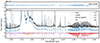 |
Fig. 1. Bottom panel: PAHTATMOL shifted fit result (blue curve) on the NIRSpec f290lp filter spectrum of d203-506 (black curve). The different colors at the bottom of the panel show the inverted individual molecular spectra, and a dotted magenta line shows the atomic and H2 emission lines. Upper panel: Model residual (observed spectrum minus the model). |
3. Fitting of the spectrum
3.1. Fitting procedure
In Appendix A we present the PAHTATMOL tool, which allows a global molecular model to be fit to an observed JWST spectrum of an irradiated disk. Briefly, this model includes broad individual Gaussians to reproduce the emission from polycyclic aromatic hydrocarbons (PAHs), blackbodies to reproduce the stellar and disk dust continuum emission, and the ro-vibrational emission from multiple molecular species. Here we include emission from 19 species, which are listed in Table A.1. This list includes simple species previously observed in disks such as CO, OH, HCO+, and CH+, but also a number of other species that have not yet been detected in disks (e.g., CH, H ), and species not detected in space at all (e.g., C2H
 ). For all species we used state-of-the-art public spectroscopic data and computed their global emission assuming local thermodynamical equilibrium (LTE), meaning that the ro-vibrational levels follow a Boltzmann distribution at a single excitation temperature (Tex)1. PAHTATMOL provides a first-order simulation, allowing a simultaneous fit over the full JWST wavelength range that includes all potential ro-vibrational lines (blended or not) of the species that might be present. Thus, PAHTATMOL provides LTE column densities (N) and excitation temperatures Tex, assuming single-slab radiative transfer. In protoplanetary disks, gas densities are typically high enough that, for many molecular species, the rotational temperature (Trot) of the low-lying rotational levels in the ground vibrational state tends to approximate the gas temperature, with Trot ≲ Tgas. For instance, the infrared H2 rotational emission observed in the irradiated layers of d203-506, with Trot ≃ 1000 K (Berné et al. 2024), provides a good measure of the aperture-averaged gas temperature.
3.2. Fit results
Figure 1 shows the resulting best-fit model using PAHTATMOL over the 2.87 to 5.2 μm wavelength range (corresponding to NIRSpec f290lp filter). In this range, we are able to reproduce the vast majority (≥90%) of the lines present in the data2. In particular, we report the detections of CO, CH, CH+, OH, and H . We note that the estimated excitation temperatures, hereafter T, provided by the PAHTATMOL fit are to be taken as indicators rather than precise values, and are given with an error of ∼ ± 300 K. For both CO and H
 , the best-fit temperatures are a combination of T = 1000 K and 2000 K. This implies that two components are needed to fit the data, likely tracing the molecule’s presence along a temperature gradient. For all species, the derived temperatures are high (≥1000 K), indicating their presence in UV-irradiated hot gas and-or excitation by formation or radiative pumping (e.g., Zannese et al. 2025).
4. New detections in a protoplanetary disk
In addition to the previously detected species CO, OH, and CH+, we used PAHTATMOL to report, according to our detection threshold definition (see Appendix A.2), the first detections of CH (see Fig. 2) and H (see Figs. 4 and B.1) in a protoplanetary disk. In the following we discuss the implications of these detections.
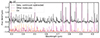 |
Fig. 2. Near-infrared CH rovibrational emission in d203-506. The continuum-subtracted observations are shown in black, and the CH model–offset for clarity–is shown in orange. The dotted magenta lines indicate model spectra for additional species. |
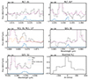 |
Fig. 4. H |


4.1. Methylidyne radical: CH
The methylidyne radical has been detected in the interstellar medium and has been used as a powerful tracer of molecular hydrogen and of the initial steps of hydrocarbon chemistry (e.g., Gerin et al. 2010). We detect the CH ro-vibrational emission lines around 3.3 μm in the same wavelength range of the 3.3–3.4 μm PAH emission bands (C–H stretching). The detected CH emission lines correspond to both the R branch (< 3.62 μm) and the P branch (> 3.68 μm). For CH, we find a temperature T ≃ 2000 K and a column density of 4.5 × 1014 cm−2. Using the H2 column density derived by Berné et al. (2024) and assuming N(H) = N(H2) in the disk PDR, we infer a CH abundance of a few 10−7 with respect to H nuclei.
The bottom left panel of Fig. 3 shows the spatial distribution of the CH 3.426 μm emission line. This emission is slightly less extended than that of vibrationally excited H2 (e.g., as traced by the v = 1 − 0 S(1) line emission) and implies that CH arises from deeper layers of the disk PDR. Our photochemical models (see Appendix C) show that, as for CH+ and CH , CH is a natural product of simple hydrocarbon photochemistry (see the chemical sketch in Fig. 11 of Goicoechea et al. 2025) triggered by the presence of C+ ions, C atoms, elevated temperatures, and the enhanced reactivity of excited H2 (Berné et al. 2024). Compared to CH+ and CH
 , the model suggests that most of the CH column density originates from slightly deeper layers within the PDR (see Fig. C.1), where CH is formed through the dissociative recombination of CH
 and through reactions of atomic carbon with vibrationally excited H2. Figure 1 of Berné et al. (2023) shows that the IR CH+ and CH
 emission peak toward the outermost irradiated disks layers (the bright spot), whereas CH peaks deeper inside the disk PDR (Fig. 3). Our photochemical model predicts N(CH) ≲ 1014 cm−2, which is a factor of ≲ 5 lower than the estimated LTE column density. This might suggest that other chemical routes contribute to CH formation–such as its indirect production through PAH or carbonaceous grain photodestruction. Alternatively, reactions of electronically excited far-UV (FUV)-pumped C atoms with H2 may play a role (e.g., González-Lezana 2007; Goicoechea et al. 2024), or, more likely, radiative pumping contributes to CH excitation (see Appendix of Berné et al. 2023, for CH
 ) as CH exhibits strong electronic transitions in the visible and FUV (e.g., Oka et al. 2013), which can be excited by external starlight.
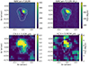 |
Fig. 3. IR JWST images of d203-506. Top left: NIRCam F182M (broad filter centered at 1.82 μm). Top right: NIRCam F212N (H2 1-0 S(1) emission). Bottom left: NIRSpec CH emission map, continuum subtracted. Bottom right: NIRSpec Q(1,0) H |

4.2. Trihydrogen cation: H
The trihydrogen cation, H , is the electronically simplest stable polyatomic molecule. Figure 4 shows the likely detection of several H
 emission lines from the ν2 = 1 → 0 band, including the R(1,0), Q(1,0), Q(5,G)3, R(7,0)l, and R(7,6)u lines. The reported lines are weak and lie near the detection threshold, but the stacked spectrum clearly shows an emission feature (see details in Appendix B). Table B.1 summarizes the transition properties. Other expected H
 lines are blended with emission lines from other abundant species, leaving the presence of H
 emission in d203-506 open to interpretation. In Fig. B.1, we show the complete best-fit H
 emission model for each ν2 = 1 → 0 branch (R, Q, and P) and compare it with the observed minus source-model spectrum. Pereira-Santaella et al. (2024) recently reported the detection of H
 (in emission and absorption) in the interstellar medium of galaxies using JWST-NIRSpec. The higher-energy H
 lines reported in d203-506 (Fig. 4) are not observed in the galaxies, suggesting that the excitation conditions in the disk–specifically the gas temperature and density–are higher. Interestingly, some of these excited lines, for instance the Q(5,0) line, are detected in the ionosphere of Jupiter (Oka & Geballe 1990). Our detection would represent the first identification of H
 in a protoplanetary disk.
The H emission in d203-506 peaks near the bright spot (see bottom right panel of Fig. 3), which also coincides with the peak of near-IR H2v = 1–0 S(1) emission. This region corresponds to gas that is strongly illuminated by FUV radiation. The H
 emission also overlaps with the emission peak of highly excited rotational lines of OH, a clear indication of water vapor photodissociation (Zannese et al. 2024). We find T ≥ 1000 K and a column density of 1.1×1013 cm−2, thus an abundance of a few 10−8, using the same circular surface area as for CH. Given the very large radiative transition probabilities of the H
 ro-vibrational emission lines (on the order of ∼100 s−1), these lines cannot be thermalized (Tvib ≠ Tgas) by inelastic collisions at the densities of ∼107 cm−3 expected in the disk PDR (e.g., Berné et al. 2024). It is therefore important to distinguish between the best-fitting LTE temperature, which approximately reflects the rotational excitation, and the vibrational excitation temperature. The presence of vibrationally excited H
 emission in protoplanetary disks raises important questions regarding the mechanisms driving its formation and the excitation of these levels–whether through chemical pumping, radiative pumping, or both. In a companion paper, Goicoechea et al. (2025) find that H
 can efficiently form in strongly irradiated (G0 > 103) dense gas through chemical routes involving a hot water vapor reservoir, triggered by UV radiation, and largely independent of the cosmic-ray ionization rate. For d203-506, they predict a H
 column density of ≲1013 cm−2 in the disk PDR, in good agreement with the value estimated here.
5. Conclusion and outlook
We claim the detection of two new molecules in a protoplanetary disk: the methylidyne radical (CH) and the trihydrogen cation (H ). The detection of CH, which shows a slightly different spatial emission distribution compared to that of CH+ and CH
 (Berné et al. 2023), is consistent with the expectations of PDR hydrocarbon chemistry driven by the high gas temperature and enhanced reactivity of excited H2, which efficiently converts C+ ions and C atoms into simple hydrocarbons. The presence of infrared H
 emission in the disk’s PDR component, if confirmed, would suggest that chemical formation routes unrelated to cosmic-ray ionization contribute to its formation.
The detection of hot vibrationally excited CH and H underscores the need to explore the non-LTE excitation mechanisms of these species, which will be the subject of future papers. All in all, we expect these two new molecules to be present in the IR spectra of other strongly irradiated protoplanetary disks.
In many cases, however, the infrared emission arises from non-LTE excitation (Tex ≠ Tgas)–for instance, driven by radiative or chemical formation pumping–which requires more sophisticated models that explicitly solve the statistical equilibrium equations, incorporating the IR-to-UV radiation field and both chemical formation and destructionprocesses (e.g., Zannese et al. 2024, 2025 for OH, CH , and CH+).
The spikes in the residual (difference) spectrum (see the upper panel of Fig. 1) arise from strong emission lines, caused by inaccuracies in the simplified modeling of the excitation conditions.
We model this reaction from Dean et al. (1991) by adopting v-state-dependent rate constants where the energy Ev, J of each H2(v) ro-vibrational state is subtracted from the reaction endoergicity ΔE (when ΔE > Ev, J). That is, kv, J(T) ∝ exp( − [ΔE − Ev, J]/kBT).
Acknowledgments
We thank the referees for her/his comments and suggestions, which helped improve the clarity of the manuscript. This work is based [in part] on observations made with the NASA/ESA/CSA James Webb Space Telescope. The data were obtained from the Mikulski Archive for Space Telescopes at the Space Telescope Science Institute, which is operated by the Association of Universities for Research in Astronomy, Inc., under NASA contract NAS 5-03127 for JWST. These observations are associated with programs #1288. IS, OB are funded by the Centre National d’Etudes Spatiales (CNES) through the APR program. This research received funding from the program ANR-22-EXOR-0001 Origins of the Institut National des Sciences de l’Univers, CNRS. This project is co-funded by the European Union (ERC, SUL4LIFE, grant agreement No101096293). AF also thanks project PID2022-137980NB-I00 funded by the Spanish Ministry of Science and Innovation/State Agency of Research MCIN/AEI/10.13039/501100011033 and by “ERDF A way of making Europe”. C.B. acknowledges support from the Internal Scientist Funding Model (ISFM) Laboratory Astrophysics Directed Work Package at NASA Ames (22-A22ISFM-0009) and is grateful for an appointment at NASA Ames Research Center through the San José State University Research Foundation (80NSSC22M0107).
References
- Altman, R. S., Crofton, M. W., & Oka, T. 1984a, J. Chem. Phys., 81, 4255 [Google Scholar]
- Altman, R. S., Crofton, M. W., & Oka, T. 1984b, J. Chem. Phys., 80, 3911 [Google Scholar]
- Apellániz, J. M., Barbá, R., Aranda, R. F., et al. 2022, A&A, 657, A131 [NASA ADS] [CrossRef] [EDP Sciences] [Google Scholar]
- Asvany, O., Giesen, T., Redlich, B., & Schlemmer, S. 2005, Phys. Rev. Lett., 94, 073001 [Google Scholar]
- Bally, J., O’Dell, C., & McCaughrean, M. J. 2000, AJ, 119, 2919 [NASA ADS] [CrossRef] [Google Scholar]
- Bast, M., Böing, J., Salomon, T., et al. 2023, J. Mol. Spectr., 398, 111840 [Google Scholar]
- Bernath, P. F. 2020, J. Quant. Spectr. Rad. Transf., 240, 106687 [NASA ADS] [CrossRef] [Google Scholar]
- Berné, O., Habart, É., Peeters, E., et al. 2022, PASP, 134, 054301 [CrossRef] [Google Scholar]
- Berné, O., Martin-Drumel, M. A., Schroetter, I., et al. 2023, Nature, 621, 56 [Google Scholar]
- Berné, O., Habart, E., Peeters, E., et al. 2024, Sci, 383, 988 [Google Scholar]
- Böker, T., Arribas, S., Lützgendorf, N., et al. 2022, A&A, 661, A82 [NASA ADS] [CrossRef] [EDP Sciences] [Google Scholar]
- Bowesman, C. A., Mizus, I. I., Zobov, N. F., et al. 2023, MNRAS, 519, 6333 [Google Scholar]
- Brooke, J. S., Bernath, P. F., Western, C. M., et al. 2016, J. Quant. Spectr. Rad. Transf., 168, 142 [NASA ADS] [CrossRef] [Google Scholar]
- Changala, P. B., Chen, N. L., Le, H. L., et al. 2023, A&A, 680, A19 [NASA ADS] [CrossRef] [EDP Sciences] [Google Scholar]
- Crofton, M. W., Altman, R. S., Haese, N. N., & Oka, T. 1989, J. Chem. Phys., 91, 5882 [Google Scholar]
- Dean, A. J., Davidson, D., & Hanson, R. 1991, J. Phys. Chem., 95, 183 [Google Scholar]
- Doménech, J. L., Jusko, P., Schlemmer, S., & Asvany, O. 2018, ApJ, 857, 61 [Google Scholar]
- Foschino, S., Berné, O., & Joblin, C. 2019, A&A, 632, A84 [EDP Sciences] [Google Scholar]
- Gerin, M., De Luca, M., Goicoechea, J., et al. 2010, A&A, 521, L16 [NASA ADS] [CrossRef] [EDP Sciences] [Google Scholar]
- Goicoechea, J. R., Le Bourlot, J., Black, J. H., et al. 2024, A&A, 689, L4 [NASA ADS] [CrossRef] [EDP Sciences] [Google Scholar]
- Goicoechea, J., Pety, J., Cuadrado, S., et al. 2025, A&A, 696, A100 [NASA ADS] [CrossRef] [EDP Sciences] [Google Scholar]
- Goicoechea, J. R., Roncero, O., Roueff, E., et al. 2025, A&A, submitted, [arXiv:2506.05189] [Google Scholar]
- González-Lezana, T. 2007, Int. Rev. Phys. Chem., 26, 29 [Google Scholar]
- Gordon, I. E., Rothman, L. S., Hill, C., et al. 2017, J. Quant. Spectr. Rad. Transf., 203, 3 [Google Scholar]
- Gorman, M. N., Yurchenko, S. N., & Tennyson, J. 2019, MNRAS, 490, 1652 [Google Scholar]
- Gruebele, M., Polak, M., & Saykally, R. J. 1987, J. Chem. Phys., 87, 3347 [Google Scholar]
- Haworth, T. J., Reiter, M., O’Dell, C. R., et al. 2023, MNRAS, 525, 4129 [NASA ADS] [CrossRef] [Google Scholar]
- Hodges, J. N., & Bernath, P. F. 2017, ApJ, 840, 81 [Google Scholar]
- Jagod, M.-F., Rösslein, M., Gabrys, C. M., et al. 1992, J. Chem. Phys., 97, 7111 [Google Scholar]
- Lattanzi, V., Walters, A., Drouin, B. J., & Pearson, J. C. 2007, ApJ, 662, 771 [NASA ADS] [CrossRef] [Google Scholar]
- Le Petit, F., Nehmé, C., Le Bourlot, J., & Roueff, E. 2006, ApJS, 164, 506 [NASA ADS] [CrossRef] [Google Scholar]
- Li, G., Gordon, I. E., Rothman, L. S., et al. 2015, ApJS, 216, 15 [NASA ADS] [CrossRef] [Google Scholar]
- Lindsay, C. M., & McCall, B. J. 2001, J. Mol. Spectr., 210, 60 [Google Scholar]
- Liu, D.-J., Haese, N. N., & Oka, T. 1985, J. Chem. Phys., 82, 5368 [Google Scholar]
- Masseron, T., Plez, B., Van Eck, S., et al. 2014, A&A, 571, A47 [NASA ADS] [CrossRef] [EDP Sciences] [Google Scholar]
- Miller, S., Tennyson, J., Geballe, T. R., & Stallard, T. 2020, Rev. Mod. Phys., 92, 035003 [NASA ADS] [CrossRef] [Google Scholar]
- Mizus, I. I., Alijah, A., Zobov, N. F., et al. 2017, MNRAS, 468, 1717 [NASA ADS] [CrossRef] [Google Scholar]
- Oka, T. 1980, Phys. Rev. Lett., 45, 531 [CrossRef] [Google Scholar]
- Oka, T., & Geballe, T. R. 1990, ApJ, 351, L53 [Google Scholar]
- Oka, T., Welty, D. E., Johnson, S., et al. 2013, ApJ, 773, 42 [NASA ADS] [CrossRef] [Google Scholar]
- Peeters, E., Habart, E., Berné, O., et al. 2024, A&A, 685, A74 [NASA ADS] [CrossRef] [EDP Sciences] [Google Scholar]
- Pereira-Santaella, M., González-Alfonso, E., García-Bernete, I., et al. 2024, A&A, 689, L12 [NASA ADS] [CrossRef] [EDP Sciences] [Google Scholar]
- Perri, A. N., & McKemmish, L. K. 2024, MNRAS, 531, 3023 [Google Scholar]
- Pilleri, P., Montillaud, J., Berné, O., & Joblin, C. 2012, A&A, 542, A69 [NASA ADS] [CrossRef] [EDP Sciences] [Google Scholar]
- Schlemmer, S., Plaar, E., Gupta, D., et al. 2024, Mol. Phys., 122, e2241567 [Google Scholar]
- Schmid, P. C., Asvany, O., Salomon, T., Thorwirth, S., & Schlemmer, S. 2022, J. Phys. Chem. A, 126, 8111 [Google Scholar]
- Schroetter, I., Berné, O., Bron, E., et al. 2025, Nat. Astron., in press, https://doi.org/10.1038/s41550-025-02596-6 [Google Scholar]
- Siller, B. M., Hodges, J. N., Perry, A. J., & McCall, B. J. 2013, J. Phys. Chem. A, 117, 10034 [Google Scholar]
- Somogyi, W., Yurchenko, S. N., & Yachmenev, A. 2021, J. Chem. Phys., 155 [Google Scholar]
- Tang, J., & Oka, T. 1999, J. Mol. Spectr., 196, 120 [Google Scholar]
- Tennyson, J., Yurchenko, S. N., Al-Refaie, A. F., et al. 2016, J. Mol. Spectr., 327, 73 [NASA ADS] [CrossRef] [Google Scholar]
- Western, C. M. 2017, J. Quant. Spectr. Rad. Transf., 186, 221 [NASA ADS] [CrossRef] [Google Scholar]
- Wolfire, M. G., Vallini, L., & Chevance, M. 2022, ARA&A, 60, 247 [NASA ADS] [CrossRef] [Google Scholar]
- Yousefi, M., Bernath, P. F., Hodges, J., & Masseron, T. 2018, J. Quant. Spectrosc. Rad. Transf., 217, 416 [Google Scholar]
- Yurchenko, S. N., Sinden, F., Lodi, L., et al. 2018, MNRAS, 473, 5324 [NASA ADS] [CrossRef] [Google Scholar]
- Zannese, M., Tabone, B., Habart, E., et al. 2024, Nat. Astron., 8, 577 [Google Scholar]
- Zannese, M., Tabone, B., Habart, E., et al. 2025, A&A, 696, A99 [NASA ADS] [CrossRef] [EDP Sciences] [Google Scholar]
Appendix A: PAHTATMOL
While atomic emission lines are quite straightforward to detect in astronomical spectra due to their temperature independent line ratios and well known line positions, the detection of molecules requires more intensive modeling, since their relative line intensities and thus emission pattern depends on the excitation temperature. A complete spectroscopic model, derived most often from laboratory spectroscopic studies, is needed to predict the emission spectra at different temperatures. Once this is known, specific molecules can be identified in an astrophysical object, and their excitation temperature and abundance can be derived from fitting the relative and absolute intensities to the observations. With the new JWST spectroscopic data allowing for fine molecular detection and even the discovery of new molecules like CH (Berné et al. 2023; Changala et al. 2023), being able to quickly find the presence of every available molecule in the observation is of great importance. We aim to provide a tool to search for the different molecules across JWST’s wavelength coverage (0.9 − 28 μm) and also derive the column densities of those detected species, if the geometry of the system is known4. This tool is called PAHTATMOL and focuses on small molecules, radicals and ions in the UV-irradiated environment but also includes atoms, neutral and ionized.
PAHTATMOL stands for Polycyclic Aromatic Hydrocarbons Toulouse Astronomical Templates with MOLecules. This tool is based on the PAHTAT tool (Pilleri et al. 2012; Foschino et al. 2019), which fits spectra using linear methods. It assumes that each PDR spectrum is a linear combination of continuum, emission lines, AIBs (Aromatic Infrared Bands) and noise. In PAHTATMOL, we include the contribution from molecules.
A.1. Computation of molecular emission spectra
In PAHTATMOL, we focus on small molecules, radicals and ions in the UV-irradiated environments. Molecules are chosen using the most probable chemical paths in such environment. The 19 molecules focusing on hydrides, ions and radicals and are the following: CH, CH+, OH, OH+, NH, HCl, CO, 13CO, H , H3O+ SH, HeH+, HCO+, SiH, HCN+, HCNH+, C3H+, C2H
 , and CH
 . To obtain an estimation of the excitation temperature of each species, we need to model their emission at different temperatures. In our case, the temperature range is from 300 to 2000 K. To fit the spectrum using a linear combination of molecular emissions we generate, for each molecule, one spectrum at each temperature over the wavelength range of 0.9 to 27 μm to match JWST NIRSpec and MIRI MRS. The PGOPHER program is used for this.
Molecules included in PAHTATmol, with references to the spectroscopic parameters used to compute the emission spectra.
PGOPHER (Western 2017) is a versatile program designed for the simulation and fitting of rotational, vibrational, and electronic spectra of molecules. It allows to generate a LTE spectrum of a molecule from either molecular constants or from provided state and transition files. The aim of using PGOPHER is to generate, for each molecule cited previously, five spectra corresponding to temperatures of 300, 500, 1000, 1500 and 2000 K, respectively. Each spectrum is generated using either states and transition files from the EXOMOL database (Tennyson et al. 2016) or from molecular constants from the literature. In PGOPHER, each spectrum is generated between 350-12000 cm−1 (0.9-28 μm) and convolved by a Gaussian with a FWHM of 0.3 cm−1, corresponding to NIRSpec resolution, and sampled with at least 100 000 points. In addition, we set the spectra intensity units to W/molecule, which will allow a column density estimate for each detected molecule. The generated spectrum is then exported and split into two parts: NIRSpec and MIRI/MRS wavelength ranges, resampled to each instrument’s spectral resolution. Finally, we add each spectrum into the PAHTATMOL library. The list of molecules and references for the adopted spectroscopic data are given in Table A.1.
A.2. Fitting a spectrum with PAHTATMOL
Given a JWST spectrum, we can now fit the spectrum the same way as PAHTAT but adding the generated molecule spectra. As in Foschino et al. (2019) we use a non negative least square algorithm to estimate each molecule contribution. We choose to use a linear combination of molecule contribution because it is faster than non linear methods. The resulting fit gives us factors needed to reproduce the data for each molecule. From these factors and the residue of the fit (data-model), we can assess if one molecule is detected based on multiple parameters.
To assess if a molecule is detected, we first select the molecules with a non null coefficient from the results. We then compute the ratio between the molecule emission positions times the fitted factor Fmol and divide by the standard deviation of the residuals at the same position across 20 spectral pixels. This gives us a signal to noise ratio (S/N). This S/N formula is given by
![$$ \begin{aligned} \mathrm{S/N} = \sqrt{\sum _n \left({F_{\rm mol} \times I_{\mathrm{peak}_n} \over {\sigma _{\mathrm{peak}_n} [\pm 10]}}\right)^2}, \end{aligned} $$](/articles/aa/full_html/2025/07/aa55841-25/aa55841-25-eq54.gif)
with peakn being the n’s peak position and Ipeakn the intensity of the n’s peak, and σpeakn[±10] the standard deviation of the spectrum to fit ranging ten spectral pixels and centered at the peak position. We define the detection threshold as S/N > 5. According to our definition, we clearly detect CH, CH+, CO, H and OH. For CH we obtained S/N = 48, for CH+ S/N = 13, for CO S/N of 40, and for both H
 and OH S/N = 8. For each detected molecules, Fmol provides an estimation of its LTE column density with N ≈ Fmol × d2/S, taking into account the surface S of the extracted spectrum aperture and the distance d to the object.
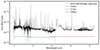 |
Fig. A.1. d203-506 NIRSpec spectrum in black. Each NIRSpec filter wavelength coverage is shown below the spectrum. |
Appendix B: Spectroscopy of H
H , with two electrons, is the electronically simplest stable polyatomic molecule. Having the symmetry of an equilateral triangle with no permanent dipole moment, it does not exhibit a rotational spectrum. Also, H
 is unstable in its singlet electronically excited state, and no sharp electronic spectrum is known (e.g., Oka et al. 2013). However, it has two vibrational modes ν1 and ν2, of which the latter is IR active. It was first detected in the laboratory by Oka (1980), with a band origin at ∼4 μm (2521.6 cm−1).
The rotational states of the ground vibrational state are characterized by two quantum numbers: the total angular momentum J and its projection onto the symmetry axis  . Since the proton is a fermion, the Pauli exclusion principle requires that all states be antisymmetric under the exchange of hydrogen nuclei. As a result, the rotational ground state
  is forbidden, making J = 1 the lowest possible state for H
 . H
. H exists in two spin isomers, distinguished by the total nuclear spin
  : ortho-H
 with
with  and the quantum number K = 3n, and para-H
 with I = 1/2 and K = 3n ± 1. For the ν2 excited state, an extra quantum number is needed for the vibrational angular momentum, l = ± 1, in addition to J and K. While the parity is given by
  , as in the ground state, the ortho and para labels depend on whether K − l is a multiple of 3. Therefore, a quantum number G ≡ |K−l| is used for convenience (for details and spectroscopic constants see Mizus et al. 2017). For the ground state, we have l = 0, G = K. The selection rules for the ν2 = 0→1 ro-vibrational transitions are ΔJ = 0 or ± 1, and ΔG = 0 (e.g., Oka et al. 2013; Miller et al. 2020). In this work we detect the following lines: R(7, 0), R(7, 6)u, R(1, 0), Q(1, 0) and Q(5, G)l (G = 0, 1, 2 and 3) (notations are from Lindsay & McCall 2001) from the ν2 band (see Fig 4). Those lines are the ones that are not blended with other emission lines (apart from R(1, 0) for which a CH emission line is partially blended with it). To increase the line sensitivity and support the detection of H
 , we looked for a line emission feature in the stacked spectra. We selected wavelength windows around the H
 lines listed in Table B.1, as well as the R(3, 3)l and Q(3, 0) lines, centered at 3.534 and 3.986 μm, respectively. All these lines are expected to have similar intensities. We resampled them to the same channel resolution and then stacked them. Owing to line crowding from multiple molecules in the NIRSpec spectrum of d203-506, we stacked the residual spectrum (observed minus PAHTATmol model), excluding H
 . The lower-right panel of Fig. 4 shows the resulting spectrum, which clearly displays an emission feature at the expected position of H
 lines (zero velocity).
We recall that our global PAHTATmol model fit of d203-506’s spectrum includes all ro-vibrational lines (blended or not) of all considered species.
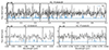 |
Fig. B.1. H |


H emission line properties.
Appendix C: PDR models of CH
As in previous papers by the PDRs4All team, we modeled the PDR component of d203-506 using the Meudon PDR code (Le Petit et al. 2006). We analyzed the same output model presented by Berné et al. (2023) to interpret the presence of CH in this disk. This models adopts G0 = 2×10⁴ and nH = 107 cm−3. The specific hydrocarbon chemistry is presented in Goicoechea et al. (2025). Figure C.1 (upper panel) shows the basic physical structure of the PDR component. The middle panel shows the C+/C/CO transition zone and the predicted CH+, CH
 , and CH abundance profiles (with respect to H nuclei). The lower panel shows the accumulated column densities of CH+, CH
 , and CH as a function of depth into the disk PDR.
Close to the hot PDR surface, where n(H) ≥ n(H2), we predict that CH formation is dominated by reactions of atomic C(3P) with FUV-pumped, vibrationally excited H2(v), which is a very endoergic reaction5, about ∼11,000 K when v = 0 (e.g., Dean et al. 1991). This hot chemistry leads to the first CH abundance peak in Fig. C.1. In addition, reactions of electronically excited neutral carbon atoms (e.g., C(1S) and C(1D), as detected by Haworth et al. 2023; Goicoechea et al. 2024) with H2 likely contribute to enhance the production of CH. These reactions are highly exothermic (e.g., González-Lezana 2007), but they are currently not included in our models or in other irradiated disk models. Still, we expect that most of the CH column density arises from deeper layers within the molecular PDR, beyond the CH abundance peak. In these regions, CH formation is driven by the dissociative recombination of CH
 ions, which either directly produce CH or yield CH2 molecules that subsequently react with H atoms to form CH.
This photochemical model predicts a total CH column density N(CH) ≲1014 cm−2 across the PDR, and gas temperatures varying from ∼4000 K at the rim of the PDR to several hundred in the more FUV-shielded layers. These temperatures are broadly consistent with the excitation temperature derived using PAHTATmol. Still, non-LTE excitation models will be required to accurately determine the true IR-emitting CH column density and its precise location within the disk PDR.
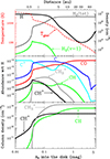 |
Fig. C.1. Predicted physical (roughly vertical) structure of the PDR component of d203-506. Upper panel: Gas density and temperature profiles as a function of depth into the PDR. Middle panel: Abundance profiles of selected species. Lower panel: Column densities as a function of depth into the PDR of small hydrocarbons detected by JWST in d203-506 (see also Berné et al. 2024; Zannese et al. 2025). |
All Tables
Molecules included in PAHTATmol, with references to the spectroscopic parameters used to compute the emission spectra.
All Figures
|
Fig. 1. Bottom panel: PAHTATMOL shifted fit result (blue curve) on the NIRSpec f290lp filter spectrum of d203-506 (black curve). The different colors at the bottom of the panel show the inverted individual molecular spectra, and a dotted magenta line shows the atomic and H2 emission lines. Upper panel: Model residual (observed spectrum minus the model). |
| In the text | |
|
Fig. 2. Near-infrared CH rovibrational emission in d203-506. The continuum-subtracted observations are shown in black, and the CH model–offset for clarity–is shown in orange. The dotted magenta lines indicate model spectra for additional species. |
| In the text | |
|
Fig. 4. H |
| In the text | |
|
Fig. 3. IR JWST images of d203-506. Top left: NIRCam F182M (broad filter centered at 1.82 μm). Top right: NIRCam F212N (H2 1-0 S(1) emission). Bottom left: NIRSpec CH emission map, continuum subtracted. Bottom right: NIRSpec Q(1,0) H |
| In the text | |
|
Fig. A.1. d203-506 NIRSpec spectrum in black. Each NIRSpec filter wavelength coverage is shown below the spectrum. |
| In the text | |
|
Fig. B.1. H |
| In the text | |
|
Fig. C.1. Predicted physical (roughly vertical) structure of the PDR component of d203-506. Upper panel: Gas density and temperature profiles as a function of depth into the PDR. Middle panel: Abundance profiles of selected species. Lower panel: Column densities as a function of depth into the PDR of small hydrocarbons detected by JWST in d203-506 (see also Berné et al. 2024; Zannese et al. 2025). |
| In the text | |
Current usage metrics show cumulative count of Article Views (full-text article views including HTML views, PDF and ePub downloads, according to the available data) and Abstracts Views on Vision4Press platform.
Data correspond to usage on the plateform after 2015. The current usage metrics is available 48-96 hours after online publication and is updated daily on week days.
Initial download of the metrics may take a while.