| Issue |
A&A
Volume 696, April 2025
|
|
|---|---|---|
| Article Number | A206 | |
| Number of page(s) | 25 | |
| Section | Extragalactic astronomy | |
| DOI | https://doi.org/10.1051/0004-6361/202451464 | |
| Published online | 25 April 2025 | |
A MaNGA view of isolated galaxy mergers in the star-forming main sequence
1
Instituto de Física, Pontificia Universidad Católica de Valparaíso, Casilla, 4059 Valparaíso, Chile
2
Departamento de Física Teórica y del Cosmos, Edificio Mecenas, Campus Fuentenueva, Universidad de Granada, 18071 Granada, Spain
3
Instituto Carlos I de Física Teórica y Computacional, Facultad de Ciencias, Universidad de Granada, 18071 Granada, Spain
4
Université Côte d’Azur, Observatoire de la Côte d’Azur, CNRS, Laboratoire Lagrange, 06000 Nice, France
⋆ Corresponding authors: This email address is being protected from spambots. You need JavaScript enabled to view it.
Received:
11
July
2024
Accepted:
13
February
2025
Abstract
Context. There are still many open questions in the complex process of galaxy evolution during interactions, as each stage is characterized by different periods of star formation.
Aims. We aim to better understand the processes triggered in galaxies by interactions. We consider low-density environments in which in-situ interaction between the members is the main process that drives evolution.
Methods. In this work we carried out an analysis of star-formation and nuclear activity at different stages during a galaxy merger identified in isolated systems (isolated galaxies, isolated pairs, and isolated triplets) using integral field spectroscopy from the Mapping Nearby Galaxies at Apache Point Observatory (MaNGA) project. We classified galaxies into close pairs, pre-mergers, mergers, and post-mergers (including galaxies with post-starburst spectroscopic features) for a total sample of 137 galaxies. We constrained their star formation history from spectro-photometric SED fitting with Code Investigating GALaxy Emission (CIGALE), and used spatially resolved WHAN diagrams, with other MaNGA data products to explore whether there is any connection between their physical properties and their merging stage.
Results. In general, galaxies show characteristic properties intrinsically related to each stage of the merger process. Galaxies in the merger and post-merger stages present higher star-formation activity (measured by their integrated sSFR). In the merger stage, the fraction of strong AGN spaxels is comparable to the fraction of spaxels with pure star-formation emission, with no difference between the AGN activity in close pairs and strongly interacting galaxies with the same stellar mass.
Conclusions. Our results support the scenario where galaxy interactions trigger star formation and nuclear activity on galaxies. Nonetheless, the AGN has a minor role in quenching galaxies following a merger, as AGN feedback might not have had sufficient time to inhibit star formation. In addition, we found that the quenching process in post-merger galaxies with post-starburst emission happens outside-in, which is an observational proof of the effect of interactions on the quenching process. The transforming processes after a recent major galaxy interaction may happen slowly in isolated environments, where the system evolves in a common dark matter halo with no perturbation from external galaxies.
Key words: galaxies: evolution / galaxies: formation / galaxies: general / galaxies: interactions / galaxies: star formation
© The Authors 2025
 Open Access article, published by EDP Sciences, under the terms of the Creative Commons Attribution License (https://creativecommons.org/licenses/by/4.0), which permits unrestricted use, distribution, and reproduction in any medium, provided the original work is properly cited.
This article is published in open access under the Subscribe to Open model. This email address is being protected from spambots. You need JavaScript enabled to view it. to support open access publication.
1. Introduction
Galaxy interactions and mergers play a fundamental role in the evolution of galaxies, and intrinsically influence their shape, growth, and physical properties. The gravitational interactions between galaxies, which usually form structures such as tidal tails (Toomre & Toomre 1972; Mihos & Hernquist 1996), and the friction between the gas and dust have major effects on the galaxies involved. Due to their nature, these processes are chaotic, which makes them difficult to understand physically. The result of a galaxy merger depends on a wide variety of parameters such as relative size and/or composition or galaxy morphology, and kinematic parameters such as collision angle and relative velocity, thus necessitating studies of galaxy interactions in both controlled environments and simulations (Athanassoula et al. 1999; Bournaud et al. 2005; Di Matteo et al. 2007; Lotz et al. 2010; Moster et al. 2011), but also using photometric and spectroscopic observational data (Bergvall et al. 2003; Lotz et al. 2004; Lin et al. 2007, 2008; Michiyama et al. 2016; Ellison et al. 2019, 2022; Pearson et al. 2019; Chang et al. 2022; Grajales-Medina et al. 2023), which all together provide a global picture to investigate these processes.
Over recent decades, many different studies have shown that these evolutionary mechanisms are responsible for changes in the internal physical properties of galaxies, in particular the enhancement of star formation, which strongly implies a connection between galaxy interactions and the birth of stars (Roukema et al. 1997). Star formation during galaxy interactions may occur in particular regions through abrupt bursts in the regions where galaxy interactions occur (Toomre & Toomre 1972; Kennicutt et al. 1987; Barton et al. 2000, 2007; Barton Gillespie et al. 2003; Lambas et al. 2003; Bell et al. 2006; Robaina et al. 2009; Jogee et al. 2009; Pearson et al. 2019; Renaud et al. 2022). Additionally, star-forming regions can emerge in gas clouds within tidal tails or in the bridge of material between galaxies (Naab et al. 1999, 2006a; de Mello et al. 2008; Boquien et al. 2009, 2010, 2011; Duc et al. 2013; Ji et al. 2014; Dumont & Martel 2021; Pasha et al. 2021).
These violent interactions trigger and accelerate the processes of star formation in galaxies. Galaxies that have suffered a recent interaction transit from a state of starburst or enhanced star formation (e.g. Joseph & Wright 1985; Knapen & Cisternas 2015; Mesa et al. 2021; Trevisan et al. 2021; Laufman et al. 2022) to a quenching state, occur faster than in normal (non-interacting) galaxies (Faber et al. 2007; Peng et al. 2010; Bell et al. 2012; Bergvall et al. 2016; Pearson et al. 2019). It has been also observed that, in addition to an increment of star formation, galaxy interactions may trigger the nuclear activity of galaxies, which might also be connected to star-formation quenching by active galactic nuclei (AGNs) feedback processes (e.g., Sanders & Mirabel 1996; Alonso et al. 2007; Darg et al. 2010; Weigel et al. 2018; Ellison et al. 2019).
In particular, AGN is one of the main drivers for the transition from star-forming disk to passive spheroidal galaxies (Kauffmann et al. 2003). In an AGN, the supermassive black hole (SMBH) that grows through mass accretion at the centre of massive galaxies releases large amounts of energy into its surroundings, as well as into the galaxy itself Magorrian et al. (1998), Ferrarese & Merritt (2000), Marconi et al. (2004), Kormendy & Ho (2013). How the energy accretion or AGN feedback (the posteriori re-deposition of energy and momentum into the interstellar medium through outflows and radiation) generate changes in galaxies, such as in the stellar populations in the bulge and outgrowth (Schawinski et al. 2007; Silverman et al. 2008; Mullaney et al. 2015; Sánchez et al. 2018; Lacerda et al. 2020) or significant increment in the star formation rate (SFR) of galaxies (Koss et al. 2011; Santini et al. 2012; Ellison et al. 2016; Woo et al. 2020), are some of the currently unanswered topics. There is some evidence that major mergers are the main driver of high luminosity AGNs (Ellison et al. 2011; Ramos Almeida et al. 2012; Kaviraj et al. 2015). Moreover, AGNs in interacting systems, through AGN feedback, may have an important role in regulating star formation in these interacting systems, but this argument is still under debate due to the recent incorporation of integral field unit (IFU) spectroscopy. Some studies reveal that there is a correlation between these phenomena (Ellison et al. 2011, 2013; Lackner et al. 2014; Satyapal et al. 2014; Goulding et al. 2018), while others contradict it (Cisternas et al. 2011; Villforth et al. 2017; Marian et al. 2019; Silva et al. 2021).
Because of the aforementioned issues, many open questions in the complex process of galaxy evolution during interactions still remain, as each stage is characterized by different periods of star formation (e.g., Solanes et al. 2018; Hopkins et al. 2008; Rodriguez-Gomez et al. 2015). In addition, the bibliography distinguishes between two main types of interactions depending on the presence of cold and molecular gas: ‘wet’ mergers, which are mergers of galaxies where a galaxy contains a substantial amount of gas to form stars; and ‘dry’ mergers, which are mergers of galaxies with a low gas content do not trigger starbursts or significant star formation (Naab et al. 2006b; Lin et al. 2010; Eliche-Moral et al. 2011). The types of interaction also depend on the mass ratio between the galaxies: minor merger, when the stellar mass of the companion is typically less than 1/10; and major merger, when the companion galaxy has a similar stellar mass (Lambas et al. 2012; Di Teodoro & Fraternali 2014). Therefore the different stage of the interactions may present different properties in the galaxies depending of the type of merger (Hopkins et al. 2010; Méndez-Abreu et al. 2014; Weston et al. 2017; Chang et al. 2022). The analysis of galaxy interactions might be much better understood if low-density environments are considered, making in situ interaction between the members the main process driving their evolution, with minimal contamination from other external environment processes that may happen, for instance, within a galaxy cluster (Henderson & Bekki 2016). For this reason, the Sloan Digital Sky Survey (SDSS) catalogues of Isolated Galaxies (SIG), Isolated Pairs (SIP), and Isolated Triplets (SIT) presented in Argudo-Fernández et al. (2015) are ideal to investigate these processes. Moreover, as is shown in Vásquez-Bustos et al. (2023), we can easily identify the presence of galaxy interactions in isolated systems with high values of the tidal strength parameter (Qtrip > −2 for the SIT). Regarding this question, in this work we carry out an analysis of star-formation and nuclear activity at the different stages during a galaxy merger identified in isolated systems (isolated galaxies, isolated pairs, and isolated triplets). To better understand the physical processes that occur in the galaxies, we used IFU spectroscopy from the MaNGA (MApping Nearby Galaxies at APO; Bundy et al. 2015; Drory et al. 2015) survey.
This study is organised as follows. In Sect. 2 we explain how we selected galaxies at different stages of the merger process from the SIG, SIP, and SIT catalogues that have available MaNGA data. The methods we used to constrain the star-formation histories (SFH) from spectro-photometric spectral energy distribution (SED) fitting, as well as emission line diagnostic diagrams to explore nuclear activity, are presented in Sect. 3. Our results and their corresponding discussion are presented in Sects. 4 and 5, respectively. A brief summary and the conclusions of this analysis can be found in Sect. 6. Throughout the study, a cosmology with ΩΛ0 = 0.7, Ωm0 = 0.3, and H0 = 70 km s−1 Mpc−1 is assumed.
2. Data and the sample
2.1. MaNGA data
Integral field spectroscopy (IFS) provides a more complete understanding of the emissions in different regions and components of galaxies. In particular, optical IFS is helping us to understand the local versus global universal relations in galaxies (Barrera-Ballesteros et al. 2016) and, for instance, how low ionisation emission-line regions are not only found in the nuclear regions of galaxies (Belfiore et al. 2016).
For this study we used spectroscopic data from the MaNGA survey, which provides IFU data products for 10.000 galaxies in the local universe (z < 0.15) as part of the SDSS-IV legacy survey (Blanton et al. 2017; Abdurro’uf et al. 2022). MaNGA uses hexagonal fibre bundles, each containing between 19 and 127 spectroscopic fibres, which ensures the delivery of a minimum spatially resolved spectrum coverage of 1.5 effective radius per galaxy in the primary sample, and 2.5 effective radius for the secondary sample. It also covers a spectral range from 3600 Å to 10 300 Å, with a resolution of R = 2000. MaNGA data products include sky-subtracted spectrophotometrically calibrated spectra and rectified three-dimensional data cubes (Law et al. 2016, 2021), and high level data products, including stellar kinematics (velocity and velocity dispersion), emission-line properties (kinematics, fluxes, and equivalent widths), and spectral indices (Bruzual 1983; Burstein et al. 1984; Faber et al. 1985; Poggianti & Barbaro 1997; Gallazzi et al. 2005, e.g. D4000 and the Lick indices,). More information about the MaNGA data products and its pipeline can be found in Westfall et al. (2019) and Belfiore et al. (2019). The MaNGA dataset can be accessed via Marvin1 tools (Cherinka et al. 2019).
For this study we used Hα and Hβ emission line maps, with the Dn 4000 map and the spectrum in each spaxel, to constrain the star-formation history, as explained in Sect. 3.4. We also used the [NII] emission map with the equivalent widths WHα and WNII to create diagnostic diagrams of the nuclear activity, as explained in Sect. 3.5.
2.2. Interacting galaxies in isolated systems
As introduced in Sect. 1, for this study we used the SIG, SIP, and SIT catalogues compiled by Argudo-Fernández et al. (2015) based on the SDSS survey data. The catalogues contain 3702 isolated galaxies, 1240 isolated pairs, and 315 isolated triplets, respectively, in the local Universe (z ≤ 0.080). The systems are isolated, with no nearest neighbours within a Δv ≤ 500 km s−1 line-of-sight velocity difference with a spatial projected radius of the field of 1 Mpc. Galaxies in the SIG, and central galaxies in the SIP and SIT (named as A galaxies in Argudo-Fernández et al. 2015), are brighter than an r-band apparent magnitude, mr = 15.7. This allows us to search for satellite galaxies up to two magnitudes fainter within the spectroscopic completeness limit of the SDSS (mr = 17.7). Therefore satellite galaxies are fainter, and also generally less massive, than central galaxies. Galaxies in the SIP and SIT are physically bound at a projected distance up to d ≤ 450 kpc within a Δv ≤ 160 km s−1 line-of-sight velocity difference with respect to the central (the brightest) galaxy. Argudo-Fernández et al. (2015) also provide a quantification of the local and the large-scale environment for galaxies in the SIG, SIP, and SIT using local number densities and tidal strength parameters. We refer to Argudo-Fernández et al. (2015) for more information about the compilation of the catalogues. In addition to the aforementioned catalogues, we used a non-public sample of 12 isolated mergers that were removed when compiling the SIG (hereafter the SIM, following the naming format of the samples from Argudo-Fernández et al. 2015). We used the Marvin tools to access to the MaNGA dataset, and we found that 54 SIT galaxies, 156 SIP galaxies, 348 SIG galaxies, and 6 SIM galaxies have available data products. We note that, in the case of SIP and SIT samples, MaNGA observations for all the galaxies belonging to the same system are not always available. Since we are not interested on studying interactions within the same system, which is beyond the scope of this work and would be limited to a few individual systems, we used these samples to select galaxies at different interaction stages to explore the impact of the interaction on the galaxies that have available MaNGA data.
To consider the level of interaction between all members in the SIP and SIT, independently of the available MaNGA data, we used the tidal strength parameter Q. As presented in Vásquez-Bustos et al. (2023), isolated triplets with Qtrip > − 2 show compact configurations due to interactions happening in the systems. In particular, triplets with Qtrip > − 0.45 present on-going mergers and strong interactions (Vásquez-Bustos et al. 2023). Taking into account that the sample of merging and/or strong interacting galaxies in the SIT is small (37 triplets, without considering the availability of IFU data), we followed the same selection criteria to identify interacting galaxies in the SIP, using in this case the QA parameter, as defined in Argudo-Fernández et al. (2015). Given that the SIG, SIP, and SIT were selected homogeneously following the same isolation criteria, we also looked for visually disturbed isolated galaxies in the SIG. We performed a visual inspection of the SDSS three-colour images of the galaxies in the SIT, SIP, SIG, and SIM, to identify and classify the level of interaction. To identify possible features that are fainter than SDSS images, we also used three-colour images from Pan-STARRS 1 (Chambers et al. 2016) for a better visualisation of the structure of the galaxies. We also used spectroscopic MaNGA data to identify possible post-starburst galaxies, since these galaxies might have suffered a recent past interaction. The details of the identification of the galaxies at different interaction stages are presented in Sect. 3.1.
3. Methodology
3.1. Merging stage
To better understand the complex processes that happen during galaxy mergers, it is necessary to divide the galaxies into different stages of interaction, starting from close pairs, through the merging process, and to the post-merger scenario. For instance, star formation can reach its maximum during a pre-merger or merging period or rapidly decay over a short timescale after a major merger event. We classify the galaxies in the following categories according to their merging stage as detailed below:
-
Close pair (CP): Close pairs of galaxies in the SIT and the SIP with projected distance d ≤ 100 kpc (see Fig. 1). For these galaxies no signs of interactions between the members, such as tidal arms and tails or deformations, is detectable from a visual inspection. Therefore this sample can be used as a control sample for the other categories, where signs of interaction are visually present. An example of a galaxy in this category is shown in Fig. A.1.
-
Pre-merger (PrM): A low to mild level of interaction is visibly appreciable between physically bound galaxies in the SIP and SIT, with slight deformations of the spiral arms (in the case of late-type galaxies), with a projected distance d ≤ 100 kpc and local tidal strength QA < − 2 (within the left-hand side of the shaded area in Fig. 1). Under this category, visible tidal tails and bridges of materials between galaxies can be observed, however the two galaxies can be independently identified, therefore the process of merging of the nuclei has not yet started. We note that the galaxies in this category may have undergone an interaction process that deformed them a long time ago. An example of a galaxy in this category is shown in Fig. A.2.
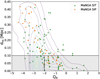
Fig. 1. Projected distance to the nearest companion dnc, in Mpc, with respect to the tidal strength of the central galaxy on the system QA. Contour lines correspond to all the galaxies in the SIP and SIT; green triangles and orange hexagons indicate galaxies in the SIT and SIP, respectively, from MaNGA data. The horizontal solid black line delimits the grey shaded area with dnc ≤ 100 kpc that we use to delimit close pairs. Within this area, the vertical solid black line at QA = − 2 is used to identify interacting galaxies, following Vásquez-Bustos et al. (2023).
-
Merger (M): This category covers the stage where galaxy nuclei merge. Within this category, large deformations in most of the visible regions of galaxies, accretion of matter from one galaxy to another, as well as tidal arms and bridges can be visually observed in the optical SDSS images. For these cases, we found that both galaxies could be present in a single MaNGA field of view (FoV). An example of a galaxy in this category is shown in Fig. A.3.
-
Post-merger (PsM): This category covers the final stages of an interaction. This sample is composed of galaxies in the SIG and the SIM that have visible signs of interaction but without the presence of an observable close companion galaxy. We also included some galaxies with post-starburst spectroscopic signatures. The criteria followed to select these galaxies is explained in Sect. 3.2. An example of a galaxy in the PsM category is shown in Fig. A.4.
We note that each point in Fig. 1 does not always correspond to a pair of galaxies that belong to the same system. It may correspond to a single galaxy in the case of SIP and SIT systems with MaNGA products for only one galaxy. The sample of interacting galaxies at different merging stages is composed of a total of 137 galaxies. The number of galaxies for each category is shown in Table 1, while the number of central and satellites for each merger classification is presented in Table 2.
Number of galaxies at each merging stage.
Number of central and satellite galaxies at each merging stage.
3.2. Identification of post-merger galaxies
This category is mainly composed of galaxies in the SIG and the SIM that have signs of a recent interaction but not observable companion. We also visually searched for shells signatures around since these are indicators of recent interactions or that galaxies have undergone a nucleus merger process (Mancillas et al. 2019; Balcells et al. 2001; Petersson et al. 2023). In general, this category might be complex to identify, especially in the case of early-type galaxies, since the low surface brightness features might not be visible in the optical SDSS images. Therefore we considered other observational aspects that might be related to a recent merger event.
Some studies claim that lenticular or S0 galaxies might be the result of a major merger event between two spiral galaxies of unequal masses (Bekki 2001; Eliche-Moral et al. 2012, 2018; Querejeta et al. 2015a,b). However, there are other mechanisms involved in the formation of lenticular galaxies, for example internal secular evolution and environmental processes, in particular for the formation of intermediate to low mass lenticulars (Tapia et al. 2017). Therefore, a selection based on optical morphology might introduce a strong bias. On the other hand, some works argue that a high percentage of post−starburst (PSB) galaxies (sometimes also referred to as E+A or K+A galaxies, i.e. galaxies that have recently experienced an episode of intense star formation that was rapidly truncated) might be due to a recent interaction that suddenly quenched their star formation (Goto 2005; Snyder et al. 2011; Wilkinson et al. 2022; Ellison et al. 2022). Taking into account the fact that we are working with isolated galaxies, we consider that the most probable reason for the presence of PSB spectral signatures in these galaxies is that they have undergone a recent past interaction (Sazonova et al. 2021).
We identified PSB galaxies using traditional selection methods consistent with the analysis of the Hα equivalent width (in Å) with respect to the summed stellar continuum indices HδA and HγA diagnostic diagram (Zheng et al. 2020). These spectroscopic measurements are available in the MaNGA data products. For simplicity, we considered the products from the central spaxel (usually corresponding to the galaxy nucleus) to identify candidate PSB galaxies, and then used the spatially resolved information to analyse them in more detail. For homogeneity, we reproduced the diagnostic diagram for all the galaxies in our samples (see Fig. 2), including galaxies in the SIP and SIT since they might have suffered a previous merger event (not related to an interaction with the current galaxies in the system). The PSB candidate galaxies are those enclosed in the shaded area of the diagram, known as the PSB region (Goto et al. 2003; Quintero et al. 2004; Balogh et al. 2005). We found seven galaxies (three SIG galaxies, three SIP galaxies, and one SIT galaxy): 8088-3704, 12067-3701, 8981-12705, 8483-12702, 8555-3701, 11955-6103, and 9194-3702. Figure 3 shows the spatially resolved PSB diagnostic diagrams for these galaxies. The PSB emission is mainly present in the centre of the galaxies but we also found some spatial distribution outside the centre, which is also expected and in agreement with similar analyses of MaNGA galaxies (Chen et al. 2019; Li et al. 2023). We therefore included these seven galaxies in the PsM category.
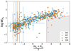 |
Fig. 2. Post-starburst diagnostic diagram (spectral index distributions Hα equivalent width vs. |

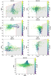 |
Fig. 3. Spatially resolved PSB diagram (Hα equivalent width vs. |

3.3. Galaxy morphology
The classification of the galaxies at different merging stages is independent of their morphology, that is, of whether the galaxy is early or late type. Our visual classification is based on the presence (or absence) of a close companion and/or interaction features (tidal tails and shells, for instance). In order to take into account the morphological type of the galaxies in our sample as a function of their merging stage, we used the morphological classification in Domínguez Sánchez et al. (2018), hereafter DS18, which provides deep-learning-based morphological classification for ∼670 000 galaxies using SDSS data. DS18 provided a T-Type classification, in a continuous scale, related to the Hubble morphological type, after using the visual morphological classification from the Galaxy Zoo project2, in particular from the Galaxy Zoo 2 (GZ2, Willett et al. 2013) catalogue and the morphological classification by Nair & Abraham (2010), to train and test their deep learning models. The T-Type parameter ranges from −3 to 10, where T-Type ≤ 0 corresponds to early-type galaxies (i.e. elliptical and lenticular galaxies), and positive values to late-type galaxies, with T-Type = 10 for irregular galaxies.
We found that 134 galaxies in our sample have a morphology classification in DS18. The remaining three galaxies are early type, based on a visual revision of the optical SDSS images. We only considered if the galaxies are classified as late type (including irregulars) or early type (considering ellipticals and lenticulars) using DS18 morphology. DS18 also provided the parameter Pmerger as the probability that a galaxy presents merger morphology, and the probability that it is a lenticular (or S0) galaxy (PS0), where a value of PS0 > 0.5 for a galaxy with T-Type ≤ 0 indicates that it is a lenticular galaxy.
3.4. Spectro-photometric spectral energy distribution fitting
We combined photometric and spectroscopic data to derive the spectral energy distribution (SED) of the 137 galaxies in our sample. The SED of a galaxy is a powerful tool for constraining key physical properties of the unresolved stellar populations, such as their SFH. We used the Code Investigating GALaxy Emission3 (CIGALE; Burgarella et al. 2005; Noll et al. 2009; Boquien et al. 2019), which allows us to perform the spectro-photometric SED fitting. CIGALE models the SED of galaxies by considering the energy balance, that is, by taking into account the UV/optical dust attenuation, to derive the SFR, recent star formation, age, stellar masses, and dust attenuation in galaxies, among other physical properties and parameters of the SFH, following a Bayesian analysis (e.g. Buat et al. 2011; Giovannoli et al. 2011; Boquien et al. 2014; Ciesla et al. 2017; Yuan et al. 2018; Boquien et al. 2022). The results of the spectro-photometric SED fitting for each spaxel allow us to explore the spatially resolved SFH through the SFR, and other properties such as the stellar mass.
To get the required CIGALE input data, we used the Marvin tool. From the extensive MaNGA data products, we selected the maps of the Hα and Hβ emission lines, as well as the Dn4000 break spectral index, as defined in Balogh et al. (1999), for a more accurate estimation of the physical properties. Figure 4 shows these products for an example merger galaxy, 8241-12705, in our sample. In combination with spectroscopy, we defined custom photometric filters to account for the continuum, avoiding the main emission lines in the optical range of the MaNGA spectra, in order to compute the stellar mass. We defined our filters using a rectangle response function with a width that provided enough signal to noise (S/N) ratio, even in the external regions of galaxies covered by the MaNGA FoV. The information about each filter is summarised in Table 3. An example of the selected filters applied to a randomly selected high and low S/N ratio spaxel in the FoV of the merger galaxy 12483-12704 is shown in the upper and lower panels of Fig. 5, respectively. Figure 6 shows a map of the S/N ratio for each filter for the same galaxy.
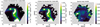 |
Fig. 4. MaNGA DAP products used as spectroscopic inputs in CIGALE to estimate physical properties from SED fitting for the galaxy 8241-12705 as example. From left to right: Hα emission line map, Hβ emission line map, and Dn4000 spectral index map. |
Custom filters defined for the SED fitting.
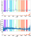 |
Fig. 5. Custom filters over a high and low S/N MaNGA spectra. We show the spectra in two different spaxels for the MaNGA galaxy 12483-12704, one with high S/N (upper panel) and another with low S/N (lower panel) selected from the MaNGA DAP datacube, for comparison. In both panels, the spectra are represented by solid blue lines that cover the full range of the MaNGA spectra, from 3600 to 10 000 Å. The corresponding error is represented by an orange line in the sub-panels. Colour regions show the custom filter wavelength range, with purple, blue, light blue, cyan, green, yellow, orange, and red corresponding to the M3992, M4542, M5446, N6097, N6908, O7473, O8281, and O9265 filters, respectively. The central wavelength that corresponds to each filter is represented by red circles. |
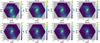 |
Fig. 6. Signal-to-noise ratio maps for each custom filter for the merger galaxy 8241-12705. From the upper left to lower right, S/N maps for filters M3992, M4542, M5446, N6097, N6908, O7473, O8281, and O9265, respectively. |
We chose a delayed SFH that considers a recent burst or quench episode as defined in Ciesla et al. (2017). This is the simplest SFH model for interacting galaxies as it easily accounts for the presence of a recent variation in the SFR due to a starburst episode or a rapid transition to a quench state (Ciesla et al. 2016). This module is provided in CIGALE as sfhdelayedbq (Boquien et al. 2019) following the equation
 (1)
(1)
where t0 is the age when is allowed, a rapid increment or decrease in the SFH, rSFR is defined as the ratio of the SFR after or before the t0, and τ represents the time at which the SFR peaks.
In the creation of the SED models for the SFH, we used the BC03 models of single stellar populations by Bruzual & Charlot (2003), considering a Salpeter initial mass function (IMF) Salpeter (1955), with a stellar metallicity value of Z = 0.02 (solar metallicity) for the modelling of an unattenuated stellar emission, and continuum and line nebular emission. We considered a modified Calzetti et al. (2000) starburst attenuation model such as dustatt_modified_staburst, with a Leitherer et al. (2002) curve extended between the Lyman break and 150 nm, and with a flexible attenuation curve (Noll et al. 2009).
Since we do not have data in the mid- or far-infrared (i.e. no band that is sensitive to dust emission), and to speed up the computation time of the spaxel-by-spaxel SED fitting, we did not select any dust emission model in the computation of the modelled SEDs. We note that, in addition to the synthetic bands, we also fit Hα, Hβ, and D4000. In this case, CIGALE uses Hα/Hβ as a tracer of the attenuation, and therefore it serves a similar role as the dust would in the construction of the modelled spectra. A total of 1749600 SED models were created using the parameters and values summarised in Table 4. With this configuration, the mean computational time to perform the spaxel-by-spaxel SED fitting is ∼2 hours/galaxy4 (for about 6850 total spectra for 137 galaxies).
Parameters used in CIGALE to model the SFH.
3.5. Analysis of the nuclear activity
For an analysis of the nuclear activity in galaxies, it is useful to use diagnostic emission line diagrams. These are an accurate empirical method to classify galaxies in terms of their emission in relation to the different mechanisms for gas ionisation. The most commonly used diagnostic diagrams for nearby galaxies are the Baldwin, Phillips, and Terlevich (BPT) diagrams (Baldwin et al. 1981; Kewley et al. 2006). Based on emission line ratios of [O III]/Hβ versus [N II]/Hα, [S II]/Hα, and [O I]/Hα, BPT diagrams allow us to classify galaxies into galaxies with a star forming nucleus (SFN), AGN Seyfert galaxies, low-ionisation (nuclear) emission-line galaxies, or LI(N)ERs, and passive galaxies.
MaNGA spectroscopy allows us to reproduce spatially resolved diagnostic diagrams, which consider the information from each spaxel. However, using BPT diagrams, the spectra only becomes classified if it meets the criteria in all three diagrams. Even selecting the most relaxed criterion ([O III]/Hβ versus [N II]/Hα), it depends on the emission in four lines, where [O III] and Hβ might be weak, which limits the area where we can analyse the galaxy. A way to overcome this issue is using the [N II]/Hα WHAN diagram (Cid Fernandes et al. 2011), which is able to analyse weak line galaxies, providing a more complete view of the diverse activity in different regions of the MaNGA galaxies that could not be explored using the BPT diagram due to the absence of absorption lines, for example.
The WHAN diagnostic diagram separates the weak AGNs from fake AGNs, named as retired galaxies (RGs) from LI(N)ERs, which enables a more complete analysis of regions where heating of the ionised gas is the result of old stars, rather than star-formation or AGN activity. We can also classify stellar activity into pure star-forming (PSF) or passive galaxies (PG), which are slightly different from the RGs, though PG are closely related to RGs, being an extreme case of stellar activity. Cid Fernandes et al. (2011) classified the different categories with respect to the values of log[NII]/Hα, WHα, and WNII, in the following way:
-
Pure star-forming galaxies (PSF): log[NII]/Hα < −0.4 and WHα > 3 Å;
-
Strong AGN (sAGN): log[NII]/Hα > −0.4 and WHα > 6 Å;
-
Weak AGN (wAGN): log[NII]/Hα > −0.4 and 3 < WHα < 6 Å;
-
Retired galaxies (RG): WHα < 3 Å;
-
Passive galaxies (PG): WHα < 0.5 Å and WNII < 0.5 Å.
Both BPT and WHAN diagrams can be computed using the Marvin tools. In particular, we developed the visualisation tool described in Appendix B, which uses the functionality already implemented in Marvin, but it is specifically designed to also explore the intermediate areas between adjoining WHAN categories, which allows us to investigate transition processes in the diverse stellar population within different regions of the galaxies. We show the WAHN diagnostic diagram and map for galaxy 8241-12705 as an example in Fig. 7. In combination with the spatially resolved SFR from SED fitting, we used the resolved WHAN diagrams to investigate whether there is any relation between AGN activity and star formation in our sample of close pairs and/or mergers. The level of agreement between the star formation from SED fitting and WHAN diagrams is presented in Sect. 4.1.
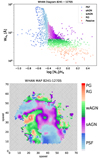 |
Fig. 7. Spatially resolved WHAN diagnostic diagram (upper panel) and map (lower panel) for the merger galaxy 8241-12705. Each colour, and color gradient, corresponds to a WHAN category according to the legend and colourbar, respectively. The WHAN diagram and map were created using the public tool for the visualisation of the spatially resolved WHAN diagnotic diagram for galaxies in the MaNGA survey described in Appendix B. |
4. Results
4.1. Spatially resolved stellar populations
We used the results from the spectro-photometric SED fitting with CIGALE to create SFR and stellar mass surface density maps (Σ SFR and Σ M⋆, respectively). We also created maps of the resulting χ2, which provides a view of the statistical distribution of the goodness of the fit of the models we created to the observations (Boquien et al. 2019), so we can identify if there are any problems with the fitting. We can detect whether the maps we get are reliable (lower χ2 values and no doubtful structures are shown in the maps), or whether we need to increase the parameter space when creating the models. An example of the maps generated from the results of the SED fitting is shown in Fig. 8. In comparison with the S/N maps in Fig. 6, the spaxels with the smallest χ2 values (< 0.02) typically have a S/N of 20. An example of the SED fitting products, among others, for a galaxy in each merger stage is also shown in Appendix A. The resulting SFR and M⋆ from SED fitting was used to construct the SFR-M⋆ diagram for galaxies in our sample, as a function of the merging stage, as explained in the next section. In addition, to explore stellar population properties such as age or nuclear activity, we used the Dn(4000) parameter and the results of the WHAN diagrams for all the galaxies in our sample.
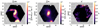 |
Fig. 8. Spatially resolved Σ SFR (left panel), Σ M⋆ (middle panel), and χ2 (right panel) maps from the results of the spectro-photometric SED fitting with CIGALE for the galaxy 8241-12705. The scale of the χ2 map is normalised to the maximum value. |
Besides using the Dn(4000) maps from the MaNGA Data Analysis Pipeline (DAP) as an input for CIGALE, we also used this parameter as the stellar population age indicator, which is small for younger stellar populations and large for older stellar populations. We used the divisory value of Dn(4000) = 1.67 following Mateus et al. (2006). Figure 9 shows the mean fraction of young (Dn(4000) ≤ 1.67) and old (Dn(4000) > 1.67) spaxels for each merger stage. We observe that, in general, merger and post-merger galaxies have a larger fraction of spaxels with young stellar populations, even galaxies in the PsM-PSB category. In addition, Fig. 10 shows the mean radial profile of Dn(4000) for each merger stage, with the results of the linear fit within 1.5 R/Reff5.
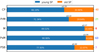 |
Fig. 9. Fraction of young and old spaxels for galaxies in each merger stage. We use the Dn(4000) parameter and the divisory value of Dn(4000) = 1.67 (as in Mateus et al. 2006) to separate between young (Dn(4000) ≤ 1.67, in blue) and old (Dn(4000) > 1.67, in orange) spaxels. The number of galaxies in each merger stage is indicated on the right-hand side, with text coloured as in Fig. 10. |
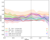 |
Fig. 10. Mean radial profiles of the Dn(4000) parameter with respect to R/Reff for all the galaxies in each merger stage. The radial profiles are represented in different colours for each merger stage according to the legend. Uncertainties are represented in the same colours at 1σ level. The slope, m, of the linear fit to the mean radial profile up to 1.5R/Reff (marked with a dashed vertical black line), with its corresponding uncertainties, are included in the legend for each merger stage. The number of galaxies in each merger stage is indicated in the lower right-hand corner, with text coloured as denoted in the legend. |
Similarly, Fig. 11 shows the percentage of spaxels in each WHAN category, for each merger stage. PsM and PsM-PSB galaxies show the largest fraction of PSF spaxels (∼65.1% and ∼51.7%) in comparison to M (∼43.2%), CP (∼47.2%), and PrM (∼47.3%). In the merger category, the percentage of AGN spaxels (sAGN + wAGN) is ∼10% higher than the percentage of PSF spaxels (43.2% versus 53.6%). In comparison, the fraction of PSF, AGN, and RG spaxels in CP galaxies is about one third in each case. The spatially resolved WHAN diagrams, and WHAN emission maps, for a galaxy in each merger stage are also shown in Appendix A.
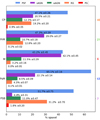 |
Fig. 11. Percentage of spaxels for each WHAN category for each merger stage. Blue colour bars represent the fractions of PSF spaxels, purple colour bars represent the fractions of sAGN spaxels, green colour bars represent the mean fractions of the wAGN spaxels, orange colour bars represent the fraction of spaxels classified as RG-like emission, and red colour bars represents the fraction of spaxels classified as PG-like emission, according to the WHAN diagnostic diagram. The number of galaxies in each merger stage is indicated in the right side, with text coloured as in Fig. 10. |
Figure 12 shows the level of agreement between the star formation obtained from SED fitting and from WHAN diagrams. The distribution of the specific star-formation rate (sSFR, defined as SFR/M⋆) surface density for spaxels that correspond to each WHAN category has some level of overlap. However, in general, PSF-classified spaxels present highest values of sSFR surface density, followed by the sAGN-, wAGN-, and RG-classifed spaxels, respectively. For all merger stages, the median values of the sSFR surface density are discernible at at least one sigma level for sAGN and RG WHAN classifications, while there is a large overlap for PSF and sAGN spaxels, especially for galaxies in the merger and post-merger stages. This is understandable considering the mix of processes occurring in galaxies at these stages.
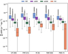 |
Fig. 12. Distribution of the sSFR surface density (ΣsSFR) for spaxels in each WHAN category for each merger stage (the number of galaxies in each category is indicated in parentheses). The distributions are shown in the form of box plots, with a different colour for each WHAN category as in Fig. 11. The median values of the distributions are represented by a horizontal line within the box plots, while the mean values are represented by a white circle. Outlier values (larger than 1.5× the inter-quartile range) are represented by black diamonds. The distribution for passive galaxies is not presented since the values of the ΣsSFR are null. |
4.2. Integrated SFR–M⋆ diagram
For each galaxy in our sample, we computed the integrated SFR and stellar mass considering the values in each spaxel to create an integrated SFR-M⋆ diagram. Figure 13 shows the values for the interacting and/or merger galaxies in our sample as function of their merger stage, including a differentiation for PSB galaxies within the PsM category. For reference, we added the values of the integrated SFR and stellar masses for all the MaNGA sample from the Pipe3D value-added catalogue (Sánchez et al. 2016b,a), as background contours, and the fit to the main sequence found by Argudo-Fernández et al. (2025), for SIG star-forming galaxies (dashed grey line). Galaxies in our sample are well distributed in the diagram, populating the main sequence and the quenched region. In particular, galaxies in the CP category can be found in both regions, PrM galaxies are scattered among the main sequence, with only one case in the quenched region, while M galaxies are found in the main sequence, with stellar masses within 10.1 log(M⊙)≲M⋆ ≲ 10.7 log(M⊙). Finally, PsM galaxies are found in two regions, where non-PSB galaxies are mainly located in the main sequence, while PsMs classified as PSBs can be found in the lower region of the main sequence, in the green valley, and in the quenched region. To quantify these differences, we also estimated the integrated sSFR and explored its relation with stellar mass using the sSFR–M⋆ diagram (see Fig. 146). The density distributions of the integrated properties are shown in Fig. 15 using violin plots. We used the distributions of the sSFR to explore whether there was any enhancement of star formation at any merger stage. In addition, the median values and uncertainties for each merging stage are presented in Table 5. We discuss the differences in the distributions for each merger stage in Sect. 5.3.
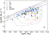 |
Fig. 13. Integrated SFR − M⋆ diagram for the 137 interacting galaxies in our sample. Galaxies classified as CP are represented by orange triangles, galaxies classified as PrM are represented by green hexagonal marks, M galaxies are represented by red stars, and galaxies classified as PsM are represented by blue and purple circles in the case of absence or presence of PSB emission, respectively. In the lower left-hand corner, we present a representative error, given by the mean value of the error of the integrated log SFRmean = 0.223 M⊙ yr−1 and the integrated log M⋆ mean = 0.097 M⊙. As reference, the contour backgrounds correspond to the integrated properties for all MaNGA galaxies from the Pipe3D value-added catalogue (Sánchez et al. 2016a,b), and the grey continuous line correspond to the ‘nurture’ free main sequence for star-forming galaxies derived by Argudo-Fernández et al. (2025). The dashed lines mark the locations with three, four, and seven times above the main sequence (along the SFR axis), respectively. |
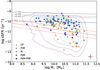 |
Fig. 14. Same as Fig. 13, integrated sSFR − M⋆ diagram for the 137 interacting galaxies in our sample. Galaxies classified as CP are represented by orange triangles, galaxies classified as PrM are represented by green hexagonal marks, M galaxies are represented by red stars, and galaxies classified as PsM are represented by blue and purple circles in the case of absence or presence of PSB emission, respectively. In the lower right-hand corner we present a representative error, given by the mean value of the error of the integrated log SFRmean = 0.24 M⊙ yr−1 and the integrated log M⋆ mean = 0.097 M⊙. As reference, the contours lines correspond to the integrated properties for all MaNGA galaxies from the Pipe3D value-added catalogue (Sánchez et al. 2016a,b). The grey continuous line corresponds to the ‘nurture’ free main sequence for star-forming galaxies derived by Argudo-Fernández et al. (2025). The dashed lines mark the locations with three, four, and seven times above the main sequence (along the SFR axis), respectively. The red continuous line corresponds to the fit to separate star forming from quenched galaxies in the Pipe3D sample, with its corresponding 1σ to delimit the green valley (dashed red lines). |
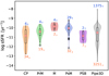 |
Fig. 15. Distribution of the integrated sSFR in the form of violin plots for each merger stage. The coloured area determines the density distribution for CP in orange, PrM in green, M in red, PsM in blue, and PSB in purple. For reference, the values of the integrated properties for all MaNGA galaxies (10010 galaxies) from the Pipe3D value-added catalogue (Sánchez et al. 2016a,b) have been added (in grey). The inner box on each violin plot is a representation of the interquartile range of the median (red dot) and its 95% of its confidence intervals. We also show the outlying points of the distributions (if any) as black open circles, which represent the atypical values for that category. The number of galaxies above and below the MS in Fig. 14 is indicated above and below the violin plots, respectively, while the total number of galaxies considered in each merger stage is presented in Table 1. |
Global physical properties for each merger stage category.
To relate the properties of the stellar populations for galaxies in our sample to their location in the SFR-M⋆ diagram, we also created different versions of the diagram as a function of the WHAN emission (see Fig. 16) and the Dn4000 spatial distribution, divided into young (Dn(4000) ≤ 1.67) and old (Dn(4000) > 1.67) stellar populations (as shown in Fig. 17). We discuss our results in Sect. 5.
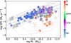 |
Fig. 16. Integrated SFR − M⋆ diagram for the 137 galaxies in the sample as in Fig. 13, with the point values as WHAN maps respectively for each galaxy. The colourbar represents the WHAN categories based on Cid Fernandes et al. (2011). The coloured hexagons indicate the merger stage for each galaxy in the diagram following the colour scheme in Fig. 13. The dashed lines mark the locations with three, four, and seven times above the main sequence (along the SFR axis), and 1/3, 1/4, and 1/7 times below the main sequence, respectively. |
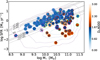 |
Fig. 17. Integrated SFR − M⋆ diagram for the 137 galaxies in the sample as in Fig. 16, but using maps of the age of the stellar populations instead of WHAN maps. The maps are divided into young blue degraded colour (for spaxels with Dn(4000) ≤ 1.67) and old orange degraded colour (for spaxels with Dn(4000) > 1.67) according to their Dn4000 parameter, respectively for each galaxy. |
5. Discussion
5.1. Classification of merger stage
The use of physical properties maps in combination with diagnostic maps, as well as emission maps, provides a comprehensive and complete picture of the physical processes that occur within galaxies. Thus it helps us to understand how the star-formation and/or quenching and AGN processes arise or evolve during galaxy interactions. We note that we found a discrepancy in the data provided by the WHAN maps, where they indicate sAGN ionisation features in areas where this emission is unlikely to occur and it would be more likely that the emission comes from stellar populations that are in the quenching process. This is shown in Fig. 12 as the overlapping distributions of sSFR surface density, however the median values are distinguishable at 1σ level. The maps also allowed us to perform a quality control check, where some galaxies were re-classified or removed. We removed some galaxies from the analysis in the case that the MaNGA FoV was too small, centred only on the bulge of the galaxy, or did not have good coverage of the galaxy. The final number of galaxies in each category is shown in Table 1.
We also compared our visual classification with other independent methods. We found that all galaxies classified as mergers in our sample have a mean probability pmerger = 0.78 of presenting merger morphology according to DS18. There are six M galaxies in our sample with MaNGA data, which is consistent with the expected number of merger galaxies in isolated systems (Grajales-Medina et al. 2023). We note that the selection criteria for the M category consider strong interactions including when the two overlapping galactic nuclei are still distinguishable in the optical image, which allows for the selection of dry mergers (i.e. merger of early-type galaxies with a lower content of cold gas). However, this type of merger is less common in low-density environments (Lin et al. 2010). None of the six M galaxies are composed of two early-type galaxies.
Other authors use non-parametric image predictors, such as Gini, M20, and Concentration–Asymmetry–Clumpiness (CAS) parameters (Conselice 2003; Lotz et al. 2004; Pawlik et al. 2016) to help in the identification of tidal tails and other interaction features (Nevin et al. 2019; Hernández-Toledo et al. 2023; Nevin et al. 2023). Taking advantage of the MaNGA DAP maps, we computed these parameters and applied them to the MaNGA FoV in the wide r-band, which is presented in Appendix C. A comparison of these parameters for the galaxies in our sample, with respect to the distribution of the same parameters for all MaNGA galaxies, is shown in Fig. C.1. We did not observe any clear trend in these parameters for our galaxies with respect to their merging stage. This might be due to the fact that MaNGA FoV usually covers from a 1.5 to a 2.5 effective radius, and interaction features are usually found at the outskirts of galaxies. However, we repeated the same analysis with the same morphology parameters for MaNGA galaxies provided by (Nevin et al. 2023) using r-band imaging data from SDSS-DR16. Again, we did not observe any clear relation with the parameters and the merger stage, however the galaxies used in this study in general showed higher A values than most of MaNGA galaxies, probably due to asymmetries that can be observed at the outskirts of galaxies in the SDSS imaging. Using both methods, we also observed some trends for galaxies in the PsM-PSB category. PsM-PSB galaxies are generally concentrated in regions with lower clumpiness values (S < 0.1), and have a lower inverse concentration index than galaxies at fixed M20 values. This means that light is more concentrated in the inner region of post-merger galaxies with spectral post-starburst features than galaxies with similar morphology, where the distribution of the light is also smoother. Moreover, two of the seven galaxies classified as PsM-PSB are lenticular galaxies, with a probability of being an S0 galaxy PS0 > 0.5 (mean PS0 = 0.8) in DS18, which is in agreement with the CAS parameters for these galaxies. We also found 13 CP galaxies with lenticular morphology, which are distributed in the same region of the CAS parameters where PsM-PSB galaxies are located (as shown in Fig. C.1). The incidence of lenticular galaxies in the PsM-PSB category is similar to CP galaxies, both larger than the other merger stages7. We conclude that isolated galaxies that have recently undergone a major merger event, which triggered PSB activity, present lenticular morphology, and therefore their morphology might be the result of the merger process. This formation scenario is in agreement with recent studies of the pathways for the formation of S0 galaxies, where merger-triggered formation becomes a more efficient mechanism in lower-density environments (Coccato et al. 2020, 2022; Chen et al. 2024).
5.2. Spatially resolved stellar populations
After analysing the spatially resolved SFR and diagnostic diagrams introduced in Sect. 3, with the MaNGA data products as described in Sect. 4, we found some relations between the physical properties we considered in this study and their merging stage. In general, the spatially resolved SFR and AGN activity found for CP galaxies (i.e. galaxies without visible signs of interaction) and their observed properties are in agreement with what is expected according to the intrinsic characteristics of their morphological type. The distribution of sSFR is comparable with all MaNGA galaxies, which shows a bimodal distribution (see Fig. 15). Early-type CP galaxies show no evidence of an enhancement of star formation or nuclear activity in general, while in late-type CP galaxies there is some moderate star formation in the disk and spiral arms, normally associated with regions with young populations, and lower SFR in the inner region (bulge), dominated by older populations. When looking at the SFR maps for CP galaxies, we find that in some cases (nine galaxies) the SFR is distributed so as to form a ring shape within the galaxy disk, while the galaxy does not look like a ringed galaxy in the colour image. This indicates that star formation is happening at a similar galactocentric distance, which is related to secular evolution. Even if CP galaxies have close physically-bound neighbours, there are no appreciable interaction features, neither in their visual morphology nor in their spectral properties. The CP sample can therefore be used as a ground base to compare with the galaxies at more advanced stages of merger.
Pre-merger galaxies are at an initial stage of interaction, with an appreciable interchange of baryonic matter between the galaxies in the form of bridges and tidal tails, which may also present recent star formation. The ionisation emission due to recent star formation is weak in these regions, as shown in the SFR maps, however it is shown as AGN emission in the WHAN map. In this regard, WHAN diagrams might have a limitation when there is weak emission or recent star formation, and misclassify the emission as AGN. The distributions of SFR and sSFR for galaxies in this merger stage suggest a slight increment (about 0.4 dex) in the star-formation activity with respect to the PrM (as shown in Fig. 15).
In the M category we observe more violent interactions between the galaxies, where there are indications of strong star-formation activity in the nucleus, with two galaxies well above the main sequence (up to about four times the main sequence, as shown in Fig. 13), and more intense star-formation emission in bridges and tidal tails in comparison to PrM galaxies. We find that the six galaxies in this category are distributed around the MS. We can already appreciate the effect of mergers, with a noticeable increment in the star-formation activity for M and PSM (non PSB) galaxies with respect to the other merger stages, as shown in Fig. 15. These galaxies also present flat Dn(4000) radial profiles with similar values (see Fig. 10), which indicates that the stellar populations during the M and PsM stage are mixed throughout the galaxy, as expected. The mean fraction of spaxels with younger stellar populations is also higher than in PrM galaxies (about 10% more, as shown in Fig. 9). The recent star-formation regions, typically with Dn(4000) < 1.2 (for which a mean stellar age younger than 150 Myr is expected, Mateus et al. 2006), are well differentiated with respect to areas where star formation processes have already occurred over longer periods of time. A more accurate estimation of the age would provide some insight into the timing of interactions between galaxies. However, the maps of the Agebq and rSFR parameters of the SFH, which are related to a recent burst or quench episode, usually show some doubtful structures with respect to emission line maps. A better characterisation of these parameters would allow us to relate the observed recent star-formation episodes to the expected dynamical time of interactions in comparison to simulations, which would help us to better understand the interaction process (Boylan-Kolchin et al. 2008; Lotz et al. 2008; Solanes et al. 2018). However, this would require an increase in the parameter space for the SED fitting, which would significantly increase the computation time and would therefore be limited to the study of individual systems.
In the PsM category there is a broad variety of galaxies in terms of star formation. On one hand, there are PsM (non PSB) galaxies where star formation is distributed throughout the galaxy. Usually these galaxies are blue in the colour images, mainly with flocculent spiral morphology (see Fig. C.3). Their WHAN diagrams are mainly dominated by pure star-forming emission (see Figs. 11 and 16), which is also recent according to their SFH and their Dn(4000) parameter (the mean fraction of young stellar population is slightly higher than in M galaxies, as shown in Fig. 9). We consider that these galaxies might have recently undergone a minor merger process. In fact, about 60%8 of these galaxies are classified as post-merger (both minor or major) by Comerford et al. (2024), who identify mergers in the MaNGA dataset using the methodology in Nevin et al. (2023). On the other hand, PsM-PSB galaxies in general do not have an appreciable disk with spiral arms, but are in transition to a spheroidal galaxy. Four out of seven galaxies in this category show shell-like structures in their outskirts, appreciable in their SDSS colour images, which are clear indicators of a recent merger event (Petersson et al. 2023). Most of the stellar populations in these galaxies are young and the mass is mainly distributed in the bulge of the galaxy, with the outer regions being mostly older and quenched. PsM-PSB galaxies are therefore in the process of quenching outside-in.
As shown in Fig. 11, the fractions of PSF and sAGN in the M category are similar, and also have overlapping high sSFR values in Fig. 12. In the case that interactions enhance star-formation and/or nuclear activity, this increment happens at the merger stage, both proceeding the subsequent quenching process. However, in the PsM category (for galaxies without post-starbust emission), the fraction of PSF spaxels doubles the fraction of AGN spaxels. This can be interpreted in two ways: AGN plays a secondary role in quenching galaxies after a merger event, or AGN feedback may not have had time to quench star formation yet.
5.3. Integrated SFR–M⋆ diagram
As pointed out in Sect. 4.2, in the SFR-M⋆ diagram presented in the Fig. 13 we can appreciate how the galaxies in our sample are distributed along the main sequence region, the green valley, and the quenched area. These regions are well drawn using the integrated SFR-M⋆ values for all MaNGA galaxies from the Pipe3D value-added catalogue (Sánchez et al. 2016a,b). For reference, we added the ‘nurture’ free main sequence for star-forming galaxies found by Argudo-Fernández et al. (2025), using aperture-corrected SFR estimates from SDSS spectra following the methodology of Duarte Puertas et al. (2017). We observe that most of the galaxies in each category are mainly found following the main sequence. In particular, M and PSM (non PSB) galaxies have, in general, higher sSFR than galaxies in other merger stages (and higher than the median values for MaNGA galaxies), as shown in Fig. 15. This is an indication of an enhancement of star formation during the interaction process. We note that we integrated all the good spaxels (using the default DAP masks definitions) within the MaNGA FoV, therefore for some galaxies we might have to consider the contribution of the companion galaxy. In fact, PrM galaxies show higher values of the integrated M⋆ than expected, due to the contribution of the companion, as can be seen in Fig. A.2. Because of this, PrM galaxies appear in the lower region of the main sequence when we expected to find them well located in the main sequence, considering their moderate-to-high Σ SFR values. In fact, Fig. 15 shows that, when normalising by stellar mass, the enhancement of star-formation activity (about 1 dex higher) occurs at an advanced stage of the merger process (M and PsM galaxies). This result is in agreement with Calderón-Castillo & Smith (2024), who reported SFR for ∼600 mergers not belonging to denser structures in the nearby universe (z < 0.1), based on photometric SED fitting. There is not much difference between galaxies in the early stages of the interaction process (i.e. PrM galaxies) and control galaxies (CP), even comparable with the values for PsM-PSB galaxies.
When analysing PsM galaxies, we found two different distributions in the SFR-M⋆ diagram, which are also related to the presence (or absence) of PSB emission. Non-PSB PsM galaxies are well located in the main sequence. These galaxies mainly present clumpy spiral morphology and pure star-formation emission that dominates the WHAN maps (as shown in Fig. 11). We suggest that the interaction features found in these galaxies are due to a recent minor merger event, which increased their SFR but did not necessarily trigger any subsequent quenching process or main structural morphology transformation. On the other hand, PsM-PSB galaxies are distributed from below the main sequence to the quenched area, from more centrally located PSB emission to more spatially distributed PSB emission, respectively. We found that PsM-PSB galaxies with higher integrated SFR values present PSB features concentrated in the central region but which have still not expanded to outer regions of the galaxy. The extension of the PSB emission is therefore directly related to the quenching process and the percentage of quenched area in these galaxies. The spatial distribution of PSB emission has been explored in previous MaNGA galaxies. In particular, Chen et al. (2019) stated that central and non-central PSB distributed galaxies are not simply different evolutionary stages of the same event, where central PSB galaxies would be mainly caused by a significant disruptive event, such as a major merger, while non-central PSB emission is caused by disruption of the gas fuelling to the outer regions. In contrast, we found that PSB emission in PsM galaxies is mainly associated with a previous interaction, and the fact that we find these galaxies at different locations of the SFR-mass diagram is because these transforming processes after a recent galaxy interaction could happen slowly in isolated environments.
For a complete analysis of the distribution of interacting galaxies in the SFR-M⋆ diagram, we reproduced them and replaced each point with their WHAN map9 (see Fig. 16), and the maps of the Dn(4000) parameter, separating the stellar populations between into young (Dn(4000) ≤ 1.67) and old (Dn(4000) > 1.67), as shown in Fig. 17, and additionally using the SDSS three-colour image of the galaxies (see Fig. C.3). When analysing the three diagrams altogether, we observed that, as expected, pure star-forming dominated galaxies, with young stellar populations, are found in the main sequence. These are observed from stellar masses between 9.2 M⊙ ≲ log M⋆ ≲ 10.6 M⊙, from clumpy spirals to blue and/or red spiral galaxies, as well as starburst galaxies. For higher values of log M⋆ ≳ 10.9, we can find galaxies with shells features. Galaxies in the green valley present both early- and late-type morphologies. Galaxies in the quenched area present early-type morphology. These are, in general, CP or PsM-PSB galaxies. We found that, in comparison with close pairs, the PSB galaxies are lenticular galaxies, while close pairs are ellipticals. This result is in agreement with studies that claimed that lenticular galaxies might be the result of a merger event (Bekki 2001; Eliche-Moral et al. 2012; Querejeta et al. 2015a,b, 2018). We would need more statistics to state that this is a characteristic morphology for post-merger post-starburst galaxies.
The SFR − M⋆ mass diagram in terms of WHAN diagnostic diagrams in Fig. 16, shows a stratification as a function on both integrated stellar mass and integrated SFR. Galaxies in the main sequence are dominated by star formation up to log(M⋆) ≲ 10.5 M⊙. At higher stellar mass, the main sequence is dominated by galaxies with sAGN activity, with wAGN activity in the area below the main sequence. Retired galaxy ionisation values are found in the green valley, while the quenched area is dominated by passive galaxies. We note that the sAGN activity for high mass galaxies in the main sequence might be due to misclassification of low star-formation emission, which is expected for evolved spirals that mainly populate that region of the diagram. With respect to the relation with the merging stage of the galaxies, about 46% of spaxels in merger galaxies are AGN, as shown in Fig. 11. In comparison, about one third of the fraction of spaxels in close pairs are classified as AGN. This could be interpreted as an excess of AGN in mergers. However, when comparing at the same stellar mass range, as in Fig. 16, we observe that there is no difference in the fraction that shows AGN activity in close pairs (control sample) and strongly interacting galaxies. This is in agreement with previous studies that did not find a distinction in AGN activity in interacting galaxies with respect to isolated galaxies (Jin et al. 2021; Steffen et al. 2023).
When analysing the SFR − M⋆ mass diagram in terms of the Dn(4000) parameter in Fig. 17, we found that, in comparison with quenched galaxies in CP galaxies, where quenching happens inside-out (slightly negative radial profiles, where inner regions are older, with Dn(4000) > 1.67, while outer regions are younger, with Dn(4000) ≤ 1.67), the quenching process in PsM-PSB galaxies is happening outside-in (i.e. inner regions are younger, with Dn(4000) ≤ 1.67, while outer regions are older, with Dn(4000) > 1.67) (with positive radial profile, m = 0.12 ± 0.03, as shown in Fig. 10). This might be an observational proof of the effect of interactions on the quenching process. In addition, the gradients of CP and PSB galaxies within 1 Reff show the opposite behaviour, while from 1 Reff to 1.5 Reff follow a similar trend, ending at the same Dn(4000) value. In comparison, PrM galaxies show the opposite behaviour to PSB galaxies within the full 1.5 Reff range. This could indicate that the inner region is more affected by merger-enhanced star formation than the outskirts, while the outskirts are more sensitive in the earlier stages of the interaction. We also found that PsM-PSB galaxies present lower sSFR values with a larger fraction of PSB spaxels, being located at lower regions of the SFR-M⋆ diagram. Therefore, we are observing galaxies at different stages of their quenching process due to post-starburst activity. This is known to be a rapid episode in the evolution of galaxies, on timescales of a few 100 Myr ([< 500 Myr, Chen et al. 2019). The fact that we are finding galaxies undergoing these processes might be connected to their environment, considering the slower evolution of galaxies in low density environments. In general, secular processes dominate the evolution of isolated galaxies, since they do not interact with another galaxy for at least 5 Gyr (Verley et al. 2007; Argudo-Fernández et al. 2015) and therefore their gas is being consumed more slowly, which makes galaxies in isolated systems optimal laboratories to better understand the post-starburst quenching process.
6. Summary and conclusions
In this work we identified a sample of interacting galaxies in isolated environments (isolated galaxies and physically bound isolated pairs and triplets from the catalogues compiled by Argudo-Fernández et al. 2015) at different stages of the merging process. We analysed their star formation and AGN emission to explore whether there is an enhancement of this activity triggered by the interaction and how these emissions are spatially distributed in the galaxies. Galaxies were classified as close pairs (CP), pre-mergers (PrM), mergers (M), and post-merger (PsM) galaxies, where we also classified PsM galaxies considering whether they have post-starburst (PSB) spectral signatures or not.
We constrained the SFH of the galaxies using spectro-photometric SED fitting to model spectra using CIGALE. For this, we used MaNGA IFU spectra in the optical range, where we defined eight custom filters, selected in the continuum, to combine with Hα and Hβ emission lines and the Dn4000 spectral index, from the MaNGA Data Analysis Products (DAP). The integrated SFR and stellar mass, estimated from the SFR and stellar mass maps that we computed for each galaxy from CIGALE outputs, allow us to study the distribution of the galaxies in the SFR-M⋆ diagram and analyse their level of star-formation activity with respect to their merging process stage.
In addition, we analysed the connection of nuclear activity and stellar population age to the evolutionary stage of the galaxies (given by their position in the SFR-M⋆ diagram), also considering their merging stage. To characterise the AGN emission, we used spatially resolved WHAN diagrams (according to Cid Fernandes et al. 2011) using DAP data, created with a customised visualisation tool, for which we share the code. We used the Dn(4000) parameter as the stellar population age indicator following Mateus et al. (2006), where, for each galaxy, we classified each spaxel between young (Dn(4000) ≤ 1.67) and old (Dn(4000) > 1.67).
We combined all this information to explore the role of galaxy mergers in the SFR-M⋆ plane evolution in isolated galaxies and galaxies in isolated systems, where we confined the merging process from other environmental processes present in denser environments that accelerate galaxy evolution.
Our main findings are the following:
-
In general, galaxies show some characteristic properties intrinsically related to each stage of the merger process. The effect of mergers is appreciable, with a noticeable increment in the star-formation activity (measured by their integrated sSFR) for M and PSM (non PSB) galaxies with respect to the other merger stages. The results support the scenario in which star-formation activity is enhanced by major interaction.
-
In the merger stage, the fractions of PSF and sAGN are similar, and also have overlapping high sSFR values. This indicates that, in the case that interaction enhances star-formation or nuclear activity, this increment happens at the same time, both proceeding the subsequent quenching process. However, the level of star-formation activity persists during the post-merger stage (for galaxies without post-starbust emission). This can be interpreted in two ways: either AGN plays a secondary role in quenching galaxies after a merger event, or AGN feedback may not have had time to quench star formation yet.
-
Galaxies with visible signs of interaction (PrM, M, and PsM galaxies) are distributed along the main sequence of the SFR-M⋆ diagram up to about four times the main sequence. This supports the scenario in which galaxy interactions trigger star formation in galaxies. On the other hand, there is no differentiation between AGN activity in close pairs (control sample) and strongly interacting galaxies at the same stellar mass.
-
PsM (non PSB) galaxies are found on the main sequence, probably as result of a minor merger event, while PsM-PSB galaxies are found below the main sequence, on transition into the quenching region of the diagram. We also found that PsM-PSB isolated galaxies generally present lenticular morphology, with a higher incidence than in CP galaxies. Therefore, isolated galaxies that have recently undergone a major merger event (that triggered PSB activity) present lenticular morphology, which might be a result of the merger process.
-
In addition, we found that the quenching process in PsM-PSB galaxies is happening outside-in (i.e. inner regions are younger, with Dn(4000) ≤ 1.67, while outer regions are older, with Dn(4000) > 1.67), which is an observational proof of the effect of interactions on the quenching process. Using the SFR-M⋆ diagram for isolated galaxy mergers, we can observe galaxies at different stages of their quenching process due to post-starburst activity.
-
The fact that we find PsM-PSB galaxies at different locations on the SFR-M⋆ diagram is because the transforming processes that occur in galaxies after a recent major galaxy interaction might happen slowly in isolated environments where the system evolves in a common dark matter halo without any perturbation from external galaxies.
A better characterisation of the parameters space for the components of the SFH, from the spectro-photometric SED fitting in these interacting isolated systems, would allow us to compare with the predictions of numerical models and simulations. In particular, it would enable us to compare the dynamical times of the increment and/or quench of star formation in relation to other properties of the galaxies (morphology, stellar-mass ratio, gas content) to better quantify the role of the interaction in star formation or AGN activity. In this regard, WHAN diagnostic diagrams are a promising tool to explore SFR, AGN, and/or quench processes and the transition regions between them along the disk of spiral and lenticular galaxies. However, we found some limitations in which low ionised emission is misclassified as AGN. It would be interesting to further explore the use of this diagram with higher resolution IFU data to better constrain the different sources of ionisation at different regions of the disk.
Data availability
Table D.1 is available at the CDS via anonymous ftp to cdsarc.cds.unistra.fr (130.79.128.5) or via https://cdsarc.cds.unistra.fr/viz-bin/cat/J/A+A/696/A206
Using the PROTEUS supercomputer of the Institute Carlos I for Theoretical and Computational Physics (iC1).
Most of the galaxies in this study (79%) belong to the MaNGA primary sample, while 21% belong to the secondary sample.
To separate the main sequence from the quenched area in Fig. 14, we followed a similar methodology as in Lacerna et al. (2014) on MaNGA galaxies, by fitting two Gaussians to the corresponding sSFR distribution at different stellar mass bins, using Pipe3D data products (Sánchez et al. 2016a,b), and choosing the sSFR values at the given bin as the ones where both Gaussians intersect. From our fit, we defined the green valley as the area within 1σ.
The percentage of lenticular galaxies in each merger stage according to DS18 is: CP (36.5%), PrM (4.7%), M (0%), PsM (9.5%), and PSB (28.7%).
There is available classification information for 60 galaxies, out of 68 classified as PsM (non PSB). Of them, 28 are classified as post minor merger event, and 12 as post major merger event.
Computed using the tool described in Appendix B.
The code is available at https://github.com/PauloVB72/WHAN_MaNGA-map.
Acknowledgments
We thank our referee whose valuable comments have certainly contributed to improve and clarify this paper. MAF and PVB acknowledge financial support by the DI-PUCV research project 039.481/2020, the research project PID2023-150178NB-I00 and PID2023-149578NB-I00, financed by MCIN/AEI/10.13039/501100011033, the project A-FQM-510-UGR20 financed from FEDER/Junta de Andalucía-Consejería de Transforamción Económica, Industria, Conocimiento y Universidades/Proyecto, by the grants P20_00334 and FQM108, financed by the Junta de Andalucía (Spain), the Emergia program (EMERGIA20_38888) from Consejería de Transformación Económica, Industria, Conocimiento y Universidades and University of Granada, and the Grant AST22-4.4, funded by Consejería de Universidad, Investigación e Innovación and Gobierno de España and Unión Europea - NextGenerationEU. MAF also acknowledges support from FONDECYT iniciación project 11200107. We are also grateful for the computing resources and related technical support provided by PROTEUS, the supercomputing center of Institute Carlos I in Granada, Spain. MB gratefully acknowledges support from the ANID BASAL project FB210003 and from the FONDECYT regular grant 1211000. This work was supported by the French government through the France 2030 investment plan managed by the National Research Agency (ANR), as part of the Initiative of Excellence of Universit Côte d’Azur under reference number ANR-15-IDEX-01. This research made use of ASTROPY, a community-developed core PYTHON (http://www.python.org) package for Astronomy (Astropy Collaboration 2013); IPYTHON (Pérez & Granger 2007); MATPLOTLIB (Hunter 2007); NUMPY (Walt et al. 2011); SCIPY (Jones et al. 2001); and TOPCAT (Taylor et al. 2005). This research made use of ASTRODENDRO, a Python package to compute dendrograms of Astronomical data (http://www.dendrograms.org/). This research has made use of the NASA/IPAC Extragalactic Database, operated by the Jet Propulsion Laboratory of the California Institute of Technology, un centract with the National Aeronautics and Space Administration. Funding for SDSS-III has been provided by the Alfred P. Sloan Foundation, the Participating Institutions, the National Science Foundation, and the U.S. Department of Energy Office of Science. The SDSS-III Web site is http://www.sdss3.org/. The SDSS-IV site is http://www/sdss/org. Based on observations made with the NASA Galaxy Evolution Explorer (GALEX). GALEX is operated for NASA by the California Institute of Technology under NASA contract NAS5-98034. This publication makes use of data products from the Wide-field Infrared Survey Explorer, which is a joint project of the University of California, Los Angeles, and the Jet Propulsion Laboratory/California Institute of Technology, funded by the National Aeronautics and Space Administration.
References
- Abdurro’uf, Accetta, K., Aerts, C., et al. 2022, ApJS, 259, 35 [NASA ADS] [CrossRef] [Google Scholar]
- Alonso, M. S., Lambas, D. G., Tissera, P., & Coldwell, G. 2007, MNRAS, 375, 1017 [NASA ADS] [CrossRef] [Google Scholar]
- Argudo-Fernández, M., Verley, S., Bergond, G., et al. 2015, A&A, 578, A110 [NASA ADS] [CrossRef] [EDP Sciences] [Google Scholar]
- Argudo-Fernández, M., Duarte Puertas, S., & Verley, S. 2025, A&A, 695, A256 [NASA ADS] [CrossRef] [EDP Sciences] [Google Scholar]
- Astropy Collaboration (Robitaille, T. P., et al.) 2013, A&A, 558, A33 [NASA ADS] [CrossRef] [EDP Sciences] [Google Scholar]
- Athanassoula, E. 1999, in Astrophysical Discs - an EC Summer School, eds. J. A. Sellwood, & J. Goodman, ASP Conf. Ser., 160, 351 [Google Scholar]
- Balcells, M., van Gorkom, J. H., Sancisi, R., & del Burgo, C. 2001, AJ, 122, 1758 [Google Scholar]
- Baldwin, J. A., Phillips, M. M., & Terlevich, R. 1981, PASP, 93, 5 [Google Scholar]
- Balogh, M. L., Morris, S. L., Yee, H. K. C., Carlberg, R. G., & Ellingson, E. 1999, ApJ, 527, 54 [Google Scholar]
- Balogh, M. L., Miller, C., Nichol, R., Zabludoff, A., & Goto, T. 2005, MNRAS, 360, 587 [Google Scholar]
- Barrera-Ballesteros, J. K., Heckman, T. M., Zhu, G. B., et al. 2016, MNRAS, 463, 2513 [NASA ADS] [CrossRef] [Google Scholar]
- Barton Gillespie, E., Geller, M. J., & Kenyon, S. J. 2003, ApJ, 582, 668 [Google Scholar]
- Barton, E. J., Geller, M. J., & Kenyon, S. J. 2000, ApJ, 530, 660 [NASA ADS] [CrossRef] [Google Scholar]
- Barton, E. J., Arnold, J. A., Zentner, A. R., Bullock, J. S., & Wechsler, R. H. 2007, ApJ, 671, 1538 [Google Scholar]
- Bekki, K. 2001, Ap&SS, 276, 847 [Google Scholar]
- Belfiore, F., Maiolino, R., Maraston, C., et al. 2016, MNRAS, 461, 3111 [Google Scholar]
- Belfiore, F., Westfall, K. B., Schaefer, A., et al. 2019, AJ, 158, 160 [CrossRef] [Google Scholar]
- Bell, E. F., Phleps, S., Somerville, R. S., et al. 2006, ApJ, 652, 270 [NASA ADS] [CrossRef] [Google Scholar]
- Bell, E. F., van der Wel, A., Papovich, C., et al. 2012, ApJ, 753, 167 [CrossRef] [Google Scholar]
- Bergvall, N., Laurikainen, E., & Aalto, S. 2003, A&A, 405, 31 [NASA ADS] [CrossRef] [EDP Sciences] [Google Scholar]
- Bergvall, N., Marquart, T., Way, M. J., et al. 2016, A&A, 587, A72 [NASA ADS] [CrossRef] [EDP Sciences] [Google Scholar]
- Blanton, M. R., Bershady, M. A., Abolfathi, B., et al. 2017, AJ, 154, 28 [Google Scholar]
- Boquien, M., Duc, P. A., Wu, Y., et al. 2009, AJ, 137, 4561 [NASA ADS] [CrossRef] [Google Scholar]
- Boquien, M., Duc, P. A., Galliano, F., et al. 2010, AJ, 140, 2124 [NASA ADS] [CrossRef] [Google Scholar]
- Boquien, M., Lisenfeld, U., Duc, P. A., et al. 2011, A&A, 533, A19 [NASA ADS] [CrossRef] [EDP Sciences] [Google Scholar]
- Boquien, M., Buat, V., & Perret, V. 2014, A&A, 571, A72 [NASA ADS] [CrossRef] [EDP Sciences] [Google Scholar]
- Boquien, M., Burgarella, D., Roehlly, Y., et al. 2019, A&A, 622, A103 [NASA ADS] [CrossRef] [EDP Sciences] [Google Scholar]
- Boquien, M., Buat, V., Burgarella, D., et al. 2022, A&A, 663, A50 [NASA ADS] [CrossRef] [EDP Sciences] [Google Scholar]
- Bournaud, F., Jog, C. J., & Combes, F. 2005, A&A, 437, 69 [NASA ADS] [CrossRef] [EDP Sciences] [Google Scholar]
- Boylan-Kolchin, M., Ma, C.-P., & Quataert, E. 2008, MNRAS, 383, 93 [Google Scholar]
- Bruzual, A. G. 1983, ApJ, 273, 105 [CrossRef] [Google Scholar]
- Bruzual, G., & Charlot, S. 2003, MNRAS, 344, 1000 [NASA ADS] [CrossRef] [Google Scholar]
- Buat, V., Giovannoli, E., Heinis, S., et al. 2011, A&A, 533, A93 [NASA ADS] [CrossRef] [EDP Sciences] [Google Scholar]
- Bundy, K., Bershady, M. A., Law, D. R., et al. 2015, ApJ, 798, 7 [Google Scholar]
- Burgarella, D., Buat, V., & Iglesias-Páramo, J. 2005, MNRAS, 360, 1413 [NASA ADS] [CrossRef] [Google Scholar]
- Burstein, D., Faber, S. M., Gaskell, C. M., & Krumm, N. 1984, ApJ, 287, 586 [Google Scholar]
- Calderón-Castillo, P., & Smith, R. 2024, A&A, 691, A82 [NASA ADS] [CrossRef] [EDP Sciences] [Google Scholar]
- Calzetti, D., Armus, L., Bohlin, R. C., et al. 2000, ApJ, 533, 682 [NASA ADS] [CrossRef] [Google Scholar]
- Chambers, K. C., Magnier, E. A., Metcalfe, N., et al. 2016, ArXiv e-prints [arXiv:1612.05560] [Google Scholar]
- Chang, Y.-Y., Lin, L., Pan, H.-A., et al. 2022, ApJ, 937, 97 [Google Scholar]
- Chen, Y.-M., Shi, Y., Wild, V., et al. 2019, MNRAS, 489, 5709 [NASA ADS] [CrossRef] [Google Scholar]
- Chen, P. B., Wang, J., Chen, Y. M., Xu, X. Y., & Cao, T. W. 2024, A&A, 691, A107 [NASA ADS] [CrossRef] [EDP Sciences] [Google Scholar]
- Cherinka, B., Andrews, B. H., Sánchez-Gallego, J., et al. 2019, AJ, 158, 74 [CrossRef] [Google Scholar]
- Cid Fernandes, R., Stasińska, G., Mateus, A., & Vale Asari, N. 2011, MNRAS, 413, 1687 [Google Scholar]
- Ciesla, L., Boselli, A., Elbaz, D., et al. 2016, A&A, 585, A43 [NASA ADS] [CrossRef] [EDP Sciences] [Google Scholar]
- Ciesla, L., Elbaz, D., & Fensch, J. 2017, A&A, 608, A41 [NASA ADS] [CrossRef] [EDP Sciences] [Google Scholar]
- Cisternas, M., Jahnke, K., Inskip, K. J., et al. 2011, ApJ, 726, 57 [NASA ADS] [CrossRef] [Google Scholar]
- Coccato, L., Jaffé, Y. L., Cortesi, A., et al. 2020, MNRAS, 492, 2955 [Google Scholar]
- Coccato, L., Fraser-McKelvie, A., Jaffé, Y. L., et al. 2022, MNRAS, 515, 201 [NASA ADS] [CrossRef] [Google Scholar]
- Comerford, J. M., Nevin, R., Negus, J., et al. 2024, ApJ, 963, 53 [NASA ADS] [CrossRef] [Google Scholar]
- Conselice, C. J. 2003, ApJS, 147, 1 [NASA ADS] [CrossRef] [Google Scholar]
- Darg, D. W., Kaviraj, S., Lintott, C. J., et al. 2010, MNRAS, 401, 1043 [NASA ADS] [CrossRef] [Google Scholar]
- de Mello, D. F., Smith, L. J., Sabbi, E., et al. 2008, AJ, 135, 548 [NASA ADS] [CrossRef] [Google Scholar]
- Di Matteo, P., Combes, F., Melchior, A. L., & Semelin, B. 2007, A&A, 468, 61 [NASA ADS] [CrossRef] [EDP Sciences] [Google Scholar]
- Di Teodoro, E. M., & Fraternali, F. 2014, A&A, 567, A68 [NASA ADS] [CrossRef] [EDP Sciences] [Google Scholar]
- Domínguez Sánchez, H., Huertas-Company, M., Bernardi, M., Tuccillo, D., & Fischer, J. L. 2018, MNRAS, 476, 3661 [Google Scholar]
- Drory, N., MacDonald, N., Bershady, M. A., et al. 2015, AJ, 149, 77 [CrossRef] [Google Scholar]
- Duarte Puertas, S., Vilchez, J. M., Iglesias-Páramo, J., et al. 2017, A&A, 599, A71 [NASA ADS] [CrossRef] [EDP Sciences] [Google Scholar]
- Duc, P. A., & Renaud, F. 2013, in Lecture Notes in Physics, eds. J. Souchay, S. Mathis, & T. Tokieda (Berlin: Springer Verlag), 861, 327 [NASA ADS] [CrossRef] [Google Scholar]
- Dumont, A., & Martel, H. 2021, MNRAS, 503, 2866 [NASA ADS] [CrossRef] [Google Scholar]
- Eliche-Moral, M. C., Prieto, M., Gallego, J., & Zamorano, J. 2011, in Highlights of Spanish Astrophysics VI, eds. M. R. Zapatero Osorio, J. Gorgas, J. Maíz Apellániz, et al., 173 [Google Scholar]
- Eliche-Moral, M. C., González-García, A. C., Aguerri, J. A. L., et al. 2012, A&A, 547, A48 [NASA ADS] [CrossRef] [EDP Sciences] [Google Scholar]
- Eliche-Moral, M. C., Rodríguez-Pérez, C., Borlaff, A., Querejeta, M., & Tapia, T. 2018, A&A, 617, A113 [NASA ADS] [CrossRef] [EDP Sciences] [Google Scholar]
- Ellison, S. L., Patton, D. R., Mendel, J. T., & Scudder, J. M. 2011, MNRAS, 418, 2043 [NASA ADS] [CrossRef] [Google Scholar]
- Ellison, S. L., Mendel, J. T., Scudder, J. M., Patton, D. R., & Palmer, M. J. D. 2013, MNRAS, 430, 3128 [NASA ADS] [CrossRef] [Google Scholar]
- Ellison, S. L., Teimoorinia, H., Rosario, D. J., & Mendel, J. T. 2016, MNRAS, 458, L34 [NASA ADS] [CrossRef] [Google Scholar]
- Ellison, S. L., Viswanathan, A., Patton, D. R., et al. 2019, MNRAS, 487, 2491 [NASA ADS] [CrossRef] [Google Scholar]
- Ellison, S. L., Wilkinson, S., Woo, J., et al. 2022, MNRAS, 517, L92 [NASA ADS] [CrossRef] [Google Scholar]
- Faber, S. M., Friel, E. D., Burstein, D., & Gaskell, C. M. 1985, ApJS, 57, 711 [NASA ADS] [CrossRef] [Google Scholar]
- Faber, S. M., Willmer, C. N. A., Wolf, C., et al. 2007, ApJ, 665, 265 [Google Scholar]
- Ferrarese, L., & Merritt, D. 2000, ApJ, 539, L9 [Google Scholar]
- Gallazzi, A., Charlot, S., Brinchmann, J., White, S. D. M., & Tremonti, C. A. 2005, MNRAS, 362, 41 [Google Scholar]
- Giovannoli, E., Buat, V., Noll, S., Burgarella, D., & Magnelli, B. 2011, A&A, 525, A150 [NASA ADS] [CrossRef] [EDP Sciences] [Google Scholar]
- Goto, T. 2005, MNRAS, 357, 937 [NASA ADS] [CrossRef] [Google Scholar]
- Goto, T., Nichol, R. C., Okamura, S., et al. 2003, PASJ, 55, 771 [Google Scholar]
- Goulding, A. D., Greene, J. E., Bezanson, R., et al. 2018, PASJ, 70, S37 [NASA ADS] [CrossRef] [Google Scholar]
- Grajales-Medina, D., Argudo-Fernández, M., Vásquez-Bustos, P., et al. 2023, A&A, 669, A23 [NASA ADS] [CrossRef] [EDP Sciences] [Google Scholar]
- Henderson, B., & Bekki, K. 2016, ApJ, 822, L33 [Google Scholar]
- Hernández-Toledo, H. M., Cortes-Suárez, E., Vázquez-Mata, J. A., et al. 2023, MNRAS, 523, 4164 [CrossRef] [Google Scholar]
- Hopkins, P. F., Hernquist, L., Cox, T. J., & Kereš, D. 2008, ApJS, 175, 356 [Google Scholar]
- Hopkins, P. F., Bundy, K., Croton, D., et al. 2010, ApJ, 715, 202 [Google Scholar]
- Hunter, J. D. 2007, Comput. Sci. Eng., 9, 90 [NASA ADS] [CrossRef] [Google Scholar]
- Ji, I., Peirani, S., & Yi, S. K. 2014, A&A, 566, A97 [NASA ADS] [CrossRef] [EDP Sciences] [Google Scholar]
- Jin, G., Dai, Y. S., Pan, H.-A., et al. 2021, ApJ, 923, 6 [NASA ADS] [CrossRef] [Google Scholar]
- Jogee, S., Miller, S. H., Penner, K., et al. 2009, ApJ, 697, 1971 [NASA ADS] [CrossRef] [Google Scholar]
- Jones, E., Oliphant, T., Peterson, P., et al. 2001, SciPy: Open source scientific tools for Python [Google Scholar]
- Joseph, R. D., & Wright, G. S. 1985, MNRAS, 214, 87 [NASA ADS] [Google Scholar]
- Kauffmann, G., Heckman, T. M., Tremonti, C., et al. 2003, MNRAS, 346, 1055 [Google Scholar]
- Kaviraj, S., Shabala, S. S., Deller, A. T., & Middelberg, E. 2015, MNRAS, 452, 774 [CrossRef] [Google Scholar]
- Kennicutt, R. C., Jr, Keel, W. C., van der Hulst, J. M., Hummel, E., & Roettiger, K. A. 1987, AJ, 93, 1011 [NASA ADS] [CrossRef] [Google Scholar]
- Kewley, L. J., Groves, B., Kauffmann, G., & Heckman, T. 2006, MNRAS, 372, 961 [Google Scholar]
- Knapen, J. H., & Cisternas, M. 2015, ApJ, 807, L16 [Google Scholar]
- Kormendy, J., & Ho, L. C. 2013, ARA&A, 51, 511 [Google Scholar]
- Koss, M., Mushotzky, R., Veilleux, S., et al. 2011, ApJ, 739, 57 [Google Scholar]
- Lacerda, E. A. D., Sánchez, S. F., Cid Fernandes, R., et al. 2020, MNRAS, 492, 3073 [Google Scholar]
- Lacerna, I., Rodríguez-Puebla, A., Avila-Reese, V., & Hernández-Toledo, H. M. 2014, ApJ, 788, 29 [Google Scholar]
- Lackner, C. N., Silverman, J. D., Salvato, M., et al. 2014, AJ, 148, 137 [NASA ADS] [CrossRef] [Google Scholar]
- Lambas, D. G., Tissera, P. B., Alonso, M. S., & Coldwell, G. 2003, MNRAS, 346, 1189 [NASA ADS] [CrossRef] [Google Scholar]
- Lambas, D. G., Alonso, S., Mesa, V., & O’Mill, A. L. 2012, A&A, 539, A45 [NASA ADS] [CrossRef] [EDP Sciences] [Google Scholar]
- Laufman, L., Scarlata, C., Hayes, M., & Skillman, E. 2022, ApJ, 940, 31 [NASA ADS] [CrossRef] [Google Scholar]
- Law, D. R., Cherinka, B., Yan, R., et al. 2016, AJ, 152, 83 [Google Scholar]
- Law, D. R., Westfall, K. B., Bershady, M. A., et al. 2021, AJ, 161, 52 [NASA ADS] [CrossRef] [Google Scholar]
- Leitherer, C., Li, I. H., Calzetti, D., & Heckman, T. M. 2002, ApJS, 140, 303 [NASA ADS] [CrossRef] [Google Scholar]
- Li, W., Nair, P., Rowlands, K., et al. 2023, MNRAS, 523, 720 [NASA ADS] [CrossRef] [Google Scholar]
- Lin, L., Koo, D. C., Weiner, B. J., et al. 2007, ApJ, 660, L51 [Google Scholar]
- Lin, L., Patton, D. R., Koo, D. C., et al. 2008, ApJ, 681, 232 [Google Scholar]
- Lin, L., Cooper, M. C., Jian, H.-Y., et al. 2010, ApJ, 718, 1158 [NASA ADS] [CrossRef] [Google Scholar]
- Lotz, J. M., Primack, J., & Madau, P. 2004, AJ, 128, 163 [NASA ADS] [CrossRef] [Google Scholar]
- Lotz, J. M., Jonsson, P., Cox, T. J., & Primack, J. R. 2008, MNRAS, 391, 1137 [Google Scholar]
- Lotz, J. M., Jonsson, P., Cox, T. J., & Primack, J. R. 2010, MNRAS, 404, 590 [NASA ADS] [CrossRef] [Google Scholar]
- Magorrian, J., Tremaine, S., Richstone, D., et al. 1998, AJ, 115, 2285 [Google Scholar]
- Mancillas, B., Combes, F., & Duc, P. A. 2019, A&A, 630, A112 [NASA ADS] [CrossRef] [EDP Sciences] [Google Scholar]
- Marconi, A., Risaliti, G., Gilli, R., et al. 2004, MNRAS, 351, 169 [Google Scholar]
- Marian, V., Jahnke, K., Mechtley, M., et al. 2019, ApJ, 882, 141 [CrossRef] [Google Scholar]
- Mateus, A., Sodré, L., Cid Fernandes, R., et al. 2006, MNRAS, 370, 721 [NASA ADS] [CrossRef] [Google Scholar]
- Méndez-Abreu, J., Debattista, V. P., Corsini, E. M., & Aguerri, J. A. L. 2014, A&A, 572, A25 [NASA ADS] [CrossRef] [EDP Sciences] [Google Scholar]
- Mesa, V., Alonso, S., Coldwell, G., Lambas, D. G., & Nilo Castellon, J. L. 2021, MNRAS, 501, 1046 [Google Scholar]
- Michiyama, T., Iono, D., Nakanishi, K., et al. 2016, PASJ, 68, 96 [Google Scholar]
- Mihos, J. C., & Hernquist, L. 1996, ApJ, 464, 641 [Google Scholar]
- Moster, B. P., Macciò, A. V., Somerville, R. S., Naab, T., & Cox, T. J. 2011, MNRAS, 415, 3750 [NASA ADS] [CrossRef] [Google Scholar]
- Mullaney, J. R., Alexander, D. M., Aird, J., et al. 2015, MNRAS, 453, L83 [Google Scholar]
- Naab, T., Burkert, A., & Hernquist, L. 1999, ApJ, 523, L133 [NASA ADS] [CrossRef] [Google Scholar]
- Naab, T., Jesseit, R., & Burkert, A. 2006a, MNRAS, 372, 839 [NASA ADS] [CrossRef] [Google Scholar]
- Naab, T., Khochfar, S., & Burkert, A. 2006b, ApJ, 636, L81 [NASA ADS] [CrossRef] [Google Scholar]
- Nair, P. B., & Abraham, R. G. 2010, ApJS, 186, 427 [Google Scholar]
- Nevin, R., Blecha, L., Comerford, J., & Greene, J. 2019, ApJ, 872, 76 [NASA ADS] [CrossRef] [Google Scholar]
- Nevin, R., Blecha, L., Comerford, J., et al. 2023, MNRAS, 522, 1 [NASA ADS] [CrossRef] [Google Scholar]
- Noll, S., Burgarella, D., Giovannoli, E., et al. 2009, A&A, 507, 1793 [NASA ADS] [CrossRef] [EDP Sciences] [Google Scholar]
- Pasha, I., Lokhorst, D., van Dokkum, P. G., et al. 2021, ApJ, 923, L21 [NASA ADS] [CrossRef] [Google Scholar]
- Pawlik, M. M., Wild, V., Walcher, C. J., et al. 2016, MNRAS, 456, 3032 [NASA ADS] [CrossRef] [Google Scholar]
- Pearson, W. J., Wang, L., Alpaslan, M., et al. 2019, A&A, 631, A51 [NASA ADS] [CrossRef] [EDP Sciences] [Google Scholar]
- Peng, Y.-J., Lilly, S. J., Kovač, K., et al. 2010, ApJ, 721, 193 [Google Scholar]
- Pérez, F., & Granger, B. E. 2007, Comput. Sci. Eng., 9, 21 [Google Scholar]
- Petersson, J., Renaud, F., Agertz, O., Dekel, A., & Duc, P.-A. 2023, MNRAS, 518, 3261 [Google Scholar]
- Poggianti, B. M., & Barbaro, G. 1997, A&A, 325, 1025 [NASA ADS] [Google Scholar]
- Querejeta, M., Eliche-Moral, M. C., Tapia, T., et al. 2015a, A&A, 573, A78 [NASA ADS] [CrossRef] [EDP Sciences] [Google Scholar]
- Querejeta, M., Eliche-Moral, M. C., Tapia, T., et al. 2015b, A&A, 579, L2 [NASA ADS] [CrossRef] [EDP Sciences] [Google Scholar]
- Quintero, A. D., Hogg, D. W., Blanton, M. R., et al. 2004, ApJ, 602, 190 [Google Scholar]
- Ramos Almeida, C., Bessiere, P. S., Tadhunter, C. N., et al. 2012, MNRAS, 419, 687 [NASA ADS] [CrossRef] [Google Scholar]
- Renaud, F., Segovia Otero, Á., & Agertz, O. 2022, MNRAS, 516, 4922 [NASA ADS] [CrossRef] [Google Scholar]
- Robaina, A. R., Bell, E. F., Skelton, R. E., et al. 2009, ApJ, 704, 324 [NASA ADS] [CrossRef] [Google Scholar]
- Rodriguez-Gomez, V., Genel, S., Vogelsberger, M., et al. 2015, MNRAS, 449, 49 [Google Scholar]
- Roukema, B. F., Quinn, P. J., Peterson, B. A., & Rocca-Volmerange, B. 1997, MNRAS, 292, 835 [Google Scholar]
- Salpeter, E. E. 1955, ApJ, 121, 161 [Google Scholar]
- Sánchez, S. F., Pérez, E., Sánchez-Blázquez, P., et al. 2016a, Rev. Mex. Astron. Astrofis., 52, 171 [Google Scholar]
- Sánchez, S. F., Pérez, E., Sánchez-Blázquez, P., et al. 2016b, Rev. Mex. Astron. Astrofis., 52, 21 [NASA ADS] [Google Scholar]
- Sánchez, S. F., Avila-Reese, V., Hernandez-Toledo, H., et al. 2018, Rev. Mex. Astron. Astrofis., 54, 217 [Google Scholar]
- Sanders, D. B., & Mirabel, I. F. 1996, ARA&A, 34, 749 [Google Scholar]
- Santini, P., Rosario, D. J., Shao, L., et al. 2012, A&A, 540, A109 [NASA ADS] [CrossRef] [EDP Sciences] [Google Scholar]
- Satyapal, S., Ellison, S. L., McAlpine, W., et al. 2014, MNRAS, 441, 1297 [Google Scholar]
- Sazonova, E., Alatalo, K., Rowlands, K., et al. 2021, ApJ, 919, 134 [NASA ADS] [CrossRef] [Google Scholar]
- Schawinski, K., Thomas, D., Sarzi, M., et al. 2007, MNRAS, 382, 1415 [Google Scholar]
- Silva, A., Marchesini, D., Silverman, J. D., et al. 2021, ApJ, 909, 124 [Google Scholar]
- Silverman, J. D., Mainieri, V., Lehmer, B. D., et al. 2008, ApJ, 675, 1025 [NASA ADS] [CrossRef] [Google Scholar]
- Snyder, G. F., Cox, T. J., Hayward, C. C., Hernquist, L., & Jonsson, P. 2011, ApJ, 741, 77 [NASA ADS] [CrossRef] [Google Scholar]
- Solanes, J. M., Perea, J. D., & Valentí-Rojas, G. 2018, A&A, 614, A66 [NASA ADS] [CrossRef] [EDP Sciences] [Google Scholar]
- Steffen, J. L., Fu, H., Brownstein, J. R., et al. 2023, ApJ, 942, 107 [NASA ADS] [CrossRef] [Google Scholar]
- Tapia, T., Eliche-Moral, M. C., Aceves, H., et al. 2017, A&A, 604, A105 [NASA ADS] [CrossRef] [EDP Sciences] [Google Scholar]
- Taylor, M. B. 2005, in Astronomical Data Analysis Software and Systems XIV, eds. P. Shopbell, M. Britton, & R. Ebert, ASP Conf. Ser., 347, 29 [Google Scholar]
- Toomre, A., & Toomre, J. 1972, ApJ, 178, 623 [Google Scholar]
- Trevisan, M., Mamon, G. A., Thuan, T. X., et al. 2021, MNRAS, 502, 4815 [Google Scholar]
- Vásquez-Bustos, P., Argudo-Fernandez, M., Grajales-Medina, D., Duarte Puertas, S., & Verley, S. 2023, A&A, 670, A63 [NASA ADS] [CrossRef] [EDP Sciences] [Google Scholar]
- Verley, S., Leon, S., Verdes-Montenegro, L., et al. 2007, A&A, 472, 121 [NASA ADS] [CrossRef] [EDP Sciences] [Google Scholar]
- Villforth, C., Hamilton, T., Pawlik, M. M., et al. 2017, MNRAS, 466, 812 [NASA ADS] [CrossRef] [Google Scholar]
- Walt, S. v. d., Colbert, S. C., Varoquaux, G., et al. 2011, Comput. Sci. Eng., 466, 812 [Google Scholar]
- Weigel, A. K., Schawinski, K., Treister, E., Trakhtenbrot, B., & Sanders, D. B. 2018, MNRAS, 476, 2308 [NASA ADS] [CrossRef] [Google Scholar]
- Westfall, K. B., Cappellari, M., Bershady, M. A., et al. 2019, AJ, 158, 231 [Google Scholar]
- Weston, M. E., McIntosh, D. H., Brodwin, M., et al. 2017, MNRAS, 464, 3882 [NASA ADS] [CrossRef] [Google Scholar]
- Wilkinson, S., Ellison, S. L., Bottrell, C., et al. 2022, MNRAS, 516, 4354 [CrossRef] [Google Scholar]
- Willett, K. W., Lintott, C. J., Bamford, S. P., et al. 2013, MNRAS, 435, 2835 [Google Scholar]
- Woo, J.-H., Son, D., & Rakshit, S. 2020, ApJ, 901, 66 [NASA ADS] [CrossRef] [Google Scholar]
- Yuan, F.-T., Argudo-Fernández, M., Shen, S., et al. 2018, A&A, 613, A13 [NASA ADS] [CrossRef] [EDP Sciences] [Google Scholar]
- Zheng, Y., Wild, V., Lahén, N., et al. 2020, MNRAS, 498, 1259 [Google Scholar]
Appendix A: Spatially resolved maps
For this study, we selected a total of 12 products per galaxy. We collected this information for the 137 galaxies in our sample. We show an example of these maps/diagrams for one representative galaxy of each merger stage in Figs. A.1, A.2, A.3, and A.4, for a CP, PrM, M, and PsM galaxy, respectively.
Using the Marvin tool we selected the SDSS three-colour image of the galaxy, with the maps of the spectral properties we provide as inputs for CIGALE Hα and Hβ emission lines and Dn 4000 spectral index, and also the map of the velocity dispersion in the Hα line to consider the kinematics of the galaxies.
Among the results of the CIGALE SED fitting, we created maps of the SFR and stellar mass surface densities (∑SFR and ∑M⋆, respectively). We also selected the parameters age of the last burst or quench (Agebq) and the ratio of the SFR after or before Agebq, plus a map of the resulted χ2 to help us to identify any problem with the fitting.
We include the spatially resolved WHAN diagram and its corresponding map for each galaxy, using the visualisation tool described in Appendix B.
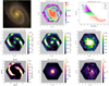 |
Fig. A.1. Analysis maps for the CP galaxy 12067-12705. From left upper to right lower panels: SDSS colour image with the MaNGA FoV, WHAN diagnostic diagram map, WHAN diagnostic diagram scatter plot, Hα emission line map, Hβ emission line map, spectral index Dn4000 map, SFR CIGALE result map, M⋆ CIGALE result map, and χ2 CIGALE result map. |
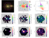 |
Fig. A.2. Analysis maps for the PrM galaxy 8322-12702. From left upper to right lower panels: SDSS colour image with the MaNGA FoV, WHAN diagnostic diagram map, WHAN diagnostic diagram scatter plot, Hα emission line map, Hβ emission line map, spectral index Dn4000 map, SFR CIGALE result map, M⋆ CIGALE result map, and χ2 CIGALE result map. |
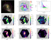 |
Fig. A.3. Analysis maps for the M galaxy 8241-12705. From left upper to right lower panels: SDSS colour image with the MaNGA FoV, WHAN diagnostic diagram map, WHAN diagnostic diagram scatter plot, Hα emission line map, Hβ emission line map, spectral index Dn4000 map, SFR CIGALE result map, M⋆ CIGALE result map, and χ2 CIGALE result map. |
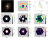 |
Fig. A.4. Analysis maps for the PsM galaxy 9194-3702. From left upper to right lower panels: SDSS colour image with the MaNGA FoV, WHAN diagnostic diagram map, WHAN diagnostic diagram scatter plot, Hα emission line map, Hβ emission line map, spectral index Dn4000 map, SFR CIGALE result map, M⋆ CIGALE result map, and χ2 CIGALE result map. |
Appendix B: Visualisation tools
Marvin, a tool specifically designed to visualise and analyse MaNGA data, has the capability of generating BPT diagrams for a particular galaxy. By default, a spaxel only becomes classified if it meets the criteria in all three diagrams. Even selecting the less strict criterion (based on the [OIII]/Hβ versus [NII]/Hα diagram), it depends on the emission in four lines, where [OIII] and /Hβ might be weak, limiting the area where we could analyse the galaxy. The BPT diagrams also limit the classification of the stellar activity to three categories: the star-formation type (SF), the Seyfert type, and LI(N)ERs type. This last category could also contain some kind of passive activity. It is also possible to create a WHAN diagram for a particular galaxy with Marvin, where the code is provided as a proposed Marvin Science Case Exercise (i.,e., it is not implemented as a functionality). Using only two emission lines (Hα and [NII], which are easily observable in spectra), it is very useful for classifying regions with weak emission-lines that cannot be classified using BPT diagrams. It also identifies weak AGN from fake AGN, named retired galaxies (RGs) from LI(N)ERs, allowing a more complete analysis of regions where the heating of their ionised gas is the result of old stars, rather than star formation or AGN activity.
Taking advantage of the huge potential of the WHAN diagram to investigate galaxy evolution processes at the different stellar population and at galaxy components level, we have developed a tool to visualise the spatially resolved WHAN diagram in MaNGA galaxies10. Based on the WHAN diagnostic diagram, the tool allows us to comprehensively explore the nuclear activity in MaNGA galaxies. Our function is designed to even explore the intermediate areas between adjoining WHAN categories, allowing us to investigate transition processes in the diverse stellar population among different regions of the galaxies. To do this, we use different colours to move gradually from one category to the other, according to their values of WHα and/or [NII]/Hα, translating this information to a map of the galaxy. With this new technique we can study the spatially resolved nuclear activity in MaNGA galaxies, and it can be analysed in more detail than with previous methods. This function allows exploring the AGN/star-formation/quenching activity in the different galaxy components, which may help to investigate, for instance, how the quenching process occurs in galaxies, if there is any relation between Active Galaxy Nuclei (AGN) activity or star-formation with the local environment in close pairs/mergers, whether nuclear activity is concentrate in the inner regions or it is more extended, etc. This function can be easily incorporated in Marvin. In the panels of figures in Appendix A, we show the WHAN diagnostic diagrams and maps for an example galaxy in each merging stage in this work.
The code is 100% based on free software (MIT License), making extensive use of the Python language. We have developed the code under a Linux and Windows platform, and it may be straightforwardly ported to any other operating system (Mac, FreeBSD, etc).
Appendix C: Galaxy morphology and CAS parameters
In this section we compute non-parametric image predictors Gini, M20, and Concentration–Asymmetry–Clumpiness (CAS) parameters (Conselice 2003); 2004AJ....128..163L; 2016MNRAS.456.3032P, which quantitatively determine the morphological characteristics of a galaxy, to compare with the analysis in Hernández-Toledo et al. (2023) and Nevin et al. (2023), who used these parameters to identify merger galaxies, as well as their merging process stage.
In this work, we tested these parameters computed for the galaxies in our sample, in comparison with all MaNGA galaxies, applied to the MaNGA FoV, using the optical wide band maps (r-band) provided by the MaNGA DAP. The correlation between the parameters is shown n Fig. C.1, while the distribution of the parameters for each merger stage is presented in Fig. C.2.
As complement of the Figs. 16 and 17 presented in Sect. 4.2, for reference, we present here as well a version of the SFR-M⋆ diagram where each data point for each galaxy is replaced by its SDSS three-colour image (see Fig. C.3).
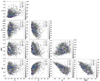 |
Fig. C.1. Comparison between non-parametric image morphological parameters for galaxies in our sample, with different markers and colour-coded as a function of their merger stage according to the legend. Additionally, galaxies presenting lenticular morphology according to DS18 are surrounded by black square. From up-to-down and left-to right: Clumpiness (S), Gini index (G), Moment of light (M20), inverse concentration index (ICI), and asymmetry (A). Background points correspond to the 2D distribution of the same parameters for all MaNGA galaxies, coloured by density of objects. |
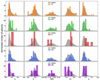 |
Fig. C.2. Distribution of the non-parametric image morphological parameters for galaxies in our sample, with different colour as a function of their merger stage, according to the legend. From left-to right: Clumpiness (S), Gini index (G), Moment of light (M20), inverse concentration index (ICI), and asymmetry (A). The distribution of the same parameters for all MaNGA galaxies is shown (in grey) for reference. |
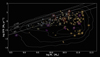 |
Fig. C.3. Integrated SFR − M⋆ diagram for the 137 galaxies in the sample as in Fig. 13, with the point values as the respective SDSS colour image of each galaxy. |
Appendix D: Data catalogue
For the sake of transparency and reproducibility, in Table D.1 we compile the information related to the sample that we have used for the analysis presented in this work.
Physical properties and derived quantities of the galaxies used in this work.
All Tables
All Figures
|
Fig. 1. Projected distance to the nearest companion dnc, in Mpc, with respect to the tidal strength of the central galaxy on the system QA. Contour lines correspond to all the galaxies in the SIP and SIT; green triangles and orange hexagons indicate galaxies in the SIT and SIP, respectively, from MaNGA data. The horizontal solid black line delimits the grey shaded area with dnc ≤ 100 kpc that we use to delimit close pairs. Within this area, the vertical solid black line at QA = − 2 is used to identify interacting galaxies, following Vásquez-Bustos et al. (2023). |
| In the text | |
|
Fig. 2. Post-starburst diagnostic diagram (spectral index distributions Hα equivalent width vs. |
| In the text | |
|
Fig. 3. Spatially resolved PSB diagram (Hα equivalent width vs. |
| In the text | |
|
Fig. 4. MaNGA DAP products used as spectroscopic inputs in CIGALE to estimate physical properties from SED fitting for the galaxy 8241-12705 as example. From left to right: Hα emission line map, Hβ emission line map, and Dn4000 spectral index map. |
| In the text | |
|
Fig. 5. Custom filters over a high and low S/N MaNGA spectra. We show the spectra in two different spaxels for the MaNGA galaxy 12483-12704, one with high S/N (upper panel) and another with low S/N (lower panel) selected from the MaNGA DAP datacube, for comparison. In both panels, the spectra are represented by solid blue lines that cover the full range of the MaNGA spectra, from 3600 to 10 000 Å. The corresponding error is represented by an orange line in the sub-panels. Colour regions show the custom filter wavelength range, with purple, blue, light blue, cyan, green, yellow, orange, and red corresponding to the M3992, M4542, M5446, N6097, N6908, O7473, O8281, and O9265 filters, respectively. The central wavelength that corresponds to each filter is represented by red circles. |
| In the text | |
|
Fig. 6. Signal-to-noise ratio maps for each custom filter for the merger galaxy 8241-12705. From the upper left to lower right, S/N maps for filters M3992, M4542, M5446, N6097, N6908, O7473, O8281, and O9265, respectively. |
| In the text | |
|
Fig. 7. Spatially resolved WHAN diagnostic diagram (upper panel) and map (lower panel) for the merger galaxy 8241-12705. Each colour, and color gradient, corresponds to a WHAN category according to the legend and colourbar, respectively. The WHAN diagram and map were created using the public tool for the visualisation of the spatially resolved WHAN diagnotic diagram for galaxies in the MaNGA survey described in Appendix B. |
| In the text | |
|
Fig. 8. Spatially resolved Σ SFR (left panel), Σ M⋆ (middle panel), and χ2 (right panel) maps from the results of the spectro-photometric SED fitting with CIGALE for the galaxy 8241-12705. The scale of the χ2 map is normalised to the maximum value. |
| In the text | |
|
Fig. 9. Fraction of young and old spaxels for galaxies in each merger stage. We use the Dn(4000) parameter and the divisory value of Dn(4000) = 1.67 (as in Mateus et al. 2006) to separate between young (Dn(4000) ≤ 1.67, in blue) and old (Dn(4000) > 1.67, in orange) spaxels. The number of galaxies in each merger stage is indicated on the right-hand side, with text coloured as in Fig. 10. |
| In the text | |
|
Fig. 10. Mean radial profiles of the Dn(4000) parameter with respect to R/Reff for all the galaxies in each merger stage. The radial profiles are represented in different colours for each merger stage according to the legend. Uncertainties are represented in the same colours at 1σ level. The slope, m, of the linear fit to the mean radial profile up to 1.5R/Reff (marked with a dashed vertical black line), with its corresponding uncertainties, are included in the legend for each merger stage. The number of galaxies in each merger stage is indicated in the lower right-hand corner, with text coloured as denoted in the legend. |
| In the text | |
|
Fig. 11. Percentage of spaxels for each WHAN category for each merger stage. Blue colour bars represent the fractions of PSF spaxels, purple colour bars represent the fractions of sAGN spaxels, green colour bars represent the mean fractions of the wAGN spaxels, orange colour bars represent the fraction of spaxels classified as RG-like emission, and red colour bars represents the fraction of spaxels classified as PG-like emission, according to the WHAN diagnostic diagram. The number of galaxies in each merger stage is indicated in the right side, with text coloured as in Fig. 10. |
| In the text | |
|
Fig. 12. Distribution of the sSFR surface density (ΣsSFR) for spaxels in each WHAN category for each merger stage (the number of galaxies in each category is indicated in parentheses). The distributions are shown in the form of box plots, with a different colour for each WHAN category as in Fig. 11. The median values of the distributions are represented by a horizontal line within the box plots, while the mean values are represented by a white circle. Outlier values (larger than 1.5× the inter-quartile range) are represented by black diamonds. The distribution for passive galaxies is not presented since the values of the ΣsSFR are null. |
| In the text | |
|
Fig. 13. Integrated SFR − M⋆ diagram for the 137 interacting galaxies in our sample. Galaxies classified as CP are represented by orange triangles, galaxies classified as PrM are represented by green hexagonal marks, M galaxies are represented by red stars, and galaxies classified as PsM are represented by blue and purple circles in the case of absence or presence of PSB emission, respectively. In the lower left-hand corner, we present a representative error, given by the mean value of the error of the integrated log SFRmean = 0.223 M⊙ yr−1 and the integrated log M⋆ mean = 0.097 M⊙. As reference, the contour backgrounds correspond to the integrated properties for all MaNGA galaxies from the Pipe3D value-added catalogue (Sánchez et al. 2016a,b), and the grey continuous line correspond to the ‘nurture’ free main sequence for star-forming galaxies derived by Argudo-Fernández et al. (2025). The dashed lines mark the locations with three, four, and seven times above the main sequence (along the SFR axis), respectively. |
| In the text | |
|
Fig. 14. Same as Fig. 13, integrated sSFR − M⋆ diagram for the 137 interacting galaxies in our sample. Galaxies classified as CP are represented by orange triangles, galaxies classified as PrM are represented by green hexagonal marks, M galaxies are represented by red stars, and galaxies classified as PsM are represented by blue and purple circles in the case of absence or presence of PSB emission, respectively. In the lower right-hand corner we present a representative error, given by the mean value of the error of the integrated log SFRmean = 0.24 M⊙ yr−1 and the integrated log M⋆ mean = 0.097 M⊙. As reference, the contours lines correspond to the integrated properties for all MaNGA galaxies from the Pipe3D value-added catalogue (Sánchez et al. 2016a,b). The grey continuous line corresponds to the ‘nurture’ free main sequence for star-forming galaxies derived by Argudo-Fernández et al. (2025). The dashed lines mark the locations with three, four, and seven times above the main sequence (along the SFR axis), respectively. The red continuous line corresponds to the fit to separate star forming from quenched galaxies in the Pipe3D sample, with its corresponding 1σ to delimit the green valley (dashed red lines). |
| In the text | |
|
Fig. 15. Distribution of the integrated sSFR in the form of violin plots for each merger stage. The coloured area determines the density distribution for CP in orange, PrM in green, M in red, PsM in blue, and PSB in purple. For reference, the values of the integrated properties for all MaNGA galaxies (10010 galaxies) from the Pipe3D value-added catalogue (Sánchez et al. 2016a,b) have been added (in grey). The inner box on each violin plot is a representation of the interquartile range of the median (red dot) and its 95% of its confidence intervals. We also show the outlying points of the distributions (if any) as black open circles, which represent the atypical values for that category. The number of galaxies above and below the MS in Fig. 14 is indicated above and below the violin plots, respectively, while the total number of galaxies considered in each merger stage is presented in Table 1. |
| In the text | |
|
Fig. 16. Integrated SFR − M⋆ diagram for the 137 galaxies in the sample as in Fig. 13, with the point values as WHAN maps respectively for each galaxy. The colourbar represents the WHAN categories based on Cid Fernandes et al. (2011). The coloured hexagons indicate the merger stage for each galaxy in the diagram following the colour scheme in Fig. 13. The dashed lines mark the locations with three, four, and seven times above the main sequence (along the SFR axis), and 1/3, 1/4, and 1/7 times below the main sequence, respectively. |
| In the text | |
|
Fig. 17. Integrated SFR − M⋆ diagram for the 137 galaxies in the sample as in Fig. 16, but using maps of the age of the stellar populations instead of WHAN maps. The maps are divided into young blue degraded colour (for spaxels with Dn(4000) ≤ 1.67) and old orange degraded colour (for spaxels with Dn(4000) > 1.67) according to their Dn4000 parameter, respectively for each galaxy. |
| In the text | |
|
Fig. A.1. Analysis maps for the CP galaxy 12067-12705. From left upper to right lower panels: SDSS colour image with the MaNGA FoV, WHAN diagnostic diagram map, WHAN diagnostic diagram scatter plot, Hα emission line map, Hβ emission line map, spectral index Dn4000 map, SFR CIGALE result map, M⋆ CIGALE result map, and χ2 CIGALE result map. |
| In the text | |
|
Fig. A.2. Analysis maps for the PrM galaxy 8322-12702. From left upper to right lower panels: SDSS colour image with the MaNGA FoV, WHAN diagnostic diagram map, WHAN diagnostic diagram scatter plot, Hα emission line map, Hβ emission line map, spectral index Dn4000 map, SFR CIGALE result map, M⋆ CIGALE result map, and χ2 CIGALE result map. |
| In the text | |
|
Fig. A.3. Analysis maps for the M galaxy 8241-12705. From left upper to right lower panels: SDSS colour image with the MaNGA FoV, WHAN diagnostic diagram map, WHAN diagnostic diagram scatter plot, Hα emission line map, Hβ emission line map, spectral index Dn4000 map, SFR CIGALE result map, M⋆ CIGALE result map, and χ2 CIGALE result map. |
| In the text | |
|
Fig. A.4. Analysis maps for the PsM galaxy 9194-3702. From left upper to right lower panels: SDSS colour image with the MaNGA FoV, WHAN diagnostic diagram map, WHAN diagnostic diagram scatter plot, Hα emission line map, Hβ emission line map, spectral index Dn4000 map, SFR CIGALE result map, M⋆ CIGALE result map, and χ2 CIGALE result map. |
| In the text | |
|
Fig. C.1. Comparison between non-parametric image morphological parameters for galaxies in our sample, with different markers and colour-coded as a function of their merger stage according to the legend. Additionally, galaxies presenting lenticular morphology according to DS18 are surrounded by black square. From up-to-down and left-to right: Clumpiness (S), Gini index (G), Moment of light (M20), inverse concentration index (ICI), and asymmetry (A). Background points correspond to the 2D distribution of the same parameters for all MaNGA galaxies, coloured by density of objects. |
| In the text | |
|
Fig. C.2. Distribution of the non-parametric image morphological parameters for galaxies in our sample, with different colour as a function of their merger stage, according to the legend. From left-to right: Clumpiness (S), Gini index (G), Moment of light (M20), inverse concentration index (ICI), and asymmetry (A). The distribution of the same parameters for all MaNGA galaxies is shown (in grey) for reference. |
| In the text | |
|
Fig. C.3. Integrated SFR − M⋆ diagram for the 137 galaxies in the sample as in Fig. 13, with the point values as the respective SDSS colour image of each galaxy. |
| In the text | |
Current usage metrics show cumulative count of Article Views (full-text article views including HTML views, PDF and ePub downloads, according to the available data) and Abstracts Views on Vision4Press platform.
Data correspond to usage on the plateform after 2015. The current usage metrics is available 48-96 hours after online publication and is updated daily on week days.
Initial download of the metrics may take a while.