| Issue |
A&A
Volume 696, April 2025
|
|
|---|---|---|
| Article Number | A178 | |
| Number of page(s) | 15 | |
| Section | Interstellar and circumstellar matter | |
| DOI | https://doi.org/10.1051/0004-6361/202450965 | |
| Published online | 25 April 2025 | |
The impact of expanding HII regions on filament G37
Curved magnetic field and multiple direction material flows
1 School of Astronomy and Space Science, Nanjing University, 163 Xianlin Avenue, Nanjing 210023, PR China
2 Xinjiang Astronomical Observatory, Chinese Academy of Sciences, Urumqi 830011, PR China
3 University of Chinese Academy of Sciences, Beijing 100049, PR China
4 Key Laboratory of Radio Astronomy and Technology (Chinese Academy of Sciences), A20 Datun Road, Chaoyang District, Beijing 100101, PR China
5 Xinjiang Key Laboratory of Radio Astrophysics, Urumqi 830011, PR China
6 Key Laboratory of Modern Astronomy and Astrophysics (Nanjing University), Ministry of Education, Nanjing 210023, Jiangsu, PR China
★ Corresponding authors: This email address is being protected from spambots. You need JavaScript enabled to view it.
; This email address is being protected from spambots. You need JavaScript enabled to view it.
Received:
3
June
2024
Accepted:
28
February
2025
Abstract
Filament G37 exhibits a distinctive “caterpillar” shape, characterized by two semicircular structures within its 40 pc-long body, and provides an ideal target to investigate the formation and evolution of filaments. By analyzing multiple observational data, such as the CO spectral line, the Hα radio recombination line, and the multiwavelength continuum, we find that the expanding H II regions that surround filament G37 exert pressure on the structure of the filament body, which kinetic process present as the gas flows in multiple directions along the skeleton of the filament body. The curved magnetic field structure of filament G37 derived by employing the velocity gradient technique with CO is found to be parallel to the filament body and support the pressure from expanded H II regions. The multidirectional flows in filament G37 could cause the accumulation and subsequent collapse of gas, which would result in the formation of massive clumps. The curved structure and star formation observed in filament G37 are likely to be a result of the filament body being squeezed by the expanding H II region. This physical process occurs over a timescale of approximately 5 Myr. Filament G37 provides a potential candidate for end-dominated collapse.
Key words: stars: formation / ISM: clouds / evolution / HII regions / ISM: magnetic fields
© The Authors 2025
 Open Access article, published by EDP Sciences, under the terms of the Creative Commons Attribution License (https://creativecommons.org/licenses/by/4.0), which permits unrestricted use, distribution, and reproduction in any medium, provided the original work is properly cited.
This article is published in open access under the Subscribe to Open model. This email address is being protected from spambots. You need JavaScript enabled to view it. to support open access publication.
1 Introduction
In the Milky Way, giant molecular clouds represent the coldest and densest regions (Field et al. 1969; McKee & Ostriker 1977). These regions exhibit intricate filamentary structures that span a wide range of environments within the interstellar medium (ISM) (e.g., Schneider & Elmegreen 1979; Bally et al. 1987; Williams et al. 2000; Kauffmann et al. 2008; Men’shchikov et al. 2010; Zucker et al. 2018). These filamentary structures are believed to play a crucial role in the process of star formation (André et al. 2014). Notably, the analysis of Herschel data has revealed a strong correlation between filamentary clouds and the occurrence of star formation (André et al. 2010, 2014; Wang et al. 2015; Stutz 2018). Specifically, filament structures of various sizes within the ISM have been closely associated with star formation (e.g., Schneider & Elmegreen 1979; Bally et al. 1987; Hacar et al. 2013; Li et al. 2013; Anderson et al. 2014; Hacar et al. 2017; Dewangan et al. 2019; Yuan et al. 2020; Bhadari et al. 2020, 2022). Therefore, comprehending the physical origins and evolutionary processes of these filaments is crucial for a comprehensive understanding of star formation as a whole (Hacar et al. 2023).
The formation and evolution of filaments within the ISM pose significant unresolved questions (e.g., Li et al. 2013, 2016; Zucker et al. 2018; Hacar et al. 2023). Understanding the kinematics of the ISM, including gas velocity information, is crucial for elucidating the radial velocities of gas filaments and their relationship to star formation processes (Stutz & Gould 2016; Hacar et al. 2018). By examining gas radial velocities, valuable insights can be gained into the physical properties and internal dynamics of observed filaments (Hacar & Tafalla 2011; Zernickel et al. 2013; Hacar et al. 2017, 2018; Lu et al. 2018). The kinematics of gas play a pivotal role in unraveling the underlying physical mechanisms involved in filament formation and the conversion of gas mass into stellar mass within filaments (e.g., Li et al. 2014; Liu et al. 2019; Yuan et al. 2020; He et al. 2023; Ma et al. 2023). Filaments in the Milky Way with many different morphologies (Wang et al. 2015, 2016) is a not clearly understood problem. The shape of the molecular clouds could be caused by their being squeezed by nearby HII region (Li et al. 2013; Wolfire et al. 2022; Zucker et al. 2022). Furthermore, the impact of star formation activities in the ISM is noteworthy (e.g., Zhang et al. 2016; Arzoumanian et al. 2021; Arzoumanian et al. 2022). These activities, such as outflow, radiation, shocks, and stellar wind, are common phenomena that impact and reshape the structure of the ISM (e.g., Churchwell et al. 2006, 2007; Hou & Gao 2014). Additionally, magnetic field plays an important role in star formation and filament evolution but the details of this process are not clearly understood (e.g., Crutcher 2012; Hull & Zhang 2019; Arzoumanian et al. 2021; Doi et al. 2021; Li 2021; Ching et al. 2022; Hwang et al. 2022; Kwon et al. 2022; Wang et al. 2024; Zhao et al. 2024a). Regions of active star formation exhibit similarities in the morphology of their gas and magnetic fields (Pattle et al. 2017; Doi et al. 2020; Arzoumanian et al. 2021).
Filament G037.410-0.070 (hereafter, G37), located at l = 37.4° and b = –0.03°, exhibits a distinctive spectral shape resembling a “caterpillar” when observed at submillimeter and far-infrared wavelengths (Li et al. 2016; Rigby et al. 2016; Zucker & Chen 2018). In near- and mid-infrared images, three bright objects can be identified within the filament body (Wang et al. 2016). This filament was identified by Li et al. (2016), Rigby et al. (2016), Wang et al. (2016), and Zucker & Chen (2018), and presents an ideal target to investigate the impact of dynamics, H II region expansion, and magnetic fields on filament and star formation. Extensive data from various surveys have covered this region, including CO observations (Jackson et al. 2006; Dempsey et al. 2013; Reid et al. 2016; Rigby et al. 2016; Umemoto et al. 2017), infrared continuum measurements (Benjamin et al. 2003; Carey et al. 2009; Men’shchikov et al. 2010; Poglitsch et al. 2010; Griffin et al. 2010), and centimeter wavelength observations (Stil et al. 2006). The unique morphology of filament G37 provides a valuable sample for studying filament formation and evolution.
In this study, our objective is to investigate the dynamics and magnetic field properties of filament G37, as well as explore the potential mechanisms involved in filament formation. The paper is structured as follows. The archival data used in this study are detailed in Sect. 2. The basic physical, dynamics, and magnetic field properties of filament G37 are presented in Sect. 3. The potential formation mechanisms of filament G37 are explored in Sect. 4. A summary of the findings is provided in Sect. 5.
2 Archival data
2.1 Spectroscopic data
Carbon monoxide (CO) serves as an excellent tracer for studying the kinematic properties of molecular clouds. The spectroscopic data utilized in this study is derived from the CO High-Resolution Survey (COHRS), specifically the 12CO (J = 3–2) transition, which was observed by the James Clerk Maxwell Telescope (JCMT) (Dempsey et al. 2013). The survey covers a region with |b| ≤ 0.5° and 10.25° ≲ l ≲ 56°. The beam size of the observations is ~15ʺ with a velocity resolution of 1 km s−1 and a pixel size of about 6ʺ. The average root mean square (RMS) noise level is ~1 K. Additionally, this study incorporates the 13CO and C18O (J = 3–2) emissions from the 13CO/C18O (J = 3– 2) Heterodyne Inner Milky Way Plane Survey (CHIMPS), which was carried out. The CHIMPS survey covers a region with |b| ≤ 0.5° and 28° ≲ l ≲ 46°. The spatial resolution for the 13CO and C18O emissions is 14ʺ with a velocity resolution of 0.5 km s−1 and a pixel scale of 7ʺ. The median RMS noise level is ~0.6 K.
The ionized gas is effectively traced by the Hα radio recombination line (RRL). For this investigation, we utilized the Hα RRL data obtained from the Green Bank Telescope (GBT) Diffuse Ionized Gas Survey (GDIGS; Anderson et al. 2021). The Hα RRL emission was quantified through the measurement of the 4–8 GHz. The beam size employed was 2.8ʹ with a velocity resolution of 0.5 km s−1.
2.2 Continuum data
In this work, continuum data is used at different wavelengths. The 850 μm continuum emission is observed by the JCMT telescope (JCMT Plane Survey, Eden et al. 2017), whose resolution is around 14ʺ. The continuum at the mid-infrared wavelength is observed by Spitzer at 3.6, 8, and 24 μm (Spitzer, GLIMPSE Benjamin et al. 2003; MIPSGAL Carey et al. 2009) with resolutions of 1.2ʺ, 2ʺ, and 6ʺ, respectively. The continuum at 1420 MHz is observed by the Very Large Array (VLA) from the VLA Galactic Plane Survey (VGPS) (Stil et al. 2006), whose resolution is around 44ʺ.
2.3 Column density and dust temperature
The H2 column density and dust temperature maps1 of filament G37 come from Zucker et al. (2018), and were derived via a spectral energy distribution (SED) fitting procedure (Wang et al. 2015) on the Herschel continuum at wavelengths of 70, 160, 250, 350, and 500 μm.
2.4 Polarization data
The 353 GHz dust polarized emission, obtained from the Planck satellite2 (Planck Collaboration XII 2020; Planck Collaboration XI 2020), offers a valuable means to investigate the large-scale magnetic field structure of molecular clouds, as demonstrated in previous studies (Planck Collaboration Int. XXXV 2016). Utilizing observations from the High-Frequency Instrument (HFI; Planck Collaboration III 2020), researchers have generated maps of the Stokes parameters I, Q, and U, along with their corresponding dispersion values (σI, σQ, σU). These maps have a resolution of 5ʹ and a pixel size of ~1.7ʹ. The polarization angle can be derived from the HFI Stokes maps, ψPlanck = 0.5 × arctan(U, Q), where ψPlanck varies from –90° to 90° with the HEALPix convention. To align with the IAU convention, the Planck measurement needs to be converted using the equation ψ = 0.5 × arctan(–U,Q). To ascertain the orientation of the magnetic field (referred to as the B-field), one can obtain ψB by adding 90° to the polarization angle. This can be achieved using the equation ψB = ψPlanck + 90°.
3 Results
3.1 Overview
Previous studies conducted by Li et al. (2016), Wang et al. (2016), Rigby et al. (2016), and Zucker et al. (2018) have identified and characterized filament G37, and revealed a velocity range of 51 to 63 km s−1. Utilizing the Bar and Spiral Structure Legacy (BeSSeL) Survey calculator (Reid et al. 2019), there are around a 50 percent probability that the filament G37 is situated in the Sagittarius far arm, approximately 9.3±0.5 kpc away. The length of filament G37 measures ~41±2 pc.
As depicted in Fig. 1, the 850 μm emission of filament G37 reveals a distinct shape reminiscent of a caterpillar, featuring two semicircular structures within its main body. Zucker et al. (2018) have identified four dense clumps along the skeleton of filament G37. These clumps, namely C1, C2, C3, and C4, correspond to the eastern endpoint of filament G37, the peak position of the larger semicircular structure, the junction point between the two semicircular structures, and the western end-point of filament G37, respectively. These clumps exhibit higher brightness in the 850 μm emission compared to other regions of the filament. Additionally, Fig. 1 displays bright emissions at 3.6, 8, and 24 μm in these clumps, indicative of ongoing star formation activities resulting from the heating of dust by newly formed stars. Therefore, these clumps are likely sites of active star formation.
Surrounding filament G37, emissions at 8 μm occur within two semicircular structures, as depicted in Fig. 1. Additionally, the 1420 MHz and Hα RRL emissions were observed in the same region. These emissions suggest the existence of H II regions in the vicinity of filament G37.
Based on the Spicy Survey (Kuhn et al. 2021) and Gaia Early Data Release 3 (EDR3) (Bailer-Jones et al. 2021) catalog, we found multiple young stellar object (YSO) candidates associated with filament G37 and H II regions. We selected the YSOs from the Spicy Survey catalog that are located at distances greater than 5 kpc, utilizing the Gaia database. This selection criterion is based on the filament’s distance, which is approximately 9.3 kpc. Notably, some YSO candidates are found within the filament body itself and near the four dense clumps, as illustrated in Fig. 1. These findings suggest the potential for star formation within filament G37.
Figure 1 illustrates the spatial distribution of H2 column density (N(H2)) and dust temperature (Tdust) within filament G37, as determined through SED fitting of far-infrared continuum observations obtained by the Herschel telescope at wavelengths of 70, 160, 250, 350, and 500 μm (Zucker et al. 2018). The column density of filament G37 ranges from 1.0 × 10²² to 2.3 × 1022 cm−2, with a mean value of ~1.3 × 1022 cm−2 (see also Table 1). Notably, the column density structure aligns well with the distribution of 850 μm emissions (see Fig. 1). The four dense clumps (C1, C2, C3, and C4) exhibit high column density values of ~1.3–1.8 1022 cm−2.
Regarding the dust temperature, filament G37 displays a range of 15 to 24 K. The dense clumps C1, C2, C3, and C4 exhibit slightly lower dust temperatures, averaging around 20 K. Conversely, the regions within the two semicircular structures generally exhibit higher dust temperatures, ranging from 24 to 35 K. This temperature contrast between the interior and exterior of filament G37 is significant.
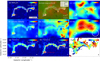 |
Fig. 1 Structure of filament G37. Panels a, b, and c display the structure of filament G37 at different wavelengths. Panel a presents the submillimeter wavelength emission at 850 μm (Eden et al. 2017). The orange line displays the skeleton of filament G37, which is identified in Li et al. (2016). Four special dense clumps (C1–C4) are denoted by red crosses (see Sect. 3.1). The RGB image at the mid-infrared (Spitzer, GLIMPSE Benjamin et al. 2003; MIPSGAL Carey et al. 2009) is shown in panel b, where red represents 24 μm, green represents 8 μm, and blue represents 3.6 μm. Panel c displays the distribution of continuum emission at 1420 MHz from VGPS (Stil et al. 2006). The cross markers in panels b and c display the position of the young stellar objects (YSOs; Kuhn et al. 2021), which are derived from the mid-infrared range of 3–9 μm obtained from the Spitzer telescope. Panels d and e display the distribution of H2 column density and dust temperature (Zucker et al. 2018). The integrated intensity maps of Hα RRL, 12CO (3–2), and 13CO (3–2) emissions from a velocity of 51 to 62 km s−1 are shown in the panels f, g, and h, respectively. The white contours in all panels show the integrated intensity of 13CO (3–2) from 3 to 15 K km−1 with steps of 3 K km−1. The distribution of excitation temperature derived from 12CO (3–2) emission is shown in panel (i). The spatial resolution of each panel is shown in the lower-right corner. |
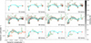 |
Fig. 2 Channel maps of 12CO and 13CO (3–2) emissions for filament G37. The intensity of the 12CO and 13CO (3–2) lines within the velocity range of 51 to 62 km s−1 is depicted by green and red contours, respectively, with a step of 1 km s−1. These contours represent regions where the signal-to-noise ratios of 12CO and 13CO exceed 6σ of the spectral lines, which correspond to approximately 1.9 and 2.1 K km s−1, respectively. The intensity distribution of 12CO emission for each velocity channel is displayed as the gray background of the maps. The skeleton of filament G37 is represented by a cyan line, while four special dense clumps (C1–C4) are denoted by red crosses, which are consistent with those shown in Fig. 1. |
Physical parameters of filament G37.
3.2 Distributions of CO and Hα radio recombination line
In this study, we employ the 12CO, 13CO, C18O, and Hα RRL emissions to investigate the dynamical properties of filament G37. Three mean spectral lines of 12CO, 13CO, and Hα RRL observed in filament G37 are illustrated in Fig. A.1. The identification of filament G37 and determination of its velocity range as 51–63 km s−1 were accomplished by Zucker et al. (2018). To visualize the gas morphology within the filament, intensity maps of the 12CO, 13CO, and Hα RRL emissions at velocity of 51–63 km s−1 are presented in Fig. 1.
In the central region of the body of filament G37, a notable agreement is observed between the dust emission at 850 μm and the emissions of 12CO and 13CO within the primary section of the filament, as depicted in Fig. 1. However, a discrepancy arises between the 850 μm and 12CO, 13CO emissions towards the southern portion of a small semicircular structure associated with filament G37. Specifically, a clump (VLSR(CO) = ~42 km s−1) is detected in the 850 μm continuum, but it does not correspond to the intensity map of the 12CO and 13CO emissions at a velocity range of 51–63 km s−1. This discrepancy suggests that the clump and filament G37 may not occupy the same position along the line-of-sight (LOS) direction.
The distribution of diffuse gas, as traced by the 12CO (3– 2), is observed in the northeastern and northwestern regions of filament G37 (see Figs. 1 and 2). Notably, the highest integrated intensity values from both 12CO and 13CO emissions are found at the extremities of filament G37. Furthermore, within this region, two dense clumps are identified. The first clump, G37.341-00.062, is associated with young star objects identified through the APEX Telescope Large Area Survey of the Galaxy (ATLASGAL) survey (Urquhart et al. 2014), as depicted in Fig. 1. The second clump corresponds to the H II region G37.469-0.104, as cataloged in the Wide-Field Infrared Survey Explorer (WISE) catalog (Anderson et al. 2014), also shown in Fig. 1.
The Hα RRL emissions exhibit similarities to the 1420 MHz emission (see Fig. 1). The occurrence of multiple Hα RRL emissions surrounding the two semicircles of filament G37 indicates the presence of H II regions in close proximity to the filament. In the H II region denoted as G37.469-0.104 (Anderson et al. 2014), weak emissions of Hα RRL and 1420 MHz continuum are observed. This implies that G37.469-0.104 is potentially a compact H II region.
An estimation of the excitation temperature for 12CO (3–2) can be achieved through the application of local thermodynamic equilibrium (LTE) as described by Paron et al. (2014),
![Mathematical equation: $T_{\rm ex}(^{12}{\rm CO}\,3-2)\,=\,\frac{16.59}{{\rm ln}[1+16.59/\,(T_{\rm mb}+0.036)]} ~~{\rm K},](/articles/aa/full_html/2025/04/aa50965-24/aa50965-24-eq1.png) (1)
where Tmb is the peak temperature of 12CO (3–2) emission. Figure 1 illustrates a complex distribution of excitation temperatures within filament G37. We observe that the excitation temperature of the predominant gas within the filament ranges from 25 to 41 K. The excitation temperature is not uniformly distributed along the filament body. Notably, clumps C2 and C4 exhibit elevated temperatures that exceed 30 K (see Fig. 1). Additionally, outside the semicircular structure, the area adjacent to clump C2 also displays a high excitation temperature. In contrast, the excitation temperatures of other regions along the filament are comparable to the dust temperature.
(1)
where Tmb is the peak temperature of 12CO (3–2) emission. Figure 1 illustrates a complex distribution of excitation temperatures within filament G37. We observe that the excitation temperature of the predominant gas within the filament ranges from 25 to 41 K. The excitation temperature is not uniformly distributed along the filament body. Notably, clumps C2 and C4 exhibit elevated temperatures that exceed 30 K (see Fig. 1). Additionally, outside the semicircular structure, the area adjacent to clump C2 also displays a high excitation temperature. In contrast, the excitation temperatures of other regions along the filament are comparable to the dust temperature.
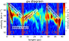 |
Fig. 3 Position-velocity (P-V) diagram to illustrate the distribution of filament G37, obtained from 13CO emission. The distribution is shown along the filament skeleton, as depicted in Fig. 2, with the dense clumps C1, C2, C3, and C4 (as shown in Fig. 1) represented by the red columns. The x-axis denotes the filament length in unit as pc, while the y-axis shows the velocity, VLSR. The diagram shows vertical dashed red lines for the locations of four dense clumps (C1–C4) and black lines for the velocity gradients. The extra velocity gradient of clump C1 is shown as a dashed line. |
3.3 Velocity field
Figure 2 illustrates the channel maps of 12CO and 13CO (3– 2) of filament G37, which span from VLSR = 51 to 62 km s−1. The gas structures observed in the 12CO and 13CO (3–2) emissions exhibit similar characteristics in each velocity channel. The molecular tracer 12CO reveals more detailed structures within the diffuse molecular gas compared to the 13CO emission. Initially, at velocities of 51 to 54 km s−1, the dense clump C4 (G37.341-00.062) emerges, followed by the eastern top of the large semicircle (Clump C2) and the connecting part between the two semicircles (Clump C3). The molecular gas exhibits an east-to-west flow along the filament structure within the small semicircle, towards the dense clump C4. Between VLSR = 53 and 55 km s−1, the gas within the two semicircular structures of the filaments gradually converges toward the connecting part (Clump C3). The gas within the large semicircle flows from the top part (Clump C2) toward the two sides (Clumps C1 and C3). Subsequently, from VLSR = 54 to 59 km s−1, the gas flows from west to east, following the filament structure. From VLSR = 59 to 62 km s−1, only Clump C1 remains, and gradually diminishes.
The position-velocity (P-V) diagram depicted in Fig. 3 corresponds to the filament skeleton, as illustrated in Fig. 1. Material flows predominantly occur within the filament, as evidenced by the channel maps and P-V diagram presented in Figs. 2 and 3, respectively. Notably, significant velocity gradients are observed between the dense clumps C1 and C2, as well as between C3 and C4, at approximately 0.46 and 0.49 km s−1 pc−1, respectively. Between the dense clumps C2 and C3, the left portion of the filament exhibits a distinct velocity gradient of ~0.4 km s−1 pc−1, while the velocity distribution in the other half remains unclear. In the vicinity of the dense clump C1 within a radius of less than 5 pc, a significant velocity gradient is detected, as illustrated in Fig. 3, which exhibits a wide range of velocities (~2.4 km pc−1, see Fig. 2). A similar result has been found in the OMC-1 region, where a velocity gradient of 5–7 km pc−1 was measured (Hacar et al. 2017). This phenomenon may indicate the presence of accelerated motions towards the massive dense clump C1.
Figure B.1 illustrates the distribution of the central velocity (VLSR) along the LOS and the velocity dispersion (σV) for both 12CO and 13CO (3–2) emissions. The coverage region of the central velocity and velocity dispersion maps derived from 13CO (3–2) is limited to areas where the signal-to-noise ratios (S/N) exceed 2σ (5 K km s−1). In comparison to the 13CO, the S/Ns of the 12CO emission are relatively high. In Fig. B.1, the coverage region of 12CO exceeds 5σ (5.5 K km s−1). As depicted in Fig. B.1, the velocity distribution within the western region of the filament is relatively low, while it is higher in the eastern region. Furthermore, the velocity dispersion of 13CO is lower compared to that of 12CO. The diffuse gas that surrounds the filament displays a higher velocity dispersion, as measured by the 12CO spectral line.
3.4 Magnetic field
As mentioned in Sect. 3.1, filament G37 is situated in the Sagittarius far arms, ~9.2 kpc away, within the Galactic plane. The measurement of the magnetic field of filament G37 poses a challenge due to foreground and/or background effects, as it traverses multiple spiral arms along the LOS. A new technique, the velocity gradient technique (VGT), can probe the magnetohydrodynamic (MHD) turbulent anisotropy from a position-position-velocity cube to infer the magnetic field (Hu et al. 2019; Zhao et al. 2022, 2024b,c). Therefore, we employ the VGT (González-Casanova & Lazarian 2017; Lazarian & Yuen 2018; Hu et al. 2018; Zhao et al. 2024b,c) to measure the magnetic field, which mitigates the influence of foreground and/or background effects. The description and accuracy of the VGT are elaborated in Appendix C. The application of VGT analysis to all velocity components can validate the accuracy of VGT in relation to the magnetic field within this region (see Fig. C.1). By utilizing the velocity component of filament G37, we can delineate the magnetic field structure of G37 clearly, free from the influence of foreground and background effects (see Appendix C).
The velocity dispersion at each pixel exceeds 1 km s−1 (velocity channel width), which indicates that the velocity channels derived from the position-position-velocity (PPV) cube of 12CO and 13CO (3–2) emissions are narrow (Lazarian & Yuen 2018). This narrow velocity channel can effectively trace the turbulent velocity field (Lazarian et al. 2001). The spectral lines of 12CO exhibit a high S/N, which enables the differentiation of various velocity components within the G37 filament region (see Fig. C.1). In contrast, the S/N of 13CO is insufficient to validate the accuracy of the VGT for tracing the magnetic field (see Fig. A.1). To measure the magnetic field of filament G37, we applied the VGT to the 12CO spectral line at a velocity range of 51–64 km s−1 (see Sect. 3.1), which corresponds to velocity component 4 of filament G37, as shown in Fig. C.1. The magnetic field structure of filament G37 is presented in Fig. 4. The magnetic field resolution is 2ʹ, and the sub-block size was set to 20×20 pixels. In all cases, the magnetic field structure was found to be nearly parallel to filament G37 (see Fig. 4). Within the large semicircle of filament G37, the magnetic field orientations were distributed along the filament and aligned parallel to its elongation direction. Conversely, within the small semicircle, the magnetic field orientations were parallel to the Galactic plane and aligned in the east-west direction.
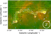 |
Fig. 4 Magnetic field structure of filament G37 revealed with VGT measurements of 12CO. The orientation of the magnetic field is represented as black vectors. The intensity map of filament G37, derived from 13CO emission, is depicted as white contours (same as Fig. 1). The background of the image corresponds to a mid-infrared three-color map, consistent with Fig. 1. The spatial resolution of the magnetic field measurement using VGT is ~2ʹ, as indicated by a white circle in the bottom-right corner. |
3.5 Identification of clumps
Multivelocity components exist around the filament along the LOS orientation (see Figs. A.1, C.1, and Sect. 3.4). The velocity-integrated intensity maps of these components are presented in Fig. D.1. The H2 column density obtained from Herschel (Zucker et al. 2018) exhibits a structure similar to that of component 4, which corresponds to a velocity range of 51–63 km s−1 and delineates filament G37. In contrast, the other components display weak 12CO emissions and diffuse distributions that partially overlap with filament G37. Consequently, the emissions observed from Herschel and the 850 μm continuum are likely to be primarily associated with filament G37. To identify the location of clumps in filament G37, we employed 13CO (3–2) and 850 μm emissions. The clumps found in the 850 μm emission that corresponded to the velocity range 51–62 km s−1 of 13CO emission were considered to be situated on filament G37. We identified 17 dense clumps that are located within filament G37 (details see Appendix E). The positions of clumps are shown in Fig. E.1 and Table E.1. We assume that each clump is a uniform sphere (Fiege & Pudritz 2000). The effective radii, R, of clumps can be estimated by  , where the A is the coverage area of clumps. The clump size is the effective diameter (D = 2R). The mass of clumps, M, is calculated by M = N(H2) μmHA, where N(H2) is the H2 column density, μ is the mean molecular weight for clouds as 2.37, mH is the mass of a H atom. The details of the parameters of dense clumps are shown in Table E.1.
The timescale that reflects the evolutionary features of a filament is the time it takes to grow to reach its critical line mass (Mcri). This timescale is known as the critical timescale (τcri) and represents the lower age limit of the filament. The function of the fragmentation length scale can be used to calculate the critical timescale, τcri (Williams et al. 2018),  , where λcore represents the separation between the clumps/cores in a filament. The length between nearby clumps in filament G37, λcore, is roughly estimated at around 3 pc due to the low spatial resolution. The critical timescale (τcri) for filament G37 is estimated to be approximately 4.9 Myr. However, this estimation is subject to considerable uncertainties that arise from several factors, including limited spatial resolution, distance measurement errors, and projection effects. Notably, the separation between clumps (λcore) within G37 is highly uncertain. Furthermore, the assumption of uniform temperature variations introduces additional errors into the estimation. As a result, the critical timescale of τcri ~ 4.9 Myr should be regarded as a lower limit for filament G37, accompanied by a degree of uncertainty.
4 Discussion
4.1 Material flows and end collapse
Filament G37 is a unique sample that distinguishes itself from other giant filaments located in the Galactic plane. What sets it apart is not only its curved configuration but also its presence within multi-directional material flows. While the curvature of filaments in the Galactic plane is not uncommon, such as is seen in G51, G11, G47, IC 446/IC 447, and NGC 6334 (Li et al. 2013; Zernickel et al. 2013; Wang et al. 2015; Bhadari et al. 2020), filament G37 diverges in its characteristics. Unlike the velocity structure of these giant filaments (Zhao et al. 2024b), multiple velocity gradients (around 0.5 km s−1 pc−1) are found in filament G37 (see Fig. 3), in which the material flows from the top of the large semicircle to the end of this structure, while there is another flow from the connecting point of the two semicircle structures to the end of the filament body. The material flows along the two semicircular structures of filament G37 and exhibits velocity gradients in multiple directions (details see Sect. 3.3). The obvious multidirectional material flows occur at the top point of the large semicircular structure where the flow direction of the material changes (see Fig. 3). This phenomenon was also observed in filament S242 (Dewangan et al. 2019; Yuan et al. 2020).
The gravitational instability of filaments can be determined by the critical line mass, Mcri, which is reached when the line mass is above the critical value. The critical line mass can be estimated using the kinetic temperature (Tk) (Ostriker 1964):
 (2)
where cs is sound speed. The dust temperature, Td, is adopted as the kinetic temperature, Tk, of gas in this work. The critical mass, Mcri, of filament G37 is estimated to be between 30–43 M⊕ pc−1. The total mass of filament G37 is measured to be around 70– 135 M⊕ pc−1, which is much higher than the critical mass. This suggests that filament G37 is undergoing gravitational instability. The filament body may break apart, forming clumps. The initial aspect ratio, A, of a filament is defined as A = L/2R, where L is the filament length and R is the effective radius of the filament. If A is less than 5, homologous collapse is observed, whereas if A is greater than 5, terminal-dominated collapse is predominant (Pon et al. 2011, 2012). The initial aspect ratio, A, of filament G37 is ~6.7. End collapse is most likely to occur in filament G37, where H II regions G37.469-0.104 and dense clump G37.341-0.062 have formed at the end of the filament body. Filament G37 provides a potential candidate for end-dominated collapse.
(2)
where cs is sound speed. The dust temperature, Td, is adopted as the kinetic temperature, Tk, of gas in this work. The critical mass, Mcri, of filament G37 is estimated to be between 30–43 M⊕ pc−1. The total mass of filament G37 is measured to be around 70– 135 M⊕ pc−1, which is much higher than the critical mass. This suggests that filament G37 is undergoing gravitational instability. The filament body may break apart, forming clumps. The initial aspect ratio, A, of a filament is defined as A = L/2R, where L is the filament length and R is the effective radius of the filament. If A is less than 5, homologous collapse is observed, whereas if A is greater than 5, terminal-dominated collapse is predominant (Pon et al. 2011, 2012). The initial aspect ratio, A, of filament G37 is ~6.7. End collapse is most likely to occur in filament G37, where H II regions G37.469-0.104 and dense clump G37.341-0.062 have formed at the end of the filament body. Filament G37 provides a potential candidate for end-dominated collapse.
4.2 Expanding H II region
The morphology of filament G37 exhibits a distinctive feature that consists of two semicircular structures resembling a “caterpillar”, which could be caused by compression from surrounding H II regions. The extended 1420 MHz continuum emission that surrounds filament G37 is the candidate H II region that is affecting the filament body (see Fig. 1). The Hα RRL has a similar peak velocity to that of filament G37 system velocity traced by the 12CO, 13CO spectral lines (see Fig. A.1). The H II regions traced by Hα RRL (see Fig. 1) could be close to filament G37 in three-dimensional space, which could affect the structure and physical processes of filament G37. Compared with the inner part of filament G37, the high dust temperature regions exist near the H II regions (see Fig. 1), which may show that these H II regions are heating the filament body. These H II regions could affect the filament body and cause the formation of the two semicircular structures of filament G37.
The H II regions traced by Hα RRL have noticeable velocity gradients when they cross the filament body (see Fig. 5). These velocity gradients at the top points of the large and small semi-circular structures are estimated to be 1.1 and 0.5 km s−1 pc−1 of blue shift, respectively. In the two semicircular structures, a notable disparity in blue-shifted velocities is observed between the molecular gas, traced by CO, and the ionized gas emanating from the H II regions, probed by Hα RRL (see Fig. 6). The diffuse molecular gas (traced by 12CO) and the dense gas (traced by 13CO and C18O) exhibit a similar blue-shifted velocity difference. These observations serve as direct evidence that the H II region adjacent to filament G37 is expanding towards the blue-shift direction, exerting pressure on the primary body of the filament and contributing to its heating on a large scale. The multidirectional material flows may be influenced by the expansion process that originates from H II regions, with their directional transition point typically situated near the apex of the semicircular structure compressed by the expanding H II region.
The timescale of the formation of the semicircular structures on filament G37, ts, can be roughly estimated using the physical process that is likely to be caused by the squeezing of the filament body by the H II region, ts = l/vs, where l is the squeezing distance and vs is the squeezing velocity of the expanding H II region traced by Hα RRL. The squeezing distance of the large semicircle is around 5 pc (see Fig. 6), which is estimated as extending from clump C2 to the perpendicular distance of the line that connects clump C1 and C3. The squeezing distance of the other small semicircle is around 2.4 pc. The squeezing velocities on the large and small semicircles are equal to the velocity gradient of H II regions as 1.1 and 0.5 km s−1 pc−1, respectively (see Fig. 5). The two semicircular structures could have formed at a similar time and the formation timescale is estimated to be around 5 Myr.
When an H II region expands at the border of filament G37 (see Fig. 1), it can initiate the formation of stars in its vicinity. The H II region creates variations in density and pressure within the surrounding interstellar medium. These variations can cause molecular clouds, which are dense regions of gas, to collapse under their gravity. As the clouds collapse, they fragment into smaller clumps, which eventually form protostars. The high-energy radiation emitted by the H II region can also heat up the surrounding gas, which further promotes the collapse and fragmentation process. Ultimately, this leads to the birth of new stars within the expanding H II region. As stated in Sect. 3.1, filament G37 has been subject to ongoing observations of star formation activities. The fragmentation at the filament body of G37 is similar to the shell fragmentation of the Collect and Collapse (CC) model (Brand et al. 2011). Clumps C1, C3, and C4 represent the nearest structures along the filament to the H II region, which may exhibit an age greater than that of the other clumps and the additional fragmentation observed within the filament (as detailed in Table E.1). This proximity suggests a potential association with sequential star formation, as described in the CC model (Whitworth et al. 1994). It is postulated that the expanding H II region could serve as a significant trigger mechanism for the star formation processes that transpire within filament G37. The phenomena observed in G37 are analogous to the CC model of triggered star formation that occurs in dense shells surrounding H II regions (Whitworth et al. 1994; Deharveng et al. 2008; Brand et al. 2011).
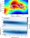 |
Fig. 5 Position–velocity diagram obtained from Hα RRL observations. In the top panel, the intensity map of Hα RRL emission is displayed in the background, with the filament shape depicted by white contours (same as Fig.1). The filament skeleton is represented by a cyan line. Four key points of filament G37, as shown in Fig.1, are marked by black crosses. The P–V diagrams are derived from two blue lines, namely L1 (middle panel) and L2 (bottom panel), which pass through the top points of the two semicircles. The velocity gradient of the Hα RRL emission is indicated by red lines in the bottom panels, and is obtained by fitting the weighted velocity positions (refer to the black cross in the middle and bottom panels). |
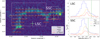 |
Fig. 6 Spectral line shapes of four tracers depicted in filament G37. The spectra contours of 12CO, 13CO, and C18O (3–2) are represented by the blue, yellow, and red lines, respectively, within each block (30ʺ × 30ʺ). The velocity range for these lines is from 47 to 65 km s−1. The background displays the intensity map of 13CO (3–2) at a velocity range of [47,65] km s−1. The right panels display the spectral lines of the large semicircle (LSC) and small semicircle (SSC), which cover the region shown in the left panel. The central velocities of the Hα RRL lines, indicated by the green cross in the left panel, are marked by dotted vertical lines. Each spectral line is distinguished by its respective color. |
4.3 Impact of the magnetic field
The magnetic field is a pivotal factor in the physical evolution of molecular clouds (e.g., Crutcher 2012; Hull & Zhang 2019; Li 2021; Zhao et al. 2024c). It may play a significant role in governing the collapse and fragmentation processes within these clouds, thereby impacting the formation of stars. Furthermore, the magnetic field influences the distribution and movement of gas and dust within the cloud, thereby molding its structure and density. We investigate the role that the magnetic field plays in the formation and evolution of filament G37 at the filament scale. As shown in Fig. 4, the filament-parallel-alignment magnetic field maintains the curved structure of the filament and counteracts the pressure exerted by the expanding H II region, while the clear magnetic field structure was derived using the VGT technique on CO lines with a special velocity range of [51,64] km s−1 in this work (see Appendix C). In detail, the magnetic field exhibits a distinct curvature and aligns parallel to the long axis of filament G37 at the larger semicircular structure of the filament body (see Fig. 4), which is similar to the curved magnetic field squeezed by the surrounding expanding H II regions in bubble N4 and the NGC 6334 molecular complex (Chen et al. 2017; Arzoumanian et al. 2021; Tahani et al. 2023). Due to the resolution of the magnetic field being below the scale of the smaller semicircle, the magnetic field is barely distorted. A future high-resolution observation may unveil the detailed magnetic field structure of the smaller semicircle within filament G37.
As delineated in Sect. 4.1, the observation of material flowing in multiple directions along filament G37 has been noted. The curved magnetic field in filament G37 may play a significant role in guiding the material flows within the filament body. Specifically, the magnetic field aligns parallel to the long axis of filament G37, which coincides with the direction of material flows. This parallel alignment ensures that the material remains unaffected by the magnetic field force, as it flows in the same direction. Conversely, if the orientation of material flow were perpendicular to both the magnetic field and the filament body, the material would experience a magnetic field force opposing its motion. This highlights the ability of the magnetic field to influence and guide the material flow within the filament. By guiding the material flow, the magnetic field actively contributes to the preservation of the curved filament structure.
In contrast to bubble N131, which is influenced by the H II region, the molecular cloud is susceptible to fragmentation and disruption under the pressure exerted by the expanding H II region, as demonstrated by Zhang et al. (2016). However, the magnetic field structure of filament G37 exhibits a curved configuration, where the magnetic field effectively withstands the pressure exerted by the expanding H II region on the filament body. The curved magnetic field structure at the filament scale maintains the filament structure and preserves the structural integrity of filament G37.
We also estimate the mean magnetic field strength and Alfvén Mach number of G37 to be around 23.3 μG and 2.0, respectively (see Appendix C.2 and Table 1). The Alfvén Mach number 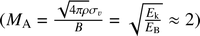 shows that the mean kinetic energy density, Ek , in the filament is slightly larger than the local magnetic energy density, EB. This suggests that the local turbulent motion related to kinetic energy could affect the average magnetic field structure of filament G37.
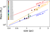 |
Fig. 7 Size and mass of clumps depicted using colored circles and triangles, as shown in Fig. E.1, on the size-mass map. The size refers to the effective diameter of the clumps, which is twice the effective radius. The red and blue dotted lines represent the line masses of 230 and 670 M⊙ pc−1 respectively, which serve as representative values for non-star-forming and star-forming filaments (Li et al. 2016). The orange lines illustrate the relationship associated with massive star formation (Kauffmann et al. 2010). |
 |
Fig. 8 Schematic formation diagram proposed for filament G37. The main structure of filament G37 underwent three evolutionary phases, namely: a) a filament lacking an H II region, b) a filament compressed by an expanding H II region, and c) the formation of filament G37. The structure of the filament is depicted by the blue lines, while the B field is represented by the dashed red lines. The position of the H II region is illustrated by the green graphics. Additionally, the yellow stars and red crosses indicate the locations where star formation was triggered. |
4.4 Star formation in filament G37
As mentioned in Sect. 3.1, the filamentary structure of G37 exhibits bright 8 μm emission, especially in the four dense clumps C1–C4 (see Fig. 1), which has the potential to initiate star formation. To investigate star formation within filament G37, we identified 17 clumps within its filamentary body (see Sect. 3.5). Figure 7 illustrates the correlation between the size and mass of these clumps. The line mass of the clumps in filament G37 consistently surpasses the lower threshold value of the critical mass for star-forming clouds, which is 230 M⊕ pc−1 (Li et al. 2016). This suggests the likelihood of star formation activity within these clumps. Moreover, clumps 1, 2, 12, 16, and 17 exhibit a line mass that exceeds the threshold value for massive star formation, specifically 870 M (Reff pc−1.33) (Kauffmann et al. 2010). These dense clumps (1, 2, 12, 16, and 17) could be considered as potential candidates for massive star formation.
Finding massive clumps in filament G37 is necessary, where it may undergo gravitational collapse. Figs. 1 and E.1 indicate that the candidates for massive star formation, namely clumps 1, 2, 12, 16, and 17, are located within clumps C1, C2, C3, and C4. Furthermore, Fig. 3 reveals a shift in the direction of material flow within filament G37, which occurs at clumps C1, C2, C3, and C4. This suggests that the formation of the dense clumps (C1, C2, C3, and C4) could be attributed to the accretion of material, which results in material flow in various directions within the filamentary structure. Specifically, four dense clumps (1, 2, 12, and 17) situated at the end of filament G37 exhibit the highest masses among all identified clumps (see Table E.1). These results further support the notion that star formation within filament G37 is characterized by end-dominated collapse.
4.5 Schematic formation of filament G37
The schematic formation diagram proposed for filament G37 is depicted in Fig. 8, and highlights three distinct phases. The first phase involves a filament devoid of an H II region, followed by a phase where the filament experiences compression due to the expansion of an H II region. Finally, the formation of filament G37 occurs as a result of magnetic field resistance against the compression exerted by the H II regions. During the initial phase without an H II region, the giant filament maintains a close alignment with the Galactic plane. Previous observations of giant filaments, such as G11, G29, G51, and the Radcliffe Wave, reveal an “S”-shaped morphology within the Milky Way (Li et al. 2013; Wang et al. 2015; Li & Chen 2022; Konietzka et al. 2024). Therefore, we hypothesize that filament G37 initially exhibits a similar “S”-shaped structure, independent of the influence of the expanding H II region (see Fig. 8). The local magnetic field within this filament is observed to be parallel to its body, as documented by Zucker et al. (2018), Soler et al. (2021), and Zhao et al. (2024b). Due to the insufficient evidence available for comparing the ages of filaments and the expansion timescales of H II regions, it is challenging to infer the sequential relationship between filament formation and H II region expansion. In this context, filaments devoid of associated H II regions serve as a control group, which allows for the investigation of the impact of H II regions on filamentary structures.
During the evolutionary phase involving an H II region, the expansion of these regions exerts significant pressure, which results in the distortion of the filament body, as visually demonstrated in Fig. 8. The local magnetic field is also subject to distortion due to the pressure exerted by the expanding H II region, which leads to changes in alignment along the filament body and the formation of curved structures (Chen et al. 2017; Arzoumanian et al. 2021). The compression caused by the expanding H II regions induces the accumulation of gas into dense clumps, which subsequently triggers the process of star formation. As dense clumps accrete material, there are flows of material toward these clumps, which results in multidirectional material flows along the filament body.
As the evolution of filament G37 progresses, the magnetic field within the filament plays a crucial role in counteracting the pressure exerted by the expanding H II region. This interaction continues until a dynamic equilibrium is achieved within the system. Throughout this process, the curved structure of filament G37 undergoes formation and reshaping. The presence of the nearby expanding H II region exerts compression on the filament, which results in a curved filament body and magnetic field structure. This phenomenon triggers the formation of stars and gives rise to the unique occurrence of multidirectional material transportation within filament G37 during its evolutionary stages. The curved magnetic field provides support against the compression exerted by the H II region, thereby maintaining the multiple directions of material flow along the filament body caused by clump accretion, as well as preserving the curved structure of the filament. This physical process, characterized by the interplay between the magnetic field, H II region, and material flows, can persist for a duration of up to 5 Myr.
5 Summary
We conducted an investigation into the dynamics and magnetic field characteristics of filament G37, while also delving into the physical mechanisms underlying its formation. The main results are the following:
Filament G37 exhibits a distinct influence on the motion of material, directing it toward four dense clumps situated at specific locations: C1 and C4, positioned at the ends of the filament, C2, located at the apex of its large semicircular structure, and C3, situated between the two semicircular components. These four clumps present themselves as potential regions for the formation of massive stars;
By employing the 13CO (3–2) spectral line, we estimated the velocity gradients of the material flowing from clumps C2 to C1, C2 to C3, and C3 to C4 to be approximately 0.46, 0.40, and 0.49 km s−1 pc−1, respectively; The observed multidirectional flows of material within these clumps indicate that they may be attributed to the accretion processes that involves these substantial clumps. Filament G37 provides a potential candidate for end-dominated collapse;
The velocity gradients of the two expanding H II regions, which are associated with the large and small semicircles of filament G37, were determined to be 1.10 and 0.54 km s−1 pc−1, respectively. Through the analysis of tracers such as 12CO, 13CO, and Hα RRL, it was observed that the expanded H II region, as traced by Hα RRL, induces compression of the filament gas in the direction of the blue shift. The formation of two semicircular structures within filament G37 is likely attributable to the nearby expanding H II regions. This compression effect could potentially serve as a triggering mechanism for star formation within the filament;
The measured magnetic field obtained from VGT observations revealed a distinctive curved structure, which aligns parallel to the elongated axis of filament G37. Despite the compressive effects exerted by the adjacent H II region, the magnetic field within filament G37 plays a crucial role in preserving its current morphology and directing the flow of material within the filamentary structure. The estimated strength of the magnetic field yielded a value of ~23 μG;
The combined effects of H II region expansion and the curved magnetic field contribute to the unique morphology of G37, which resembles a caterpillar in shape. The timescale for these physical processes within G37 is estimated to be ∼5 Myr.
Acknowledgements
The authors thank the anonymous referee for helpful comments. We thank Dr. Yue Hu and Prof. Alex Lazarian for the VGT code and helpful comments. This work acknowledges the support of the National Key R&D Program of China under grant Nos. 2023YFA1608002, 2023YFA1608204, and 2022YFA1603100, the Chinese Academy of Sciences (CAS) alight of West Chinaâ Program under grant Nos. xbzg-zdsys-202212, the Tianshan Talent Program of Xinjiang Uygur Autonomous Region under grant No. 2022TSYCLJ0005, the Natural Science Foundation of Xinjiang Uygur Autonomous Region under grant No. 2022D01E06, the Xinjiang Key Laboratory of Radio Astrophysics under grant No. 2023D04033, the National Natural Science Foundation of China under grant Nos. 12173075, 12425304, and U1731237, and the Youth Innovation Promotion Association CAS. This research has used NASA’s Astrophysical Data System (ADS).
Appendix A Averaged Spectral Lines of Filament G37
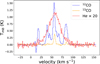 |
Fig. A.1 Three mean spectral lines of 12CO (3–2), 13CO (3–2), and Hα RRL are observed in filament G37. The 12CO (3–2) spectrum is represented by the blue line, while the 13CO (3–2) spectrum is depicted by the orange line. Additionally, the Hα RRL spectrum, with its intensity multiplied by 20 times, is shown by the red line. |
Appendix B Distributions of Central Velocities and Velocity Dispersions of CO
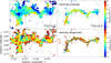 |
Fig. B.1 The distributions of central velocities (top panels) and velocity dispersions (bottom panels) derived from 12CO and 13CO (3–2) spectra. |
Appendix C Magnetic Field Measured with Velocity Gradient Technique
C.1 Velocity Gradient Technique
As depicted in Fig. C.1, six distinct velocity components were identified across various velocity ranges, with Component 4 constituting a segment of filament G37. This observation implies the presence of multiple objects within the line of sight (LOS) direction traversing the multi-spiral arms. The continuum observation is significantly influenced by a substantial number of foreground and background objects originating from different spiral arms. Consequently, measuring the magnetic field of filament G37 using dust-polarized continuum becomes challenging due to the inclusion of these foreground and background objects. The removal of these foreground effects proves to be particularly difficult.
The velocity gradient technique (VGT; González-Casanova & Lazarian 2017; Lazarian & Yuen 2018; Hu et al. 2018) offers a method to measure magnetic fields with multiple velocity components. By utilizing the position-position-velocity (PPV) cubes derived from spectroscopic data, these velocity components can be distinctly separated, allowing for accurate measurements of their respective magnetic fields. Employing the 12CO (3–2) spectral line in conjunction with the VGT technique facilitates the acquisition of a pristine magnetic field structure for filament G37, unaffected by foreground and background interferences.
In this study, the VGT technique is employed for analyzing the magnetic field. This method is predicated on the anisotropy of magneto-hydrodynamic turbulence (Goldreich & Sridhar 1995) and fast turbulent reconnection theories (Lazarian & Vishniac 1999). In order to extract the velocity information from PPV cubes, thin velocity channels denoted as Ch(x,y) were utilized,
 (C.1)
(C.1)
 (C.2)
(C.2)
 (C.3)
where ▽xChi(x,y) and ▽yChi(x,y) are the x and y components of the gradient, respectively. This procedure is executed for pixels exhibiting a spectral line emission with a signal-to-noise ratio (SNR) exceeding 3.
(C.3)
where ▽xChi(x,y) and ▽yChi(x,y) are the x and y components of the gradient, respectively. This procedure is executed for pixels exhibiting a spectral line emission with a signal-to-noise ratio (SNR) exceeding 3.
The orientation of the magnetic field is perpendicular to the velocity gradient, and these velocity gradients must exhibit statistical significance. A technique known as sub-block averaging (Yuen & Lazarian 2017) has been employed to extract velocity gradients from raw gradients within a designated sub-block of interest. Subsequently, a histogram corresponding to the raw velocity gradient orientations, denoted as  , is plotted. The size of this sub-block is fixed at 20×20 pixels, which also dictates the resolution of the final magnetic field. Through the application of sub-block averaging, eigen-gradient maps
  are obtained and used to compute the pseudo-Stokes-parameters Qg and Ug. Consequently, the pseudo-Stokes-parameters Qg and Ug for the inferred magnetic field are constructed based on these parameters by:
 (C.4)
(C.4)
 (C.5)
(C.5)
 (C.6)
where ψg is the pseudo polarization angle. The pseudo polarization angle is perpendicular to the POS orientation angle of the magnetic field: ψB = ψg + π/2.
(C.6)
where ψg is the pseudo polarization angle. The pseudo polarization angle is perpendicular to the POS orientation angle of the magnetic field: ψB = ψg + π/2.
To evaluate the precision of the VGT in tracing magnetic fields, we utilized the PPV cubes from the full velocity channels of the 12CO (3–2) spectral line (see Fig. C.1). This was done to compare the B-field derived from Planck 353 GHz dust polarization with that obtained using VGT. The 12CO (3–2) emission was chosen for this application due to its superior SNRs compared to the 13CO (3–2) emission. Notably, the 12CO (3– 2) emission spans the entire velocity range, encompassing all components along the line of sight. When applied to the VGT method using this 12CO (3–2) emission, the resultant magnetic field encompasses both foreground and background components. Its origin aligns closely with that of the polarized dust continuum, such as the Planck 353 GHz dust polarization. In order to juxtapose the magnetic field as measured by VGT and Planck continuum, we established a sub-block size of 50 50 pixels. This was done to align with the same beam as that utilized by Planck (∼5ʹ). The alignment between the B-field orientations, as detected through polarization θB and VGT ΦB, is characterized by the Alignment Measure (AM, González-Casanova & Lazarian 2017):  . The AM values span a range from −1 to 1. An AM value nearing 1 suggests that ϕB is parallel to ψg, whereas an AM value approaching −1 implies that ϕB is perpendicular to ψg. The uncertainty associated with the AM value, denoted as σAM, can be determined by dividing the standard deviation by the square root of the sample size. This calculation is illustrated in Fig. C.1.
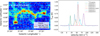 |
Fig. C.1 Comparison of magnetic field measured with VGT for 12CO (3–2) and Planck dust polarization. The comparison of magnetic fields measured with VGT for 12CO (3–2) and Planck dust polarization is shown in the left panel. The orientation of the magnetic field measured using VGT for 12CO (3–2) spectra and dust polarization from Planck is displayed by the red and white vectors, respectively. The integrated intensity of 12CO (3–2) spectral line from −31 to 155 km s−1 is shown in the background. The right panel shows the spectral line of 12CO (3–2) across the full velocity channel, with the six different velocity components represented by different color lines. |
As depicted in Fig. C.1, the AM value reaches up to 0.95 ± 0.01. This indicates that the magnetic field, as measured by VGT in full velocity channels of the 12CO (3–2), closely aligns with that of Planck, exhibiting a mean offset angle of less than 10° between the two types of magnetic field orientation angles. The ability of VGT to trace the magnetic field in filament G37 region is consistent with that of Planck, demonstrating high accuracy. When compared to dust polarization, VGT effectively distinguishes between the foreground and background using a single velocity component (Lazarian & Yuen 2018; Hu et al. 2019; Liu et al. 2022; Hu et al. 2022; Zhao et al. 2022).
C.2 Magnetic Field Strength
Lazarian et al. 2020 introduce a novel method, termed the MM2 technique, for estimating the magnetic field strength Bpos in the plane-of-sky (POS). This technique is specifically applied to both the sonic Mach number and the Alfvén Mach number. The sonic Mach number can be determined using spectral lines and dust temperature measurements:
 (C.7)
where σv,1D is the velocity dispersion obtained from 13CO (3–2), cs is the sonic speed (
(C.7)
where σv,1D is the velocity dispersion obtained from 13CO (3–2), cs is the sonic speed ( , where T is the dust temperature, kB is the Boltzmann constant, μ = 2.37 is the mean molecular weight). Based on the dispersion relation in the direction of the velocity gradient shows a power-law arrangement with MA (Lazarian et al. 2020; Hu et al. 2021), Alfvén Mach number MA could be measured by “top-to-bottom” ratio of the distribution of the channel velocity gradients (VChGs):
 (C.8)
where Tv represents the maximum value of the fitted histogram in the velocity gradient directions, while Bv is the minimum value of that. Using the MM2 technique, magnetic field strength Bpos can be calculated by:
(C.8)
where Tv represents the maximum value of the fitted histogram in the velocity gradient directions, while Bv is the minimum value of that. Using the MM2 technique, magnetic field strength Bpos can be calculated by:
 (C.9)
where the Ω is a geometrical factor (Ω = 1), ρ0 is the volume density estimated by long uniform cylinder model (Fiege & Pudritz 2000; Pattle et al. 2017). MA measured by VChGs is 1.97. The mean value of Bpos in filament G37 is estimated as 23.3 μG. The detail of other physical parameters of filament G37 is shown in Table 1.
(C.9)
where the Ω is a geometrical factor (Ω = 1), ρ0 is the volume density estimated by long uniform cylinder model (Fiege & Pudritz 2000; Pattle et al. 2017). MA measured by VChGs is 1.97. The mean value of Bpos in filament G37 is estimated as 23.3 μG. The detail of other physical parameters of filament G37 is shown in Table 1.
Appendix D Maps of 12CO velocity components
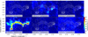 |
Fig. D.1 Velocity-integrated intensity maps of 12CO for each velocity component (see Fig. C.1) are presented in the background. The white contours show the H2 column density, ranging from 1022 to 1022.4 cm−2 with a step of 100.05 cm−2 (Zucker et al. 2018). |
Appendix E Clumps
A total of 17 clumps are identified in filament G37 using the 850 μm continuum, as shown in Fig. E.1 and Table E.1. We utilized the 13CO (3–2) emission of G37 to disentangle clumps, ensuring that it aligned with the shape of the 850 μm emission from cold dust simultaneously. Based on the emission contours from the 850 μm continuum, we identified the positions and structures of the clumps. The mass of each clump was estimated using the H2 column density in conjunction with the clump structure derived from the 13CO (3–2) observations.
Physical Parameters of Clumps.
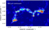 |
Fig. E.1 Identified clumps marked with white crosses in filament G37. Red contours represent the shape of 850 μm emission, which ranges from 50 to 400 mJy beam−1 with steps of 50 mJy beam−1. The white contours correspond to the 13CO (3–2) emission, consistent with Fig. 1. |
References
- Anderson, L. D., Bania, T. M., Balser, D. S., et al. 2014, ApJS, 212, 1 [Google Scholar]
- Anderson, L. D., Luisi, M., Liu, B., et al. 2021, ApJS, 254, 28 [NASA ADS] [CrossRef] [Google Scholar]
- André, P., Men’shchikov, A., Bontemps, S., et al. 2010, A&A, 518, L102 [NASA ADS] [CrossRef] [EDP Sciences] [Google Scholar]
- André, P., Di Francesco, J., Ward-Thompson, D., et al. 2014, in Protostars and Planets VI, eds. H. Beuther, R. S. Klessen, C. P. Dullemond, & T. Henning, 27 [Google Scholar]
- Arzoumanian, D., Furuya, R. S., Hasegawa, T., et al. 2021, A&A, 647, A78 [NASA ADS] [CrossRef] [EDP Sciences] [Google Scholar]
- Arzoumanian, D., Russeil, D., Zavagno, A., et al. 2022, A&A, 660, A56 [NASA ADS] [CrossRef] [EDP Sciences] [Google Scholar]
- Bailer-Jones, C. A. L., Rybizki, J., Fouesneau, M., Demleitner, M., & Andrae, R. 2021, AJ, 161, 147 [Google Scholar]
- Bally, J., Langer, W. D., Stark, A. A., & Wilson, R. W. 1987, ApJ, 312, L45 [NASA ADS] [CrossRef] [Google Scholar]
- Benjamin, R. A., Churchwell, E., Babler, B. L., et al. 2003, PASP, 115, 953 [Google Scholar]
- Bhadari, N. K., Dewangan, L. K., Pirogov, L. E., & Ojha, D. K. 2020, ApJ, 899, 167 [NASA ADS] [CrossRef] [Google Scholar]
- Bhadari, N. K., Dewangan, L. K., Ojha, D. K., Pirogov, L. E., & Maity, A. K. 2022, ApJ, 930, 169 [NASA ADS] [CrossRef] [Google Scholar]
- Brand, J., Massi, F., Zavagno, A., Deharveng, L., & Lefloch, B. 2011, A&A, 527, A62 [NASA ADS] [CrossRef] [EDP Sciences] [Google Scholar]
- Carey, S. J., Noriega-Crespo, A., Mizuno, D. R., et al. 2009, PASP, 121, 76 [Google Scholar]
- Chen, Z., Jiang, Z., Tamura, M., Kwon, J., & Roman-Lopes, A. 2017, ApJ, 838, 80 [Google Scholar]
- Ching, T.-C., Qiu, K., Li, D., et al. 2022, ApJ, 941, 122 [CrossRef] [Google Scholar]
- Churchwell, E., Povich, M. S., Allen, D., et al. 2006, ApJ, 649, 759 [CrossRef] [Google Scholar]
- Churchwell, E., Watson, D. F., Povich, M. S., et al. 2007, ApJ, 670, 428 [NASA ADS] [CrossRef] [Google Scholar]
- Crutcher, R. M. 2012, ARA&A, 50, 29 [Google Scholar]
- Deharveng, L., Lefloch, B., Kurtz, S., et al. 2008, A&A, 482, 585 [NASA ADS] [CrossRef] [EDP Sciences] [Google Scholar]
- Dempsey, J. T., Thomas, H. S., & Currie, M. J. 2013, ApJS, 209, 8 [NASA ADS] [CrossRef] [Google Scholar]
- Dewangan, L. K., Pirogov, L. E., Ryabukhina, O. L., Ojha, D. K., & Zinchenko, I. 2019, ApJ, 877, 1 [Google Scholar]
- Doi, Y., Hasegawa, T., Furuya, R. S., et al. 2020, ApJ, 899, 28 [Google Scholar]
- Doi, Y., Tomisaka, K., Hasegawa, T., et al. 2021, ApJ, 923, L9 [NASA ADS] [CrossRef] [Google Scholar]
- Eden, D. J., Moore, T. J. T., Plume, R., et al. 2017, MNRAS, 469, 2163 [Google Scholar]
- Fiege, J. D., & Pudritz, R. E. 2000, MNRAS, 311, 85 [Google Scholar]
- Field, G. B., Goldsmith, D. W., & Habing, H. J. 1969, ApJ, 155, L149 [NASA ADS] [CrossRef] [Google Scholar]
- Goldreich, P., & Sridhar, S. 1995, ApJ, 438, 763 [Google Scholar]
- González-Casanova, D. F., & Lazarian, A. 2017, ApJ, 835, 41 [CrossRef] [Google Scholar]
- Griffin, M. J., Abergel, A., Abreu, A., et al. 2010, A&A, 518, L3 [EDP Sciences] [Google Scholar]
- Hacar, A., & Tafalla, M. 2011, A&A, 533, A34 [NASA ADS] [CrossRef] [EDP Sciences] [Google Scholar]
- Hacar, A., Tafalla, M., Kauffmann, J., & Kovács, A. 2013, A&A, 554, A55 [NASA ADS] [CrossRef] [EDP Sciences] [Google Scholar]
- Hacar, A., Alves, J., Tafalla, M., & Goicoechea, J. R. 2017, A&A, 602, L2 [NASA ADS] [CrossRef] [EDP Sciences] [Google Scholar]
- Hacar, A., Tafalla, M., Forbrich, J., et al. 2018, A&A, 610, A77 [NASA ADS] [CrossRef] [EDP Sciences] [Google Scholar]
- Hacar, A., Clark, S. E., Heitsch, F., et al. 2023, in Protostars and Planets VII, eds. S. Inutsuka, Y. Aikawa, T. Muto, K. Tomida, & M. Tamura, Astronomical Society of the Pacific Conference Series, 534, 153 [Google Scholar]
- He, Y.-X., Liu, H.-L., Tang, X.-D., et al. 2023, ApJ, 957, 61 [NASA ADS] [CrossRef] [Google Scholar]
- Hou, L. G., & Gao, X. Y. 2014, MNRAS, 438, 426 [Google Scholar]
- Hu, Y., Yuen, K. H., & Lazarian, A. 2018, MNRAS, 480, 1333 [NASA ADS] [CrossRef] [Google Scholar]
- Hu, Y., Yuen, K. H., Lazarian, V., et al. 2019, Nat. Astron., 3, 776 [NASA ADS] [CrossRef] [Google Scholar]
- Hu, Y., Lazarian, A., & Stanimirovic’, S. 2021, ApJ, 912, 2 [NASA ADS] [CrossRef] [Google Scholar]
- Hu, Y., Lazarian, A., & Wang, Q. D. 2022, MNRAS, 513, 3493 [NASA ADS] [CrossRef] [Google Scholar]
- Hull, C. L. H., & Zhang, Q. 2019, Front. Astron. Space Sci., 6, 3 [Google Scholar]
- Hwang, J., Kim, J., Pattle, K., et al. 2022, ApJ, 941, 51 [NASA ADS] [CrossRef] [Google Scholar]
- Jackson, J. M., Rathborne, J. M., Shah, R. Y., et al. 2006, ApJS, 163, 145 [NASA ADS] [CrossRef] [Google Scholar]
- Kauffmann, J., Bertoldi, F., Bourke, T. L., Evans, N. J., I., & Lee, C. W. 2008, A&A, 487, 993 [NASA ADS] [CrossRef] [EDP Sciences] [Google Scholar]
- Kauffmann, J., Pillai, T., Shetty, R., Myers, P. C., & Goodman, A. A. 2010, ApJ, 712, 1137 [NASA ADS] [CrossRef] [Google Scholar]
- Konietzka, R., Goodman, A. A., Zucker, C., et al. 2024, Nature, 628, 62 [Google Scholar]
- Kuhn, M. A., de Souza, R. S., Krone-Martins, A., et al. 2021, ApJS, 254, 33 [NASA ADS] [CrossRef] [Google Scholar]
- Kwon, W., Pattle, K., Sadavoy, S., et al. 2022, ApJ, 926, 163 [NASA ADS] [CrossRef] [Google Scholar]
- Lazarian, A., & Vishniac, E. T. 1999, ApJ, 517, 700 [Google Scholar]
- Lazarian, A., & Yuen, K. H. 2018, ApJ, 853, 96 [NASA ADS] [CrossRef] [Google Scholar]
- Lazarian, A., Pogosyan, D., Vázquez-Semadeni, E., & Pichardo, B. 2001, ApJ, 555, 130 [Google Scholar]
- Lazarian, A., Yuen, K. H., & Pogosyan, D. 2020, arXiv e-prints [arXiv:2002.07996] [Google Scholar]
- Li, H.-B. 2021, Galaxies, 9, 41 [NASA ADS] [CrossRef] [Google Scholar]
- Li, G.-X., & Chen, B.-Q. 2022, MNRAS, 517, L102 [NASA ADS] [CrossRef] [Google Scholar]
- Li, G.-X., Wyrowski, F., Menten, K., & Belloche, A. 2013, A&A, 559, A34 [NASA ADS] [CrossRef] [EDP Sciences] [Google Scholar]
- Li, D. L., Esimbek, J., Zhou, J. J., et al. 2014, A&A, 567, A10 [NASA ADS] [CrossRef] [EDP Sciences] [Google Scholar]
- Li, G.-X., Urquhart, J. S., Leurini, S., et al. 2016, A&A, 591, A5 [NASA ADS] [CrossRef] [EDP Sciences] [Google Scholar]
- Liu, H.-L., Stutz, A., & Yuan, J.-H. 2019, MNRAS, 487, 1259 [Google Scholar]
- Liu, M., Hu, Y., & Lazarian, A. 2022, MNRAS, 510, 4952 [Google Scholar]
- Lu, X., Zhang, Q., Liu, H. B., et al. 2018, ApJ, 855, 9 [Google Scholar]
- Ma, Y., Zhou, J., Esimbek, J., et al. 2023, A&A, 676, A15 [NASA ADS] [CrossRef] [EDP Sciences] [Google Scholar]
- McKee, C. F., & Ostriker, J. P. 1977, ApJ, 218, 148 [NASA ADS] [CrossRef] [Google Scholar]
- Men’shchikov, A., André, P., Didelon, P., et al. 2010, A&A, 518, L103 [Google Scholar]
- Ostriker, J. 1964, ApJ, 140, 1056 [Google Scholar]
- Paron, S., Ortega, M. E., Cunningham, M., et al. 2014, A&A, 572, A56 [NASA ADS] [CrossRef] [EDP Sciences] [Google Scholar]
- Pattle, K., Ward-Thompson, D., Berry, D., et al. 2017, ApJ, 846, 122 [Google Scholar]
- Planck Collaboration III. 2020, A&A, 641, A3 [NASA ADS] [CrossRef] [EDP Sciences] [Google Scholar]
- Planck Collaboration XI. 2020, A&A, 641, A11 [NASA ADS] [CrossRef] [EDP Sciences] [Google Scholar]
- Planck Collaboration XII. 2020, A&A, 641, A12 [NASA ADS] [CrossRef] [EDP Sciences] [Google Scholar]
- Planck Collaboration Int. XXXV. 2016, A&A, 586, A138 [NASA ADS] [CrossRef] [EDP Sciences] [Google Scholar]
- Poglitsch, A., Waelkens, C., Geis, N., et al. 2010, A&A, 518, L2 [NASA ADS] [CrossRef] [EDP Sciences] [Google Scholar]
- Pon, A., Johnstone, D., & Heitsch, F. 2011, ApJ, 740, 88 [NASA ADS] [CrossRef] [Google Scholar]
- Pon, A., Toalá, J. A., Johnstone, D., et al. 2012, ApJ, 756, 145 [NASA ADS] [CrossRef] [Google Scholar]
- Reid, M. J., Dame, T. M., Menten, K. M., & Brunthaler, A. 2016, ApJ, 823, 77 [Google Scholar]
- Reid, M. J., Menten, K. M., Brunthaler, A., et al. 2019, ApJ, 885, 131 [Google Scholar]
- Rigby, A. J., Moore, T. J. T., Plume, R., et al. 2016, MNRAS, 456, 2885 [NASA ADS] [CrossRef] [Google Scholar]
- Schneider, S., & Elmegreen, B. G. 1979, ApJS, 41, 87 [Google Scholar]
- Soler, J. D., Beuther, H., Syed, J., et al. 2021, A&A, 651, L4 [NASA ADS] [CrossRef] [EDP Sciences] [Google Scholar]
- Stil, J. M., Taylor, A. R., Dickey, J. M., et al. 2006, AJ, 132, 1158 [NASA ADS] [CrossRef] [Google Scholar]
- Stutz, A. M. 2018, MNRAS, 473, 4890 [NASA ADS] [CrossRef] [Google Scholar]
- Stutz, A. M., & Gould, A. 2016, A&A, 590, A2 [NASA ADS] [CrossRef] [EDP Sciences] [Google Scholar]
- Tahani, M., Bastien, P., Furuya, R. S., et al. 2023, ApJ, 944, 139 [NASA ADS] [CrossRef] [Google Scholar]
- Umemoto, T., Minamidani, T., Kuno, N., et al. 2017, PASJ, 69, 78 [Google Scholar]
- Urquhart, J. S., Moore, T. J. T., Csengeri, T., et al. 2014, MNRAS, 443, 1555 [Google Scholar]
- Wang, K., Testi, L., Ginsburg, A., et al. 2015, MNRAS, 450, 4043 [Google Scholar]
- Wang, K., Testi, L., Burkert, A., et al. 2016, ApJS, 226, 9 [NASA ADS] [CrossRef] [Google Scholar]
- Wang, J.-W., Koch, P. M., Clarke, S. D., et al. 2024, ApJ, 962, 136 [Google Scholar]
- Whitworth, A. P., Bhattal, A. S., Chapman, S. J., Disney, M. J., & Turner, J. A. 1994, MNRAS, 268, 291 [Google Scholar]
- Williams, J. P., Blitz, L., & McKee, C. F. 2000, in Protostars and Planets IV, eds. V. Mannings, A. P. Boss, & S. S. Russell, 97 [Google Scholar]
- Williams, G. M., Peretto, N., Avison, A., Duarte-Cabral, A., & Fuller, G. A. 2018, A&A, 613, A11 [NASA ADS] [CrossRef] [EDP Sciences] [Google Scholar]
- Wolfire, M. G., Vallini, L., & Chevance, M. 2022, ARA&A, 60, 247 [NASA ADS] [CrossRef] [Google Scholar]
- Yuan, L., Li, G.-X., Zhu, M., et al. 2020, A&A, 637, A67 [EDP Sciences] [Google Scholar]
- Yuen, K. H., & Lazarian, A. 2017, ApJ, 837, L24 [NASA ADS] [CrossRef] [Google Scholar]
- Zernickel, A., Schilke, P., & Smith, R. J. 2013, A&A, 554, L2 [NASA ADS] [CrossRef] [EDP Sciences] [Google Scholar]
- Zhang, C.-P., Li, G.-X., Wyrowski, F., et al. 2016, A&A, 585, A117 [NASA ADS] [CrossRef] [EDP Sciences] [Google Scholar]
- Zhao, M., Zhou, J., Hu, Y., et al. 2022, ApJ, 934, 45 [NASA ADS] [CrossRef] [Google Scholar]
- Zhao, M., Li, G.-X., & Qiu, K. 2024a, ApJ, 976, 209 [Google Scholar]
- Zhao, M., Li, G.-X., Zhou, J., et al. 2024b, ApJ, 961, 124 [Google Scholar]
- Zhao, M., Zhou, J., Baan, W. A., et al. 2024c, ApJ, 967, 18 [Google Scholar]
- Zucker, C., & Chen, H. H.-H. 2018, ApJ, 864, 152 [NASA ADS] [CrossRef] [Google Scholar]
- Zucker, C., Battersby, C., & Goodman, A. 2018, ApJ, 864, 153 [NASA ADS] [CrossRef] [Google Scholar]
- Zucker, C., Goodman, A. A., Alves, J., et al. 2022, Nature, 601, 334 [NASA ADS] [CrossRef] [Google Scholar]
All Tables
All Figures
|
Fig. 1 Structure of filament G37. Panels a, b, and c display the structure of filament G37 at different wavelengths. Panel a presents the submillimeter wavelength emission at 850 μm (Eden et al. 2017). The orange line displays the skeleton of filament G37, which is identified in Li et al. (2016). Four special dense clumps (C1–C4) are denoted by red crosses (see Sect. 3.1). The RGB image at the mid-infrared (Spitzer, GLIMPSE Benjamin et al. 2003; MIPSGAL Carey et al. 2009) is shown in panel b, where red represents 24 μm, green represents 8 μm, and blue represents 3.6 μm. Panel c displays the distribution of continuum emission at 1420 MHz from VGPS (Stil et al. 2006). The cross markers in panels b and c display the position of the young stellar objects (YSOs; Kuhn et al. 2021), which are derived from the mid-infrared range of 3–9 μm obtained from the Spitzer telescope. Panels d and e display the distribution of H2 column density and dust temperature (Zucker et al. 2018). The integrated intensity maps of Hα RRL, 12CO (3–2), and 13CO (3–2) emissions from a velocity of 51 to 62 km s−1 are shown in the panels f, g, and h, respectively. The white contours in all panels show the integrated intensity of 13CO (3–2) from 3 to 15 K km−1 with steps of 3 K km−1. The distribution of excitation temperature derived from 12CO (3–2) emission is shown in panel (i). The spatial resolution of each panel is shown in the lower-right corner. |
| In the text | |
|
Fig. 2 Channel maps of 12CO and 13CO (3–2) emissions for filament G37. The intensity of the 12CO and 13CO (3–2) lines within the velocity range of 51 to 62 km s−1 is depicted by green and red contours, respectively, with a step of 1 km s−1. These contours represent regions where the signal-to-noise ratios of 12CO and 13CO exceed 6σ of the spectral lines, which correspond to approximately 1.9 and 2.1 K km s−1, respectively. The intensity distribution of 12CO emission for each velocity channel is displayed as the gray background of the maps. The skeleton of filament G37 is represented by a cyan line, while four special dense clumps (C1–C4) are denoted by red crosses, which are consistent with those shown in Fig. 1. |
| In the text | |
|
Fig. 3 Position-velocity (P-V) diagram to illustrate the distribution of filament G37, obtained from 13CO emission. The distribution is shown along the filament skeleton, as depicted in Fig. 2, with the dense clumps C1, C2, C3, and C4 (as shown in Fig. 1) represented by the red columns. The x-axis denotes the filament length in unit as pc, while the y-axis shows the velocity, VLSR. The diagram shows vertical dashed red lines for the locations of four dense clumps (C1–C4) and black lines for the velocity gradients. The extra velocity gradient of clump C1 is shown as a dashed line. |
| In the text | |
|
Fig. 4 Magnetic field structure of filament G37 revealed with VGT measurements of 12CO. The orientation of the magnetic field is represented as black vectors. The intensity map of filament G37, derived from 13CO emission, is depicted as white contours (same as Fig. 1). The background of the image corresponds to a mid-infrared three-color map, consistent with Fig. 1. The spatial resolution of the magnetic field measurement using VGT is ~2ʹ, as indicated by a white circle in the bottom-right corner. |
| In the text | |
|
Fig. 5 Position–velocity diagram obtained from Hα RRL observations. In the top panel, the intensity map of Hα RRL emission is displayed in the background, with the filament shape depicted by white contours (same as Fig.1). The filament skeleton is represented by a cyan line. Four key points of filament G37, as shown in Fig.1, are marked by black crosses. The P–V diagrams are derived from two blue lines, namely L1 (middle panel) and L2 (bottom panel), which pass through the top points of the two semicircles. The velocity gradient of the Hα RRL emission is indicated by red lines in the bottom panels, and is obtained by fitting the weighted velocity positions (refer to the black cross in the middle and bottom panels). |
| In the text | |
|
Fig. 6 Spectral line shapes of four tracers depicted in filament G37. The spectra contours of 12CO, 13CO, and C18O (3–2) are represented by the blue, yellow, and red lines, respectively, within each block (30ʺ × 30ʺ). The velocity range for these lines is from 47 to 65 km s−1. The background displays the intensity map of 13CO (3–2) at a velocity range of [47,65] km s−1. The right panels display the spectral lines of the large semicircle (LSC) and small semicircle (SSC), which cover the region shown in the left panel. The central velocities of the Hα RRL lines, indicated by the green cross in the left panel, are marked by dotted vertical lines. Each spectral line is distinguished by its respective color. |
| In the text | |
|
Fig. 7 Size and mass of clumps depicted using colored circles and triangles, as shown in Fig. E.1, on the size-mass map. The size refers to the effective diameter of the clumps, which is twice the effective radius. The red and blue dotted lines represent the line masses of 230 and 670 M⊙ pc−1 respectively, which serve as representative values for non-star-forming and star-forming filaments (Li et al. 2016). The orange lines illustrate the relationship associated with massive star formation (Kauffmann et al. 2010). |
| In the text | |
|
Fig. 8 Schematic formation diagram proposed for filament G37. The main structure of filament G37 underwent three evolutionary phases, namely: a) a filament lacking an H II region, b) a filament compressed by an expanding H II region, and c) the formation of filament G37. The structure of the filament is depicted by the blue lines, while the B field is represented by the dashed red lines. The position of the H II region is illustrated by the green graphics. Additionally, the yellow stars and red crosses indicate the locations where star formation was triggered. |
| In the text | |
|
Fig. A.1 Three mean spectral lines of 12CO (3–2), 13CO (3–2), and Hα RRL are observed in filament G37. The 12CO (3–2) spectrum is represented by the blue line, while the 13CO (3–2) spectrum is depicted by the orange line. Additionally, the Hα RRL spectrum, with its intensity multiplied by 20 times, is shown by the red line. |
| In the text | |
|
Fig. B.1 The distributions of central velocities (top panels) and velocity dispersions (bottom panels) derived from 12CO and 13CO (3–2) spectra. |
| In the text | |
|
Fig. C.1 Comparison of magnetic field measured with VGT for 12CO (3–2) and Planck dust polarization. The comparison of magnetic fields measured with VGT for 12CO (3–2) and Planck dust polarization is shown in the left panel. The orientation of the magnetic field measured using VGT for 12CO (3–2) spectra and dust polarization from Planck is displayed by the red and white vectors, respectively. The integrated intensity of 12CO (3–2) spectral line from −31 to 155 km s−1 is shown in the background. The right panel shows the spectral line of 12CO (3–2) across the full velocity channel, with the six different velocity components represented by different color lines. |
| In the text | |
|
Fig. D.1 Velocity-integrated intensity maps of 12CO for each velocity component (see Fig. C.1) are presented in the background. The white contours show the H2 column density, ranging from 1022 to 1022.4 cm−2 with a step of 100.05 cm−2 (Zucker et al. 2018). |
| In the text | |
|
Fig. E.1 Identified clumps marked with white crosses in filament G37. Red contours represent the shape of 850 μm emission, which ranges from 50 to 400 mJy beam−1 with steps of 50 mJy beam−1. The white contours correspond to the 13CO (3–2) emission, consistent with Fig. 1. |
| In the text | |
Current usage metrics show cumulative count of Article Views (full-text article views including HTML views, PDF and ePub downloads, according to the available data) and Abstracts Views on Vision4Press platform.
Data correspond to usage on the plateform after 2015. The current usage metrics is available 48-96 hours after online publication and is updated daily on week days.
Initial download of the metrics may take a while.