| Issue |
A&A
Volume 693, January 2025
|
|
|---|---|---|
| Article Number | A195 | |
| Number of page(s) | 25 | |
| Section | Cosmology (including clusters of galaxies) | |
| DOI | https://doi.org/10.1051/0004-6361/202451566 | |
| Published online | 17 January 2025 | |
Tomographic cluster clustering as a cosmological probe
1
Dipartimento di Fisica e Astronomia “A. Righi” – Alma Mater Studiorum Università di Bologna, via Piero Gobetti 93/2, 40129 Bologna, Italy
2
INAF – Osservatorio di Astrofisica e Scienza dello Spazio di Bologna, via Piero Gobetti 93/3, 40129 Bologna, Italy
3
INFN – Sezione di Bologna, Viale Berti Pichat 6/2, 40127 Bologna, Italy
4
Max Planck Institute for Extraterrestrial Physics, Giessenbachstr. 1, 85748 Garching, Germany
5
Universitäts-Sternwarte München, Fakultät für Physik, Ludwig Maximilians-Universität München, Scheinerstrasse 1, 81679 München, Germany
6
IFPU, Institute for Fundamental Physics of the Universe, via Beirut 2, 34151 Trieste, Italy
7
INAF-Osservatorio Astronomico di Trieste, Via G. B. Tiepolo 11, 34143 Trieste, Italy
⋆ Corresponding author; This email address is being protected from spambots. You need JavaScript enabled to view it.
Received:
18
July
2024
Accepted:
3
December
2024
Abstract
The spatial distribution of galaxy clusters is a valuable probe for inferring fundamental cosmological parameters. We measured the clustering properties of dark matter haloes from the PINOCCHIO simulations in the redshift range 0.2 < z < 1.0 and with virial masses Mvir > 1014 M⊙ h−1, which reproduce the expected mass selection of galaxy cluster samples. The past light cones we analysed have an angular size of 60 degrees, which approximately corresponds to one-quarter of the sky. We adopted a linear power spectrum model, accounting for non-linear corrections at the scale of baryon acoustic oscillations, to perform a comparative study between 3D and 2D tomographic clustering. For this purpose, we modelled the multipoles of the 3D two-point correlation function, ξ(s); the angular correlation function, w(θ); and the angular power spectrum, Cℓ. We considered observational effects such as redshift-space distortions produced by the peculiar velocities of tracers, and redshift errors. We found that photo-z errors have a more severe consequence on 3D clustering than on 2D clustering, as they affect only the radial separation between haloes and not the angular separation, with a relevant impact on the 3D multipoles. Using a Bayesian analysis, we explored the posterior distributions of the considered probes with different tomographic strategies, in the Ωm − σ8 plane, focusing on the summary parameter S8 ≡ σ8√Ωm/0.3. Our results show that in the presence of large photo-z errors the 2D clustering can provide competitive cosmological constraints with respect to the full 3D clustering statistics, and can be successfully applied to analyse the galaxy cluster catalogues from the ongoing and forthcoming Stage III and Stage IV photometric redshift surveys.
Key words: cosmological parameters / large-scale structure of Universe
© The Authors 2025
 Open Access article, published by EDP Sciences, under the terms of the Creative Commons Attribution License (https://creativecommons.org/licenses/by/4.0), which permits unrestricted use, distribution, and reproduction in any medium, provided the original work is properly cited.
This article is published in open access under the Subscribe to Open model. This email address is being protected from spambots. You need JavaScript enabled to view it. to support open access publication.
1. Introduction
The growth of cosmic structures is governed by long-range gravitational interactions between a large number of systems that behave as tracers of the total matter distribution. Among them, according to the hierarchical model for the cosmic structure formation, galaxy clusters are the latest objects produced by the gravitational infall and the merging of dark matter haloes (Bardeen et al. 1986; Tormen 1998). Reaching masses of up to 1015 M⊙ and radii of the order of a few megaparsecs (McNamara & Nulsen 2007), galaxy clusters are the largest gravitationally bound systems ever formed, located at the nodes of the filamentary cosmic web of large-scale structures (LSSs). These astrophysical objects are multi-component systems, made mainly of dark matter and, to a lesser extent, of baryonic matter in different phases (Voit 2005; Allen et al. 2011). This, together with the variety and number of physical processes involved, including both the non-linear and non-local character of the gravitational force, makes a fully analytical treatment of their formation and evolution not accurate enough, considering the precision of current and future datasets.
For this reason, numerical simulations of the LSS are widely used. Since the most relevant effect in the evolution of large-scale density fluctuations is the gravitational interaction, and since the dominant component is the collisionless dark matter, which does not involve computationally expensive hydrodynamical effects, observations of galaxy clusters can be reproduced, within certain limits, by N-body simulations following only the dark matter component. In fact, the baryonic component has only a negligible effect on the formation and evolution of galaxy clusters, and hence on their clustering properties (Springel et al. 2018; Hernández-Aguayo et al. 2023). In particular, N-body simulations rely on a fiducial cosmology, defined by a certain set of cosmological parameters, and evolve the positions of particles undergoing gravitational interaction over cosmic time (Springel et al. 2001; Springel 2005). Therefore, they require a considerable computational effort to realise a sufficient number of mocks necessary for an adequate statistical treatment of the results.
Despite the advances in computational techniques in recent years, there are still some serious limitations to the generation of cosmological simulations (Garaldi et al. 2020; Vogelsberger et al. 2020; Hernández-Aguayo et al. 2023). An accurate description of the evolution of dark matter perturbations is fundamental for modelling the clustering properties of galaxy clusters. First of all, the study of clustering requires an accurate sampling of the baryon acoustic oscillation (BAO) scale, at around 100 Mpc h−1, which is only possible for large simulations (Monaco 2016). Typical requirements for such mock catalogues imply a volume of about 1 Gpc3 and a mass resolution below 1010 M⊙ h−1, and become even more prohibitive if we want to produce a wide past light cone (PLC) without multiple replications along the same line of sight (Monaco et al. 2013; Monaco 2016). Furthermore, a large number of simulations corresponding to N independent realisations of the Universe are needed to evaluate the associated errors and covariance matrices (Manera et al. 2013; Euclid Collaboration 2021, 2024a). A smaller number of realisations would make the estimate very noisy (Giocoli et al. 2017, 2020), with relevant consequences for the cosmological constraints, also because of the problems related to the inversion of the covariance matrix (Manera et al. 2013; Munari et al. 2017). Thus, approximate methods are often used to obtain independent realisations in a much faster way, by evolving the density fluctuations with the linear theory, and computing higher-order corrections through a perturbative approach (see e.g. Monaco 2016, for a review).
Even though cluster catalogues usually contain sparse statistics, they can be used extensively in cosmological analyses. In particular, cluster clustering has a strong dependence on the amplitude of the mass power spectrum and the matter density parameter of the Universe (see e.g. Sartoris et al. 2016), so it can be successfully exploited to constrain these cosmological parameters (Veropalumbo et al. 2014, 2016; Sereno et al. 2015; Marulli et al. 2018, 2021; Lindholm et al. 2021; Lesci et al. 2022b; Fumagalli et al. 2024; Romanello et al. 2024). It can also significantly improve the constraining power of other cosmological probes, such as weak gravitational lensing of galaxy clusters (Sereno et al. 2015) and number counts (Sartoris et al. 2016), when analysed in combination with them.
Currently, cluster clustering is less studied than the traditional galaxy clustering; nevertheless, it has a series of remarkable advantages. Because they are hosted by the most massive virialised haloes, galaxy clusters are more clustered than galaxies, meaning that they are more biased tracers (e.g. Mo & White 1996; Moscardini et al. 2001; Sheth et al. 2001; Hütsi 2010; Allen et al. 2011). This reduces the effect of redshift-space distortions (RSDs), allowing us to simplify the theoretical model for the clustering signal. In contrast to the galaxy bias, which is usually considered a nuisance parameter in cosmological analysis because it is difficult to model correctly, especially at small comoving separation, the effective bias of galaxy cluster samples can be predicted theoretically (Branchini et al. 2017; Paech et al. 2017; Lesci et al. 2022b) by means of fitting functions that depend on the mass and redshift of the host haloes (e.g. Tinker et al. 2010). Furthermore, the BAO peak in the correlation function of galaxy clusters exhibits a low non-linear damping and is sharper compared to other tracers, in other words it is closer to the predictions of linear theory (Veropalumbo et al. 2016).
Clustering information is often investigated with the three-dimensional (3D) two-point correlation function, ξ(r), measured from the 3D comoving spatial coordinates of the tracers; however, they are not directly accessible and require a cosmological assumption to convert the observed redshifts and angular positions to distances. Since the fiducial cosmology assumed for the measurements might be different from the true one, the measured two-point correlation function might be geometrically distorted by the Alcock-Paczynski (AP) effect (Alcock & Paczynski 1979). A way to avoid this is to extract the clustering signal from the angular positions alone, using the two-point angular correlation function, w(θ), in configuration space, and its harmonic-space counterpart, the angular power spectrum, Cℓ (Hauser & Peebles 1973; Peebles 1973), which do not require any AP correction (Asorey et al. 2012; Salazar-Albornoz et al. 2014; Camera et al. 2018). In principle, these two statistics carry the same cosmological information when the entire spectrum of spherical harmonics and angular scales is considered. However, in practice the limited range of wavelengths that can be probed in the reduced volume of real catalogues affects the correlation function and the power spectrum differently (Ata et al. 2018; Avila et al. 2018). Furthermore, we expect a different response to noise and to potential uncorrected observational or systematic effects, which may lead to complementary though highly correlated estimates of cosmological parameters (Sánchez et al. 2017; Camacho et al. 2019; Romanello et al. 2024).
In this paper we make use of a set of dark matter-only simulations to investigate the clustering properties of massive haloes that reproduce some observational conditions of Stage III surveys, such as the Kilo Degree Survey1 (KiDS; see de Jong et al. 2017; Kuijken et al. 2019), the Dark Energy Survey2 (DES; see Dark Energy Survey Collaboration 2016), the Hyper Suprime-Cam3 (HSC) Subaru Strategic Program (HSC-SSP; see Aihara et al. 2018), and the number of clusters expected in Stage IV surveys, for example Euclid4 (Laureijs et al. 2011; Euclid Collaboration 2020, 2022b, 2025). In particular, our aim is to explore the best strategies for maximising the cosmological information that can be extracted from angular cluster clustering, in both its variants (i.e. w(θ) and Cℓ) to verify if it can provide competitive cosmological constraints with respect to the full 3D study. This tomographic approach examines the clustering properties of individual thickness shells at different depths and requires management with an appropriate binning strategy and handling observational effects, such as RSDs and photo-z errors, in order to quantify their impact on the modelling of the clustering signal.
The paper is organised as follows. In Sect. 2 we describe the dark matter-only simulations, and the adopted angular and mass selections. In Sects. 3, 4, and 5 we present the methods used to measure and model ξ(r), w(θ), and Cℓ. In Sect. 6 we show the result of the Bayesian cosmological analysis. Finally, in Sect. 7 we draw our conclusions and present future perspectives. In Appendix A we quantify the impact of reducing the sky coverage on the angular clustering; in Appendix B we test some simple analytic models for the covariance matrices of the angular correlation function and power spectrum; and in Appendix C we discuss the role of other observational systematics in the estimation of cosmological parameters.
The management of halo catalogues, the measurements of the relevant statistical quantities, the cosmological modelling, and the Bayesian inference presented in this study were performed with COSMOBOLOGNALIB5 (Marulli et al. 2016), a set of free software C++ and Python libraries.
2. Data: PINOCCHIO simulations
The PINpointing Orbit-Crossing Collapsed HIerarchical Objects algorithm (PINOCCHIO; Monaco et al. 2002, 2013; Monaco 2016; Munari et al. 2017) is a fast approximated code for the production of dark matter halo catalogues, which works as follows. A Gaussian density field is generated on a cubic grid and then smoothed on a set of scales R. Following the extended Press & Schechter approach (Press & Schechter 1974; Bond et al. 1991), the ellipsoidal collapse model is then used to estimate the collapse time for each particle on the grid, considering all the smoothing scales. The ellipsoid evolution is approximated by the third-order Lagrangian Perturbation Theory (LPT), which is valid until an orbit crossing event occurs or the ellipsoid collapses on its shortest axis. LPT is also used to calculate halo displacements (Monaco 2016; Munari et al. 2017). When the collapse occurs, the particle is expected to be assigned and incorporated into dark matter haloes or in the filaments between them. This fragmentation is done according to the two main processes that characterise the hierarchical clustering of dark matter haloes, namely matter accretion and merging (Monaco et al. 2002, 2013; Munari et al. 2017).
In this way, the code is able to reproduce the mass and the accretion histories of dark matter haloes (Monaco 2016), with an accuracy for the halo mass function and the linear halo bias of 5% and 10%, respectively, compared to the full N-body simulations (Euclid Collaboration 2021, 2024a; Fumagalli et al. 2022). Even an accuracy of 10% in the power spectrum can be achieved up to z ≈ 1. This means that the LPT is able to reproduce the clustering of haloes, placing them in the right position even at relatively low redshifts (Monaco 2016), with a big advantage in terms of computational time. For these reasons PINOCCHIO has been used for several Euclid preparatory science papers (see e.g. Euclid Collaboration 2021, 2024a, 2022a).
2.1. Dark matter halo catalogues: angular and redshift selections
The PINOCCHIO algorithm simulates cubic boxes with side of L = 3870 Mpc h−1 and periodic boundary conditions, from which replication PLCs are produced, selecting only those dark matter haloes that are causally connected to an observer at the present time (Euclid Collaboration 2021, 2024a). We make use of a set of 1000 PLCs, with an aperture of approximately 60 deg, for a final effective area of 10 313 deg2 (i.e. one-quarter of the sky). To study the clustering properties of haloes, we focus only on one mock, while the full set of PLCs is used to build the random catalogue (see Sect. 2.2) and to evaluate the numerical covariance matrices. The simulations have been run assuming Planck Collaboration XVI (2014) cosmology: Ωm = 0.30711, Ωb = 0.048254, h = 0.6777, ns = 0.96, σ8 = 0.8288 and, unless otherwise stated, this is assumed to compute the clustering models that are compared with the measured quantities and presented in the next figures.
The full catalogue contains haloes in the redshift range 0 < z < 2.5, with virial masses Mvir > 6.7 × 10¹³ M⊙ h−1, sampled with more than 50 particles. However, we focus only on the interval 0.2 < z < 1.0. In real catalogues, a lower limit of 0.1 − 0.2 is expected, due to the reduced lensing power that does not allow a robust lensing analysis, necessary for the mass calibration and the following cosmological exploitation (Bellagamba et al. 2019; Giocoli et al. 2021; Euclid Collaboration 2024b). The upper limit is quite conservative and depends on several considerations. First, it is because our work is in preparation for the analysis of the cluster catalogues form the next KiDS data releases (KiDS-DR4, Kuijken et al. 2019; KiDS-DR5, Wright et al. 2024), where the expected number of clusters at z > 1 is very low and certainly not sufficient for a mass calibration with weak lensing, as already verified in KiDS-DR3, which is extended only up to 0.6 (see e.g. Bellagamba et al. 2019; Giocoli et al. 2021; Lesci et al. 2022a,b; Giocoli et al. 2024; Romanello et al. 2024). Furthermore, the low number of clusters at z > 1 implies that the shot noise term dominates the signal even at the largest angular scales, with non-negligible consequences for the angular power spectrum measurements. Finally, at higher redshifts, we expect a general reduction in the completeness and purity of the cluster sample affecting the robustness of the cosmological analysis.
As explained in Euclid Collaboration (2021), we use a version of the catalogue in which the halo masses have been rescaled in order to match the Despali et al. (2016) halo mass function model, preserving all the fluctuations due to sample variance and shot noise. We also select only haloes with a virial mass larger than 1014 M⊙ h−1, which in good approximation corresponds to the predicted limits of the Stage IV photometric survey cluster selection function (i.e. the limiting cluster mass threshold at z < 2, see e.g. Sartoris et al. 2016). The PLCs are available in both real and redshift space. From the latter, we have also produced mock catalogues by introducing a Gaussian redshift perturbation at the redshift z of each halo, which we will hereafter refer to as photo-z space,
![Mathematical equation: $$ \begin{aligned} P(z_{\rm phot}|z) = \frac{1}{\sqrt{2\pi }\sigma _z} \mathrm{exp}\left[-\frac{\delta z^2}{2\sigma _z^2}\right], \end{aligned} $$](/articles/aa/full_html/2025/01/aa51566-24/aa51566-24-eq2.gif) (1)
(1)
where δz = zphot-z, so that there is no systematic bias in the photometric distribution of the tracers. On the other hand, the standard deviation follows the typical shape for photometric redshift surveys:
 (2)
(2)
The choice of the σz, 0 mimics the characteristics of the observations. In particular, we are interested in broad-band photometric data, for which we set σz, 0 = 0.05, corresponding to the accuracy required for the Stage IV galaxy photometric surveys (see e.g. Sartoris et al. 2016; Euclid Collaboration 2019). In general, the redshift errors associated with cluster detection are smaller than the corresponding errors in galaxy photometry, because they are computed using the information coming from a set of galaxies. For this reason, we should consider the previous value as a worst-case scenario and also adopt a value of σz, 0 = 0.02, which corresponds to the photo-z uncertainty of the KiDS-DR3 cluster catalogue (Maturi et al. 2019). We divide our catalogue either in four redshift bins of binwidth 0.2, or two redshift bins of binwidth 0.4. We limit our analysis to broad redshift bins, several times larger than the photo-z errors, while we do not evaluate the narrow bin case, where Δz ≲ σz, because the redshift subsampling dramatically increases the relative importance of the shot noise over the signal, given the limited number of massive haloes. The chosen binwidths give us a minimum of Δz ≈ 2σz (for Δz = 0.2, σz, 0 = 0.05 and in 0.8 < z < 1.0) and a maximum of Δz ≈ 14σz (for Δz = 0.4, σz, 0 = 0.02 and in 0.2 < z < 0.6).
2.2. Random catalogue
The construction of the random catalogue is fundamental to avoid biases in the measurement of the 3D and angular correlation functions. The random catalogue must take into account all the possible selection effects associated with the construction of the data catalogue, for example irregularities in the mask due to satellite tracks, stars, or the Milky Way plane. In this case, such effects are limited to the angular and redshift distribution of dark matter haloes within the footprint mask of the simulation. So we build our random catalogue by randomly extracting cluster positions and redshifts from the full set of 1000 halo mocks, a number large enough to avoid the presence of a spurious signal of clustering induced by the coordinate repetition. This process is repeated for real, redshift and photo-z space. In this way the random light cone reproduces the angular positions, average redshift and mass distributions of PINOCCHIO, which are independent of the individual realisations. To limit the shot noise effects, the size of the random catalogue is ten times larger than the halo catalogue.
3. 3D two-point correlation function
3.1. Characterisation of the measurement and covariance matrix
The 3D two-point correlation function is defined as the excess probability of finding a pair of haloes in the comoving volume elements δV1 and δV2, at the comoving distance r, relative to that expected from a random distribution. It is expressed by
![Mathematical equation: $$ \begin{aligned} \delta P_{12}(r) = n_V^2\,[1+\xi (r)]\,\delta V_1 \delta V_2, \end{aligned} $$](/articles/aa/full_html/2025/01/aa51566-24/aa51566-24-eq4.gif) (3)
(3)
where nV is the mean number density of objects per unit comoving volume. The two-point correlation function can be measured with the Landy & Szalay (1993) (LS) estimator,
 (4)
(4)
where DD(r), RR(r), and DR(r) are the number of data–data, random–random and data–random pairs with separation r ± Δr/2, respectively, normalised for the total number of data–data, random–random and data–random pairs. Equation (4) provides an unbiased measurement of the two-point correlation function for a number of random objects NR → ∞.
In this work, the 3D two-point correlation is measured in ten linearly equispaced radial bins, in the range 15 − 150 Mpc h−1. At these scales the BAO peak is probed and the halo bias can be approximated as a constant (Manera & Gaztañaga 2011; Mandelbaum et al. 2013; Euclid Collaboration 2024a); in other words, it does not depend on r, but only on redshift and mass. The first three even multipole moments of the 3D correlation function at the redshift-space comoving distance s, ξ0(s), ξ2(s) and ξ4(s), that is, the monopole, quadrupole and hexadecapole, respectively, are shown in Fig. 1 for all the redshift bins of our analysis. Focusing on the monopole, we verified that, as expected, the RSDs cause an enhancement of the clustering signal at all scales, with respect to real space, quantifiable by a factor of 1.1 − 1.2, due to the high mass and thus high bias of the haloes. Conversely, the effect of photo-z errors is dominant, leading to a complete deletion of the BAO feature and to a scale-dependent suppression of the clustering signal, which is particularly important at low scales. This leads to a change in the slope of the correlation function with respect to the unperturbed one. The impact of photo-z errors is even more important on the higher-order multipoles of the correlation function. The quadrupole changes sign, providing a positive contribution, while the hexadecapole, which in redshift space is always compatible with zero for s > 20 Mpc h−1, becomes dominant. From the full set of mocks we also measured the numerical covariance matrix:
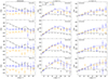 |
Fig. 1. First three even multipoles of the 3D two-point correlation function measured from one PINOCCHIO PLC. The errors are computed as the square root of the diagonal elements of the covariance matrix. We show results for monopoles (white circles), quadrupoles (orange squares), and hexadecapoles (blue triangles). The different columns refer to redshift space with σz = 0, and to photo-z space with σz = 0.02(1 + z) and σz = 0.05(1 + z). The solid lines show the theoretical two-point correlation function multipoles, computed from the power spectrum estimated with CAMB, assuming a linear model with ΣNL = 0 (i.e. without non-linear damping effects at the BAO scale). They include systematic effects, such as RSDs and photo-z damping. The colour of the lines corresponds to the multipoles indicated by the symbols. |
 (5)
(5)
Here a and b refer to the spatial bins involved, while i and j mark the considered redshift bins. The square root of the diagonal elements gives us the error bars shown in Fig. 1. By normalising the covariance matrix with its diagonal elements, we can obtain the correlation matrix,
 (6)
(6)
which is shown in Fig. 2 for real space, redshift space and photo-z space measurements. The cross-correlation between different redshift bins is compatible with zero even in the presence of photo-z errors, which cause an overlap between the redshift distributions of the haloes, thus it is not reported and we only investigate the auto-correlation within the same redshift bin. In particular, if we focus on the block diagonal submatrices, which represent the auto-correlation of the multipoles between different radial bins, we find non-negligible off-diagonal terms that are large even when the bins are widely separated. This is a known feature, reflecting the fact that the 3D and angular correlation functions, in configuration space, are more correlated than their power spectrum counterparts in Fourier and spherical harmonic space (Crocce et al. 2011; Chan et al. 2022). However, this correlation decreases with both increasing multipoles and redshift. Moreover, while we see no significant difference between real and redshift space, due to the limited impact of RSDs, we find a significant reduction in the correlation with larger photo-z errors, which is also common to the w(θ) covariance matrices (see Sect. 4.1).
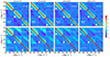 |
Fig. 2. Numerical correlation matrices of the 3D two-point correlation function first three even multipoles, derived from 1000 PLCs. The corresponding colour-bar is shown on the right. In the top panels the red diagonal separates the results for real space (upper triangles) and redshift space, with σz = 0 (lower triangles). In the bottom panels the red diagonal separates the results in photo-z space, where RSDs are included, for photo-z errors given by σz = 0.02(1 + z) (upper triangles) and σz = 0.05(1 + z) (lower triangles). In each panel the horizontal and vertical white solid lines separate the correlation sub-matrices of the monopole ξ0(r), the quadrupole ξ2(r), and the hexadecapole ξ4(r), and their corresponding cross-correlations. |
On the other hand, from the inspection of the off-block diagonal terms, we can assess the cross-correlation between different multipoles. As expected, in real space, it is consistent with zero for every considered redshift bin, since there is no contribution from quadrupole and hexadecapole. In redshift and photo-z space, the correlation progressively reduces at large z and it is generally higher between adiacent multipoles. In particular, in presence of photo-z errors, we find that positive deviations of ξ0(s) and ξ2(s) from their mean value are associated with positive deviations in ξ2(s) and ξ4(s), if s0 < s2 or s2 < s4, respectively, while for s0 > s2 and s2 > s4 we find an anti-correlation.
3.2. Modelling the 3D two-point correlation function
Given the density contrast field δ(x)≡δρ(x)/ρb, where ρb is the mean background density, it is possible to define the 3D two-point correlation function,
 (7)
(7)
as the expectation value, ⟨…⟩, of the product of the overdensities positioned at points x1 and x2. For the cosmological principle we can assume isotropic density fluctuations, so that ξ(x1, x2) = ξ(r), which means that it depends only on the distance between the sources, r ≡ |x2 − x1|, and not on their positions. Dark matter haloes can be treated as biased tracers of the underlying matter distribution. Therefore, in the range of masses and linear scales that we are analysing this translates into a linear relationship between the halo and the dark matter density contrast, δh(x) and δ(x):
 (8)
(8)
through a scale-independent bias, bh(z), which implies a halo–halo correlation function, ξhh(r) = bh2(z)ξ(r). Since the power spectrum is the Fourier transform of the correlation function, the linear bias can be expressed in the same way, as the ratio between the power spectra: Phh(k) = bh2P(k).
For P(k) we adopt the linear model, but taking into account the non-linear damping effects which produce a smearing of the two-point correlation function at the BAO peak, summarised in the parameter ΣNL, which is left free to vary. Therefore, following Veropalumbo et al. (2016), Avila et al. (2018) and Chan et al. (2018), among others, we modelled P(k) as
![Mathematical equation: $$ \begin{aligned} P(k) = [P_{\rm lin}(k)-P_{\rm nw}(k)]e^{-k^2\Sigma ^2_{\mathrm{NL}}/2}+P_{\rm nw}(k), \end{aligned} $$](/articles/aa/full_html/2025/01/aa51566-24/aa51566-24-eq10.gif) (9)
(9)
where Plin(k, z) = Plin(k, 0)D2(z) is provided by CAMB (Lewis et al. 2000), and is strictly valid only in linear theory (Blake et al. 2007), D(z) is the linear growth factor, normalised so that D(0) = 1, while Pnw(k) is the power spectrum without the BAO peak, as obtained by the parametrisation presented in Eisenstein & Hu (1998). The real-space correlation function, ξ(r), is then obtained by Fourier transforming the corresponding power spectrum.
To compare ξhh(r) to the 3D correlation measured from the simulations, we consider the effective bias (i.e. the linear bias integrated above our mass threshold). In practice, beff is the halo bias weighted with the halo mass function,
 (10)
(10)
where  is computed with the parametrisation provided by Despali et al. (2016), which was also used for the calibration of the halo mass function of the PINOCCHIO catalogues, as mentioned in Sect. 2.1. For b(M, z) we adopt the theoretical halo-bias model presented in Tinker et al. (2010).
3.2.1. Redshift-space and geometric distortions
In real galaxy and cluster photometric surveys, the observed redshifts of the tracers, zobs, are linked to the cosmological redshifts, zc, as (neglecting all relativistic corrections and redshift measurement uncertainties)
 (11)
(11)
where zc is related to the cosmological Hubble flow, while the second term is due to the line-of-sight peculiar velocities, v∥, which introduce distortions in the clustering signal if ignored. We neglect the so-called fingers-of-God (FoG) effect, generated by the non-linear dynamics at small scales (Jackson 1972; Peacock et al. 2001), while we consider the large-scale squashing determined by the coherent infall towards collapsing structures, namely the Kaiser effect (Kaiser 1984). In the latter case, the linear regime velocity field can be directly determined from the density field and the anisotropic redshift space power spectrum can be parametrised as
 (12)
(12)
where P(k) is computed with Eq. (9), f ≡ dlnD/dlna is the linear growth rate and μ is the cosine of the angle between k and the line of sight. Here, the fμ2 term reproduces at all scales the coherent motions of large-scale structure, which acts as a bulk flows from underdense to overdense regions. RSDs in the Kaiser limit are proportional to the parameter β = f/beff, thus their effect is less important in more clustered (i.e. in large mass haloes).
The anisotropic redshift–space 3D correlation function, ξhh(s, μ), can be expressed in terms of multipoles ξℓ(s) and Legendre polynomials Lℓ(μ) (Hamilton 1992):
 (13)
(13)
To model the multipoles, we can start from the expansion of the anisotropic power spectrum in Eq. (12),
 (14)
(14)
where μ is the line-of-sight cosine, while k′ and μ′ are rescaled according to the prescription of Beutler et al. (2014)
![Mathematical equation: $$ \begin{aligned} k^{\prime }=\frac{k}{\alpha _{\perp }}\left[1+\mu ^2\left(\frac{\alpha _{\perp }^2}{\alpha _{\Vert }^2}-1\right)\right]^{1 / 2}, \end{aligned} $$](/articles/aa/full_html/2025/01/aa51566-24/aa51566-24-eq17.gif) (15)
(15)
and
![Mathematical equation: $$ \begin{aligned} \mu ^{\prime }=\mu \frac{\alpha _{\perp }}{\alpha _{\Vert }}\left[1+\mu ^2\left(\frac{\alpha _{\perp }^2}{\alpha _{\Vert }^2}-1\right)\right]^{-1/2}. \end{aligned} $$](/articles/aa/full_html/2025/01/aa51566-24/aa51566-24-eq18.gif) (16)
(16)
The geometric distortions are corrected through
 (17)
(17)
where Hfid(z) and  represent the fiducial Hubble parameter and angular diameter distance, respectively, while rs(zd) is the sound horizon at the drag redshift, zd, and
  is its fiducial value. Then, the multipoles ξℓ are expressed as
 (18)
(18)
where i is the imaginary unit and jℓ(x) is the ℓth order spherical Bessel function. The monopole can be simply written as a function of the real-space correlation function, ξ(r):
![Mathematical equation: $$ \begin{aligned} \xi _{\mathrm{hh,}0}(s) = \left[b^2_{\mathrm{eff}}+\frac{2}{3}b_{\mathrm{eff}}f+\frac{1}{5}f^2 \right]\xi (\alpha r). \end{aligned} $$](/articles/aa/full_html/2025/01/aa51566-24/aa51566-24-eq23.gif) (19)
(19)
Here α is the parameter that corrects for the geometric distortions,
 (20)
(20)
where DV is the average distance at redshift z, and DVfid is the same quantity, but estimated at the fiducial cosmology. Their ratio rescales the distances at which the correlation function model is evaluated.
3.2.2. Photo-z errors
Redshift errors introduce a σz term in Eq. (11), perturbing the distance measurements along the line of sight:
 (21)
(21)
Following the approach presented in Blake & Bridle (2005), Asorey et al. (2012), Pezzotta et al. (2017), we can modify Eq. (12) as
 (22)
(22)
The exponential factor in Eq. (22) affects the clustering signal in a way similar to that of random peculiar motions (Marulli et al. 2012). It translates in a Gaussian damping term, analogous to the FoG effect (García-Farieta et al. 2020), which causes a scale-dependent suppression of the signal for k > 1/σ, where σ quantifies the impact of photometric random perturbations on cosmological redshifts. In particular,
 (23)
(23)
where c is the speed of light and H(z) is the Hubble parameter. This is equivalent to assuming that the redshift errors follow a Gaussian distribution with zero mean and with dispersion given by σz (Hütsi 2010).
The monopole of the 3D correlation function can be computed after integrating over μ, following the redshift-space model presented in Sereno et al. (2015), and used by Lesci et al. (2022b):
 (24)
(24)
Here different terms of the correlation function are obtained from the inverse Fourier transforms of the corresponding power spectra. In particular,
 (25)
(25)
![Mathematical equation: $$ \begin{aligned} P{\prime \prime }(k) = \frac{f}{(k\sigma )^3}P(k)\left[ \frac{\sqrt{\pi }}{2}\mathrm{erf}(k\sigma )-k\sigma \mathrm{exp}(-k^2\sigma ^2)\right], \end{aligned} $$](/articles/aa/full_html/2025/01/aa51566-24/aa51566-24-eq30.gif) (26)
(26)
and
![Mathematical equation: $$ \begin{aligned} P^{\prime \prime \prime } (k)&= \frac{f^2}{(k\sigma )^5} P(k) \left\{ \frac{3\sqrt{\pi }}{8}\mathrm{erf}(k\sigma ) \right.\nonumber \\&\pm \left. \frac{k\sigma }{4} [2(k\sigma )^2+3] \mathrm{exp}(-k^2\sigma ^2) \right\} , \end{aligned} $$](/articles/aa/full_html/2025/01/aa51566-24/aa51566-24-eq31.gif) (27)
(27)
respectively. We note that in real space P″(k) and P″′(k) are both zero. Finally, the multipoles are simply computed by using the power spectrum of Eq. (22) into the Eqs. (14) and (18).
4. Angular two-point correlation function
4.1. Characterisation of the measurement and covariance matrix
The angular correlation function measures the average correlation between any two objects placed in the solid angle elements δΩ1 and δΩ2, separated by an angle θ. It can be defined in a completely analogous way with respect to its full 3D counterpart,
![Mathematical equation: $$ \begin{aligned} \delta P_{12}(\theta ) = n_{\Omega }^2[1+{ w}(\theta )]\delta \Omega _1 \delta \Omega _2, \end{aligned} $$](/articles/aa/full_html/2025/01/aa51566-24/aa51566-24-eq32.gif) (28)
(28)
where nΩ is the mean number of objects per unit solid angle. We measure w(θ) in ten linearly spaced bins with the LS estimator (Landy & Szalay 1993),
 (29)
(29)
where DD(θ), RR(θ), and DR(θ) are the normalised number of data–data, random–random, and data–random pairs in the angular bin θ ± Δθ/2, respectively. The advantage of the angular correlation measurement is that it requires only the random catalogue in RA and Dec, without any information about the redshift distribution. This allows us to greatly simplify the measurement process.
We choose angular ranges that vary as a function of redshift. In particular, we explore scales above the maximum angular size obtained from the virial radii of the halo sample, while for z > 0.4 we adopt a more conservative limit of 20 arcmin, in order to exclude comoving separations below 10 Mpc h−1, where there is a significant deviation of the clustering signal from the linear model prediction, both in ξ(r) and in w(θ). In Fig. 3 we show our results for each redshift bin. For graphical requirements, we plot θ w(θ) and we set independent x-axes. The same angle covers greater physical distances as the redshift increases. This results in a shift of w(θ) towards smaller scales. As for the 3D case, the RSDs have only a slight impact. Again, we find the dominant effect in the photo-z space, where photo-z errors cause a drop in the angular clustering.
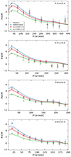 |
Fig. 3. Angular two-point correlation function, measured from one PINOCCHIO PLC. The errors are computed as the square root of the diagonal elements of the covariance matrix. We show results for redshift space with σz = 0 (blue circles), and for photo-z space with RSDs, for photo-z errors equal to σz = 0.02(1 + z) (red squares) and σz = 0.05(1 + z) (green triangles). The solid lines show the theoretical two-point correlation function, computed from the power spectrum estimated with CAMB, assuming a linear model with ΣNL = 0 (i.e. without non-linear damping effects at the BAO scale). They include RSDs, and their colours correspond to the photo-z damping indicated by the symbols. |
It is noteworthy that, in contrast to the 3D case, the BAO feature is preserved, suffering only a minor degradation when passing to σz, 0 = 0.02 − 0.05. This is because redshift uncertainties affect only the radial distances and not the transverse angular ones. Thus, their effect is greater on the reconstruction of the 3D correlation function or power spectrum, which depend on r or k, rather than on their angular counterparts.
In Fig. 4 we show the numerical covariance matrices, derived from the full set of 1000 PLCs. Their features are similar to the 3D case: no significant level of correlation between different redshift bins, even after the introduction of photo-z errors; positive auto-correlation between different radial bins, which decreases progressively with redshift and with larger photo-z errors.
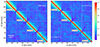 |
Fig. 4. Numerical correlation matrices of the angular two-point correlation function derived from 1000 PLCs (see colour-bar on the right). Left: results for real space (upper triangle) and redshift space, with σz = 0 (lower triangle). Right: results in photo-z space, where RSDs are included, for photo-z errors given by σz = 0.02(1 + z) (upper triangle) and σz = 0.05(1 + z) (lower triangle). In each panel the horizontal and vertical white solid lines separate the cross-correlation sub-matrices measured between different redshift bins. |
4.2. Modelling the angular two-point correlation function
The study of angular clustering considers the projection of the spatial halo density field onto the celestial sphere, in a given direction of the sky  :
:
 (30)
(30)
Here ϕi(z) is the normalised selection function in the ith redshift bin. Given the projected density field, the angular correlation function can be defined as (Peebles 1973)
 (31)
(31)
and can be computed as the projection of the 3D spatial correlation function, ξ(s),
 (32)
(32)
where  , μ is the same of Eq. (12) and takes the form
  , and r(z) is the comoving distance at redshift z. The case i = j refers to the auto correlation, while i ≠ j to the cross correlation between different redshift bins. RSDs can be naturally incorporated, by including a multiplicative factor at the level of the power spectrum.
The anisotropic redshift-space 3D correlation function, ξhh(s, μ) can be expressed with an infinite series of even multipoles, ξℓ(s), and Legendre polynomials, Lℓ(μ), such that ξ(s, μ) = ∑ℓξℓ(s)Lℓ(μ), as in Eq. (13). Most of the information is contained in the monopole (García-Farieta et al. 2020), but following Salazar-Albornoz et al. (2014), to avoid systematics, we include also the correction given by the quadrupole. We do not account for successive terms, because we have verified that the hexadecapole contribution is negligible, for the adopted P(k) model.
4.3. Redshift selection function model
The radial selection function, ϕ(z), encodes the probability of including a halo in a given redshift bin. In the absence of redshift errors, ϕ(z) reduces to the true underlying redshift distribution,
 (33)
(33)
where
 (34)
(34)
which is related to the survey area, Ωsky, in our case 10 313 deg2. Equation (34) has a cosmological dependence given by the derivative of the comoving volume,  , and by the halo mass function, dn(M, z)/dM, for which we use the functional form provided by Despali et al. (2016).
The selection function in a given redshift bin is determined by the window function W(z),
 (35)
(35)
which in our redshift-space mock can simply be considered as a top-hat function in the chosen redshift shell. Complications arise when we consider photometric redshifts, which have non-negligible errors that can significantly alter the clustering signal. When dealing with angular clustering, redshift uncertainties enter into the redshift selection function as a modification of the halo redshift distribution, rather than as a damping term at the level of the power spectrum, as we have seen in Sect. 3.2.2 (Asorey et al. 2012). So we need to consider the conditional probability P(z|zphot) of having a halo at the true redshift, z, given the photometric redshift, zphot. The selection of an object in a photometric redshift bin is determined by a top-hat window function in zphot, reflecting the adopted binning strategy (Asorey et al. 2012):
 (36)
(36)
Here zmin and zmax represent the limits of our photometric redshift interval, respectively.
Thus, the normalised redshift distribution in the i-th photometric bin is obtained with the convolution (Budavári et al. 2003; Crocce et al. 2011; Hütsi et al. 2014)
 (37)
(37)
where P(zphot|z) is given by Eq. (1). This quantity can assume a complicated form, depending on several parameters, including the fraction of catastrophic outliers, fout, namely systems with severely misestimated photometric redshifts (e.g. Hütsi et al. 2014; Euclid Collaboration 2020). For example, in optically selected clusters, if the catastrophic outlier fraction of the member galaxies is large, the cluster properties could be altered, as an increased number of false detections or a large uncertainty in the redshift estimate (Euclid Collaboration 2019). However, in our case, for construction, a simple Gaussian distribution is assumed, whose mean is z, while the standard deviation is equal to σz = σz, 0(1 + z), with σz, 0 = 0 − 0.02 − 0.05, depending on the photo-z errors of our mocks. This choice was also adopted in Romanello et al. (2024) and is motivated by the fact that we do not expect a significant shift in the estimated cluster redshift of real catalogues, assuming the outlier rate of recent photometric surveys (e.g. Hildebrandt et al. 2017). Finally, the redshift distribution in the ith redshift bin is expressed by
 (38)
(38)
In Fig. 5 we show the redshift distribution of haloes, in 0.2 < z < 1.0. For the sake of simplicity, we report only two extreme cases. The coloured, hatched histogram, represented by a solid thick line, shows the real-space redshift distribution, while the dashed histogram shows the photo-z space redshift distribution, in which the redshifts are perturbed with σz, 0 = 0.05. Due to this perturbation, some haloes leave their redshift bin, while others enter it. The net effect would be zero in the case of a uniform initial distribution in z. However, given the initial shape of the dN/dz (solid line in Fig. 5), that can be modelled by integrating the Despali et al. (2016) mass function with Eq. (34), between the minimum and maximum masses of the mock catalogue, the introduction of photo-z errors determines a flattening of the overall distribution, leading to a migration of haloes from the most populated to the less populated bins. The result is shown with the partially overlapping dashed curves in Fig. 5.
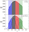 |
Fig. 5. Redshift distribution of dark matter haloes, dN/dz, from a single realisation of PINOCCHIO PLC, with an angular radius of approximately 60 deg, in the redshift range 0.2 < z < 1.0. The coloured hatched histogram represented with a solid line shows the real-space redshift distribution, while the dashed histogram shows the photometric distribution, after the introduction of a Gaussian perturbation with σz = 0.05(1 + z). The light shaded regions give the limits of the photometric redshift bins of our tomographic analysis, with Δz = 0.2. The solid line gives the true dN/dz in the window function W, derived by integrating the halo mass function of Despali et al. (2016), assuming the cosmological parameters of the simulation. The dashed lines are derived through Eq. (38) and show the expected halo distribution in the ith redshift bin, selected by W. |
5. Angular power spectrum
5.1. HEALPIX pixelated map
Given the angular position and redshift of the haloes, we generate tomographic density maps, using the HEALPIX pixelisation scheme (Górski et al. 2005), with a resolution of Nside = 512. The smoothing of the density field within equal area pixels results in a loss of information for ℓ ≳ 1500, namely the corresponding pixel size. However, this value is well above the upper limits in which the measurements are made (i.e. ℓ = 150 − 200), depending on the redshift bin. In each pixel, the density contrast, δh, p, is measured as
 (39)
(39)
where nh, p is the halo count in the pth pixel, while  is the average halo count computed within the circle of 60 degrees angular radius that delimits our PLCs.
5.2. Angular power spectrum estimator
The angular power spectrum can be obtained from the projected density field expressed in Eq. (30). The density contrast, being defined on a 2D sphere, can be expanded into a series of spherical harmonics, Yℓm, computed at the direction on the sky  :
:
 (40)
(40)
Here aℓm are the harmonic coefficients. The orthonormality of the Yℓm implies that the last equation can be reversed and approximated for a pixellised map:
 (41)
(41)
The angular power spectrum can then be easily evaluated with an estimator already introduced by Hauser & Peebles (1973), Peebles (1973) and widely used in the literature (e.g. Balaguera-Antolínez et al. 2018),
![Mathematical equation: $$ \begin{aligned} K^{ij}_\ell =\frac{1}{{ w}^2_\ell }\left[\frac{1}{f_{\mathrm{sky}}(2\ell +1)}\sum _{m=-\ell }^{+\ell } |a^i_{\ell m}a^{*j}_{\ell m}|- \frac{\Omega _{\rm sky}}{N_{\mathrm{h}}}\delta ^{ij}_{\rm K}\right], \end{aligned} $$](/articles/aa/full_html/2025/01/aa51566-24/aa51566-24-eq52.gif) (42)
(42)
where wℓ is the HEALPIX pixel window function, which corrects for the loss of power due to the pixelisation, fsky is the sky fraction covered by our PLC, Nh is the number of haloes in the considered redshift bin and  is the Kronecker delta that cancels the shot noise term in the cross-correlation case.
The results are shown in Fig. 6. Coloured symbols refer to the measurements in redshift and photo-z space, while error bars are estimated as the square root of the diagonal of the covariance matrix. RSDs have an impact that increases with redshift, and affect the measured angular power spectrum at large angular scales, corresponding to ℓ < 10 − 40, depending on the redshift bin. However, since we select haloes with large virial masses, their effect is generally negligible in the angular range of our analysis. On the other hand, photo-z errors cause a general suppression of the clustering signal and need to be modelled in the same way as for the angular correlation function. We averaged the Cℓs in bands of Δℓ = 20, which allowed us to make the covariance matrix more diagonal, since it is blurred due to the partial sky coverage, and to reduce its size (Blake et al. 2007; Balaguera-Antolínez et al. 2018; Loureiro et al. 2019). In Fig. 7 we show the correlation matrices, estimated by substituting Cℓs in Eq. (5). As expected, assuming that the aℓms follow a Gaussian distribution, different multipoles of the power spectrum are independent, and the correlation in spherical harmonics space is lower than in configuration space (see Appendices B.1 and B.2).
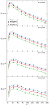 |
Fig. 6. Angular power spectrum, measured from one PINOCCHIO PLC. The errors are computed as the square root of the diagonal elements of the covariance matrix. We show results for redshift space with σz = 0 (blue circles), and photo-z space with RSDs for photo-z errors equal to σz = 0.02(1 + z) (red squares) and σz = 0.05(1 + z) (green triangles). The solid lines show the theoretical angular power spectrum, computed from the power spectrum estimated with CAMB, assuming a linear model with ΣNL = 0 (i.e. without non-linear damping effects at the BAO scale). They include RSDs, and their colours correspond to the photo-z damping indicated by the symbols. |
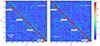 |
Fig. 7. Numerical correlation matrices of the angular power spectrum, derived from 1000 PLCs (see colour bar on the right). Left: results for real space (upper triangle) and redshift space, with σz = 0 (lower triangle). Right: results in photo-z space where RSDs are included, for photo-z errors given by σz = 0.02(1 + z) (upper triangle) and σz = 0.05(1 + z) (lower triangle). In each panel the horizontal and vertical white solid lines separate the cross-correlation sub-matrices measured between different redshift bins. |
5.3. Shot noise correction
The second term in the right-hand side of Eq. (42) quantifies the part of the measured signal related to the discreteness distribution of tracers, which does not contain clustering information. This is called shot noise and must be removed in order to correctly estimate the angular power spectrum. We have seen that the shot noise can be modelled as the ratio between the survey area Ωsky and the number of haloes Nh in a given redshift bin, while it is equal to zero in the cross-correlation case.
Depending on the number of objects, the shot noise is sensitive to the adopted binning strategy. It plays a minor role in large galaxy catalogues, while it generally becomes important when working with smaller catalogues of clusters. In our case, due to the M > 1014 M⊙ h−1 mass cut, we have approximately 104 haloes in each redshift bin, between 0.2 < z < 1.0. This fact enhances the relative importance of the shot noise, which becomes completely dominant over the signal even at relatively large angular scales. For this reason, we set the upper limit of our measurements at the scale where it is about twice as large as the signal, which corresponds to ℓ = 150 − 200, depending on the redshift bin. These values are equivalent to the lower limits θ = 1.2 deg and 0.9 deg, respectively. Thus, the final angular range of the Cℓ analysis is smaller than that considered for w(θ).
The Poissonian approximation assumes point-like objects and so may not hold for finite-size tracers, such as haloes. We expect mass-dependent deviations from Ωsky/Nh, due to the halo exclusion, namely the fact that it is not possible for the distance between two haloes to be smaller than the sum of their physical sizes, and non-linear effects (Giocoli et al. 2010; Baldauf et al. 2013; Paech et al. 2017). In Romanello et al. (2024) we verified that this approximation holds for galaxy clusters in the angular range ℓ ∈ [10 − 175], which roughly corresponds to the angular scales we are focusing on. In particular, we use a method already introduced in Ando et al. (2018), Makiya et al. (2018) and Ibitoye et al. (2022), for the analysis of the galaxy-galaxy angular power spectrum. In practice, we randomly split our PLC into two sub-catalogues each containing, by construction, roughly the same number of dark matter haloes. Then we build the corresponding density maps, δ1, h and δ2, h, which are slightly different in each realisation, being based on a random extraction process. By combining them, we can build the half-sum,  , and the half-difference density fluctuation maps,
  . The half-sum map contains both signal and noise, while only the shot noise contributes to the half-difference map, where the signal, common to both δ1, h and δ2, h, cancels out. We estimate CℓHS and CℓHD, the half-sum and the half-difference power spectra, respectively, which are then averaged over 100 different realisations. In Fig. 8 we summarise the result. The purple squares show the averaged CℓHD and the purple shaded regions indicate the stardard deviation of the estimated shot noise. Interestingly, we notice that the theoretical Poissonian approximation, which we indicate with the cyan, horizontal lines, is valid in every redshift bin of our analysis and in a wide range of multipoles, excluding the largest angular scales, namely ℓ ≲ 10, where the measured shot noise is lower than the theoretical expectation. This method shows us that we can simply subtract the Poissonian noise from the measured Cℓ, as in Eq. (42), and that the uncertainties related to this process can be quantified, and eventually included as a free parameter of the power spectrum model. Following Loureiro et al. (2019) and Romanello et al. (2024), we include in the theoretical model a nuisance parameter, such that Cℓii → Cℓii + 𝒮i. Then, 𝒮i is forward modelled with a uniform prior centred in zero, and is allowed to vary within a multiple of the standard deviation estimated in the ith redshift bin.
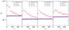 |
Fig. 8. Shot noise estimation over 100 realisations, using one realisation of the PINOCCHIO PLCs, in four redshift bins in the range 0.2 < z < 1.0 (panels from left to right). The red circles represent the angular power spectrum of the half-sum (HS) maps, which include the contribution of both signal and noise. The purple squares instead show the angular power spectrum of the half-difference (HD) maps, which provide a direct estimate of the shot noise, with their average (purple dashed line) and standard deviation (purple shaded band) in agreement with the theoretical Poissonian value (cyan solid line). |
5.4. Modelling the angular power spectrum
The angular power spectrum is modelled from the radial projection of the spatial power spectrum, using the relationship (Padmanabhan et al. 2007; Thomas et al. 2011; Asorey et al. 2012; Camacho et al. 2019)
![Mathematical equation: $$ \begin{aligned} C_{\ell }^{ij} = \frac{2}{\pi } \int \, \mathrm{d}k \, k^2 P(k) \left[ \Psi _{\ell }^i(k) +\Psi ^{i, r}_\ell (k) \right]\left[ \Psi _{\ell }^j(k) +\Psi ^{j, r}_\ell (k) \right], \end{aligned} $$](/articles/aa/full_html/2025/01/aa51566-24/aa51566-24-eq56.gif) (43)
(43)
where the projection kernel, Ψℓi(k), describes the mapping of k to ℓ in real space. As discussed in Sect. 4.3, it includes the radial selection, which is summarised in ϕi(z) (Asorey et al. 2012), see Eq. (37), and the redshift evolution
 (44)
(44)
where jℓ(x) is the spherical Bessel function of order ℓ. The second term of Eq. (43) accounts for the enhancement in the 2D power spectrum due to the linear large scale infall motion towards overdense regions (i.e. the Kaiser effect) (Padmanabhan et al. 2007; Asorey et al. 2012) and can be written as
![Mathematical equation: $$ \begin{aligned} \Psi ^{i,r}(k)&= \int \mathrm{d}z \phi ^i(z) f(z) D(z) \biggl [ \frac{2\ell ^2+2\ell -1}{(2\ell +3)(2\ell -1)} j_\ell (kr(z))\nonumber \\&- \frac{\ell (\ell -1)}{(2\ell -1)(2\ell +1 )}j_{\ell -2}(kr(z)) - \frac{(\ell +1)(\ell +2)}{(2\ell +1)(2\ell +3)}j_{\ell +2}(kr(z)) \biggr ]. \end{aligned} $$](/articles/aa/full_html/2025/01/aa51566-24/aa51566-24-eq58.gif) (45)
(45)
Equation (45) derives from the assumption that the magnitudes of the peculiar velocities are small and their impact on zobs is minor with respect to the radial binwidth (Padmanabhan et al. 2007; Thomas et al. 2011). This is even more accurate considering the peculiar velocities of galaxy clusters, whose effect on the angular power spectrum is limited only to the lower ℓs (Romanello et al. 2024). For ℓ ≫ 0, Ψi, r tends to zero (Padmanabhan et al. 2007; Thomas et al. 2011), reflecting the fact that RSDs are erased during the radial integration, and therefore it is not possible to resolve radial perturbations on scales smaller than the thickness of the redshift slices (Padmanabhan et al. 2007).
For the angular scales of our interest, we make use of the Limber approximation (Limber 1953), in order to reduce the computational cost related to the evaluation of spherical Bessel functions. Under this condition, Eq. (43) reduces to
 (46)
(46)
where beff is computed for each redshift bin with Eq. (10) and P(k) is evaluated with Eq. (9). Strictly speaking this equation is valid for small angles, namely ℓ ≫ 1, but in practice for such massive tracers it coincides with the exact computation expression already at ℓ ≈ 25 (Romanello et al. 2024). As a consequence, the Limber approximation is accurate enough to reproduce the observed power spectra, given the uncertainties on the measurements of the lowest multipoles. Specifically, coloured lines in Fig. 6 are obtained with this simplified model, after the convolution with the mixing matrix (see Eq. (A.4)).
Parameters and priors considered in the cosmological analyses.
6. Bayesian analysis
We now focus on comparing the posteriors of ξ(s), w(θ) and Cℓ. The aim is to test whether it is possible to extract consistent amount of cosmological information from these three different probes and to understand to what extent they can be complementary. In particular, we want to investigate if a strategy based on tomographic angular clustering can provide competitive results compared to the full 3D clustering, but with the advantage of not requiring cosmological assumptions to convert from redshifts to distances, during the measurement.
6.1. Priors and likelihood functions
We estimate the set of cosmological parameters the clustering is more sensitive to, namely Ωm and σ8. For them we choose large, flat priors, between [0.1, 0.8] and [0.4, 1.6], respectively. The baryon density, Ωb, the primordial spectral index, ns, and the normalised Hubble constant, h, are kept fixed to the values of the PINOCCHIO simulation (i.e. from Planck Collaboration XVI 2014). We also choose a flat prior, between [0, 100], for the non-linear damping at the BAO scale, ΣNL. In the angular power spectrum analysis we have introduced some extra shot noise parameters, 𝒮k, one for each independent redshift bin, which quantify the variation of the shot noise around the Poissonian value. In order not to lose constraining power, we have chosen narrow prior intervals, namely [ − 3αk, +3αk], where αk is the standard deviation of the shot noise distribution, derived from the study in Sect. 5.3. Its typical value ranges from 2 × 10⁻⁶ to 6 × −10−6, depending on the binwidth, Δz, and on the considered redshift bin. This choice also takes into account the fact that the Poissonian approximation holds for all the angular scales of our interest, so that the marginalised posterior distributions on 𝒮k cannot deviate significantly from this value. The full list of parameters is summarised in Table 1.
The clustering analysis is performed through Bayesian statistics by adopting a Gaussian likelihood in the kth redshift bin:
 (47)
(47)
Here
 (48)
(48)
where Nk is the number of bins in the kth redshift range, a and b refer to the bin involved, μ is the clustering statistic (i.e. the correlation function or the power spectrum) with superscripts d and m if the quantity is measured from the data or computed with the model, respectively.  is the inverse of the numerical covariance matrix in the kth redshift bin, estimated directly from 1000 mocks, using ξ(r), w(θ) or Cℓ in Eq. (5). As already discussed, from an inspection of the blocks outside the diagonal we conclude that the cross-correlation between different redshift bins is consistent with zero; therefore, the total likelihood simply reduces to the product of the individual likelihoods, ℒk.
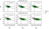 |
Fig. 9. Marginalised posterior distributions in the Ωm − σ8 plane, with 68% and 95% confidence intervals, for redshift and photo-z space, using a binwidth of Δz = 0.2 and Δz = 0.4, in the upper and lower panels, respectively. The contours are for w(θ) and Cℓ. The dashed lines indicate the Ωm and σ8 values of the PINOCCHIO simulation, while the dot-dashed line shows the predicted S8 degeneracy curve. |
6.2. Results
In this section we present the results of the cosmological analyses of ξ(s), w(θ) and Cℓ. We sampled the posterior distribution with a Monte carlo Markov chain (MCMC), assuming different redshift bins as statistically independent. For all the probes considered, the cosmological parameters of the simulations, corresponding to Planck Collaboration XVI (2014), are correctly recovered, falling within the range at 95% of the corner plot in the Ωm − σ8 plane. Systematic effects causing a slight shift of the marginalised posterior distribution can rise due to non-linearities or to the inaccuracy of the halo bias model. The theoretical prediction provided by Tinker et al. (2010) overestimates the numerical bias by about 5%, for low masses and redshifts, see Fig. 2 in Euclid Collaboration (2021). On the other hand, at high masses and redshifts, there is an underestimation of about 10%. However, these scales are excluded from the redshift cut of our sample.
In Fig. 9 we summarise the result of the angular tomographic analysis. First, we note that w(θ) and Cℓ produce largely overlapping results, giving us the same cosmological information. This is due to the fact that our catalogue has a large coverage of the sky, allowing us to investigate a wide range of different wavelengths. The relative shift of their posteriors, for example, for Δz = 0.2 and σz = 0.02(1 + z) or Δz = 0.4 and σz = 0.05(1 + z), can be interpreted as an effect of the variance of the specific PLC, and it is not found when instead of measuring on a single mock we consider the average measure from the full set of 1000 PINOCCHIO simulations.
Second, by widening the binwidth from Δz = 0.2 to Δz = 0.4, the marginalised posterior distributions of w(θ) and Cℓ suffer a broadening on both Ωm and σ8. For example, the constraints from the angular correlation function slightly change from  to
to  , and from
  to
to  , respectively. With a binwidth of Δz = 0.4 we have both more statistics and less shot noise, as we include a larger number of dark matter haloes. However, the effective bias is considered as a constant, within a given redshift bin, to be taken out of the integrals in Eqs. (32) and (46). This may have systematic consequences for the parameters estimation. Furthermore, the 2D clustering is modified by projection effects that aggregate structures that are not physically bound. In addition, the deeper radial projection erases the BAO peak, because its physical size ends up in a wider range of angular scales. This highlights the importance of defining an appropriate tomographic strategy in clustering studies.
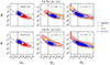 |
Fig. 10. Marginalised posterior distributions in the Ωm − σ8 plane, with 68% and 95% confidence intervals, for redshift and photo-z space, using a binwidth of Δz = 0.2 and Δz = 0.4, in the upper and lower panels, respectively. The contours are for the different multipoles of ξ(s). The dashed lines indicate the Ωm and σ8 values of the PINOCCHIO simulation, while the dot-dashed line shows the predicted S8 degeneracy curve. |
The introduction of photo-z errors, on the other hand, determines a general reduction of the clustering signal, resulting in a loss of constraining power. The posterior distributions given by w(θ) broaden from  to
to  , and from
  to
to  , if Δz = 0.2, while they widen from
  to
to  , and from
  to
to  , if Δz = 0.4, respectively. These results show us that the constraints on σ8 are generally more stable than the ones on Ωm.
As we can see in Table 1, we have also included some extra shot noise terms for the angular power spectrum. While in general we have verified that these shot noise parameters are characterised by a flat zero mean posterior, we notice that the Ωm − σ8 corner plots, obtained by including these additional free parameters, are slightly wider and better centred.
In Fig. 10 we can see the posterior distributions derived from the 3D correlation function. As in many studies based on real observations, we start from the analysis of the monopole, since it is more stable and less sensitive to the purity of the cluster sample. Then, we progressively take into account the contribution of the quadrupole and the hexadecapole. Focusing on ξ0(s), we found that enlarging the redshift shell from Δz = 0.2 to Δz = 0.4 does not change significantly the redshift-space marginalised distribution, with a maximum shift of 0.01 in the standard deviations of both Ωm and σ8. This result should be interpreted with the fact that in the 3D correlation function the redshift information is not integrated out, thus it contributes to the clustering signal, with only a minor degradation due to the assumption of a constant effective bias in each tomographic bin.
On the other hand, we note that ξ0(s), in contrast to w(θ) and Cℓ, exhibits a significant widening of the confidence intervals as the photo-z errors increase. While, from the point of view of the model, the damping of the power spectrum in Eq. (24) is fully equivalent to the introduction of Gaussian errors in the dN/dz, as shown in Hütsi (2010), it is the measurement that is mainly altered, since the photo-z errors significantly modify the radial component of the clustering, leaving the angular part unaffected. For example, while the 3D correlation function suffers from the complete erosion of the BAO peak, this is still visible in w(θ), which only experiences a reduction in the signal due to differences in the radial distribution within a given photometric redshift interval (see Fig. 5). A second consequence is that, in photo-z space, the parameter ΣNL is not constrained, due to the smearing that affects the BAO peak. Therefore, it behaves as a merely computational expensive complication of the model.
Furthermore, the constraints are better centred on the true cosmology of the simulation as the photo-z errors increase. This is because we start from the assumption of a linear model for P(k), with an infrared (IR) resummation at the BAO peak. As we can see in Fig. 1, this approximation does not hold at low redshift and small scales, because of deviations due to the FoG effect and the non-linear coupling between velocity and density fields (see e.g. Taruya et al. 2010). This could result in a systematic on the estimate of cosmological parameters. Conversely in photo-z space, the effect of non-linearities is diluted by the redshift perturbation, in a similar way to the redshift projection of 2D clustering. This makes it possible to still consider a simple linear power spectrum, avoiding complications in the modelling of the clustering signal.
As evident from Fig. 10, the inclusion of multipoles leads, in general, to a shrinking of the contours along the  degeneration line. We should notice, in particular, that in redshift space the clustering signal comes from the monopole and the quadrupole only, while the contribution of the hexadecapole is negligible, as we can see in Fig. 1, being consistent with zero for s > 20 Mpc h−1 in every bin of our analysis. On the other hand, in photo-z space, the inclusion of ξ2(s) and ξ4(s) is relevant. By way of example, for Δz = 0.4, the constraints on Ωm and σ8 change from
  and
and  , to
, to  and
and  , and finally to
  and
and  , as we add the even multipoles.
In Fig. 11, in order to summarise the cosmological results and to understand what contribution cluster clustering can make, we focus on the structure growth parameter, S8. It is particularly relevant in cosmology, since various measurements in the local Universe (e.g. cosmic shear, galaxy clustering, galaxy and galaxy cluster number counts) have shown a 2 − 3σ tension with the high-z value inferred by studying the CMB anisotropies from Planck (see e.g. Bocquet et al. 2019; Asgari et al. 2021; Heymans et al. 2021; Abbott et al. 2022; Amon et al. 2022), which represents a potential stress for the current ΛCDM model.
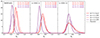 |
Fig. 11. Summary plot for the parameter S8, in redshift and photo-z space with σz = 0.02(1 + z) and σz = 0.05(1 + z), panels from left to right, for w(θ) and ξ0(s). The solid lines refer to Δz = 0.2, the dashed lines to Δz = 0.4. The dot-dashed line indicates the S8 value of the PINOCCHIO simulation. |
For the sake of simplicity, we compare only the two-point correlation function in both its variants (i.e. w(θ) and ξ(s)). These two probes lie in configuration space. Moreover, they are built from the same random catalogue, and therefore are subject to common systematics. While in redshift space their competitiveness essentially depends on the width of the analysed redshift bins, with a slight decentring of ξ0(s) due to non-linearities at small scales, we note that in the presence of a large photo-z errors, such as 0.05(1 + z), w(θ) is always favoured over ξ0(s), with  versus
  and
and  , versus
  , for Δz = 0.2 and Δz = 0.4, respectively. The latter requires the inclusion of the multipoles to produce results comparable or superior to the 2D clustering, depending on Δz. In this case, more care should be taken to avoid systematics due to non-linearities not included in the model, at scales s < 20 Mpc h−1. The intermediate case, with σz = 0.02(1 + z), shows that the 2D correlation function is clearly preferred for Δz = 0.2, while it is slightly disfavoured for Δz = 0.4, due to the lack of the redshift information. This fact confirms the possible advantages and the competitiveness of the angular tomographic clustering within photometric redshift surveys. In particular, the potential and limitations of this approach have already been tested in the angular clustering analysis of the KiDS-DR3 cluster catalogue, discussed in Romanello et al. (2024), where the constraint on S8 are mildly more stringent than the corresponding 3D study (Lesci et al. 2022b).
7. Conclusions
In this paper we analysed the clustering properties of dark matter haloes from the PINOCCHIO simulation in preparation for subsequent work to be carried out on forthcoming galaxy cluster catalogues from Stage III and Stage IV photometric surveys. We used a PLC with an angular size of 60 deg, thus covering a circular area of 10 313 deg2, namely one-quarter of the sky. We selected dark matter haloes with a virial mass greater than 1014 M⊙ h−1 and redshift in the range 0.2 < z < 1.0. The mass selection reproduces to a good approximation what is expected for future cluster catalogues identified in the Stage IV photometric surveys, while the selection in z excludes the low-redshift regime, where it will be difficult to perform a robust lensing analysis for the mass calibration of real galaxy clusters, and the high-redshift regime, where the clustering signal is completely dominated by shot noise.
Our study used a tomographic approach adopting the binwidths Δz = 0.2 − 0.4 (i.e. four or two redshift bins) to compare 3D and 2D clustering. The former was analysed by means of the 3D two-point correlation function, while for the latter we made use of the angular correlation function and its spherical harmonic counterpart, the angular power spectrum. For each cosmological probe, we estimated the numerical covariance matrix from a set of 1000 mock catalogues, in both redshift space and photo-z space. For this purpose we introduced Gaussian errors on the halo redshifts, with zero mean and standard deviation given by σz = σz, 0(1 + z), with the typical σz, 0 of photometric redshift surveys, namely 0.02 and 0.05.
We used a linear model for the power spectrum, including the IR-resummation, which characterises non-linear damping phenomena at the BAO scale. The 3D correlation function was obtained via Fourier transform of the corresponding P(k), computing the effective bias of dark matter haloes by assuming the model presented in Tinker et al. (2010) for the halo bias, and the parametrisation of Despali et al. (2016) for the halo mass function. The angular correlation function and power spectrum are modelled from the radial projection of the corresponding 3D correlation function and power spectrum, respectively, with a selection kernel that takes into account the normalised redshift distribution of haloes. RSDs are modelled in the Kaiser limit for the correlation functions, while they are not considered in the Cℓ as they only slightly affect the largest angular scales, being fully subdominant relative to the measurement uncertainties. We found that they have only a minor effect on ξ0(s) and on w(θ), quantified in a boost factor of 1.1 - 1.2, due to the high bias of the tracers. On the other hand, photo-z errors play the major role in suppressing the clustering signal and the numerical errors. In particular, they modify the small-scale slope of the 3D correlation function monopole, and completely erase the BAO features, which conversely remain visible in w(θ). Moreover, photo-z errors determine a substantial increase in the contribution of the quadrupole and the hexadecapole. In particular, ξ2(s) changes its sign, moving from redshift space to photo-z space, while ξ4(s), which is consistent with zero in redshift space, becomes dominant for σz ≳ 0.02(1 + z). For the angular power spectrum, we verified that the Limber approximation and the Poissonian assumption for the shot noise hold over the full redshift interval and angular scales considered in our analysis.
Finally, we performed a Bayesian MCMC analysis to constrain fundamental cosmological parameters, such as Ωm and σ8. Even though all cosmological probes are able to accurately estimate the cosmological parameters of the simulations, we find that the posterior distributions obtained from the 3D correlation function degrade more in the presence of photo-z errors than from its angular counterparts. In the presence of large photo-z errors, ξ0(s) produces wider constraints on the structure growth parameter, S8, with respect to w(θ). Conversely, by also exploiting the redshift infomation, it is less affected by the specific tomographic redshift binning strategy adopted, but is more sensitive to non-linearities that characterise the small-scale clustering. The inclusion of the two-point correlation function multipoles determines a collapse of the Ωm − σ8 contours along the S8 degeneracy curve, which is more relevant in photo-z space, while the contribution of ξ4(s) is negligible in redshift space.
On the other hand, w(θ) and Cℓ provide the same cosmological information, and unbiased cosmological constraints, which in turn complement that obtained from the 3D analysis, with the advantage of being able to rely on a linear model for P(k) since non-linearities are diluted by projection effects. Moreover, in the presence of photo-z errors, for σz, 0 ≳ 0.02, the angular clustering shows its full potential as a cosmological probe, with respect to the traditional 3D study, with the advantage of not requiring a fiducial cosmology to convert redshifts into distances in the measurements. This comparison was already performed in Romanello et al. (2024), where we successfully applied the models developed in this paper to the AMICO KiDS-DR3 galaxy cluster catalogue, finding consistent results with respect to the ξ0(s) analysis, with slightly more stringent constraints on S8. This highlights the significance of extending the analysis of 2D clustering to other cosmological parameters, for example studying the degeneracy in the w0 − wa dynamical dark energy plane and the galaxy cluster catalogues that will be available from ongoing Stage III and Stage IV photometric surveys, such as the forthcoming data releases of KiDS and Euclid.
Acknowledgments
We acknowledge the financial contribution from the grant PRIN-MUR 2022 20227RNLY3 “The concordance cosmological model: stress-tests with galaxy clusters” supported by Next Generation EU and from the grants ASI n.2018-23-HH.0 and n. 2024-10-HH.0 “Attivitá scientifiche per la missione Euclid – fase E”, and the use of computational resources from the parallel computing cluster of the Open Physics Hub (https://site.unibo.it/openphysicshub/en) at the Physics and Astronomy Department in Bologna. We would like to thank P. Monaco for the production of the PINOCCHIO mocks, R. Zangarelli and the anonymous referee for the constructive suggestions that improved this work.
References
- Abbott, T. M. C., Aguena, M., Alarcon, A., et al. 2022, Phys. Rev. D, 105, 023520 [CrossRef] [Google Scholar]
- Aihara, H., Arimoto, N., Armstrong, R., et al. 2018, PASJ, 70, S4 [NASA ADS] [Google Scholar]
- Alcock, C., & Paczynski, B. 1979, Nature, 281, 358 [NASA ADS] [CrossRef] [Google Scholar]
- Allen, S. W., Evrard, A. E., & Mantz, A. B. 2011, ARA&A, 49, 409 [Google Scholar]
- Alonso, D., Sanchez, J., Slosar, A., & LSST Dark Energy Science Collaboration 2019, MNRAS, 484, 4127 [NASA ADS] [CrossRef] [Google Scholar]
- Amon, A., Gruen, D., Troxel, M. A., et al. 2022, Phys. Rev. D, 105, 023514 [NASA ADS] [CrossRef] [Google Scholar]
- Ando, S., Benoit-Lévy, A., & Komatsu, E. 2018, MNRAS, 473, 4318 [NASA ADS] [CrossRef] [Google Scholar]
- Asgari, M., Lin, C.-A., Joachimi, B., et al. 2021, A&A, 645, A104 [NASA ADS] [CrossRef] [EDP Sciences] [Google Scholar]
- Asorey, J., Crocce, M., Gaztañaga, E., & Lewis, A. 2012, MNRAS, 427, 1891 [CrossRef] [Google Scholar]
- Ata, M., Baumgarten, F., Bautista, J., et al. 2018, MNRAS, 473, 4773 [NASA ADS] [CrossRef] [Google Scholar]
- Avila, S., Crocce, M., Ross, A. J., et al. 2018, MNRAS, 479, 94 [NASA ADS] [CrossRef] [Google Scholar]
- Balaguera-Antolínez, A., Bilicki, M., Branchini, E., & Postiglione, A. 2018, MNRAS, 476, 1050 [Google Scholar]
- Baldauf, T., Seljak, U., Smith, R. E., Hamaus, N., & Desjacques, V. 2013, Phys. Rev. D, 88, 083507 [NASA ADS] [CrossRef] [Google Scholar]
- Bardeen, J. M., Bond, J. R., Kaiser, N., & Szalay, A. S. 1986, ApJ, 304, 15 [Google Scholar]
- Bellagamba, F., Sereno, M., Roncarelli, M., et al. 2019, MNRAS, 484, 1598 [Google Scholar]
- Beutler, F., Saito, S., Seo, H.-J., et al. 2014, MNRAS, 443, 1065 [NASA ADS] [CrossRef] [Google Scholar]
- Blake, C., & Bridle, S. 2005, MNRAS, 363, 1329 [Google Scholar]
- Blake, C., Collister, A., Bridle, S., & Lahav, O. 2007, MNRAS, 374, 1527 [NASA ADS] [CrossRef] [Google Scholar]
- Bocquet, S., Dietrich, J. P., Schrabback, T., et al. 2019, ApJ, 878, 55 [Google Scholar]
- Bond, J. R., Cole, S., Efstathiou, G., & Kaiser, N. 1991, ApJ, 379, 440 [NASA ADS] [CrossRef] [Google Scholar]
- Branchini, E., Camera, S., Cuoco, A., et al. 2017, ApJS, 228, 8 [Google Scholar]
- Budavári, T., Connolly, A. J., Szalay, A. S., et al. 2003, ApJ, 595, 59 [CrossRef] [Google Scholar]
- Cabré, A., Fosalba, P., Gaztañaga, E., & Manera, M. 2007, MNRAS, 381, 1347 [CrossRef] [Google Scholar]
- Camacho, H., Kokron, N., Andrade-Oliveira, F., et al. 2019, MNRAS, 487, 3870 [NASA ADS] [CrossRef] [Google Scholar]
- Camera, S., Fonseca, J., Maartens, R., & Santos, M. G. 2018, MNRAS, 481, 1251 [CrossRef] [Google Scholar]
- Chan, K. C., Crocce, M., Ross, A. J., et al. 2018, MNRAS, 480, 3031 [NASA ADS] [CrossRef] [Google Scholar]
- Chan, K. C., Ferrero, I., Avila, S., et al. 2022, MNRAS, 511, 3965 [NASA ADS] [CrossRef] [Google Scholar]
- Costanzi, M., Sartoris, B., Xia, J.-Q., et al. 2013, JCAP, 2013, 020 [CrossRef] [Google Scholar]
- Crocce, M., Cabré, A., & Gaztañaga, E. 2011, MNRAS, 414, 329 [NASA ADS] [CrossRef] [Google Scholar]
- Dark Energy Survey Collaboration (Abbott, T., et al.) 2016, MNRAS, 460, 1270 [Google Scholar]
- de Jong, J. T. A., Verdoes Kleijn, G. A., Erben, T., et al. 2017, A&A, 604, A134 [NASA ADS] [CrossRef] [EDP Sciences] [Google Scholar]
- Despali, G., Giocoli, C., Angulo, R. E., et al. 2016, MNRAS, 456, 2486 [NASA ADS] [CrossRef] [Google Scholar]
- Dodelson, S. 2003, Modern Cosmology (Amsterdam: Academic Press) [Google Scholar]
- Eisenstein, D. J., & Hu, W. 1998, ApJ, 496, 605 [Google Scholar]
- Euclid Collaboration (Adam, R., et al.) 2019, A&A, 627, A23 [NASA ADS] [CrossRef] [EDP Sciences] [Google Scholar]
- Euclid Collaboration (Blanchard, A., et al.) 2020, A&A, 642, A191 [NASA ADS] [CrossRef] [EDP Sciences] [Google Scholar]
- Euclid Collaboration (Fumagalli, A., et al.) 2021, A&A, 652, A21 [NASA ADS] [CrossRef] [EDP Sciences] [Google Scholar]
- Euclid Collaboration (Keihänen, E., et al.) 2022a, A&A, 666, A129 [CrossRef] [EDP Sciences] [Google Scholar]
- Euclid Collaboration (Scaramella, R., et al.) 2022b, A&A, 662, A112 [NASA ADS] [CrossRef] [EDP Sciences] [Google Scholar]
- Euclid Collaboration (Fumagalli, A., et al.) 2024a, A&A, 683, A253 [NASA ADS] [CrossRef] [EDP Sciences] [Google Scholar]
- Euclid Collaboration (Lesci, G. F., et al.) 2024b, A&A, 684, A139 [NASA ADS] [CrossRef] [EDP Sciences] [Google Scholar]
- Euclid Collaboration (Mellier, Y., et al.) 2025, A&A, in press https://doi.org/10.1051/0004-6361/202450810 [Google Scholar]
- Fumagalli, A., Biagetti, M., Saro, A., et al. 2022, JCAP, 2022, 022 [CrossRef] [Google Scholar]
- Fumagalli, A., Costanzi, M., Saro, A., Castro, T., & Borgani, S. 2024, A&A, 682, A148 [NASA ADS] [CrossRef] [EDP Sciences] [Google Scholar]
- Gao, L., Springel, V., & White, S. D. M. 2005, MNRAS, 363, L66 [NASA ADS] [CrossRef] [Google Scholar]
- Garaldi, E., Nori, M., & Baldi, M. 2020, MNRAS, 499, 2685 [CrossRef] [Google Scholar]
- García-Farieta, J. E., Marulli, F., Moscardini, L., Veropalumbo, A., & Casas-Miranda, R. A. 2020, MNRAS, 494, 1658 [CrossRef] [Google Scholar]
- Ghirardini, V., Bulbul, E., Artis, E., et al. 2024, A&A, 689, A298 [NASA ADS] [CrossRef] [EDP Sciences] [Google Scholar]
- Giocoli, C., Bartelmann, M., Sheth, R. K., & Cacciato, M. 2010, MNRAS, 408, 300 [NASA ADS] [CrossRef] [Google Scholar]
- Giocoli, C., Di Meo, S., Meneghetti, M., et al. 2017, MNRAS, 470, 3574 [NASA ADS] [CrossRef] [Google Scholar]
- Giocoli, C., Monaco, P., Moscardini, L., et al. 2020, MNRAS, 496, 1307 [CrossRef] [Google Scholar]
- Giocoli, C., Marulli, F., Moscardini, L., et al. 2021, A&A, 653, A19 [NASA ADS] [CrossRef] [EDP Sciences] [Google Scholar]
- Giocoli, C., Palmucci, L., Lesci, G. F., et al. 2024, A&A, 687, A79 [NASA ADS] [CrossRef] [EDP Sciences] [Google Scholar]
- Górski, K. M., Hivon, E., Banday, A. J., et al. 2005, ApJ, 622, 759 [Google Scholar]
- Hamilton, A. J. S. 1992, ApJ, 385, L5 [NASA ADS] [CrossRef] [Google Scholar]
- Hauser, M. G., & Peebles, P. J. E. 1973, ApJ, 185, 757 [NASA ADS] [CrossRef] [Google Scholar]
- Hernández-Aguayo, C., Springel, V., Pakmor, R., et al. 2023, MNRAS, 524, 2556 [CrossRef] [Google Scholar]
- Heymans, C., Tröster, T., Asgari, M., et al. 2021, A&A, 646, A140 [NASA ADS] [CrossRef] [EDP Sciences] [Google Scholar]
- Hildebrandt, H., Viola, M., Heymans, C., et al. 2017, MNRAS, 465, 1454 [Google Scholar]
- Hütsi, G. 2010, MNRAS, 401, 2477 [CrossRef] [Google Scholar]
- Hütsi, G., Gilfanov, M., Kolodzig, A., & Sunyaev, R. 2014, A&A, 572, A28 [NASA ADS] [CrossRef] [EDP Sciences] [Google Scholar]
- Ibitoye, A., Tramonte, D., Ma, Y.-Z., & Dai, W.-M. 2022, ApJ, 935, 18 [NASA ADS] [CrossRef] [Google Scholar]
- Jackson, J. C. 1972, MNRAS, 156, 1P [CrossRef] [Google Scholar]
- Kaiser, N. 1984, ApJ, 284, L9 [NASA ADS] [CrossRef] [Google Scholar]
- Kuijken, K., Heymans, C., Dvornik, A., et al. 2019, A&A, 625, A2 [NASA ADS] [CrossRef] [EDP Sciences] [Google Scholar]
- Landy, S. D., & Szalay, A. S. 1993, ApJ, 412, 64 [Google Scholar]
- Laureijs, R., Amiaux, J., Arduini, S., et al. 2011, arXiv e-prints [arXiv:1110.3193] [Google Scholar]
- Lesci, G. F., Marulli, F., Moscardini, L., et al. 2022a, A&A, 659, A88 [NASA ADS] [CrossRef] [EDP Sciences] [Google Scholar]
- Lesci, G. F., Nanni, L., Marulli, F., et al. 2022b, A&A, 665, A100 [NASA ADS] [CrossRef] [EDP Sciences] [Google Scholar]
- Lewis, A., Challinor, A., & Lasenby, A. 2000, ApJ, 538, 473 [Google Scholar]
- Limber, D. N. 1953, ApJ, 117, 134 [NASA ADS] [CrossRef] [Google Scholar]
- Lindholm, V., Finoguenov, A., Comparat, J., et al. 2021, A&A, 646, A8 [NASA ADS] [CrossRef] [EDP Sciences] [Google Scholar]
- Loureiro, A., Moraes, B., Abdalla, F. B., et al. 2019, MNRAS, 485, 326 [NASA ADS] [CrossRef] [Google Scholar]
- Makiya, R., Ando, S., & Komatsu, E. 2018, MNRAS, 480, 3928 [Google Scholar]
- Mandelbaum, R., Slosar, A., Baldauf, T., et al. 2013, MNRAS, 432, 1544 [NASA ADS] [CrossRef] [Google Scholar]
- Manera, M., & Gaztañaga, E. 2011, MNRAS, 415, 383 [NASA ADS] [CrossRef] [Google Scholar]
- Manera, M., Scoccimarro, R., Percival, W. J., et al. 2013, MNRAS, 428, 1036 [Google Scholar]
- Marulli, F., Baldi, M., & Moscardini, L. 2012, MNRAS, 420, 2377 [NASA ADS] [CrossRef] [Google Scholar]
- Marulli, F., Veropalumbo, A., & Moresco, M. 2016, Astronomy and Computing, 14, 35 [NASA ADS] [CrossRef] [Google Scholar]
- Marulli, F., Veropalumbo, A., Sereno, M., et al. 2018, A&A, 620, A1 [NASA ADS] [CrossRef] [EDP Sciences] [Google Scholar]
- Marulli, F., Veropalumbo, A., García-Farieta, J. E., et al. 2021, ApJ, 920, 13 [Google Scholar]
- Maturi, M., Bellagamba, F., Radovich, M., et al. 2019, MNRAS, 485, 498 [Google Scholar]
- McClintock, T., Varga, T. N., Gruen, D., et al. 2019, MNRAS, 482, 1352 [Google Scholar]
- McNamara, B. R., & Nulsen, P. E. J. 2007, ARA&A, 45, 117 [NASA ADS] [CrossRef] [Google Scholar]
- Mo, H. J., & White, S. D. M. 1996, MNRAS, 282, 347 [Google Scholar]
- Monaco, P. 2016, Galaxies, 4, 53 [NASA ADS] [CrossRef] [Google Scholar]
- Monaco, P., Theuns, T., & Taffoni, G. 2002, MNRAS, 331, 587 [Google Scholar]
- Monaco, P., Sefusatti, E., Borgani, S., et al. 2013, MNRAS, 433, 2389 [NASA ADS] [CrossRef] [Google Scholar]
- Moscardini, L., Matarrese, S., & Mo, H. J. 2001, MNRAS, 327, 422 [NASA ADS] [CrossRef] [Google Scholar]
- Munari, E., Monaco, P., Sefusatti, E., et al. 2017, MNRAS, 465, 4658 [Google Scholar]
- Norberg, P., Baugh, C. M., Gaztañaga, E., & Croton, D. J. 2009, MNRAS, 396, 19 [Google Scholar]
- Padmanabhan, N., Schlegel, D. J., Seljak, U., et al. 2007, MNRAS, 378, 852 [NASA ADS] [CrossRef] [Google Scholar]
- Paech, K., Hamaus, N., Hoyle, B., et al. 2017, MNRAS, 470, 2566 [NASA ADS] [CrossRef] [Google Scholar]
- Park, Y., Sunayama, T., Takada, M., et al. 2023, MNRAS, 518, 5171 [Google Scholar]
- Peacock, J. A., Cole, S., Norberg, P., et al. 2001, Nature, 410, 169 [Google Scholar]
- Peebles, P. J. E. 1973, ApJ, 185, 413 [Google Scholar]
- Pezzotta, A., de la Torre, S., Bel, J., et al. 2017, A&A, 604, A33 [NASA ADS] [CrossRef] [EDP Sciences] [Google Scholar]
- Planck Collaboration XVI. 2014, A&A, 571, A16 [NASA ADS] [CrossRef] [EDP Sciences] [Google Scholar]
- Press, W. H., & Schechter, P. 1974, ApJ, 187, 425 [Google Scholar]
- Romanello, M., Marulli, F., Moscardini, L., et al. 2024, A&A, 682, A72 [NASA ADS] [CrossRef] [EDP Sciences] [Google Scholar]
- Ross, A. J., Percival, W. J., Crocce, M., Cabré, A., & Gaztañaga, E. 2011, MNRAS, 415, 2193 [NASA ADS] [CrossRef] [Google Scholar]
- Rykoff, E. S., Rozo, E., Busha, M. T., et al. 2014, ApJ, 785, 104 [Google Scholar]
- Salazar-Albornoz, S., Sánchez, A. G., Padilla, N. D., & Baugh, C. M. 2014, MNRAS, 443, 3612 [NASA ADS] [CrossRef] [Google Scholar]
- Salazar-Albornoz, S., Sánchez, A. G., Grieb, J. N., et al. 2017, MNRAS, 468, 2938 [NASA ADS] [CrossRef] [Google Scholar]
- Sánchez, A. G., Grieb, J. N., Salazar-Albornoz, S., et al. 2017, MNRAS, 464, 1493 [CrossRef] [Google Scholar]
- Sartoris, B., Biviano, A., Fedeli, C., et al. 2016, MNRAS, 459, 1764 [Google Scholar]
- Sereno, M., Veropalumbo, A., Marulli, F., et al. 2015, MNRAS, 449, 4147 [NASA ADS] [CrossRef] [Google Scholar]
- Sheth, R. K., Mo, H. J., & Tormen, G. 2001, MNRAS, 323, 1 [NASA ADS] [CrossRef] [Google Scholar]
- Springel, V. 2005, MNRAS, 364, 1105 [Google Scholar]
- Springel, V., Yoshida, N., & White, S. D. M. 2001, New Astron., 6, 79 [Google Scholar]
- Springel, V., Pakmor, R., Pillepich, A., et al. 2018, MNRAS, 475, 676 [Google Scholar]
- Sunayama, T. 2023, MNRAS, 521, 5064 [NASA ADS] [CrossRef] [Google Scholar]
- Taruya, A., Nishimichi, T., & Saito, S. 2010, Phys. Rev. D, 82, 063522 [NASA ADS] [CrossRef] [Google Scholar]
- Thomas, S. A., Abdalla, F. B., & Lahav, O. 2011, MNRAS, 412, 1669 [NASA ADS] [CrossRef] [Google Scholar]
- Tinker, J. L., Robertson, B. E., Kravtsov, A. V., et al. 2010, ApJ, 724, 878 [NASA ADS] [CrossRef] [Google Scholar]
- To, C., Krause, E., Rozo, E., et al. 2021, Phys. Rev. Lett., 126, 141301P [CrossRef] [Google Scholar]
- Tormen, G. 1998, MNRAS, 297, 648 [NASA ADS] [CrossRef] [Google Scholar]
- Veropalumbo, A., Marulli, F., Moscardini, L., Moresco, M., & Cimatti, A. 2014, MNRAS, 442, 3275 [NASA ADS] [CrossRef] [Google Scholar]
- Veropalumbo, A., Marulli, F., Moscardini, L., Moresco, M., & Cimatti, A. 2016, MNRAS, 458, 1909 [NASA ADS] [CrossRef] [Google Scholar]
- Vogelsberger, M., Marinacci, F., Torrey, P., & Puchwein, E. 2020, Nature Reviews Physics, 2, 42 [CrossRef] [Google Scholar]
- Voit, G. M. 2005, Reviews of Modern Physics, 77, 207 [NASA ADS] [CrossRef] [Google Scholar]
- Wright, A. H., Kuijken, K., Hildebrandt, H., et al. 2024, A&A, 686, A170 [NASA ADS] [CrossRef] [EDP Sciences] [Google Scholar]
- Zu, Y., Mandelbaum, R., Simet, M., Rozo, E., & Rykoff, E. S. 2017, MNRAS, 470, 551 [CrossRef] [Google Scholar]
Appendix A: Reducing the sky coverage
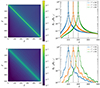 |
Fig. A.1. Mixing matrices for different sky coverages. Left panels: Colour plots of the mixing matrix, Rℓℓ′, computed up to ℓ = 500 with the public code NAMASTER (Alonso et al. 2019). Right panels: Plots of Rℓℓ*/Rℓ*ℓ*, centred in three different multipoles, at ℓ = 100 (blue), 150 (orange) and 200 (green). They quantify the mode-mode coupling related to the partial sky coverage, reflecting the blurring of the mixing matrix along the diagonal. The grey shaded regions indicate the multipole range of Δℓ in which we bin our measurements. The top panels are computed from the 10313 deg2 region covered by the full PINOCCHIO footprint mask, while at the bottom we focus on the 1004 deg2 subregion. |
In partial-sky surveys, spherical harmonics no longer provide a complete orthonormal basis for the expansion of the angular overdensities (Camacho et al. 2019). The masked density field is related to its full-sky counterpart through a binary mask function,  , which can be considered as an angular window function. Its effect propagates into the power spectrum evaluation, in the form of a coupling between different multipoles, which becomes progressively more important for lower sky coverages and survey fragmentation. In particular, the measured power spectrum at multipole ℓ depends on an underlying range of multipoles ℓ′ (Blake et al. 2007). The power transfer between different multipoles is described by the mixing matrix, Rℓℓ′, which depends only on the geometry of the angular mask. It reduces to the identity matrix in full-sky surveys and can be expressed in terms of the Wigner 3j symbols
 (A.1)
(A.1)
where
 (A.2)
(A.2)
Here Iℓm represents the spherical harmonic coefficient of the mask, which can be approximated in a pixelated sky as
 (A.3)
(A.3)
With the mixing matrix we can link the ensemble average of the measured power spectrum with the theoretical power spectrum through (Balaguera-Antolínez et al. 2018)
 (A.4)
(A.4)
We estimate the mixing matrix of the footprint masks using the publicly available code NAMASTER6 (Alonso et al. 2019), which provides a general framework for the pseudo-Cℓ analysis.
To better reproduce the observational conditions of photometric surveys, which often scan separated parts of the sky, we produced an angular mask composed of three different patches, two near the equator (P1 and P2), and another further south, (P3). Their angular limits are given respectively by
-
P1: RA ∈[−60, −30], Dec ∈[−10, 0];
-
P2: RA ∈[0, 30], Dec ∈[4, 10];
-
P3: RA ∈[−30, 30], Dec ∈[−40, −30].
The final effective area is equal to 1004 deg2, which simulates the expected sky coverage of the cluster catalogue of KiDS-DR4, for which we plan to carry out a subsequent in-depth study.
Reducing the sky coverage has important consequences on our analysis. First, it increases the angular auto-correlation, with a blurring of the correlation matrix both in configuration and in spherical harmonic space. At the level of the angular power spectrum, we find that the mixing matrix calculated over an area of 1004 deg2 is more blurred than the one computed over the full PLC, as we can see in Fig. A.1, with the convolution function Rℓ*ℓ′. The grey shaded regions highlight the Δℓ = 8 bandwidth, which allows us to include almost all of the clustering signal, reducing the power transfer between different ℓ bands due to the off-diagonal terms, while with the reduced sky coverage, the same band of Δℓ = 8 identifies only 50% of the transferred power.
Reducing the survey area, on the other hand, does not change the shot noise, since both Ωsky and Nh decrease in the same way. However, a smaller range of wavelengths can be investigated within the reduced volume. This fact suggests that it is possible to exploit Cℓ and w(θ) as complementary sources of cosmological information and specifically, to use their comparison to assess possible model systematics.
Appendix B: Analytical modelling of the covariance matrix
A fundamental aspect of cluster clustering cosmology is the correct evaluation of measurement errors. Biases in the determination of cosmological parameters can be present, if all significant observational systematic uncertainties are not properly taken into account.
The estimation of covariance matrices, which summarise the set of uncertainties associated with the observables, is therefore a fundamental challenge for the future. Analytical covariance matrix calculations are probably the best solution, as they do not require large computational resources. In addition, they are noise-free and naturally include the dependence on cosmological parameters (Euclid Collaboration 2024a). However, the accuracy of analytical models might be limited due to the complex physics of structure formation, which introduces non-linearities and non-Gaussianities in clustering, and by the necessity of appropriate models for shot noise and RSDs (Manera et al. 2013; Euclid Collaboration 2024a). These and other observational effects, such as angular masks and redshift uncertainties, can lead to systematic theoretical errors, and therefore their modelling needs to be validated against simulations in any case (Avila et al. 2018; Fumagalli et al. 2022; Euclid Collaboration 2024a).
In this section we test some simple theoretical models for the covariance matrix of the angular two-point correlation function and power spectrum. The validation of semi-analytic models for the covariance of the 2D clustering is beyond the scope of this paper, while for the 3D two-point correlation function we rely on the results presented in the works by Fumagalli et al. (2022), Euclid Collaboration (2024a).
B.1. Covariance matrix of Cℓ
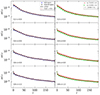 |
Fig. B.1. Errors in the angular power spectrum, derived as the square root of diagonal elements of Covℓℓ′, in real (blue squares), redshift (with σz = 0, black circles) and in photo-z space, with σz = 0.02, (red triangles) and σz = 0.05 (green triangles), from the numerical covariance matrix measured from 1000 mocks. The lines show the results obtained with the linear power spectrum in the Limber approximation (solid black line), with the exact integration given by Eq. (43), which also includes the modelling of the RSDs (dashed red line) and with the damped linear power spectrum in the Limber approximation (solid red and green lines). |
Concerning angular clustering, several works in the literature considered internal subsampling error estimates, such as bootstrap or jackknife (e.g. Paech et al. 2017; Balaguera-Antolínez et al. 2018). These methods are quite accurate for 2D clustering, because the radial projection alleviates the tensions that emerge in the 3D correlation (Norberg et al. 2009), depending on the scales involved, ensuring a good agreement with theoretical models (Crocce et al. 2011).
In the linear regime we can assume a Gaussian distribution for the aℓms. As a consequence of the Gaussian theory, covariance matrices are limited to diagonal terms (Dodelson 2003). This analytical estimation has been used in several works (Blake et al. 2007; Thomas et al. 2011; Balaguera-Antolínez et al. 2018) and can be written as
 (B.1)
(B.1)
where the Kronecker delta, δℓℓ′K, ensures the diagonality of the covariance matrix. It consists of an average over 2ℓ+1 different realisations, one for each m in a given multipole, with the cosmic variance term, Cℓ, and the shot noise term, Ωsky/Nh, that depends on the number of haloes in the selected redshift bin. The partial sky coverage enters in Eq. (B.1) as a boost factor 1/fsky, though the covariance matrix remains diagonal. This is accurate enough because, as we have already discussed, the off-diagonal elements of the correlation matrix become negligible when averaging in the ℓ bands and consequently dividing for their size Δℓ. Equation (B.1) depends on the theoretical power spectrum Cℓ, which includes the modelling of observational effects, such as photo-z errors and RSDs, according to Eqs. (37) and (43), respectively. In Fig. B.1 we show the measured errors, which are obtained as the square root of the diagonal elements of the numerical covariance matrix,  . These are compared with the theory, finding a generally good agreement, within 10%. By looking at Fig. 7, the fact that the numerical errors slightly underestimate the model predictions can be explained as follows. The partial sky coverage of the PLCs determines the emergence of a non-diagonal correlation, spread over an interval of multipoles given approximately by ±1/fsky, as already found by Crocce et al. (2011). Since for our mocks fsky = 0.25, the expected correlation width is Δℓ = 8 and the measured non-diagonal terms rapidly drop to a noise consistent with zero. As discussed in Crocce et al. (2011), the integral of the elements of the covariance matrix arranged along a row gives us
 (B.2)
(B.2)
In full-sky surveys, all the errors are summarised in the diagonal of the covariance matrix. However, the presence of boundaries causes a leakage of the diagonal errors to other ℓ modes, so that their values become lower than the simple fsky boost given by Eq. (B.1). As we have seen in Fig. A.1, thanks to the large sky coverage offered by the PINOCCHIO PLCs, almost all the correlation is concentrated within the band Δℓ. Therefore, the diagonal model in Eq. (B.1) is accurate enough to describe the numerical covariance. For smaller and highly fragmented regions of the sky, the approximation in Eq. (B.1) does not hold. This is clearly visible in Fig. B.2, where we show the result, after repeating the analysis but considering the 1004 deg2 area subsample. Here, the diagonal approximation (black lines) overestimates the numerical errors in all redshift bins, with a more dramatic effect in the analysis of the reduced area. This issue can be resolved by relaxing the assumption of diagonality of the covariance matrix. We can think of the Kronecker delta as the full-sky limit of the mixing matrix, Rℓℓ′. Thus, we can make the mixing matrix block-diagonal and compute the covariance as (Loureiro et al. 2019)
 (B.3)
(B.3)
with the second fsky in the denominator coming up as the normalisation factor of the mixing matrix.
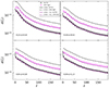 |
Fig. B.2. Comparison between diagonal and non-diagonal errors on the real-space angular power spectrum, Cℓ, in different redshift bins. Grey squares and magenta pentagons are measured from the set of mocks, with the full PLCs sky coverage and with its 1000 deg2 subregions, respectively. The black lines are computed through the Limber approximation, with the diagonal |

Furthermore, as we have already seen in Sect. 5.1, the role of the RSDs is only relevant at the largest angular scales and increases progressively with z. However, for 0.6 < z < 0.8 and 0.8 < z < 1.0, we find a percentage difference in errors between real and redshift space greater than 10% only at ℓ < 10. To account also for non-linearities at the BAO scale, we use the best-fit ΣNL values of Eq. (9), derived by fixing the cosmological parameters at Planck Collaboration XVI (2014), the ones of the PINOCCHIO simulations. However, their role in the Cℓ error estimate is completely negligible, so they are not considered in the plot. As noted by Crocce et al. (2011), the damping of the baryon acoustic features has no effect on the error predictions on the large angular scales.
Analogously to what we found in Sect. 5.1, photo-z uncertainties also determine a suppression in the error estimation, which is modelled by convolving the angular power spectrum model, Cℓ, with the Gaussian distribution in Eq. (1).
B.2. Covariance matrix of w(θ)
The angular correlation function can be derived analytically from Cℓ, by summation over an infinite set of multipoles, sampling progressively smaller angular scales,
 (B.4)
(B.4)
without the shot noise term, since it only contributes to the zero separation limit (Chan et al. 2018), and also propagating systematic effects, such as RSDs and partial sky coverage. The covariance matrix of the angular correlation function is related to the Cℓ covariance through (Cabré et al. 2007; Crocce et al. 2011; Ross et al. 2011)
 (B.5)
(B.5)
where θi and θj indicate the angular bins, while μ = cos θ. This yields
 (B.6)
(B.6)
where we set the shot noise to  to simplify the notation.
As for the power spectrum case, the w(θ) covariance matrix is modified by the fact that measurements are computed over finite angular width bins, which reduces the non-diagonal correlation. A correct estimate requires the bin-averaged Legendre polynomials, defined as (Salazar-Albornoz et al. 2014, 2017; Chan et al. 2018)
 (B.7)
(B.7)
where θ+ = θ + Δθ/2 and θ− = θ − Δθ/2 represent the upper and the lower limits of the bin, while μ+ and μ− are the corresponding cosines. This leads to (Salazar-Albornoz et al. 2014)
 (B.8)
(B.8)
Notably, even the covariance matrix for partial sky coverage follows the inverse of fsky. However, this approximation might break when measuring w(θ) in highly fragmented survey areas, where the number of pairs as a function of separation does not simply scale with the effective area, Ωsky, and thus it cannot be reproduced by the shot noise term, Ωsky/Nh (Chan et al. 2018).
Moreover, since the shot noise does not depend on the multipole ℓ, we can make the binomial square explicit, and take  out from the summation. In particular, we can exploit the relation
 (B.9)
(B.9)
obtaining (Chan et al. 2018)
 (B.10)
where the Kronecker δKθiθj implies that the first term only acts on the diagonal of the covariance matrix.
Actually, despite its mathematical equivalence, Eq. (B.10) is more convenient than Eq. (B.8). The convergence to the final result is ensured by taking into account the contribution of infinite multipoles. Dealing with high-mass tracers, the shot noise term becomes dominant over the signal for ℓ ≳ 150, depending on the redshift bin. From this scale, its contribution is dominant, while scale-dependent terms containing Cℓ behave as secondary corrections. As a consequence, the analytical formulation of the first term of Eq. (B.10) allows the summation to be truncated to a reasonable ℓmax, whereas with Eq. (B.8) the absence of higher multipoles leads to an underestimation of the error at small θ.
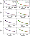 |
Fig. B.3. Errors in the angular correlation function, derived as the square root of diagonal elements of Covθiθj, in real (blue squares), redshift (with σz = 0, black circles) and photo-z space, with σz = 0.02, (red triangles) and σz = 0.05 (green triangles), from the numerical covariance matrix measured from 1000 mocks. The lines show the results obtained with the linear power spectrum in the Limber approximation (solid black line), with the exact integration given by Eq. (43), which also includes the modelling of the RSDs (dashed red line) and with the damped linear power spectrum in the Limber approximation (solid red and green lines). |
In Fig. B.3 we can see the errors in the angular correlation function, derived as the square root of the diagonal elements of Covθiθj, in real, in redshift and in photo-z space. As for Covℓℓ′, we notice that there is a good agreement between the numerical estimate and the theoretical model, with the former overestimating the latter by a maximum of 10%, in the interval 0.8 < z < 1.0. On the other hand, due to the range of angular scales involved, we see no differences between the Limber approximation and the Cℓ model including the RSDs. This is valid also for the measurements, since the ratio between the real-space and redshift-space errors is always greater than 0.95, meaning that there is no substantial difference between the two covariance matrices. In addition, we find that the theoretical red and green lines of Fig. B.3, for σz, 0 = 0.02 and σz, 0 = 0.05 respectively, get progressively closer as the redshift increases. This is due to the fact that, at z > 0.6, according to Eqs. (B.1) and hence (B.5), the errors becomes progressively more dominated by the shot noise and variations due to the Cℓ term, given by photo-z damping and RSDs, are no longer appreciable.
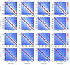 |
Fig. B.4. Comparison between measurements and model in the full set of the w(θ) correlation matrices. The rows correspond to the different redshift bins, while different columns refer to real, redshift, with σz, 0 = 0, and photo−z space, with σz, 0 = 0.02 and σz, 0 = 0.05, from left to right. The upper triangles show the numerical estimate made on 1000 mocks. The lower triangles show the normalised covariance model. |
In Fig. B.4 we can see the full set of correlation matrices. The rows correspond to the different redshift bins and indicate that the correlation decreases with z, while the columns refer to the analysis in real, redshift or photo−z space, with angular bins being less correlated in the presence of photo-z errors. The upper triangles show the numerical estimate made on 1000 PLCs. The lower triangles show the bin-averaged model presented in Eq. (B.10), where Cℓs are computed with the Limber approximation.
Appendix C: Investigating further observational systematics
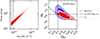 |
Fig. C.1. Mass proxy in cosmological analysis. Left panel: Mass-observable distribution of galaxy clusters in our mock catalogue. The grey shaded region represents the mass selection of our sample, excluding clusters with Mvir < 1014 M⊙ h−1. Right panel: Marginalised posterior distributions in the Ωm − σ8 plane, with 68% and 95% confidence intervals, using a binwidth of Δz = 0.4, in redshift space. The red contour shows the result for the two-point correlation function monopole, while the blue contour accounts also for the effect of the mass-observable scaling relation. The dashed lines indicate the Ωm and σ8 values of the PINOCCHIO simulation, while the dot-dashed line shows the predicted S8 degeneracy curve. |
Using observations at different wavelengths, it is possible to calibrate parametric scaling relations between the mass of galaxy clusters and a generic observable, Oobs, which can be used as mass proxy. The so-called mass-observable scaling relation represents a key link between the theoretical mass function and bias – with their cosmological dependence – and the distribution of clusters in the space of survey observables. However, this introduces a degeneracy with ΛCDM parameters, which might significantly degrade the constraining power of cluster clustering and other cluster cosmological probes.
Therefore, accurate constraints require us to properly take into account the dependence of the mass on these additional parameters. To quantify possible systematic uncertainties due to a non-accurate mass estimation, we model the scaling relation as
 (C.1)
(C.1)
where we fix  , Mpiv = 1014 M⊙ h−1 and zpiv = 0.60. Here, A, B and C represent the normalisation, the slope and the redshift evolution of the scaling relation, respectively. In practice, starting from the PINOCCHIO catalogue, we extract a value for Oobs according to a log-normal distribution, with a mean derived from Eq. (C.1) and a standard deviation equal to the intrinsic scatter, σintr:
![Mathematical equation: $$ \begin{aligned} P(\log O^\mathrm{obs}| M_{\rm vir}, z) = \frac{1}{\sqrt{2\pi } \sigma _{\rm intr}} \mathrm{exp}\left[ -\frac{ x^2 (O^\mathrm{obs}, M_{\rm vir},z)}{2\sigma _{\rm intr}^2} \right]. \end{aligned} $$](/articles/aa/full_html/2025/01/aa51566-24/aa51566-24-eq107.gif) (C.2)
(C.2)
Here ![Mathematical equation: $ x = \log (O^{\mathrm{obs}}/O^{\mathrm{obs}}_{\mathrm{piv}}) - [A + B \log (M_{\mathrm{vir}}/M_{\mathrm{piv}})+ C \log ((1+z)/(1+z_{\mathrm{piv}}))] $](/articles/aa/full_html/2025/01/aa51566-24/aa51566-24-eq108.gif) . We choose realistic parameters of the scaling relation, based on the state-of-the-art cosmological surveys (see e.g. Ghirardini et al. 2024), which are summarised in Table C.1, together with their respective uniform priors for the Bayesian inference.
. We choose realistic parameters of the scaling relation, based on the state-of-the-art cosmological surveys (see e.g. Ghirardini et al. 2024), which are summarised in Table C.1, together with their respective uniform priors for the Bayesian inference.
Parameters, descriptions, and priors used for the mass-observable scaling relation in Eq. (C.1).
The effective bias of the cluster sample is then estimated as
 (C.3)
(C.3)
using the bias model presented in Tinker et al. (2010) and the halo mass function model of Despali et al. (2016). Notably, the effective bias computed with Eq. (C.3) differs from the one derived with Eq. (10) by at most 2%, depending on the redshift bin.
We then repeat the MCMC analysis of Sect. 6, focusing for the sake of simplicity only on ξ0(s), in the case of Δz = 0.4 and in redshift space. The aim is to show the impact of the uncertainties in the mass determination and to compare them with other observational systematics, such as the photo-z errors. The results are shown in Fig. C.1. We found that Ωm and σ8 change from  and
and  , to
, to  and
and  , respectively. In particular, the relative error on σ8 increases from 9% to 12%, determining a general broadening in the posterior distribution of S8, which goes from
  to
to  , a value consistent, within 1σ, with the cosmology of the PINOCCHIO simulation. While the uncertainty in the scaling relation slightly dilutes the effect of non-linearities in cluster clustering, it leads to a significant degradation of the constraining power, comparable to that expected from the introduction of photo-z errors. This is due to the fact that the parameters of Eq. (C.1), and in particular the normalisation A, degenerate with the bias, thus allowing for a wider range of σ8 values to be explored. We conclude that an accurate prior on the scaling relation parameters is fundamental to avoid biases in cosmological constraints. Our result is in agreement with several previous works (see e.g. Costanzi et al. 2013; Sartoris et al. 2016), highlighting the fact that a precise and accurate knowledge of the scaling relation, achievable through robust mass calibration in current and forthcoming cosmological surveys, is necessary to maximise the information obtained from cluster number counts and cluster clustering.
We now briefly discuss some additional sources of uncertainty arising from observations. Galaxy clusters detected in real surveys are selected according to Oobs, so they are collected in catalogues that differ from mass-selected samples. This fact affects both the cluster abundance and the clustering properties. In particular, the clustering amplitude depends not only on the mass of the dark matter haloes, but also on secondary properties connected to their assembly history, such as the halo concentration, which in turn is related to their formation redshift. This phenomenon, which we refer to as the halo assembly bias (e.g. Gao et al. 2005), plays an important role in our understanding of structure formation. It has been shown in several numerical simulations, but it still remains elusive in observations at galaxy cluster scales, being degenerate with other systematic uncertainties (Zu et al. 2017). In particular, optically identified clusters tend to be enveloped in filaments along the line of sight and collect interlopers that artificially increase both the cluster richness and the final lensing mass, producing an anisotropic enhancement of the clustering signal (McClintock et al. 2019; Park et al. 2023). Moreover, this selection favours haloes with their major axis oriented along the line of sight. Projection and orientation effects modify the observed galaxy and matter overdensities of galaxy clusters, with respect to randomly selected haloes. According to To et al. (2021), these systematic uncertainties can be modelled on large scales as a mass-dependent multiplicative bias factor, which for the mass interval considered in our paper is between 15% and 20%. On the other hand, Park et al. (2023) present the scale dependent anisotropic boost as a multiplicative factor of the effective bias, which impacts the large scale regimes of cluster lensing and cluster clustering signal. In the radial range of the present analysis, its value assumes a maximum of 10%. The boost factor is measured to be at about the same level in a wide range of richness bins, also in Sunayama (2023), using a model which has been validated on mock cluster catalogues built from cosmological N-body simulations and applied to the Sloan Digital Sky Survey (SDSS) red-sequence Matchedfilter Probabilistic Percolation (redMaPPer, Rykoff et al. 2014) clusters.
Although a detailed study of these systematic uncertainties is beyond the scope of this paper, we emphasise that they should be properly modelled in real data analyses to mimimise biases in the estimation of cosmological parameters.
All Tables
Parameters, descriptions, and priors used for the mass-observable scaling relation in Eq. (C.1).
All Figures
|
Fig. 1. First three even multipoles of the 3D two-point correlation function measured from one PINOCCHIO PLC. The errors are computed as the square root of the diagonal elements of the covariance matrix. We show results for monopoles (white circles), quadrupoles (orange squares), and hexadecapoles (blue triangles). The different columns refer to redshift space with σz = 0, and to photo-z space with σz = 0.02(1 + z) and σz = 0.05(1 + z). The solid lines show the theoretical two-point correlation function multipoles, computed from the power spectrum estimated with CAMB, assuming a linear model with ΣNL = 0 (i.e. without non-linear damping effects at the BAO scale). They include systematic effects, such as RSDs and photo-z damping. The colour of the lines corresponds to the multipoles indicated by the symbols. |
| In the text | |
|
Fig. 2. Numerical correlation matrices of the 3D two-point correlation function first three even multipoles, derived from 1000 PLCs. The corresponding colour-bar is shown on the right. In the top panels the red diagonal separates the results for real space (upper triangles) and redshift space, with σz = 0 (lower triangles). In the bottom panels the red diagonal separates the results in photo-z space, where RSDs are included, for photo-z errors given by σz = 0.02(1 + z) (upper triangles) and σz = 0.05(1 + z) (lower triangles). In each panel the horizontal and vertical white solid lines separate the correlation sub-matrices of the monopole ξ0(r), the quadrupole ξ2(r), and the hexadecapole ξ4(r), and their corresponding cross-correlations. |
| In the text | |
|
Fig. 3. Angular two-point correlation function, measured from one PINOCCHIO PLC. The errors are computed as the square root of the diagonal elements of the covariance matrix. We show results for redshift space with σz = 0 (blue circles), and for photo-z space with RSDs, for photo-z errors equal to σz = 0.02(1 + z) (red squares) and σz = 0.05(1 + z) (green triangles). The solid lines show the theoretical two-point correlation function, computed from the power spectrum estimated with CAMB, assuming a linear model with ΣNL = 0 (i.e. without non-linear damping effects at the BAO scale). They include RSDs, and their colours correspond to the photo-z damping indicated by the symbols. |
| In the text | |
|
Fig. 4. Numerical correlation matrices of the angular two-point correlation function derived from 1000 PLCs (see colour-bar on the right). Left: results for real space (upper triangle) and redshift space, with σz = 0 (lower triangle). Right: results in photo-z space, where RSDs are included, for photo-z errors given by σz = 0.02(1 + z) (upper triangle) and σz = 0.05(1 + z) (lower triangle). In each panel the horizontal and vertical white solid lines separate the cross-correlation sub-matrices measured between different redshift bins. |
| In the text | |
|
Fig. 5. Redshift distribution of dark matter haloes, dN/dz, from a single realisation of PINOCCHIO PLC, with an angular radius of approximately 60 deg, in the redshift range 0.2 < z < 1.0. The coloured hatched histogram represented with a solid line shows the real-space redshift distribution, while the dashed histogram shows the photometric distribution, after the introduction of a Gaussian perturbation with σz = 0.05(1 + z). The light shaded regions give the limits of the photometric redshift bins of our tomographic analysis, with Δz = 0.2. The solid line gives the true dN/dz in the window function W, derived by integrating the halo mass function of Despali et al. (2016), assuming the cosmological parameters of the simulation. The dashed lines are derived through Eq. (38) and show the expected halo distribution in the ith redshift bin, selected by W. |
| In the text | |
|
Fig. 6. Angular power spectrum, measured from one PINOCCHIO PLC. The errors are computed as the square root of the diagonal elements of the covariance matrix. We show results for redshift space with σz = 0 (blue circles), and photo-z space with RSDs for photo-z errors equal to σz = 0.02(1 + z) (red squares) and σz = 0.05(1 + z) (green triangles). The solid lines show the theoretical angular power spectrum, computed from the power spectrum estimated with CAMB, assuming a linear model with ΣNL = 0 (i.e. without non-linear damping effects at the BAO scale). They include RSDs, and their colours correspond to the photo-z damping indicated by the symbols. |
| In the text | |
|
Fig. 7. Numerical correlation matrices of the angular power spectrum, derived from 1000 PLCs (see colour bar on the right). Left: results for real space (upper triangle) and redshift space, with σz = 0 (lower triangle). Right: results in photo-z space where RSDs are included, for photo-z errors given by σz = 0.02(1 + z) (upper triangle) and σz = 0.05(1 + z) (lower triangle). In each panel the horizontal and vertical white solid lines separate the cross-correlation sub-matrices measured between different redshift bins. |
| In the text | |
|
Fig. 8. Shot noise estimation over 100 realisations, using one realisation of the PINOCCHIO PLCs, in four redshift bins in the range 0.2 < z < 1.0 (panels from left to right). The red circles represent the angular power spectrum of the half-sum (HS) maps, which include the contribution of both signal and noise. The purple squares instead show the angular power spectrum of the half-difference (HD) maps, which provide a direct estimate of the shot noise, with their average (purple dashed line) and standard deviation (purple shaded band) in agreement with the theoretical Poissonian value (cyan solid line). |
| In the text | |
|
Fig. 9. Marginalised posterior distributions in the Ωm − σ8 plane, with 68% and 95% confidence intervals, for redshift and photo-z space, using a binwidth of Δz = 0.2 and Δz = 0.4, in the upper and lower panels, respectively. The contours are for w(θ) and Cℓ. The dashed lines indicate the Ωm and σ8 values of the PINOCCHIO simulation, while the dot-dashed line shows the predicted S8 degeneracy curve. |
| In the text | |
|
Fig. 10. Marginalised posterior distributions in the Ωm − σ8 plane, with 68% and 95% confidence intervals, for redshift and photo-z space, using a binwidth of Δz = 0.2 and Δz = 0.4, in the upper and lower panels, respectively. The contours are for the different multipoles of ξ(s). The dashed lines indicate the Ωm and σ8 values of the PINOCCHIO simulation, while the dot-dashed line shows the predicted S8 degeneracy curve. |
| In the text | |
|
Fig. 11. Summary plot for the parameter S8, in redshift and photo-z space with σz = 0.02(1 + z) and σz = 0.05(1 + z), panels from left to right, for w(θ) and ξ0(s). The solid lines refer to Δz = 0.2, the dashed lines to Δz = 0.4. The dot-dashed line indicates the S8 value of the PINOCCHIO simulation. |
| In the text | |
|
Fig. A.1. Mixing matrices for different sky coverages. Left panels: Colour plots of the mixing matrix, Rℓℓ′, computed up to ℓ = 500 with the public code NAMASTER (Alonso et al. 2019). Right panels: Plots of Rℓℓ*/Rℓ*ℓ*, centred in three different multipoles, at ℓ = 100 (blue), 150 (orange) and 200 (green). They quantify the mode-mode coupling related to the partial sky coverage, reflecting the blurring of the mixing matrix along the diagonal. The grey shaded regions indicate the multipole range of Δℓ in which we bin our measurements. The top panels are computed from the 10313 deg2 region covered by the full PINOCCHIO footprint mask, while at the bottom we focus on the 1004 deg2 subregion. |
| In the text | |
|
Fig. B.1. Errors in the angular power spectrum, derived as the square root of diagonal elements of Covℓℓ′, in real (blue squares), redshift (with σz = 0, black circles) and in photo-z space, with σz = 0.02, (red triangles) and σz = 0.05 (green triangles), from the numerical covariance matrix measured from 1000 mocks. The lines show the results obtained with the linear power spectrum in the Limber approximation (solid black line), with the exact integration given by Eq. (43), which also includes the modelling of the RSDs (dashed red line) and with the damped linear power spectrum in the Limber approximation (solid red and green lines). |
| In the text | |
|
Fig. B.2. Comparison between diagonal and non-diagonal errors on the real-space angular power spectrum, Cℓ, in different redshift bins. Grey squares and magenta pentagons are measured from the set of mocks, with the full PLCs sky coverage and with its 1000 deg2 subregions, respectively. The black lines are computed through the Limber approximation, with the diagonal |
| In the text | |
|
Fig. B.3. Errors in the angular correlation function, derived as the square root of diagonal elements of Covθiθj, in real (blue squares), redshift (with σz = 0, black circles) and photo-z space, with σz = 0.02, (red triangles) and σz = 0.05 (green triangles), from the numerical covariance matrix measured from 1000 mocks. The lines show the results obtained with the linear power spectrum in the Limber approximation (solid black line), with the exact integration given by Eq. (43), which also includes the modelling of the RSDs (dashed red line) and with the damped linear power spectrum in the Limber approximation (solid red and green lines). |
| In the text | |
|
Fig. B.4. Comparison between measurements and model in the full set of the w(θ) correlation matrices. The rows correspond to the different redshift bins, while different columns refer to real, redshift, with σz, 0 = 0, and photo−z space, with σz, 0 = 0.02 and σz, 0 = 0.05, from left to right. The upper triangles show the numerical estimate made on 1000 mocks. The lower triangles show the normalised covariance model. |
| In the text | |
|
Fig. C.1. Mass proxy in cosmological analysis. Left panel: Mass-observable distribution of galaxy clusters in our mock catalogue. The grey shaded region represents the mass selection of our sample, excluding clusters with Mvir < 1014 M⊙ h−1. Right panel: Marginalised posterior distributions in the Ωm − σ8 plane, with 68% and 95% confidence intervals, using a binwidth of Δz = 0.4, in redshift space. The red contour shows the result for the two-point correlation function monopole, while the blue contour accounts also for the effect of the mass-observable scaling relation. The dashed lines indicate the Ωm and σ8 values of the PINOCCHIO simulation, while the dot-dashed line shows the predicted S8 degeneracy curve. |
| In the text | |
Current usage metrics show cumulative count of Article Views (full-text article views including HTML views, PDF and ePub downloads, according to the available data) and Abstracts Views on Vision4Press platform.
Data correspond to usage on the plateform after 2015. The current usage metrics is available 48-96 hours after online publication and is updated daily on week days.
Initial download of the metrics may take a while.