| Issue |
A&A
Volume 682, February 2024
|
|
|---|---|---|
| Article Number | A72 | |
| Number of page(s) | 14 | |
| Section | Cosmology (including clusters of galaxies) | |
| DOI | https://doi.org/10.1051/0004-6361/202348305 | |
| Published online | 02 February 2024 | |
AMICO galaxy clusters in KiDS-DR3: Cosmological constraints from the angular power spectrum and correlation function
1
Dipartimento di Fisica e Astronomia “A. Righi” – Alma Mater Studiorum Università di Bologna, Via Piero Gobetti 93/2, 40129 Bologna, Italy
e-mail: This email address is being protected from spambots. You need JavaScript enabled to view it.
2
INAF – Osservatorio di Astrofisica e Scienza dello Spazio di Bologna, Via Piero Gobetti 93/3, 40129 Bologna, Italy
3
INFN – Sezione di Bologna, Viale Berti Pichat 6/2, 40127 Bologna, Italy
4
Universitäts-Sternwarte München, Fakultät für Physik, Ludwig-Maximilians-Universität München, Scheinerstrasse 1, 81679 München, Germany
5
INAF – Osservatorio Astronomico di Trieste, Via G. B. Tiepolo 11, 34143 Trieste, Italy
6
Dipartimento di Fisica “E. Pancini”, Università di Napoli Federico II, C.U. di Monte SantAngelo, Via Cintia, 80126 Napoli, Italy
7
INAF – Osservatorio Astronomico di Capodimonte, Salita Moiariello 16, 80131 Napoli, Italy
8
INFN – Sezione di Napoli, Via Cintia, 80126 Napoli, Italy
9
Zentrum für Astronomie, Universität Heidelberg, Philosophenweg 12, 69120 Heidelberg, Germany
10
ITP, Universität Heidelberg, Philosophenweg 16, 69120 Heidelberg, Germany
11
INAF – Osservatorio Astronomico di Padova, Vicolo dell’Osservatorio 5, 35122 Padova, Italy
Received:
18
October
2023
Accepted:
21
November
2023
Abstract
We study the tomographic clustering properties of the photometric cluster catalogue derived from the third data release of the Kilo Degree Survey (KiDS), focusing on the angular correlation function and its spherical harmonic counterpart: the angular power spectrum. We measured the angular correlation function and power spectrum from a sample of 5162 clusters, with an intrinsic richness of λ* ≥ 15, in the photometric redshift range of z ∈ [0.1, 0.6]. We compared our measurements with theoretical models, within the framework of the Λ cold dark matter cosmology. We performed a Markov chain Monte Carlo (MCMC) analysis to constrain the cosmological parameters, Ωm and σ8, as well as the structure growth parameter, S8 ≡ σ8√Ωm/0.3. We adopted Gaussian priors on the parameters of the mass-richness relation, based on the posterior distributions derived from a previous joint analysis of cluster counts and weak-lensing mass measurements carried out on the basis of the same catalogue. From the angular correlation function, we obtained Ωm = 0.32−0.04+0.05, σ8 = 0.77−0.09+0.13, and S8 = 0.80−0.06+0.08, which are in agreement, within 1σ, with the 3D clustering result based on the same cluster sample and with existing complementary studies on other data sets. For the angular power spectrum, we checked the validity of the Poissonian shot noise approximation, also considering the mode-mode coupling induced by the mask. We derived statistically consistent results, in particular, Ωm = 0.24−0.04+0.05 and S8 = 0.93−0.12+0.11; while the constraint on σ8 alone is weaker with respect to the one provided by the angular correlation function, σ8 = 1.01−0.17+0.25. Our results show that the 2D clustering from photometric cluster surveys can provide competitive cosmological constraints with respect to the full 3D clustering statistics. We also demonstrate that they can be successfully applied to ongoing and forthcoming spectrometric and photometric surveys.
Key words: cosmological parameters / large-scale structure of Universe
© The Authors 2024
 Open Access article, published by EDP Sciences, under the terms of the Creative Commons Attribution License (https://creativecommons.org/licenses/by/4.0), which permits unrestricted use, distribution, and reproduction in any medium, provided the original work is properly cited.
This article is published in open access under the Subscribe to Open model. This email address is being protected from spambots. You need JavaScript enabled to view it. to support open access publication.
1. Introduction
The spatial properties of the large-scale structure (LSS) of the Universe have been recognized as key cosmological probes. According to the Λ cold dark matter (ΛCDM) model, galaxy clusters are the largest gravitationally bound systems that emerge from the cosmic web of LSS (e.g. Kaiser 1984). They trace peaks in the large-scale matter density field, produced by gravitational infall and the hierarchical merging of dark matter halos (Bardeen et al. 1986; Tormen 1998; Despali et al. 2016). Since their growth is related to the expansion rate of the Universe and to the underlying distribution of matter, cluster statistics represent a powerful tool for understanding the structure formation process, constraining the neutrino mass (e.g. Marulli et al. 2011; Villaescusa-Navarro et al. 2014; Roncarelli et al. 2015), and investigating the nature of dark matter and dark energy (e.g. Mantz et al. 2008; Vikhlinin et al. 2009; Marulli et al. 2012; Sartoris et al. 2016; Costanzi et al. 2019; Moresco et al. 2021; Lesci et al. 2022a,b) as well as that of gravity itself (e.g. Marulli et al. 2021).
Despite the fact that cluster catalogues usually contain a lower number of objects with respect to galaxy catalogues, cosmology with clusters presents a series of key advantages. Galaxy clusters are hosted by the most massive virialised halos, so they are highly biased tracers, that is, they are more clustered than galaxies (e.g. Mo & White 1996; Moscardini et al. 2001; Sheth et al. 2001; Hütsi 2010; Allen et al. 2011; Moresco et al. 2021). Furthermore, thanks to their lower peculiar velocities, galaxy clusters are relatively less affected by nonlinear dynamics at small scales; in particular, by the effect of incoherent motions within virialised structures that generates the so-called fingers-of-God effect (e.g. Jackson 1972; Veropalumbo et al. 2014; Sereno et al. 2015; Marulli et al. 2017). The impact of redshift-space distorsion (RSD) is thus reduced, allowing us to simplify theoretical assumptions in the modelling of their clustering signal.
Over the past few years, cluster catalogues have been constructed from observations at several wavelengths (Allen et al. 2011), for example, by exploiting the X-ray emission from the diffuse intracluster medium (ICM; Rosati et al. 2002; Böhringer et al. 2004; Pacaud et al. 2016) and the millimeter Sunyaev–Zel’dovich effect produced by the inverse Compton scattering between the hot ICM electrons and the cosmic microwave background (CMB) photons (Vanderlinde et al. 2010; Planck Collaboration VIII 2011), as well as the optical and near-infrared (IR) starlight emission from galaxies (Eisenhardt et al. 2008; Bellagamba et al. 2018). The importance of this multiwavelength approach relies on the possibility to relate different observables, accessible with spectro-photometric observations, to the total mass of clusters, mostly composed of dark matter. The existence of a so-called mass-observable scaling relation (Okabe et al. 2010; Allen et al. 2011; Giodini et al. 2013; Sereno & Ettori 2015; Bellagamba et al. 2019; Sereno et al. 2020; Giocoli et al. 2021) represents a useful link between the theoretical mass function and the distribution of clusters in the space of survey observables and gives us the opportunity to predict the effective bias of the cluster sample (e.g. Branchini et al. 2017; Lesci et al. 2022b).
In recent decades, the cosmic distribution of the LSS has been investigated in a progressively more accurate and precise way. Typically, measurements of clustering are based on some cosmological assumption for the redshift-distance relation and require an appropriate reconstruction of the position of cosmic structures, which can be provided by spectroscopic redshift surveys, such as the Sloan Digital Sky Survey (SDSS; see Tegmark et al. 2004) or, more recently, the Baryon Oscillation Spectroscopic Survey (BOSS; see Tojeiro et al. 2012) and the Dark Energy Spectroscopic Instrument Legacy Survey (DESI; see Hang et al. 2021). However, spectroscopic surveys are time-consuming thus, in a given amount of observational time, they have a series of limitations in terms of sky coverage and numbers of detected objects. On the other hand, ongoing and future photometric surveys, such as the Kilo Degree Survey (KiDS; see de Jong et al. 2017; Kuijken et al. 2019), Dark Energy Survey (DES; see Dark Energy Survey Collaboration 2016), Hyper Suprime-Cam (HSC) Subaru Strategic Program (HSC-SSP; see Aihara et al. 2018), Vera C. Rubin Observatory Legacy Survey of Space and Time (LSST; see LSST Dark Energy Science Collaboration 2012) and Euclid mission (Laureijs et al. 2011; Scaramella et al. 2014; Amendola et al. 2018; Euclid Collaboration 2022) will allow us to cover a wider area, imaging also faint sources at high z.
One of the most powerful tools of modern cosmology is the analysis of the two-point correlation function. The simplest and historically first point-process statistics to be applied are: the two-point angular correlation function in the configuration space and its harmonic-space counterpart, namely, the angular power spectrum (Hauser & Peebles 1973; Peebles 1973). In principle, these two statistics bring on the same cosmological information, although in practice they have different sensitivities to different scales, due to the finite sizes of real catalogues and, thus, the limited range of scales that can be probed. One of their fundamental advantages with respect to the full 3D study is that we can measure the clustering signal from the angular position alone, without any cosmological assumption in converting redshifts to distances (Asorey et al. 2012; Salazar-Albornoz et al. 2014).
The aim of this work is to perform a cosmological analysis based on the catalogue of galaxy clusters identified by the Adaptive Matched Identifier of Clustered Objects (AMICO; see Bellagamba et al. 2018) algorithm from the third data release of the Kilo Degree Survey (KIDS-DR3), presented in Maturi et al. (2019). Here, the availability of photometric redshift measurements allows us to divide the catalogue into shells and to perform a “tomographic” study, which can provide independent constraints relative to the 3D reconstruction.
The current analysis has been performed with the COSMOBOLOGNALIB (Marulli et al. 2016)1, a set of free software C++ and Python libraries that we used to manage cluster catalogues, to measure their statistical quantities and to perform the Bayesian inferences. This work is part of a series of papers aimed at exploiting distant clusters in KiDS for both cosmological (Bellagamba et al. 2019; Giocoli et al. 2021; Ingoglia et al. 2022; Lesci et al. 2022a,b; Busillo et al. 2023) and astrophysical studies (Radovich et al. 2020; Puddu et al. 2021).
The paper is organised as follows. In Sect. 2, we present the AMICO KiDS cluster catalogue. In Sects. 3 and 4, we describe the methods used to measure and model the cluster angular correlation function and power spectrum, respectively. In Sect. 5, we discuss the results of the cosmological analysis. Finally, in Sect. 6 we give our conclusions.
2. Data: AMICO KiDS-DR3 catalogue
KiDS is a European Southern Observatory (ESO) public optical imaging survey, obtained with the OmegaCAM wide-field imager (Kuijken 2011) mounted on the 2.6 m Very Large Telescope (VLT) Survey Telescope (VST), at the Paranal Observatory. This work is focused on its third release, KiDS-DR3 (de Jong et al. 2017). The DR3 covers a total area of 438 deg2 over two fields, one equatorial (KiDS-N) and the other near the South Galactic Pole (KiDS-S), with aperture photometry in the u, g, r, and i bands down to the limiting magnitudes of 24.3, 25.1, 24.9, and 23.8, respectively. A final effective area of 377 deg2 (Maturi et al. 2019), displayed by the pixelated KiDS-DR3 footprint binary mask presented in Fig. 1 (Hildebrandt et al. 2017), which can be found on the KiDS website2, was obtained after rejecting all regions affected by satellite tracks, within halos produced by bright stars and within secondary or tertiary halo masks used for the weak lensing analysis (de Jong et al. 2015; Kuijken et al. 2015).
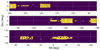 |
Fig. 1. KiDS-DR3 footprint binary mask (Hildebrandt et al. 2017), pixelated with HEALPIX (Górski et al. 2005), with a resolution given by Nside = 512. The top and the middle panels cover the extension of KiDS-N, while the bottom panel refers to KiDS-S. Clusters are distributed within the unmasked area (yellow). Small holes and irregularities reflect the presence of severe incompleteness and substantial photometric degradation, due to satellite tracks, stars etc. |
As discussed in Maturi et al. (2019), clusters were detected thanks to the application of the AMICO algorithm (Bellagamba et al. 2018), which identifies galaxy overdensities by exploiting a linear matched optimal filter. The cluster detection process relies only on the angular coordinates, magnitudes, and photometric redshifts of galaxies, avoiding a colour-based selection related to the red-sequence of clusters.
The complete sample contains 7988 objects, with a signal-to-noise ratio (S/N) > 3.5, in the redshift range z ∈ [0.10, 0.80]. We limit the current study to z ∈ [0.10, 0.60] because our model is based on the mass-richness scaling relation estimated from the stacked weak-lensing analysis presented in Bellagamba et al. (2019) and Lesci et al. (2022a), which has been calibrated in this photo-z range. The cluster detection algorithm returns an unbiased redshift estimate with respect to the input photometric catalogue, but it is sensitive to the photo-z bias of the underlying galaxy population, discussed in de Jong et al. (2017) for the KiDS survey. Thus, as suggested by Maturi et al. (2019), we correct the estimated cluster redshifts with the relation z = zest − 0.02(1 + zest).
The mass proxy for the scaling relation used in this paper is the intrinsic richness provided directly by AMICO, defined as the sum of the membership probabilities:
 (1)
(1)
where Pi(j) is the probability assigned by AMICO to the ith galaxy of being a member of a given detection, j; ri(j) is the distance of the ith galaxy from the centre of the jth cluster; R200(zj) is the sphere radius in which the mean density is 200 times the critical density at redshift zj; and m* is a function of redshift representing the typical magnitude used in the Schechter function of the cluster model employed by the AMICO algorithm (Maturi et al. 2019). Thus, for a given detection the intrinsic richness represents the expected number of visible galaxies, under the condition expressed in Eq. (1). According to this definition, it is a nearly redshift-independent quantity because the threshold m* + 1.5 is well below the magnitude limit of the galactic sample, in the considered redshift interval. For our analysis, we selected clusters with λ* ≥ 15, which ensures a purity higher than 97% and a completeness higher than 50% over the whole sample (Maturi et al. 2019). Finally, to perform a tomographic analysis, we split our catalogue in three different redshift bins. Thinner shells preserve clustering information along the line of sight and are closer to a full 3D study (Asorey et al. 2012; Salazar-Albornoz et al. 2014; Balaguera-Antolínez et al. 2018), but they reduce the projected number density of clusters and, thus, the accuracy and the precision of the measurements (Salazar-Albornoz et al. 2014). The redshift bin width was chosen to be five times larger than the maximum photometric error, while we increased the amplitude of the first redshift shell to improve the statistics. The final sample contains 5162 clusters, 1019 in z ∈ (0.10, 0.30], 2072 in z ∈ (0.30, 0.45], and 2071 in z ∈ (0.45, 0.60].
3. Angular correlation function of AMICO KiDS-DR3 catalogue
In this section, we describe the methods used to measure and model the angular correlation function.
3.1. Angular correlation function estimator
The joint probability of finding two clusters in the solid angle elements δΩ1 and δΩ2, at a distance θ is given by:
![Mathematical equation: $$ \begin{aligned} \delta P(\theta ) = n_{\Omega }^2[1+{ w}(\theta )]\delta \Omega _1 \delta \Omega _2, \end{aligned} $$](/articles/aa/full_html/2024/02/aa48305-23/aa48305-23-eq9.gif) (2)
(2)
where nΩ is the mean number of clusters per unit solid angle. Thus, the angular correlation function w(θ) represents the excess probability of finding a pair of objects separated by the angular distance θ, relative to that expected from a random distribution. We measured the observed angular correlation function using the Landy & Szalay (1993, LS) estimator:
 (3)
(3)
where DD(θ), RR(θ), and DR(θ) are the number of data-data, random-random, and data-random pairs in the angular bin θ ± Δθ/2, respectively. The measurement is performed in eight logarithmically-spaced bins, between 10−20 and 200 arcmin, with a conservative angular separation which takes into account the maximum virial cluster size in every redshift bin (for the lower limit) and the angular scale of the survey (for the upper limit). The results are shown for each redshift bin in Fig. 2, where they are also compared to the model presented in Sect. 3.2 and to the result of the cosmological analysis of Sect. 5.2, where we also provide a discussion about the excess of clustering detected in the last redshift bin.
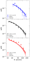 |
Fig. 2. Angular correlation function measured in three redshift bins: z ∈ (0.10, 0.30] (blue circles), z ∈ (0.30, 0.45] (black squares), z ∈ (0.45, 0.60] (red triangles). Error bars are estimated as the diagonal terms of the jackknife covariance matrix. The dashed lines represent the model computed with cosmological parameters by Planck Collaboration VI (2020, Table 2, TT, TE, and EE+lowE). The solid lines show the median of the model distribution computed from the combined posterior of our cosmological analysis, while the shaded regions highlight the 68% confidence levels. |
We constructed the random catalogue by randomly extracting the angular (RA, Dec) cluster coordinates within the survey observational tiles, using the same masks adopted in Maturi et al. (2019). To limit shot noise effects, our random catalogue is 30 times larger than the original one. The covariance matrix is estimated through the jackknife method (Norberg et al. 2009). Specifically, for each redshift slice, we projected our catalogue onto the celestial sphere, using the equal-area HEALPIX pixelisation scheme (Górski et al. 2005, see Sect. 4.1), with a low-resolution Nside = 128, that is, corresponding to a pixel side of 27 arcmin. Clusters belonging to the same pixel are considered part of a unique region. Therefore, the exact number of regions depends on the quantity of clusters available in each redshift bin and is of the order of 1000. This allows us to estimate the covariance matrix with different NJK measurements of the angular correlation function, obtained after removing one region at a time.
3.2. Angular correlation function model
On linear scales, the cluster density field, δcl(x), is related to the dark matter density field, δDM(x), through a scale-independent bias, bcl(z):
 (4)
(4)
which implies that in the Fourier space,  , where ncl(x) is the cluster density,
  is its mean value and PDM(k) is the linear dark matter power spectrum. We employed the fitting formulae provided by Eisenstein & Hu (1998), which in the angular range of our w(θ) and Cℓ analyses produce consistent results to those provided by CAMB (Lewis et al. 2000) and CLASS (Lesgourgues 2011; Blas et al. 2011). Given the normalised selection function ϕi(z) in the ith photometric redshift bin (see Sect. 3.3), we can project the density field onto the celestial sphere, in a given direction
  on the sky:
 (5)
(5)
The angular correlation function at a given separation θ is the projection of the 3D spatial correlation function, ξ(s):
 (6)
(6)
where  and r(z) is the comoving distance at redshift z. In this work, we assume the plane-parallel approximation and we parameterise the linear power spectrum in redshift space as:
 (7)
(7)
where  is the linear growth rate, μ is the cosine of the angle between k and the line of sight and beff is the effective bias, namely, the halo bias weighted with the halo mass function (see Sect. 3.4). The Fourier transform of the power spectrum gives us the 3D correlation function, which can be expressed in terms of multipoles ξl(s) and Legendre polynomials Pl(μ) (Hamilton 1992):
 (8)
(8)
We keep only the monopole because it includes most of the information (Salazar-Albornoz et al. 2014; García-Farieta et al. 2020). It can be written as a function of the real-space correlation function, ξDM(r):
![Mathematical equation: $$ \begin{aligned} \xi _0(s) = \left[b^2_{\mathrm{eff} }+\frac{2}{3}b_{\mathrm{eff} }f+\frac{1}{5}f^2 \right]\xi _{\mathrm{DM} }(r). \end{aligned} $$](/articles/aa/full_html/2024/02/aa48305-23/aa48305-23-eq21.gif) (9)
(9)
3.3. Redshift selection function model
Photometric redshifts have larger uncertainties than spectroscopic ones. Because of photo-z errors, cluster photometric redshift distributions can be different from the true redshift distributions, thus we need to account for the conditional probability of having a cluster at the true redshift, z, given the observed redshift, zphot.
In Eqs. (5) and (6), we consider the radial selection function as the normalised cluster distribution in a given redshift bin Δzi. In other words, it represents the probability of including a cluster in the corresponding photometric shell, depending on the selection characteristics of our study, namely on the binning strategy (Asorey et al. 2012). Our photometric volume-limited survey is selected by the top-hat window function:
 (10)
(10)
where zmin and zmax represent the lower and the upper limits of our photometric redshift interval, respectively. Including objects into redshift shells of a given redshift width Δzi allows us to “integrate out” the effect of photo-z errors (Bykov et al. 2023). The conditional probability of detecting a cluster in a sample selected with this window function, namely, our normalised redshift distribution, is obtained with the following convolution (Budavári et al. 2003; Crocce et al. 2011; Hütsi et al. 2014):
 (11)
(11)
where ϕ(z) is the true underlying full redshift distribution:
 (12)
(12)
and P(zphot|z) is a Gaussian distribution, as derived by Lesci et al. (2022a,b) from the mock catalogues described in Maturi et al. (2019), whose mean is z, while the standard deviation is equal to:
 (13)
(13)
with σz, 0 = 0.02. An estimate of the true redshift distribution can be then obtained as follows:
 (14)
(14)
where Ωsky is the survey area in rad2. Here, the cosmological dependence is provided by  , the derivative of the comoving volume, by
  , the halo mass function modelled with the functional form by Tinker et al. (2008), and by P(λ*|M, z), where λ* is the intrinsic richness. The latter integral convolves the theoretical mass function, taking into account the shape of the mass-observable scaling relation of the cluster sample (Lesci et al. 2022a):
 (15)
(15)
where P(λ*|z) is a cosmology-independent power-law with an exponential cut-off calibrated from mock catalogues (Lesci et al. 2022a), P(M|z) is a normalisation factor computed as the integral of the numerator, P(M|λ*, z) is modelled as a log-normal distribution, in which the mean is given by the mass-observable scaling relation and the root mean square is a free parameter of the model:
 (16)
(16)
Here,
 (17)
(17)
where E(z)≡H(z)/H0. We set λpiv = 30 and zpiv = 0.35, which represent the central values of intrinsic richness and redshift in the ranges covered by the whole sample, as found by Bellagamba et al. (2019). The intrinsic scatter is modelled with two free parameters, σintr, 0 and σintr, λ*, as follows:
 (18)
(18)
Finally, we need to compute the cluster redshift distribution in a given redshift bin, accounting also for the probability of measuring  given the true intrinsic richness, λ*, and modelling the selection effects and the incompleteness of the sample. This requires a further convolution in the intrinsic richess bin
  , with a Gaussian
  . We considered an uncertainty of 17% on
  , as in Lesci et al. (2022a,b). In Fig. 3, we show the KiDS-DR3 photometric redshift distribution and the complete number counts model, expressed by:
 (19)
(19)
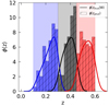 |
Fig. 3. Normalised redshift distributions. The histograms represent ϕ(zphot), from the photometric cluster catalogue, while ϕ(ztrue|W) is predicted from Eq. (11), using the theoretical halo mass function model by Tinker et al. (2008), with cosmological parameters provided by Planck Collaboration VI (2020, along with Table 2, TT, TE, and EE+lowE), then convolved with our photometric window function, W. The shaded areas indicate the limits of our photometric redshift bins. |
3.4. Effective bias of the cluster sample
Under the assumption that clusters trace the locations of the large-scale dark matter halos, we adopt a simple linear relation between dark matter and cluster power spectra:  . While, in general, the bias is expected to be a function of scale, at large linear scales it can be considered as a scale-independent quantity (e.g. Estrada et al. 2009; Manera & Gaztañaga 2011; Sawangwit et al. 2011). On the other hand, the evolution of both dark matter and cluster clustering leads to a bias which is a function of halo mass and redshift (Estrada et al. 2009).
Following the approach of Lesci et al. (2022b), we assume a constant bias, neglecting any redshift evolution within the broad photometric shell. The effective bias is derived theoretically, as the average over the number of clusters, Ni, in the photometric sample:
 (20)
(20)
where b(M, z) is the halo bias, according to the model presented in Tinker et al. (2010).
4. Angular power spectrum of AMICO KiDS-DR3 catalogue
In this section, we describe the methods used to measure and model the angular power spectrum.
4.1. Pixelated density map
For every different redshift bin, we generate a cluster density map by projecting the catalogue objects onto the celestial sphere, using the HEALPIX pixelisation (Górski et al. 2005), with a resolution of Nside = 512, which ensures a pixel size of approximately 7 arcmin, comparable with the minimum angular scale exploited in the w(θ) analysis. The density contrast, δcl, I, in each pixel I is given by:
 (21)
(21)
where ncl, I is the cluster number density in the Ith pixel and  is its mean, computed in the unmasked area of the survey. The pixelisation procedure smooths information on scales smaller than the pixel size, i.e. ℓ > 1500, which is, in our case, well above the maximum value of ℓ used in our analysis. Different observational effects, like stellar density, air-mass, sky flux, and reddening might introduce biases in the galaxy photometry, if not taken into account (Loureiro et al. 2019). This could lead to biases in the cluster detection, thus in the clustering statistics. In any case, regions affected by these effects are already excluded, since we estimate the cluster density in the unmasked field only, given by the KiDS-DR3 footprint binary mask. Furthermore, as Maturi et al. (2019) imposed the strict magnitude cut at r = 24 (note: the limit in the r band for KiDS-DR3 is 24.9; see Sect. 2), corresponding to the depth of the shallowest tile, the mean cluster count does not depend on the sky position (Lesci et al. 2022b). For these reasons and following, for example Branchini et al. (2017), clusters are counted as single objects, thus no weighting scheme has been applied to account for their selection effects. In Fig. 1, we show the KiDS-DR3 footprint mask, degraded from a resolution of Nside = 2048 to Nside = 512, keeping the 377 deg2 survey area, which yields to a final unmasked sky fraction of fsky ≈ 0.9%. The irregular geometry of KiDS-DR3 survey is reflected in the large number of small holes contained in the mask. Thus, we avoid any apodisation of the mask, which would lead to a significant modification in the shape and to a non-trivial loss of area (White et al. 2022).
4.2. Angular power spectrum estimator
The angular power spectrum of clusters in a given redshift bin, i, can be measured from the harmonic decomposition of the observed density field. The pixelated density contrast, being defined on a 2D sphere, can be expanded in a series of spherical harmonics:
 (22)
(22)
where Yℓm are the spherical harmonics, computed at the direction on the sky,  , aℓm, are the harmonic coefficients, defined by:
 (23)
(23)
the symbol * indicates the complex conjugation operator, while ΔΩI is the area of the Ith pixel. In this analysis, we used the angular power spectrum estimator introduced by Peebles (1973) and Hauser & Peebles (1973). For a partial sky survey, the masked density contrast is related to the full-sky field through a binary mask function,  ; thus, the measured pseudo-Cℓ in Fig. 4, named
  , is corrected for the sky fraction and defined as follows:
![Mathematical equation: $$ \begin{aligned} K^{ij}_\ell =\frac{1}{{ w}^2_\ell }\left[\frac{1}{f_{\mathrm{sky} }(2\ell +1)}\sum _{m=-\ell }^{m=\ell } |a^i_{\ell m}a^{*j}_{\ell m}|- \frac{\Delta \Omega }{N_{\mathrm{cl} }}\delta ^{ij}_K\right], \end{aligned} $$](/articles/aa/full_html/2024/02/aa48305-23/aa48305-23-eq47.gif) (24)
(24)
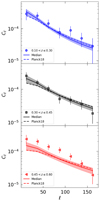 |
Fig. 4. Angular power spectrum measured in three redshift bins: z ∈ (0.10, 0.30] (blue circles), z ∈ (0.30, 0.45] (black squares), and z ∈ (0.45, 0.60] (red triangles). Error bars are estimated as the diagonal terms of the jackknife covariance matrix. The dashed lines represent the model computed with cosmological parameters by Planck Collaboration VI (2020, Table 2, TT, TE, and EE+lowE). The solid lines show the median of the model distribution computed from the combined posterior of our cosmological analysis, while the shaded regions highlight the 68% confidence levels. |
where wℓ is the HEALPIX pixel window function, which removes the effect of the pixelisation, depending on the parameter Nside.
The case i = j refers to the auto power spectrum, while i ≠ j to the cross power spectrum between different redshift bins. We removed the shot noise contribution from the measured power spectrum, which accounts for the unclustered part of the measure, given by a discrete distribution of point-like sources. In a first approximation, it depends only on the ratio  , where
  is the Kronecker delta, equal to zero in the cross-correlation case. Possible deviations from this term are further investigated in Sect. 4.3. Due to the limited size of our cluster catalogues, the shot noise becomes the dominant part of the total signal at angular scales: ℓ ≳ 100 − 150, i.e. θ ≲ 1.8 − 1.2 deg, depending on the redshift bin.
As the KiDS-DR3 catalogue does not cover the full-sky, spherical harmonics no longer provide a complete orthonormal basis to expand the angular overdensity field (Camacho et al. 2019). Thus, the measured power spectrum at multipole ℓ depends on an underlying range of multipoles ℓ′ (Blake et al. 2007). This mode-mode coupling determines a power transfer between different multipoles and it is summarised in Rℓℓ′, the so-called mixing matrix, which depends only on the geometry of the angular mask. The ensemble average of the measured power spectrum is related to the theoretical one through (Balaguera-Antolínez et al. 2018):
 (25)
(25)
The mixing matrix is equal to an identity matrix in full-sky surveys, where fsky = 1. Starting from the survey window function, Rℓℓ′ can be expressed in terms of the Wigner 3j symbols:
 (26)
(26)
where:
 (27)
(27)
and Iℓm represents the spherical harmonic coefficient of the mask, given by:
 (28)
(28)
We estimate the mixing matrix using the publicly available code NAMASTER (Alonso et al. 2019), which provides a general framework for the pseudo-Cℓ analysis. The convolution function Rℓ*ℓ′ is shown in Fig. 5. It is peaked at ℓ*, while it has a drop at different multipoles, depending on the survey area and geometry. In this sense, the mixing matrix gives us an indication about the size of Δℓ bands used to bin the measurements. Indeed, with Δℓ = 25 we can keep most of the clustering signal, reducing both the effect of the window function, the size of the covariance matrix and the correlation between different bands (Blake et al. 2007; Balaguera-Antolínez et al. 2018; Loureiro et al. 2019).
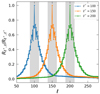 |
Fig. 5. Normalised elements of the mixing matrix Rℓℓ′, centred in three different multipoles ℓ* = 100, 150, 200. The functions decrease as we move away from ℓ*. Their value give us a quantitative amount of the correlation between different multipoles, induced by the mask. The gray shaded regions indicate the bin width Δℓ = 25 of our analysis. |
For each bin we compute the weighted average:
 (29)
(29)
After the convolution with the mixing matrix, the theoretical Cℓ is averaged with the same weights. As shown in Fig. 4, the redshift interval 0.45 < z ≤ 0.60 reveals the same excess of clustering detected in the w(θ) measurement (see Sect. 3.1). We offer a more in-depth discussion on this aspect in Sect. 5.2. We restricted our analysis to the range 10 < ℓ < 175. Although, in principle, a cautious limit for the maximum reachable scale is linked to the sky fraction through the relationship ℓmin = π/(2fsky) (Bernal et al. 2019), in practice, the effect of the partial sky coverage is already corrected by Eq. (25). This allows us to extend our analysis to larger scales which contain valuable cosmological information and to choose the lower limit according to the validity of the Limber approximation, while the upper is a conservative value that accounts for the impact of the shot noise (Balaguera-Antolínez et al. 2018), beyond which the clustering signal can be considered negligible.
The analytical error estimation adopted in Blake et al. (2007), Thomas et al. (2011), Balaguera-Antolínez et al. (2018), and Camacho et al. (2019) contains contributions from the cosmic variance and the shot noise, with a boost factor of  (Blake et al. 2007; Thomas et al. 2011). It is based on the assumption that the coefficients aℓm are Gaussian-distributed, while the effect of the angular window function is modelled by the parameter fsky (Blake et al. 2007; Balaguera-Antolínez et al. 2018), resulting in a diagonal covariance matrix. These approximations do not hold in our case, due to the irregular shape of the KiDS-DR3 survey, which introduces a non-negligible correlation between different multipoles, resulting in an error leak towards other ℓ modes and in a reduction of the diagonal errors (Crocce et al. 2011). Thus we estimated random errors directly from the dataset, using jackknife resampling. In practice, we divided our binary mask in NJK = 400 non-overlapping regions, removing one of them at a time. The cluster density field and the survey area used for the angular power spectrum measurements are then updated, for every realisation, by multiplying the original HEALPIX map by the new mask.
4.3. Shot noise correction
The quantity measured with Eq. (24) is the sum of two contributions: the signal and the shot noise. The latter represents the unclustered part of the power spectrum caused by the discreteness of the cluster distribution. The Poisson sampling of point-like sources contributes to the auto-correlation at null separation, in real space, which brings to a constant power spectrum in harmonic space (Paech et al. 2017), equal to  . However, when dealing with real data, this simple relation may not always hold. We verify the validity of the analytical relation for the shot noise in two steps. First, we check the power spectrum of 100 density maps derived from random cluster positions within the unmasked regions, considering the same number of cluster as in the real AMICO-KiDS catalogue. We find that the coupling with irregular mask merely increases the dispersion of the shot noise power spectrum around its theoretical prediction, with respect to full-sky surveys, without altering its mean value. Second, we expect deviations from the Poissonian shot noise due to halo exclusion and nonlinear effects (Giocoli et al. 2010; Baldauf et al. 2013). The exclusion simply consists in the fact that clusters cannot overlap, namely, the distance between clusters cannot be smaller than the sum of their radii, R (Baldauf et al. 2013; Paech et al. 2017). In other words, the cluster-cluster real-space correlation function ξcc(r) = − 1, for r < R, which means that the probability of finding another cluster is zero (Baldauf et al. 2013). The exclusion introduces a mass-dependent deviation from the Poissonian shot noise, since objects with different mass occupy different fractions of the sampling volume, while the nonlinear clustering effectively increases the noise term (Paech et al. 2017).
To test the robustness of the Poissonian shot noise hypothesis at the angular scales of our interest, we need a practical way to disentangle the signal and noise. Following Ando et al. (2018), Makiya et al. (2018) and Ibitoye et al. (2022), we first randomly divided the catalogue into two submaps, δ1, cl and δ2, cl, both of which contain roughly the same number of clusters. Then we build the half-sum,  , and the half-difference density fluctuation maps,
  . By construction, the former contains both signal and noise, while in the latter, the signal cancels out, leaving only the shot noise contribution. Since the division of the catalogue into subsets is a random process, the estimated HD map and its power spectrum
  slightly change for different realisations (Ando et al. 2018). Thus we averaged over 100 realisations, finding that the shot noise approximation holds in every redshift bin for all the multipoles considered in our analysis. In Fig. 6 we show the ensamble average of
  and
and  power spectra and the comparison with the Poissonian shot noise. Due to the very low number of clusters in our redshift bins, following Loureiro et al. (2019) we included an extra shot noise term, such that
  . The 𝒮i nuisance parameters are forward-modelled at the likelihood level, allowing them to vary within a Gaussian prior given by a mean equal to zero and the same standard deviation of
  , as shown in Table 1.
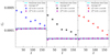 |
Fig. 6. Shot noise estimation over 100 realisations. Blue dots, black squares and red triangles represent the angular power spectrum of the half-sum (HS) maps, which contain the contribution of both signal and noise, in our three redshift bins (panels from left to right). The purple pentagons show instead the angular power spectrum of the half-difference (HD) maps, which provides a direct estimation of the shot noise, with their average (purple dashed line) and their standard deviation (purple shaded band) in agreement with the theoretical Poissonian value (cyan solid line). |
Parameters, prior and posterior mean, and percentiles of the cosmological analyses.
4.4. The angular power spectrum model
The angular power spectrum is modelled from the spatial power spectrum through a projection kernel, which takes into account the redshift evolution and radial selection effects. Its exact computation is given by (Padmanabhan et al. 2007; Thomas et al. 2011; Asorey et al. 2012; Camacho et al. 2019):
![Mathematical equation: $$ \begin{aligned} C_{\ell }^i = \frac{2}{\pi } \int \, \mathrm{d}k \, k^2 P_{\mathrm{DM} }(k) \left[\Psi _{\ell }^i(k) +\Psi ^{i,r}_\ell (k)\right]^2. \end{aligned} $$](/articles/aa/full_html/2024/02/aa48305-23/aa48305-23-eq67.gif) (30)
(30)
The kernel function  describes the mapping of k to ℓ in real space and is defined as:
 (31)
(31)
where ϕi(z) and b(z) are computed with Eqs. (11) and (20), respectively, jℓ(x) is the spherical Bessel function and D(z) is the linear growth factor, normalised such that D(0) = 1 (Camacho et al. 2019). The second term incorporates the linear Kaiser effect (Padmanabhan et al. 2007; Asorey et al. 2012), i.e. the enhancement in 3D power spectrum due to cluster peculiar velocities:
![Mathematical equation: $$ \begin{aligned} \begin{aligned} \Psi ^{i,r}(k)=&\int \mathrm{d}z \phi ^i(z) f(z) D(z) \left[\frac{2\ell ^2+2\ell -1}{(2\ell +3)(2\ell -1)} j_\ell (kr(z))\right.\\&-\frac{\ell (\ell -1)}{(2\ell -1)(2\ell +1 )}j_{\ell -2}(kr(z))\\&\left.- \frac{(\ell +1)(\ell +2)}{(2\ell +1)(2\ell +3)}j_{\ell +2}(kr(z)) \right]. \end{aligned} \end{aligned} $$](/articles/aa/full_html/2024/02/aa48305-23/aa48305-23-eq70.gif) (32)
(32)
Cluster peculiar velocities are smaller with respect to galaxy ones, thus, they only have a minor effect in our broad redshift selection function, and RSDs are erased by the radial projection (Padmanabhan et al. 2007). In particular, for ℓ ≫ 0, the term Ψi, r tends to zero, so that the total window function reduces to Eq. (31) (Padmanabhan et al. 2007; Thomas et al. 2011). However, since the evaluation of spherical Bessel functions is still quite computationally demanding, we make use of the Limber approximation (Limber 1953):
 (33)
(33)
where H(z) is the Hubble parameter and the photo-z effects are included through the radial selection function, ϕ(z) (Asorey et al. 2012), see Sect. 3.3. Here we underline that PDM(k, z) = PDM(k)D(z)2 is strictly valid only in linear theory (Blake et al. 2007).
Finally, there are two ways to consider the mode-mode coupling induced by the mask. We can solve the linear system in Eq. (25). This requires us to bin the pseudo-Cℓ into even more larger bandpowers, since it is computationally expensive and unstable to deconvolve the effect of the mixing matrix from our noisy data (Andrade-Oliveira et al. 2021). For this reason, we decide to include the angular selection directly at the level of the likelihood analysis, choosing the forward modelling (Balaguera-Antolínez et al. 2018; Loureiro et al. 2019; Xavier et al. 2019).
In Fig. 7 we show how redshift-space distortions and partial sky convolution can alter the shape of the angular power spectrum. In particular, the effect of the Limber approximation can be noted only for ℓ ≲ 10, namely, for multipoles that have already been excluded from our analysis. On the other hand, modifications due to the mixing matrix affect much smaller scales (ℓ ≲ 150); thus, we need to properly include them in our model.
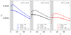 |
Fig. 7. Theoretical angular power spectrum for our three redshift bins. The Limber approximation is represented with a dotted line, while the exact computation is presented in Eqs. (31) and (32) with a dashed line. The convolution with the mixing matrix is shown, respectively, with a solid line (Limber approximation, i.e. the model used in our analysis), and with a dot-dashed line (exact computation). After the mode-mode coupling, the Limber approximation deviates only for ℓ ≲ 10, i.e. for the angular range already excluded from our analysis (gray shaded region). |
5. Cosmological analysis
5.1. Likelihood
The analyses of the angular correlation function and power spectrum are performed through Bayesian statistics. We estimate the set of cosmological parameters in Table 1, which enter the model, m, by adopting a Gaussian likelihood:
 (34)
(34)
in the kth redshift bin, where:
 (35)
(35)
where N is the number of angular bins, μ is the correlation statistic involved, namely, angular correlation function or power spectrum and the superscripts d and m refer to the quantities obtained from the data and computed with the model, respectively.  is the inverse of the covariance matrix in the kth redshift bin, estimated directly from the data for NJK jackknife resamplings (for example Norberg et al. 2009):
 (36)
(36)
with expectation values  . We neglected the correlations between different redshift slices, so that the total likelihood is simply given by the product of the individual likelihoods, ℒk.
5.2. Cosmological results
The Bayesian analysis was performed by adopting uniform priors on both Ωm and σ8, for which the cluster clustering is more sensitive, while we assumed Gaussian priors around the mean values from Planck Collaboration VI (2020, Table 2, TT, TE, and EE+lowE) for the baryon density, Ωb, the primordial spectral index, ns, and the normalised Hubble constant, h. The latter are not constrained by the clustering information contained in our measurements; indeed, when we repeated the analysis with flat priors in the same interval, we simply find that their posterior distributions cover the full range of the priors, without any significant impact on S8. We also used Gaussian priors for α, β, γ, σintr, 0 and σintr, λ*, the parameters of the mass-richness scaling relation, whose medians and standard deviations are taken from the posterior distribution of the cluster counts and weak lensing joint analysis, as derived by Lesci et al. (2022a). The full list of parameters is summarised in Table 1.
In Fig. 8, we show the results of the Markov chain Monte Carlo (MCMC) cosmological analysis, in the Ωm − σ8 plane. For the angular correlation function, we find  and
and  as the medians, namely, the 16th and the 84th percentiles of the marginalised 1D posterior distributions. The constraint on the structure growth parameter,
  , is presented in Fig. 9 as our main outcome, and compared with several previous studies available in the literature. In particular, we find a 1σ agreement with cosmological constraints from Wilkinson Microwave Anisotropy Probe (WMAP, Hinshaw et al. 2013, Table 3, WMAP-only, Year 9) and Planck (Planck Collaboration VI 2020, Table 2, TT, TE, and EE+lowE). An equivalent level of agreement is found also with the number counts analysis presented in Lesci et al. (2022a) using the same AMICO KiDS-DR3 cluster sample, in Costanzi et al. (2019), based on SDSS-DR8 cluster data, in Bocquet et al. (2019) with the 2500 deg2 South Pole Telescope – Sunyaev–Zel’dovich (SPT–SZ) survey data and with constraints from cosmic shear in DES Year 3 (Amon et al. 2022; Secco et al. 2022), HSC Year 3 (Dalal et al. 2023; Li et al. 2023) and KiDS-DR4 (Asgari et al. 2021). Instead, we note a 1σ tension with S8 from cluster abundances and weak lensing in DES Year 1 data (Abbott et al. 2020), probably related to richness-dependent effects, since it significantly reduces when their sample is limited to clusters with λ* ≥ 30.
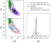 |
Fig. 8. Cosmological constraints in the Ωm − σ8 plane, with 68% and 95% confidence intervals, obtained considering angular power spectrum (green contours) and correlation function (purple contours). Our findings are compared to the cosmological constraints derived from Planck Collaboration VI (2020) (top left) and from the same KiDS-DR3 cluster catalogue (bottom left), in particular: the number counts and 3D correlation function analyses presented in Lesci et al. (2022a,b). Right: summary plot containing the 1D marginalised posteriors for the structure growth parameter, S8. |
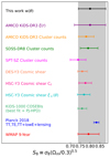 |
Fig. 9. Comparison of the constraints on S8, given by the posterior median, the 16th and the 84th percentiles. From top to bottom: Angular cluster clustering in the AMICO KiDS-DR3 catalogue obtained in this work (black dot); 3D cluster clustering from Lesci et al. (2022b, purple dot); cluster counts from Lesci et al. (2022a, orange dot), Costanzi et al.(2019, green dot) and Bocquet et al. (2019, magenta dot); cosmic shear from Amon et al. (2022); Secco et al. (2022, coral dot), Li et al. (2023, pink dot), Dalal et al.(2023, cyan dot) and Asgari et al. (2021, pale green dot); CMB results from Planck Collaboration VI (2020, blue dot) and Hinshaw et al. (2013, red dot). |
Concerning the “cluster clustering”, our main achievement shows the competitiveness of the 2D correlation function with respect to its 3D counterpart. Indeed, the current study provides more constraining power than the 3D correlation case discussed in Lesci et al. (2022b), where the measurement of ξ(r) is performed within two redshift bins: 0.1 ≤ z ≤ 0.3 and 0.35 ≤ z ≤ 0.6. This is partially due to the slightly larger sample considered, with 228 more clusters, and highlights the importance of the tomographic strategy adopted in photometric redshift surveys, for which several parameters, such as the bin width, the photometric redshift error, and the number density of detections, need to be balanced, as discussed in Sect. 2. Our tighter constraints are also confirmed by repeating the full MCMC analysis over 1000 bootstrap resampling, with replacement, which yields  ,
,  and
and  , in excellent agreement with our findings.
The angular power spectrum analysis includes an extra shot noise parameter for each redshift bin, with a Gaussian prior derived with the methodology described in Sect. 4.3. As shown in Fig. 8 the angular correlation function and the angular power spectrum produce statistically consistent results, although the latter exhibits a much lower constraining power, with wider constraints (in particular) on σ8. This is probably due to the relative importance of the shot noise, which equals the signal contribution even at sub-degree scales and prevents us from extending our angular range to ℓ ≳ 175. We found  , in excellent agreement with
  presented in Lesci et al. (2022a) with number counts, using the same cluster catalogue, and
  , which yield
  , consistent within 1σ with both WMAP and Planck constraints. As shown in Sartoris et al. (2016) and Garrel et al. (2022), the combination of cluster clustering with the more constraining cluster number counts is particularly important since it can highly improve the parameter estimation accuracy both in the ΛCDM Ωm − σ8 plane and in the dynamical dark energy w0 − wa plane. The full list of parameters, with prior intervals, the medians, the 16th and the 84th percentiles of the marginalised posterior distributions are shown in Table 1.
Finally, we perform some tests to confirm the robustness of our results. First, we verify that our findings are stable if we adopt the halo mass function parameters provided by Despali et al. (2016) in the model of the cluster redshift distribution. Second, we focus on the inspection of Figs. 2 and 4, which reveals an excess of clustering in the redshift range 0.45 < z ≤ 0.60, common both to w(θ) and Cℓ, with respect to the model median prediction. This tension is marginal at 2σ and has a negligible impact on the overall conclusion. We check our constraints by repeating the entire MCMC analysis, in the first and second redshift bins only. We found consistent results, but with a larger uncertainty due to the lower statistics, since we excluded approximately the 40% of the clusters. In particular, the exclusion of the third bin causes a general broadening of the posterior distributions, with a slight shift for Ωm, to values of  and
and  , for angular power spectrum and correlation function, respectively. These results are fully consistent with our expectations. We underline that the excess of clustering appears to be independent of the selection effects, since it remains even if we select more massive clusters with λ* ≥ 20, for which both the purity and the completeness are higher (Maturi et al. 2019). The underestimation in the model might stem from a mismatch between the recovered and the true cluster masses derived from weak lensing calibration, which propagates in the effective bias of the cluster sample. Alternatively, inaccuracies in the cluster selection function, especially at higher redshifts where the cluster redshift distribution deviates more from the theoretical one, could also contribute. However, these systematics are not fundamentally inconsistent with our findings, as we show when repeating the analysis without the last redshift bin, as well as with previous cosmological results obtained in Lesci et al. (2022a,b), using number counts and 3D clustering. We aim to improve the investigation of this aspect by exploiting the larger statistics offered by the KiDS-DR4 (Kuijken et al. 2019) data.
6. Conclusions
In this paper, we present the cosmological constraints derived from the angular clustering properties of the KiDS-DR3 cluster catalogue. The sample of clusters, which has been constructed with the AMICO algorithm, consists of 5162 galaxy clusters with intrinsic richness λ* ≥ 15. Using a tomographic approach, we measured the angular correlation function and power spectrum in three different photometric redshift bins, z ∈ (0.10, 0.30], z ∈ (0.30, 0.45], and z ∈ (0.45, 0.60], whose widths were selected in order to balance the statistics and the photometric errors. For the angular power spectrum, we verified that the Poissonian shot noise approximation holds in every redshift bin and for all the multipoles considered in our study.
We modelled the clustering signal, taking into account the effects of the photometric errors on the redshift selection function and considering the mass-richness scaling relation from the weak lensing analysis by Lesci et al. (2022a), to estimate the effective bias and the redshift distribution of the cluster sample. For the first time, we found cosmological constraints from the angular correlation function and power spectrum of a photometric-redshift cluster catalogue. From the MCMC analyses, we obtained  ,
,  and
and  for w(θ), and
  ,
,  , and
, and  for Cℓ. Both exhibit a 1σ agreement with the literature results reported in Fig. 8, which includes different cosmological probes like CMB, cluster number counts and cluster clustering. From a comparison with Lesci et al. (2022b), our work has shown that the 2D clustering from a photometric-redshift survey can provide competitive constraints with respect to the full 3D clustering, with the advantage that our findings are cosmological independent, since they rely on the cluster angular positions alone, without any cosmological assumption in converting redshifts to distances. Indeed, from the angular correlation function we derived tighter uncertainties based on the same AMICO KiDS-DR3 cluster catalogue, but with a slightly larger sample. This fact reveals the importance of the tomographic strategy adopted in order to fully exploit the cosmological information contained in the cluster catalogue. On the other hand, the angular power spectrum has yielded a wider posterior, particularly with regard to the parameter σ8, and it does not allow us to cover the full angular range explored with w(θ), due to the relative importance of the shot noise.
We tested the the robustness of our study with respect to the parameterisation of the halo mass function presented in Despali et al. (2016). Moreover, we detected an excess of clustering in the redshift range 0.45 < z ≤ 0.60, which does not depend on the selection in richness, since it remains even if we consider only clusters with λ* ≥ 20. However, this tension is marginal at 2σ and does not affect our results, which are stable even if we exclude the third redshift bin, restricting our redshift range to (0.10, 0.45].
We expect more stringent constraints from the analyses of KiDS-DR4 (Kuijken et al. 2019), which covers an area of approximately 1000 deg2 and includes the photometry of the VISTA Kilo-degree INfrared Galaxy survey (VIKING; see Edge et al. 2013), as well as that of the final KiDS-DR5 (Wright et al. 2023), which will contain data from the full 1350 deg2 of the KiDS/VIKING footprint. These data will allow us to better investigate the differences, behaviours, and benefits of these two complementary statistics, as well as their combination with number counts and other independent cosmological probes. In the future, we expect an extensive use of the angular clustering of galaxy clusters within the next-generation photometric redshift surveys, for example Euclid (Laureijs et al. 2011; Scaramella et al. 2014; Amendola et al. 2018; Euclid Collaboration 2022), which will allow us to constrain the parameters of the dark energy equation of state, leading to significant advances in the field of the observational cosmology.
https://gitlab.com/federicomarulli/CosmoBolognaLib, V6.1. The new likelihood functions to model the angular correlation function and power spectrum will be released in the upcoming version of the libraries.
Acknowledgments
We would like to thank K. Paech, N. Hamaus, J. Weller and S. Hagstotz for the constructive conversations about angular clustering. We thank Joachim Harnois-Déraps for the valuable comments that enriched the publication. We acknowledge support from the grants PRIN-MIUR 2017 WSCC32 and ASI n.2018-23-HH.0, and the use of computational resources from the parallel computing cluster of the Open Physics Hub (https://site.unibo.it/openphysicshub/en) at the Physics and Astronomy Department in Bologna. M.R. acknowledges the support from the INAF mini-grant 2022 “GALCLOCK”. L.M. acknowledges the support from the grant PRIN-MIUR 2022 20227RNLY3.
References
- Abbott, T. M. C., Aguena, M., Alarcon, A., et al. 2020, Phys. Rev. D, 102, 023509 [Google Scholar]
- Aihara, H., Arimoto, N., Armstrong, R., et al. 2018, PASJ, 70, S4 [NASA ADS] [Google Scholar]
- Allen, S. W., Evrard, A. E., & Mantz, A. B. 2011, ARA&A, 49, 409 [Google Scholar]
- Alonso, D., Sanchez, J., Slosar, A., & LSST Dark Energy Science Collaboration 2019, MNRAS, 484, 4127 [NASA ADS] [CrossRef] [Google Scholar]
- Amendola, L., Appleby, S., Avgoustidis, A., et al. 2018, Liv. Rev. Relat., 21, 2 [Google Scholar]
- Amon, A., Gruen, D., Troxel, M. A., et al. 2022, Phys. Rev. D, 105, 023514 [NASA ADS] [CrossRef] [Google Scholar]
- Ando, S., Benoit-Lévy, A., & Komatsu, E. 2018, MNRAS, 473, 4318 [NASA ADS] [CrossRef] [Google Scholar]
- Andrade-Oliveira, F., Camacho, H., Faga, L., et al. 2021, MNRAS, 505, 5714 [NASA ADS] [CrossRef] [Google Scholar]
- Asgari, M., Lin, C.-A., Joachimi, B., et al. 2021, A&A, 645, A104 [NASA ADS] [CrossRef] [EDP Sciences] [Google Scholar]
- Asorey, J., Crocce, M., Gaztañaga, E., & Lewis, A. 2012, MNRAS, 427, 1891 [CrossRef] [Google Scholar]
- Balaguera-Antolínez, A., Bilicki, M., Branchini, E., & Postiglione, A. 2018, MNRAS, 476, 1050 [Google Scholar]
- Baldauf, T., Seljak, U., Smith, R. E., Hamaus, N., & Desjacques, V. 2013, Phys. Rev. D, 88, 083507 [NASA ADS] [CrossRef] [Google Scholar]
- Bardeen, J. M., Bond, J. R., Kaiser, N., & Szalay, A. S. 1986, ApJ, 304, 15 [Google Scholar]
- Bellagamba, F., Roncarelli, M., Maturi, M., & Moscardini, L. 2018, MNRAS, 473, 5221 [NASA ADS] [CrossRef] [Google Scholar]
- Bellagamba, F., Sereno, M., Roncarelli, M., et al. 2019, MNRAS, 484, 1598 [Google Scholar]
- Bernal, J. L., Raccanelli, A., Kovetz, E. D., et al. 2019, JCAP, 2019, 030 [CrossRef] [Google Scholar]
- Blake, C., Collister, A., Bridle, S., & Lahav, O. 2007, MNRAS, 374, 1527 [NASA ADS] [CrossRef] [Google Scholar]
- Blas, D., Lesgourgues, J., & Tram, T. 2011, JCAP, 2011, 034 [Google Scholar]
- Bocquet, S., Dietrich, J. P., Schrabback, T., et al. 2019, ApJ, 878, 55 [Google Scholar]
- Böhringer, H., Schuecker, P., Guzzo, L., et al. 2004, A&A, 425, 367 [NASA ADS] [CrossRef] [EDP Sciences] [Google Scholar]
- Branchini, E., Camera, S., Cuoco, A., et al. 2017, ApJS, 228, 8 [Google Scholar]
- Budavári, T., Connolly, A. J., Szalay, A. S., et al. 2003, ApJ, 595, 59 [CrossRef] [Google Scholar]
- Busillo, V., Covone, G., Sereno, M., et al. 2023, MNRAS, 524, 5050 [NASA ADS] [CrossRef] [Google Scholar]
- Bykov, S., Gilfanov, M., & Sunyaev, R. 2023, A&A, 669, A61 [NASA ADS] [CrossRef] [EDP Sciences] [Google Scholar]
- Camacho, H., Kokron, N., Andrade-Oliveira, F., et al. 2019, MNRAS, 487, 3870 [NASA ADS] [CrossRef] [Google Scholar]
- Costanzi, M., Rozo, E., Simet, M., et al. 2019, MNRAS, 488, 4779 [NASA ADS] [CrossRef] [Google Scholar]
- Crocce, M., Cabré, A., & Gaztañaga, E. 2011, MNRAS, 414, 329 [NASA ADS] [CrossRef] [Google Scholar]
- Dalal, R., Li, X., Nicola, A., et al. 2023, Phys. Rev. D, 108, 123519 [CrossRef] [Google Scholar]
- Dark Energy Survey Collaboration (Abbott, T., et al.) 2016, MNRAS, 460, 1270 [Google Scholar]
- de Jong, J. T. A., Verdoes Kleijn, G. A., Boxhoorn, D. R., et al. 2015, A&A, 582, A62 [NASA ADS] [CrossRef] [EDP Sciences] [Google Scholar]
- de Jong, J. T. A., Verdoes Kleijn, G. A., Erben, T., et al. 2017, A&A, 604, A134 [NASA ADS] [CrossRef] [EDP Sciences] [Google Scholar]
- Despali, G., Giocoli, C., Angulo, R. E., et al. 2016, MNRAS, 456, 2486 [NASA ADS] [CrossRef] [Google Scholar]
- Edge, A., Sutherland, W., Kuijken, K., et al. 2013, The Messenger, 154, 32 [NASA ADS] [Google Scholar]
- Eisenhardt, P. R. M., Brodwin, M., Gonzalez, A. H., et al. 2008, ApJ, 684, 905 [Google Scholar]
- Eisenstein, D. J., & Hu, W. 1998, ApJ, 496, 605 [Google Scholar]
- Estrada, J., Sefusatti, E., & Frieman, J. A. 2009, ApJ, 692, 265 [NASA ADS] [CrossRef] [Google Scholar]
- Euclid Collaboration (Scaramella, R., et al.) 2022, A&A, 662, A112 [NASA ADS] [CrossRef] [EDP Sciences] [Google Scholar]
- García-Farieta, J. E., Marulli, F., Moscardini, L., Veropalumbo, A., & Casas-Miranda, R. A. 2020, MNRAS, 494, 1658 [CrossRef] [Google Scholar]
- Garrel, C., Pierre, M., Valageas, P., et al. 2022, A&A, 663, A3 [NASA ADS] [CrossRef] [EDP Sciences] [Google Scholar]
- Giocoli, C., Bartelmann, M., Sheth, R. K., & Cacciato, M. 2010, MNRAS, 408, 300 [NASA ADS] [CrossRef] [Google Scholar]
- Giocoli, C., Marulli, F., Moscardini, L., et al. 2021, A&A, 653, A19 [NASA ADS] [CrossRef] [EDP Sciences] [Google Scholar]
- Giodini, S., Lovisari, L., Pointecouteau, E., et al. 2013, Space Sci. Rev., 177, 247 [Google Scholar]
- Górski, K. M., Hivon, E., Banday, A. J., et al. 2005, ApJ, 622, 759 [Google Scholar]
- Hamilton, A. J. S. 1992, ApJ, 385, L5 [NASA ADS] [CrossRef] [Google Scholar]
- Hang, Q., Alam, S., Peacock, J. A., & Cai, Y.-C. 2021, MNRAS, 501, 1481 [Google Scholar]
- Hauser, M. G., & Peebles, P. J. E. 1973, ApJ, 185, 757 [NASA ADS] [CrossRef] [Google Scholar]
- Hildebrandt, H., Viola, M., Heymans, C., et al. 2017, MNRAS, 465, 1454 [Google Scholar]
- Hinshaw, G., Larson, D., Komatsu, E., et al. 2013, ApJS, 208, 19 [Google Scholar]
- Hütsi, G. 2010, MNRAS, 401, 2477 [CrossRef] [Google Scholar]
- Hütsi, G., Gilfanov, M., Kolodzig, A., & Sunyaev, R. 2014, A&A, 572, A28 [NASA ADS] [CrossRef] [EDP Sciences] [Google Scholar]
- Ibitoye, A., Tramonte, D., Ma, Y.-Z., & Dai, W.-M. 2022, ApJ, 935, 18 [NASA ADS] [CrossRef] [Google Scholar]
- Ingoglia, L., Covone, G., Sereno, M., et al. 2022, MNRAS, 511, 1484 [NASA ADS] [CrossRef] [Google Scholar]
- Jackson, J. C. 1972, MNRAS, 156, 1P [CrossRef] [Google Scholar]
- Kaiser, N. 1984, ApJ, 284, L9 [NASA ADS] [CrossRef] [Google Scholar]
- Kuijken, K. 2011, The Messenger, 146, 8 [NASA ADS] [Google Scholar]
- Kuijken, K., Heymans, C., Hildebrandt, H., et al. 2015, MNRAS, 454, 3500 [Google Scholar]
- Kuijken, K., Heymans, C., Dvornik, A., et al. 2019, A&A, 625, A2 [NASA ADS] [CrossRef] [EDP Sciences] [Google Scholar]
- Landy, S. D., & Szalay, A. S. 1993, ApJ, 412, 64 [Google Scholar]
- Laureijs, R., Amiaux, J., Arduini, S., et al. 2011, arXiv e-prints [arXiv:1110.3193] [Google Scholar]
- Lesci, G. F., Marulli, F., Moscardini, L., et al. 2022a, A&A, 659, A88 [NASA ADS] [CrossRef] [EDP Sciences] [Google Scholar]
- Lesci, G. F., Nanni, L., Marulli, F., et al. 2022b, A&A, 665, A100 [NASA ADS] [CrossRef] [EDP Sciences] [Google Scholar]
- Lesgourgues, J. 2011, arXiv e-prints [arXiv:1104.2932] [Google Scholar]
- Lewis, A., Challinor, A., & Lasenby, A. 2000, ApJ, 538, 473 [Google Scholar]
- Li, X., Zhang, T., Sugiyama, S., et al. 2023, Phys. Rev. D, 108, 123518 [CrossRef] [Google Scholar]
- Limber, D. N. 1953, ApJ, 117, 134 [NASA ADS] [CrossRef] [Google Scholar]
- Loureiro, A., Moraes, B., Abdalla, F. B., et al. 2019, MNRAS, 485, 326 [NASA ADS] [CrossRef] [Google Scholar]
- LSST Dark Energy Science Collaboration 2012, arXiv e-prints [arXiv:1211.0310] [Google Scholar]
- Makiya, R., Ando, S., & Komatsu, E. 2018, MNRAS, 480, 3928 [Google Scholar]
- Manera, M., & Gaztañaga, E. 2011, MNRAS, 415, 383 [NASA ADS] [CrossRef] [Google Scholar]
- Mantz, A., Allen, S. W., Ebeling, H., & Rapetti, D. 2008, MNRAS, 387, 1179 [CrossRef] [Google Scholar]
- Marulli, F., Carbone, C., Viel, M., Moscardini, L., & Cimatti, A. 2011, MNRAS, 418, 346 [NASA ADS] [CrossRef] [Google Scholar]
- Marulli, F., Baldi, M., & Moscardini, L. 2012, MNRAS, 420, 2377 [NASA ADS] [CrossRef] [Google Scholar]
- Marulli, F., Veropalumbo, A., & Moresco, M. 2016, Astron. Comput., 14, 35 [Google Scholar]
- Marulli, F., Veropalumbo, A., Moscardini, L., Cimatti, A., & Dolag, K. 2017, A&A, 599, A106 [NASA ADS] [CrossRef] [EDP Sciences] [Google Scholar]
- Marulli, F., Veropalumbo, A., García-Farieta, J. E., et al. 2021, ApJ, 920, 13 [Google Scholar]
- Maturi, M., Bellagamba, F., Radovich, M., et al. 2019, MNRAS, 485, 498 [Google Scholar]
- Mo, H. J., & White, S. D. M. 1996, MNRAS, 282, 347 [Google Scholar]
- Moresco, M., Veropalumbo, A., Marulli, F., Moscardini, L., & Cimatti, A. 2021, ApJ, 919, 144 [NASA ADS] [CrossRef] [Google Scholar]
- Moscardini, L., Matarrese, S., & Mo, H. J. 2001, MNRAS, 327, 422 [NASA ADS] [CrossRef] [Google Scholar]
- Norberg, P., Baugh, C. M., Gaztañaga, E., & Croton, D. J. 2009, MNRAS, 396, 19 [Google Scholar]
- Okabe, N., Zhang, Y. Y., Finoguenov, A., et al. 2010, ApJ, 721, 875 [NASA ADS] [CrossRef] [Google Scholar]
- Pacaud, F., Clerc, N., Giles, P. A., et al. 2016, A&A, 592, A2 [NASA ADS] [CrossRef] [EDP Sciences] [Google Scholar]
- Padmanabhan, N., Schlegel, D. J., Seljak, U., et al. 2007, MNRAS, 378, 852 [NASA ADS] [CrossRef] [Google Scholar]
- Paech, K., Hamaus, N., Hoyle, B., et al. 2017, MNRAS, 470, 2566 [NASA ADS] [CrossRef] [Google Scholar]
- Peebles, P. J. E. 1973, ApJ, 185, 413 [Google Scholar]
- Planck Collaboration VIII. 2011, A&A, 536, A8 [NASA ADS] [CrossRef] [EDP Sciences] [Google Scholar]
- Planck Collaboration VI. 2020, A&A, 641, A6 [NASA ADS] [CrossRef] [EDP Sciences] [Google Scholar]
- Puddu, E., Radovich, M., Sereno, M., et al. 2021, A&A, 645, A9 [NASA ADS] [CrossRef] [EDP Sciences] [Google Scholar]
- Radovich, M., Tortora, C., Bellagamba, F., et al. 2020, MNRAS, 498, 4303 [NASA ADS] [CrossRef] [Google Scholar]
- Roncarelli, M., Carbone, C., & Moscardini, L. 2015, MNRAS, 447, 1761 [NASA ADS] [CrossRef] [Google Scholar]
- Rosati, P., Borgani, S., & Norman, C. 2002, ARA&A, 40, 539 [Google Scholar]
- Salazar-Albornoz, S., Sánchez, A. G., Padilla, N. D., & Baugh, C. M. 2014, MNRAS, 443, 3612 [NASA ADS] [CrossRef] [Google Scholar]
- Sartoris, B., Biviano, A., Fedeli, C., et al. 2016, MNRAS, 459, 1764 [Google Scholar]
- Sawangwit, U., Shanks, T., Abdalla, F. B., et al. 2011, MNRAS, 416, 3033 [NASA ADS] [CrossRef] [Google Scholar]
- Scaramella, R., Mellier, Y., Amiaux, J., et al. 2014, in Statistical Challenges in 21st Century Cosmology, eds. A. Heavens, J. L. Starck, & A. Krone-Martins, 306, 375 [NASA ADS] [Google Scholar]
- Secco, L. F., Samuroff, S., Krause, E., et al. 2022, Phys. Rev. D, 105, 023515 [NASA ADS] [CrossRef] [Google Scholar]
- Sereno, M., & Ettori, S. 2015, MNRAS, 450, 3675 [NASA ADS] [CrossRef] [Google Scholar]
- Sereno, M., Veropalumbo, A., Marulli, F., et al. 2015, MNRAS, 449, 4147 [NASA ADS] [CrossRef] [Google Scholar]
- Sereno, M., Ettori, S., Lesci, G. F., et al. 2020, MNRAS, 497, 894 [NASA ADS] [CrossRef] [Google Scholar]
- Sheth, R. K., Mo, H. J., & Tormen, G. 2001, MNRAS, 323, 1 [NASA ADS] [CrossRef] [Google Scholar]
- Tegmark, M., Blanton, M. R., Strauss, M. A., et al. 2004, ApJ, 606, 702 [Google Scholar]
- Thomas, S. A., Abdalla, F. B., & Lahav, O. 2011, MNRAS, 412, 1669 [NASA ADS] [CrossRef] [Google Scholar]
- Tinker, J., Kravtsov, A. V., Klypin, A., et al. 2008, ApJ, 688, 709 [Google Scholar]
- Tinker, J. L., Robertson, B. E., Kravtsov, A. V., et al. 2010, ApJ, 724, 878 [NASA ADS] [CrossRef] [Google Scholar]
- Tojeiro, R., Percival, W. J., Brinkmann, J., et al. 2012, MNRAS, 424, 2339 [CrossRef] [Google Scholar]
- Tormen, G. 1998, MNRAS, 297, 648 [NASA ADS] [CrossRef] [Google Scholar]
- Vanderlinde, K., Crawford, T. M., de Haan, T., et al. 2010, ApJ, 722, 1180 [CrossRef] [Google Scholar]
- Veropalumbo, A., Marulli, F., Moscardini, L., Moresco, M., & Cimatti, A. 2014, MNRAS, 442, 3275 [NASA ADS] [CrossRef] [Google Scholar]
- Vikhlinin, A., Kravtsov, A. V., Burenin, R. A., et al. 2009, ApJ, 692, 1060 [Google Scholar]
- Villaescusa-Navarro, F., Marulli, F., Viel, M., et al. 2014, JCAP, 2014, 011 [CrossRef] [Google Scholar]
- White, M., Zhou, R., DeRose, J., et al. 2022, JCAP, 2022, 007 [NASA ADS] [CrossRef] [Google Scholar]
- Wright, A. H., Kuijken, K., Hildebrandt, H., et al. 2023, A&A, submitted [Google Scholar]
- Xavier, H. S., Costa-Duarte, M. V., Balaguera-Antolínez, A., & Bilicki, M. 2019, JCAP, 2019, 037 [Google Scholar]
All Tables
Parameters, prior and posterior mean, and percentiles of the cosmological analyses.
All Figures
|
Fig. 1. KiDS-DR3 footprint binary mask (Hildebrandt et al. 2017), pixelated with HEALPIX (Górski et al. 2005), with a resolution given by Nside = 512. The top and the middle panels cover the extension of KiDS-N, while the bottom panel refers to KiDS-S. Clusters are distributed within the unmasked area (yellow). Small holes and irregularities reflect the presence of severe incompleteness and substantial photometric degradation, due to satellite tracks, stars etc. |
| In the text | |
|
Fig. 2. Angular correlation function measured in three redshift bins: z ∈ (0.10, 0.30] (blue circles), z ∈ (0.30, 0.45] (black squares), z ∈ (0.45, 0.60] (red triangles). Error bars are estimated as the diagonal terms of the jackknife covariance matrix. The dashed lines represent the model computed with cosmological parameters by Planck Collaboration VI (2020, Table 2, TT, TE, and EE+lowE). The solid lines show the median of the model distribution computed from the combined posterior of our cosmological analysis, while the shaded regions highlight the 68% confidence levels. |
| In the text | |
|
Fig. 3. Normalised redshift distributions. The histograms represent ϕ(zphot), from the photometric cluster catalogue, while ϕ(ztrue|W) is predicted from Eq. (11), using the theoretical halo mass function model by Tinker et al. (2008), with cosmological parameters provided by Planck Collaboration VI (2020, along with Table 2, TT, TE, and EE+lowE), then convolved with our photometric window function, W. The shaded areas indicate the limits of our photometric redshift bins. |
| In the text | |
|
Fig. 4. Angular power spectrum measured in three redshift bins: z ∈ (0.10, 0.30] (blue circles), z ∈ (0.30, 0.45] (black squares), and z ∈ (0.45, 0.60] (red triangles). Error bars are estimated as the diagonal terms of the jackknife covariance matrix. The dashed lines represent the model computed with cosmological parameters by Planck Collaboration VI (2020, Table 2, TT, TE, and EE+lowE). The solid lines show the median of the model distribution computed from the combined posterior of our cosmological analysis, while the shaded regions highlight the 68% confidence levels. |
| In the text | |
|
Fig. 5. Normalised elements of the mixing matrix Rℓℓ′, centred in three different multipoles ℓ* = 100, 150, 200. The functions decrease as we move away from ℓ*. Their value give us a quantitative amount of the correlation between different multipoles, induced by the mask. The gray shaded regions indicate the bin width Δℓ = 25 of our analysis. |
| In the text | |
|
Fig. 6. Shot noise estimation over 100 realisations. Blue dots, black squares and red triangles represent the angular power spectrum of the half-sum (HS) maps, which contain the contribution of both signal and noise, in our three redshift bins (panels from left to right). The purple pentagons show instead the angular power spectrum of the half-difference (HD) maps, which provides a direct estimation of the shot noise, with their average (purple dashed line) and their standard deviation (purple shaded band) in agreement with the theoretical Poissonian value (cyan solid line). |
| In the text | |
|
Fig. 7. Theoretical angular power spectrum for our three redshift bins. The Limber approximation is represented with a dotted line, while the exact computation is presented in Eqs. (31) and (32) with a dashed line. The convolution with the mixing matrix is shown, respectively, with a solid line (Limber approximation, i.e. the model used in our analysis), and with a dot-dashed line (exact computation). After the mode-mode coupling, the Limber approximation deviates only for ℓ ≲ 10, i.e. for the angular range already excluded from our analysis (gray shaded region). |
| In the text | |
|
Fig. 8. Cosmological constraints in the Ωm − σ8 plane, with 68% and 95% confidence intervals, obtained considering angular power spectrum (green contours) and correlation function (purple contours). Our findings are compared to the cosmological constraints derived from Planck Collaboration VI (2020) (top left) and from the same KiDS-DR3 cluster catalogue (bottom left), in particular: the number counts and 3D correlation function analyses presented in Lesci et al. (2022a,b). Right: summary plot containing the 1D marginalised posteriors for the structure growth parameter, S8. |
| In the text | |
|
Fig. 9. Comparison of the constraints on S8, given by the posterior median, the 16th and the 84th percentiles. From top to bottom: Angular cluster clustering in the AMICO KiDS-DR3 catalogue obtained in this work (black dot); 3D cluster clustering from Lesci et al. (2022b, purple dot); cluster counts from Lesci et al. (2022a, orange dot), Costanzi et al.(2019, green dot) and Bocquet et al. (2019, magenta dot); cosmic shear from Amon et al. (2022); Secco et al. (2022, coral dot), Li et al. (2023, pink dot), Dalal et al.(2023, cyan dot) and Asgari et al. (2021, pale green dot); CMB results from Planck Collaboration VI (2020, blue dot) and Hinshaw et al. (2013, red dot). |
| In the text | |
Current usage metrics show cumulative count of Article Views (full-text article views including HTML views, PDF and ePub downloads, according to the available data) and Abstracts Views on Vision4Press platform.
Data correspond to usage on the plateform after 2015. The current usage metrics is available 48-96 hours after online publication and is updated daily on week days.
Initial download of the metrics may take a while.