| Issue |
A&A
Volume 690, October 2024
|
|
|---|---|---|
| Article Number | A205 | |
| Number of page(s) | 34 | |
| Section | Interstellar and circumstellar matter | |
| DOI | https://doi.org/10.1051/0004-6361/202450706 | |
| Published online | 10 October 2024 | |
JOYS+: The link between the ice and gas of complex organic molecules
Comparing JWST and ALMA data of two low-mass protostars
1
Leiden Observatory, Leiden University,
PO Box 9513,
2300 RA
Leiden,
The Netherlands
2
Laboratory for Astrophysics, Leiden Observatory, Leiden University,
PO Box 9513,
2300 RA
Leiden,
The Netherlands
3
Max Planck Institut für Extraterrestrische Physik (MPE),
Giessenbachstrasse 1,
85748
Garching,
Germany
4
European Southern Observatory (ESO),
Karl-Schwarzschild-Strasse 2, 1780,
85748
Garching,
Germany
5
Universite Paris-Saclay, CNRS, Institut d’Astrophysique Spatiale,
91405
Orsay,
France
6
Jet Propulsion Laboratory, California Institute of Technology,
4800 Oak Grove Drive,
Pasadena,
CA
91109,
USA
7
UK Astronomy Technology Centre, Royal Observatory Edinburgh,
Blackford Hill,
Edinburgh
EH9 3HJ,
UK
8
Max Planck Institute for Astronomy (MPIA),
Königstuhl 17,
69117
Heidelberg,
Germany
9
Institute for Astronomy, University of Hawaii at Manoa,
2680 Woodlawn Drive,
Honolulu,
HI
96822,
USA
10
Department of Experimental Physics, Maynooth University,
Maynooth, Co. Kildare,
Ireland
11
NASA Ames Research Center,
PO Box 1
Moffett Field,
CA
94035-1000,
USA
12
School of Earth and Planetary Sciences, National Institute of Science Education and Research, Jatni
752050,
Odisha,
India
13
Homi Bhabha National Institute, Training School Complex, Anushaktinagar,
Mumbai
400094,
India
14
Department of Astrophysics, University of Vienna,
Türkenschanzstrasse 17,
1180
Vienna,
Austria
15
ETH Zürich, Institute for Particle Physics and Astrophysics,
Wolfgang-Pauli-Strasse 27,
8093
Zürich,
Switzerland
★ Corresponding author; This email address is being protected from spambots. You need JavaScript enabled to view it.
Received:
14
May
2024
Accepted:
29
July
2024
Abstract
Context. A rich inventory of complex organic molecules (COMs) has been observed in high abundances in the gas phase toward Class 0 protostars. It has been suggested that these molecules are formed in ices and sublimate in the warm inner envelope close to the protostar. However, only the most abundant COM, methanol (CH3OH), had been firmly detected in ices before the era of the James Webb Space Telescope (JWST). Now, it is possible to detect the interstellar ices of other COMs and constrain their ice column densities quantitatively.
Aims. We aim to determine the column densities of several oxygen-bearing COMs (O-COMs) in both gas and ice for two low-mass protostellar sources, NGC 1333 IRAS 2A (hereafter IRAS 2A) and B1-c, as case studies in our JWST Observations of Young proto-Stars (JOYS+) program. By comparing the column density ratios with respect to CH3OH between both phases measured in the same sources, we can probe the evolution of COMs from ice to gas in the early stages of star formation.
Methods. The column densities of COMs in gas and ice were derived by fitting the spectra observed by the Atacama Large Millimeter/submillimeter Array (ALMA) and the JWST/Mid-InfraRed Instrument-Medium Resolution Spectroscopy (MIRI-MRS), respectively. The gas-phase emission lines were fit using local thermal equilibrium models, and the ice absorption bands were fit by matching the infrared spectra measured in laboratories. The column density ratios of four O-COMs (CH3CHO, C2H5OH, CH3OCH3, and CH3OCHO) with respect to CH3OH were compared between ice and gas in IRAS 2A and B1-c.
Results. We were able to fit the fingerprint range of COM ices between 6.8 and 8.8 μm in the JWST/MIRI-MRS spectra of B1-c using similar components to the ones recently used for NGC 1333 IRAS 2A. We claim detection of CH4, OCN−, HCOO−, HCOOH, CH3CHO, C2H5OH, CH3OCH3, CH3OCHO, and CH3COCH3 in B1-c, and upper limits have been estimated for SO2, CH3COOH, and CH3CN. The total abundance of O-COM ices is constrained to be 15% with respect to H2O ice, 80% of which is dominated by CH3OH. The comparison of O-COM ratios with respect to CH3OH between ice and gas shows two different cases. On the one hand, the column density ratios of CH3OCHO and CH3OCH3 match well between the two phases, which may be attributed to a direct inheritance from ice to gas or strong chemical links with CH3OH. On the other hand, the ice ratios of CH3CHO and C2H5OH with respect to CH3OH are higher than the gas ratios by 1–2 orders of magnitude. This difference can be explained by gas-phase reprocessing following sublimation, or different spatial distributions of COMs in the envelope, which is an observational effect resulting from ALMA and JWST tracing different components in a protostellar system.
Conclusions. The firm detection of COM ices other than CH3OH is reported in another well-studied low-mass protostar, B1-c, following the recent detection in NGC 1333 IRAS 2A. The column density ratios of four O-COMs with respect to CH3OH show both similarities and differences between gas and ice. Although the straightforward explanations would be the direct inheritance from ice to gas and the gas-phase reprocessing, respectively, other possibilities such as different spatial distributions of molecules cannot be excluded.
Key words: stars: formation / stars: low-mass / stars: protostars / ISM: abundances / ISM: molecules
© The Authors 2024
 Open Access article, published by EDP Sciences, under the terms of the Creative Commons Attribution License (https://creativecommons.org/licenses/by/4.0), which permits unrestricted use, distribution, and reproduction in any medium, provided the original work is properly cited.
This article is published in open access under the Subscribe to Open model. This email address is being protected from spambots. You need JavaScript enabled to view it. to support open access publication.
1 Introduction
A longstanding question is how the chemistry in the Universe evolves from simple atoms in the diffuse interstellar or intergalactic medium to a prosperous biosphere on our Earth. The early phase of star formation, from molecular clouds to protostars, is probably the first key stage in this long journey. In particular, complex organic molecules (COMs, typically defined as carbon-bearing molecules with at least six atoms; Herbst & van Dishoeck 2009) have gained in popularity over the past several decades due to their importance in linking simple species with prebiotic molecules (Jørgensen et al. 2020; Ceccarelli et al. 2022).
The formation and evolution history of COMs in starforming regions is still a topic of active study. It has been suggested that COMs are abundantly formed during cold (T ≲ 10 K) early stages of star formation in the ice mantles of dust grains, and indirect evidence from gas-phase observations shows that the abundance ratios of commonly detected COMs (with respect to methanol, CH3OH, the simplest and most abundant COM) remain consistent among sources with different luminosities (e.g., Coletta et al. 2020; van Gelder et al. 2020; Nazari et al. 2022a; Chen et al. 2023). Figure 1 shows a schematic of the proposed formation history of COMs. Prior to star formation, the growth of ice mantles starts with the formation of H2O ice and the subsequent freeze-out of CO gas as temperature and ultraviolet (UV) radiation intensity decrease toward the center of dense molecular clouds. In the icy mantles, CO is gradually hydrogenated to form formaldehyde (H2CO), CH3OH, and even larger COMs that contain two carbon atoms (e.g., Watanabe & Kouchi 2002; Fuchs et al. 2009; Cuppen et al. 2009; Fedoseev et al. 2015, 2022; Simons et al. 2020). As the central protostars gradually warm up their envelopes, volatile molecules such as CO in the ice mantles start to sublimate into the gas phase. In the meantime, COMs, especially those larger than CH3OH, can keep forming via solid-phase chemistry (e.g., Garrod et al. 2022). The COMs have high binding energies and sublimate at high temperatures (≲100 K; Fedoseev et al. 2015, 2022) toward the end of the warm-up stage. In hot cores in which T > 100 K, all the volatile ice mantles are expected to sublimate into the gas phase, and the chemistry also evolves fully in the gas phase. However, it is not certain how important the gas-phase chemistry is to the observed chemical composition of hot cores (Balucani et al. 2015).
The COMs in different phases are observed by different facilities at different wavelengths. Gas-phase COMs are usually observed at (sub)millimeter wavelengths via their rotational transitions in emission using radio telescopes such as the Atacama Large Millimeter/submillimeter Array (ALMA). With its powerful sensitivity and resolution (both spatial and spectral), ALMA has detected a rich inventory of COMs in various star-forming regions (e.g., Bacmann et al. 2012; Jiménez-Serra et al. 2016), from starless cores to circumstellar disks (e.g., Brunken et al. 2022; Yamato et al. 2024; Booth et al. 2024), but most commonly in protostars (e.g., Jørgensen et al. 2020; van Gelder et al. 2020; Qin et al. 2022; Nazari et al. 2022a; Baek et al. 2022; Chen et al. 2023). These hot (≳100 K) inner regions around protostars are often referred to as hot cores, or hot corinos specifically for low-mass sources.
On the other hand, solid-phase COMs, also known as COM ices, are observed at near- and mid-infrared wavelengths via their vibrational bands in absorption. These infrared (IR) observations are better being conducted in space to avoid absorption by species such as H2O, CO2, and CH4 in the Earth’s atmosphere. Due to the limited sensitivity and spectral resolution of the previous Infrared Space Observatory (ISO) and Spitzer Space Telescope, detections of COM ices had only been confirmed for CH3OH (the simplest and most abundant COM) before the era of the James Webb Space Telescope (JWST). Tentative identifications were made for two bands at 7.24 and 7.41 μm with ISO and Spitzer, for which the possible contributors are HCOO−, C2H5OH, and CH3CHO (Schutte et al. 1999; Öberg et al. 2011). With the unprecedented power of JWST, it is now promising that more COMs other than CH3OH will be detected using the Medium Resolution Spectroscopy (MRS) mode of the Mid-InfraRed Instrument (MIRI). The wavelength range covered by MIRI-MRS (4.9–27.9 μm) contains the methanol band at 9.74 μm and a characteristic fingerprint range around 6.8–8.8 μm for COM ices, where multiple absorption bands of their vibrational modes are located (Boogert et al. 2015).
Recently, the robust detection of COMs other than CH3OH, including acetaldehyde (CH3CHO), ethanol (C2H5OH), and methyl formate (CH3OCHO), has been reported in the MIRI-MRS spectra of two protostars, NGC 1333 IRAS 2A and IRAS 23385+6053 (hereafter IRAS 2A and IRAS 23385; Rocha et al. 2024). Now, for the first time, we are able to directly compare the gas- and solid-phase abundances of these complex organics using a combination of ALMA and JWST. In fact, some gas-to-ice comparisons have been made in previous studies (e.g., Noble et al. 2017; Perotti et al. 2020, 2021, 2023), but they were targeting simpler molecules (CO and H2O, along with CH3OH) in the cold envelopes in star-forming regions where the gas-phase material is nonthermally desorbed from dust grains. In this work, we are tracing the hot core regions where most COMs have sublimated into the gas phase. As is shown in Fig. 1, ALMA traces the hot core region where most of the volatile species have been thermally sublimated into the gas phase. On the other hand, JWST looks through the vast envelope and traces ice mantles along the line of sight, providing so-far the best mid-IR spectra (i.e., with the highest sensitivity and spectral resolution) for COM ices. Using high-quality spectra from ALMA and JWST, we can trace the main reservoir of COMs in both phases and make a direct comparison of their abundances between gas and ice. This will provide us with valuable observational evidence of how these molecules evolve from the earlier solid-phase stage to the subsequent gas-phase stage.
Ideally, the comparison should be made for the same sources that are rich in both gas and ice COMs. However, the sample of protostars for which gas-phase COMs have been detected using ALMA and other telescopes (e.g., Jørgensen et al. 2016; Mininni et al. 2020; Yang et al. 2021; Hsu et al. 2022; Nazari et al. 2022a; Chen et al. 2023) is much larger than that for ice detections with IR telescopes. In this paper, we select two low-mass pro-tostars, IRAS 2A and B1-c, for a case study as part of our JWST Observations of Young protoStars (JOYS+) program. These two sources are famous hot corinos that have been observed to have rich emission lines of gas-phase COMs (e.g., Taquet et al. 2015; van Gelder et al. 2020). They also have noticeable absorption features in the fingerprint range of COM ices between 6.8 and 8.8 μm, as has been revealed by previous Spitzer observations (Boogert et al. 2008) and our JWST/MIRI-MRS spectra.
IRAS 2A and B1-c also have a relatively strong CH3OH ice band at 9.74 μm, which is often severely extincted by silicate features but necessary to determine the ice column density of CH3OH as a reference species. A higher signal-to-noise (S/N) of this band will lead to better constraints on the column density of CH3OH ice, and hence a more accurate estimation of the COM ratios with respect to CH3OH. Overall, IRAS 2A and B1-c are among the best candidates for the first direct comparison of COM abundances between gas and ice.
We emphasize that this observational study cannot be realized without the support of experimentalists. Over the past few years, many laboratory IR spectra (hereafter lab spectra) of COM ices have been measured under different conditions (e.g., Terwisscha van Scheltinga et al. 2018, 2021; Hudson et al. 2018; Hudson et al. 2021; Hudson & Ferrante 2020; Hudson & Yarnall 2022; Rachid et al. 2020, 2021, 2022; Slavicinska et al. 2023). Most of these lab spectra are publicly available on the Leiden Ice Database for Astrochemistry (LIDA; Rocha et al. 2022). The references for other lab spectra that are involved in this paper can be found at Table C.1 in Rocha et al. (2024).
The paper is structured as follows. Sec. 2 provides information on the ALMA and JWST observations and the data reduction procedures. Sec. 3 describes the analyzing methods of the ALMA and JWST data, and the results are displayed in Sec. 4. A discussion is elaborated on in Sec. 5, with a focus on the gas-to-ice ratios of four selected oxygen-bearing COMs. Conclusions are summarized in Sec. 6. A considerable amount of content is reserved in the appendices, including (i) the images of ALMA and JWST observations (Appendix A); (ii) details and supplements to the fitting methodology of the JWST spectrum of B1-c (Appendices B–D, and J); (iii) additional figures and table for the fitting results of ALMA spectra (Appendices E and L1); and (iv) additional figures and table that are relevant to the fitting results of the JWST spectrum of B1-c (Appendices G, I, and K1.)
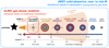 |
Fig. 1 Schematic of chemical evolution on dust grains in protostellar stages, modified from Fig. 1.4 of van’t Hoff (2019) and Fig. 14 of Herbst & van Dishoeck (2009). Ice layers are dominated by different species (e.g., H2O, CO, and COMs) that are denoted in different colors. The typical temperature and density in different evolutionary stages are labeled on arrows in the bottom. The small red box indicates the hot core region where the temperature is high enough (>100 K) to sublimate most of the volatile materials, and therefore the gas-phase molecules can be traced by radio telescopes at (sub)millimeter wavelengths. The big blue box indicates that IR telescopes such as JWST are tracing everything along the line of sight, including ice in the vast envelope and gas in the hot core. |
2 Observations and data reduction
2.1 ALMA
The ALMA data of IRAS 2A and B1-c were taken as part of program 2021.1.01578.S (PI: B. Tabone), which targeted magnetic disk winds of five Class 0 protostars in Perseus and also observed a large number of emission lines of gas-phase COMs. The observations were taken with a combination of an extended configuration, C-6 (θbeam = 0.12″ × 0.09″), and a more compact configuration, C-3 (θbeam = 0.58″ × 0.34″). The maximum recoverable scales (θMRS) for the C-6 and C-3 datasets are 1.6″ and 6.2″, respectively. The data cover nine spectral windows in Band 7 between 333.8 and 347.6 GHz, including one 1.875-GHz wide continuum window with a spectral resolution of 0.87 km s−1. Among the eight line windows, six windows have a spectral resolution of 0.22 km s−1 and a frequency coverage of 0.12 GHz or 0.24 GHz; the remaining two windows are wider (0.48 GHz) but have a lower spectral resolution of 0.44 km s−1.
The data were pipeline-calibrated using CASA versions 6.2.1.7 and 6.4.1.12 (McMullin et al. 2007). The measurement sets from the C-3 and C-6 configurations were combined via concatenation and subsequently continuum subtracted and imaged using the concat, uvcontsub, and tclean tasks in CASA version 6.4.1.12. For B1-c, a briggs weighting of 0.5 was used for all the spectral windows to improve the angular resolution, yielding a synthesized beam of θbeam = 0.08″ × 0.11″ for the 0.88 mm continuum and the spectral windows, which corresponds to a spatial resolution of ~30 au at ~320 pc (i.e., the distance of the Perseus star-forming region). For IRAS 2A, a higher briggs weighting of 2.0 was used to increase the S/N of the H13CO+ line at 348.998 GHz (customized for Nazari et al. 2024b), resulting in a larger beam size of 0.25″ × 0.4″ for that spectral window (336.93–337.05 GHz). The root mean square (rms) is about 1.5–2.0 mJy beam−1 for all the spectral windows except that the one with a larger beam has a higher rms of 5.0 mJy beam−1. The rms for the continuum is about 0.2 mJy beam−1.
2.2 JWST
The JWST/MIRI-MRS data of IRAS 2A and B1-c were taken in the Guaranteed Time Observation (GTO) programs 1236 (PI: M. E. Ressler) and 1290 (PI: E. F. van Dishoeck), respectively, as part of the JWST Observations of Young protoStars+ (JOYS+) collaboration2. MIRI-MRS covers 4.9–27.9 μm with a spectral resolution of R = λ/Δλ of 1300–3700 (Rieke et al. 2015; Wright et al. 2015; Wells et al. 2015; Labiano et al. 2021; Wright et al. 2023; Argyriou et al. 2023). The dither patterns were optimized for extended sources, with the two-point pattern used for IRAS 2A and the four-point pattern for B1-c. Two pointings were observed for B1-c; one centered on the protostar itself, and one covering the blueshifted outflow. Both programs included dedicated background observations in a two-point dither pattern that allow for a subtraction of the telescope background and detector artifacts. All observations were taken using the FASTR1 readout mode and cover the full 4.9–27.9 μm wavelength coverage of MIRI-MRS. The total integration time of 333 s for IRAS 2A was equally divided over the three MIRI-MRS gratings. For B1-c, the total integration time was 8000 s, of which 4000 s were used in grating B (MEDIUM) to get a good S/N in the deep silicate absorption band, and 2000 s each for gratings A (SHORT) and C (LONG).
The data were processed through all three stages of the JWST calibration pipeline version 1.12.5 (Bushouse et al. 2023), using the procedure described by van Gelder et al. (2024). The reference contexts jwst_1126.pmap and jwst_1177.pmap of the JWST Calibration Reference Data System (CRDS; Greenfield & Miller 2016) were used for IRAS 2A and B1-c, respectively. The raw data were processed through the Detector1Pipeline using the default settings. The dedicated backgrounds were subtracted at the detector level in the Spec2Pipeline, and the fringe flat was applied for extended sources (Crouzet et al. in prep.) along with a residual fringe correction (Kavanagh et al. in prep.). An additional bad pixel map was applied to the resulting calibrated detector files using the Vortex Imaging Processing package (Christiaens et al. 2023). The final datacubes were constructed using the Spec3Pipeline for each band of each channel separately.
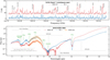 |
Fig. 2 Overview of the ALMA spectra (the continuum spectral window from 333.78 to 335.65 GHz; top panel) and JWST/MIRI-MRS spectra (bottom panel) of NGC 1333 IRAS 2A and B1-c. The JWST spectrum of IRAS 2A between 8.85 and 11.7 μm was binned by a factor of ten for better visualization. In the bottom panel, the fingerprint ranges of COM ices between 6.8 and 8.8 μm are highlight in orange. Important emission lines in the ALMA spectra and absorption bands in the JWST spectra are labeled in each panel. |
3 Methods
3.1 ALMA
The ALMA spectrum of IRAS 2A was extracted from the peak pixel of CH3OH emission at RA 03h28m55.569s, Dec +31d14m36.930s (J2000). This position was selected based on the integrated intensity maps of a dozen of O-COM lines shown in Fig. A.1, which is slightly offset from the continuum peak at RA 03h28m55.5735s, Dec +31d14m36.925s (6 pixels offset in RA and 2 pixels in Dec; the pixel size is 0.01″ × 0.01″). The line emission of IRAS 2A near the continuum peak is attenuated, probably due to the high optical depth of dust in Band 7 (e.g., De Simone et al. 2020). B1-c does not show the same attenuation issue, and therefore its spectrum was extracted from the peak pixel of the continuum emission at RA 03h33m17.881s, Dec +31d09m31.740s, which is consistent with the emission peak of O-COMs (Fig. A.2).
The ALMA spectra of the continuum window (333.78–335.65 GHz) of IRAS 2A and B1-c are shown in the top panel of Fig. 2. The spectra were converted to brightness temperature (K) scale by averaging over the synthesized beam. Line identification and spectral fitting were performed using the spectral analysis software CASSIS3 (Vastel et al. 2015). We mainly considered O-COMs in the fitting, including methanol and its isotopologs (CH3OH, 13CH3OH, and ![Mathematical equation: $\[\mathrm{CH}_3^{18} \mathrm{OH}\]$](/articles/aa/full_html/2024/10/aa50706-24/aa50706-24-eq1.png) ), acetaldehyde (CH3CHO), ethanol (C2H5OH), dimethyl ether (CH3OCH3), methyl formate (CH3OCHO), glycolaldehyde (CH2OHCHO), and ethylene glycol ((CH2OH)2). The local thermal equilibrium (LTE) modeled spectra were fit to the observations, and a best-fit column density (N), excitation temperature (Tex), and line width (full width at half maximum; FWHM) were determined for each species in each source by grid fitting or visual inspection.
), acetaldehyde (CH3CHO), ethanol (C2H5OH), dimethyl ether (CH3OCH3), methyl formate (CH3OCHO), glycolaldehyde (CH2OHCHO), and ethylene glycol ((CH2OH)2). The local thermal equilibrium (LTE) modeled spectra were fit to the observations, and a best-fit column density (N), excitation temperature (Tex), and line width (full width at half maximum; FWHM) were determined for each species in each source by grid fitting or visual inspection.
We adopted the grid-fitting method when a species has more than five clean lines detected (clean means the line is unblended or partially blended and the line profile is still recognizable). For each source and each species, a grid of N, Tex, and FWHM was preset, and each grid point corresponds to an LTE model. The χ2 between the observations and the LTE model was only calculated around the fully unblended lines. The model with the smallest χ2 gave the best-fit parameters. The 2σ uncertainties on N and Tex were estimated from the N-Tex contour plots. The uncertainties of N are usually 30–40% of the best-fit values, and the uncertainties of Tex varies with species.
The grid-fitting method was mainly applied to B1-c. However, most of the emission lines in the IRAS 2A spectrum show double-peaked features, suggesting two velocity components. This makes the blending issue more severe, and hence makes it trickier to perform grid fittings. Instead, we fit the spectrum through visual inspection, which is more flexible in this case. For each species and each velocity component, we first determined the υlsr and FWHM based on several strong and unblended lines, then manually adjusted N and Tex to achieve a better fit between the LTE models and the observed spectrum. All the parameter were fine-tuned once a rough range around the best fit was found. In this way, the uncertainties on N and Tex could not be calculated from contour plots, but were estimated at a level of 20–30%. More details about the fitting strategy for line-rich ALMA spectra can be found in Sect. 3.1 of Chen et al. (2023).
3.2 JWST
The JWST/MIRI-MRS spectrum of IRAS 2A has been presented and analyzed in Rocha et al. (2024). Here, we implemented a similar analysis to B1-c. The B1-c spectrum was manually extracted from the continuum peaks at RA 03h33m17.8959s +31d09m31.8578s, which is only ~0.1″ offset from the ALMA continuum peak at 0.9 mm (see Fig. A.3). The diameter was set to four times the size of the point spread function (PSF) of MIRI-MRS (FWHMpsf = 0.033″ × (λ/μm) + 0.106″; Law et al. 2023); that is, the extraction aperture increases toward longer-wavelength channels. In our COM fingerprint range of interest, the aperture size is ~1.4″ in diameter. An additional 1D residual fringe correction was performed especially to remove the high-frequency dichroic noise in channels 3 and 4 (Kavanagh et al. in prep.). Since the photometric calibration between the bands was accurate enough, the 12 sub-bands were stitched together without any flux adjustment being applied.
Starting from the original extracted spectrum, we required five steps to reach the final goal of determining the column densities of COM ices: fit a global continuum (Sect. 3.2.1), subtract the silicate features (Sect. 3.2.2), fit a local continuum (Sect. 3.2.3), remove the superposed gas-phase lines (which is needed for B1-c but might be skipped for other sources if these lines are weak; Sect. 3.2.4), and decompose the COM fingerprint ranges between 6.8 and 8.8 μm using the lab spectra (Sect. 3.2.5). To calculate the ice column density ratios of COMs with respect to a reference species, we also determined the ice column densities of CH3OH and H2O with a slightly different routine than that for the 6.8–8.8 μm range (see Sect. 3.2.6).
3.2.1 Global continuum
The first step was to fit a global continuum level so that the original spectrum in flux scale (λFλ) could be converted into optical depth (τλ) scale by taking the logarithm between the global continuum and the observed spectrum. The goal of this step is not to derive the origin of the mid-IR continuum emission, but to enable the subsequent comparison with the lab spectra that are measured in absorbance (Absv), which is directly linked to optical depth with a scaling factor of 2.303 (i.e., ln 10):
![Mathematical equation: $\[\tau_\nu=2.303 \times A b s_\nu.\]$](/articles/aa/full_html/2024/10/aa50706-24/aa50706-24-eq2.png) (1)
(1)
We fit a third-order polynomial to the observed spectrum in three ranges: 4.9–5.5 μm at the short-wavelength end, 7.75–7.9 μm around the “bump” between the NH4+ band at 6.8 μm and the silicate band at 9.8 μm, and 27.6–27.9 μm at the long-wavelength end (see Fig. 3a). The flux values in the last two ranges were manually lifted by a factor of 1.3 to leave some space for the red wings of the H2O bending mode at ~6 μm and the silicate band at ~18 μm. Both the fit ranges and the lifting factor of 1.3 were tuned carefully to produce a plausible global continuum. The last range of 27.6–27.9 μm was set to be narrow, since using a wider range will create an increasing feature in the polynomial longward of 20 μm which will introduce some artifacts in the optical depth spectrum that do not match with the supposed silicate features in the next step.
3.2.2 Silicate bands
The second step is to fit and subtract the silicate features at 9.8 and 18 μm. This step removes the contribution from silicates to the COM bands in 8.0–8.8 μm, the CH3OH band at 9.74 μm, and the water libration band at ~13 μm as much as possible. The silicate features may not be fully removed, but the residuals will be further excluded in the next step of local continuum subtraction. We tried fitting with two silicate profiles: the observed spectrum toward the galactic center source GCS 3 (Kemper et al. 2004), and the synthetic silicate spectra of pyroxene (MgxFe1-xSiO3) and olivine (MgFeSiO4) computed by the optool code (Dominik et al. 2021). The GCS 3 and the synthetic silicate spectra were scaled manually to match the optical depth spectrum of B1-c. The fitting criterion is to fit the two silicate bands at 9.8 and 18 μm as well as possible without overfitting any part of the observed spectrum, especially the blue wing of the 9.8 μm band.
Figure 3b shows the fitting results of the silicate features. The GCS 3 profile can be scaled deeper at the 9.8 μm band than the optool mixture of pyroxene and olivine, but leaves non-negligible residuals in the blue wing of the 9.8 μm band (roughly between 8 and 9 μm). This has been seen in previous ice studies (e.g., Boogert et al. 2008) and also our JOYS+ data. The reasons why are still being investigated. The scaling factors of the synthetic silicates, pyroxene and olivine, were tuned manually to achieve the best fit. Pyroxene has a more blueshifted 9.8 μm band than olivine, and its absorbance ratio between the 9.8 and 18 μm bands is higher. The contribution of pyroxene is constrained by the small bump at ~8.5 μm in the observed spectrum (see the blow-up in Fig. 3b), which should not be overfit by the blue wing of the synthetic silicate spectrum. Similarly, olivine has a relatively strong 18 μm band and its scaling factor is constrained by not overfitting the 18 μm band. The synthetic silicate spectrum turned out to fit the B1-c spectrum better than the GCS 3 profile. This, however, may not be the case in general, since the observed silicate bands in independent sources can be quite different from one another. The silicate features in the mid-IR spectra of protostellar sources are worth a thorough investigation that is beyond the scope of this paper. We provide some additional details and relevant discussion in Appendix B.
3.2.3 Local continuum
After subtracting the silicate component from the optical depth spectrum, a local continuum was fit between 6.8 and 8.8 μm to isolate the absorption bands of COM ices from other strong features (e.g., the NH4+ band at 6.8 μm, the red wing of the H2O bending mode at 6 μm, and the leftover silicate features in the previous step; Schutte et al. 1999). Due to the richness of absorption features in this range, continuous absorption-free regions for fitting hardly exist. Instead, a sequence of “guiding points” are set manually at certain locations (e.g., Grant et al. 2023). We fit a seventh-order polynomial to about ten guiding points at positions that were set between two absorption bands or in the middle of a broad band to bridge the guiding points on both sides (see Fig. 3c). Polynomials with lower orders would slightly deviate from some of the guiding points or create artificial features.
Similar to fitting a local continuum, the choice of local continuum is somewhat subjective. Rocha et al. (2024) show in their Section 4.2.4 and Appendix J that the ice column densities of some species can be changed by using a different local continuum. In our case, we traced the local continuum as close to the observed spectrum as possible, so that the ice abundances of the targeted COMs are not likely to be overestimated.
The noise level in the optical depth around the COM fingerprint range was also estimated in this step. A second-order polynomial was fit to a small range between 8.227 and 8.240 μm that is relatively free of emission or absorption features. The noise level was calculated using
![Mathematical equation: $\[\sigma=\sqrt{\frac{\sum_{i=1}^N\left(y_i-\bar{y}\right)^2}{N}},\]$](/articles/aa/full_html/2024/10/aa50706-24/aa50706-24-eq3.png) (2)
(2)
where yi is the polynomial-subtracted optical depth at each channel between 8.227 and 8.240 μm, and ![Mathematical equation: $\[\bar{y}\]$](/articles/aa/full_html/2024/10/aa50706-24/aa50706-24-eq4.png) is the mean of yi. The noise level of the B1-c spectrum was estimated as 2.3×10⁻³ in units of optical depth.
is the mean of yi. The noise level of the B1-c spectrum was estimated as 2.3×10⁻³ in units of optical depth.
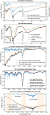 |
Fig. 3 Panels a–d show the four steps to isolate the fingerprint range of COM ices between 6.8 and 8.8 μm from the original JWST/MIRI-MRS spectrum of B1-c: (a) fit a global continuum and convert the spectrum to optical depth scale; (b) subtract silicate features at ~9.8 and 18 μm; (c) trace a local continuum in the 6.8–8.8 μm range to isolate the weak bands of COM ices from other strong features; and (d) trace a baseline of the gas-phase lines in absorption to restore the band profiles of ices. Panel e shows the isolation of the CH3OH ice band at 9.74 μm by tracing a local continuum. The orange-shaded regions in panels a and e show the selected wavelength ranges for the polynomial fitting. |
3.2.4 Gas-phase lines
There are plenty of gas-phase absorption lines superposed on the broad ice bands that need to be accounted for after subtracting the local continuum. An ideal but nontrivial solution would be simultaneously tracing a baseline and fitting LTE models to retrieve the column density and temperature of the gas-phase components. However, deriving the gas properties is not the focus of this paper, so we only considered tracing a baseline of these gas lines to isolate the ice bands that we are interested in. Similar to the local continuum, the baseline was determined by fitting a spline function to a series of guiding points that were set manually (Fig. 3d). The smoothing factor of the spline function was also carefully tuned.
3.2.5 Absorption features of complex organic molecule ices
The final step is to decompose the spectrum between 6.8 and 8.8 μm by fitting with lab spectra of different ices. However, this is not as straightforward as fitting the ALMA spectra where the LTE models can be analytically computed. When fitting the JWST spectra, the variables are not only the temperature and the ice column density of a species (or equivalently, the scaling factor of the corresponding lab spectrum), but also the mixing conditions of the ices. In the solid phase, a species can be mixed with various constituents in different ratios under different temperatures (e.g., CH3OH mixed with H2O in an abundance ratio of 1:10 at 15 K). The relation between the band profile and the mixing condition – that is, mixing constituents, mixing ratio, and temperature – is not linear. Therefore, we need to first select the mixing condition that matches best the observations for each species (which is introduced in this subsection), and then do a least-squares fitting with the selected lab spectra of the candidate species to get a best fit on the ice column densities, or the scaling factors (which will be introduced in the next subsection).
These two steps can be executed either simultaneously or separately. The ENIIGMA code implemented in Rocha et al. (2024) is the first case, which calculates the chi-square of all the possible combinations of lab spectra and searches for the global minimum using genetic algorithms. However, ENIIGMA is limited in the stability of fitting results due to the intrinsic randomness of genetic algorithms. In this work, we performed the two steps of selecting the lab spectra and fitting the scaling factors separately, which can also be used to crosscheck the results reported in Rocha et al. (2024).
Selection of lab spectra. In the first step of this process, we selected a list of species that are likely to contribute to the absorption features between 6.8 and 8.8 μm. These species can be both COMs and simple molecules, and the promising candidates have been explored in Rocha et al. (2024). In this work, we considered 12 molecules in total, including five simple species (CH4, SO2, OCN−, HCOO−, and HCOOH) and seven COMs (CH3CHO, C2H5OH, CH3OCH3, CH3OCHO, CH3COOH, CH3COCH3, and CH3CN). Each species has a collection of lab spectra measured under different mixing conditions of ices (i.e., mixing constituent, mixing ratio, and temperature). The next step is to determine under which mixing condition the lab spectrum matches the observations best. We first did this by superposing all the lab spectra of a certain species on the JWST spectrum to see which one matches the observations best, as is indicated by Figs. 4–5 and C.1, in which each panel shows the comparison between different mixing constituents and temperatures for one species, respectively. For most candidate species, this is already very informative and efficient.
However, if the differences among spectra are small and direct comparison is not straightforward, an alternative way is to compare the peak positions and FWHMs of the characteristic absorption bands of a certain species, when these data are available for the lab spectra (e.g., Boogert et al. 1997; Terwisscha van Scheltinga et al. 2018, 2021; Rachid et al. 2020, 2022). The peak positions and FWHMs of observed bands are derived by fitting Gaussian functions to the observed spectrum. Taking CH3CHO as an example, Fig. 6 shows the comparison between the lab spectra and the observed B1-c spectrum for two CH3CHO bands at ~7.0 (CH3 deformation mode) and ~7.42 μm (CH3 s-deformation and CH wagging modes). It is already straightforward to tell from the left panel that the CH3CHO:H2O mixture fits the observations best. The two panels on the right show that the observed spectrum has both bands obviously wider than the lab spectra, suggesting that these two bands are not only attributable to CH3CHO, but also have contribution from other species. The peak positions of both bands match more closely the H2O mixture than they do the pure ice and the CO mixture, which further supports that the CH3CHO:H2O spectrum is the most suitable one to use in the overall fitting of scaling factors. As for temperature, lower temperatures are favored in the comparison. We chose the spectrum at 15 K for the overall fitting, but 30 K can also be used alternatively, since the difference in band profiles is small under 70 K. The selection of ice mixtures of other species follows the same procedure.
For COMs, there is usually only one mixing ratio that has been measured in laboratories for a specific mixture (e.g., COM:H2O = 1:20), so we can only select among different mixing constituents and temperatures. For some simple species such as CH4, there are more choices for mixing ratios, but within a limited temperature range. Despite the lack of additional laboratory measurements, in Sec. 4.2 we shall show that there is already a lot we can do with the current measurements.
The lab spectra used in comparison had been baseline corrected to isolate the absorption bands of the targeted species from the strong features of the mixing constituents (e.g., H2O and CH3OH). This process is important but sometimes not trivial, especially for the ice mixtures with CH3OH. The details are elaborated in Appendix D.
Overall fitting of the complex organic molecule fingerprint range 6.8–8.8 μm. In the second step, we performed an overall fitting on the scaling factors of all the selected lab spectra (each spectrum corresponding to the best-fit ice mixture of one species), as is described in
![Mathematical equation: $\[\tau_{\mathrm{obs}}=\sum_i^N a_i ~\tau_{i, \mathrm{lab}},\]$](/articles/aa/full_html/2024/10/aa50706-24/aa50706-24-eq5.png) (3)
(3)
where τobs is the observed spectrum between 6.8 and 8.8 μm, and ai is the scaling factor of the i-th component; that is, the selected best-fit lab spectrum of the i-th species. N is the total number of the spectra (or species) that are considered in the fitting. We first performed a normal least-squares fitting to the observations using the Omnifit code(Suutarinen 2015) with all the candidate species taken into account, in order to get a general idea of the best-fit ranges. Then we selected a subgroup of significant candidates for a subsequent Markov chain Monte Carlo (MCMC; Foreman-Mackey et al. 2013) fitting to better constrain the uncertainties on their scaling factors. To reduce the computation time, we set boundaries on the scaling factors to make sure that the fitting results fall in a reasonable range. The lower limits and the initial values were set as zero, and the upper limits were determined by manually comparing the lab spectra with observations (as is done in Figs. 4 and C.2).
3.2.6 Ice bands of CH3OH and H2O
As the simplest and the most abundant COM, CH3OH is usually taken as the reference species to calculate the relative abundances (i.e., ratios) of other COMs. These abundance ratios are generally compared among different sources to see if there are similarities or differences. The abundance of CH3OH ice was derived separately since its strongest mid-IR band is located at 9.74 μm, outside of the 6.8–8.8 μm range. The CH3OH band at 9.74 μm can be isolated by fitting a local continuum on either the original optical depth spectrum (Bottinelli et al. 2010) or the silicate subtracted spectrum. However, the S/N of this band is usually much lower than other parts of the spectrum due to the strong extinction by the silicate 9.8 μm band. Here, we fit a sixth-order polynomial to the original optical depth spectrum in three wavelength ranges: 8.40–8.80, 9.23–9.45, and 10.02–10.40 μm (see Fig. 3d). The local continuum subtracted spectrum between 9.5 and 10.0 μm was then fit by a Gaussian function. We chose to use a Gaussian function instead of the lab spectra for simplicity, since this band is isolated and the fitting results would be similar.
H2O is also a reference species commonly used to calculate relative abundances, especially for simple molecules. We fit the H2O band at 13 μm in the silicate subtracted spectrum using the lab spectra recently measured by Slavicinska et al. (2024). The weaker 6 μm band was taken as a secondary reference. Since this band is very broad and strong, and its spectral profile changes prominently with temperature, it is easy to select the best fitting H2O spectrum to the observations and adjust the scaling factor accurately through visual inspection.
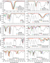 |
Fig. 4 Comparison between the JWST/MIRI spectrum of B1-c (gray) and the lab spectra (colors) in the COM fingerprint range of 6.8–8.8 μm. Each panel focuses on one species and shows the comparison between the observed B1-c spectrum and the lab spectra with different mixing constituents, except for panel c, which shows the lab spectra of HCOO− under different temperatures. The observed spectrum along with the 3σ level is shown in light gray, except for panel a, which blows up the CH4 band at ~7.7 μm, and the observed spectrum is plotted in black for clarity. In each panel, the spectrum in blue corresponds to the pure ice, and the best-fit spectrum to the observations is highlighted with a thicker red line. A similar comparison but for lab spectra under different temperatures is shown in Figs. 5 and C.1. |
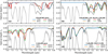 |
Fig. 5 Same as Fig. 4 but for a comparison between different temperatures. Here, we use two species, CH3OCHO and C2H5OH, as examples; the remaining species (CH3CHO, CH3OCH3, and CH3COCH3) are shown in Fig. C.1. The left and right columns show the lab spectra of pure ices and ice mixtures, respectively. In the pure-ice panels, the spectra with crystalline features are highlighted in thicker red lines. The corresponding temperatures indicate the upper limit of crystallines. In the mixed-ice panels, the spectra with the lowest temperature (15 K) are highlighted in thicker blue lines; they are also the spectra used in the overall fitting. |
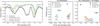 |
Fig. 6 Two methods of selecting the best-fit ice mixture, taking CH3CHO as an example. The left panel shows the direct comparison of spectral profiles between observations and experiments. The middle and the right panels show the comparison of peak position and FWHM of absorption bands between lab spectra and observations. |
3.2.7 Ice column density
Once the best-fit scaling factors are found for the selected lab spectra (for COMs in Sect. 3.2.5), we can calculate the ice column densities of each species by picking a vibrational band, usually the strongest one in the interested wavelength range, and using:
![Mathematical equation: $\[N_{\text {ice }}=\frac{1}{A} \int_{\nu_1}^{\nu_2} a \tau_{\nu, \text { lab }} \mathrm{d} \nu,\]$](/articles/aa/full_html/2024/10/aa50706-24/aa50706-24-eq6.png) (4)
(4)
where A is the strength of this band that extends from wavenumber v1 to v2, τv,lab is the lab spectrum at the wavenumber, v, on the optical depth scale, and a is the scaling factor of this spectrum compared to the observations. In reality, the IR spectra are measured in absorbance (Abs), and the conversion to optical depth is given by Eq. (1). In the cases in which we have used a Gaussian function to represent the absorption band (e.g., for the CH3OH band in Sect. 3.2.6), τv,lab is replaced by the best-fit Gaussian function and the scaling factor, a, is not needed.
4 Results
4.1 ALMA
4.1.1 Emission maps
The continuum emission of IRAS 2A and B1-c appears to be roughly symmetric and round, even at the high angular resolution of ~0.1″ (i.e., 32 au at a distance of 320 pc; see contours in Figs. A.1–A.2), which is consistent with previous observations (Taquet et al. 2015; Segura-Cox et al. 2018; van Gelder et al. 2020; Yang et al. 2021). The COM emission shows consistent morphologies among different species and transitions. In B1-c, the COM emission is symmetric and follows the morphology of the continuum, suggesting that this protostellar system is fairly quiescent. Conversely, the morphologies in IRAS 2A are asymmetric, with the emission attenuated at the continuum peak and stronger at an offset position to the southwest. This asymmetry was not revealed in previous observations with lower angular resolution, and may be related to the dynamics of the protostar and the circumstellar disk (e.g., a recent outburst; Hsieh et al. 2019).
The emission maps of multiple COM lines shown in Figs. A.1–A.2 also reflect how large the hot cores are. The size of a hot core is usually considered as the radius at which T = 100 K, at which temperature most of the volatile species have sublimated from ice mantles into the gas phase. This radius can be estimated analytically with the following equation (Bisschop et al. 2007; van’t Hoff et al. 2022):
![Mathematical equation: $\[R_{\mathrm{T}=100 \mathrm{~K}} \approx 15.4 \sqrt{L / L_{\odot}} \text { au. }\]$](/articles/aa/full_html/2024/10/aa50706-24/aa50706-24-eq7.png) (5)
(5)
Taking the luminosity of 91 and 5.9 L$od for IRAS 2A and B1-c (van Gelder et al. 2022), the RT=100 κ are estimated as 147 au and 37 au (i.e., ~4 and 1 beams), respectively. The spectra of both sources were extracted within RT=100 K; hence, the derived column densities are also expected to be representative of the gas-phase COM abundances inside the hot cores.
4.1.2 Spectra
In the nine spectral windows between 333.8 and 347.6 GHz in ALMA Band 7, rich molecular lines are observed in both sources. We determined column densities (N) and excitation temperatures (Tex) for six O-bearing COMs and one N-bearing COM that have enough clean lines detected; they are CH3OH, CH2DOH, CH3CHO, C2H5OH, CH3OCHO, (CH2OH)2, and CH2DCN. In addition, we detect several strong lines of CHD2OH and CD3OH in both IRAS 2A and B1-c, implying a high deuteration rate of CH3OH in low-mass protostars (e.g., Drozdovskaya et al. 2022), but this will not be studied in this paper.
For other species that are detected but that do not have enough clean lines to constrain N and Tex independently, we provide either upper limits or a range of N assuming Tex = 100–300 K, which is typical for hot cores. These species include the 13C and 18O isotopologs of CH3OH, CH3OCH3, and CH2OHCHO. 13CH3OH only has two strong lines covered in our spectral setup, and they are likely to be optically thick given their high Einstein A coefficients (Aij > 4 × 10⁻⁴ s−1) and the low column density ratio with respect to the main isotopolog. The derived CH3OH/13CH3OH ratios are about 200, larger than the 12C/13C ratio in the vicinity of the Solar System (60–70), which implies that the column densities of 13CH3OH were underestimated due to optically thick lines. It is also difficult to constrain the Tex with both of their upper energy levels Eup > 190 K. Therefore, a lower limit of N is provided for 13CH3OH at the same Tex as the main isotopolog. ![Mathematical equation: $\[\mathrm{CH}_3^{18} \mathrm{OH}\]$](/articles/aa/full_html/2024/10/aa50706-24/aa50706-24-eq8.png) and CH3OCH3 only have weak transitions (Aij<10−6 s−1) covered in our data; therefore, upper limits were estimated assuming a fixed Tex and line width (FWHM) at 3 km s−1. The Tex of
and CH3OCH3 only have weak transitions (Aij<10−6 s−1) covered in our data; therefore, upper limits were estimated assuming a fixed Tex and line width (FWHM) at 3 km s−1. The Tex of ![Mathematical equation: $\[\mathrm{CH}_3^{18} \mathrm{OH}\]$](/articles/aa/full_html/2024/10/aa50706-24/aa50706-24-eq9.png) is fixed at the same value of CH3OH, and the Tex of CH3OCH3 is fixed at 200 K given that the covered transitions have high Eup of > 500 K. CH2OHCHO have ~10 lines detected, but most of them are blended with other stronger lines; thus, its column densities are reported as upper limits as well.
is fixed at the same value of CH3OH, and the Tex of CH3OCH3 is fixed at 200 K given that the covered transitions have high Eup of > 500 K. CH2OHCHO have ~10 lines detected, but most of them are blended with other stronger lines; thus, its column densities are reported as upper limits as well.
Besides CH2DCN, we also detected two N-COMs, NH2CHO and C2H5CN, and each of them have 2–3 strong lines covered in our data. Although these lines are unblended, they share similar Eup and therefore N and Tex are degenerate with each other. In this case, we report N under Tex = 100–300 K. Two 5-atom molecules, ketene (H2CCO) and trans-formic acid (t-HCOOH), each have one strong line detected. They are often studied along with O-COMs given that they may serve as precursors of O-COMs in their formation routes. The column densities of H2CCO and t-HCOOH are also estimated under Tex = 100–300 K because of the degeneracy between N and Tex. Other species, such as the isotoplogs of abundant simple molecules (HDO, HDCO, H13CN), sulfur-bearing molecules (SO, SO2, and their isotopologs), and carbon-chain molecules (HC3N, c- and l-C3H2), also have one or two strong lines detected in the spectra.
The best-fit column densities and excitation temperatures of the aforementioned species along with several other COMs and simple molecules are listed in Table 1. The LTE-modeled spectra along with the observed ALMA spectra of IRAS 2A and B1-c are displayed in Figs. E.1–E.2. The transitions that were considered in the LTE fitting of ALMA spectra are listed in Table L.11
There are two special cases worth mentioning. The first is the determination of the CH3OH column densities. Usually, ![Mathematical equation: $\[\mathrm{CH}_3^{18} \mathrm{OH}\]$](/articles/aa/full_html/2024/10/aa50706-24/aa50706-24-eq10.png) is used to infer the column density of CH3OH assuming a 16O/18O ratio. This is because CH3OH and 13CH3OH tend to be optically thick, and directly fitting their lines may lead to underestimation of their column densities. In our data,
is used to infer the column density of CH3OH assuming a 16O/18O ratio. This is because CH3OH and 13CH3OH tend to be optically thick, and directly fitting their lines may lead to underestimation of their column densities. In our data, ![Mathematical equation: $\[\mathrm{CH}_3^{18} \mathrm{OH}\]$](/articles/aa/full_html/2024/10/aa50706-24/aa50706-24-eq11.png) was not robustly detected, but several CH3OH lines with very high Eup (>1000 K) or very low Einstein A coefficients (Aij ~ 10−7 s−1) were detected. These lines are intrinsically much weaker, and therefore more likely to be optically thin. The column densities of CH3OH were determined based on those high-Eup or low-Aij lines. Our fitting results show column density ratios of
was not robustly detected, but several CH3OH lines with very high Eup (>1000 K) or very low Einstein A coefficients (Aij ~ 10−7 s−1) were detected. These lines are intrinsically much weaker, and therefore more likely to be optically thin. The column densities of CH3OH were determined based on those high-Eup or low-Aij lines. Our fitting results show column density ratios of ![Mathematical equation: $\[\mathrm{CH}_3^{18} \mathrm{OH}\]$](/articles/aa/full_html/2024/10/aa50706-24/aa50706-24-eq12.png) /CH3OH < 0.4% for IRAS 2A and B1-c (Table 1), which are consistent with the expected ratio of 0.18%, assuming 16O/18O~560 in the local interstellar medium (Wilson & Rood 1994).
/CH3OH < 0.4% for IRAS 2A and B1-c (Table 1), which are consistent with the expected ratio of 0.18%, assuming 16O/18O~560 in the local interstellar medium (Wilson & Rood 1994).
The second case is the double-peaked features observed in the emission lines of IRAS 2A, which are not rarely seen in hot cores (e.g., Chen et al. 2023), and probably due to the dynamics of a circumstellar disk (Nazari et al. 2024b). The spectrum can be well fit by two velocity components with different N (and sometimes different Tex and FWHM). By contrast, B1-c only shows one velocity component, even at the continuum peak.
The column densities ratios with respect to CH3OH were calculated to facilitate the comparison with other sources or results in other studies. As famous hot corino sources, IRAS 2A and B1-c have been targeted in previous observations (Taquet et al. 2015; Yang et al. 2021; van Gelder et al. 2020). In particular, the COM ratios in B1-c reported by van Gelder et al. (2020) are consistent with our fitting results within 50% for O-COMs, and even within 10% for CH3CHO and C2H5OH. For IRAS 2A, the COM ratios reported by Taquet et al. (2015) and Yang et al. (2021) are factors of 2–3 higher than our results, which is likely because their angular resolution or sensitivity was not as good as ours (insufficient angular resolution may lead to beam dilution, and insufficient sensitivity would hamper the robust detection of some species).
Column densities and excitation temperatures of gas-phase molecules derived from the ALMA Band 7 spectra.
4.2 JWST
The continuum emission of IRAS 2A and B1-c is spatially unresolved with JWST/MIRI-MRS (as is shown in Fig. A.3 for B1-c); therefore, we only focus on spectral analysis. Studies on COM ices in IRAS 2A have been carried out by Rocha et al. (2024), and here we perform a similar analysis for B1-c.
Based on the selection described in Sect. 3.2.5, we first selected the lab spectra with the mixing conditions that fit best with the observed B1-c spectrum (one spectrum for each candidate species), and then performed overall fittings to constrain the scaling factors of these lab spectra. A certain mixing condition refers to a certain combination of mixing constituent, mixing ratio, and temperature, among which mixing constituent has the most important influence on band profiles. There is limited availability in lab databases of mixing ratios for some species (especially COMs); therefore, we only focus on mixing constituents (Sect. 4.2.1) and temperatures (Sect. 4.2.2).
4.2.1 Constituents of ice mixtures
Figure 4 compares the lab spectra of different mixing constituents with the observations (panels a-j correspond to CH4, SO2, HCOO−, HCOOH, CH3CHO, C2H5OH, CH3OCH3, CH3OCHO, and CH3COCH3). OCN− and CH3COOH are not shown in this figure since they only have lab data for one mixing constituent. CH3CN is also excluded because its three bands between 6.8 and 7.4 μm have very similar profiles among different mixing constituents. The selection of the CH3CN mixture was based on the results of Nazari et al. (2024a), who reported tentative detections of CH3CN ice in the Near Infrared Spectrograph (NIRSpec) data, and the CH3CN:H2O:CO2 mixture is the main contributor of the observed band at 4.43 μm. The comparison between the B1-c spectrum and the lab spectra of OCN−, CH3COOH, and CH3CN ices are shown in Fig. C.2. In the following paragraphs, we introduce the comparison results for each species following the order of display in Fig. 4.
CH4. In B1-c, the CH4 band at 7.67 μm is superposed by gas-phase CH4 lines in absorption, which have been removed before fitting with lab spectra (Sect. 3.2.4). However, none of the existing lab spectra fits perfectly with the observations in terms of peak position. The best two candidates are the H2O mixture with a mixing ratio of 6:100, and a more complex mixture with H2O, CH3OH, and CO2. The 7.67 μm band of these two mixtures is slightly redshifted and blueshifted from the observations, respectively. The same band of the pure CH4 ice and the CH4:H2O (6:10) mixture is more redshifted and too narrow as well. This suggests that in reality the surrounding of CH4 ice is dominated by H2O, and there are also other species present. We finally chose the CH4:H2O (6:100) mixture to fit the observations considering that the mixing ratio of the CH4:H2O:CH3OH:CO2 (1:6:7:10) mixture is not very reasonable (too little H2O and too much CH3OH), but the fitting results are expected to be similar using either of the spectra.
SO2. The 7.6 μm band of the CH3OH mixture fits the blue wing of the observed CH4 band best. Half of this band overlaps with the OCN− band at 7.62 μm, and may lead to degeneracy in the overall fittings (see Sect. 4.2.4).
HCOOH. the H2O mixtures fit the observations better than the pure HCOOH. The difference between the H2O and H2O:CH3OH mixtures at ~8.2 μm is tiny, only that the H2O:CH3OH mixture is slightly redshifted and fits the observed band better. The absorption features shortward of 7.0 μm in the HCOOH:H2O:CH3OH spectrum belong to CH3OH, and was excluded during baseline correction (see Appendix D).
CH3CHO. It has been discussed as an example in Sect. 3.2.5 that the H2O mixture fits the observations best. The 7.0 and 7.42 μm bands of the pure ice and CO mixture deviate from the observations.
C2H5OH. It is a bit hard to select among the pure ice, the H2O mixture, and the CH3OH mixture. The pure C2H5OH matches the observations better at the 7.2 μm band, but its other bands are too wide. The H2O mixture fits better in 6.8–7.2 μm, but its 7.24 μm band is slightly blueshifted from the observations. The CH3OH mixture has similar band profiles to the H2O mixture, but the C2H5OH bands between 6.8 and 7.2 μm are blended with the CH3OH bands, and it is difficult to accurately separated in the CH3OH mixture. We finally chose the C2H5OH:H2O mixture considering that H2O is the dominant species in ice mantles, and the cases for some other O-COMs also show that H2O-rich mixtures suit better than pure ices. The CH3OH is a promising candidate as well, but not selected for technical reasons.
CH3OCH3. Except for the CO mixture, the pure ice and other two mixtures (with H2O and CH3OH) have similar band profiles at 8.59 μm. The H2O has the best match with observations in terms of peak position and band width, while the CH3OH mixture cannot be fully excluded.
CH3OCHO. The mixture with CO, H2CO, and CH3OH fits the observations at 8.1–8.4 μm better than the H2O mixture (panel h of Fig. 4). In the H2O mixture, the C-O stretching band of CH3OCHO at 8.25 μm is significantly blueshifted and smoothed, which does not reproduce the observed profile. This suggests that CH3OCHO is more likely to be formed in a CO-rich environment other than a H2O-rich one. However, a caveat exists that the 8.02 μm band in the lab spectrum of the CH3OCHO:CO:H2CO:CH3OH mixture is mainly contributed by H2CO, not by CH3OCHO. This raises the question how realistic is this mixing ratio between CH3OCHO and H2CO (1:20), considering that the observed 8.03 μm band also likely has a contribution from the CH3COCH3:H2O mixture (panel i of Fig. 4). The relative strength of the H2CO band will affect our estimation on the ice abundance of CH3COCH3. A more detailed discussion on how to deal with the H2CO band blended in the lab spectrum of the CH3OCHO:CO:H2CO:CH3OH mixture is provided in Appendix F.
CH3COCH3. There are more mixtures measured in laboratories than other O-COMs (Rachid et al. 2020), and the comparison is separated into two panels (i and j) in Fig. 4. Panel i shows that the H2O mixture has all the bands blueshifted from the pure ice and the CO or CO2 mixtures. In particular, the CCC asymmetric stretching band is significantly blueshifted from 8.14 to 8.03 μm. The double-peaked CH3 symmetric deformation band at ~7.33 μm is also blueshifted. These blueshifts make the H2O mixture match the observations much better. Panel j shows that the CH3OH mixture has the 8.14 μm band split into two peaks, not matching the observations. The mixture with H2O and CO2 has almost the same spectrum as the H2O only mixture, but the 8.03 μm band is slightly weaker compared to the 7.3 μm band. The weaker 8.03 μm band is favored in the overall fittings since the observed B1-c spectrum tends to be overfit at this position by a combination of H2CO and CH3COCH3 (see Sect. 4.2.3). We finally chose the CH3COCH3:H2O:CO2 (1:10:10) mixture for the overall fittings, but the difference would be small if using CH3COCH3:H2O (1:20).
In summary, our comparison between the lab spectra and the observations reveals that most COM ices (except for CH3OCHO) are surrounded by a H2O-rich environment. For some species such as C2H5OH and CH3OCH3, mixing with CH3OH cannot be ruled out. The possibility of CO-dominated mixtures is low, probably due to its desorption above 20 K. CH3OCHO is an outlier that its surrounding is not dominated by H2O, but rich in CO, H2CO, and CH3OH, implying a formation route of CO hydrogenation. However, this set of mixing constituents (CO+H2CO+CH3OH) is only measured for CH3OCHO; hence, it is too early to conclude that CH3OCHO has a different formation route than other COMs.
4.2.2 Temperature of ice mixtures
Unlike mixing constituents, varying temperature only induces very small differences in band profiles as long as the temperature is below the crystallization point. Figure 5 shows the comparison between the observations and the lab spectra of COM ices under different temperatures. Two species, CH3OCHO and C2H5OH are shown as examples of two scenarios, and the remaining three COMs (CH3CHO, CH3OCH3, and CH3COCH3) are shown in Fig. C.1. For all the considered COMs, the pure ices show significant differences in the band profiles when transiting from amorphous to crystalline state. As temperature increases, the bands become narrower and sharper, some even split into two bands. For some species such as CH3OCHO, the changes in band profiles during this transition are also distinct in the ice mixtures. Because of the dilution of other constituents (e.g., H2O), the band width may remain similar, but the relative intensity or peak position of each band will change significantly after crystallization. On the other hand, the band profiles of C2H5OH:H2O mixture only show small changes after crystallization, which are very difficult to distinguish when compared with observations. The details of other three COMs are described in Appendix C. In general, CH3OCH3 and CH3COCH3 are of the same type as CH3OCHO; and CH3CHO is more like C2H5OH.
By comparing the lab spectra under different temperatures, we can infer the range of crystalline temperature under laboratory conditions (Tcrystal, lab) for pure and mixed COM ices. We also compared the lab spectra with the JWST spectrum of B1-c and constrained the temperature ranges of the detected COM ices (summarized in Table G.1). For pure COM ices, Tcrystal, lab is ≲100 K. Under astrophysical conditions, Tcrystal is usually 20–40% lower. For mixed COM ices, Tcrystal, lab is slightly higher, ≳100 K. Despite noticeable changes in band profiles of crystalline ices, the observations can only constrain the laboratory temperature Tlab of the detected COM ices up to ~100 K (equivalent to 60–80 K in space).
Similar degeneracy is also found for Tlab < 70 K in IRAS 2A using the ENIIGMA fitting code (Rocha et al. 2024). Although IRAS 2A shows evidence of more thermal processing than B1-c by its double-peaked CO2 band at 15.2 μm (e.g., Brunken et al. 2024), the difference in thermal processing is hardly manifested in the band profiles of COM ices. This means that we cannot tell how many COM ices are as cold as 10 K and how many are as warm as 60 K; even if we know, we are still not able to distinguish whether these ices are formed in the cold collapse stage (~ 10 K in space) or the subsequent warm-up stage, since the ices could form in cold environment but then be heated. The only known information is that the observed bands of COM ices are relatively broad and smooth, which is not in favor of the sharp spectral features of crystalline ices. This does not rule out of the presence of crystalline ices, but suggests the observed ices to be mainly amorphous (T < Tcrystal), which is reasonable considering that only a small part of the envelope is heated by the protostar to a temperature as high as Tcrystal.
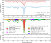 |
Fig. 7 Isolated JWST/MIRI-MRS spectrum between 6.8 and 8.8 μm of IRAS 2A (Rocha et al. 2024) and B1-c (top panel), along with the best-fit decomposition of the B1-c spectrum (bottom panel). The IRAS 2A spectrum was binned by a factor of four, and therefore shows a lower spectral resolution. The B1-c spectrum is the version after removing the gas-phase lines (i.e., the black line in Fig. 3d). In the bottom panel, nine out of 12 candidate species that have statistically significant contribution to the 6.8–8.8 μm range are displayed, with the other three species (SO2, CH3COOH, and CH3CN) excluded. The best-fit mixing conditions (constituents, ratio, and temperature) selected in Sect. 3.2.5 are labeled in the legend. The residue is shown below. A step-by-step version of the best-fit results of the B1-c spectrum is given by Fig. K.11. |
4.2.3 Decomposition of the B1-c spectrum in 6.8–8.8 μm
As introduced in Sect. 3.2.5, after selecting the most suitable ice mixture of each candidate species, we performed least-squares and MCMC fittings to search for the best-fit scaling factors of lab spectra to the observed B1-c spectrum between 6.8 and 8.8 μm. We focus on the spectral decomposition in this subsection, and leave the statistics to the next one. The spectral fitting of the 6.8–8.8 μm range for B1-c is similar to that for IRAS 2A; therefore, our analysis is generally based on the results of Rocha et al. (2024). The top panel of Fig. 7 displays the isolated JWST/MIRI spectrum in the COM fingerprint range (6.8–8.8 μm) of IRAS 2A and B1-c. Despite some difference introduced by the different methods of removing the superposed gas-phase lines, the absorption bands show very similar profiles in these two sources (see elaboration below). The bottom panel of Fig. 7 shows the best-fit results and residues of the B1-c spectrum, and we reserve the statistical details to Sect. 4.2.4.
7.5–7.8 μm. This range mainly contains absorption bands of simple molecules, and therefore is introduced first. The strongest band at 7.67 μm is attributed to the CH4 deformation mode. The residues around this band is due to the deviation of peak position between the observations and the selected lab spectrum, which is the best among the candidates but still not optimal. The blue wing of the CH4 band ~7.6 μm is much weaker in B1-c than in IRAS 2A. It corresponds to one OCN− band and one SO2 band, which overlap with each other by ~50%. The SO2 component is not shown in Fig. 7 since OCN− was favored in the overall fittings by least-squares and MCMC, instead an upper limit was estimated for SO2. There is also a red wing of the CH4 band in IRAS 2A, and is mainly made up of a broad CH3COOH band at ~7.75 μm. This red wing is not present in B1-c after we traced a local continuum that is close to the observed spectrum. Rocha et al. (2024) also discussed in their Sect. 4.2.4 and appendix J that using a different local continuum could remove the CH3COOH component from the overall fit, and CH3COOH is only considered as tentatively detected in IRAS 2A.
6.8–7.5 μm. This range contains four absorption bands at 6.85, 7.02, 7.26, and 7.40 μm. Rocha et al. (2024) attribute them to two O-COMs (CH3CHO and C2H5OH) and HCOO−, which also applies to B1-c. The CH3CHO:H2O mixture is one of the contributors to the 7.02 and 7.40 μm bands. HCOO− has two bands at 7.23 and 7.38 μm, making up the red part of the observed bands at 7.26 and 7.40 μm. C2H5OH has three bands at 6.86, 6.97, and 7.24 μm, of which the contribution is less significant but not negligible.
The peak position of the third band is slightly different between IRAS 2A and B1-c. In IRAS 2A, it is observed to peak at 7.24 μm; more blueshifted than the same band in B1-c which peaks at 7.26 μm. The offset between the HCOO− 7.23 μm band and the observed 7.26 μm band in B1-c leaves an underfit area at 7.3 μm. There are a few candidate species that have absorption bands at around 7.3 μm: CH3CN, CH3COOH, and CH3COCH3. CH3CN has recently been reported to be tentatively detected in NIRSpec spectra of several protostellar sources (Nazari et al. 2024a), but its abundance is mainly constrained by the other two stronger bands at ~6.9 and 7.1 μm, where the absorption is weak in observations. Similarly, the abundance of CH3COOH is constrained by the stronger band at 7.75 μm, which is degenerate with the local continuum subtraction. Even if CH3COOH is present, its 7.3 μm band also tends to be too weak and broad to fill the gap at 7.3 μm in the observed B1-c spectrum. The best candidate turns out to be the H2O-rich mixtures of CH3COCH3, of which the CH3 symmetric deformation band at 7.33 μm can help solve the problem, and the other two bands at 7.03 and 8.03 μm also fit well with the observations (see panel i of Fig. 4). In Rocha et al. (2024), CH3COCH3 is not considered as firmly detected in IRAS 2A based on their recurrence analysis (see their Sect. 4.2.2). A possible explanation is that they trace a local continuum that is not close enough to the observed spectrum when isolating the COM fingerprint range, and therefore leave some space for CH3COOH bands at 7.7 and 7.3 μm. However, if they trace a local continuum close to the observed spectrum as we did, there will also be an unfit area at ~7.3 μm (shown in their Fig. J.2), which can be attributed to CH3COCH3.
7.8–8.8 μm. This range is composed of several blended bands between 7.9 and 8.45 μm and a small band at 8.63 μm. The band at 8.03 μm is contributed and slightly overproduced by a combination of H2CO band at 8.02 μm and CH3COCH3:H2O band at 8.03 μm. The contribution of H2CO was fixed by fitting its another band at 6.67 μm (see Appendix F). To alleviate the overestimation, we chose the CH3COCH3 mixture with H2O and CO instead of the H2O-only mixture, since the H2O:CO2 mixture has a weaker 8.03 μm band (Fig. 4 j), although the difference is small. The broad band peaking at 8.24 μm is composed of the broad HCOOH band at 8.17 μm and the double-peaked CH3OCHO band at ~8.2 μm. The observed band at 8.63 μm matches best with the CH3OCH3:H2O band at 8.6 μm, with potential contribution from the SO2:H2O band at 8.67 μm. Similar to CH3COCH3, CH3OCH3 is also considered as tentative detection for IRAS 2A based on the recurrence analysis; however, this is likely because Rocha et al. (2024) only perform the fittings over 6.8–8.6 μm, missing a large portion of the observed 8.63 μm band. After extending the considered wavelength range to 8.8 μm, CH3OCH3 is likely to be considered as a firm detection (as is shown in Fig. 4g). Besides the contribution of the aforementioned species, there is still an unfit band between 8.3 and 8.4 μm, also seen in other JOYS+ sources. It is recently found to be attributable to CH2OH (priv. comm. with W. Rocha), and will be studied in a future paper. On the other hand, the region at ~8.5 μm is overfit by the CH3 rocking band of CH3OCHO. The reason is unclear, and could be related to the local continuum subtraction.
The decomposition results of the COM fingerprint range between 6.8 and 8.8 μm are generally the same for B1-c (this work) and IRAS 2A Rocha et al. (2024), in spite of different fitting strategies. The only difference is that we tend to consider CH3OCH3 and CH3COCH3 as firmly detected and provide constraints on their ice column densities instead of upper limits (see Sect. 4.2.4).
4.2.4 Fitting statistics
We adopted least-squares and MCMC fittings to find the best-fit values and uncertainties of the scaling factors of lab spectra (see Table I.1). In the least-squares fitting, we considered all the 12 candidate species: CH4, SO2, OCN−, HCOO−, HCOOH, CH3CHO, C2H5OH, CH3OCH3, CH3OCHO, CH3COOH, CH3COCH3, and CH3CN (i.e., N = 12 in Eq. (3)). The scaling factor of H2CO was determined from the band at 6.67 μm, and was fixed when fitting the 6.8–8.8 μm range (see details in Appendix F).
The least-squares fitting results show that the lab spectrum scaling factors of most of the candidate species were well constrained with relative errors smaller than 10% (see Table I.1). There are four exceptions: SO2, CH3OCH3, CH3COOH, and CH3CN, and particularly, SO2 and CH3COOH have very little contribution. The absence of CH3COOH is because we traced a local continuum close to the observed spectrum, which eliminated the red wing of the CH4 band at 7.67 μm. However, the lack of SO2 is more likely because its band at 7.6 μm is too close to the OCN− band at 7.62 μm, and hence highly degenerate with each other. The blue wing of the CH4 band in B1-c is less prominent than in IRAS 2A, making it more difficult to distinguish between the contribution from SO2 and OCN−. The degeneracy origin prevents us from drawing the conclusion that SO2 is not present or more depleted in B1-c than in IRAS 2A. Instead, an upper limit was estimated for SO2 by only scaling the lab spectrum of SO2 to the observations (Fig. 4b). For CH3OCH3 and CH3CN, the best-fit scaling factors are not negligible, but the relative errors are slightly larger than other species, mainly because their bands correspond to weak and blended absorption features in the observations.
In the least-squares fitting, eight out of 12 candidate species have fairly small relative uncertainties (<10%). In the next step, we performed an additional MCMC fitting on these eight species plus CH3OCH3 (i.e., nine species in total) to get a better understanding of the uncertainty level. CH3OCH3 was taken into consideration because it is the main contributor to the observed band at 8.63 μm, and it is one of the most abundant O-COMs observed in the gas phase. We did not include CH3CN in the MCMC fitting since it does not have a characteristic band in the 6.8–8.8 μm range; all the three bands are weak and blended with others. Including CH3CN would also make the MCMC fitting less convergent, suggesting that its contribution is less significant. Instead, we report upper limits for CH3CN like for SO2 and CH3COOH.
The best-fit scaling factors derived from the MCMC fitting are consistent with the least-squares within 5%. Fig. K.21 displays the posterior distributions of each component. Most components are rather independent from each other, except for pairs that have similar band locations (e.g., CH4 and OCN−, HCOOH and CH3OCHO). The relative uncertainties generally increase, but still at a low level of ~10%, except for CH3OCH3, whose relative uncertainty is ~20%. For the left three species, SO2, CH3COOH, and CH3CN, we report only upper limits. We manually scaled the lab spectrum of each species to the observed B1-c spectrum (e.g., Fig. C.2), and the maximum scaling factors allowed by the observations were converted to upper limits of ice column densities.
Based on the fitting results of scaling factors, the ice column densities of each species can be calculated using Eq. (4). The absolute ice column densities are on the same order of magnitude in B1-c (this work) and IRAS 2A (Rocha et al. 2024). The uncertainties of the ice column densities are propagated from scaling factors (~10%), band strengths (~20%), and the steps taken to isolate the COM bands between 6.8 and 8.8 μm (Sects. 3.2.1–3.2.4). The uncertainties of the isolation steps should be dominant but also difficult to quantify, since that they are more or less subjective. Here we estimated a conservative uncertainty level of 50% for isolating the COM fingerprint range, which resulted in a ~55% total uncertainties of the ice column densities. This uncertainty level is consistent with that of IRAS 2A reported in Rocha et al. (2024). The derived ice column densities and uncertainties, along with the temperatures and mixing constituents of the best-fit lab spectra are summarized in Table 2 for both B1-c (this work) and IRAS 2A (Rocha et al. 2024).
Ice column densities of candidate species derived from the least-squares and MCMC fittings to the JWST/MIRI-MRS spectra of NGC 1333 IRAS 2A and B1-c.
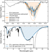 |
Fig. 8 Fitting results of the CH3OH band at 9.74 μm (top panel) and the H20 band at 13 μm (bottom panel). The hatched regions indicate the integrated areas for calculating the ice column densities of CH3OH and H2O. |
4.2.5 CH3OH and H2O bands
The strategies for fitting the CH3OH band at 9.74 μm and the H2O and at 13 μm have been introduced in Sect. 3.2.6. Here we report the fitting results and the derived ice column density of CH3OH and H2O. The CH3OH band at 9.74 μm is isolated and was fit by a Gaussian function (see top panel of Fig. 8). However, it is likely that the best-fit Gaussian function underestimates the real intensity of this band because of the silicate extinction. The extinction correction factor is not trivial to estimate, and a better strategy would be combining the two CH3OH bands in the NIRSpec range (at 3.4 and 3.9 μm) and fit all three bands simultaneously. Unfortunately, the CH3OH band at 3.4 μm is below the detection limit of our observations of B1-c, probably due to the strong extinction by H2O at ~3.05 μm.
The strength of the 3.9 μm band is also not well constrained, since there is strong indication that a grain shape correction is needed to properly trace the continuum of this band (Dartois et al. 2022, 2024). Considering that NIRSpec data are not the focus of this paper and will be reserved for following studies, we performed a preliminary analysis of the 3.9 μm band and derived an upper limit of 4.0×1018 cm−2 for the CH3OH ice column density (see details in Appendix J). For comparison, the best-fit Gaussian to the 9.74 μm band resulted in a column density of 2.0×1018 cm−2. We finally adopted a value of 3.0×1018 cm−2, which corresponds to 1.5 times the best-fit Gaussian. As is shown in the top panel of Fig. 8, this correction factor of 1.5 is reasonable when considering the extinction of the silicate band at 9.8 μm. The uncertainty was estimated as ±1.0 × 1018 cm−2.
The fitting result of the H2O band at 13 μm is shown in the bottom panel of Fig. 8. A scaling factor of 14.5 was estimated through visual inspection for the lab spectrum of H2O ice at 15 K (Sect. 3.2.6), giving a column density of 2.5× 1019 cm−2. The slight excess between 10 and 12 μm is likely due to the over-subtraction of silicate features, as the synthetic silicates have a wider red wing of the 9.8 μm band than the GCS 3 profile (Fig. 3b).
With the ice column densities of H2O and CH3OH derived, we are able to calculate the relative abundances of other species, which are presented in Table 2. The total ice abundance of the detected six COMs, namely CH3OH, CH3CHO, C2H5OH, CH3OCH3, CH3OCHO, and CH3COCH3, is 14.6% with respect to H2O ice in B1-c. As the most abundant COM, the relative abundance of CH3OH is 11.9%, dominates more than 80% of all COMs. The upper limit of the most abundant N-COM, CH3CN, is 1.2% with respect to H2O. According to Rocha et al. (2024), the ice abundances of all the O-COMs and CH3OH with respect to H2O are 9.8% and 6.3% in IRAS 2A, respectively; the upper limit of CH3CN is 1.7%. The ice ratios between CH3OH and other COMs will be discussed in Sect. 5. We provide the statistics but leave out the discussion on the simple species as they are beyond the scope of this study.
5 Discussion
5.1 Column density ratios: Ice versus gas
The detection of COM ices by JWST (this work and Rocha et al. 2024) strongly suggests that the formation of COMs starts in the solid phase, as is illustrated in Fig. 1. However, it remains unclear to what extent the gas-phase chemistry will alter the composition of COMs after their sublimation from dust grains. Now, with COMs observable in both gas and ice, we are able to gain insights into this phase transition by comparing the COM ratios in both phases.
Our comparison is focused on four O-COMs: CH3CHO, C2H5OH, CH3OCH3, and CH3OCHO, which are detectable in both gas and ice. Their ratios with respect to CH3OH in the two phases are summarized in Fig. 9. The number of sources that have COM ice ratios derived is limited. Therefore, in addition to the two case-studied sources IRAS 2A and B1-c, we also include the comet 67P/C-G for comparison, of which the ice abundances of detected molecules are reported in Rubin et al. (2019). For the gas ratios, in addition to previous observations of IRAS 2A and B1-c (Taquet et al. 2015; Yang et al. 2021; van Gelder et al. 2020), we also collected literature data of other sources with different masses and luminosities from previous line surveys (i.e., PILS, PEACHES, and CoCCoA; Jørgensen et al. 2018; Manigand et al. 2020; van Gelder et al. 2020; Yang et al. 2021; Chen et al. 2023), in order to better represent the gas-phase trend using a larger sample. For the PEACHES sources, we adopted the CH3OH column density derived from optically thin minor isotopologs (i.e., 13CH3OH or ![Mathematical equation: $\[\mathrm{CH}_3^{18} \mathrm{OH}\]$](/articles/aa/full_html/2024/10/aa50706-24/aa50706-24-eq44.png) by van Gelder et al. (2022).
by van Gelder et al. (2022).
Figure 9 shows two different cases: CH3OCHO and CH3OCH3 show constant gas-phase ratios among the ALMA sample, which also matches well with the ice ratios. In contrast, CH3CHO and C2H5OH show larger scatter in the gas-phase ratios, and the ice ratios are higher than the gas ones by 1–2 orders of magnitude. The possible reasons are discussed in the following subsections.
5.2 Origin of the similarity in complex organic molecule ratios between ice and gas
The top panels in Fig. 9 show constant gas-phase ratios of CH3OCHO and CH3OCH3 with respect to CH3OH in both low- and high-mass sources, and the good consistency in the ratios between gas and ice. These can be explained by direct inheritance or strong chemical links among CH3OCHO, CH3OCH3, and CH3OH. Direct inheritance means that the bulk of CH3OCHO, CH3OCH3, and CH3OH remain intact during the transition from ice to gas, and their relative abundances also stay on the same level in the gas phase. In the hot core phase, either their absolute abundances remain stable, or their abundances are altered similarly due to a strong chemical link. For instance, they are involved in a similar chemical network and share similar routes of formation and destruction. The numerical simulations on grain-surface chemistry by Simons et al. (2020) suggest that CH3OH and CH3OCHO could share the same precursor (CH3O radical) in their formation pathways. Although CH3OCH3 is not discussed in Simons et al. (2020), studies by Garrod et al. (2022) who present simulation results of a three-phase chemical network (bulk ice, grain surface, and gas phase) show that the CH3O radical plays an important role in the formation of CH3OCH3 ice. The possibility of having chemical links among CH3OH, CH3OCHO, and CH3OCH3 is also supported by the remarkably constant ratio between CH3OCHO and CH3OCH3 observed in a large sample of protostellar sources with different masses and luminosities (Coletta et al. 2020). However, it is difficult to clearly distinguish between the cases of direct inheritance and strong chemical links only by observations; more studies by simulations and experiments are needed to break this degeneracy.
There is also observational evidence that COMs other than CH3OH can be inherited to later stages (e.g., the recent detection in the protoplanetary disk around Oph IRS 48; Brunken et al. 2022; Yamato et al. 2024; Booth et al. 2024). The trend of O-COM abundances in the protoplanetary disks seem to be consistent with those observed in protostars (e.g., there are more CH3OCH3 and CH3OCHO than CH3CHO and C2H5OH in the gas phase), though the exact ratios with respect to methanol are different. Theoretically, the gas-phase COMs observed in the Class 0 stage can be accreted to the circumstellar disk, and some of them will freeze out in the disk midplane at the Class II stage. However, it is not clear to what extent the high temperature environment generated by the accretion shock at the disk-envelope interface would destroy these molecules.
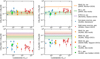 |
Fig. 9 Ratios of four O-COMs with respect to CH3OH in gas (data points) and ice (shaded regions). Gas ratios are collected from a total sample of nine low-mass sources from this work and literature (blue circles; Jørgensen et al. 2018; Manigand et al. 2020; van Gelder et al. 2020; Yang et al. 2021), and 14 high-mass sources from the coccoa survey (Chen et al. 2023). Ice ratios are available for only two protostars (IRAS 2A and B1-c; Rocha et al. 2024, this work) and one comet (67P/C-G; Rubin et al. 2019). All data of the two focused low-mass sources, NGC 1333 IRAS 2A and B1-c, are colored in orange and green, respectively. The gas ratios of IRAS 2A and B1-c derived in this work and previous observations are highlighted in stars and squares (Taquet et al. 2015; van Gelder et al. 2020), respectively. Upper limits are denoted by downward triangles or arrows. |
5.3 Origin of the difference in complex organic molecule ratios between ice and gas
5.3.1 Gas-phase reprocessing
In contrast to CH3OCHO and CH3OCH3, CH3CHO and C2H5OH show not only large scatters in their gas-phase ratios with respect to CH3OH, but also inconsistent ratios between ice and gas (bottom panels in Fig. 9). The large scatter in gas-phase ratios among different sources may be caused by the physical structures (e.g., the presence of a circumstellar disk can lower the temperature in the hot core; Nazari et al. 2022b, 2023). It is also possible that gas-phase chemistry after ice sublimation plays an important role in the chemical evolution of CH3HO and C2H5OH, in which case the variance in physical properties (density, temperature, and UV intensity) are reflected in the chemical abundances. Chen et al. (2023) suggest that C2H5OH may go through gas-phase destruction in the hot core phase. For example, C2H5OH can be H-abstracted by OH radicals or halogen atoms and finally converted into HCOOH, H2CO, and two other O-COMs, CH2OHCHO and CH3COOH (Skouteris et al. 2018). The situation of CH3CHO is more complicated. Simulation results reported by Garrod et al. (2022) show that a significant proportion of CH3CHO is formed in the gas phase, leading to an increasing gas-phase abundance of CH3CHO during the warm-up stage, compared to the ice abundance in the cold collapse stage. However, our observations reveal the opposite case. The CH3CHO ratios with respect to CH3OH are actually lower in gas than in ice by more than one order of magnitude, which implies more CH3CHO is consumed (either destructed into smaller species or converted into larger COMs) than reproduced in the gas phase.
It is not clear to what extent the gas-phase chemistry in hot cores can change the abundances of COMs after they sublimate from dust grains (e.g., Balucani et al. 2015). The influence of gasphase chemistry in the COM abundances can be a few factors or orders of magnitude, and it is likely to vary among different species. Astrochemical models and experiments are required to further investigate the gas-phase chemical network in hot cores.
5.3.2 Spatial distribution
Besides the influence of gas-phase chemistry, it is also important to consider observational effects (e.g., beam dilution). ALMA and JWST are tracing different parts of protostellar systems: ALMA only observes the emission (or absorption) lines of gasphase molecules, mostly from the central hot core region; in comparison, JWST traces materials along the line of sight in a pencil-like beam, and the observed materials can be in both phases, as long as their spectral features fall between 0.6 and 27.9 μm (i.e., the wavelength coverage of NIRSpec plus MIRI). The molecules detected by JWST, in particular those in the solid phase, are mostly coming from the extended envelope instead of the central hot core.
Figure 10 shows how spatial distribution can affect the observed column density ratios between two species. In ALMA observations (top panel of Fig. 10), it is possible to spatially resolve a hot core; that is, the spatial scale corresponding to the beam size is smaller than the region where most of the ice mantles has sublimated into the gas phase. Assume species 1 has higher sublimation temperature than species 2, then its gas material will be present and emit in a more compact region (i.e., within a smaller radius). If the beam size is small enough to resolve the emitting regions of both species 1 and 2, the observed ratio between species 1 and 2 will be representative of the actual ratio. On the other hand, if the beam is not able to resolve the emitting region of any of the species, then its (or their) emission will be diluted within the beam, and the ratio between species 1 and 2 will be underestimated, since the beam dilution effect is more severe for the more compactly distributed species. In the case of our ALMA observations, the angular resolution is ~0.1″, equivalent to ~32 au at the distance of 320 pc for IRAS 2A and B1-c. As already estimated in Sect. 4.1.1 using Eq. (5), the hot core sizes of IRAS 2A and B1-c are 147 au and 37 au, respectively, both spatially resolvable. This means that the gas-phase COM ratios derived from our ALMA data are likely to be free from beam dilution effects.
In JWST observations (bottom panel of Fig. 10) the observed ice column densities of COMs are integrated along the line of sight in the protostellar envelope, and therefore dependent on the spatial distribution of these species. Assume that the ice of species 1 is present in a less extended region in the envelope than species 2. This situation is possible when species 2 starts to form in the solid phase at lower density than species 1 due to different formation mechanisms. Since JWST observes an integrated abundance (i.e., column density) along the line of sight, the integrate is done over a more extended region for species 2, and as a result, the ice column density ratio between species 1 and 2 estimated from JWST observations is lower than the value if we only pick a small region inside the envelope. If species 1 appears to be CH3OH and species 2 corresponds to CH3CHO or C2H5OH, and the resolution of ALMA observations is high enough to resolve the emitting regions of both species, than the ice ratios between CH3CHO (or C2H5OH) and CH3OH estimated from JWST observations will be higher than the gas ratios derived from ALMA observations, as we find in this work.
More quantitatively, we test the influence of spatial distribution on column density ratios between two species with a toy model. We took the 1D spherical model created by Kristensen et al. (2012) for IRAS 2A. The temperature and H2 number density profiles of this model are shown in the top left panel of Fig. 11, with corresponding cartoons shown in the bottom panels. We calculated the H2 column density (i.e., number density integrated over radius) of an envelope where ices are present between an inner and an outer radius (Rin and Rout). For each species, Rin and Rout can be different; Rin is considered as the sublimation boundary of ices, and Rout corresponds to the formation boundary of ices; that is, ices are only present within the envelope. Inside of Rin, ices have sublimated into the gas phase, and outside of Rout, ices have not formed yet. We assumed that the density distributions of all the species (in both gas and ice) are proportional to that of H2, and we compared the H2 column densities of envelopes with different sizes.
Specifically, we considered two cases. In the first case, envelopes have a fixed Rin but different Rout (as is shown in the bottom middle panel of Fig. 11). Rin is fixed as the radius where T = 100 K, and Rout are set as radius where T = 10, 20, ..., and 90 K. These temperatures are also noted as Tform since they by design correspond to the beginning of ice formation. The top middle panel of Fig. 11 shows how the H2 column density N(H2) changes with Rout. As introduced in Sec. 1 and also supported by studies on gas-phase observations (e.g., Coletta et al. 2020; Nazari et al. 2022a; Chen et al. 2023), O-COMs are suggested to start forming in the cold dense pre-stellar phase through CO hydrogenation. According to the constraints on temperature set by the observations (last column in Table G.1), the COM ices must have been formed under 100 K in laboratories, which is equivalent to ~60 K in space. The difference in N(H2) introduced by different Tform is 50–60% (i.e., about a factor of two).
In the second case, we compared N(H2) in envelopes with a fixed Rout but different Rin. This is to study the influence of desorption temperatures (Tdesorb) on ice abundances of different species, as is shown in the right panels in Fig. 11. For the O-COMs that we focused on in the gas-to-ice comparison (i.e., CH3OH, CH3CHO, C2H5OH, CH3OCH3, and CH3OCHO), Tdesorb are similar to each other, about 130–160 K under lab conditions (Fedoseev et al. 2015, 2022), and will be ≳90 K under astrophysical conditions. For some larger COMs such as (CH2OH)2, Tdesorb can be higher up to 200 K under laboratory conditions (equivalent to ~150 K in space). Although the density is higher toward the protostar, the column densities of envelopes with different Rin can only vary by ~40% assuming Tdesorb ~ 90–150 K for O-COMs.
In reality, each species have different Tform and Tdesorb (Rin and Rout, equivalently). In the extreme case, species 1 in Fig. 10 has Tform = 60 K and Tdesorb = 90 K, and species 2 has Tform = 10 K and Tdesorb = 150 K, then the column density of species 2 traced by JWST will be a factor of 4.3 as that of species 1. For CH3CHO and C2H5OH, the difference should be smaller given their similar Tform and Tdesorb, in which case different spatial distributions is not able to fully explain the observed order-of-magnitude difference in the column density ratios with respect to CH3OH between gas and ice. However, all the estimations were based on the assumption that the density distributions of COMs are proportional to that of H2. This may not be true if the formation or evolution mechanisms of COMs are reacting differently to the H2 density as well as the temperature. The details behind the discrepancy cannot be pinned down only by observations, but require more studies on the spatial distribution of COM ices in protostellar envelopes from the side of simulations and experiments.
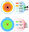 |
Fig. 10 Schematics of how different spatial distributions of two species can affect the column density ratios estimated from ALMA (top) and JWST (bottom) observations. In each panel, two colors are used to indicate two species with different spatial distribution. In reality, the distance between telescopes and sources is very large, and the beam should be like a thin cylinder. For visualization, the beam sizes are exaggerated here. |
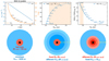 |
Fig. 11 One-dimension model of IRAS 2A and the integrated H2 column densities (top panels), along with the explanatory cartoons (bottom panels). Top left: H2 number density (blue) and temperature (orange) profiles of the physical model of IRAS 2A (Kristensen et al. 2012). Top middle: normalized H2 column densities in envelopes with a fixed inner radius (where T = 100 K) and different outer radii (where T = 10–90 K). Top right: normalized H2 column density in an envelope with a fixed outer radius (the max radius in the model, ~18000 au) and different inner radii (where T = 20–150 K). In the top middle and right panels, each point corresponds to an H2 column density; that is, the integrated H2 number density (top left panel) from an inner radius to an outer one. The orange shaded regions indicate the likely inner or outer radii in real cases. Bottom panels show corresponding cartoons of the toy model. Hot cores and envelopes are colored in red and blue, respectively. In the bottom middle and right panels, yellow arrows indicate the span of envelopes with different outer or inner radii. |
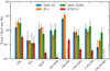 |
Fig. 12 Ice column density ratios of seven species with respect to H2O in three protostars (IRAS 23385, IRAS 2A, and B1-c; Rocha et al. 2024, this work) and one comet (67P/C-G; Rubin et al. 2019). The ice column densities of CH3OH for IRAS 23385 and CH3OCHO for 67P/C-G are not reported in the references. |
5.4 Ice ratios in protostars and comets
Additional to the COM ratios with respect to CH3OH, we also compared the ice column density ratios of simple molecules and COMs with respect to H2O among the three protostellar sources (IRAS 2A, B1-c, and IRAS 23385; Rocha et al. 2024) and the comet 67P/C-G (Rubin et al. 2019). We find similar results to those in Rocha et al. (2024) that the ice ratios of most species with respect to H2O in protostars are similar and generally higher than the comet, except for SO2 (Fig. 12). The COM ratios match better between protostars and the comet when they are calculated with respect to CH3OH instead of H2O (Fig. 9). This may suggest different evolution pathways between simple molecules and COMs, but more sources and studies are needed to draw robust conclusions.
6 Conclusions
We studied COMs and several simple molecules in both the gas and solid phases for two low-mass protostars, NGC 1333 IRAS 2A and B1-c. We derived the column densities in gas and ice by fitting the gas emission lines in the ALMA Band 7 spectra and the ice absorption bands in the JWST/MIRI-MRS spectrum, respectively. We made the first direct comparison in the column density ratios of four O-COMs with respect to CH3OH between the gas and ice, which helps us gain a better understanding of the chemical evolution of these molecules in protostellar systems. Our main conclusions are:
We derived the gas-phase COM column densities for B1-c and IRAS 2A using a set of high-resolution ALMA Band 7 data, and the COM ratios with respect to CH3OH are consistent with previous studies within a factor of two. A small difference may be introduced by the lower spatial resolution and sensitivity in previous observations.
Ices of COMs and other simple molecules were detected in the JWST/MIRI-MRS spectrum of B1-c, following the detection in NGC 1333 IRAS 2A and IRAS 23385+6053 (Rocha et al. 2024). We constrained the total abundance of the detected COM ices with respect to H2O ice, Nice(COM)/Nice(H2O), as ~15%. In particular, CH3OH is the dominate species, with Nice(CH3OH)/Nice(H2O) ~ 12%. The upper limit of the most abundant N-COM, CH3CN, is estimated as Nice(CH3CN)/Nice(H2O) < 1.2%;
By directly comparing the lab spectra of different COM ice mixtures and the observed JWST spectrum of B1-c, we find that most COM ices are likely present in a H2O-rich environment. For some COMs such as CH3OCH3, CH3OH-rich mixtures cannot be ruled out. CH3OCHO is special case in that its H2O-rich mixture matches the observations worse than the CO:H2CO:CH3OH mixture, which implies a formation route of CO hydrogenation;
The temperature of COM ices cannot be well constrained by the observations, since the band profiles of COM ices are highly degenerate before crystallization, which usually occurs at around 100 K under laboratory conditions (~60–80 K in space). For mixed ices of some COMs such as C2H5OH, the degeneracy remains even after crystallization;
The fitting results of the COM fingerprint range (6.8–8.8 μm) using least-squares and MCMC for B1-c are similar to those reported in Rocha et al. (2024) for IRAS 2A and IRAS 23385 using genetic algorithms. The derived column densities and uncertainties are consistent between B1-c and IRAS 2A. The only difference is that CH3OCH3 and CH3COCH3 are considered to be firmly detected in B1-c, but only tentatively detected in IRAS 2A. We expect to further confirm the detection of these COMs in a larger sample;
The comparison of COM ratios with respect to CH3OH between gas and ice shows two cases: CH3OCHO and CH3OCH3 have consistent ratios in both phases, while the ice ratios of CH3CHO and C2H5OH are higher than the gas ones by about one order of magnitude;
The consistency in COM ratios between gas and ice suggests a direct inheritance from ice to gas, and probably a common formation history for CH3OCH3, CH3OCHO, and CH3OH ices. On the other hand, the difference in COM ratios between gas and ice implies the participation of gasphase chemistry after ices sublimate in hot cores. Another possible but less dominant cause is the different spatial distributions of COM ices in protostellar envelopes, which are related to the formation time and desorption temperatures of each species.
Thanks to the successful operation of JWST and the high-quality mid-IR spectra it provides, it is now becoming feasible to have robust detections and quantitative analyses of COMs in the solid phase, allowing direct comparison to the gas-phase counterparts that have been intensively studied by ALMA and other telescopes. As JWST opens a new door to the ice world, it is both intriguing and important to connect it with the already well-explored gas world. The pilot study of two famous hot corinos has shed some light on how COMs evolve through the transition from ice to gas, from the cold envelope to the hot core region. We look forward to further verifying our hypotheses in a larger sample, and additional interpretations from simulation or laboratory studies are highly welcome.
Data availability
Appendices K and L are available on Zenodo at https://doi.org/10.5281/zenodo.13315555
Acknowledgements
This paper makes use of the following ALMA data: ADS/JAO.ALMA#2021.1.01578.S. ALMA is a partnership of ESO (representing its member states), NSF (USA) and NINS (Japan), together with NRC (Canada), MOST and ASIAA (Taiwan), and KASI (Republic of Korea), in cooperation 74 with the Republic of Chile. The Joint ALMA Observatory is operated by ESO, AUI/NRAO, and NAOJ. This work is also based on observations made with the NASA/ESA/CSA James Webb Space Telescope. The data were obtained from the Mikulski Archive for Space Telescopes at the Space Telescope Science Institute, which is operated by the Association of Universities for Research in Astronomy, Inc., under NASA contract NAS 5-03127 for JWST. These observations are associated with program #1290. Astrochemistry in Leiden is supported by the Netherlands Research School for Astronomy (NOVA), by funding from the European Research Council (ERC) under the European Union’s Horizon 2020 research and innovation programme (grant agreement no. 101019751 MOLDISK), by the Dutch Research Council (NWO) grants TOP-1 614.001.751 and 618.000.001, and by the Danish National Research Foundation through the Center of Excellence 81 “InterCat” (grant agreement no.: DNRF150). The work of M.E.R. was carried out at the Jet Propulsion Laboratory, California Institute of Technology, under a contract with the National Aeronautics and Space Administration (80NM0018D0004). H.B. acknowledges support from the Deutsche Forschungsgemeinschaft in the Collaborative Research Center (SFB 881) “The Milky Way System” (subproject B1). P.J.K. acknowledges support from the Science Foundation Ireland/Irish Research Council Pathway programme under Grant Number 21/PATH-S/9360. L.M. acknowledges the financial support from DAE and DST-SERB research grants (SRG/2021/002116 and MTR/2021/000864) of the Government of India. T.H. acknowledges support from the ERC grant no. 832428 Origins.
Appendix A Images of ALMA and JWST observations
Figures A.1–A.2 display the integrated intensity maps (i.e., moment 0 maps) of 12 COM lines in IRAS 2A and B1-c. Five lines are from CH3OH with different upper energy levels (Eup) and Einstein A coefficients (Aij). For the other seven O-COMs, the strongest unblended line of each species was selected to display. Figure A.3 shows the continuum images in 12 MRS channels along with the extracted spectrum.
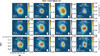 |
Fig. A.1 Integrated intensity maps (i.e., moment 0 maps) of 12 emission lines of eight O-COMs in NGC 1333 IRAS 2A. The quantum numbers, Eup, Aij of each transition are labeled in white text. The contours in light purple indicate the continuum emission at the 30, 50, 100, 200, 300, 400, and 500σ levels (σ = 0.2 mJy beam−1). The beam size (0.1″ × 0.15″) is denoted by white ellipses in the lower right, and the pixel where the spectrum was extracted is marked by a green cross in each panel. The beam size in the fifth panel is slightly smaller (0.08″ × 0.11″), since this transition lies in a different spectral window than the others. |
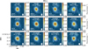 |
Fig. A.2 Same as Fig. A.1 but for B1-c. The continuum contours are set at 3, 5, 10, 20, 30, and 40σ levels (σ = 2 mJy beam−1). |
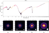 |
Fig. A.3 Extracted spectrum (top) and the continuum images (bottom) of JWST/MIRI-MRS observations of B1-c. Top panel: JWST/MIRI-MRS spectrum of B1-c extracted from the reduced datacubes. The spectrum slices of three sub-bands in each of the four MIRI-MRS Channels are distinguished in three different colors. Bottom panels: continuum images in four Channels (1: 4.9–7.65 μm; 2: 7.51–11.7 μm; 3: 11.55–17.98 μm; 4: 17.7–27.9 μm). The sizes of the PSF and the aperture for spectrum extraction increase as a function of wavelength, and are denoted by white circles, respectively. The extraction position of the ALMA spectrum (also the continuum peak) in Fig. A.2 is marked here using the same green cross. The ALMA extraction position is well within the MIRI apertures, and the small offset to the aperture center is likely due to the lower accuracy of the JWST pointing. |
Appendix B The silicate features
All the silicate spectra used to fit the observed spectrum of B1-c in Sect. 3.2.2 have no features shortward of 7.6 μm. The GCS 3 silicate spectrum shown in Fig. 3b is a smoothed version of the original spectrum, in which the emission and absorption lines that are not attributed to silicates were removed (see the left panel of Fig. B.1).
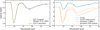 |
Fig. B.1 Silicate spectra between 5 and 30 μm. Left panel: original and smoothed silicate spectra of GCS 3. Right panel: computed spectra of olivine (blue) and pyroxene (orange) with increased grain size or mass fraction of carbon (dashed). |
When fitting the silicate features, we primarily focused on whether the profiles of the 9.8 and 18 μm bands and their optical depth ratios match between the observations and the silicate spectra used for fitting. Figure B.1 shows that the optical depth ratio between the two bands in the GCS 3 profile is ~3.3, larger than those of the computed spectra of olivine and pyroxene (≲ 2). However, the relative intensity of the 18 μm band in the pyroxene spectrum can be reduced by increasing the mass fraction of carbon. The computed spectrum of pyroxene is by default made up of Mg0.7Fe0.3SiO3 and mixed with carbon in a mass fraction of 87% and 13%, respectively. We finally used the spectrum of 80% pyroxene mixed with 20% carbon to get a better fit for the 18 μm band. The 18 μm band in the olivine spectrum can also be widened by increasing the grain size (right panel of Fig. B.1). In Sect. 3.2.2 we only came up with a plausible fitting of the silicate features, but potentially there is a huge parameter space to explore.
Another caveat is that even small difference in the global continuum fitting (Sect. 3.2.1) can change the spectral profile at long wavelengths, which makes it degenerate to fit the global continuum and the 18 μm silicate band. Fortunately, our analysis on the COMs fingerprints between 6.8 and 8.8 μm is little affected by the fitting of the 18 μm band, and we are safe to proceed with a plausible fitting shown in Fig. 3b.
Appendix C Selection of ice mixtures
Figure C.1 is the same as Fig. 5 but shows the temperature comparison for the lab spectra of CH3CHO, CH3OCH3, and CH3COCH3. Same as C2H5OH and CH3OCHO, the band of pure ices will become significantly sharper after crystallization. For the mixed ices, the bands of CH3CHO:H2O mixture become narrower as temperature increases, but the peak positions remain similar and cannot be ruled out by the observations. The major change of CH3OCH3:L2O mixture is the peak position of the 8.63 μm band. The band is blueshifted as temperature increases, and anti-correlates with the observations when T > 120 K. For CH3COCH3:H2O mixture, as temperature increases, the two band at 7.3 and 8.03 μm are redshifted, and the latter splits into two bands. The anti-correlation occurs at 7.3 μm when T >70–90 K.
Appendix D Baseline correction of lab spectra
The lab spectra of COMs mixed with H2O or CH3OH require baseline correction to isolate the weak COM bands from the strong H2O band at 6 μm or the CH3OH band at 6.75 μm. A polynomial was fit to wavelength regions that are free of absorption bands. The baseline correction was only applied between ~6.0 and 10.0 μm, considering that we only fit the observation between 6.8 and 8.8 μm.
For H2O-rich mixtures, the baseline is just the red wing of the H2O bending mode at 6.0 μm, and it is easy to select and fit a polynomial to those ranges that do not have absorption features of the interested species, as is shown in the left panels of Fig. D.1.
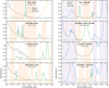 |
Fig. D.1 Baseline correction to lab spectra of ice mixtures. In the left panels, we take the H2O-rich mixtures of CH4 and three O-COMs (CH3CHO, C2H5OH, CH3OCH3) as examples. The original and the corrected spectra are plotted in solid blue and green, respectively. The polynomial is plotted in dashed orange, and the wavelength ranges that were selected to fit the polynomial are highlighted in orange panels. The right panels are similar to the left ones but for CH3OH mixtures. SO2, HCOOH, C2H5OH, and CH3OCH3 are taken as examples. The purple-shaded regions indicate the frequency ranges of CH3OH bands. |
However, it is usually not straightforward to do baseline correction for CH3OH-rich mixtures, especially in 6.5–7.3 μm where there is a CH3OH band with wavy features (see right panels of Fig. D.1; the feature shown in the top panel are CH3OH-only). If the interested species has no overlapping band with CH3OH (e.g., SO2), the routine is the same as for H2O-rich mixtures, except that a higher order polynomial may be needed. Unfortunately, most O-COMs have weak bands around 7.0 μm, and it is difficult to isolate those features from the uneven CH3OH features. We tried to reserve the weak bands between 7.1 and 7.3 μm where the CH3OH spectrum is still smooth and it is feasible to trace a local continuum; this was done for HCOOH and C2H5OH which have a weak band at ~7.2 μm. For those bands shortward of 7.1 μm, we discard them in the corrected spectra (e.g., for C2H5OH, CH3OCH3, and CH3OCHO).
Appendix E Fitting results of the ALMA spectra of IRAS 2A and B1-c
Figures E.1–E.2 show the full ALMA spectra of IRAS 2A and B1-c and the best-fit LTE models of the detected COMs, respectively. Important strong lines of simple molecules are labeled in gray text.
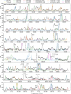 |
Fig. E.1 Best-fit LTE models overlaid on the observed ALMA spectrum of IRAS 2A. |
Appendix F H2CO bands in the CH3OCHO mixture
As was mentioned in Sect. 4.2.1 and shown in Fig. 4h, the lab spectrum of CH3OCHO mixed with CO, H2CO, and CH3OH in a mixing ratio of 1:20:20:20 (hereafter CO-rich mixture) fits the observations best. However, the band at 8μm does not appear in the pure ice and other ice mixtures with H2O and CH3OH, suggesting that this absorption feature comes from neither CH3OCHO nor CH3OH. In fact, this 8μm band belongs to H2CO. Figure F.1 compares the lab spectra of pure H2CO, pure CH3OCHO, and the CO-rich mixture of CH3OCHO under 15 K and 80 K. It is shown that the 8 μm band in the CO-rich mixture remains almost the same as in the pure H2CO, which implies that this band is not affected by ice mixing, and therefore can be treated separately from the CH3OCHO band at 8.25 μm.
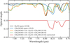 |
Fig. F.1 Comparison between the lab spectra of pure H2CO ice (black), pure CH3OCHO ice (blue), and CH3OCHO:CO:H2CO:CH3OH mixture under 15 K (orange) and 80 K (dashed green). The corrected spectrum for the CH3OCHO mixture under 15 K (red) is plotted at an offset place. |
The problem of using the original lab spectrum of the CH3OCHO:CO:H2CO:CH3OH mixture is that the mixing ratio between CH3OCHO and H2CO is fixed at 1:20, and therefore the intensity ratio between the CH3OCHO band at 8.25 μm and the H2CO band at 8.02 μm is fixed as well. The lab spectra of the CH3OCHO:CO:H2CO:CH3OH mixture at 80 K also shows that the intensity ratio between the 8.25 μm and 8.02 μm bands would increase as part of H2CO has sublimated from the ice mixture at 80 K. However, the 1:20 ratio between H2CO and CH3OCHO may not be realistic; it was found in test fittings that the 8.02 μm band would be overfit and the 8.25 μm band would be underfit the observations if we used the original lab spectrum. As a result, we wanted to break the correlation between H2O and CH3OCHO in the CO-rich mixture to achieve a better fit at both bands.
To address this problem, we fit a Gaussian to the H2CO band at 8.02 μm and subtracted it from the lab spectrum of the CH3OCHO:CO:H2CO:CH3OH mixture, in order to isolate the CH3OCHO band from the H2CO band. There is also a weaker band of H2CO at 8.48 μm, which splits the 8.59 μm band in pure CH3OCHO into two peaks at 8.38 and 8.55 μm in the CO-rich mixture. The presence of H2CO also increase the relative intensity between the bands at 8.55 μm and 8.25 μm from 0.73 (in pure CH3OCHO) to 1 (in CO-rich mixture). To further separate the influence by H2CO, we scaled down the relative intensity of the 8.55 μm band back to 0.73. Finally, we removed other weak feature shortward of 7.8 μm that are either absent in the pure CH3OCHO spectrum or blended with CH3OH features at ~6.9 μm (considering that the ratio between CH3OCHO and CH3OH is 1:20, the contribution from CH3OCHO is negligible). The corrected lab spectrum of the CH3OCHO:CO:H2CO:CH3OH mixture is shown in Fig. F.1, and was the one that used in the overall fitting.
On the other hand, the 8.03 μm band observed in the B1-c spectrum has contribution from not only H2CO, but also H2O-rich mixtures of CH3COCH3 (Sect. 4.2.1 and panels i-j in Fig. 4). To determine how much H2CO accounts for this band, we turned into another characteristic band of H2CO at 6.67 μm, which is outside of the COM fingerprint range. We first fit a local continuum following a similar routine to Sect. 3.2.3 to isolated this band (but without removing the gas-phase absorption lines), and then manually scaled the lab spectra of pure H2CO and the CH3OCHO:CO:H2CO:CH3OH mixture to the observations (see Fig F.2). The observed H2CO band at 6.67 μm is about 0.02 μm blueshifted from pure H2CO, but matches the CH3OCHO:CO:H2CO:CH3OH mixture well (where CO:H2CO:CH3OH = 1:1:1), which implies that H2CO is likely to have surroundings rich in CO and CH3OH in interstellar ices. The two H2CO-relevant lab spectra were scaled to have the same intensities at 6.67 μm. The scaling factor of pure H2CO was then determined by visual inspection, and was fixed in the overall fitting. The ice column density of H2CO was calculated from the 8.02 μm band.
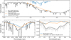 |
Fig. F.2 Isolation of the CH3OCHO bands from the H2CO band in the lab spectrum of the CH3OCHO:CO:H2CO:CH3OH mixture. Top panel: H2CO band at 6.67 μm (blue) isolated by tracing a local continuum (orange) to the observed spectrum (black); superposed gas-phase absorption lines of H2O are not removed here. Bottom-left panel: lab spectra of pure H2CO ice (blue) and the CH3OCHO:CO:H2CO:CH3OH mixture (orange) manually scaled to the isolated H2CO band at 6.67 μm in observations (black). Bottom-right panel: same as the middle panel but for a different wavelength range (7.9–8.5 μm). |
Appendix G Temperature analysis of COM ices
Table G.1 summarizes the temperature-relevant information of the lab spectra of the five O-COMs that are considered detected in the JWST spectrum of B1-c.
Inferred range of crystallization temperature of COM ices under laboratory conditions (Tcrystal,lab). All the considered lab spectra of the five COM ices are obtained from the LIDA database (Rocha et al. 2022).
Appendix H Band strengths
The band strength A describes how strong is the absorbance of a specific band given a unit of ice column density (cm−2). In Table 2, Col. 3 lists the characteristic absorption bands of the species (Col. 1), and Cols. 3–4 provide values and references of the corresponding band strengths. Most of these values and references are the same as those given in Rocha et al. (2024), except for the following species:
CH3OH: for the 9.74 μm band, we adopted A = 1.56 × 10⁻¹⁷ cm−2 from Luna et al. (2018), instead of 1.8 × 10⁻¹⁷ cm−2 from Bouilloud et al. (2015), considering that the former one is more updated.
CH3OCH3: the band strength of the 8.59 μm band is adopted from Table 1 in Terwisscha van Scheltinga et al. (2018), and A is corrected for the H2O mixture by a factor of ~0.5. This factor, known as the relative band strength, is not directly provided in Terwisscha van Scheltinga et al. (2018) but can only be read from the lower right panel of Fig. C.11 therein. Rocha et al. (2024) considered it as 0.5, and the corrected A is 4.9 × 10⁻¹⁷ cm−2. However, a more accurate estimation of this factor would be 0.56–0.57, yielding a slightly larger A of 5.55 × 10⁻¹⁷ cm−2.
CH3COCH3: the band strength of the 7.33 μm band is originally measured as 1.39 × 10⁻¹⁷ cm−2 by Hudson et al. (2018). The relative A of the H2O mixture is not directly stated, but plotted in the lower right panel of Fig. A.11 in Rachid et al. (2020). The estimated relative A is 0.73, and the corrected A is 1.02 × 10⁻¹⁷ cm−2, a bit smaller than 1.2×10⁻¹⁷ cm−2 used by Rocha et al. (2024)4
Appendix I Statistics of fitting the JWST/MIRI-MRS spectrum of B1-c
Table I.1 lists the statistics of fitting the JWST/MIRI-MRS spectrum of B1-c, including the best-fit values and uncertainties of the scaling factors of the selected lab spectra.
Fitting statistics of the scaling factors† of lab spectra. The best-fit values, standard errors (σa) and relative errors (a/σa) are listed for least-squares and MCMC fittings. All the 12 candidate species were considered in the least-squares fitting, and nine of them were included in the MCMC fitting.
Appendix J The CH3OH band at 3.9 μm
To better quantify the ice column density of CH3OH, we checked the 3.9 μm CH3OH band falling in the wavelength coverage of NIRSpec. The NIRSpec integral field unit (IFU) observations of B1-c were taken as part of GTO 1290 in a four-point dither pattern. Details on the reduction of NIRSpec data and the spectra extraction will are not the focus of this work and will be introduced in future publication.
As is shown in the top panel of Fig. J.1, the 3.9 μm band is next to the strong CO2 band at 4.27 μm, of which the blue wing tends to be warped by grain scattering and may need grain size correction (Dartois et al. 2022, 2024). We tried fitting a 3rd-order polynomial to the observed NIRSpec spectrum in 3.72–3.8 μm and 4.17–4.2 μm. This local continuum is only considered as a preliminary analysis without a proper grain shape correction, and it is deviating from the observations longward of 4.2 μm. The observed spectrum between 3.72 and 4.2 μm was converted to optical depth scale by taking a logarithm with the local continuum.
The absorption features in this range were attributed to CH3OH, H2S, and HDO (Slavicinska et al. 2024, the HDO feature will be discussed in a future paper). The CH3OH band was fit by a lab spectrum of CH3OH:H2O (1:1) ice mixture, recently measured by Slavicinska et al. (2024). The contribution of H2S is represented by a Gaussian function. We performed a least-squares fitting on the scaling factor of the CH3OH:H2O spectrum and the coefficients of the Gaussian function (best-fit results displayed in the bottom-left panel of Fig. J.1). The ice column density of CH3OH was then calculated using Eq. 4, where a band strength of 1.56×1017 cm−2 (Luna et al. 2018) was taken. The best-fit scaling factor of the 3.9 μm CH3OH band in the observed NIRSpec spectrum yields an ice column density of 4.0×1018 cm−2 for CH3OH. We scaled the CH3OH:H2O lab spectrum using the same factor as in the middle panel and compared it with the observed MIRI-MRS spectrum at 9.74 μm (the bottom-right panel of Fig. J.1). The lab spectrum overestimates the observed 9.74 μm band, but within a reasonable extent considering the extinction by the silicate band at 9.8 μm.
As was mentioned in Sect. 4.2.5, we finally adopted a CH3OH ice column density of 3.0×1018 cm−2, corresponding to 1.5 times the best-fit Gaussian to the observed 9.74 μm band (top panel in Fig. 8). This result is based on the Gaussian fitting to the 9.74 μm band, with silicate extinction taken into account. The difference between the ice column densities derived from fitting the 3.9 μm and the 9.74 μm bands is small (~30%), suggesting that both the estimations are reasonable. However, considering that the analysis of the NIRSpec spectrum was only preliminary, the result of 4.0×1018 cm−2 was not adopted, instead it was used as a reference to constrain the uncertainty of our fitting results to the 9.74 μm band (σ=1.0×1018 cm−2).
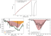 |
Fig. J.1 Fitting of the CH3OH bands at 3.94 and 9.74 μm. Top panel: the NIRSpec IFU spectrum of B1-c (solid black) and the local continuum of the 3.94μm CH3OH band fit by a 3rd-order polynomial (dashed red). Bottom-left panel: best-fit results of the observed absorption complex between 3.75 and 4.03 μm (black, the same as in the top panel but in optical depth scale). The shaded regions in red and yellow correspond to the CH3OH and H2S components, respectively. The overall best-fit spectrum is shown in dashed green. Bottom-right panel: the observed 9.74 μm band in the MIRI-MRS spectrum (black) overlaid with the CH3OH:H2O lab spectrum (red) scaling with the same factor as in the middle panel. |
References
- Argyriou, I., Glasse, A., Law, D. R., et al. 2023, A&A, 675, A111 [NASA ADS] [CrossRef] [EDP Sciences] [Google Scholar]
- Bacmann, A., Taquet, V., Faure, A., Kahane, C., & Ceccarelli, C. 2012, A&A, 541, L12 [NASA ADS] [CrossRef] [EDP Sciences] [Google Scholar]
- Baek, G., Lee, J.-E., Hirota, T., Kim, K.-T., & Kim, M. K. 2022, ApJ, 939, 84 [NASA ADS] [CrossRef] [Google Scholar]
- Balucani, N., Ceccarelli, C., & Taquet, V. 2015, MNRAS, 449, L16 [Google Scholar]
- Bisschop, S. E., Jørgensen, J. K., van Dishoeck, E. F., & de Wachter, E. B. M. 2007, A&A, 465, 913 [NASA ADS] [CrossRef] [EDP Sciences] [Google Scholar]
- Boogert, A. C. A., Schutte, W. A., Helmich, F. P., Tielens, A. G. G. M., & Wooden, D. H. 1997, A&A, 317, 929 [NASA ADS] [Google Scholar]
- Boogert, A. C. A., Pontoppidan, K. M., Knez, C., et al. 2008, ApJ, 678, 985 [Google Scholar]
- Boogert, A. C. A., Gerakines, P. A., & Whittet, D. C. B. 2015, ARA&A, 53, 541 [Google Scholar]
- Booth, A. S., Temmink, M., van Dishoeck, E. F., et al. 2024, AJ, 167, 165 [NASA ADS] [CrossRef] [Google Scholar]
- Bottinelli, S., Boogert, A. C. A., Bouwman, J., et al. 2010, ApJ, 718, 1100 [NASA ADS] [CrossRef] [Google Scholar]
- Boudin, N., Schutte, W. A., & Greenberg, J. M. 1998, A&A, 331, 749 [NASA ADS] [Google Scholar]
- Bouilloud, M., Fray, N., Bénilan, Y., et al. 2015, MNRAS, 451, 2145 [Google Scholar]
- Brunken, N. G. C., Booth, A. S., Leemker, M., et al. 2022, A&A, 659, A29 [NASA ADS] [CrossRef] [EDP Sciences] [Google Scholar]
- Brunken, N. G. C., Rocha, W. R. M., van Dishoeck, E. F., et al. 2024, A&A, 685, A27 [NASA ADS] [CrossRef] [EDP Sciences] [Google Scholar]
- Bushouse, H., Eisenhamer, J., Dencheva, N., et al. 2023, https://doi.org/10.5281/zenodo.10022973 [Google Scholar]
- Ceccarelli, C., Codella, C., Balucani, N., et al. 2022, arXiv e-prints [arXiv:2206.13270] [Google Scholar]
- Chen, Y., van Gelder, M. L., Nazari, P., et al. 2023, A&A, 678, A137 [NASA ADS] [CrossRef] [EDP Sciences] [Google Scholar]
- Christiaens, V., Gonzalez, C., Farkas, R., et al. 2023, J. Open Source Softw., 8, 4774 [NASA ADS] [CrossRef] [Google Scholar]
- Coletta, A., Fontani, F., Rivilla, V. M., et al. 2020, A&A, 641, A54 [NASA ADS] [CrossRef] [EDP Sciences] [Google Scholar]
- Cuppen, H. M., van Dishoeck, E. F., Herbst, E., & Tielens, A. G. G. M. 2009, A&A, 508, 275 [NASA ADS] [CrossRef] [EDP Sciences] [Google Scholar]
- Dartois, E., Noble, J. A., Ysard, N., Demyk, K., & Chabot, M. 2022, A&A, 666, A153 [NASA ADS] [CrossRef] [EDP Sciences] [Google Scholar]
- Dartois, E., Noble, J. A., Caselli, P., et al. 2024, Nat. Astron., 8, 359 [NASA ADS] [CrossRef] [Google Scholar]
- De Simone, M., Ceccarelli, C., Codella, C., et al. 2020, ApJ, 896, L3 [NASA ADS] [CrossRef] [Google Scholar]
- Dominik, C., Min, M., & Tazaki, R. 2021, OpTool: Command-line driven tool for creating complex dust opacities, Astrophysics Source Code Library [record ascl:2104.010] [Google Scholar]
- Drozdovskaya, M. N., Coudert, L. H., Margulès, L., et al. 2022, A&A, 659, A69 [NASA ADS] [CrossRef] [EDP Sciences] [Google Scholar]
- Fedoseev, G., Cuppen, H. M., Ioppolo, S., Lamberts, T., & Linnartz, H. 2015, MNRAS, 448, 1288 [NASA ADS] [CrossRef] [Google Scholar]
- Fedoseev, G., Qasim, D., Chuang, K.-J., et al. 2022, ApJ, 924, 110 [NASA ADS] [CrossRef] [Google Scholar]
- Foreman-Mackey, D., Hogg, D. W., Lang, D., & Goodman, J. 2013, PASP, 125, 306 [Google Scholar]
- Fuchs, G. W., Cuppen, H. M., Ioppolo, S., et al. 2009, A&A, 505, 629 [NASA ADS] [CrossRef] [EDP Sciences] [Google Scholar]
- Garrod, R. T., Jin, M., Matis, K. A., et al. 2022, ApJS, 259, 1 [NASA ADS] [CrossRef] [Google Scholar]
- Grant, S. L., van Dishoeck, E. F., Tabone, B., et al. 2023, ApJ, 947, L6 [NASA ADS] [CrossRef] [Google Scholar]
- Greenfield, P., & Miller, T. 2016, Astron. Comput., 16, 41 [NASA ADS] [Google Scholar]
- Herbst, E., & van Dishoeck, E. F. 2009, ARA&A, 47, 427 [NASA ADS] [CrossRef] [Google Scholar]
- Hsieh, T.-H., Murillo, N. M., Belloche, A., et al. 2019, ApJ, 884, 149 [Google Scholar]
- Hsu, S.-Y., Liu, S.-Y., Liu, T., et al. 2022, ApJ, 927, 218 [NASA ADS] [CrossRef] [Google Scholar]
- Hudgins, D. M., Sandford, S. A., Allamandola, L. J., & Tielens, A. G. G. M. 1993, ApJS, 86, 713 [NASA ADS] [CrossRef] [Google Scholar]
- Hudson, R. L., & Ferrante, R. F. 2020, MNRAS, 492, 283 [Google Scholar]
- Hudson, R. L., & Yarnall, Y. Y. 2022, Icarus, 377, 114899 [NASA ADS] [CrossRef] [Google Scholar]
- Hudson, R. L., Gerakines, P. A., & Ferrante, R. F. 2018, Spectrochim. Acta A Mol. Biomol. Spectrosc., 193, 33 [NASA ADS] [CrossRef] [Google Scholar]
- Hudson, R. L., Gerakines, P. A., Yarnall, Y. Y., & Coones, R. T. 2021, Icarus, 354, 114033 [NASA ADS] [CrossRef] [Google Scholar]
- Jiménez-Serra, I., Vasyunin, A. I., Caselli, P., et al. 2016, ApJ, 830, L6 [Google Scholar]
- Jørgensen, J. K., van der Wiel, M. H. D., Coutens, A., et al. 2016, A&A, 595, A117 [Google Scholar]
- Jørgensen, J. K., Müller, H. S. P., Calcutt, H., et al. 2018, A&A, 620, A170 [Google Scholar]
- Jørgensen, J. K., Belloche, A., & Garrod, R. T. 2020, ARA&A, 58, 727 [Google Scholar]
- Kemper, F., Vriend, W. J., & Tielens, A. G. G. M. 2004, ApJ, 609, 826 [Google Scholar]
- Kristensen, L. E., van Dishoeck, E. F., Bergin, E. A., et al. 2012, A&A, 542, A8 [NASA ADS] [CrossRef] [EDP Sciences] [Google Scholar]
- Labiano, A., Argyriou, I., Álvarez-Márquez, J., et al. 2021, A&A, 656, A57 [NASA ADS] [CrossRef] [EDP Sciences] [Google Scholar]
- Law, D. R., E. Morrison, J., Argyriou, I., et al. 2023, AJ, 166, 45 [NASA ADS] [CrossRef] [Google Scholar]
- Luna, R., Molpeceres, G., Ortigoso, J., et al. 2018, A&A, 617, A116 [NASA ADS] [CrossRef] [EDP Sciences] [Google Scholar]
- Manigand, S., Jørgensen, J. K., Calcutt, H., et al. 2020, A&A, 635, A48 [NASA ADS] [CrossRef] [EDP Sciences] [Google Scholar]
- McMullin, J. P., Waters, B., Schiebel, D., Young, W., & Golap, K. 2007, in Astronomical Society of the Pacific Conference Series, 376, Astronomical Data Analysis Software and Systems XVI, eds. R. A. Shaw, F. Hill, & D. J. Bell, 127 [Google Scholar]
- Mininni, C., Beltrán, M. T., Rivilla, V. M., et al. 2020, A&A, 644, A84 [NASA ADS] [CrossRef] [EDP Sciences] [Google Scholar]
- Nazari, P., Meijerhof, J. D., van Gelder, M. L., et al. 2022a, A&A, 668, A109 [NASA ADS] [CrossRef] [EDP Sciences] [Google Scholar]
- Nazari, P., Tabone, B., Rosotti, G. P., et al. 2022b, A&A, 663, A58 [NASA ADS] [CrossRef] [EDP Sciences] [Google Scholar]
- Nazari, P., Tabone, B., & Rosotti, G. P. 2023, A&A, 671, A107 [NASA ADS] [CrossRef] [EDP Sciences] [Google Scholar]
- Nazari, P., Rocha, W. R. M., Rubinstein, A. E., et al. 2024a, A&A, 686, A71 [NASA ADS] [CrossRef] [EDP Sciences] [Google Scholar]
- Nazari, P., Tabone, B., Ahmadi, A., et al. 2024b, A&A, 686, A201 [NASA ADS] [CrossRef] [EDP Sciences] [Google Scholar]
- Noble, J. A., Fraser, H. J., Pontoppidan, K. M., & Craigon, A. M. 2017, MNRAS, 467, 4753 [Google Scholar]
- Öberg, K. I., Boogert, A. C. A., Pontoppidan, K. M., et al. 2011, ApJ, 740, 109 [Google Scholar]
- Perotti, G., Rocha, W. R. M., Jørgensen, J. K., et al. 2020, A&A, 643, A48 [EDP Sciences] [Google Scholar]
- Perotti, G., Jørgensen, J. K., Fraser, H. J., et al. 2021, A&A, 650, A168 [NASA ADS] [CrossRef] [EDP Sciences] [Google Scholar]
- Perotti, G., Jørgensen, J. K., Rocha, W. R. M., et al. 2023, A&A, 678, A78 [NASA ADS] [CrossRef] [EDP Sciences] [Google Scholar]
- Qin, S.-L., Liu, T., Liu, X., et al. 2022, MNRAS, 511, 3463 [CrossRef] [Google Scholar]
- Rachid, M. G., Terwisscha van Scheltinga, J., Koletzki, D., & Linnartz, H. 2020, A&A, 639, A4 [EDP Sciences] [Google Scholar]
- Rachid, M. G., Brunken, N., de Boe, D., et al. 2021, A&A, 653, A116 [NASA ADS] [CrossRef] [EDP Sciences] [Google Scholar]
- Rachid, M. G., Rocha, W. R. M., & Linnartz, H. 2022, A&A, 665, A89 [NASA ADS] [CrossRef] [EDP Sciences] [Google Scholar]
- Rieke, G. H., Ressler, M. E., Morrison, J. E., et al. 2015, PASP, 127, 665 [NASA ADS] [CrossRef] [Google Scholar]
- Rocha, W. R. M., Rachid, M. G., Olsthoorn, B., et al. 2022, A&A, 668, A63 [NASA ADS] [CrossRef] [EDP Sciences] [Google Scholar]
- Rocha, W. R. M., van Dishoeck, E. F., Ressler, M. E., et al. 2024, A&A, 683, A124 [NASA ADS] [CrossRef] [EDP Sciences] [Google Scholar]
- Rubin, M., Bekaert, D. V., Broadley, M. W., Drozdovskaya, M. N., & Wampfler, S. F. 2019, ACS Earth Space Chem., 3, 1792 [NASA ADS] [CrossRef] [Google Scholar]
- Schutte, W. A., Boogert, A. C. A., Tielens, A. G. G. M., et al. 1999, A&A, 343, 966 [NASA ADS] [Google Scholar]
- Segura-Cox, D. M., Looney, L. W., Tobin, J. J., et al. 2018, ApJ, 866, 161 [Google Scholar]
- Simons, M. A. J., Lamberts, T., & Cuppen, H. M. 2020, A&A, 634, A52 [NASA ADS] [CrossRef] [EDP Sciences] [Google Scholar]
- Skouteris, D., Balucani, N., Ceccarelli, C., et al. 2018, ApJ, 854, 135 [NASA ADS] [CrossRef] [Google Scholar]
- Slavicinska, K., Rachid, M. G., Rocha, W. R. M., et al. 2023, A&A, 677, A13 [NASA ADS] [CrossRef] [EDP Sciences] [Google Scholar]
- Slavicinska, K., van Dishoeck, E. F., Tychoniec, Ł., et al. 2024, A&A, 688, A29 [NASA ADS] [CrossRef] [EDP Sciences] [Google Scholar]
- Suutarinen, A. 2015, https://doi.org/10.5281/zenodo.35536 [Google Scholar]
- Taquet, V., López-Sepulcre, A., Ceccarelli, C., et al. 2015, ApJ, 804, 81 [Google Scholar]
- Terwisscha van Scheltinga, J., Ligterink, N. F. W., Boogert, A. C. A., van Dishoeck, E. F., & Linnartz, H. 2018, A&A, 611, A35 [NASA ADS] [CrossRef] [EDP Sciences] [Google Scholar]
- Terwisscha van Scheltinga, J., Marcandalli, G., McClure, M. K., Hogerheijde, M. R., & Linnartz, H. 2021, A&A, 651, A95 [NASA ADS] [CrossRef] [EDP Sciences] [Google Scholar]
- van Gelder, M. L., Tabone, B., Tychoniec, Ł., et al. 2020, A&A, 639, A87 [NASA ADS] [CrossRef] [EDP Sciences] [Google Scholar]
- van Gelder, M. L., Nazari, P., Tabone, B., et al. 2022, A&A, 662, A67 [NASA ADS] [CrossRef] [EDP Sciences] [Google Scholar]
- van Gelder, M. L., Ressler, M. E., van Dishoeck, E. F., et al. 2024, A&A, 682, A78 [NASA ADS] [CrossRef] [EDP Sciences] [Google Scholar]
- van ’t Hoff, M. L. R. 2019, PhD thesis, University of Leiden, Netherlands [Google Scholar]
- van’t Hoff, M. L. R., Harsono, D., van Gelder, M. L., et al. 2022, ApJ, 924, 5 [CrossRef] [Google Scholar]
- Vastel, C., Bottinelli, S., Caux, E., Glorian, J. M., & Boiziot, M. 2015, in SF2A-2015: Proceedings of the Annual meeting of the French Society of Astronomy and Astrophysics, 313 [Google Scholar]
- Watanabe, N., & Kouchi, A. 2002, ApJ, 571, L173 [Google Scholar]
- Wells, M., Pel, J. W., Glasse, A., et al. 2015, PASP, 127, 646 [NASA ADS] [CrossRef] [Google Scholar]
- Wilson, T. L., & Rood, R. 1994, ARA&A, 32, 191 [Google Scholar]
- Wright, G. S., Wright, D., Goodson, G. B., et al. 2015, PASP, 127, 595 [NASA ADS] [CrossRef] [Google Scholar]
- Wright, G. S., Rieke, G. H., Glasse, A., et al. 2023, PASP, 135, 048003 [NASA ADS] [CrossRef] [Google Scholar]
- Yamato, Y., Notsu, S., Aikawa, Y., et al. 2024, AJ, 167, 66 [NASA ADS] [CrossRef] [Google Scholar]
- Yang, Y.-L., Sakai, N., Zhang, Y., et al. 2021, ApJ, 910, 20 [Google Scholar]
Appendices K and L are presented on Zenodo (https://doi.org/10.5281/zenodo.13315555).
In Table 1 of Rocha et al. (2024), the identification of the 7.33 μm band of CH3COCH3 is mistakenly noted as the CCC asymmetric stretching mode, which is actually the band at 8.03 μm. The 7.33 μm band corresponds to the CH3 symmetric stretching mode.
All Tables
Column densities and excitation temperatures of gas-phase molecules derived from the ALMA Band 7 spectra.
Ice column densities of candidate species derived from the least-squares and MCMC fittings to the JWST/MIRI-MRS spectra of NGC 1333 IRAS 2A and B1-c.
Inferred range of crystallization temperature of COM ices under laboratory conditions (Tcrystal,lab). All the considered lab spectra of the five COM ices are obtained from the LIDA database (Rocha et al. 2022).
Fitting statistics of the scaling factors† of lab spectra. The best-fit values, standard errors (σa) and relative errors (a/σa) are listed for least-squares and MCMC fittings. All the 12 candidate species were considered in the least-squares fitting, and nine of them were included in the MCMC fitting.
All Figures
|
Fig. 1 Schematic of chemical evolution on dust grains in protostellar stages, modified from Fig. 1.4 of van’t Hoff (2019) and Fig. 14 of Herbst & van Dishoeck (2009). Ice layers are dominated by different species (e.g., H2O, CO, and COMs) that are denoted in different colors. The typical temperature and density in different evolutionary stages are labeled on arrows in the bottom. The small red box indicates the hot core region where the temperature is high enough (>100 K) to sublimate most of the volatile materials, and therefore the gas-phase molecules can be traced by radio telescopes at (sub)millimeter wavelengths. The big blue box indicates that IR telescopes such as JWST are tracing everything along the line of sight, including ice in the vast envelope and gas in the hot core. |
| In the text | |
|
Fig. 2 Overview of the ALMA spectra (the continuum spectral window from 333.78 to 335.65 GHz; top panel) and JWST/MIRI-MRS spectra (bottom panel) of NGC 1333 IRAS 2A and B1-c. The JWST spectrum of IRAS 2A between 8.85 and 11.7 μm was binned by a factor of ten for better visualization. In the bottom panel, the fingerprint ranges of COM ices between 6.8 and 8.8 μm are highlight in orange. Important emission lines in the ALMA spectra and absorption bands in the JWST spectra are labeled in each panel. |
| In the text | |
|
Fig. 3 Panels a–d show the four steps to isolate the fingerprint range of COM ices between 6.8 and 8.8 μm from the original JWST/MIRI-MRS spectrum of B1-c: (a) fit a global continuum and convert the spectrum to optical depth scale; (b) subtract silicate features at ~9.8 and 18 μm; (c) trace a local continuum in the 6.8–8.8 μm range to isolate the weak bands of COM ices from other strong features; and (d) trace a baseline of the gas-phase lines in absorption to restore the band profiles of ices. Panel e shows the isolation of the CH3OH ice band at 9.74 μm by tracing a local continuum. The orange-shaded regions in panels a and e show the selected wavelength ranges for the polynomial fitting. |
| In the text | |
|
Fig. 4 Comparison between the JWST/MIRI spectrum of B1-c (gray) and the lab spectra (colors) in the COM fingerprint range of 6.8–8.8 μm. Each panel focuses on one species and shows the comparison between the observed B1-c spectrum and the lab spectra with different mixing constituents, except for panel c, which shows the lab spectra of HCOO− under different temperatures. The observed spectrum along with the 3σ level is shown in light gray, except for panel a, which blows up the CH4 band at ~7.7 μm, and the observed spectrum is plotted in black for clarity. In each panel, the spectrum in blue corresponds to the pure ice, and the best-fit spectrum to the observations is highlighted with a thicker red line. A similar comparison but for lab spectra under different temperatures is shown in Figs. 5 and C.1. |
| In the text | |
|
Fig. 5 Same as Fig. 4 but for a comparison between different temperatures. Here, we use two species, CH3OCHO and C2H5OH, as examples; the remaining species (CH3CHO, CH3OCH3, and CH3COCH3) are shown in Fig. C.1. The left and right columns show the lab spectra of pure ices and ice mixtures, respectively. In the pure-ice panels, the spectra with crystalline features are highlighted in thicker red lines. The corresponding temperatures indicate the upper limit of crystallines. In the mixed-ice panels, the spectra with the lowest temperature (15 K) are highlighted in thicker blue lines; they are also the spectra used in the overall fitting. |
| In the text | |
|
Fig. 6 Two methods of selecting the best-fit ice mixture, taking CH3CHO as an example. The left panel shows the direct comparison of spectral profiles between observations and experiments. The middle and the right panels show the comparison of peak position and FWHM of absorption bands between lab spectra and observations. |
| In the text | |
|
Fig. 7 Isolated JWST/MIRI-MRS spectrum between 6.8 and 8.8 μm of IRAS 2A (Rocha et al. 2024) and B1-c (top panel), along with the best-fit decomposition of the B1-c spectrum (bottom panel). The IRAS 2A spectrum was binned by a factor of four, and therefore shows a lower spectral resolution. The B1-c spectrum is the version after removing the gas-phase lines (i.e., the black line in Fig. 3d). In the bottom panel, nine out of 12 candidate species that have statistically significant contribution to the 6.8–8.8 μm range are displayed, with the other three species (SO2, CH3COOH, and CH3CN) excluded. The best-fit mixing conditions (constituents, ratio, and temperature) selected in Sect. 3.2.5 are labeled in the legend. The residue is shown below. A step-by-step version of the best-fit results of the B1-c spectrum is given by Fig. K.11. |
| In the text | |
|
Fig. 8 Fitting results of the CH3OH band at 9.74 μm (top panel) and the H20 band at 13 μm (bottom panel). The hatched regions indicate the integrated areas for calculating the ice column densities of CH3OH and H2O. |
| In the text | |
|
Fig. 9 Ratios of four O-COMs with respect to CH3OH in gas (data points) and ice (shaded regions). Gas ratios are collected from a total sample of nine low-mass sources from this work and literature (blue circles; Jørgensen et al. 2018; Manigand et al. 2020; van Gelder et al. 2020; Yang et al. 2021), and 14 high-mass sources from the coccoa survey (Chen et al. 2023). Ice ratios are available for only two protostars (IRAS 2A and B1-c; Rocha et al. 2024, this work) and one comet (67P/C-G; Rubin et al. 2019). All data of the two focused low-mass sources, NGC 1333 IRAS 2A and B1-c, are colored in orange and green, respectively. The gas ratios of IRAS 2A and B1-c derived in this work and previous observations are highlighted in stars and squares (Taquet et al. 2015; van Gelder et al. 2020), respectively. Upper limits are denoted by downward triangles or arrows. |
| In the text | |
|
Fig. 10 Schematics of how different spatial distributions of two species can affect the column density ratios estimated from ALMA (top) and JWST (bottom) observations. In each panel, two colors are used to indicate two species with different spatial distribution. In reality, the distance between telescopes and sources is very large, and the beam should be like a thin cylinder. For visualization, the beam sizes are exaggerated here. |
| In the text | |
|
Fig. 11 One-dimension model of IRAS 2A and the integrated H2 column densities (top panels), along with the explanatory cartoons (bottom panels). Top left: H2 number density (blue) and temperature (orange) profiles of the physical model of IRAS 2A (Kristensen et al. 2012). Top middle: normalized H2 column densities in envelopes with a fixed inner radius (where T = 100 K) and different outer radii (where T = 10–90 K). Top right: normalized H2 column density in an envelope with a fixed outer radius (the max radius in the model, ~18000 au) and different inner radii (where T = 20–150 K). In the top middle and right panels, each point corresponds to an H2 column density; that is, the integrated H2 number density (top left panel) from an inner radius to an outer one. The orange shaded regions indicate the likely inner or outer radii in real cases. Bottom panels show corresponding cartoons of the toy model. Hot cores and envelopes are colored in red and blue, respectively. In the bottom middle and right panels, yellow arrows indicate the span of envelopes with different outer or inner radii. |
| In the text | |
|
Fig. 12 Ice column density ratios of seven species with respect to H2O in three protostars (IRAS 23385, IRAS 2A, and B1-c; Rocha et al. 2024, this work) and one comet (67P/C-G; Rubin et al. 2019). The ice column densities of CH3OH for IRAS 23385 and CH3OCHO for 67P/C-G are not reported in the references. |
| In the text | |
|
Fig. A.1 Integrated intensity maps (i.e., moment 0 maps) of 12 emission lines of eight O-COMs in NGC 1333 IRAS 2A. The quantum numbers, Eup, Aij of each transition are labeled in white text. The contours in light purple indicate the continuum emission at the 30, 50, 100, 200, 300, 400, and 500σ levels (σ = 0.2 mJy beam−1). The beam size (0.1″ × 0.15″) is denoted by white ellipses in the lower right, and the pixel where the spectrum was extracted is marked by a green cross in each panel. The beam size in the fifth panel is slightly smaller (0.08″ × 0.11″), since this transition lies in a different spectral window than the others. |
| In the text | |
|
Fig. A.2 Same as Fig. A.1 but for B1-c. The continuum contours are set at 3, 5, 10, 20, 30, and 40σ levels (σ = 2 mJy beam−1). |
| In the text | |
|
Fig. A.3 Extracted spectrum (top) and the continuum images (bottom) of JWST/MIRI-MRS observations of B1-c. Top panel: JWST/MIRI-MRS spectrum of B1-c extracted from the reduced datacubes. The spectrum slices of three sub-bands in each of the four MIRI-MRS Channels are distinguished in three different colors. Bottom panels: continuum images in four Channels (1: 4.9–7.65 μm; 2: 7.51–11.7 μm; 3: 11.55–17.98 μm; 4: 17.7–27.9 μm). The sizes of the PSF and the aperture for spectrum extraction increase as a function of wavelength, and are denoted by white circles, respectively. The extraction position of the ALMA spectrum (also the continuum peak) in Fig. A.2 is marked here using the same green cross. The ALMA extraction position is well within the MIRI apertures, and the small offset to the aperture center is likely due to the lower accuracy of the JWST pointing. |
| In the text | |
|
Fig. B.1 Silicate spectra between 5 and 30 μm. Left panel: original and smoothed silicate spectra of GCS 3. Right panel: computed spectra of olivine (blue) and pyroxene (orange) with increased grain size or mass fraction of carbon (dashed). |
| In the text | |
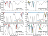 |
Fig. C.1 Same as Fig. 5 but for CH3CHO, CH3OCH3, and CH3COCH3. |
| In the text | |
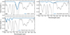 |
Fig. C.2 Same as Fig. 4 but for OCN−, CH3COOH, and CH3CN. |
| In the text | |
|
Fig. D.1 Baseline correction to lab spectra of ice mixtures. In the left panels, we take the H2O-rich mixtures of CH4 and three O-COMs (CH3CHO, C2H5OH, CH3OCH3) as examples. The original and the corrected spectra are plotted in solid blue and green, respectively. The polynomial is plotted in dashed orange, and the wavelength ranges that were selected to fit the polynomial are highlighted in orange panels. The right panels are similar to the left ones but for CH3OH mixtures. SO2, HCOOH, C2H5OH, and CH3OCH3 are taken as examples. The purple-shaded regions indicate the frequency ranges of CH3OH bands. |
| In the text | |
|
Fig. E.1 Best-fit LTE models overlaid on the observed ALMA spectrum of IRAS 2A. |
| In the text | |
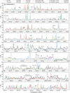 |
Fig. E.2 Same as Fig. E.1 but for B1-c. |
| In the text | |
|
Fig. F.1 Comparison between the lab spectra of pure H2CO ice (black), pure CH3OCHO ice (blue), and CH3OCHO:CO:H2CO:CH3OH mixture under 15 K (orange) and 80 K (dashed green). The corrected spectrum for the CH3OCHO mixture under 15 K (red) is plotted at an offset place. |
| In the text | |
|
Fig. F.2 Isolation of the CH3OCHO bands from the H2CO band in the lab spectrum of the CH3OCHO:CO:H2CO:CH3OH mixture. Top panel: H2CO band at 6.67 μm (blue) isolated by tracing a local continuum (orange) to the observed spectrum (black); superposed gas-phase absorption lines of H2O are not removed here. Bottom-left panel: lab spectra of pure H2CO ice (blue) and the CH3OCHO:CO:H2CO:CH3OH mixture (orange) manually scaled to the isolated H2CO band at 6.67 μm in observations (black). Bottom-right panel: same as the middle panel but for a different wavelength range (7.9–8.5 μm). |
| In the text | |
|
Fig. J.1 Fitting of the CH3OH bands at 3.94 and 9.74 μm. Top panel: the NIRSpec IFU spectrum of B1-c (solid black) and the local continuum of the 3.94μm CH3OH band fit by a 3rd-order polynomial (dashed red). Bottom-left panel: best-fit results of the observed absorption complex between 3.75 and 4.03 μm (black, the same as in the top panel but in optical depth scale). The shaded regions in red and yellow correspond to the CH3OH and H2S components, respectively. The overall best-fit spectrum is shown in dashed green. Bottom-right panel: the observed 9.74 μm band in the MIRI-MRS spectrum (black) overlaid with the CH3OH:H2O lab spectrum (red) scaling with the same factor as in the middle panel. |
| In the text | |
Current usage metrics show cumulative count of Article Views (full-text article views including HTML views, PDF and ePub downloads, according to the available data) and Abstracts Views on Vision4Press platform.
Data correspond to usage on the plateform after 2015. The current usage metrics is available 48-96 hours after online publication and is updated daily on week days.
Initial download of the metrics may take a while.